crack imaging by scanning pulsed laser spot...

NDT&E International ] (]]]]) ]]]–]]]

Contents lists available at ScienceDirect

NDT&E International

0963-86

doi:10.1

n Corr

E-m

Pleasj.ndt

journal homepage: www.elsevier.com/locate/ndteint

Crack imaging by scanning pulsed laser spot thermography

Teng Li, Darryl P. Almond n, D.Andrew S. Rees

UK Research Centre in NDE (RCNDE), Department of Mechanical Engineering, University of Bath, Claverton Down, Bath BA2 7AY, UK

a r t i c l e i n f o

Article history:

Received 9 December 2009

Received in revised form

18 August 2010

Accepted 19 August 2010

Keywords:

Infrared thermography

Laser

Thermal imaging

Simulation

Finite difference method

Cracks

Image processing

95/$ - see front matter & 2010 Elsevier Ltd. A

016/j.ndteint.2010.08.006

esponding author.

ail address: [email protected] (D.P. Alm

e cite this article as: Li T, et al. Craeint.2010.08.006

a b s t r a c t

A new crack imaging technique is presented that is based on second derivative image processing of

thermal images of laser heated spots. Experimental results are shown that compare well with those

obtained by the dye penetrant inspection method. A 3D simulation has been developed to simulate heat

flow from a laser heated spot in the proximity of a crack. A ‘ghost point’ method has been used to deal

efficiently with cracks having openings in the micometre range. Results are presented showing the

effects of crack geometry and system parameters on thermal images of laser heated spots.

& 2010 Elsevier Ltd. All rights reserved.

1. Introduction

Pulsed thermography (PT) is a non-contact, quick inspectionmethod that detects in-plane defects such as delaminations andimpact damage [1–4]. It is a technique that is not suitable for thedetection of important surface breaking cracks in metals causedby fatigue or creep. These cracks, which grow predominantlyperpendicular to the material surface, typically have openings of afew microns. It has been reported that surface cracks withopenings (widths) of below 0.5 mm on a concrete surface couldnot be detected by PT [5]. In the laser spot thermography (LST)technique, a laser provides a highly localized heating spot. Heatflow in the volume of the material from such a spot presents arelatively symmetrical half-spherical shape in the radial direc-tions if the material is thermally isotropic. Perpendicular cracks,close to the heated spot, will perturb the round lateral heat flowand the perturbation may be detected by a thermal camera toreveal the cracks. Preliminary studies [6–14] showed that theshape of the heat flow at certain times was deformed clearly byperpendicular cracks. Based on the previous studies, a full 3D‘ghost point’ heat transfer finite difference model has beendeveloped to predict the thermal behaviour of laser spot heatedmaterial in the proximity of a crack. Furthermore, a new imageprocessing technique has been developed to form a direct imageof a crack.

ll rights reserved.

ond).

ck imaging by scanning pu

2. ‘Ghost point’ heat diffusion model

Modelling has been used to gain an understanding of the optimumoperating parameters for the laser spot thermography technique andto assess the theoretical limits of its sensitivity for the detection ofcracks. The effects of cracks may be simulated by ‘ghost points’ in anumerical modelling grid that are generated by balancing thermalfluxes flowing into a crack and through a crack, with those flowingout of the crack according to Fourier’s law. They guarantee correctthermal gradients in the bulk material on either side of the crack.

The concept of the ‘ghost point’ in a 1D finite difference heattransfer model is shown in Fig. 1. In this case, the crack is embeddedbetween the current grid point ‘i’ and its left grid point ‘i�1’. Thewidth of the crack ‘d’ may be far smaller than the grid spacing ‘d’.The distance of the crack to the left grid point is ‘s’. Usually, thecrack is full of air and its conductivity ‘Ka’ is much lower than theconductivity of the metal block ‘Ks’. Thus thermal gradient across thecrack will be larger than in other parts of the metal block.

Heat flux balance in the x direction when it flows from the gridpoint ‘i�1’ into the crack, through the crack, and then flows out ofthe crack to the grid point ‘i’ gives

KsTL�Ti�1

s ¼ KaTR�TL

d¼ Ks

Ti�TR

d�s�d ¼ g ð1Þ

where Ti�1, TL, TR, Ti and Ti +1 are, respectively, the temperaturerise at the grid point ‘i�1’, the left boundary of the crack, the rightboundary of the crack and the grid points of ‘i’ and ‘i+1’; g is theheat flux.

Eq. (2) shows the calculation of temperature rise at the ‘ghostpoint’. By defining a ‘ghost point’ to equal the temperature

lsed laser spot thermography. NDT&E Int (2010), doi:10.1016/

www.elsevier.com/locate/ndteint

dx.doi.org/10.1016/j.ndteint.2010.08.006

mailto:[email protected]





TG

KaTi-1

Ks

TR

dx

Ghost point

TL

δσ

Ti

Ti+1

Fig. 1. 1D ‘ghost point’ finite difference heat diffusion model. Heat flux is balanced

when it flows into, through and out of the crack.

Table 1Parameters used in the simulations.

Material Thermal

conductivity

K (W/m K)

Specific heat

C (J/kg K)

Mass density

r (kg/m3)

Thermal

diffusivity

k¼K/rC (m/s2)

Air 0.025 1000 1.205 2.0747�10�5

Mild steel 40 500 7850 1.0191�10�5

Stainless steel 13.5 485 7900 3.5234�10�6

Fig. 2. Experimental setup.

T. Li et al. / NDT&E International ] (]]]]) ]]]–]]]2

increase effect because of the crack, the ‘isotropic’ heat transfermodel can still be applied; however, temperature rise at the gridpoint ‘i�1’ should be replaced by the value of the ‘ghost point’ TG:

KsTi�TG

d¼ g ð2Þ

After substituting Eq. (1) in Eq. (2), we can represent TG by Ti

and Ti�1:

TG ¼x

xþdTiþ

d

xþdTi�1 ð3Þ

where x is related with Ks, Ka and d:

x¼Ks

Ka�1

� �d ð4Þ

The 1D heat diffusion equation with no internal heat genera-tion is

k@2T

@x2¼@T

@tð5Þ

where k is the thermal diffusivity. Substituting Eq. (3) in Eq. (5),and representing Eq. (5) using finite difference elements, we canhave

Tmþ1i ¼

kDt

2dðTm

iþ1�aTmi þbTm

i�1ÞþTmi ð6Þ

where Dt is the time step, Tmi the temperature rise of the grid

point ‘i’ at time m and Tmþ1i the temperature rise at the next time

step. The values of a and b are

a¼xþ2d

xþdð7Þ

b¼d

xþdð8Þ

If the heat diffusion model is 2D, then the value of a becomes

a¼3xþ4d

xþdð9Þ

Similarly, in the 3D heat diffusion model, a has the value

a¼5xþ6d

xþdð10Þ

If the crack is embedded between current grid point i’ andpoint ‘i+1’, then grid point ‘i+1’ becomes the ‘ghost point’ andtemperature rise at this point should multiply the coefficient b

like the ghost point ‘i�1’ in Eq. (6).Furthermore, the temperature gradient across the crack can

also be derived from Eq. (1) as follows:

TR�TL

d¼

Ti�Ti�1

Ka=Ksðd�dÞþdð11Þ

Please cite this article as: Li T, et al. Crack imaging by scanning puj.ndteint.2010.08.006

By using the ‘ghost points’ to balance the heat flux, the heattransfer model avoids the need of very fine mesh spacing that isnecessary to deal with real cracks that often have openings of onlya few micrometres [6,7]. In the following simulations, theboundary conditions for all metal samples are assumed to beinsulated. Table 1 shows the property parameters used in thesimulations for the air gap and two types of steel.

3. Experimental and modelling results

3.1. Modelling validation

Previous publications using the 2D ghost point method [6,7]gave an indication of the way in which defect opening and hostmaterial affect LST response. In this research, a full 3D ghost pointmodel was developed to enable a comprehensive investigation ofall factors that affect the response of the technique. A furtherdifference is that a much higher power laser was used in thecurrent work. The previous work [6,7] was completed using laserpowers of o1 W, whilst in the current work a 21 W Laservallindustrial fibred diode welding/brazing laser has been used. Thelaser beam wavelength is 808 nm and its focal spot diameter isabout 1.8 mm. The laser is operated in a pulse mode. The pulsewidth can be set from 1 ms to 10 s.

Fig. 2 shows the experimental setup. A computer is used tocontrol the translation stage to move either the test-piece or thelaser head (Fig. 2 shows only one arrangement). The computeralso controls the laser output power and pulse duration. Theinfrared camera used to record the thermal images was a MerlinMID (Indigo Systems Cooperation) with a frame rate of 60 Hz.Thermal images are stored into a second computer for post-processing.

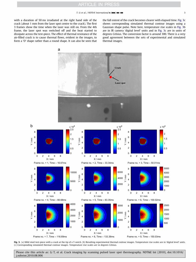
Fig. 3a shows a mild steel test-piece (painted with black paint onthe surface) with a fatigue crack developed vertically at the tip of aT-notch. The crack opening (width) is about 50 mm, length is about5 mm and depth is about 4 mm. Fig. 3b shows the resulting thermalcontour images obtained after subtracting the background thermalimage. The first 9 frames are shown after a 13 W laser spot heating




T. Li et al. / NDT&E International ] (]]]]) ]]]–]]] 3

with a duration of 50 ms irradiated at the right hand side of thecrack (about 1 mm from the laser spot centre to the crack). The first3 frames show the time when the laser was still on. From the 4thframe, the laser spot was switched off and the heat started todissipate across the test-piece. The effect of thermal resistance of theair-filled crack is to cause thermal flows, evident in the images, toform a ‘D’ shape rather than a round shape. It can also be seen that

X / mm X / mm

X / mm X / mm

X / mm X / mm

Frame no. = 1, Time ≈ 16.67ms

Y /

mm

Y /

mm

Y /

mm

Y /

mm

Y /

mm

Y /

mm

0 2 4 6 80

2

4

6

8

0

0.5

1

1.5

2

2.5x 104

Frame no. = 2, Time

0 2 4 60

2

4

6

8


0 2 4 6 80

2

4

6

8

0

5000

10000

Frame no. = 5, Time

0 2 4 60

2

4

6

8


0 2 4 6 80

2

4

6

8

0

1000

2000

3000

4000

Frame no. = 8, Time

0 2 4 60

2

4

6

8

Fig. 3. (a) Mild steel test-piece with a crack at the tip of a T-notch. (b) Resulting experi

(c) Corresponding simulated thermal contour images. Temperature rise scales are in d


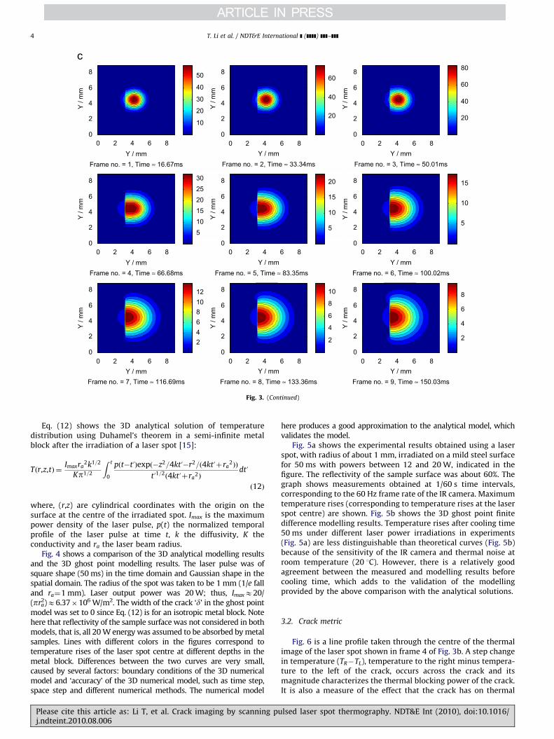
the full extent of the crack becomes clearer with elapsed time. Fig. 3cshows corresponding simulated thermal contour images using aGaussian shape pulse. Note here, temperature rise scales in Fig. 3bare in IR camera ‘digital level’ units and in Fig. 3c are in units ofdegrees Celsius. The conversion factor is around 300. There is a verygood agreement between the sets of experimental and simulatedthermal images.

Crack

Laser spot

X / mm

X / mm

X / mm

Y /

mm

Y /

mm

Y /

mm

x 104 x 104

≈ 33.34ms

8

0.5

1

1.5

2

2.5


0 2 4 6 80

2

4

6

8

0.5

1

1.5

2

≈ 83.35ms

80

2000

4000

6000


0 2 4 6 80

2

4

6

8

0

1000

2000

3000

4000

5000

≈ 133.36ms

80

1000

2000

3000


0 2 4 6 80

2

4

6

8

500

1000

1500

2000

2500

mental thermal contour images. Temperature rise scales are in ‘digital level’ units.

egrees Celsius.





Y /

mm

Y / mm Y / mm Y / mm



Y /

mm

Y /

mm

Y /

mm

Y /

mm

Y /

mm

Y /

mm

Y /

mm

Y /

mm

0 2 4 6 80

2

4

6

8


0 2 4 6 80

2

4

6

8


0 2 4 6 80

2

4

6

8


0 2 4 6 80

2

4

6

8


0 2 4 6 80

2

4

6

8


0 2 4 6 80

2

4

6

8


0 2 4 6 80

2

4

6

8


0 2 4 6 80

2

4

6

8


0 2 4 6 80

2

4

6

8

10

20

30

40

50

20

40

60

20

40

60

80

51015202530

5

10

15

20

5

10

15

24681012

2

4

6

8

10

2

4

6

8

Fig. 3. (Continued)


Eq. (12) shows the 3D analytical solution of temperaturedistribution using Duhamel’s theorem in a semi-infinite metalblock after the irradiation of a laser spot [15]:

Tðr,z,tÞ ¼Imaxra

2k1=2

Kp1=2

Z t

0

pðt�tuÞexpð�z2=4ktu�r2=ð4ktuþra2ÞÞ

tu1=2ð4ktuþra

2Þdtu

ð12Þ

where, (r,z) are cylindrical coordinates with the origin on thesurface at the centre of the irradiated spot. Imax is the maximumpower density of the laser pulse, p(t) the normalized temporalprofile of the laser pulse at time t, k the diffusivity, K theconductivity and ra the laser beam radius.

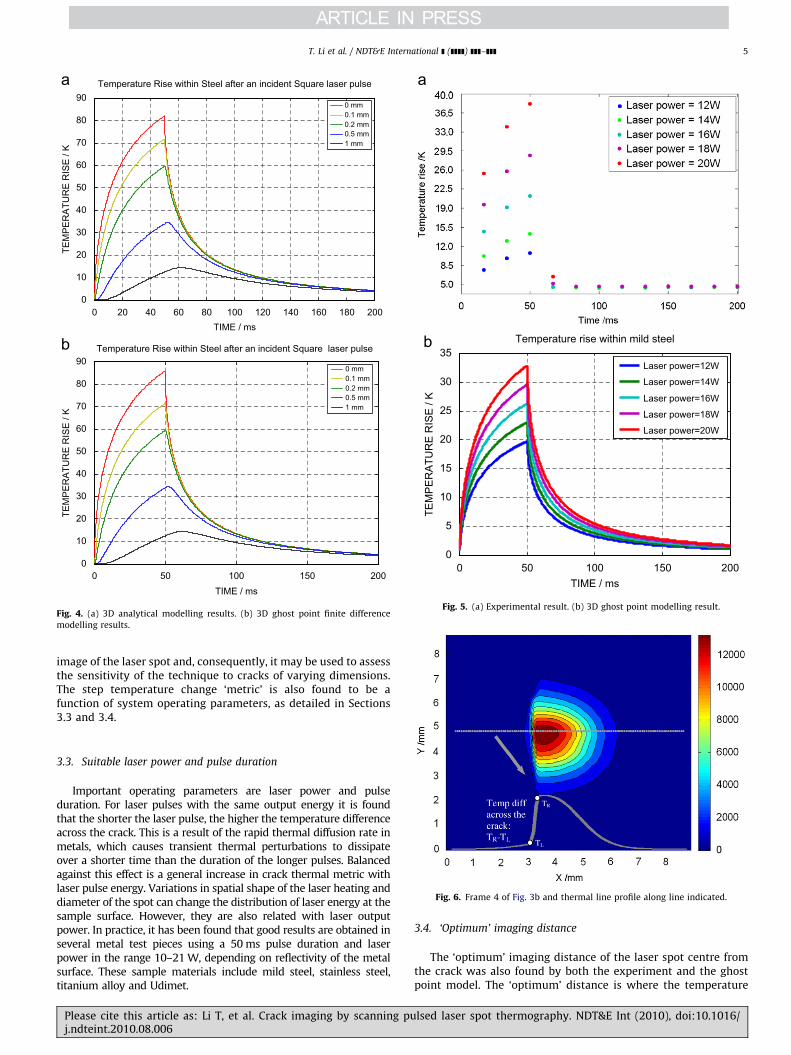
Fig. 4 shows a comparison of the 3D analytical modelling resultsand the 3D ghost point modelling results. The laser pulse was ofsquare shape (50 ms) in the time domain and Gaussian shape in thespatial domain. The radius of the spot was taken to be 1 mm (1/e falland ra¼1 mm). Laser output power was 20 W; thus, ImaxE20/(pra

2)E6.37�106 W/m2. The width of the crack ‘d’ in the ghost pointmodel was set to 0 since Eq. (12) is for an isotropic metal block. Notehere that reflectivity of the sample surface was not considered in bothmodels, that is, all 20 W energy was assumed to be absorbed by metalsamples. Lines with different colors in the figures correspond totemperature rises of the laser spot centre at different depths in themetal block. Differences between the two curves are very small,caused by several factors: boundary conditions of the 3D numericalmodel and ‘accuracy’ of the 3D numerical model, such as time step,space step and different numerical methods. The numerical model


here produces a good approximation to the analytical model, whichvalidates the model.

Fig. 5a shows the experimental results obtained using a laserspot, with radius of about 1 mm, irradiated on a mild steel surfacefor 50 ms with powers between 12 and 20 W, indicated in thefigure. The reflectivity of the sample surface was about 60%. Thegraph shows measurements obtained at 1/60 s time intervals,corresponding to the 60 Hz frame rate of the IR camera. Maximumtemperature rises (corresponding to temperature rises at the laserspot centre) are shown. Fig. 5b shows the 3D ghost point finitedifference modelling results. Temperature rises after cooling time50 ms under different laser power irradiations in experiments(Fig. 5a) are less distinguishable than theoretical curves (Fig. 5b)because of the sensitivity of the IR camera and thermal noise atroom temperature (20 1C). However, there is a relatively goodagreement between the measured and modelling results beforecooling time, which adds to the validation of the modellingprovided by the above comparison with the analytical solutions.

3.2. Crack metric

Fig. 6 is a line profile taken through the centre of the thermalimage of the laser spot shown in frame 4 of Fig. 3b. A step changein temperature (TR�TL), temperature to the right minus tempera-ture to the left of the crack, occurs across the crack and itsmagnitude characterizes the thermal blocking power of the crack.It is also a measure of the effect that the crack has on thermal




0 20 40 60 80 100 120 140 160 180 2000

10

20

30

40

50

60

70

80

90

TIME / ms

TEM

PE

RA

TUR

E R

ISE

/ K

Temperature Rise within Steel after an incident Square laser pulse

0 mm0.1 mm0.2 mm0.5 mm1 mm

0 50 100 150 2000

10

20

30

40

50

60

70

80

90

TIME / ms

TEM

PE

RA

TUR

E R

ISE

/ K

Temperature Rise within Steel after an incident Square laser pulse

0 mm0.1 mm0.2 mm0.5 mm1 mm

Fig. 4. (a) 3D analytical modelling results. (b) 3D ghost point finite difference

modelling results.

0 50 100 150 2000

5

10

15

20

25

30

35

TIME / ms

TEM

PE

RA

TUR

E R

ISE

/ K

Temperature rise within mild steel

Laser power=12W

Laser power=14W

Laser power=16W

Laser power=18W

Laser power=20W

Fig. 5. (a) Experimental result. (b) 3D ghost point modelling result.


image of the laser spot and, consequently, it may be used to assessthe sensitivity of the technique to cracks of varying dimensions.The step temperature change ‘metric’ is also found to be afunction of system operating parameters, as detailed in Sections3.3 and 3.4.

Fig. 6. Frame 4 of Fig. 3b and thermal line profile along line indicated.

3.3. Suitable laser power and pulse duration

Important operating parameters are laser power and pulseduration. For laser pulses with the same output energy it is foundthat the shorter the laser pulse, the higher the temperature differenceacross the crack. This is a result of the rapid thermal diffusion rate inmetals, which causes transient thermal perturbations to dissipateover a shorter time than the duration of the longer pulses. Balancedagainst this effect is a general increase in crack thermal metric withlaser pulse energy. Variations in spatial shape of the laser heating anddiameter of the spot can change the distribution of laser energy at thesample surface. However, they are also related with laser outputpower. In practice, it has been found that good results are obtained inseveral metal test pieces using a 50 ms pulse duration and laserpower in the range 10–21 W, depending on reflectivity of the metalsurface. These sample materials include mild steel, stainless steel,titanium alloy and Udimet.


3.4. ‘Optimum’ imaging distance

The ‘optimum’ imaging distance of the laser spot centre fromthe crack was also found by both the experiment and the ghostpoint model. The ‘optimum’ distance is where the temperature




-4 -2 0 2 40

5

10

15

20

25

30

Tem

p. d

iff. a

cros

s th

e cr

ack

/ K

Distance of laser to crack / mm

-0.9mm

Fig. 7. Temperature differences across the crack when the spot centre has

different distances to the crack: (a) experimental results, expressed in IR camera

digital levels and (b) modelling results.

0 2 4 6 8 100

5

10

15

20

Crack length / mm

Tem

p. d

iff. a

cros

s th

e cr

ack

/ K Crack depth: 2mm; crack opening: 10 μmLaser to crack: -1mm; laser radius: 0.9mm

0 1 2 3 4 50

5

10

15

20

25

Crack depth / mm

Tem

p. d

iff. a

cros

s th

e cr

ack

/ K

Crack depth: 2mm; crack opening: 10 μmLaser to crack: -1mm; laser radius: 0.9mm

0 20 40 60 80 1000

5

10

15

20

25

30

Tem

p. d

iff. a

cros

s th

e cr

ack

/ K

Crack opening / μm

Crack depth: 2mm; crack depth: 2mmLaser to crack: -1mm; laser radius: 0.9mm

5 μm

Fig. 8. Dependence of temperature differences across the crack on (a) crack

opening, (b) crack length and (c) crack depth.


difference across the crack has the largest value. Thus the thermalgradient across the crack reaches the largest value too. Fig. 7ashows the maximum temperature difference (near the laser spotcentre) across the crack when the spot centre has differentdistances to the crack (moving along a line through the spotcentre perpendicular to the crack). The same test-piece shown inFig. 3a was used in the experiment. The laser radius was about1.25 mm. It is shown in Fig. 7a that the maximum temperaturedifference across the crack occurs at the position when the laserspot centre is 1 beam radius (1/e fall) away from the crack. Fig. 7bshows the modelling result by using the 3D ghost point model.The laser radius was 0.9 mm (1/e fall). Simulated crack openingwas 10 mm, length was 2 mm and depth was 2 mm. Temperaturedifference across the crack reaches the maximum value when thedistance of the laser spot centre to the crack was 0.9 mm. Thereflectivity of the sample surface was set at 50%. Again, themodelling result shows that the ‘optimum’ imaging distance isone radius of the spot.

3.5. Variations in crack parameters

Fig. 8a shows modelling results of variations in temperaturedifference across a crack with different openings in a mild steelblock (10 mm�10 mm�5 mm). The laser spot radius was


0.9 mm and the spot was centred at the position near theoptimum position, one beam radius from the crack. The laseroutput power and pulse duration were assumed, respectively, to




-6

-4

-2 20

25


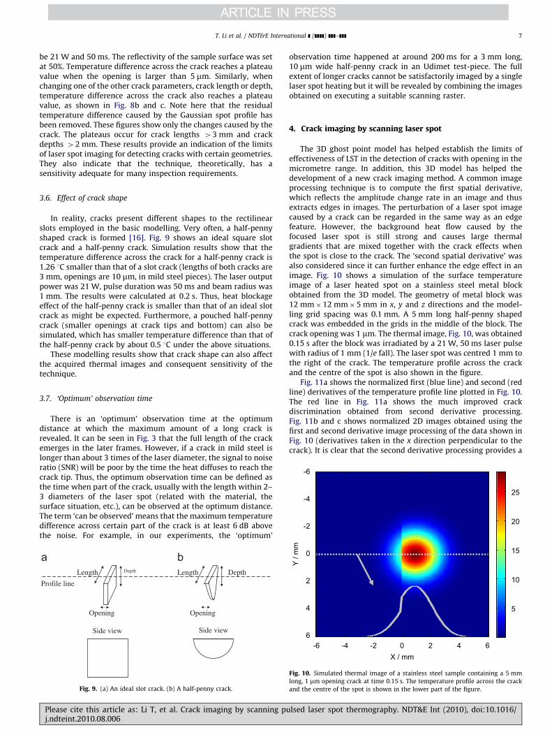
be 21 W and 50 ms. The reflectivity of the sample surface was setat 50%. Temperature difference across the crack reaches a plateauvalue when the opening is larger than 5 mm. Similarly, whenchanging one of the other crack parameters, crack length or depth,temperature difference across the crack also reaches a plateauvalue, as shown in Fig. 8b and c. Note here that the residualtemperature difference caused by the Gaussian spot profile hasbeen removed. These figures show only the changes caused by thecrack. The plateaus occur for crack lengths 43 mm and crackdepths 42 mm. These results provide an indication of the limitsof laser spot imaging for detecting cracks with certain geometries.They also indicate that the technique, theoretically, has asensitivity adequate for many inspection requirements.

3.6. Effect of crack shape

In reality, cracks present different shapes to the rectilinearslots employed in the basic modelling. Very often, a half-pennyshaped crack is formed [16]. Fig. 9 shows an ideal square slotcrack and a half-penny crack. Simulation results show that thetemperature difference across the crack for a half-penny crack is1.26 1C smaller than that of a slot crack (lengths of both cracks are3 mm, openings are 10 mm, in mild steel pieces). The laser outputpower was 21 W, pulse duration was 50 ms and beam radius was1 mm. The results were calculated at 0.2 s. Thus, heat blockageeffect of the half-penny crack is smaller than that of an ideal slotcrack as might be expected. Furthermore, a pouched half-pennycrack (smaller openings at crack tips and bottom) can also besimulated, which has smaller temperature difference than that ofthe half-penny crack by about 0.5 1C under the above situations.

These modelling results show that crack shape can also affectthe acquired thermal images and consequent sensitivity of thetechnique.

3.7. ‘Optimum’ observation time

There is an ‘optimum’ observation time at the optimumdistance at which the maximum amount of a long crack isrevealed. It can be seen in Fig. 3 that the full length of the crackemerges in the later frames. However, if a crack in mild steel islonger than about 3 times of the laser diameter, the signal to noiseratio (SNR) will be poor by the time the heat diffuses to reach thecrack tip. Thus, the optimum observation time can be defined asthe time when part of the crack, usually with the length within 2–3 diameters of the laser spot (related with the material, thesurface situation, etc.), can be observed at the optimum distance.The term ‘can be observed’ means that the maximum temperaturedifference across certain part of the crack is at least 6 dB abovethe noise. For example, in our experiments, the ‘optimum’

Depth

Side view Side view

Opening

Length

Opening

Length Depth

Profile line

Fig. 9. (a) An ideal slot crack. (b) A half-penny crack.


observation time happened at around 200 ms for a 3 mm long,10 mm wide half-penny crack in an Udimet test-piece. The fullextent of longer cracks cannot be satisfactorily imaged by a singlelaser spot heating but it will be revealed by combining the imagesobtained on executing a suitable scanning raster.

4. Crack imaging by scanning laser spot

The 3D ghost point model has helped establish the limits ofeffectiveness of LST in the detection of cracks with opening in themicrometre range. In addition, this 3D model has helped thedevelopment of a new crack imaging method. A common imageprocessing technique is to compute the first spatial derivative,which reflects the amplitude change rate in an image and thusextracts edges in images. The perturbation of a laser spot imagecaused by a crack can be regarded in the same way as an edgefeature. However, the background heat flow caused by thefocused laser spot is still strong and causes large thermalgradients that are mixed together with the crack effects whenthe spot is close to the crack. The ‘second spatial derivative’ wasalso considered since it can further enhance the edge effect in animage. Fig. 10 shows a simulation of the surface temperatureimage of a laser heated spot on a stainless steel metal blockobtained from the 3D model. The geometry of metal block was12 mm�12 mm�5 mm in x, y and z directions and the model-ling grid spacing was 0.1 mm. A 5 mm long half-penny shapedcrack was embedded in the grids in the middle of the block. Thecrack opening was 1 mm. The thermal image, Fig. 10, was obtained0.15 s after the block was irradiated by a 21 W, 50 ms laser pulsewith radius of 1 mm (1/e fall). The laser spot was centred 1 mm tothe right of the crack. The temperature profile across the crackand the centre of the spot is also shown in the figure.

Fig. 11a shows the normalized first (blue line) and second (redline) derivatives of the temperature profile line plotted in Fig. 10.The red line in Fig. 11a shows the much improved crackdiscrimination obtained from second derivative processing.Fig. 11b and c shows normalized 2D images obtained using thefirst and second derivative image processing of the data shown inFig. 10 (derivatives taken in the x direction perpendicular to thecrack). It is clear that the second derivative processing provides a

X / mm

Y /

mm

-6 -4 -2 0 2 4 6

0

2

4

6

5

10

15

Fig. 10. Simulated thermal image of a stainless steel sample containing a 5 mm

long, 1 mm opening crack at time 0.15 s. The temperature profile across the crack

and the centre of the spot is shown in the lower part of the figure.




-6 -4 -2 0 2 4 6-1.5

-1

-0.5

0

0.5

1

X / mm

First derivativeSecond derivative

X / mmY

/ m

m-6 -4 -2 0 2 4 6

-6

-4

-2

0

2

4

6 0

0.2

0.4

0.6

0.8

1

X / mm

Y /

mm

-6 -4 -2 0 2 4 6

-6

-4

-2

0

2

4

6 0

0.2

0.4

0.6

0.8

1

Fig. 11. (a) Normalized first (blue line) and second (red line) derivatives of the temperature profile line in Fig. 10. (b). First derivative image in x direction of Fig. 10 image.

(b) Second derivative image in x direction of Fig. 10 image. (For interpretation of the references to colour in this figure legend, the reader is referred to the web version of

this article.)

X / mm

Y /

mm

-6 -4 -2 0 2 4 6

-6

-4

-2

0

2

4

6 0

0.2

0.4

0.6

0.8

1

X / mm

Y /

mm

-6 -4 -2 0 2 4 6

-6

-4

-2

0

2

4

6 0

0.2

0.4

0.6

0.8

1

Fig. 12. (a) Summed second derivative image in x direction from 0.05 to 0.3 s. (c) Summed second derivative image in x direction from 0.05 to 0.3 s.


better means of isolating the image of the crack. The contrast ofthe crack to the background heat flow (ratio of the maximumamplitude at crack positions to the maximum amplitude of thebackground heat flow) in Fig. 11b is about 3.21. In Fig. 11c, thecontrast becomes 9.79, which is 3.05 times higher than that inFig. 11b.

In practice, image acquisition time and noise need to beconsidered. The simulation shown in Fig. 10 corresponds to animage that might be collected by a thermal imaging camera, 0.15 safter the extinction of a laser heating pulse. In practice, morethermal images at different times can be used. This provides theopportunity to form a summed thermal image that will furtheremphasize the crack structure over the background heat flow.However, the second derivative method is known to be sensitive tonoise [17]; hence only thermal images with high signal to noise ratioshould be considered. The effects of image addition and noise wereinvestigated by adding 70.15 K (one standard deviation) randomnoise to the above model and summing first and then secondderivative thermal images from 0.05 s after the extinction of a laserheating pulse to 0.3 s, when the remaining heating becamecomparable to the noise level. Images were computed at intervalsof 1/60 s matching the 60 Hz frame rate of the IR camera used in theexperimental work below. The normalized first and secondderivative images are shown in Fig. 12a and b, respectively. Afterintegrating thermal images at different times, the contrast of thecrack to the background heat flow in Fig. 12a is 7.23. In Fig. 12b, the


contrast is 27.76, which is 3.8 times higher than that in Fig. 12a. Inaddition, the integration method improves the contrast by 2.8 timesin Fig. 12b compared to Fig. 11c.

The crack length indicated by the single spot images shown inFig. 10 is about 3.8 mm, which is somewhat shorter than the true5 mm crack length. In practice the location of a crack might beunknown and a raster scanning technique would be used. Acombination of results obtained from such scans will improve thesizing of cracks, as shown in the experimental work below.

A test-piece containing a crack was raster scanned using 21 W,50 ms laser heating pulses. The laser spot radius was 1 mm (1/efall) and the IR camera field of view was 26.4�20.8 mm2. Theprocessing steps performed on the thermal images from the IRcamera are as follows:

1.

lse

Subtract the background IR image to produce a dark-fieldimage showing only the transient heat diffusion (this can beeasily done by subtracting a thermal image obtained before thelaser was switched on), and then compute the secondderivative of each dark-field image at each scanning step inboth x and y directions. Note here, the dark-field image at eachposition can be the averaged image of several pre-imagestaken by the camera before the laser spot is switched onat each position on the specimen surface or any one of thepre-images.

d laser spot thermography. NDT&E Int (2010), doi:10.1016/




2.

Fig3.44

Figima

Pj.

Integrate all second derivative images in x or y directioncollected from 0.05 to 0.3 s at each scanning position.

3.

Fig. 15. Summed second derivative image of an 8 mm long crack with opening

less than 1 mm.

Form a composite image of all the integrated images obtainedat the different scanning positions. A final sum image can beobtained by adding the squares of the two second derivativeimages in x and y directions to show the derivative informationin both x and y directions at the same time.

Fig. 13a shows a dye penetrant inspection ( DPI) image of an11 mm long, 3 mm deep crack with average opening of 24.5 mm ina test-piece (austenitic stainless steel) [18]. The images shown inFig. 13b and c were obtained using the above image processingmethods after scanning the test-piece. Fig. 13b shows the secondderivative image in x and Fig. 13c in the y direction. Since thecrack was orientated at an angle of approximately 451, signalamplitudes for the crack in Fig. 13b and c are similar. These crackimages are in good agreement with the DPI image of the crackshown in Fig. 13a. Information about crack shape and distributionof crack opening can also be seen in the image; it shows strongersignals in the middle part of the crack, where the crack is mostopen.

Raster scanning steps of 0.43 mm in the x direction and0.5 mm in the y direction were used to obtain the images shownin Fig. 13. Investigations were made on the images produced bycoarser scanning rasters. The images obtained after increasingscanning steps to 2.58 and 3.44 mm in the x direction are shownin Fig. 14. Most parts of the crack can still be seen using these

X / mm

Y /

mm

0 5 10 15 20 25

0

5

10

15

20

. 14. (a) Summed second derivative image in x direction with scanning step of 2.5

mm.

X / mm

Y /

mm

0 5 10 15 20

0

5

10

15

20

. 13. (a) Dye penetrant image of the crack in the test-piece. (b) Summed second x

ge of the crack. Scanning steps 0.43 and 0.5 mm in x and y directions, respectively

lease cite this article as: Li T, et al. Crack imaging by scanning pundteint.2010.08.006

coarser scanning rasters. This indicates that the crack imagingprocess may be speeded up by using coarser scanning rasters butit should be recognized that size of the minimum detectable crackwill be an increasing function of raster step length.

An image of a smaller, �8 mm long crack in an Udimet test-piece with an opening of less than 1 mm is shown in Fig. 15. Thisprovides evidence of the remarkable sensitivity of the technique.

X / mm

Y /

mm

0 5 10 15 20 25

0

5

10

15

20

8 mm. (b) Summed second derivative image in x direction with scanning step of

25X / mm

Y /

mm

0 5 10 15 20 25

0

5

10

15

20

direction derivative image of the crack. (c) Summed second y direction derivative

.





5. Discussion and conclusions

The modelling results presented in this paper indicate the laserspot thermography technique to have a sensitivity to cracks thatis competitive with most established NDE techniques. Thetechnique has the advantages of being non-contactive andrequiring no surface preparation. However, it is known that forthe technique to be successful, surfaces should be clean and freeof deep scratches or indentations that would perturb heat flow ina similar manner to a crack. To date, studies have been made onlyon surface breaking cracks. The ability of the technique to detectcracks beneath coatings is under investigation.

This paper also presents a novel second derivative imageprocessing method for extracting images of cracks after rasterscanning. The results obtained show scanned pulse laser spotthermography, incorporating second derivative image processing,to be a new effective nondestructive evaluation technique fordetecting and imaging surface breaking cracks with openings inthe range of micrometres. Crack images obtained by the newtechnique are at least comparable to those obtained by the longestablished DPI method. In addition, this new technique has theadvantages of eliminating the long preparation time of the dyepenetrant technique, eliminating the use of undesirable liquids,being deployable remotely and being suitable for automation. Thepractical sensitivity and reliability of the technique are underinvestigation.

Acknowledgements

This research was funded as a targeted research project of theEngineering and Physical Science Research Council (EPSRC), UKResearch Centre in NDE (RCNDE). The work also received supportfrom Rolls Royce plc, RWE Npower and the National NuclearLaboratory. The authors are grateful to Ben Weekes of ourlaboratory at the University of Bath for the image shown in Fig. 15.


References

[1] Reynolds WN. Thermographic methods applied to industrial materials. Can JPhys 1986;64:1150–4.

[2] Milne JM, Reynolds WN. The non-destructive evaluation of composites and othermaterials by thermal pulse video thermography. Proc SPIE 1984;520:119–22.

[3] Lau SK, Almond DP, Milne JM. A quantitative analysis of pulsed videothermography. NDT&E Int 1991;24:195–202.

[4] Shepard SM, Lhota JR, Ahmed T. Flash thermography contrast model based onIR camera noise characteristics. Nondestr Test Eval 2007;22:113–26.

[5] Sham FC, Chen N, Hong L. Surface crack detection by flash thermography onconcrete surface. Insight 2008;50(5):240–3.

[6] Rashed A, Almond DP, Rees DAS, Burrows SE, Dixon S. Crack detection by laserspot imaging thermography. Rev Prog QNDE 2006;26:500–6.

[7] Burrows SE, Rashed A, Almond DP, Dixon S. Combined laser spot imagingthermography and ultrasonic measurements for crack detection. NondestrTest Eval 2007;22:217–27.

[8] Bantel T, Bowman D, Halase J, Kenue S, Krisher R, Sippel T. Automatedinfrared inspection of jet engine turbine blades. Proc SPIE 1985;581:18–23.

[9] Devitt J.W., Bantel T.E., Sparks J.M., Kania J.S. Apparatus and method fordetecting fatigue cracks using infrared thermography. US Patent 5111048, 1992.

[10] Gruss C, Balageas D. Theoretical and experimental applications of the flyingspot camera. In: . 1992; Proceedings of the 27th Eurotherm seminar onquantitative infrared thermography, QIRT. p. 19–24.

[11] Hermosilla-Lara S, Joubert PY, Placko D, Lepoutre F, PiriouM. Enhancement ofopen-cracks detection using a principal component analysis/wavelet techni-que in photothermal nondestructive testing. In: Proceedings of thequantitative infrared thermography seminar, QIRT, 2002. p. 41–6 [ArchivesQIRT 2002-002].

[12] Hermosilla-Lara S, Joubert PY, Placko D. Identification of physical effects inflying spot photothermal non-destructive testing. Eur Phys J Appl Phys2003;24:223–9.

[13] Krapez JC, Gruss C, Huttner R, Lepoutre F, Legrandjacques L. La cameraphotothermique—partie I: principe, modelisation, application a la detectionde fissures. Instrum Mes Metrol 2001;1:9–39. [in French].

[14] Krapez JC, Lepoutre F, Huttner R, Gruss C, Legrandjacques L, Piriou M, et al.La camera photothermique—partie II: applications industrielles, perspectivesdamelioration par un nouveau traitement dimage. Instrum Mes Metrol2001;1:41–67. [in French].

[15] Doyle PA. On epicentral waveforms for laser-generated ultrasound. J Phys D1986;19(9):1613–23.

[16] Tang Y, Yonezu A, Ogasawara N, Chiba N, Chen X. On radial crack and half-penny crack induced by Vickers indentation. Proc R Soc A 2008;464:2967–84.

[17] Gonzalez RC, Woods RE. Digital image processing. 3rd ed.. New Jersey:Prentice Hall; 2006. p. 702–5.

[18] Trueflaw Ltd., Espoo, Fl-02330, Finland.




crack imaging by scanning pulsed laser spot...

Documents