Seventh Edition

W. Phillips Shively University of Minnesota

P E A R S O N

Upper Saddle River, NJ 07458

Library of Congress Cataloging-in-Publication Data

Shively.W. Phillips, 1942-

The craft of political research / W. Phillips Shively. — 7th ed.

p. cm.

Includes bibliographical references and index.

ISBN-13: 978-0-13-602948-9 (alk. paper)

ISBN-10: 0-13-602948-5 (alk. paper)

1. Political science—Methodology. 2. Political science—Research. I. Title.

JA71.S45 2009

320.072—dc22

2007047170

Executive Editor: Dickson Musslewhite

Editor-in-Chief: Yolanda de Rooy

Associate Editor: Rob De George

Editorial Assistant: Synamin Ballatt

Senior Marketing Manager: Kate Mitchell

Marketing Assistant: Jennifer Lang

Managing Editor: Joanne Riker

Manufacturing Buyer: Wanda Rockwell

Creative Director: Christy Mahon

Cover Design Director: Jayne Conte

Cover Design: Jon Boylan

Cover Illustration/Photo: Getty Images, Inc.

Composition: Integra

Full-Service Project Management: Integra

Printer/Binder: Courier-Stoughton

Credits and acknowledgments borrowed from other sources and reproduced, with permission, in this

textbook appear on appropriate page within text.

Copyright © 2009, 2005, 2002 ,1998 ,1990 ,1980 by Pearson Education, Inc., Upper Saddle River,

New Jersey, 07458. All rights reserved. Printed in the United States of America. This publication is

protected by Copyright and permission should be obtained from the publisher prior to any prohibited

reproduction, storage in a retrieval system or transmission in any form or by any means, electronic,

mechanical, photocopying, recording, or likewise. For information regarding permission(s), write to:

Rights and Permissions Department.

Pearson Prentice Hall™ is a trademark of Pearson Education, Inc.

Pearson® is a registered trademark of Pearson pic

Prentice Hall® is a registered trademark of Pearson Education, Inc.

Pearson Education Ltd.

Pearson Education Singapore, Pte. Ltd.

Pearson Education, Canada, Ltd.

Pearson Education-Japan

Pearson Education Australia PTY, Ltd.

Pearson Education North Asia Ltd.

Pearson Educacion de Mexico, S.A. de C.V.

Pearson Education Malaysia, Pte. Ltd.

1 0 9 8 7 6 5 4 3 2 1

I S B N - 1 3 : c l 7 f l - D - 1 3 - b D 5 T 4 f l - c 1 I S B N - I D : D - i g - b D S T M f l - S

To BARBARA

L

Preface xi

Doing Research 1

Socia l R e s e a r c h 2

Types of Political Research 4

Research Mix 8

Evaluating Different Types of Research 10

E t h i c s of Pol i t ical Research 11

Political Theories and Research Topics

Causal i ty and Pol i t ical Theory 14

What D o e s G o o d Theory L o o k L i k e ? 15

Example of Elegant Research: Philip Converse

To Quantify or Not 20

C h o i c e of a Topic 22

Engineering Research 22

Theory-Oriented Research 23

Development of a Research D e s i g n 23

Observations, Puzzles, and the Construction of Theories 25

Contents Contents ix

A F e w B a s i c s of R e s e a r c h Des ign 78

Designs Without a Control Group 79

Use of a Control Group 82

True Experiment 83

Designs for Pol i t ical Research 84

Special Design Problem for Policy Analysis: Regression to the Mean 88

U s e of Varied Des igns and Measures 90

Example of Varied Designs and Measures 92

C o n c l u s i o n 93

Holding a Variable Constant 94

Further D i s c u s s i o n 96

7 Selection of Observations for Study 97

Sampl ing f rom a Population of Potential Observat ions 99

Random Sampling 99

Quasi-random Sampling 101

Purposive Sampling 102

Selection of Cases for Case Studies 103

Censored Data 103

When Scholars Pick the Cases They 're Interested In 104

When Nature Censors Data 106

Select ion A l o n g the Dependent Variable:

Don ' t Do It! 106

Select ion of C a s e s for C a s e Studies (Aga in ) 108

Another Strategy, However: S i n g l e - C a s e Studies Selected

for the Relat ionship Between the Independent

and Dependent Variables 109

Further D i s c u s s i o n 110

8 Introduction to Statistics: Measuring Relationships for Interval Data 111

Statistics 112

Importance of L e v e l s of Measurement 112

Work ing with Interval Da ta 113

Machiave l l ian Gu ide to Developing R e s e a r c h

Topics 28

Further D i s c u s s i o n 31

Importance of Dimensional Thinking 32

E n g l i s h as a Language for Research 33

Ordinary Language 34

Proper U s e of Mul t id imensional Words 37

Example of Dimensional Analysis 38

Further D i s c u s s i o n 40

Problems of Measurement: Accuracy 41

Rel iabi l i ty 45

Reliability as a Characteristic of Concepts 46

Testing the Reliability of a Measure 47

Validity 48

Some Examples 49

Checks for Validity 51

Impact of R a n d o m and Nonrandom Er rors 53

Importance of A c c u r a c y 54

Further D i s c u s s i o n 56

Problems of Measurement: Precision 57

Precis ion in Measures 58

Prec is ion in Measurement 62

Innate Nature of Levels of Measurement 63

The Sin of Wasting Information 64

Enrichment of the Level of Precision in Measurement

Examples of Enrichment 67

Quantifiers and Nonquantifiers Again 72

Further D i s c u s s i o n 73

Causal Thinking and Design of Research 74

Causal i ty : An Interpretation 75

E l iminat ion of Alternative C a u s a l Interpretations 76

Summary 77

Contents

I wrote this little book in 1970, when I was an assistant professor at Y a l e University.

In teaching a number of sections of Introduction to R e s e a r c h to undergraduates

there, I had found that the students benefited f rom an introduction that emphasized

the internal logic of research methods and the col lect ive, cooperative nature of the

research process. I cou ld not f ind a book that presented things in this way at a suffi­

ciently elementary level to be readi ly accessib le by undergraduates. A n d so I wrote

this book.

It has fo l lowed me through the rest of my career so far, and has given me

enormous pleasure. It has a lways seemed to me that it f i l ls a needed niche, and it has

been a thrill w h e n students have told me that they have benefited from it. I am

pleased that it still seems to be work ing for them.

W h i l e the general principles of good argument and investigation don't change,

I have made a number of additions and deletions over the last couple of editions to

reflect new possibi l i t ies in technique. In this seventh edition, I have updated a num­

ber of examples, I have improved on my treatment of the use of nominal variables in

regression analys is , and I have added a new discussion of the problem of comparing

units in regression analys is . I have also changed signif icantly the position I take on

the question of selecting cases for analysis .

I must also admit to a recent change of heart (or, perhaps, a return to old love).

Regular users of this text may recal l that a couple of editions ago, under prodding

from reviewers, I changed my example of elegant research f rom Phi l ip Converse 's

" O f T i m e and Partisan Stabil i ty" to Robert Putnam's Making Democracy Work.

Putnam's book and the resultant research program on socia l capital are of course

splendid, but I a lways regretted sacr i f ic ing Converse 's article. It is stil l the most

x i

Regression Analysis 113

Correlation Analysis 122

Correlation and Regression Compared 127

Problem of Measurement Error 130

Further D i s c u s s i o n 131

Introduction to Statistics: Further Topics on Measurement of Relationships 132

Measures of Relat ionship for Ord ina l Da ta 132

Measures of Relat ionship for Nomina l Data 136

Dichotomies and Regression Analysis 136

Log i t and Probit A n a l y s i s 139

Multivariate A n a l y s i s 141

C o n c l u s i o n 146

Introduction to Statistics: Inference, or How to Gamble on Your Research 148

L o g i c of Measur ing Signi f icance 149

E x a m p l e of Statistical Inference 150

Hypothesis Test ing 151

Null Hypothesis 152

Example: %2 153

Sampling Distribution 155

Importance of'N 158

Problem of Independent Observations 161

Signi f icance Test: A l w a y s N e c e s s a r y ? 162

Pol l ing and Signi f icance Tests 163

U s e s and Limitat ions of Statistical Tests 163

C o n c l u s i o n 164

Further D i s c u s s i o n 164

Where Do Theories Come From? 166

Selected Bibliography 170

Index 174

xi i Preface

beautiful piece of pol i t ical sc ience research I know. A n d so I returned in the sixth

ed i t ion—and continue in this seventh edi t ion—to " O f T i m e and Partisan Stability,"

and include with it the same explication of Markov chains that I used in those earlier

editions.

As you can no doubt tell f rom the tone of this preface, this is a book for wh ich

I have great affection. I hope you wi l l enjoy it as much as I have enjoyed it.

A C K N O W L E D G M E N T S

T h a n k s to the fol lowing reviewers for their helpful suggestions and comments: Terri

Susan F ine , Universi ty of Centra l F lor ida ; Garrett G lasgow, Universi ty of Ca l i forn ia

at Santa Barbara; and Patrick James, Universi ty of Southern Cal i forn ia .

W. Phillips Shively

Chapter I

Scholar ly research is excit ing and is fun to do. S o m e students, caught in the grind of

daily and term assignments, may not see it this way. But for people who can carry on

research in a more relaxed way, for professors or for students w h o can involve them­

selves in a long-range project, research may be a source of fascination and great

satisfaction.

Francis's preoccupation with DNA quickly became full-time. The first afternoon follow­

ing the discovery that A - T and G - C base pairs had similar shapes, he went back to his

thesis measurements, but his effort was ineffectual. Constantly he would pop up from his

chair, worriedly look at the cardboard models, fiddle with other combinations, and then,

the period of momentary uncertainty over, look satisfied and tell me how important our

work was. I enjoyed Francis's words, even though they lacked the casual sense of under­

statement known to be the correct way to behave in Cambridge. (Watson, 1968, p. 198) 1

T h i s is the way James D. Watson describes his and Franc is C r i c k ' s search for

the structure of the D N A molecule. The Double Helix, h is account of their work,

gives a good picture of the excitement of research. It is more gripping than most

mystery novels.

Al though research can be excit ing in this way, the sad fact is that writ ing

papers for courses is too often something of a drag. F i rs t of a l l , course papers are tied

to all sorts of rewards and pun ishments—your future earnings, the approval of

others, and so on. A l l of the anxiety associated with these vulnerabil i t ies comes ,

indirectly, to lodge on the paper. Yet this is probably a lesser cause for frustration

in student research. After a l l , each of these anxieties may also be present for

'Reprinted with permission from Watson, James D. The Double Helix (New York: Atheneum,

1968).

1

2 Chapter 1

professional scholars. A more important reason for the student's lack of enthusiasm

is the simple fact that a paper is generally regarded, by both teacher and student, as a

practice run, going through the motions of scholarship. Usua l ly , not enough time is

a l lowed for the student to think long and seriously about the subject, especial ly with

other papers competing for attention. A n d even when adequate time is a l lowed, there

usual ly is a feeling on both sides that this is "just a student paper"—that it doesn't

real ly matter how good it i s , that a student w i l l learn from doing the thing wrong.

Students must have the chance to learn from their own mistakes, but this attitude

toward the research work cheats them of the pleasure and excitement that research

can bring, of the feel ing of creating something that no one ever saw before.

There is probably no w a y out of this d i lemma. In a book such as this, I cannot

give you the drama and excitement of original research. I can only give my own

testimony, as one for w h o m research is very excit ing. But I can introduce you to

some selected problems you should be aware of i f you want to do good research

yoursel f or to evaluate the work of others. I also hope to make you aware of what a

chal lenging game it can be, and of how important inventiveness, originality, and

boldness are to good research.

S O C I A L R E S E A R C H

Soc ia l research is an attempt by socia l scientists to develop and sharpen theories that

give us a handle on the universe. Real i ty unrefined by theory is too chaotic for us to

absorb. S o m e people vote and others do not; in some elections there are major shifts,

in others there are not; some bi l ls are passed by Congress , others are not; economic

development programs succeed in some countries, but fail in others; sometimes war

comes, sometimes it does not. To have any hope of controll ing what happens, we

must understand w h y these things happen. A n d to have any hope of understanding

w h y they happen, we must simpl i fy our perceptions of reality.

Soc ia l scientists carry out this simpli f icat ion by developing theories. A theory

takes a set of s imi lar things that happen—say , the development of party systems in

d e m o c r a c i e s — a n d finds a c o m m o n pattern among them that a l lows us to treat each

of these different occurrences as a repeated example of the same thing. Instead of

having to think about a large number of disparate happenings, we need only think of

a single pattern with some variations.

F o r example, in his book on polit ical parties, Maur ice Duverger was concerned

with the question of why some countries develop two-party systems and others

develop multiparty systems (1963, pp. 2 0 6 - 2 8 0 ) . T h e initial reality was chaotic;

scores of countries were involved, with varying numbers and types of parties present

at different times in their histories. Duverger devised the theory that (1) if social

confl icts overlap, and (2) if the electoral system of the country does not penalize

smal l parties, the country w i l l develop a multiparty system; otherwise, the country

w i l l develop a two-party system.

H i s idea was that where there is more than one sort of polit ical confl ict going

on simultaneously in a country, and where the groups of people involved in these

Doing Research 3

confl icts overlap, there w i l l be more than two distinct poli t ical positions in the coun­

try. F o r example, a confl ict between workers and the middle c lass might occur at the

same time as a confl ict between Cathol ics and non-Cathol ics . T h e n , if these groups

overlapped so that some of the Cathol ics were workers and some were middle c lass ,

whi le some of the non-Cathol ics were workers and some were middle c lass , there

would be four distinct polit ical positions in the country: the Catho l ic worker

position, the non-Cathol ic worker posit ion, the Cathol ic middle -c lass posit ion, and

the non-Cathol ic middle-c lass position. T h e appropriate number of parties would

then tend to r ise, with one party corresponding to each distinct posit ion.

However , Duverger thought that this tendency could be short-circuited if the

electoral system were set up in such a way as to penal ize smal l par t ies—by requiring

that a candidate have a majority, rather than a plurality, of votes in a district, for

instance. T h i s requirement would force some of the distinct groups to compromise

their positions and merge into larger parties that would have a better chance of

winning elections. S u c h a process of consolidation logical ly would culminate in a

two-party system. To summarize the theory: A country w i l l develop a two-party

system (1) if there are only two distinct poli t ical positions in the country, or (2) if

despite the presence of more than two distinct poli t ical posit ions, the electoral law

forces people of diverse positions to consolidate into two large polit ical parties so as

to gain an electoral advantage.

Having formulated this theory, Duverger no longer had to concern himself s imul­

taneously with a great number of idiosyncratic party systems. He needed to think only

about a single developmental process, of which t i l those party systems were examples.

Something is a lways lost when we simpli fy reality in this way. By restricting

his attention to the number of parties competing in the system, for example,

Duverger had to forget about many other potentially interesting things, such as

whether any one of the parties was revolutionary, or how many of the parties had any

chance of getting a majority of the votes.

Note, too, that Duverger restricted himsel f in more than just his choice of a

theme: He chose deliberately to play down exceptions to his theory, although these

exceptions might have provided interesting additional information. Suppose, for

instance, that a country for wh ich his theory had predicted a two-party system devel­

oped a multiparty system instead. W h y was this so? Duverger might have cast around

to find an explanation for the exception to his theory, and he could have then incorpo­

rated that explanation into the original theory to produce a larger theory. Instead, when

faced with exceptions such as these, he chose to accept them as accidents. It was

necessary for h im to do this in order to keep the theory simple and to the point.

Otherwise, it might have grown as complex as the reality that it sought to simplify.

As you can see, there are costs in setting up a theory. B e c a u s e the theory

simpli f ies reality for us, it also generally requires that we both narrow the range of

reality we look at and oversimpli fy even the portion of reality that falls within that

narrowed range. As theorists, we a lways have to strike a balance between the

simplici ty of a theory and the number of exceptions we are w i l l ing to tolerate. We do

not real ly have any choice. Without theories, we are faced with the unreadable chaos

of reality.

4 Chapter 1

Actual ly , what social scientists do in developing theories is not different f rom

what we normally do every day in perceiving, or interpreting, our environment. Socia l

scientists merely interpret reality in a more systematic and explicit way. Without

theories, students of society are trapped. They are reduced to merely observing

events, without comment. Imagine a phys ic is t—or a fruit p icker for that matter—

operating in the absence of theory. A l l she could do if she saw an apple falling from a

tree would be to duck, and she would not even know w h i c h way to move.

Soc ia l theory, then, is the sum total of al l those theories developed by socia l

scientists to explain human behavior. Pol i t ical theory, a subset of social theory, con­

sists of al l theories that have been developed to explain political behavior.

Types o f Po l i t ica l R e s e a r c h

T h e w a y a particular poli t ical scientist conducts research w i l l depend both on the

uses that she v isual izes for the project and on the way she marshals evidence.

Research may be c lassi f ied according to these two criteria.

T h e two main w a y s by w h i c h to dist inguish one piece of research f rom

another are:

1. Research may be directed toward providing the answer to a particular problem, or it

may be carried on largely for its own sake, to add to our general understanding of poli­

tics. This distinction, based on the uses for which research is designed, may be thought

of as applied versus basic research.

2. Research may also be intended primarily to discover new facts, or it may be intended to

provide new ways of looking at old facts. Thus, political research can be characterized

by the extent to which it seeks to provide new factual information (empirical versus nonempirical).

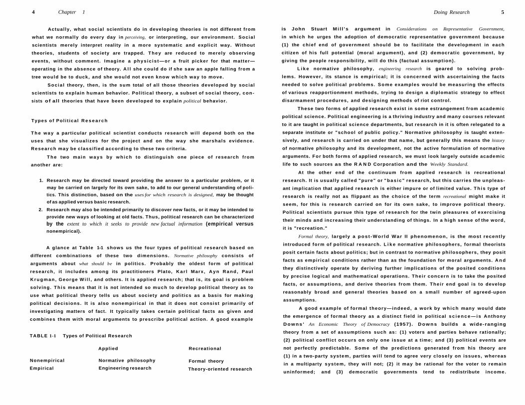
A glance at Table 1-1 shows us the four types of polit ical research based on

different combinations of these two dimensions. Normative philosophy consists of

arguments about what should be in poli t ics. Probably the oldest form of polit ical

research, i t includes among its practitioners Plato, K a r l Marx , A y n R a n d , Paul

K r u g m a n , George W i l l , and others. I t is applied research; that is , its goal is problem

solving. T h i s means that it is not intended so much to develop polit ical theory as to

use what polit ical theory tells us about society and polit ics as a basis for making

polit ical decis ions. It is also nonempir ical in that it does not consist pr imari ly of

investigating matters of fact. It typical ly takes certain poli t ical facts as given and

combines them with moral arguments to prescribe polit ical action. A good example

TABLE 1-1 Types of Political Research

Applied Recreational

Nonempirical

Empirical

Normative philosophy

Engineering research

Formal theory

Theory-oriented research

Doing Research 5

is John Stuart M i l l ' s argument in Considerations on Representative Government,

in wh ich he urges the adoption of democrat ic representative government because

(1) the chief end of government should be to facilitate the development in each

cit izen of his full potential (moral argument), and (2) democrat ic government, by

giving the people responsibil i ty, w i l l do this (factual assumption) .

L i k e normative philosophy, engineering research is geared to solving prob­

lems. However, its stance is empir ica l ; it is concerned with ascertaining the facts

needed to solve polit ical problems. S o m e examples would be measur ing the effects

of various reapportionment methods, trying to design a diplomatic strategy to effect

disarmament procedures, and designing methods of riot control.

These two forms of applied research exist in some estrangement from academic

political science. Polit ical engineering is a thriving industry and many courses relevant

to it are taught in political science departments, but research in it is often relegated to a

separate institute or "school of public policy." Normative philosophy is taught exten­

sively, and research is carried on under that name, but generally this means the history

of normative philosophy and its development, not the active formulation of normative

arguments. For both forms of applied research, we must look largely outside academic

life to such sources as the R A N D Corporation and the Weekly Standard.

At the other end of the cont inuum from applied research is recreational

research. It is usual ly cal led "pure" or " b a s i c " research, but this carries the unpleas­

ant implication that applied research is either impure or of l imited value. T h i s type of

research is really not as flippant as the choice of the term recreational might make it

seem, for this is research carried on for its own sake, to improve polit ical theory.

Polit ical scientists pursue this type of research for the twin pleasures of exercising

their minds and increasing their understanding of things. In a high sense of the word,

it is "recreation."

Formal theory, largely a post -Wor ld War II phenomenon, is the most recently

introduced form of polit ical research. L i k e normative phi losophers, formal theorists

posit certain facts about pol i t ics; but in contrast to normative phi losophers, they posit

facts as empir ical conditions rather than as the foundation for moral arguments. A n d

they distinctively operate by deriving further implicat ions of the posited conditions

by precise logical and mathematical operations. The i r concern is to take the posited

facts, or assumptions, and derive theories from them. The i r end goal is to develop

reasonably broad and general theories based on a smal l number of agreed-upon

assumptions.

A good example of formal theory—indeed, a work by w h i c h many would date

the emergence of formal theory as a distinct f ield in polit ical s c i e n c e — i s Anthony

D o w n s ' An Economic Theory of Democracy (1957) . D o w n s builds a wide-ranging

theory from a set of assumptions such as: (1) voters and parties behave rationally;

(2) polit ical confl ict occurs on only one issue at a t ime; and (3) poli t ical events are

not perfectly predictable. S o m e of the predictions generated from his theory are

(1) in a two-party system, parties w i l l tend to agree very c losely on issues, whereas

in a multiparty system, they w i l l not; (2) it may be rational for the voter to remain

uninformed; and (3) democratic governments tend to redistribute income.

6 Chapter 1

( O f course, one must recognize that excerpts such as these do even more than

the usual v io lence to a r ich net of theories.) It is important to emphasize that this sort

of work is almost solely an exercise in deduction. A l l of the conclusions derive

logical ly from a l imited set of explicit assumptions. D o w n s ' purpose in this is s imply

to see where the assumptions he started wi th w i l l lead h im. Presumably, if the

assumptions produced an untenable result, he would go back and reexamine them.

T h e main use of formal theory, as in the example above, is explanation; a

formal theory is used to construct a set of conditions f rom w h i c h the thing we w i s h

to explain would have logical ly f lowed. S u c h explanatory formal theories are then

often tested empir ical ly through theory-oriented research. But because formal theory

consists of taking a set of assumptions and working out where they lead—that is ,

what they logical ly i m p l y — i t is also useful for developing and analyzing strategies

for poli t ical action. That is , we can use formal theory to construct analyses of the

fol lowing form: If we want to achieve X, can we devise a set of reasonably true

assumptions and an action w h i c h , in the context of those assumptions, w i l l logical ly

lead to XI Fo rma l theory is used in this way, for example, to argue for various ways

to set up elections, or for various w a y s to arrange taxes so as to get the outcomes we

want. Flat-tax proposals are a good example: T h e y originated in argument of the

fol lowing form: (a) I f we want to max imize investment and economic growth, and

(b) if we assume that governmental investment is inefficient and that individual

taxpayers act so as to max imize their income, then (c) can we deduce what sort of

taxes in the context of the assumptions of (b) would best achieve (a)?

L i k e normative philosophy, formal theory interacts with empir ica l research.

Forma l theorists usual ly try to start with assumptions that are in accord with existing

knowledge about poli t ics, and at the end they may compare their f inal models with

this body of knowledge. B u t they are not themselves concerned with turning up new

factual information.

Good work in formal theory wi l l take a set of seemingly reasonable assumptions

and wi l l show by logical deduction that those assumptions lead inescapably to con­

clusions that surprise the reader. The reader must then either accept the surprising

conclusion or reexamine the assumptions that had seemed plausible. Thus , formal theory

provides insights by logical argument, not by a direct examination of political facts.

Fo l lowing from D o w n s , a great deal of formal theory in polit ical sc ience has

based itself on the economists ' core assumption of rational choice: the assumption

that individuals choose their actions in order to max imize some valued object, and

min imize the cost expended in achieving it. ( In economics the valued object is gen­

eral ly taken to be money; in polit ical sc ience it may be m o n e y — a s in theories of why

and how communit ies seek pork-barrel spending—but theories may also posit that

the valued object is a nonmonetary pol icy such as abortion, or poli t ical power itself.

Somet imes the object may even be left unspecif ied in the theory.)

A good example of formal theory that illustrates the rational choice assump­

tion is M a n c u r O l s o n ' s The Logic of Collective Action (1965) . T h e rational choice

assumption pointed O lson to a question no one had asked before, and al lowed h im to

stand received w i s d o m on its head. O l s o n wrote on the very basic question of

polit ical organization in society. Before his book, scholars had assumed that when

Doing Research 7

interests existed in soc ie ty—rac ia l minorit ies, businesses, professions, groups with

special concerns such as historic preservat ion—poli t ical organizations could be

expected to emerge naturally to represent those interests. 2 We should thus expect to

see a wide range of parties and interest groups engaged in poli t ics. A whole school of

political sc ience, the pluralist school, was organized around the expectation that

most of the time, most of society 's interests would be actively organized.

B a s e d on the rational choice assumption, however, O l s o n reasoned that there

was nothing natural about organization at a l l . F r o m the standpoint of any individual

in a group with a shared object, he concluded, participation in the group is usual ly

nonrational. R e m e m b e r that the rational choice assumption states that individuals

choose their actions in order to max imize a valued object, whi le min imiz ing the cost

expended in achieving it. If I am a person concerned with historic preservation,

I know that unless I have very unusual resources, my individual contribution to an

interest group pursuing preservation wi l l not make a measurable difference. L e t us

say there are 300,000 people around the country w h o share my interest; if each of us

contributes $ 100 to the cause, the difference if I do or do not contribute is a budget of

$29,999,900 versus $30,000,000. To the organization this amount would be trivially

smal l , but to me $100 makes a real difference. If I contribute, I w i l l have expended a

significant cost without getting any more of my valued good, w h i c h is not rational.

What is rational, instead, is to be a free rider, and let all those other people make the

contributions. However , O l s o n pointed out, s ince every potential member of such an

organization is in this same situation, the marvel should be that any interest organi­

zations exist at a l l .

O lson laid out several conditions under wi i ich organizations might nonetheless

arise. O n e such condition is that one potential member might have such large

resources that she knows no organization is possible without her participation. T h e

largest department store in town, for instance, knows that a Downtown Merchants '

Associat ion cannot function i f i t does not j o i n and contribute. T h e B i j o u x Tee-Shir t

Shop on the corner, though, is not in that situation. Under these c i rcumstances, we

can count on an organization being set up, because rationally, the large store cannot

get its valued good unless it takes the lead in setting up the associat ion.

No theory can ever be a l l -encompassing, and in fact one function of theory

may be that it highlights exceptions for closer examination. We know that many

people do contribute to polit ical organizations even though, as O l s o n has proved, it is

irrational for them to do so. T h e virtue of O l s o n ' s theory in this case is that instead of

v iewing such contributions as "natural" and therefore ignoring them, we are forced

to treat the contributions as a puzzle requiring further investigation.

However, in a wide array of settings Olson 's theory predicts behavior rather wel l .

The excruciating efforts of public television stations to get their viewers to jo in rather

than be free riders ("Please! On ly one in ten of our viewers is a member. If you jo in

K X X X - T V today we wi l l send you this beautiful coffee mug!") bears testimony to the

power of Olson 's logic. In the next chapter you wi l l see that it may also help to explain

why small nations typically do not pull their "fair" weight in international alliances.

2 For example, Duverger (1963) assumed this in the theory I described on pp. 2 - 3 .

8 Chapter 1

Although formal theory is the fastest growing type of polit ical research, most

research and teaching in poli t ical sc ience is stil l of the fourth type suggested in

Table 1-1, theory-oriented research. T h i s type of research is concerned with

expanding our knowledge of what happens in polit ics and of w h y it happens as it

does. L i k e poli t ical engineering, i t is empir ica l ; i t is concerned with discovering facts

about poli t ics. But unl ike engineering, w h i c h deals with facts only for their useful ­

ness in specif ic pol i t ical problems, this research deals with them to develop new

polit ical theories or to change or conf i rm old ones. Accord ing ly , the most important

activity in this research is the development of theories l inking observed facts about

polit ics. In engineering, facts are sought out if they are needed to solve a problem;

here they are sought out if they w i l l be useful in developing theories.

Duverger 's study of poli t ical parties is an example of theory-oriented research.

Another good example is a test by D i e h l and K ingston (1987) of the theory that arms

buildups lead to mil i tary confrontations. T h e y examined changes in military expen­

diture by major powers from 1816 to 1976 to see whether increases tended to be

fol lowed by involvement in war. No matter how they adjusted th ings—look ing for

delayed reactions, looking only at "arms races" in w h i c h two rivals simultaneously

increased their military forces, and so on—they found no relationship. Mi l i tary

engagements were no more or less l ikely to occur fol lowing military buildups than

under other c i rcumstances. T h e y concluded by exploring the implicat ions of this

f inding, one of w h i c h is that arms expenditure must therefore be determined more by

domestic poli t ical considerations than by the international situation.

R e s e a r c h M i x

Pract ical ly no research is a pure example of any of the types I have presented here.

T h e s e are abstract distinctions, types of emphasis found in particular pieces of

research. General ly , any specif ic piece of work is a mix of more than one of the

types. A l though one method w i l l usual ly predominate, there w i l l almost a lways be

some interaction between the different types in any given work. T w o examples may

help illustrate this point.

F i rst , let us look a bit more c losely at normative philosophy, using K a r l Marx 's

work as an example. M a r x ' s theory of the dialectic is pr imari ly a work in normative

philosophy. H i s argument takes the same general form as that in M i l l ' s essay on rep­

resentative government: " B e c a u s e aspects of the human condition today are

bad, and because the state and the economy function in w a y s to produce these

bad effects, we should strive to change the state and the economy in ways ,

w h i c h w i l l el iminate the bad effects." B u t Marx was less wi l l ing than Mi l l to simply

assume the factual portions of his argument. Instead, he spent years of research

trying to work out the precise economic effects of capita l ism.

It should be evident that anyone developing normative theories about pol i t ics

must begin wi th some factual assumpt ions. A researcher may be relat ively more

wi l l ing to assume these facts f rom general exper ience and/or f rom the research

of others, as M i l l w a s ; on the other hand, he may w i s h , l ike M a r x , to conduct a

Doing Research 9

personal investigation of this factual bas is . S u c h activity w i l l , o f course , involve

h i m to some degree in engineering research . I t is character ist ic of normative

phi losophy, however , that the researcher need not feel required to produce the ful l

factual basis for h is argument. In this respect normative ph i losophy differs f rom

the empir ica l types of pol i t ical research.

T h e distinction is an important one. F o r one thing, the fact that normative

philosophers are not required to provide evidence for al l their assumptions leaves

them free to devote more energy to other parts of the research task. More important,

they often need to assume facts that cannot possibly be tested against reality. T h e

normative phi losopher must be free to imagine realities that have never existed

before, and these, of course, cannot be "tested." I f normative philosophers were held

to the same standards of factual evidence as empir ical researchers, al l U t o p i a n

dreams would have to be thrown out.

As a second example of the w a y in w h i c h types of research are mixed in any

one work, let us look at a case in w h i c h researchers work ing on a primari ly engi­

neering project found they had to develop a theory to make sense out of their work.

A group of sociologists led by Samuel Stouffer was employed by the A r m y to study

the morale of A m e r i c a n soldiers during World War I I (Stouffer and others, 1949).

Stouffer and his coworkers were puzz led by the fact that often a soldier 's morale had

little to do with his objective situation.

For instance, M P s were objectively less l ikely to be promoted than were members

of the A r m y A i r Corps. Of Stouffer's sample of M P s , 24 percent were noncommis­

sioned officers ( N C O s ) , compared with 47 percent of the air corpsmen. Paradoxically,

however, the M P s were much more likely than the air corpsmen to think that soldiers

with ability had a good chance to advance in the Army. Th is sort of paradox occurred a

number of times in their study, and the researchers felt they had to make some sense of

it if their efforts were to help the A r m y improve morale.

They did this by developing the theory of relative deprivation to account for

their seemingly contradictory f indings. Accord ing to this theory, satisfaction with

one's condit ion is not a function of how wel l -of f a person is objectively, but of

whether her condit ion compares favorably or unfavorably with a standard that she

perceives as normal .

T h e fact that so many air corpsmen were N C O s apparently made the corpsmen

feel that promotion was the normal thing. T h o s e who were not promoted were disap­

pointed, and those w h o were promoted did not feel particularly honored. A m o n g the

M P s , on the other hand, promotion was sufficiently infrequent that not being pro­

moted was seen as the norm. T h o s e who were not promoted were not disappointed,

and those who were promoted felt honored. T h u s , paradoxical ly, the air corpsmen,

who were more l ikely to be promoted, felt that chances for promotion in the A r m y

were poor, and the M P s , w h o were less l ikely to be promoted, felt that chances for

promotion in the A r m y were good!

I have mentioned these two examples to illustrate my point that most research

work involves some mix of the four types of research. Indeed, a mix is so much the

usual situation that when I tried to make a rough head count of the frequency of the

10 Chapter 1

different types of research in poli t ical science journals , I was unable to do so. I was

s imply unwi l l ing to assign most articles to one or another of the categories. It is just

not often the case that a researcher can easi ly be labeled a normative philosopher, an

engineer, a formal theorist, or a theory-oriented empir ica l researcher. These types

interact in the work of every polit ical scientist.

That most research involves a mix of the types does not preclude the impor­

tance of the distinctions, however. General ly , one type of research is dominant in any

given piece of work, depending on the goals of the researcher. T h e s e goals have a lot

to do with the w a y a study should be set up and the criteria according to w h i c h it

should be judged.

E v a l u a t i n g D i f fe ren t Types o f R e s e a r c h

It is dangerous to set down simple standards for good research. L i k e any creative

work, research should be evaluated subjectively, according to informal and rather

f lexible criteria. B u t I w i l l r isk suggesting two standards for research that wi l l serve

as examples of the w a y in w h i c h the type (or types) of research we are doing dictates

the w a y we should conduct that research.

In the first p lace, in either form of empir ical research, the researcher should be

held responsible for demonstrating the factual basis of his conclusions. In either

form of nonempir ical research, this is not necessary, although a normative argument

may be made more convinc ing, or an exercise in formal theory may be made more

interesting, by providing evidence for the factual basis on w h i c h its assumptions rest.

In the second place, good research of any sort should be directed to an inter­

esting problem. B u t what sort of problem is "interesting" depends largely on the

motivation of the study. F o r either sort of applied research, problems should be

chosen wh ich are of real importance for contemporary policy. Today, an argument

about c iv i l disobedience, for example, makes a more interesting problem in norma­

tive theory than a problem dealing with an argument about dynast ic success ion; a

few hundred years ago the reverse would probably have been the case. In other

words, applied research should be relevant, in the common usage of the word.

Recreat ional research, on the other hand, requires problems that wi l l have a

substantial impact on existing bodies of theory. M a n y topics that are of considerable

importance to an engineer show little promise for theory-oriented research.

Simi lar ly , many promising topics for recreational research are not directly relevant.

F o r example, research on the difference between men 's and women 's voting in

Ice land in the 1920s and 1930s would sound absurd f rom the standpoint of an

engineer. B u t these voting patterns, occurr ing just after the extension of the vote to

women, might be important for theories of how voting patterns become established

among new voters. H o w to choose an interesting problem is one of the most difficult

and chal lenging parts of empir ical research. I w i l l d iscuss this in some detail in

Chapter 2.

In general , this book is concerned with empir ical research. Within empir ical

research, I devote somewhat more attention to theory-oriented research than to

Doing Research 11

engineering. There are two reasons for this: (1) It is the more common kind of

research in pol i t ical sc ience, and (2) it poses rather more difficult instructional

problems than does engineering.

E T H I C S O F P O L I T I C A L R E S E A R C H

Conduct ing research is an act by you. Y o u must therefore be concerned about the

ethics of your research, just as you are with all of your actions. There are two broad

classes of ethical questions regarding our research. F i rst , we must concern ourselves

with the effects on society of what we discover. F o r instance, if you study techniques

of polit ical persuasion, it is possible that what you learn could be used by a polit ical

charlatan to do bad things. A col league once publ ished a study of the effects of

electoral systems on representation, only to learn later that it was used by a military

junta in a La t in A m e r i c a n country to figure out how to produce a controllable

"democracy."

A l s o , the results of a research can be demeaning or dehumaniz ing. Recent

results in psychology suggesting that a wide range of behaviors are genetically con­

trolled go against our prevail ing disposit ion to think of humans as free agents in what

they do. R e s e a r c h on racial or ethnic groups is particularly sensit ive, as we may fear

that innocent research results might reinforce preexisting stereotypes.

E t h i c a l quest ions of this sort are espec ia l l y diff icult because the results of

our research are so hard to predict. Another co l league, in b io logy, was upset w h e n

he learned that h is research on f rogs ' eyes turned out to have appl icat ions in the

design of gu idance systems for m i s s i l e s ! In the case of demeaning or dehumaniz ­

ing research , a further prob lem ar ises , in that what seems " d e h u m a n i z i n g " to a

person depends on what the person thinks " h u m a n " m e a n s — t h a t is , i t is very

much a matter of personal bel iefs and cul tural context. T h e p s y c h o l o g i c a l

research noted above may s e e m w h o l l y appropriate, for ins tance , depending on

one's v iew of h u m a n n e s s . As another example , the theory of evolut ion appears

dehumaniz ing to many fundamental ist Chr is t i ans but does not appear so to many

other people.

O n e response to such difficulties might be to take a "pure sc ience" approach,

arguing that because it is so hard to judge the results of knowledge anyway, we

should let the chips fall where they may. We should s imply seek truth and not worry

about its effects. As we wi l l see throughout this book, however, the socia l scientist

rarely deals in unquestioned truths. We work under sufficient diff iculties, especial ly

the fact that we usual ly cannot operate by experimentation (see Chapter 6 ) , that our

results are to some extent a subjective interpretation of reality. We operate within

rules of evidence in interpreting reality, so we are constrained in what we can assert

and cannot s imply pul l f indings out of a hat; but still our results involve individual

choices and judgment by us. We are not s imply neutral agents of truth; we must take

personal responsibil i ty for the results of our research, difficult though these ethical

questions may be.

12 Chapter 1

A second class of questions, more specific than the ones described earlier but not

necessari ly easier to answer, deals with our treatment of the people we are studying.

We are responsible to treat the subjects of our study fairly and decently. Particular

problems arise in the fol lowing ways:

1. Harm to subjects. Harming the subjects of your study, either by doing harmful things to

them or by withholding good things from them, should generally be avoided. Is it

ethically right, for example, in evaluating the effects of a program to get people off the

welfare rolls and into jobs, to withhold the program from some deserving people while

administering it to others, in order to see how effective it is?

2. Embarrassment or psychological stress. You should avoid shaming people into partici­

pating in your study, or submitting them to embarrassing situations.

3. Imposition. You are asking your subjects to help you. Don't demand more of them than

is reasonable. Public officials may get a hundred questionnaires a year; keep yours

short. Dinnertime is a good time to reach people by phone, but it is also an annoying

time if you have 15 minutes' worth of questions to ask.

4. Confidentiality. Generally, the subjects of your study will wish to have their privacy

protected. It is not enough just to withhold publishing their names. Relevant details you

include in your report might make it easy to identify the subject (a member of

Congress, female, from the South, the senior member of her committee). You should

take care to truly mask the subjects who have helped you.

5. Fooling or misleading the subjects. As an overall rule, you should make certain that

your subjects know exactly what they will be doing and what use you will make of

them. As you will see in Chapter 6, the results of your study might well be more valid

if the people you study are unaware that they are being studied. However, everyone has

the right not to be fooled and not to be used without his or her consent.

T h e problems I have noted here pose difficult ethical questions of the "ends

and means" sort. If a research that w i l l benefit society can be conducted only by

mistreating subjects, should it be done? There is no clear answer. If the costs to sub­

jects are slight ( inconvenience, pain of w h i c h they are informed in advance) and the

social benefits great, we would generally say yes , it should be done. But what if i t

puts subjects in danger of death, as may be true of polit ical research that delves into

racketeering or corruption?

T h e most horrible historic example of science gone bad is that of the Naz i

doctors w h o ki l led prisoners by immers ing them in ice water to see how long people

could survive in freezing water. A painful ethical question today is whether even to

use the results of that research, w h i c h was purchased at great human pain, but w h i c h

may potentially help in saving l ives a n d — w e h o p e — w i l l never be available again

from any source. D o e s using the results of the research just i fy it? I f so, perhaps we

should destroy the results. But might that not lead to greater human pain for v ict ims

of freezing and exposure w h o m we might have helped?

T h e one f irm rule, for me at least, is that people should never be coerced or

tricked into participation and should a lways be fully informed before they agree to

participate.

In this chapter we look more c losely at the nature of polit ical theories and at the fac­

tors that inf luence the decision to do research on a particular theory. A l o n g the way

I wi l l d iscuss some standards to use in deciding whether a theory is weak or strong.

Al though this chapter deals with poli t ical theories, you should not assume that

it is important only for what I have ca l led theory-oriented research. Indeed, as I

pointed out in Chapter 1, the key to solv ing many engineering problems may be a

polit ical theory of some sort. To effect a change in some given phenomenon, you

may need to develop a theory that accounts for several factors and al lows you to

manipulate them to produce the desired change. M u c h applied research on the prob­

lem of enriching the education of underprivi leged chi ldren, for example, has had to

concern itself with developing theories to explain why one chi ld learns things more

quickly than another. T h e Stouffer study, cited in Chapter 1, is another example of an

engineering study in wh ich it was necessary to develop a theory. In that case,

Stouffer and his collaborators had to explain w h y M P s had higher morale than air

corpsmen. T h i s was necessary if they were to devise w a y s to raise the morale of

A r m y personnel in general.

On the other hand, many engineering studies do not require that a theory be

developed; they simply involve measur ing things that need to be measured. Taking

the U . S . census is one example of such engineering research. Others include the

Gal lup Po l l , studies measuring the malapportionment of state legislatures, and c o m ­

parisons of the relative military strength of various countries.

In s u m , engineering research may or may not involve the development of

polit ical theories; theory-oriented research a lways does. Theory is a tool in one type

of research; it is an end in itself in the other. But no matter w h i c h type of research

one is currently engaged in , it is worth taking a closer look at the nature of theory.

13

14 Chapter 2

C A U S A L I T Y A N D P O L I T I C A L T H E O R Y

In the socia l sc iences, theories generally are stated in a causa l mode: "I f X happens,

then Y w i l l fol low as a result." T h e examples we looked at in Chapter 1 were all of

this form. In the Duverger example, i f a certain configuration of polit ical confl icts

exists, and if the country adopts a certain electoral law, then the number of polit ical

parties in the country can be expected to grow or shrink to a certain number. In the

D i e h l and K ingston study, the authors tested a theory that if a country increases its

military expenditure, then it might be expected to go to war.

A causal theory a lways includes some phenomenon that is to be explained or

accounted for. T h i s is the dependent variable. In Duverger 's theory, the dependent

variable was the number of parties. A causal theory also includes one or more factors

that are thought to affect the dependent variable. T h e s e are cal led the independent

variables. Duverger used two independent variables in his theory: the nature of

social confl icts in a country and the country 's electoral system.

A l l of these factors are cal led "var iables" s imply because it is the variation of

each that makes it of interest to us. If party systems had not var ied—that is , if each

country had had exactly the same number of part ies—there would have been nothing

for Duverger to explain. If one or the other of his independent variables had not

varied, that factor would have been useless in explaining the dependent variable. F o r

instance, if all countries had had the same electoral system, the variations in party

systems that puzz led h im could not have been due to differences in the countries'

electoral systems, inasmuch as there were no differences.

T h e dependent variable is so named because in terms of the particular theory

used it is thought to be the result of other factors (the independent variables) .

T h e shape it takes "depends" on the configuration of the other factors. S imi lar ly , the

independent variables are thus designated because in terms of the particular theory,

they are not taken as determined by any other factor used in this particular theory.

T h e same variable may be an independent variable in one theory and a

dependent var iable in another. F o r instance, one theory might use the soc ia l status

of a person 's father (the independent var iable) to expla in the person's soc ia l status

(the dependent var iable) . Another theory might use the person 's socia l status as an

independent var iable to expla in something e lse , perhaps the w a y the person votes.

T h u s , no variable is innately either independent or dependent. Independence

and dependence are the two roles a variable may play in a causal theory, and it is not

something about the variable itself. It all depends on the theory:

Theory 1: Democracies do not tend to initiate wars.

Theory 2: Countries with high per capita incomes are more likely to be democracies

than poor countries are.

In theory 1, democracy functions as an independent variable; the tendency to wage war

depends on whether or not a country is a democracy. In theory 2, democracy functions

as a dependent variable; whether or not a country is l ikely to be a democracy depends

on its per capita income.

Political Theories and Research Topics 15

W H A T D O E S G O O D T H E O R Y L O O K L I K E ?

Three things are important if we are to develop good, effective theories:

1. Simplicity. A theory should give us as simple a handle on the universe as possible.

It should use no more than a few independent variables. It would not be very useful to

develop a theory that used 30 variables, in intricate combinations, to explain why

people vote the way they do. Such a theory would be about as chaotic and as difficult

to absorb as the reality it sought to simplify.

2. Predictive accuracy. A theory should make accurate predictions. It does not help to

have a simple, broad theory which gives predictions that are not much better than one

could get by guessing.

3. Importance. A theory should be important. However, what makes a theory important is

different in engineering research than in theory-oriented research, so we shall consider

them separately.

In engineering research, a theory should address a problem that is currently

pressing. T h i s is a subjective judgment, of course, but before you begin your

research, you should try to justi fy your choice of topic, not only to yoursel f but also

to your audience. Your research report should include some d iscussion of the impor­

tance of the problem and of possible applications for your f indings. I t may seem

unnecessary to point this out, but it is an important part of the engineering research

project, one that is often carried out sloppi ly and in an incomplete way. Students

have been known, for example, s imply to turn in a computer printout as a paper,

because "the applications are obvious." True , the obvious applications are obvious,

but an imaginative researcher w h o sits down and thinks about it for awhile may be

able to point up additional, more varied ways in w h i c h the results can be used.

In theory-oriented research, the theory should give a handle on as big a portion

of the universe as possible; that is , it should apply broadly and generally. It is easy to

develop a trivial theory. A theory of the organization of borough presidencies in New

York Ci ty , for example, might predict quite accurately for that specif ic situation. B u t

inasmuch as the borough presidents have little power, it would not help us very

much to reduce the chaos of N e w Y o r k C i ty poli t ics, let alone the chaos of polit ics in

general.

W h e n we say that a theory should apply "broadly" and "generally," we are

referring not only to how large a selection of items from reality the theory deals with,

but also to how great a variety of preexisting theories are affected by the new theory.

A theory can attain great generality rather economical ly if it helps to recast older the­

ories, each of w h i c h involves its own portion of reality. T h u s , a theory of electoral

change might take on importance partly from the phenomena it explained d i rec t l y—

changes in people's votes; but it wou ld be a more valuable tool if it could be shown

to have significant implicat ions for other areas of socia l theory—democrat ic theory,

general theories of attitude change, or whatever. In effect, it would perform two s i m ­

plifying functions: It would not only give us a handle on the rather l imited portion of

our environment that it sought to explain directly, but it would also shed light on the

wider universe dealt with by the other theories.

16 Chapter 2

In the example jus t c i ted, a theory to expla in the organization of borough

presidencies in N e w York , the theory accrues so little importance direct ly as to

look absurd. B u t i t might be poss ib le , i f the borough pres idencies were taken

as examples of some broader concept in urban pol i t ics, that the study wou ld bor­

row importance f rom this under ly ing phenomenon. T h e borough presidencies

might, for example , serve as a usefu l m i c r o c o s m for studying the work ings of

patronage.

If a theory can succeed reasonably wel l at meeting these three c r i t e r i a—

importance, simplicity, and predictive a c c u r a c y — i t w i l l be useful as a tool for

s impl i fy ing reality. S u c h a theory is sometimes described as elegant.1 One difficulty

in creating an elegant theory is that trying to meet any one of the three basic criteria

tends to make it harder to meet the other two. In the example of Duverger 's theory,

we saw that he might have improved the accuracy of his theory's predictions by

bringing in additional explanatory variables; but this wou ld have reduced the

simplici ty of the theory. Simi lar ly , an attempt to make a theory more general often

w i l l cost us something in either the simpl ic i ty of the theory or the accuracy of its

predictions.

A s i d e f rom its utility and simplicity, there is also an element of "beautiful

surprise" to elegant research. A piece of research that goes against our expectations,

that makes us rethink our world, gives us a special k ind of pleasure. Pol i t ical scientists

often jok ingly refer to this element as the "interocular subjectivity test" of r e s e a r c h —

Does it hit us between the eyes?

A good example of research with beautiful surprise is a study of the impact of

"get-tough" pol ic ies against i l legal immigrat ion across the Uni ted S t a t e s - M e x i c a n

border. In the late 1980s and early 1990s, the U . S . Immigrat ion and Natural ization

Serv ice added extra guards and imposed punishments on employers found to be

hiring i l legal immigrants. O n e thousand extra border patrol officers were then added

each year for several years afterward. Douglas S . M a s s e y and Kr is t in E . E s p i n o s a

(1997) found that s ince the border crossing had been made tougher, i l legal i m m i ­

grants who originally would have come to the Uni ted States for only a few months of

seasonal labor now stayed year-round because they knew it would be hard to get

back into the Uni ted States if they went home to M e x i c o . T h e end result was that the

number of i l legal immigrants present at any given time was increased, not decreased,

by the stepped-up enforcement.

I t appears to be part icular ly hard to ach ieve elegant research in the soc ia l

s c i e n c e s , compared wi th other sc ient i f ic areas. H u m a n behavior is more complex

than the behavior of p h y s i c a l o b j e c t s — i n fact, s o m e think i t may perhaps be

largely beyond explanat ion. On the other hand, i t may be that h u m a n behavior can

be understood, but that we have not yet c o m e up wi th a soc ia l theory that cou ld

show the true potential of our f ie ld. At any rate, i t is rare for theory in the soc ia l

sc iences to ach ieve e legance. If a theory 's predict ions are reasonably accurate , i t

'The choice of this word typifies the aesthetic pleasure—and the vanity—with which researchers approach their work.

Political Theories and Research Topics 17

is usua l ly because the scope of the theory is restricted or because many of the

exceptions to the theory have been absorbed into it as addit ional var iab les ,

making i t very c o m p l e x . 2

T h e fact that most social science theory is not very elegant does not mean that it

is not good. T h e real test of a theory's value is whether its subject matter is important

and how close it has come to elegance, given that subject matter. If it is important to

understand humankind's behavior, it is important to try to develop theories about it,

even if things do not fall as neatly into place as we would l ike.

1 am a lways amused when people say of a question that is being made to look

more difficult than it real ly is , " T h i s shouldn't be that hard; what the heck, it's not

rocket s c i e n c e " — i m p l y i n g that rocket science is the essence of difficulty and

complexity. Not to take away from the difficulty of rocket sc ience, but plotting the

trajectory of an object in a vacuum is far simpler than understanding the motivation

of a human being. Perhaps one day the old saw wi l l become, " T h i s shouldn't be that

hard; what the heck, it's not social sc ience."

E x a m p l e o f E legan t R e s e a r c h : Ph i l ip C o n v e r s e

In his article " O f T i m e and Partisan Stabil i ty" (1969) , Phi l ip Converse came about

as close to developing an "elegant" theory as one can commonly do in the socia l

sciences. H i s study is worth looking at in some detail.

Converse took as his dependent variable the strength of the "party identification"

of individuals—their sense that they are supporters of one or another of the political

parties. In an earlier study, he and Georges Dupeux had found that, whereas about

75 percent of Amer icans who were polled identified with some political party, a s imi ­

lar poll conducted in France showed that less than 45 percent of the respondents did

so (Converse & Dupeux, 1962). Other studies had shown high levels of party identifi­

cation in Britain and Norway, and lower levels of party identification in Germany and

Italy. Because the overall extent to which citizens of a particular country felt bound to

the existing parties seemed likely to have something to do with how stable politics in

that country would be, Converse wanted to know w h y the level of party identification

varied as it did from country to country.

At the time of their earl ier study, he and D u p e u x had found that the difference

in percentage of party identifiers between F rance and the Uni ted States seemed to

be explained almost who l ly by the fact that more A m e r i c a n s than F r e n c h had some

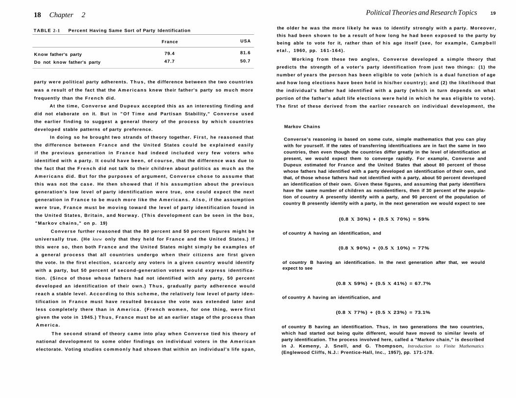
idea of what party their fathers had identif ied with. As we can see in Table 2-1,

within each row there was pract ical ly no difference between the F r e n c h

and A m e r i c a n levels of party identif ication. In both countries about 50 percent of

those who did not know their father's party expressed identif ication with

some party themse lves . 3 About 80 percent of those w h o did know their father's

2 Another reason for the difficulty of attaining elegance in social research is simply that most social science terms are imprecise and ambiguous. This problem is addressed in Chapter 3.

3 Remember that this was an early study, done in 1962. It was not long before further work showed similar effects for mothers!

18 Chapter 2

TABLE 2-1 Percent Having Same Sort of Party Identification

France USA

Know father's party 79.4 81.6

Do not know father's party 47.7 50.7

party were pol i t ical party adherents. T h u s , the difference between the two countries

was a result of the fact that the A m e r i c a n s knew their father's party so m u c h more

frequently than the F r e n c h did.

At the t ime, Converse and Dupeux accepted this as an interesting finding and

did not elaborate on it. But in " O f T i m e and Partisan Stability," Converse used

the earlier f inding to suggest a general theory of the process by w h i c h countries

developed stable patterns of party preference.

In doing so he brought two strands of theory together. F i rs t , he reasoned that

the difference between F r a n c e and the Un i ted States cou ld be expla ined easi ly

i f the previous generation in F r a n c e had indeed inc luded very few voters w h o

identif ied with a party. It cou ld have been, of course , that the difference was due to

the fact that the F r e n c h did not talk to their chi ldren about pol i t ics as m u c h as the

A m e r i c a n s did. B u t for the purposes of argument, C o n v e r s e chose to assume that

this was not the case . He then showed that i f h is assumpt ion about the previous

generat ion's low level of party identif ication were true, one could expect the next

generation in F r a n c e to be m u c h more l ike the A m e r i c a n s . A l s o , i f the assumpt ion

were true, F r a n c e must be mov ing toward the level of party identif icat ion found in

the Un i ted States, Br i ta in , and Norway . ( T h i s development can be seen in the box,

" M a r k o v cha ins ," on p. 19)

Converse further reasoned that the 80 percent and 50 percent figures might be

universal ly true. (He knew only that they held for F r a n c e and the Uni ted States.) If

this were so, then both F rance and the Uni ted States might s imply be examples of

a general process that al l countries undergo when their c i t izens are first given

the vote. In the first e lect ion, scarcely any voters in a given country would identify

with a party, but 50 percent of second-generat ion voters would express identif ica­

tion. (S ince of those whose fathers had not identified wi th any party, 50 percent

developed an identif ication of their own.) T h u s , gradually party adherence would

reach a stable level . A c c o r d i n g to this scheme, the relatively low level of party iden­

tif ication in F r a n c e must have resulted because the vote w a s extended later and

less completely there than in A m e r i c a . (F rench w o m e n , for one thing, were f i rst

given the vote in 1945.) T h u s , F r a n c e must be at an earl ier stage of the process than

A m e r i c a .

T h e second strand of theory came into play when Converse tied his theory of

national development to some older findings on individual voters in the A m e r i c a n

electorate. Voting studies commonly had shown that within an individual 's l ife span,

Political Theories and Research Topics 19

the older he was the more l ikely he was to identify strongly with a party. Moreover,

this had been shown to be a result of how long he had been exposed to the party by

being able to vote for it, rather than of his age itself (see, for example, Campbe l l

e ta l . , 1960, pp. 161 -164 ) .

Work ing f rom these two angles, Converse developed a simple theory that

predicts the strength of a voter's party identification from just two things: (1) the

number of years the person has been eligible to vote (wh ich is a dual function of age

and how long elections have been held in his /her country) ; and (2) the l ikel ihood that

the individual 's father had identified with a party (wh ich in turn depends on what

portion of the father's adult life elections were held in w h i c h he was el igible to vote).

The first of these derived from the earlier research on individual development, the

Markov Chains

Converse's reasoning is based on some cute, simple mathematics that you can play with for yourself. If the rates of transferring identifications are in fact the same in two countries, then even though the countries differ greatly in the level of identification at present, we would expect them to converge rapidly. For example, Converse and Dupeux estimated for France and the United States that about 80 percent of those whose fathers had identified with a party developed an identification of their own, and that, of those whose fathers had not identified with a party, about 50 percent developed an identification of their own. Given these figures, and assuming that party identifiers have the same number of children as nonidentifiers, then if 30 percent of the popula­tion of country A presently identify with a party, and 90 percent of the population of country B presently identify with a party, in the next generation we would expect to see

(0.8 X 30%) + (0.5 X 70%) = 59%

of country A having an identification, and

(0.8 X 90%) + (0.5 X 10%) = 77%

of country B having an identification. In the next generation after that, we would expect to see

(0.8 X 59%) + (0.5 X 41%) = 67.7%

of country A having an identification, and

(0.8 X 77%) + (0.5 X 23%) = 73.1%

of country B having an identification. Thus, in two generations the two countries, which had started out being quite different, would have moved to similar levels of party identification. The process involved here, called a "Markov chain," is described in J. Kemeny, J. Snell, and G. Thompson, Introduction to Finite Mathematics

(Englewood Cliffs, N.J.: Prentice-Hall, Inc., 1957), pp. 171-178.

20 Chapter 2

second from his and D u p e u x ' s comparative study of F rance and the Uni ted States.

T h u s , essential ly, party identification is predicted f rom the individual 's age and the

length of t ime that the country has been holding elections.

A few examples of predictions from his theory are (1) at the time elections are

first held in a country, the pattern we typical ly observe in Europe and A m e r i c a (the

young being weakly identified, the old strongly) should not hold; all should identify

at the same low levels; (2) if elections were interrupted in a country (as in G e r m a n y

from 1933 to 1945) , levels of party identification should decl ine at a predictable rate;

(3) ( /the transition rates for al l countries were roughly the same as for F rance and the

Uni ted States, then party identification levels in al l electoral democracies should

converge over the next few generations toward a single value of about 72 percent.

Thus , although Converse's theory was quite simple, it was applicable to a wide

variety of questions. It simultaneously explained individual behavior and characteristics

of political systems. It implied a more or less universal form of political development

at the mass level—with a prediction of initial, but rapidly decreasing, potential for

electoral instability in a new electorate. A n d it included the startling suggestion of a

convergence of "mature" electorates to a common level of party identification approxi­

mately equal to that of Britain, Norway, or the United States.

T h e theory was simple, and it was broadly applicable. What was more, i t

seemed to predict fairly accurately, thus fulf i l l ing the third criterion for "elegance."

U s i n g data from Br i ta in , Germany, Italy, the Uni ted States, and M e x i c o to test the

theory, Converse found that the theory predicted quite wel l for al l five countries.

O v e r the years after it appeared, the Converse article stimulated a great deal of

further research, w h i c h is what one would expect of elegant work. H i s f indings

served as assumptions for formal theoretic work (Przeworski , 1975). They also st im­

ulated researchers to investigate whether in fact the transition probabilit ies on w h i c h

the Markov chain is based are the same in all industrial ized countries (Butler &

Stokes, 1969, p. 53) , and to test whether new electorates actually behave as

Converse 's theory predicts they would (Shively , 1972; Leitner, 1997; T i l ley , 2003;

Dal ton & Weldon, 2007) . It is in this way that a good piece of theoretical work feeds,

and becomes enmeshed in, the whole body of theoretical exploration.

To Q u a n t i f y o r N o t

A side issue in the question of how to develop elegant theory is the old chestnut:

Should political science be "quantitative" or not? There has been much rhetoric spilled

over this. As long ago as 1956, James Prothro cal led the dispute "the nonsense fight

over scientific method," but it has not cooled sufficiently in the intervening years.

It is a bit hard to pin down what the term quantitative means, but generally,

research that pays a good deal of attention to numerical measures of things, and

tends to make mathematical statements about them, is considered quantitative.

Research that is less concerned with measuring things numerical ly , and tends to

make verbal statements about them, is considered relatively less quantitative.

Political Theories and Research Topics 21

A n y t h i n g in pol i t ical sc ience can be stated with vary ing degrees of quantif i ­

cation. To give a crude example: " T h e length of serv ice of members of the U . S .

House increased f rom 1880 to 2005 on the average by 0.78 years every decade; the

rate of increase w a s 0.68 years per decade before 1922, and 0.86 years per decade

after 1922," says approximately the same thing as " F r o m 1880 to 2 0 0 5 , represen­

tatives served a steadily increas ing length of t ime in the House ; the change

proceeded a bit more rapidly in the latter ha l f of that per iod." T h e first form of the

statement gives more prec ise informat ion, but the sense of the two statements is

the same.

E a c h approach involves costs and benefits for research. M o s t people wou ld

agree that precise information is more useful than imprec ise information, al l other

things being equal . But it may be that the time and attention spent in gathering

precise data make it difficult for the researcher to appreciate the larger aspects of a

theory. A l s o , because some kinds of data by their very nature are more amenable to

precise formulat ion, there is the danger that overconcern with precis ion may restrict

our choice of research to those variables we can more easi ly quantify. I t is str iking,

for instance, how little the U . S . presidency is studied by pol i t ical scientists. T h i s

oversight may we l l be due to the difficulty of getting "hard" data on what goes on in

that office.

I deal with the issue of proper levels of precision in Chapter 5. F o r our purpos­

es here, the important thing is to see what relationship degrees of quantification bear

to elegance in research.

F i r s t of a l l , the part icular subject we are studying affects the extent to w h i c h

it is poss ib le for us to quantify. In e lect ion studies, there is cons iderab le scope for

quanti f icat ion. R e c o r d s f rom earl ier e lect ions are usua l ly kept in fa ir ly good

order; the results of many attitude surveys are a lso avai lable , and most voters do

not regard their act ions as something about w h i c h they need to mainta in secrecy .

T h u s , the quantitative researcher is able to do a great dea l . On the other hand,

in C h i n e s e studies, or in studies deal ing wi th the U . S . pres idency, sources of

quantitative data are quite restr icted, and most research must be relat ively non -

quantitative.

In virtual ly every f ield of polit ical research, however, work can be conducted

in either a pr imari ly quantitative or a primari ly nonquantitative mode. It is probably

best that studies with varying degrees of quantification be carried on in any given

field of poli t ical research, for the different levels of quantification complement each

other. Typica l ly , less quantitative research provides greater breadth, greater openness

to totally new theories, and a greater awareness of the complexi ty of social phenom­

ena. Studies employing more quantitative data, however, are more l ikely to produce

simple, usable theories; and they are certainly more l ikely to give us a c lear idea of

how accurate a theory's predictions are. T h u s , each approach has its own costs and

benefits, and it is we l l to remember that no particular degree of quantification has a

corner on elegance.

22 Chapter 2

C H O I C E O F A T O P I C

T h e choice of a research topic is intimately bound up with the elegance of what

comes out of the research effort. In selecting a topic, of course, the first step is to

choose a general area that is interesting and significant for you. By choosing to study

polit ical sc ience you have already begun to narrow the f ield, and you certainly wi l l

narrow things more before you are ready to begin. There is no difficulty in this; you

simply fol low your interests.

But once you have chosen a general area to work in, p icking a particular topic

to research is difficult. T h i s is the crit ical decision in doing research. It is also the

most difficult aspect of research to teach anyone. It is at this s tep—see ing that a

problem exists and that there is a good chance you can provide new insight into i t—

that originality and talent are most cr i t ical .

T h e important thing in choosing a topic is to p ick one that shows promise of

giving you new and elegant results. T h i s implies two things: (1) You want to formu­

late your topic question so that your results wi l l be l ikely to alter existing opinion on

a subject, and (2) you want your results, as much as possible , to attain the three

criteria for elegance: simplicity, predictive accuracy, and importance.

E n g i n e e r i n g R e s e a r c h

C h o o s i n g a topic is somewhat simpler in engineering research than it is in theory-

oriented research. Here , it is pr imari ly a question of using your time and talents

efficiently. To y ie ld elegant results, the topic should be one that deals with a pressing

problem and one on w h i c h you think you are l ikely to come up with findings that are

both accurate and simple enough to be useful . At the same time, you wi l l want to

state your thesis so that your results wi l l not duplicate an earlier study, or at least

point up where that work produced mistaken results. There is no sense in wasting

your time running over ground that has already been worked unless you think you

are l ikely to discover discrepancies.

O n e difficulty in choosing the topic is that you probably wi l l have to compro­

mise among your goals. Y o u may decide that for the problem nearest your heart,

there s imply is not enough material available to let you study it satisfactorily. M a n y

topics relating to defense or to the executive are of this sort. Or it may be that a topic

interests you not because it deals with the most pressing problem you can think of,

but because you have seen some research on it that you think would be rather easy to

correct.

T h e ma in thing to do in look ing for a topic is to read. Y o u should read so

that y o u are certain y o u are p i c k i n g an important prob lem, and y o u should read to

f ind out how l ike ly i t is that your topic w i l l y i e l d usefu l resul ts . F i n a l l y , you

should read to see what other w o r k has been done on the prob lem, or on s imi la r

p rob lems, so that y o u w i l l see where you are most l ike ly to produce results that

are new.

Political Theories and Research Topics 23

T h e o r y - O r i e n t e d R e s e a r c h

Choos ing a topic that w i l l produce important results for theory is undoubtedly more

difficult than formulating a question that may y ie ld important practical applications.

You wi l l recal l that if theory-oriented research is to be important, it should have a

broad and general effect on theory. T h i s effect can be achieved either directly

through the phenomena it explains, or indirectly through the variety of other theories

it affects. S imi lar ly , to be "new," the research results must either produce totally new

theories or lead to some change in the status of older theories.

T h i s means that in framing any topic for research, you are involved at once in

the full body of polit ical sc ience theory, for a single piece of research may simulta­

neously affect many different theories. Research on how a congressional committee

reaches its decis ions, for example, can affect theories about power in Congress ,

general theories about committees and organizations, theories about e x e c u t i v e -

congressional relations, theories about elite polit ical behavior, and so on.

T h u s , what the researcher in this area must do is to decide wh ich research topic

is going to produce the greatest change in the status of exist ing theories. T h i s task

requires not only that she be famil iar with as broad a range of existing theories as

possible, but that she also have some idea of where an existing body of research is

weakest and most needs to be supported or changed.

Dec id ing where you are l ikely to produce theoretical results that are s imple

and predict accurately requires the same sort of guessing as in engineering research,

but in theory-oriented research it is harder to decide how important the results of a

study are l ikely to be. Y o u must juggle all of these decis ions around so as to get the

best m i x — a topic that wi l l produce results that are as new and as elegant as possible.

Th is is something for w h i c h no rules can be laid down. It is an art.

D E V E L O P M E N T O F A R E S E A R C H D E S I G N

It may be true, as I say, that choosing a topic is not something for wh ich rules can be

laid down. But it is certainly something for w h i c h rules have been laid down.

Because of an exaggerated fear of ex post facto argument, some social scientists have

developed a very restrictive procedure to serve as a standard in carrying on research . 4

Accord ing to this procedure, the researcher should first frame a theory, stating it in

the form of a set of hypotheses to be tested. These hypotheses presumably are based

on work others have done in the past. T h e researcher should then gather fresh data

4Ex post facto argument results when an investigator forms a theory on the basis of certain evidence, then uses that evidence to affirm the theory. If a political scientist formed a theory of congressional committees on the basis of intimate experience with the House Appropriations Committee, for example, and then carried out a study of the House Appropriations Committee to test the theory, this would be ex post facto argument. The danger in this is that any given situation has certain unique aspects, and these are likely to be included in any theory based on it. If the same situation is then used to test the theory, it will look as if the unique aspects are indeed general, whereas if a different test situation had been used, those parts of the theory would have been found wanting.

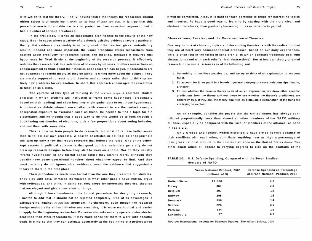
24 Chapter 2

with w h i c h to test the theory. F ina l ly , having tested the theory, the researcher should

either reject it or enshrine it solely on the basis of those new data. It is true that this

procedure erects formidable barriers to protect us from ex post facto argument, but it

has a number of serious drawbacks.

In the first place, it lends an exaggerated significance to the results of the new

study. E v e n in cases where a variety of previously existing evidence favors a particular

theory, that evidence presumably is to be ignored if the new test gives contradictory

results. Second and more important, the usual procedure deters researchers from

casting about creatively for research topics and theories. Because it requires that

hypotheses be fixed firmly at the beginning of the research process, it effectively

reduces the research task to a selection of obvious hypotheses. It offers researchers no

encouragement to think about their theories once research has begun. Researchers are

not supposed to remold theory as they go along, learning more about the subject. They

are merely supposed to react to old theories and concepts rather than to think up en­

tirely new problems for explanation. In short, this approach encourages the researcher

to function as a clerk.

T h e epitome of this type of thinking is the research design—a common student

exercise in wh ich students are instructed to frame some hypotheses (presumably

based on their reading) and show how they might gather data to test those hypotheses.

A doctoral candidate w h o m I once talked with seemed to me the perfect example

of repeated exposure to exercises such as these. He needed to find a topic for his

dissertation and he thought that a good way to do this would be to look through a

book laying out theories of elections, p ick a few propositions about voting behavior,

and test them with some data.

T h i s is how we train people to do research, but most of us have better sense

than to fol low our own precepts. A search of articles in pol i t ical sc ience journals

wi l l turn up only a few that report research that fo l lows the rules. O n e of the better-

kept secrets in pol i t ical sc ience is that good pol i t ical scientists general ly do not

draw up research designs before they start to work on a topic. Nor do they usual ly

"frame hypotheses" in any formal sense before they start to work, although they

usual ly have some operational hunches about what they expect to f ind. A n d they

most certainly do not ignore older ev idence, even the evidence that suggested a

theory to them in the first place.

The i r procedure is m u c h less formal than the one they prescribe for students.

They play with data, immerse themselves in what other people have written, argue

with col leagues, and think. In doing so, they grope for interesting theories, theories

that are elegant and give a new slant to things.

Al though I have condemned the formal procedure for designing research,

I hasten to add that it should not be rejected completely. One of its advantages is

safeguarding against ex post facto argument. Furthermore, even though the research

design undoubtedly stifles initiative and creativity, it is more methodical and easier

to apply for the beginning researcher. B e c a u s e students usual ly operate under stricter

deadlines than other researchers, it may make sense for them to work with specif ic

goals in mind so that they can estimate accurately at the beginning of a project when

Political Theories and Research Topics 25

TABLE 2-2 U.S. Defense Spending, Compared with the Seven Smallest

Members of N A T O

Gross National Product, 2005 (billions of $)

Defense Spending as Percentage of Gross National Product, 2005

United States 12,500 4.0

Turkey 363 3.2

Belgium 297 1.6

Norway 295 1.6

Denmark 258 1.4

Greece 226 3.0

Portugal 184 1.6

Luxembourg 37 0.7

Source: International Institute for Strategic Studies, The Military Balance, 2006.

it w i l l be completed. A l s o , it is hard to teach someone to grope for interesting topics

and theories. Perhaps a good w a y to learn is by starting with the more clear and

obvious procedures, then gradually loosening up as experience is gained.

O b s e r v a t i o n s , P u z z l e s , a n d the C o n s t r u c t i o n o f T h e o r i e s

One way to look at choosing topics and developing theories is with the realization that

they are at heart very commonsensica l processes, based on our daily experiences.

Th is is often lost in the forest of scholarship, in w h i c h scholars frequently deal with

abstractions (and with each other's rival abstractions). But at heart all theory-oriented

research in the social sciences is of the fol lowing sort:

1. Something in our lives puzzles us, and we try to think of an explanation to account

for it.

2. To account for it, we put it in a broader, general category of causal relationships (that is,

a theory).

3. To test whether the broader theory is valid as an explanation, we draw other specific

predictions from the theory and test these to see whether the theory's predictions are

generally true. If they are, the theory qualifies as a plausible explanation of the thing we

are trying to explain.

As an example , consider the puzz le that the Uni ted States has a lways con­

tributed proportionally more than almost al l other members of the N A T O mil i tary

al l iance, especia l ly as compared with the smal ler members of the al l iance, as seen

in Table 2 -2 .

O n l y G r e e c e and Turkey , w h i c h histor ical ly have armed heavi ly because of

their conf l ic ts wi th each other, contribute anything near as h igh a percentage of

their gross national product to the c o m m o n a l l iance as the Un i ted States does. T h e

other sma l l a l l ies all appear to vary ing degrees to ride on the coattails of the

26 Chapter 2

United States. One way to explain this would be to treat it as a specific instance of a more general relationship—that in any voluntary cooperative group the member with the greatest resources always tends to make disproportionate contributions. That is, a member who sees that the group would fail without her contribution will come through strongly; a relatively insignificant member will see that the group would do about equally well whether or not he contributes, and will tend to sit back and be a free rider. In the NATO example, if the United States does not contribute vigorously, the alliance languishes, but little Denmark hardly makes a difference one way or another.

A lot of the political scientist's creativity will then come into play in devising other, testable predictions from the theory to see whether it is generally valid. In this example we might examine chambers of commerce to see whether the biggest merchants in town usually carry most of the freight. Or we might look at trade union-supported political parties such as the Labour Party of Great Britain to see whether the largest unions carry a disproportionate share of the burden. If the theory holds up well across a variety of such tests, it will be a plausible potential explanation for the "Denmark problem."5

Lest working out a theory or a puzzle should seem too easy or too pat from these examples, let me review for you a puzzle currently in real play, to show the uncertainty and the progression of steps by which scientific discussion of a puzzle usually proceeds in real life.6 A great deal of attention has been directed over the past decade to the so-called democratic peace—the observation that no democracy has ever been observed to initiate war with another democracy. It is extremely rare in the social sciences for any relationship to be as invariant as this one, and the relationship is also of great importance in the assessment of democracy, so it is not surprising that this has attracted the attention of some very good minds.

First of all, a number of scholars have questioned whether the observation is as infallible as it is claimed to be. Both "democracy" and "war" are subject to a certain amount of interpretation. Since no country is a pure democracy, how much democracy is enough to have the country count as democratic? When the NATO alliance attacked the Yugoslavian government of Slobodan Milosevic in 1998 (a government which had been elected, but in an election without much real com­petition), was that a case of democracies attacking another democracy? Similarly, "war" is not always a black-and-white concept. When the U.S. Central Intelligence Agency gave covert support to a military coup against democratically elected President Allende of Chile, was that war?

The theory used in this example derives from the broader theoretical structure of Mancur Olson's The Logic of Collective Action (1965), which was discussed in pp. 6-7. The structure of argument discussed in this section—see a puzzle, frame an explanation based on a more general principle, devise other unrelated predictions from the general principle in order to test it—is presented skillfully by Charles A. Lave and James G. March in Introduction to Models in the Social Sciences (1975), especially in the first three chapters.

6 The discussion that follows draws heavily on the useful review of the democratic peace literature in Bueno de Mesquita et al. (1999).

Political Theories and Research Topics 27

Granting the gray areas of definition, however, most political scientists consider the democratic peace to be an enduring relationship of quite unusual regularity. This obser­vation, then, poses the puzzle: Why is it that democracies do not attack one another?

There have been two primary explanations offered. First, many scholars argue that democracies share a number of values in common, such as respect for individual liberties and a high value on competition. They also share an international norm of com­promise and bounded resolutions to conflicts. These characteristics, it is said, make democracies unlikely to wage war on those with whom they agree in so many areas.

Alternatively, a number of scholars point to the institutional structure of democracies as the explanation. People generally do not want to fight wars, and in democracies the wishes of the broad populace count for more than in nondemocra-cies. Accordingly, the chance that two democracies will enter a war, if in both of them the people's concerns count for a good deal, is low.

But beyond these two broad positions, as the diffuse scientific "conversation" has proceeded, many subtly nuanced theories have been developed. As one example, Bueno de Mesquita et al. (1999) point out that both of the broad explanations are hard to reconcile with the fairly strong willingness of democracies to initiate wars of conquest or empire. In the late nineteenth century, for instance, democratic France and Great Britain frequently sent armed forces to help acquire additions to their empires. And in the early twentieth century, the democratic United States enthusiastically engaged Spain in a war intended to lift some parts of the Spanish Empire such as Puerto Rico and the Philippines. These were not wars waged on democracies, but it was certainly the case that democratic values, and the influence of "the neople" in these democracies, did not prevent these countries from entering into warfare rather happily.

Bueno de Mesquita and his coauthors propose instead a slightly complicated explanation based on rational choice theory.

1. In a democracy, a leader must satisfy a fairly large number of people in order to stay in

power; in an autocracy, leaders typically need satisfy only a small number—the army,

for instance—or a single party.

2. A war involves costs, but also benefits if won. A democratic leader needs a higher ratio

of potential benefits to costs to justify going to war than an autocrat does, because the

democratic leader has to reward more people. (See [1.] above.) Therefore, the stakes are

higher for democratic leaders. An autocrat might lose a war yet stay in power (Saddam

Hussein of Iraq was an example, continuing in office after he lost the first Gulf War in

1991; he was ousted only later by direct action of American troops in 2003.) It is hard

to imagine a democratic leader losing a war and not being voted out of office.

3. Since the stakes are higher for democratic leaders, they will be more careful about

entering wars than will autocrats; and once involved in wars, democratic leaders will

fight them more determinedly.

4. Given reasonably good information about each other, it is unlikely that either of two

democrats involved in a conflict will think that he or she has a preponderant chance of

winning a war; and each will know that the other (because it is a democracy) will fight

very determinedly if there is a war. Therefore, the countries can be expected to try to

negotiate their disputes rather than go to war over them.

28 Chapter 2

This is a good explanation, but it certainly has not represented the last word in political scientists' collective effort to work out an explanation of the puzzle. (A good exercise for you would be to frame rebuttals of the rational choice explanation from the standpoint of the first two explanations—the "shared values" explanation and the "institutional role of the people" explanation.)

Note that throughout this discussion of puzzles and explanations. I have said that what is produced is a plausible potential explanation. It typically is the case that more than one plausible potential explanation can be produced for anything needing explanation. It then becomes the task of the scholar to decide among them on the basis of how broadly they apply, how simple they are (remember, a theory that is as complicated as the reality it is meant to explain has not gotten you very far), how accurately they predict, and so on. But the basic building blocks of political explanation are plausible potential explanations, derived in just the way that I have outlined here.

MACHIAVELLIAN GUIDE TO DEVELOPING RESEARCH TOPICS

There are really no guidelines that I can give you for developing a research topic other than to remind you once again that you are working toward results that are both new and elegant. Perhaps if we view the development task from the perspective of political research in general, however, we will gain some clue as to its place in the entire scheme.

Implicit in this chapter is the view that scholarly research represents a loose cooperative effort among many people. I mentioned earlier the pleasure that researchers feel in creating something that no one has seen before. This is mixed, however, with a sense of pride in being part of an ongoing tradition. One's work is something brand new, but it also draws on Karl Marx, or Emile Durkheim, or Robert Putnam, and modifies the meaning of their work. Scholars involved in devel­oping theory form a kind of priesthood—admittedly sometimes run less on faith and more according to the laws of laissez-faire and caveat emptor—focused on the common goal of perfecting elegant theories. As we have seen, the celebrants carry on this process by developing new theories and adapting old ones, fitting these theories to the real world to see how accurately they predict things, and feeding the results of such research back into the body of theory.7

From this description of the process of research, we can derive a set of rules to guide the individual researcher. If empirical research is motivated by a desire to affect the state of theories, either by confirming them or by working changes in

'Needless to say, it is not quite as neat as this. For one thing, a given person usually does not handle all these aspects of a particular problem. One person may work simply at clarifying theories, another may do a descriptive study of a partcular case, and a third may relate the new evidence to the body of older theory. Most researchers can expect to carry on any or all activities at any time.

Political Theories and Research Topics 29

them, you will be doing your best job when you maximize your effect on theory with a given investment of time and money. To do this, you must:

/. Maximize the generality of the theory you intend to examine. This is basically a restatement of the first criterion for elegant research. Note, though, that this rule is not something absolute, for any phenomenon can be examined at different levels of generality. One person may be hit on the head by an apple and form a theory of falling apples; another may have the same experience and form a theory of universal gravitation. The physical activity of the "study" is the same in both cases; the difference lies solely in the level at which the researcher works.

As an example from political science research, consider the variety of studies done on the presidency. The narrowest range of theory is found in biographies of particular presidents. The researcher in such a biography generally is concerned only with explaining what happened during a particular president's life, especially during his term in office. A broader range of theory is aimed at in studies of the U.S. presidency, which may analyze the nature of the office, the sources of executive power, the way in which presidents' personalities can influence their behavior in office, and so on.8 A still broader range of theory is seen in studies that use the U.S. presidency as an example of sovereigns in general and seek to explain the sources and limitations of sovereign power. Richard Neustadt's Presidential Power and the Modern Presidents (1991), for instance, often operates at this level of generality.

2. Pick a weak theory to work on. The weaker the previous confirmations of a theory have been, the greater your contribution will be. Of course, you have a greater probability of refuting a weak theory. But also, if your research does confirm the theory, your work will again be more significant than if the theory already had a good deal of confirming evidence.

Perhaps the best way to use the strategy of picking a weak theory is to state a new, original theory yourself. In this case, your hypotheses are necessarily in need of proof, and any evidence you can buttress them with will be important. Remember, though, that "new, original theories" that are also elegant are hard to come up with.

Another way to follow this strategy is to pick an anomaly—that is, a question on which previous research has been contradictory. A good example of research stimulated by an anomaly is the study by Sidney Tarrow (1971) of the political participation of French peasants. Tarrow was struck by the fact that although French peasants regularly responded to surveys by stating that they were not very interested in politics, they also regularly turned out to vote in greater numbers than did the urban French.

This anomaly led Tarrow to probe more deeply into what political involvement means to the French, so as to resolve the apparent contradiction. His conclusions led to the rejection of the traditional "interest in politics" measure. They also shed new light on

8 For example, a study of the nature of the presidential office (such as Koenig, 1968), a study of presidents' political personalities (Barber, 1972), or an analysis of presidents' leadership (Greenstein, 2000).

30 Chapter 2

the nature of French voters' attachment to political parties. On this hinged the apparent

contradiction, since French peasants were fiercely independent and understood "interest

in politics" to imply some sort of approval of the existing parties. Though they were in

fact interested in politics, they denied this because of their antipathy to the parties.

Anomal ies such as this are hard to come by, because earlier investigators generally have

noticed them already and have tried to resolve them. If you can find an anomaly having

to do with a significant area of political theory, however, you can be certain that any

plausible efforts at resolution wil l be interesting.

Another example of a nice anomaly just waiting to be analyzed is the fact that

in the 2000 elect ion, the higher voters' incomes were, the more l ikely they were to

vote for George W. B u s h . B u t if you look at the "red states"—the states he c a r r i e d —

they are on the whole poor states with low average incomes. What sort of theory

might you devise to explain this?

Besides anomalies, you might choose a problem you believe has just not been

sufficiently researched, perhaps one in which all variables have not been covered. Thus ,

you might replicate a study in a different context from the original one. Arthur A.

Goldsmith (1987) noted that Mancur Olson's (1982) wel l -known theory, that prolonged

political stability produces rigid social and economic structures that retard economic

growth, was based mostly on the experiences of the West and Japan. T h e Third World

would provide a laboratory of less-developed countries with a wider range of cultures

and economic circumstances. In fact, Goldsmith found that examination of these coun­

tries did not support Olson 's theory, though he hastened to add that his measure of

"instability" was questionable and might have been a source of the disparity. T h e most

likely reason, at least to my taste, is that the context is different. Olson's theory relies on

the negative economic effects of organized interest groups. Such groups are strong and

active in the countries Olson studied, but not in the Third World context that Goldsmith

studied. Goldsmith's negative results may thus point up the importance of organized

interest groups in Olson 's theory.

3. Make the connection between the general theory and your specific operations as clear as possible. T h i s really just boils down to making sure you say what you

think you are saying. It involves such things as the accuracy of your deductions from

the theory to the specif ic situation, the accuracy with w h i c h you have measured

things, and so on. M u c h of the rest of this book focuses on such problems.

Y o u may have noticed that these three rules resemble the criteria for elegance

fairly closely. Y o u also may have noticed that the basic phi losophy behind t h e m —

" D o research that makes as big a splash as poss ib le"—reads l ike a guide for ruthless

and hungry assistant professors. But each of the rules, derived from my underlying

Machiave l l ian outlook, also has a beneficial effect on the field as a whole. If indiv id­

uals choose those problems of theory that have so far had the weakest verif ication,

for example, the entire field wi l l benefit from an examination of those theories most

in need of investigation.

Needless to say, these guidelines should remain flexible enough to allow

different mixes of research strategy. There is no one "scientif ic method" involved here.

Political Theories and Research Topics 31

One person may find a tool that measures a variable better than had been done before

and then simply apply it to sharpen previously examined relationships. Another may

note an anomaly in a theory and organize an experiment to resolve the problem. A third

may look over previous research findings and place a new, broader, or simpler inter­

pretation on them. A l l are following the rule of maximizing their impact on theory.

4. Present your theory as clearly and vividly as possible. A Machiave l l ian

researcher wants to inf luence as many people as possible, so it makes sense to make

your reader's life easier and your message more compel l ing. T h i s means, write we l l

and present any graphic information we l l . People often think how you say something

is separable from what you say, but that is s imply not true. I f the purpose of theory

is to change people's understanding of the world, then the way the theory is c o m m u ­

nicated to them is an integral part of the development of the theory.

H o w to write wel l and design graphic displays we l l are beyond the scope of

this book; each really requires a book in its own right. Fortunately, I can suggest two

truly good books that w i l l help you. For writ ing, I recommend Wi l l i am Knowl ton

Z insser 's On Writing Well: The Classic Guide to Writing Nonfiction (New York:

HarperCol l ins , 1998). An excellent introduction to good graphic presentation

is E d w a r d R. Tufte 's The Visual Display of Quantitative Information (Cheshi re ,

C o n n . : Graph ics Press , 1983).

F U R T H E R D I S C U S S I O N

A n intriguing book relevant to this chapter is Arthur Koest ler 's The Act of Creation (1969). An article that presents some interesting, rather controversial ideas about

appropriate ways to build and test theory is Rona ld Brunner 's "An ' Intentional '

Alternative in Publ ic Opin ion R e s e a r c h " (1977) . Another perspective is offered

persuasively by J . Dona ld Moon (1975) . An excellent introduction to building

elegant theories is found in the f irst three chapters of L a v e and M a r c h (1975) . S o m e

questions you might consider are:

1. Presumably, work in normative philosophy or in formal theory could be evaluated in

terms of elegance, just as empirical research is. What changes would this require in the

definition of elegance?

2. This chapter has implied that the usual way to come up with a theory is to focus on a

body of observations and look for regular patterns in them. Although this is the usual

procedure, it is neither the only nor necessarily the best approach. What drawbacks

might it involve? In what alternative ways might one develop a theory?

3. I stated in this chapter that most social science theories are causal. What would a

noncausal theory look like? Under what circumstances would it be likely to be used?

{Hint: Consider Einstein's famous theory, E = mc .)

Chapter 3

m mkM

In Chapte r 2, I argued that f lexibi l i ty and o r i g i n a l i t y — i n a word , f r e e d o m — a r e

important in doing good research . In this chapter I sha l l stress the need to state

theories in a c lear , unambiguous w a y — a form of se l f -d isc ip l ine that must a c c o m ­

pany such f reedom.

In particular, we shall be concerned with framing theories in terms of concepts

that cannot easily be subdivided into further distinct meanings, either denotative or

connotative—in other words, very simple concepts whose meaning is unequivocal.

I shall cal l such simple concepts unidimensional, in contrast to concepts whose meaning

may vary from reader to reader and even from time to time, that is, multidimensional

concepts.

Consider the fol lowing example: As a description of cl imates, "temperature" is

a unidimensional concept. Temperature can vary along only one dimension, from hot

to cold. Therefore, if a theory states that a temperature below x degrees causes the

spotted ibex to stop breeding, that statement wi l l mean the same thing to every reader.

" G o o d weather," on the other hand, is a mult idimensional concept that involves

among other things temperature, wind velocity, humidity, amount of precipitation,

and degree of cloud cover. If there is a variation along any one of these separate

dimensions, the "goodness" of weather varies. If the theory stated that "bad weather"

caused the spotted ibex to stop breeding, the meaning of that theory would be left to

the reader's judgment. Is it rain that discourages the ibex's ardor? Or do high winds

make h im think of other things? Is it the heat? T h e humidi ty?

As we can see from this example, it is preferable to frame theor ies in terms of

unidimensional rather than multidimensional concepts. T h e Eng l ish language does not

always make this easy, however. In this chapter we shall look at the Eng l ish language

in general and at the varied theories that may be hidden in ordinary language.

32

Importance of Dimensional Thinking 33

E N G L I S H A S A L A N G U A G E F O R R E S E A R C H

I have assumed so far that if pol i t ical research is to be useful , a min imal requirement

is that its results should mean the same thing to any two different readers.

Unfortunately, the E n g l i s h language is badly designed to function as a medium for

stating research results clearly and without ambiguity. Most E n g l i s h words can take

on a variety of meanings, depending on the context and on the mood of the reader. To

use an everyday example, the statement, " T h e welfare bi l l failed in the House

because the administration did not fight for it," might mean:

1. A welfare bill w a s passed , but no t the one the wri ter wanted .

2. No welfare bill passed at all.

Whichever of these is the case , the failure could have resulted from any number of

other events, for example:

3. T h e adminis t ra t ion pr ivately pas sed the word to its suppor te r s to undercu t the bill .

4 . T h e adminis t ra t ion wan ted the bil l , but did not c a m p a i g n as hard as i t usual ly does for

bi l ls it wan t s .

5. T h e adminis t ra t ion c a m p a i g n e d as hard as i t usual ly does for bills i t wan t s , but not as

hard as the wri ter w o u l d have d o n e .

6. T h e adminis t ra t ion w e n t al l -out for the bill , but failed to get i t p a s s e d — a n d the wr i te r is

in the oppos ing party.

Note that in these statements there are many additional phrases that are ambiguous:

"pass the word," "undercut the bill," "want the bill," "campaign for the bill," "go all-out."

As another example of a mult idimensional concept, consider political party.

T h i s concept can be broken down into at least six component dimensions: those

people who vote for the party in a given election, those people who are registered

with the party, those people who identify themselves in their minds with the party,

those people who do voluntary work for the party at some given time, the officers of

the party, and those who are running or elected as candidates under the party label.

W h e n researchers write about "the polit ical party," they may be referring to any or al l

of these various dimensions of the term. T h u s , unless polit ical scientists specify

which dimensions apply, they may merely succeed in creating confusion. A few

further examples of mult idimensional terms are: power, enjoyment, conservative,

economic development, intelligent, and love.

Debates in political science sometimes resolve themselves into the fact that

participants are using the same term in different ways. The word liberal, for instance, has

many dimensions, some of which are probably even inconsistent. Just to look at one of its

dimensions, it often connotes "free-spending," although in its original usage, which is

still fairly current in Europe, it means "favoring a limited role for government." Since

liberal has generally unpopular connotations in the United States and is multidimension­

al in complex ways, it is natural to use this flexible word as a club in describing candi­

dates. In the election of 1996, for instance, the late Senator Paul Wellstone of Minnesota

34 Chapter 3

was described by his opponent as "embarrassingly liberal" for his vote against a bill re­

ducing welfare payments. He responded that his vote was actually "deeply conservative"

because it reflected the moral values of Minnesotans. Was Wellstone's vote "liberal" or

"conservative"? The argument proceeded almost irrespective of its merits.

T h e strategy I am introducing here, framing theories in terms of unidimensional

concepts, can help us to keep clear the meanings of the words we use and to avoid this

kind of confusion.

Ordinary Language

As we have just seen, many Eng l i sh words involve more than one dimension, and these

component dimensions are rarely specified in ordinary language. Mult idimensional

concepts are valuable and useful in ordinary language, as is indicated by their popular­

ity. T h e connotations accruing to a word that means many different things simultane­

ously add richness to our language. Art and rhetoric could not be restricted to

unidimensional vocabularies.

But in the social sciences, we pay a high price for this benefit. R i c h connotations,

which are so important to art, get in the way of analytic thinking. A poet is pleased if she

chooses a word whose meanings give the reader pause for thought; it is the poet's job to

create a rich confusion of varied nuances. The job of the social analyst, however, is to

bring order out of social chaos by means of simple theories.

Mul t id imensional words hamper socia l scientists in at least three ways:

1. Poor communication. Because a reader can never be certain what meaning an author

intended, multidimensional words in effect hamper communication.

2. Difficulty with measurement. Whenever social scientists want to measure a variable,

they confront an impossible task unless they have defined the variable in such a way

that it consists of a single dimension. For example, consider a political scientist

who wanted to measure the "amount of interaction" between various nations. Now,

"interaction" involves a number of dimensions: alliances, volume of trade, tourism,

exchanges of mail, and so on. Suppose that this political scientist discovered the

following things about countries A, B, and C:

Between Volume Items of Countries Trade/Year Mail /Year All iance

A and B $10 billion 20 million Yes

B and C $5 billion 30 million Yes

A and C $20 billion 10 million No

Between which two countries is there greater interaction? A and C trade together a great

deal but are not allies; B and C exchange a great deal of mail but do not trade together as

much as A and B. Clearly, "amount of interaction" is not a unidimensional variable. Had

the investigator chosen three separate measures—trade, mail flow, and alliance—there

would have been no problem in comparing the countries. We can confidently state, for

instance, that A and C share the greatest trade, followed by A and B and by B and C. We

return to such problems of measurement in Chapter 4.

Importance of Dimensional ininmng ->3

'Today, of course, reality has caught up with rhetoric in the explosive economic growth of countries such as China, India, and South Korea.

3. Ambiguous associations. From the standpoint of the social scientist, another fault in

multidimensional words is that each such word is itself a theory of sorts. By associating

several distinct things with a single term, a multidimensional word implies the theory

that these things go together. But unless its component dimensions are made explicit, it

is a poorly articulated and poorly controlled theory. For example, the word wise has long connoted (1) broad practical knowledge,

(2) a highly developed understanding of relationships, (3) a contemplative bent, and

(4) a background of long practical experience. Among other things, it has implied the

theory that the older (and thus the more experienced) one got, the better one understood

things. So, if I use the word wise rather than intelligent, my reader picks up this little

theory subliminally embedded in my statement.

T h e o r i e s such as this, embedded in mul t id imens iona l words , change as

c o m m o n usage ref lects changed moods and new exper iences . B u t the process by

w h i c h they change is not a very sat isfactory one; it is a process that g ives us little

conf idence in the new theories that are produced. It may be an unart iculated

d is l ike for the theory impl ied by the w o r d wise, for example , w h i c h has led to

d imin ished use of the word in egal i tar ian A m e r i c a , and its degradation in s u c h

slang as " D o n ' t get w i s e wi th m e ! " and " w i s e guy." I t is in jus t s u c h a w a y that

word usage gradual ly changes , ref lect ing different v i e w s of the wor ld . T h e polite

substitution of the term developing nations for underdeveloped countries in the

1950s and 1960s is another example . T h i s change in usage ref lected the changed

status of the T h i r d Wor ld and at least some hopeful th inking about what w a s

happening there. 1

T h i s process of theory development is uncontrol led. In a sense it is very

democra t ic—probab ly more democrat ic than we w o u l d l ike. E v e r y o n e w h o uses a

part icular word takes part in the process , and a person 's inf luence is more or less

proportional to the number of people w h o hear her use the word . T h e r e is no pro­

v is ion made for greater inf luence on the process by those w h o know more about

the subject . D ic t ionar ies , by codi fy ing word usage, serve to s low down the process

of change, but they do not affect the quality of the change.

Another prob lem wi th the process is that these changes often proceed at a

sna i l ' s pace . T h u s , theories that are embedded in mul t id imens iona l words surv ive

pract ical refutation m u c h longer than i f they were made expl ic i t . T h e words

liberal and conservative are a case in point. B e c a u s e s u c h attitudes as a desire for

e c o n o m i c a c t i v i s m on the part of government , concern for the legal rights of ind i ­

v idua ls , p a c i f i s m , and internat ional ism often seemed to go together w h e n one

looked at the pol i t ica l elite in the Un i ted States, the term liberal c a m e to denote

their presence and conservative their absence. ( T h e words were borrowed f rom a

E u r o p e a n context, but their meanings were cons iderab ly changed , w h i c h only

added to the subsequent confus ion . ) T h e impl ied theory—that these attitudes

tended to c o i n c i d e — w a s never very accurate as a descr ipt ion even of the elite and

36 Chapter 3

i t has proved to be quite inaccurate in descr ib ing people in genera l . I t turns out,

for example , that people w h o are l iberal on ind iv idua ls ' r ights are often c o n s e r v a ­

tive on e c o n o m i c i ssues . A l l this went unnot iced unti l at least the late 1940s, so

that even today there are sti l l many people w h o use the words liberal and

conservative in this way, as if they had general va l id i ty . 2

T h u s , whi le changes in usage do produce changes in the theories implied by

mult idimensional words, the process by which these changes are made is capr ic ious;

this is presumably not the way we want to develop socia l theory. Soc ia l scientists

should be uncomfortable if hidden away in their statement of a theory are additional

little theories that are implicit and uncontrolled.

L e t me sum up the argument thus far: Socia l scientists should use unidimen­

sional language for three reasons:

1. T h e mean ing of a theory is not unambiguous ly clear if it is couched in mul t id imensional words .

2. Variables canno t be measu red u n a m b i g u o u s l y if they have been def ined in a mul t id i ­

mens iona l way.

3. Inclus ion of mul t id imens iona l words in a theory confuses that theory wi th addi t ional

theor ies that are impl ied by the exis tence of the mul t id imens iona l words themse lves .

Despite our prescription, however, we must acknowledge the fact that the E n g l i s h

language contains many words that hold a r ich variety of meanings and

connotations. These are to be valued in their own right, yet social scientists often

must create their own vocabulary. I f ordinary language does not provide unidimen­

sional words for the things socia l scientists want to say, they must invent the words

themselves. T h i s is one reason that social sc ience writ ing so often strikes readers as

flat and co ld . What most people mean by "soc ia l sc ience j a rgon" is the unid imen­

sional vocabulary invented by social scientists for their use in analytic research.

Wri t ing from w h i c h the r ichness of varied connotations has been removed is

flat. T h i s is s imply one of the costs we must pay to write analytically. Of course, this

is not meant to excuse poor writ ing in the social sc iences or anywhere else.

Unid imensiona l language is a minor handicap under wh ich socia l scientists operate,

but it need not prevent them from writ ing clear and graceful prose.

Actually, writers in any analytic field suffer the same handicap. Natural scientists

must create their own vocabularies, too. But somehow the loss of richness seems more

painful in the social sciences than in other fields. T h e physicist may describe a body's

motion in terms of "mass," "velocity," and "acceleration" rather than saying that it

"Another example of meanings of words being slow to change, an amusing one, is offered by the old saying "the exception that proves the rule." Taken at face value—as it usually is—this phrase is idiotic. An exception does not prove a rule, but should cause us to reconsider the rule. The secret is that centuries ago to "prove" meant to submit to a test; in fact, the word has the same root as "prove," and was used in phrases such as "submit to a proof by fire." The phrase about exceptions has continued, with " p r o o f included in it, even though the changed meaning of the word has rendered the phrase meaningless.

Importance of Dimensional Thinking 37

"hurtles through space," and the mind does not rebel. But when the political scientist

describes politics as consisting of "system inputs," "system outputs," and "feedback

loops," the mind does rebel. Th is is because the social scientist deals with people, the

thing we care most passionately about. It does not bother us when a physicist tries to

reduce the complex motion of a particle to unidimensional concepts, but when social

scientists try to simplify the complex reality of politics, the family, or of protests, we are

disturbed.

P R O P E R U S E O F M U L T I D I M E N S I O N A L W O R D S

I have argued that we should try to use only indiv is ib le d imens ions as concepts in

pol i t ical sc ience . B u t there is another side to the quest ion, w h i c h leads me to

temper that stance somewhat . A l though it is a lways necessary to think and work

with un id imensional concepts in the socia l sc iences , it may be convenient to put

separate d imens ions together in explicit mul t id imensional combinat ions.

"National integration" may provide an example of such a concept. There are

many d imensions impl ied in the term: political consensus within the nation; wide­

spread communicat ion and personal interchanges within the nation; a feel ing, among

the nation's people, that they all belong together; legal integration; and so on. It

would be possible to do without the term national integration, and work directly

with these dimensions, but it would be awkward . There are a great number of

dimensions involved, and they may combine in odd ways . At the same time, there is

a widespread feeling among political scientists that these things tend to go together

to constitute a general process. T h i s process might not be at al l easy to discern if we

were forced to work simultaneously with the large number of unidimensional c o n ­

cepts involved in it. Accord ing ly , polit ical scientists over the last few decades have

explicit ly developed the term national integration, composed of these various

d imensions, to refer to the general process. T h e result has not been fully satisfactory,

but there does appear to be a need for such a summary term.

T h e use of an explicit combination of separate d imensions such as this has

some of the advantages of both "ordinary language" and unidimensional language,

and some of the disadvantages of each. S u c h summary constructs may add grace and

interest to the presentation of your results and ideas. T h e y may add clarity, too, if

you are work ing with so many dimensions simultaneously that readers would have

difficulty keeping track of them. A n d they help to keep your theory parsimonious.

S u c h explicit combinations of dimensions have the advantage, as compared

with ordinary language, that you have built your own juxtaposit ion of d imensions

into the word. However , these contrived concepts retain many of the disadvantages

of ordinary language. A reader cannot tell, for example , when faced with a high

score on a variable that combines dimensions A, B, and C, whether this means that A

and B were high and C low, or that B was high and A and C were low, or whatever.

Al though explicit mult idimensional words are more useful than ordinary language,

you should not use them casual ly .

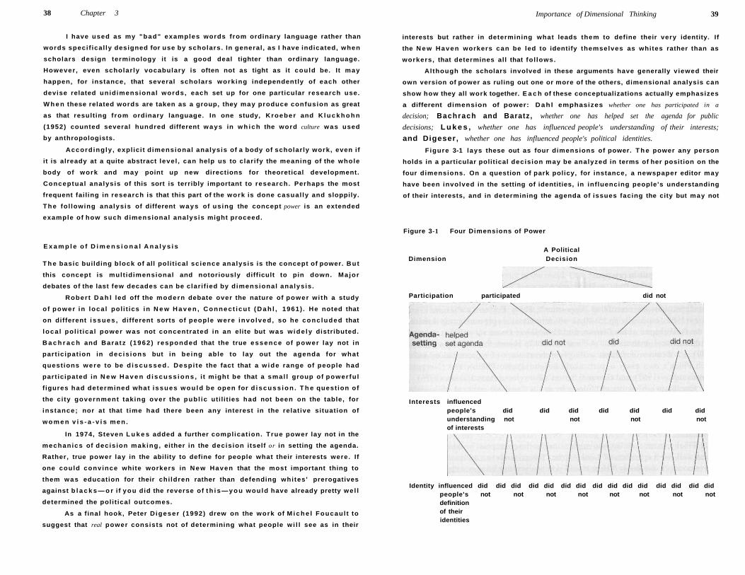
38 Chapter 3

I have used as my "bad" examples words from ordinary language rather than

words specif ical ly designed for use by scholars. In general , as I have indicated, when

scholars design terminology it is a good deal tighter than ordinary language.

However , even scholar ly vocabulary is often not as tight as it could be. It may

happen, for instance, that several scholars work ing independently of each other

devise related unidimensional words, each set up for one particular research use.

W h e n these related words are taken as a group, they may produce confusion as great

as that resulting f rom ordinary language. In one study, Kroeber and K l u c k h o h n

(1952) counted several hundred different ways in w h i c h the word culture was used

by anthropologists.

Accord ing ly , expl ici t d imensional analysis of a body of scholar ly work, even if

it is already at a quite abstract level , can help us to clar i fy the meaning of the whole

body of work and may point up new directions for theoretical development.

Conceptual analysis of this sort is terribly important to research. Perhaps the most

frequent fai l ing in research is that this part of the work is done casual ly and sloppily.

T h e fol lowing analysis of different ways of using the concept power is an extended

example of how such dimensional analysis might proceed.

E x a m p l e o f D i m e n s i o n a l A n a l y s i s

T h e basic building block of all poli t ical sc ience analysis is the concept of power. B u t

this concept is mult idimensional and notoriously difficult to pin down. Ma jor

debates of the last few decades can be clar i f ied by dimensional analysis .

Rober t D a h l led off the modern debate over the nature of power wi th a study

of power in loca l pol i t ics in N e w H a v e n , Connec t icu t ( D a h l , 1961) . He noted that

on different i s s u e s , different sorts of people were invo lved , so he conc luded that

loca l pol i t ica l power was not concentrated in an elite but was w i d e l y distributed.

B a c h r a c h and Bara tz (1962 ) responded that the true essence of power lay not in

part ic ipat ion in dec is ions but in be ing able to lay out the agenda for what

quest ions were to be d i s c u s s e d . Desp i te the fact that a w ide range of people had

part icipated in N e w H a v e n d i s c u s s i o n s , i t might be that a smal l group of power fu l

f igures had determined what issues w o u l d be open for d i s c u s s i o n . T h e quest ion of

the ci ty government taking over the publ ic uti l i t ies had not been on the table, for

instance; nor at that t ime had there been any interest in the relat ive situation of

w o m e n v i s - a - v i s men .

In 1974, Steven L u k e s added a further compl icat ion. True power lay not in the

mechanics of decis ion making, either in the decis ion itself or in setting the agenda.

Rather, true power lay in the ability to define for people what their interests were. If

one could convince white workers in N e w Haven that the most important thing to

them was education for their chi ldren rather than defending whi tes ' prerogatives

against b l a c k s — o r i f you did the reverse of t h i s — y o u would have already pretty we l l

determined the pol i t ical outcomes.

As a f inal hook, Peter D igeser (1992) drew on the work of M i c h e l Foucaul t to

suggest that real power consists not of determining what people w i l l see as in their

Importance of Dimensional Thinking 39

interests but rather in determining what leads them to define their very identity. If

the N e w Haven workers can be led to identify themselves as whites rather than as

workers, that determines all that fo l lows.

Although the scholars involved in these arguments have generally v iewed their

own version of power as ruling out one or more of the others, dimensional analysis can

show how they all work together. E a c h of these conceptualizations actually emphasizes

a different dimension of power: Dah l emphasizes whether one has participated in a

decision; Bachrach and Baratz, whether one has helped set the agenda for public

decisions; L u k e s , whether one has influenced people's understanding of their interests;

and Digeser, whether one has influenced people's political identities.

Figure 3-1 lays these out as four dimensions of power. T h e power any person

holds in a particular polit ical decision may be analyzed in terms of her position on the

four dimensions. On a question of park policy, for instance, a newspaper editor may

have been involved in the setting of identities, in inf luencing people's understanding

of their interests, and in determining the agenda of issues facing the city but may not

Figure 3-1 Four Dimensions of Power

A Political Dimension Decision

Participation participated did not

Interests influenced people's did did did did did did did understanding not not not not of interests

Identity influenced did did did did did did did did did did did did did did did people's not not not not not not not not definition of their identities

40 Chapter 3

have been involved in the actual decisions. A member of the city park board may have

been involved in the decision but may not have exercised power in any of its other

dimensions. An elementary school teacher may have been involved in the process of

forming identities but may not have exercised power in its other dimensions; another

school teacher, interested and active on park questions, may have been involved in the

process of forming identities, and may have participated in the decisions, but not have

exercised power in the other two dimensions.

D imens iona l analys is of this sort a l lows us to see the interrelations of various

approaches to a question and can also give us a r ich f ramework with w h i c h to apply

a mult id imensional concept. It also a l lows us to compare the importance of the

d imensions. Impl ic i t in each later scholar in the d iscuss ion sketched above was the

idea that his notion of power was deeper and more basic than those that went

before. A d imensional analys is gives us a structure within w h i c h we can address

this question.

F U R T H E R D I S C U S S I O N

F o r m a l treatment of d imensional analys is was introduced by A l l a n H. Bar ton , " T h e

Concept o f Proper ty -Space in S o c i a l R e s e a r c h " (1955) . Phi l ip E . Jacob 's "A Mul t i ­

d imensional C lass i f ica t ion of Atroci ty Stor ies" (1955) furnishes a good example of

d imensional analys is in practice.

Some examples f rom polit ical science are Chapter 11 of Robert D a h l ' s

Political Oppositions in Western Democracies (1966) , a first-rate analysis of the rel ­

evant d imensions for c lass i fy ing "opposit ion"; Harry E c k s t e i n ' s Pressure Group

Politics (1960) , especial ly pp. 1 5 - 4 0 , in w h i c h he classi f ies pressure group activities;

and the third chapter of his Division and Cohesion in Democracy (1966) , an exce l ­

lent dimensional analysis of "pol i t ical d iv is ion"; H a n n a Pitkin 's Representation

(1969) , a col lect ion of various writ ings on the concept of representation, among

w h i c h Pi tk in 's own essay is particularly insightful; also Pi tk in 's The Concept of

Representation (1967) ; and G iovann i Sartori 's Parties and Party Systems (1976) .

O n e b r a n c h of po l i t ica l ph i losophy is the "ana ly t ic po l i t ica l p h i l o s o p h y "

approach , w h i c h seeks to study pol i t ica l ideas by a c l o s e examinat ion of the

mean ing of concepts used to descr ibe po l i t ics . T h i s approach is r e v i e w e d in

R i c h a r d B e r n s t e i n ' s Restructuring of Social and Political Theory ( 1 9 7 8 ) and in

O p p e n h e i m (1975 ) .

F ina l l y , as an exerc ise , you might consider the conceptual problems involved

in the w e l l - w o r n aphor ism of L o r d A c t o n : " P o w e r tends to corrupt and absolute

power corrupts absolutely." H o w w o u l d you ana lyze this conceptua l ly? Can i t be

a n a l y z e d ?

Chapter 4

WClLTTTOClLTl]

Accuracy

In this chapter I explore problems of accurate measurement. T h e s e are problems

that arise when we try to relate the actual operations in a p iece of research—that i s ,

measures of th ings—to the concepts that form the basis of our under ly ing theory.

Concepts , of course, exist only in the mind. O n e necessary assumption, i f we are to

c la im that a piece of research has tested a given theory, is that the things measured

in the research correspond to the things in the theorist's mind.

T h i s is often a difficult assumption to make. In the preceding chapter, you saw

one k ind of problem that can stand in the way of it. T h e pol i t ical scientist w h o

wanted to measure the amount of interaction between nations found that there was

no single satisfactory indicator of "interaction." A number of th ings—trade, mai l

exchanges, a l l iance, and so on—par took of "interaction," but no one of them alone

was synonymous with the mental construct.

In the social sciences, only rarely are we able to measure our concepts directly.

Consider, for example, the concepts "socia l c lass," "respect for the presidency," and

"power in the community." A n y variables we would choose to measure these concepts

correspond only indirectly or in part to our mental constructs. T h i s is the basic problem

of measurement in the social sciences.

Cons ider the concept "soc ia l status." A m o n g social scientists there are two

popular versions of this concept: "subjective social status," the c lass that individuals

consider themselves as belonging to; and "objective socia l status," an individual 's

rank with regard to prestige along socia l hierarchies such as education, income, and

occupation. Neither version of the concept can be measured directly.

In the case of "subject ive soc ia l status," we cannot measure direct ly what

ind iv iduals feel about their status. We know what they report, but their repl ies to

our inquir ies may not be what we are look ing for. T h e y may not k n o w what they

" rea l l y" fee l , for instance; or they m a y misunderstand the question and give a

41

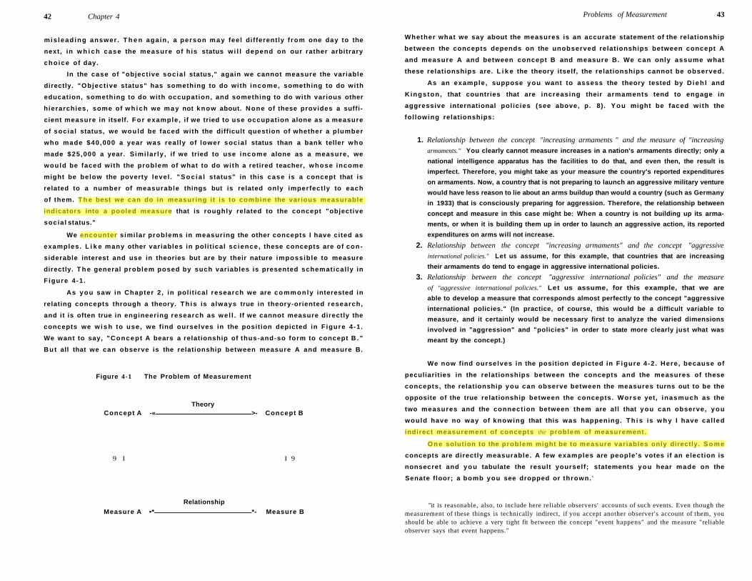
42 Chapter 4

mis lead ing answer . T h e n again , a person m a y feel differently f rom one day to the

next, in w h i c h case the measure of his status w i l l depend on our rather arbitrary

cho ice of day.

In the case of "objective socia l status," again we cannot measure the variable

directly. "Object ive status" has something to do with income, something to do with

education, something to do with occupation, and something to do with various other

hierarchies, some of w h i c h we may not know about. None of these provides a suffi­

cient measure in itself. F o r example, if we tried to use occupation alone as a measure

of socia l status, we would be faced with the difficult question of whether a plumber

who made $40,000 a year was real ly of lower socia l status than a bank teller who

made $25,000 a year. S imi lar ly , if we tried to use income alone as a measure, we

would be faced with the problem of what to do wi th a retired teacher, whose income

might be below the poverty level . " S o c i a l status" in this case is a concept that is

related to a number of measurable things but is related only imperfectly to each

of them. T h e best we can do in measuring it is to combine the various measurable

indicators into a pooled measure that is roughly related to the concept "objective

socia l status."

We encounter similar problems in measuring the other concepts I have cited as

examples. L i k e many other variables in poli t ical sc ience, these concepts are of con­

siderable interest and use in theories but are by their nature impossible to measure

directly. T h e general problem posed by such variables is presented schematical ly in

F igure 4 -1 .

As you saw in Chapter 2 , in poli t ical research we are commonly interested in

relating concepts through a theory. T h i s is a lways true in theory-oriented research,

and it is often true in engineering research as we l l . If we cannot measure directly the

concepts we w i s h to use, we find ourselves in the position depicted in F igure 4-1 .

We want to say, "Concept A bears a relationship of thus-and-so form to concept B . "

B u t all that we can observe is the relationship between measure A and measure B.

Figure 4-1 The Problem of Measurement

Theory Concept A -« >- Concept B

9 I I 9

Relationship

Measure A •* *- Measure B

Problems of Measurement 43

Whether what we say about the measures is an accurate statement of the relationship

between the concepts depends on the unobserved relationships between concept A

and measure A and between concept B and measure B. We can only assume what

these relationships are. L i k e the theory itself, the relationships cannot be observed.

As an example, suppose you want to assess the theory tested by D i e h l and

K ingston , that countries that are increasing their armaments tend to engage in

aggressive international pol icies (see above, p. 8). Y o u might be faced wi th the

fol lowing relationships:

1. Relationship between the concept "increasing armaments " and the measure of "increasing

armaments." You clearly cannot measure increases in a nation's armaments directly; only a

national intelligence apparatus has the facilities to do that, and even then, the result is

imperfect. Therefore, you might take as your measure the country's reported expenditures

on armaments. Now, a country that is not preparing to launch an aggressive military venture

would have less reason to lie about an arms buildup than would a country (such as Germany

in 1933) that is consciously preparing for aggression. Therefore, the relationship between

concept and measure in this case might be: When a country is not building up its arma­

ments, or when it is building them up in order to launch an aggressive action, its reported

expenditures on arms will not increase.

2. Relationship between the concept "increasing armaments" and the concept "aggressive

international policies." Let us assume, for this example, that countries that are increasing

their armaments do tend to engage in aggressive international policies.

3. Relationship between the concept "aggressive international policies" and the measure

of "aggressive international policies." Let us assume, for this example, that we are

able to develop a measure that corresponds almost perfectly to the concept "aggressive

international policies." (In practice, of course, this would be a difficult variable to

measure, and it certainly would be necessary first to analyze the varied dimensions

involved in "aggression" and "policies" in order to state more clearly just what was

meant by the concept.)

We now find ourselves in the position depicted in F igure 4-2 . Here , because of

peculiarit ies in the relationships between the concepts and the measures of these

concepts, the relationship you can observe between the measures turns out to be the

opposite of the true relationship between the concepts. Worse yet, inasmuch as the

two measures and the connection between them are al l that you can observe, you

would have no way of knowing that this was happening. T h i s is w h y I have cal led

indirect measurement of concepts the problem of measurement.

O n e solution to the problem might be to measure variables only directly. S o m e

concepts are directly measurable. A few examples are people's votes if an election is

nonsecret and you tabulate the result yourself; statements you hear made on the

Senate floor; a bomb you see dropped or thrown. 1

"it is reasonable, also, to include here reliable observers' accounts of such events. Even though the measurement of these things is technically indirect, if you accept another observer's account of them, you should be able to achieve a very tight fit between the concept "event happens" and the measure "reliable observer says that event happens."

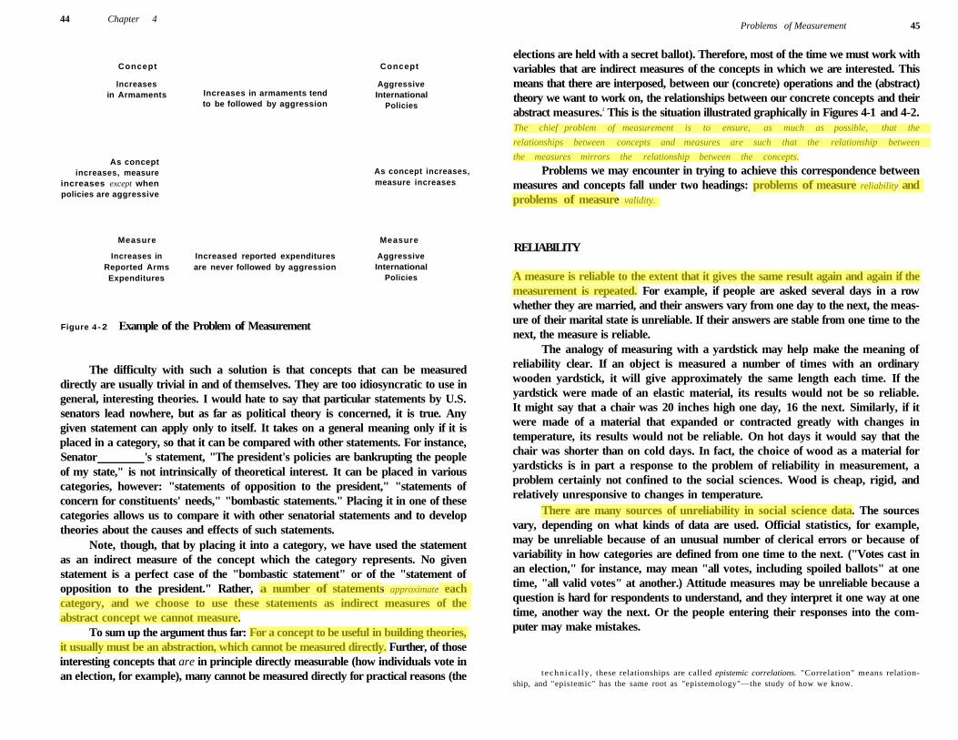
44 Chapter 4

Concept Concept

Increases in Armaments Increases in armaments tend

to be followed by aggression

Aggressive International

Policies

As concept increases, measure

increases except when policies are aggressive

As concept increases, measure increases

Measure

Increases in Reported Arms Expenditures

Increased reported expenditures are never followed by aggression

Measure

Aggressive International

Policies

Figure 4 -2 Example of the Problem of Measurement

The difficulty with such a solution is that concepts that can be measured directly are usually trivial in and of themselves. They are too idiosyncratic to use in general, interesting theories. I would hate to say that particular statements by U.S. senators lead nowhere, but as far as political theory is concerned, it is true. Any given statement can apply only to itself. It takes on a general meaning only if it is placed in a category, so that it can be compared with other statements. For instance, Senator 's statement, "The president's policies are bankrupting the people of my state," is not intrinsically of theoretical interest. It can be placed in various categories, however: "statements of opposition to the president," "statements of concern for constituents' needs," "bombastic statements." Placing it in one of these categories allows us to compare it with other senatorial statements and to develop theories about the causes and effects of such statements.

Note, though, that by placing it into a category, we have used the statement as an indirect measure of the concept which the category represents. No given statement is a perfect case of the "bombastic statement" or of the "statement of opposition to the president." Rather, a number of statements approximate each category, and we choose to use these statements as indirect measures of the abstract concept we cannot measure.

To sum up the argument thus far: For a concept to be useful in building theories, it usually must be an abstraction, which cannot be measured directly. Further, of those interesting concepts that are in principle directly measurable (how individuals vote in an election, for example), many cannot be measured directly for practical reasons (the

Problems of Measurement 45

elections are held with a secret ballot). Therefore, most of the time we must work with variables that are indirect measures of the concepts in which we are interested. This means that there are interposed, between our (concrete) operations and the (abstract) theory we want to work on, the relationships between our concrete concepts and their abstract measures.2 This is the situation illustrated graphically in Figures 4-1 and 4-2. The chief problem of measurement is to ensure, as much as possible, that the

relationships between concepts and measures are such that the relationship between

the measures mirrors the relationship between the concepts.

Problems we may encounter in trying to achieve this correspondence between measures and concepts fall under two headings: problems of measure reliability and problems of measure validity.

RELIABILITY

A measure is reliable to the extent that it gives the same result again and again if the measurement is repeated. For example, if people are asked several days in a row whether they are married, and their answers vary from one day to the next, the meas­ure of their marital state is unreliable. If their answers are stable from one time to the next, the measure is reliable.

The analogy of measuring with a yardstick may help make the meaning of reliability clear. If an object is measured a number of times with an ordinary wooden yardstick, it will give approximately the same length each time. If the yardstick were made of an elastic material, its results would not be so reliable. It might say that a chair was 20 inches high one day, 16 the next. Similarly, if it were made of a material that expanded or contracted greatly with changes in temperature, its results would not be reliable. On hot days it would say that the chair was shorter than on cold days. In fact, the choice of wood as a material for yardsticks is in part a response to the problem of reliability in measurement, a problem certainly not confined to the social sciences. Wood is cheap, rigid, and relatively unresponsive to changes in temperature.

There are many sources of unreliability in social science data. The sources vary, depending on what kinds of data are used. Official statistics, for example, may be unreliable because of an unusual number of clerical errors or because of variability in how categories are defined from one time to the next. ("Votes cast in an election," for instance, may mean "all votes, including spoiled ballots" at one time, "all valid votes" at another.) Attitude measures may be unreliable because a question is hard for respondents to understand, and they interpret it one way at one time, another way the next. Or the people entering their responses into the com­puter may make mistakes.

technica l ly , these relationships are called epistemic correlations. "Correlation" means relation­ship, and "epistemic" has the same root as "epistemology"—the study of how we know.

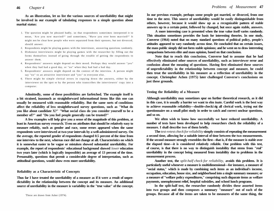
46 Chapter 4

As an illustration, let us list the various sources of unreliability that might be involved in our example of tabulating responses to a simple question about marital status:

1. T h e ques t ion migh t be phrased badly, so that r e sponden t s s o m e t i m e s interpreted i t to

mean , ' A r e you n o w m a r r i e d ? " and s o m e t i m e s , " H a v e you ever been m a r r i e d ? " I t

m igh t not be c lear h o w peop le w h o w e r e separa ted from their spouses , but not d ivorced,

shou ld answer .

2 . Respondents might be playing games with the interviewer, answer ing quest ions randomly.

3 . D i shones t in te rv iewers migh t be p lay ing g a m e s wi th the researcher by filling out the

forms themse lves ins tead of go ing through the t rouble of get t ing the r e sponden t s to

answer them.

4 . R e s p o n d e n t s ' an swer s migh t d e p e n d on their m o o d . Pe rhaps they wou ld a n s w e r " y e s "

w h e n they had had a good day, or " n o " w h e n they had had a bad day.

5 . R e s p o n d e n t s ' an swer s migh t depend on the context of the interview. A person migh t

say " n o " to an at t ract ive in te rv iewer and " y e s " to eve ryone e lse .

6 . T h e r e m i g h t be s imple c ler ical e r rors in c o p y i n g d o w n the a n s w e r s , e i ther by the

in te rv iewer on the spot or by the pe r son w h o t ranscr ibes the i n t e rv i ewer s ' copy in to a

compute r .

Admittedly, some of these possibilities are farfetched. The example itself is a bit strained, inasmuch as straightforward informational items like this one can usually be measured with reasonable reliability. But the same sorts of conditions affect the reliability of less straightforward survey questions, such as "What do you like about candidate X?" "What social class do you consider yourself to be a member of?" and "Do you feel people generally can be trusted?"

A few examples will help give you a sense of the magnitude of this problem, at least in American survey research.3 Even on attributes that should be relatively easy to measure reliably, such as gender and race, some errors appeared when the same respondents were interviewed at two-year intervals by a well-administered survey. On the average, the reported gender of respondents changed 0.5 percent of the time from one interview to the next, whereas race did not change at all. Characteristics on which it is somewhat easier to be vague or mistaken showed substantial unreliability. For example, the report of respondents' educational background showed lower education two years later (which is logically impossible) an average of 13 percent of the time. Presumably, questions that permit a considerable degree of interpretation, such as attitudinal questions, would show even more unreliability.

Reliability as a Characteristic of Concepts

Thus far I have treated the unreliability of a measure as if it were a result of unpre­dictability in the relationship between the concept and its measure. An additional source of unreliability in the measure is variability in the "true value" of the concept.

3 These are drawn from Asher (1974).

Problems of Measurement 47

In our previous example, perhaps some people got married, or divorced, from one time to the next. This source of unreliability would be easily distinguishable from others, however, because it would show up as a recognizable pattern of stable answers up to a certain point, followed by changed, but once again stable, answers.

A more interesting case is presented when the true value itself varies randomly. This situation sometimes provides the basis for interesting theories. In one study, Converse (1964) noted that on many standard questions of political policy, people's attitudes appeared to vary randomly across time. He concluded that on certain issues, the mass public simply did not form stable opinions; and he went on to draw interesting comparisons between elite and mass opinion, based on that conclusion.

Note that to reach this conclusion, Converse had to assume that he had effectively eliminated other sources of unreliability, such as interviewer error and confusion about the meaning of questions. Having first eliminated these sources of unpredictability in the relationship between concept and measure, he could then treat the unreliability in his measure as a reflection of unreliability in the concept. Christopher Achen (1975) later challenged Converse's conclusions on just these grounds.

Testing the Reliability of a Measure

Although unreliability may sometimes spur on further theoretical research, as it did in this case, it is usually a barrier we want to elm inate. Careful work is the best way to achieve reasonable reliability—double-checki rig all clerical work, trying out the questionnaire on a small pilot study in order to catch and correct unclear questions, and so on.

We often wish to know how successfully we have reduced unreliability. A number of tests have been developed to help researchers check the reliability of a measure. I shall describe two of them briefly.

The test-retest check for reliability simply consists of repeating the measurement a second time, allowing for a suitable interval of time between the two measurements. If the second measure strongly resembles the first—that is, if the measure is stable over the elapsed time—it is considered relatively reliable. One problem with this test, of course, is that there is no way to distinguish instability that stems from "real" unreliability in the concept being measured from instability due to problems in the measurement process.

Another test, the split-half check for reliability, avoids this problem. It is particularly useful whenever a measure is multidimensional—for instance, a measure of "social status," which is made by combining such items as an individual's income, occupation, education, house size, and neighborhood into a single summary measure; or a measure of "welfare policy expenditures," comprising such disparate items as welfare payments, unemployment relief, hospital subsidies, and school lunch programs.

In the split-half test, the researcher randomly divides these assorted items into two groups and then composes a summary "measure" out of each of the groups. Because all of the items are taken to be measures of the same thing, the

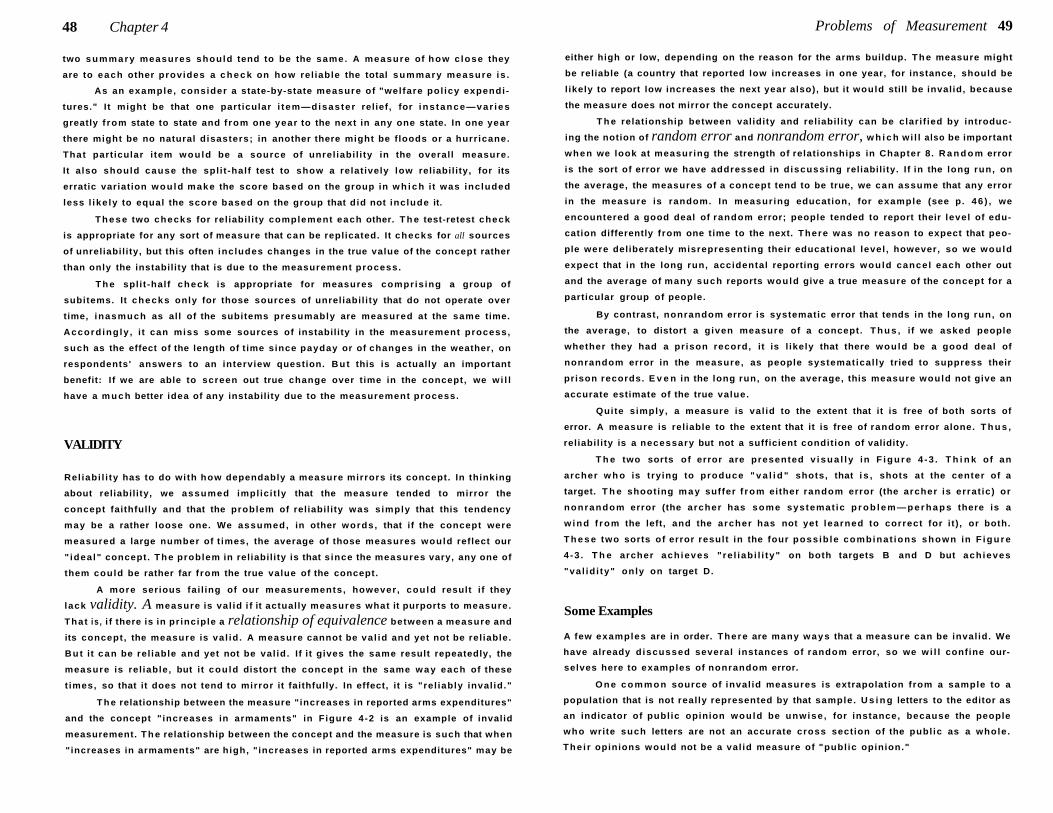
48 Chapter 4

two summary measures should tend to be the same. A measure of how c lose they

are to each other provides a c h e c k on how rel iable the total summary measure is .

As an example , consider a state-by-state measure of "welfare pol icy expendi­

tures." It might be that one particular i tem—disaster relief, for ins tance—var ies

greatly f rom state to state and f rom one year to the next in any one state. In one year

there might be no natural disasters; in another there might be floods or a hurr icane.

That particular i tem wou ld be a source of unrel iabil i ty in the overall measure.

It also should cause the spl i t -half test to show a relatively low reliability, for its

erratic variation wou ld make the score based on the group in w h i c h it was included

less l ike ly to equal the score based on the group that did not include it.

T h e s e two checks for reliabil ity complement each other. T h e test-retest check

is appropriate for any sort of measure that can be replicated. It checks for all sources

of unreliability, but this often includes changes in the true value of the concept rather

than only the instability that is due to the measurement process.

T h e spli t -half check is appropriate for measures compris ing a group of

subitems. It checks only for those sources of unreliabil i ty that do not operate over

time, inasmuch as al l of the subitems presumably are measured at the same time.

Accord ing ly , i t can miss some sources of instability in the measurement process,

such as the effect of the length of t ime since payday or of changes in the weather, on

respondents' answers to an interview question. B u t this is actually an important

benefit: If we are able to screen out true change over t ime in the concept, we w i l l

have a m u c h better idea of any instability due to the measurement process.

VALIDITY

Rel iabi l i ty has to do with how dependably a measure mirrors its concept. In thinking

about reliability, we assumed implici t ly that the measure tended to mirror the

concept faithfully and that the problem of reliabil ity was s imply that this tendency

may be a rather loose one. We assumed, in other words, that if the concept were

measured a large number of t imes, the average of those measures would reflect our

" idea l" concept. T h e problem in reliabil ity is that s ince the measures vary, any one of

them could be rather far f rom the true value of the concept.

A more serious fai l ing of our measurements, however, cou ld result i f they

lack validity. A measure is val id i f it actually measures what it purports to measure.

That is , i f there is in pr inciple a relationship of equivalence between a measure and

its concept, the measure is val id . A measure cannot be va l id and yet not be rel iable.

B u t it can be rel iable and yet not be val id. If i t gives the same result repeatedly, the

measure is rel iable, but it cou ld distort the concept in the same w a y each of these

t imes, so that it does not tend to mirror it faithfully. In effect, it is "rel iably inval id."

T h e relationship between the measure "increases in reported arms expenditures"

and the concept "increases in armaments" in Figure 4-2 is an example of invalid

measurement. T h e relationship between the concept and the measure is such that when

"increases in armaments" are high, "increases in reported arms expenditures" may be

Problems of Measurement 49

either high or low, depending on the reason for the arms buildup. T h e measure might

be reliable (a country that reported low increases in one year, for instance, should be

l ikely to report low increases the next year also), but it would still be invalid, because

the measure does not mirror the concept accurately.

T h e relationship between validity and reliabil ity can be clarif ied by introduc­

ing the notion of random error and nonrandom error, w h i c h wi l l also be important

when we look at measuring the strength of relationships in Chapter 8. R a n d o m error

is the sort of error we have addressed in d iscussing reliability. I f in the long run, on

the average, the measures of a concept tend to be true, we can assume that any error

in the measure is random. In measur ing education, for example (see p. 46 ) , we

encountered a good deal of random error; people tended to report their level of edu­

cation differently from one time to the next. There was no reason to expect that peo­

ple were deliberately misrepresenting their educational level , however, so we would

expect that in the long run, accidental reporting errors would cancel each other out

and the average of many such reports would give a true measure of the concept for a

particular group of people.

By contrast, nonrandom error is systematic error that tends in the long run, on

the average, to distort a given measure of a concept. T h u s , if we asked people

whether they had a pr ison record, it is l ikely that there would be a good deal of

nonrandom error in the measure, as people systematical ly tried to suppress their

prison records. E v e n in the long run, on the average, this measure would not give an

accurate estimate of the true value.

Quite simply, a measure is val id to the extent that it is free of both sorts of

error. A measure is reliable to the extent that it is free of random error alone. T h u s ,

reliabil ity is a necessary but not a sufficient condition of validity.

T h e two sorts of error are presented v i s u a l l y in F i g u r e 4 -3 . T h i n k of an

archer w h o is trying to produce " v a l i d " shots, that i s , shots at the center of a

target. T h e shooting m a y suffer f rom either random error (the archer is errat ic) or

nonrandom error (the archer has some systemat ic p r o b l e m — p e r h a p s there is a

w i n d f rom the left, and the archer has not yet learned to correct for i t) , or both.

T h e s e two sorts of error result in the four poss ib le combinat ions shown in F i g u r e

4 -3 . T h e archer ach ieves "re l iab i l i ty" on both targets B and D but ach ieves

"va l id i ty" only on target D.

Some Examples

A few examples are in order. There are many ways that a measure can be inval id. We

have already d iscussed several instances of random error, so we wi l l confine our­

selves here to examples of nonrandom error.

O n e c o m m o n source of inval id measures is extrapolation from a sample to a

population that is not real ly represented by that sample. U s i n g letters to the editor as

an indicator of publ ic opinion would be unwise , for instance, because the people

who write such letters are not an accurate cross section of the publ ic as a whole.

The i r opinions would not be a val id measure of "publ ic opinion."

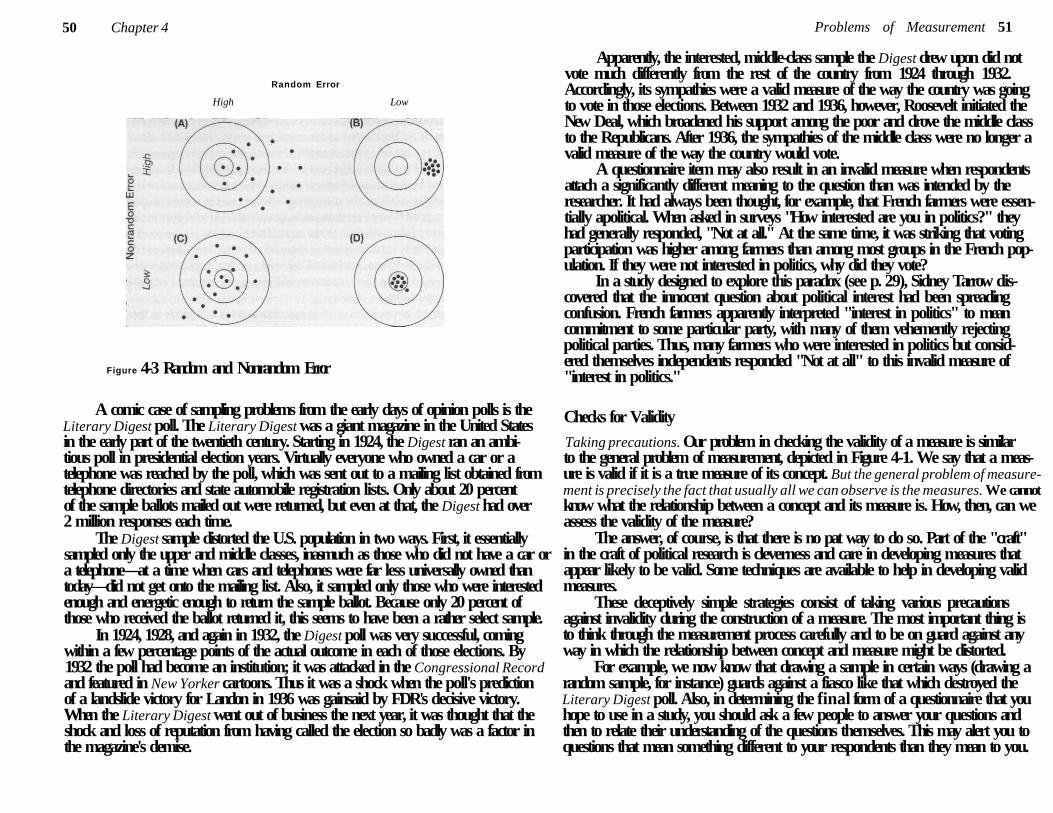
50 Chapter 4

Random Error

High Low

Figure 4-3 Random and Nonrandom Error

A comic case of sampling problems from the early days of opinion polls is the Literary Digest poll. The Literary Digest was a giant magazine in the United States in the early part of the twentieth century. Starting in 1924, the Digest ran an ambi­tious poll in presidential election years. Virtually everyone who owned a car or a telephone was reached by the poll, which was sent out to a mailing list obtained from telephone directories and state automobile registration lists. Only about 20 percent of the sample ballots mailed out were returned, but even at that, the Digest had over 2 million responses each time.

The Digest sample distorted the U.S. population in two ways. First, it essentially sampled only the upper and middle classes, inasmuch as those who did not have a car or a telephone—at a time when cars and telephones were far less universally owned than today—did not get onto the mailing list. Also, it sampled only those who were interested enough and energetic enough to return the sample ballot. Because only 20 percent of those who received the ballot returned it, this seems to have been a rather select sample.

In 1924, 1928, and again in 1932, the Digest poll was very successful, coming within a few percentage points of the actual outcome in each of those elections. By 1932 the poll had become an institution; it was attacked in the Congressional Record and featured in New Yorker cartoons. Thus it was a shock when the poll's prediction of a landslide victory for Landon in 1936 was gainsaid by FDR's decisive victory. When the Literary Digest went out of business the next year, it was thought that the shock and loss of reputation from having called the election so badly was a factor in the magazine's demise.

Problems of Measurement 51

Apparently, the interested, middle-class sample the Digest drew upon did not vote much differently from the rest of the country from 1924 through 1932. Accordingly, its sympathies were a valid measure of the way the country was going to vote in those elections. Between 1932 and 1936, however, Roosevelt initiated the New Deal, which broadened his support among the poor and drove the middle class to the Republicans. After 1936, the sympathies of the middle class were no longer a valid measure of the way the country would vote.

A questionnaire item may also result in an invalid measure when respondents attach a significantly different meaning to the question than was intended by the researcher. It had always been thought, for example, that French farmers were essen­tially apolitical. When asked in surveys "How interested are you in politics?" they had generally responded, "Not at all." At the same time, it was striking that voting participation was higher among farmers than among most groups in the French pop­ulation. If they were not interested in politics, why did they vote?

In a study designed to explore this paradox (see p. 29), Sidney Tarrow dis­covered that the innocent question about political interest had been spreading confusion. French farmers apparently interpreted "interest in politics" to mean commitment to some particular party, with many of them vehemently rejecting political parties. Thus, many farmers who were interested in politics but consid­ered themselves independents responded "Not at all" to this invalid measure of "interest in politics."

Checks for Validity Taking precautions. Our problem in checking the validity of a measure is similar to the general problem of measurement, depicted in Figure 4-1. We say that a meas­ure is valid if it is a true measure of its concept. But the general problem of measure­ment is precisely the fact that usually all we can observe is the measures. We cannot know what the relationship between a concept and its measure is. How, then, can we assess the validity of the measure?

The answer, of course, is that there is no pat way to do so. Part of the "craft" in the craft of political research is cleverness and care in developing measures that appear likely to be valid. Some techniques are available to help in developing valid measures.

These deceptively simple strategies consist of taking various precautions against invalidity during the construction of a measure. The most important thing is to think through the measurement process carefully and to be on guard against any way in which the relationship between concept and measure might be distorted.

For example, we now know that drawing a sample in certain ways (drawing a random sample, for instance) guards against a fiasco like that which destroyed the Literary Digest poll. Also, in determining the final form of a questionnaire that you hope to use in a study, you should ask a few people to answer your questions and then to relate their understanding of the questions themselves. This may alert you to questions that mean something different to your respondents than they mean to you.

52 Chapter 4

S u c h prel iminary testing of one's measures is cal led a "pilot study." Simi lar ly , in

using off icial documents, you should go thoroughly into the background of the

things reported there—how they were developed, what the terms mean, how broadly

they are intended to apply, and so on.

T h e s e techniques s imply require that the investigator think ahead to problems

that could occur in the relationship between concept and measure and act either to

prevent these or to check to see whether they are present. At the most general level ,

the strategy I have suggested here requires only that the investigator consider care­

fully how plausible it is that the measure mirrors the concept.

Test of validity. T h u s far our strategies have not actually provided a test of the

validity of the measure. S u c h a test can be made, although it is necessari ly subjective

and open to varying interpretations. L e t us say that we want to decide whether

measure a is a val id measure of concept A. If there is some measure /3 that we are

certain is strongly related to concept A, we can check to see whether measure j i is

related to measure a. If it is not, and our assumption of a relationship between /3 and

A is true, then a could not be a val id measure of A.

T h e study by Tarrow cited earlier provides an example of this logic. Tarrow's

initial conclusion that the usual question " H o w interested are you in po l i t ics?" was

providing an invalid measure of "polit ical interest" among F rench farmers came

from his observation that farmers had in fact one of the highest levels of electoral

participation among F r e n c h cit izens. B e c a u s e he could not conceive of high electoral

participation occurring in the absence of high polit ical interest, he concluded that the

conventional measures, w h i c h had showed low polit ical interest coincid ing with high

participation, must not have been measuring polit ical interest val id ly . 4

As another example of this k ind of test, consider a measure of nations' hostility

to each other—based on content analysis of the nations' newspapers ( a ) . I f we found

that two of the nations went to war against each other (/3) yet the measure did not

show an accompanying increase in feelings of hostility between the two, we would be

suspicious of the validity of the measures.

S u c h an indirect test of validity is possible only when a researcher is quite

certain that /3 must go along with A. That kind of certainty is uncommon and

may not be shared equally by every observer. T h u s , this test is not a lways , or even

usually, possible; and it is a lways rather subjective. But assessing the validity of

measures is so important that an indirect test, when it can be used, w i l l greatly

strengthen your f indings.

T h e most general test of validity is what is cal led face validity. T h i s is just a

fancy term for whether a measure looks right to you. Is it val id "on its f a c e " ? After

a l l , you have considerable experience with polit ics and must judge for yoursel f

whether the measure does what you want it to do. If you think it does (and people

w h o read your work agree with you) , i t has face validity.

4 In this example, "political interest" corresponds to A, farmers' responses to the question on polit­ical interest correspond to a, and farmers' electoral participation corresponds to B.

Problems of Measurement 53

I M P A C T O F R A N D O M A N D N O N R A N D O M E R R O R S

It should be obvious that the only good measure is one that is val id, that is , one that

has in it neither random nor nonrandom error. B e c a u s e socia l scientists often operate

with measures that suffer f rom one or the other sort of error, however, it is worth

considering what happens under those c i rcumstances. As it happens, the two sorts of

error have different effects on the development of theory.

T h e effect of nonrandom error is simple and severe. I f a measure is systemati ­

cal ly inval id, there is no reason for us to expect any correspondence between the

relationship we actually observe from our measures and the ideal ized relationship

we w i s h to investigate.

T h e effect of unreliabil i ty ( i f the measures are otherwise valid) is more subtle.

To the extent that measures are unreliable, the relationship at the measure level

w i l l tend to be looser and weaker than the true relationship. It w i l l paral lel the true

relationship but w i l l appear weaker than is actually the case. If the measures are

sufficiently unrel iable, the basic relationship can be so weakened that it w i l l appear,

from what we can observe, as if there is no relationship at al l .

T h i s is illustrated in Table 4-1. E a c h set of two columns tabulates the closeness

of elections in ten congressional districts, as well as their representatives' seniority. It

is apparent from the figures in the first set of columns (True Values) that there is a

relationship between the two, inasmuch as representatives from safe districts tend to

have greater seniority than those from marginal districts. T h e relationship is also quite

strong; seniority increases without exception as the representatives' margins of victory

increase.

In the third and fourth columns, random error, such as might occur from clerical

errors or other sources of unreliability, has been added to the original measures,

making them less reliable. In the fifth and sixth columns, an even greater degree of

TABLE 4-1 Safe Districts Related to Seniority, Using Simulated Data

True Values Less Reliable Measures Very Unreliable Measures

Seniority Margin of Victory (%) Seniority

Margin of Victory (%) Seniority

Margin of Victory (%)

32 18 32.0 21.6 12.8 9.0

24 12 19.2 12.0 12.0 12.6

23 1 1 11.5 12.1 30.2 8.8

20 11 22.0 4.4 22.4 6.6

14 8 14.0 5.6 21.2 12.0

11 6 11.0 6.0 13.1 3.6

10 6 9.0 10.8 2.5 0.1

6 4 3.6 4.0 13.8 2.8

5 3 4.5 3.6 21.3 1.5

2 1 2.4 0.5 0.2 12.9

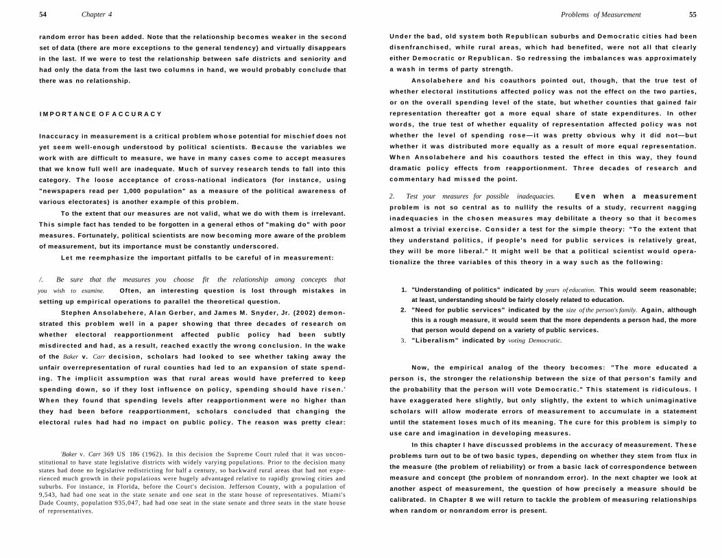
54 Chapter 4

random error has been added. Note that the relationship becomes weaker in the second

set of data (there are more exceptions to the general tendency) and virtually disappears

in the last. If we were to test the relationship between safe districts and seniority and

had only the data from the last two columns in hand, we would probably conclude that

there was no relationship.

I M P O R T A N C E O F A C C U R A C Y

Inaccuracy in measurement is a crit ical problem whose potential for mischief does not

yet seem wel l -enough understood by political scientists. B e c a u s e the variables we

work with are difficult to measure, we have in many cases come to accept measures

that we know full wel l are inadequate. M u c h of survey research tends to fall into this

category. T h e loose acceptance of cross-national indicators (for instance, using

"newspapers read per 1,000 population" as a measure of the political awareness of

various electorates) is another example of this problem.

To the extent that our measures are not valid, what we do with them is irrelevant.

Th is simple fact has tended to be forgotten in a general ethos of "making do" with poor

measures. Fortunately, political scientists are now becoming more aware of the problem

of measurement, but its importance must be constantly underscored.

L e t me reemphasize the important pitfalls to be careful of in measurement:

/. Be sure that the measures you choose fit the relationship among concepts that

you wish to examine. Often, an interesting question is lost through mistakes in

setting up empir ical operations to parallel the theoretical question.

Stephen Ansolabehere , A l a n Gerber , and James M. Snyder , Jr. (2002) demon­

strated this problem wel l in a paper showing that three decades of research on

whether electoral reapportionment affected publ ic pol icy had been subtly

misdirected and had, as a result, reached exact ly the wrong conc lus ion . In the wake

of the Baker v. Carr dec is ion , scholars had looked to see whether taking away the

unfair overrepresentation of rural counties had led to an expansion of state spend­

ing. T h e impl ic i t assumption was that rural areas would have preferred to keep

spending down, so i f they lost inf luence on pol icy, spending should have r i s e n . 5

W h e n they found that spending levels after reapportionment were no higher than

they had been before reapportionment, scholars concluded that changing the

electoral rules had had no impact on publ ic pol icy. T h e reason was pretty clear:

5Baker v. Carr 369 US 186 (1962). In this decision the Supreme Court ruled that it was uncon­stitutional to have state legislative districts with widely varying populations. Prior to the decision many states had done no legislative redistricting for half a century, so backward rural areas that had not expe­rienced much growth in their populations were hugely advantaged relative to rapidly growing cities and suburbs. For instance, in Florida, before the Court's decision. Jefferson County, with a population of 9,543, had had one seat in the state senate and one seat in the state house of representatives. Miami's Dade County, population 935,047, had had one seat in the state senate and three seats in the state house of representatives.

Problems of Measurement 55

Under the bad, old system both Repub l ican suburbs and Democra t ic cit ies had been

disenfranchised, whi le rural areas, w h i c h had benefited, were not al l that c lear ly

either Democra t ic or Repub l i can . So redressing the imbalances was approximately

a wash in terms of party strength.

Anso labehere and h is coauthors pointed out, though, that the true test of

whether electoral institutions affected pol icy was not the effect on the two parties,

or on the overal l spending level of the state, but whether counties that gained fair

representation thereafter got a more equal share of state expenditures. In other

words , the true test of whether equali ty of representation affected po l icy w a s not

whether the level of spending r o s e — i t was pretty obvious w h y i t did not—but

whether it was distributed more equal ly as a result of more equal representation.

W h e n Ansolabehere and his coauthors tested the effect in this way, they found

dramatic pol icy effects f rom reapportionment. T h r e e decades of research and

commentary had missed the point.

2. Test your measures for possible inadequacies. E v e n w h e n a measurement

problem is not so central as to nul l i fy the results of a study, recurrent nagging

inadequacies in the chosen measures may debilitate a theory so that it becomes

almost a tr ivial exerc ise . C o n s i d e r a test for the s imple theory: "To the extent that

they understand pol i t ics, i f people 's need for publ ic serv ices is relat ively great,

they w i l l be more l iberal ." It might wel l be that a pol i t ical scientist wou ld opera-

t ional ize the three variables of this theory in a w a y such as the fo l lowing:

1. "Understanding of politics" indicated by years of education. This would seem reasonable;

at least, understanding should be fairly closely related to education.

2. "Need for public services" indicated by the size of the person's family. Again, although

this is a rough measure, it would seem that the more dependents a person had, the more

that person would depend on a variety of public services.

3. "Liberalism" indicated by voting Democratic.

Now, the empir ical analog of the theory becomes: " T h e more educated a

person is , the stronger the relationship between the size of that person's family and

the probability that the person w i l l vote Democrat ic ." T h i s statement is r idiculous. I

have exaggerated here slightly, but only slightly, the extent to w h i c h unimaginative

scholars wi l l al low moderate errors of measurement to accumulate in a statement

until the statement loses m u c h of its meaning. T h e cure for this problem is s imply to

use care and imagination in developing measures.

In this chapter I have discussed problems in the accuracy of measurement. These

problems turn out to be of two basic types, depending on whether they stem from flux in

the measure (the problem of reliability) or from a basic lack of correspondence between

measure and concept (the problem of nonrandom error). In the next chapter we look at

another aspect of measurement, the question of how precisely a measure should be

calibrated. In Chapter 8 we wi l l return to tackle the problem of measuring relationships

when random or nonrandom error is present.

56 Chapter 4

F U R T H E R D I S C U S S I O N

A delightful book with a unique approach to handling certain problems of validity is

Unobtrusive Measures, by Eugene J. Webb, Donald T. Campbel l , R ichard D. Schwartz,

and L e e Sechrist (1966). T h e ideas presented in the book are both creative and

sound, and the text itself is filled with interesting and highly unusual examples.

Frederick Mosteller's article "Errors ," in the International Encyclopedia of the Social

Sciences (1968), is wel l worth reading. Mosteller details a variety of possible sources of

invalidity and unreliability. Herbert Asher (1974) presents some good examples of

reliability problems, with a rather technical discussion of ways to handle them. See also

K i r k and Miller, Reliability and Validity in Qualitative Research (1985).

Several good examples of specific measurement problems are Niemi and

Krehbie l (1984), "The Quality of Surveying Responses About Parents and the Fami ly" ;

Hammond and Fraser (1984), "Studying Presidential Performance in Congress":

Fe ldman (1983), "The Measurement and Meaning of Trust in Government"; and

Converse and Pierce (1985), "Measuring Partisanship."

A usefu l exerc ise w o u l d be to l ist as many factors as y o u can that w o u l d lead

to random or nonrandom error for each of the fo l lowing measures: intended vote

( in s u r v e y s ) ; strength of armed forces; agreement wi th the president ( in congres­

sional vot ing); t r ibal ism; unemployment ; h ierarch ica l control in an agency; and

personal income.

Chapter 5

D

Precision

T h e preceding chapter dealt with problems of the reliabil ity and validity of

measures. T h o s e problems concerned the relationship between a measure and the

concept that measure is intended to mirror. In this chapter we deal with the "qual i ty"

of the measure i tse l f—how precise it should be, or how finely calibrated, if it is to

be useful .

In a study of Norwegian pol i t ics, Harry E c k s t e i n felt that it was necessary to

apologize for the fact that some measures he would use were subjective intangibles

("warmth in socia l relations," for instance, and "sense of communi ty" ) rather than

precise numerical quantities.

[M]any of the indicators used in the text may not be readily recognized as such by

contemporary social scientists. By an indicator we usually mean nowadays a precisely

ascertainable quantity that stands for some imprecise quantity (as GNP may indicate

level of economic development, or as the number of casualties in revolutionary

violence may indicate its intensity). I do use such quantities in what follows. More

often, however, readily observable "qualities" are used as indicators of not-so-readily

observable qualities. This strikes me as both defensible and desirable, for quantitative

indicators are not always as "indicative" of what one wants to know as other observa­

tions, nor always obtainable. In overemphasizing quantities we sometimes miss the

most telling data—in any case, data that may be reliable in their own right or used as

checks on the inferences drawn from quantitative data. I conceive of all social behavior

as a vast "data bank," only some of which is quantitatively aggregated in yearbooks and

the like, and much of the rest of which may speak volumes to our purposes, if used

circumspectly. (Eckstein, 1966, footnote pp. 79-80) 1

'From Eckstein, Harry, Division and Cohesion in Democracy: A Study of Norway (Copyright 1966 by Princeton University Press). Reprinted by permission of Princeton University Press.

57

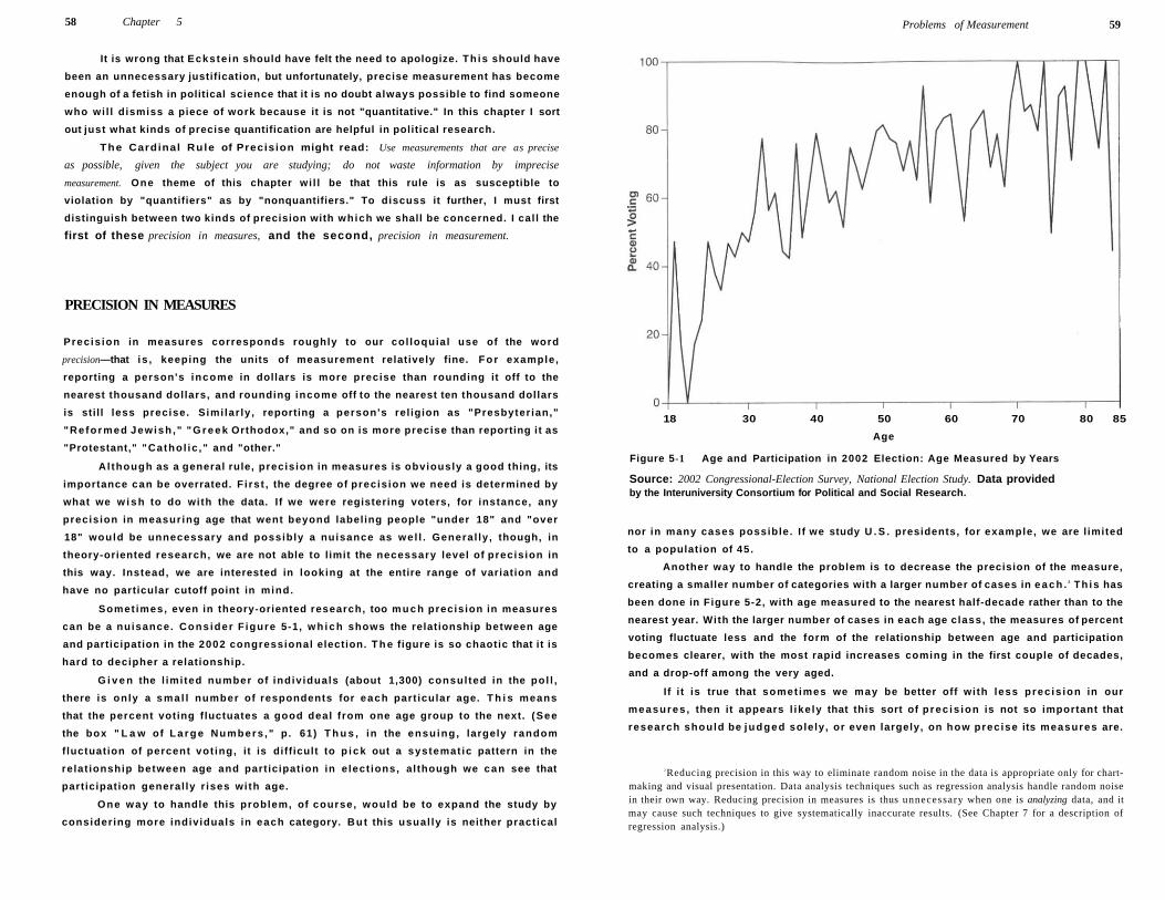
58 Chapter 5

It is wrong that Eckste in should have felt the need to apologize. Th is should have

been an unnecessary justification, but unfortunately, precise measurement has become

enough of a fetish in political science that it is no doubt always possible to find someone

who wi l l dismiss a piece of work because it is not "quantitative." In this chapter I sort

out just what kinds of precise quantification are helpful in political research.

The Cardinal Rule of Precision might read: Use measurements that are as precise

as possible, given the subject you are studying; do not waste information by imprecise

measurement. One theme of this chapter wi l l be that this rule is as susceptible to

violation by "quantifiers" as by "nonquantifiers." To discuss it further, I must first

distinguish between two kinds of precision with which we shall be concerned. I cal l the

first of these precision in measures, and the second, precision in measurement.

PRECISION IN MEASURES

Precis ion in measures corresponds roughly to our col loquial use of the word

precision—that is , keeping the units of measurement relatively fine. F o r example,

reporting a person's income in dollars is more precise than rounding it off to the

nearest thousand dollars, and rounding income off to the nearest ten thousand dollars

is stil l less precise. Simi lar ly , reporting a person's rel igion as "Presbyter ian,"

"Reformed Jewish ," " G r e e k Orthodox," and so on is more precise than reporting it as

"Protestant," "Cathol ic , " and "other."

A l though as a general rule, precision in measures is obviously a good thing, its

importance can be overrated. F i rs t , the degree of precis ion we need is determined by

what we w i s h to do with the data. I f we were registering voters, for instance, any

precision in measur ing age that went beyond labeling people "under 18" and "over

18" would be unnecessary and possibly a nuisance as we l l . General ly , though, in

theory-oriented research, we are not able to l imit the necessary level of precis ion in

this way. Instead, we are interested in looking at the entire range of variation and

have no particular cutoff point in mind.

Somet imes, even in theory-oriented research, too m u c h precision in measures

can be a nuisance. Cons ider F igure 5-1, w h i c h shows the relationship between age

and participation in the 2002 congressional election. T h e figure is so chaotic that it is

hard to decipher a relationship.

G i v e n the l imited number of indiv iduals (about 1,300) consul ted in the pol l ,

there is only a sma l l number of respondents for each part icular age. T h i s means

that the percent voting fluctuates a good deal f rom one age group to the next. (See

the box " L a w of L a r g e Numbers , " p . 61) T h u s , in the ensuing , largely random

fluctuation of percent vot ing, it is diff icult to p i c k out a systemat ic pattern in the

relat ionship between age and part icipation in e lect ions, al though we can see that

participation general ly r ises wi th age.

One w a y to handle this problem, of course, would be to expand the study by

considering more individuals in each category. B u t this usual ly is neither practical

Problems of Measurement 59

18 30 40 50 60 70 80 85

Age

Figure 5-1 Age and Participation in 2002 Election: Age Measured by Years

Source: 2002 Congressional-Election Survey, National Election Study. Data provided by the Interuniversity Consortium for Political and Social Research.

nor in many cases possible. I f we study U . S . presidents, for example, we are l imited

to a population of 45.

Another way to handle the problem is to decrease the precision of the measure,

creating a smaller number of categories with a larger number of cases in e a c h . 2 Th is has

been done in Figure 5-2, with age measured to the nearest half-decade rather than to the

nearest year. With the larger number of cases in each age class, the measures of percent

voting fluctuate less and the form of the relationship between age and participation

becomes clearer, with the most rapid increases coming in the first couple of decades,

and a drop-off among the very aged.

I f i t is true that somet imes we may be better off with less prec is ion in our

measures , then it appears l ike ly that this sort of p rec is ion is not so important that

research should be judged solely, or even largely, on how precise its measures are.

2Reducing precision in this way to eliminate random noise in the data is appropriate only for chart-making and visual presentation. Data analysis techniques such as regression analysis handle random noise in their own way. Reducing precision in measures is thus unnecessary when one is analyzing data, and it may cause such techniques to give systematically inaccurate results. (See Chapter 7 for a description of regression analysis.)

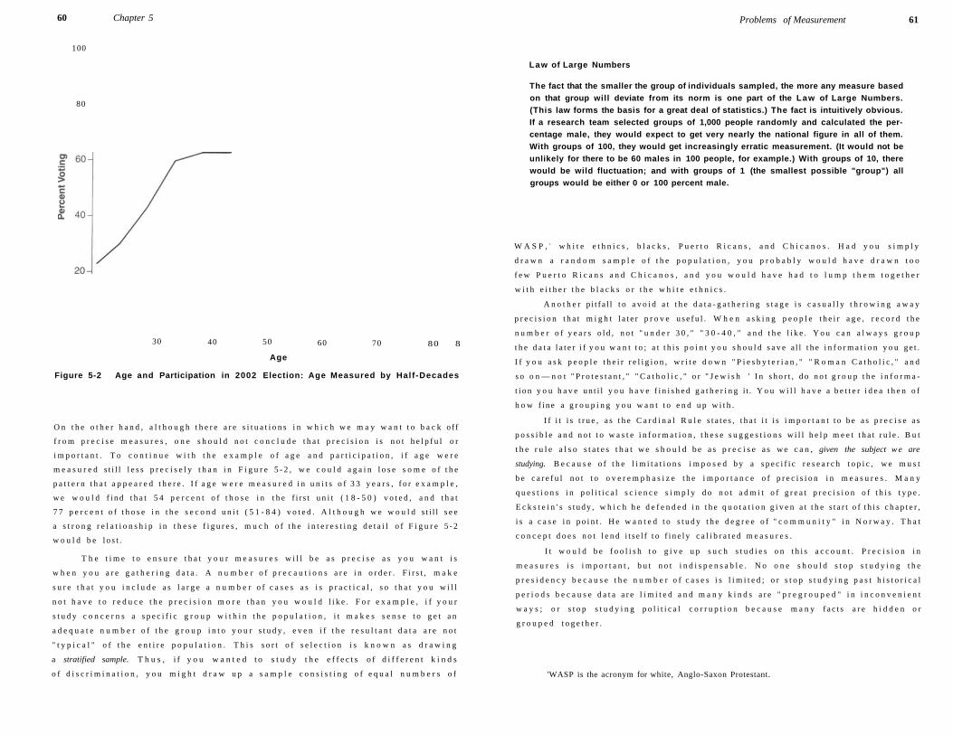
60 Chapter 5

100

80

30 40 50 60 70 80 8

Age

Figure 5-2 Age and Participation in 2002 Election: Age Measured by Half -Decades

O n t h e o t h e r h a n d , a l t h o u g h t h e r e a r e s i t u a t i o n s i n w h i c h w e m a y w a n t t o b a c k o f f

f r o m p r e c i s e m e a s u r e s , o n e s h o u l d n o t c o n c l u d e t h a t p r e c i s i o n i s n o t h e l p f u l o r

i m p o r t a n t . T o c o n t i n u e w i t h t h e e x a m p l e o f a g e a n d p a r t i c i p a t i o n , i f a g e w e r e

m e a s u r e d s t i l l l e s s p r e c i s e l y t h a n i n F i g u r e 5 - 2 , w e c o u l d a g a i n l o s e s o m e o f t h e

p a t t e r n t h a t a p p e a r e d t h e r e . I f a g e w e r e m e a s u r e d i n u n i t s o f 3 3 y e a r s , f o r e x a m p l e ,

w e w o u l d f i n d t h a t 5 4 p e r c e n t o f t h o s e i n t h e f i r s t u n i t ( 1 8 - 5 0 ) v o t e d , a n d t h a t

7 7 p e r c e n t o f t h o s e i n t h e s e c o n d u n i t ( 5 1 - 8 4 ) v o t e d . A l t h o u g h w e w o u l d s t i l l s e e

a s t r o n g r e l a t i o n s h i p i n t h e s e f i g u r e s , m u c h o f t h e i n t e r e s t i n g d e t a i l o f F i g u r e 5 - 2

w o u l d b e l o s t .

T h e t i m e t o e n s u r e t h a t y o u r m e a s u r e s w i l l b e a s p r e c i s e a s y o u w a n t i s

w h e n y o u a r e g a t h e r i n g d a t a . A n u m b e r o f p r e c a u t i o n s a r e i n o r d e r . F i r s t , m a k e

s u r e t h a t y o u i n c l u d e a s l a r g e a n u m b e r o f c a s e s a s i s p r a c t i c a l , s o t h a t y o u w i l l

n o t h a v e t o r e d u c e t h e p r e c i s i o n m o r e t h a n y o u w o u l d l i k e . F o r e x a m p l e , i f y o u r

s t u d y c o n c e r n s a s p e c i f i c g r o u p w i t h i n t h e p o p u l a t i o n , i t m a k e s s e n s e t o g e t a n

a d e q u a t e n u m b e r o f t h e g r o u p i n t o y o u r s t u d y , e v e n i f t h e r e s u l t a n t d a t a a r e n o t

" t y p i c a l " o f t h e e n t i r e p o p u l a t i o n . T h i s s o r t o f s e l e c t i o n i s k n o w n a s d r a w i n g

a stratified sample. T h u s , i f y o u w a n t e d t o s t u d y t h e e f f e c t s o f d i f f e r e n t k i n d s

o f d i s c r i m i n a t i o n , y o u m i g h t d r a w u p a s a m p l e c o n s i s t i n g o f e q u a l n u m b e r s o f

Problems of Measurement 61

Law of Large Numbers

The fact that the smaller the group of individuals sampled, the more any measure based on that group will deviate from its norm is one part of the Law of Large Numbers. (This law forms the basis for a great deal of statistics.) The fact is intuitively obvious. If a research team selected groups of 1,000 people randomly and calculated the per­centage male, they would expect to get very nearly the national figure in all of them. With groups of 100, they would get increasingly erratic measurement. (It would not be unlikely for there to be 60 males in 100 people, for example.) With groups of 10, there would be wild fluctuation; and with groups of 1 (the smallest possible "group") all groups would be either 0 or 100 percent male.

W A S P , 3 w h i t e e t h n i c s , b l a c k s , P u e r t o R i c a n s , a n d C h i c a n o s . H a d y o u s i m p l y

d r a w n a r a n d o m s a m p l e o f t h e p o p u l a t i o n , y o u p r o b a b l y w o u l d h a v e d r a w n t o o

f e w P u e r t o R i c a n s a n d C h i c a n o s , a n d y o u w o u l d h a v e h a d t o l u m p t h e m t o g e t h e r

w i t h e i t h e r t h e b l a c k s o r t h e w h i t e e t h n i c s .

A n o t h e r p i t f a l l t o a v o i d a t t h e d a t a - g a t h e r i n g s t a g e i s c a s u a l l y t h r o w i n g a w a y

p r e c i s i o n t h a t m i g h t l a t e r p r o v e u s e f u l . W h e n a s k i n g p e o p l e t h e i r a g e , r e c o r d t h e

n u m b e r o f y e a r s o l d , n o t " u n d e r 3 0 , " " 3 0 - 4 0 , " a n d t h e l i k e . Y o u c a n a l w a y s g r o u p

t h e d a t a l a t e r i f y o u w a n t t o ; a t t h i s p o i n t y o u s h o u l d s a v e a l l t h e i n f o r m a t i o n y o u g e t .

I f y o u a s k p e o p l e t h e i r r e l i g i o n , w r i t e d o w n " P i e s b y t e r i a n , " " R o m a n C a t h o l i c , " a n d

s o o n — n o t " P r o t e s t a n t , " " C a t h o l i c , " o r " J e w i s h ' I n s h o r t , d o n o t g r o u p t h e i n f o r m a ­

t i o n y o u h a v e u n t i l y o u h a v e f i n i s h e d g a t h e r i n g i t . Y o u w i l l h a v e a b e t t e r i d e a t h e n o f

h o w f i n e a g r o u p i n g y o u w a n t t o e n d u p w i t h .

I f i t i s t r u e , a s t h e C a r d i n a l R u l e s t a t e s , t h a t i t i s i m p o r t a n t t o b e a s p r e c i s e a s

p o s s i b l e a n d n o t t o w a s t e i n f o r m a t i o n , t h e s e s u g g e s t i o n s w i l l h e l p m e e t t h a t r u l e . B u t

t h e r u l e a l s o s t a t e s t h a t we s h o u l d be a s p r e c i s e a s we c a n , given the subject we are

studying. B e c a u s e o f t h e l i m i t a t i o n s i m p o s e d b y a s p e c i f i c r e s e a r c h t o p i c , w e m u s t

b e c a r e f u l n o t t o o v e r e m p h a s i z e t h e i m p o r t a n c e o f p r e c i s i o n i n m e a s u r e s . M a n y

q u e s t i o n s i n p o l i t i c a l s c i e n c e s i m p l y d o n o t a d m i t o f g r e a t p r e c i s i o n o f t h i s t y p e .

E c k s t e i n ' s s t u d y , w h i c h h e d e f e n d e d i n t h e q u o t a t i o n g i v e n a t t h e s t a r t o f t h i s c h a p t e r ,

i s a c a s e i n p o i n t . H e w a n t e d t o s t u d y t h e d e g r e e o f " c o m m u n i t y " i n N o r w a y . T h a t

c o n c e p t d o e s n o t l e n d i t s e l f t o f i n e l y c a l i b r a t e d m e a s u r e s .

I t w o u l d b e f o o l i s h t o g i v e u p s u c h s t u d i e s o n t h i s a c c o u n t . P r e c i s i o n i n

m e a s u r e s i s i m p o r t a n t , b u t n o t i n d i s p e n s a b l e . N o o n e s h o u l d s t o p s t u d y i n g t h e

p r e s i d e n c y b e c a u s e t h e n u m b e r o f c a s e s i s l i m i t e d ; o r s t o p s t u d y i n g p a s t h i s t o r i c a l

p e r i o d s b e c a u s e d a t a a r e l i m i t e d a n d m a n y k i n d s a r e " p r e g r o u p e d " i n i n c o n v e n i e n t

w a y s ; o r s t o p s t u d y i n g p o l i t i c a l c o r r u p t i o n b e c a u s e m a n y f a c t s a r e h i d d e n o r

g r o u p e d t o g e t h e r .

'WASP is the acronym for white, Anglo-Saxon Protestant.

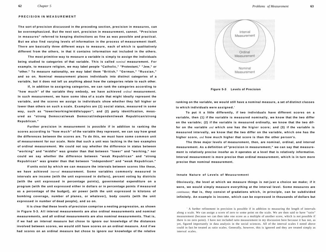
62 Chapter 5

P R E C I S I O N I N M E A S U R E M E N T

T h e sort of precision d iscussed in the preceding section, precision in measures, can

be overemphasized. But the next sort, precision in measurement, cannot. "Prec is ion

in measures" referred to keeping distinctions as fine as was possible and pract ical .

B u t we also f ind varying levels of information in the process of measurement itself.

There are basica l ly three different ways to measure, each of w h i c h is qualitatively

different f rom the others, in that it contains information not included in the others.

T h e most primitive way to measure a variable is simply to assign the individuals

being studied to categories of that variable. Th is is cal led nominal measurement. F o r

example, to measure religion, we may label people "Cathol ic ," "Protestant," "Jew," or

"other." To measure nationality, we may label them "Bri t ish," "German," " R u s s i a n , "

and so on. Nominal measurement places individuals into distinct categories of a

variable, but it does not tell us anything about how the categories relate to each other.

If, in addition to assigning categories, we can rank the categories according to

"how m u c h " of the variable they embody, we have achieved ordinal measurement.

In such measurement, we have some idea of a scale that might ideally represent the

variable, and the scores we assign to individuals show whether they fall higher or

lower than others on such a scale. E x a m p l e s are (1) social status, measured in some

way, such as " lower/working/middle/upper"; and (2) party identification, meas­

ured as "strong Democrat /weak Democrat / independent/weak Republ ican/strong

Republ ican ."

Further precision in measurement is possible if in addition to ranking the

scores according to "how m u c h " of the variable they represent, we can say how great

the differences between the scores are. To do this, we must have some c o m m o n unit

of measurement for our scale. Note that such a unit was lacking in the two examples

of ordinal measurement. We could not say whether the difference in status between

"work ing" and "middle" was greater than that between " lower" and "working," nor

could we say whether the difference between "weak R e p u b l i c a n " and "strong

R e p u b l i c a n " was greater than that between "independent" and "weak Republ ican ."

I f units exist by w h i c h we can measure the intervals between scores l ike these,

we have achieved interval measurement. S o m e variables commonly measured in

intervals are income (with the unit expressed in dol lars) , percent voting by districts

(with the unit expressed in percentage points), governmental expenditure on a

program (with the unit expressed either in dollars or in percentage points if measured

as a percentage of the budget), air power (with the unit expressed in kilotons of

bombing coverage, number of planes, or whatever) , body counts (with the unit

expressed in number of dead people) , and so on.

It is clear that these levels of precision comprise a nesting progression, as shown

in Figure 5-3. A l l interval measurements are also ordinal measurements and nominal

measurements, and all ordinal measurements are also nominal measurements. That is,

if we had an interval measure but chose to ignore our knowledge of the distances

involved between scores, we would still have scores on an ordinal measure. A n d if we

had scores on an ordinal measure but chose to ignore our knowledge of the relative

Problems of Measurement 63

Figure 5-3 Levels of Precision

ranking on the variable, we would still have a nominal measure, a set of distinct classes

to wh ich individuals were ass igned. 4

To put it a little differently, if two individuals have different scores on a

variable, then (1) i f the variable is measured nominal ly , we know that the two differ

on the variable; (2) i f the variable is measured ordinally, we know that the two dif­

fer on the variable and w h i c h one has the h i g i e r score; and (3) if the variable is

measured intervally, we know that the two differ on the variable, w h i c h one has the

higher score, and how m u c h higher that score is than the other person's.

T h e three major levels of measurement, then, are nominal , ordinal, and interval

measurement. As a definition of "precision in measurement," we can say that measure­

ment is relatively precise insofar as it operates at a level that is relatively informative.

Interval measurement is more precise than ordinal measurement, which is in turn more

precise than nominal measurement.

I n n a t e N a t u r e o f L e v e l s o f M e a s u r e m e n t

Obvious ly , the level at w h i c h we measure things is not just a choice we make; if it

were, we would simply measure everything at the interval level . S o m e measures are

continuous; that is , they consist of gradations w h i c h , in pr inciple, can be subdivided

infinitely. An example is income, w h i c h can be expressed in thousands of dollars but

4 A further refinement in precision is possible if in addition to measuring the length of intervals along a scale. We can assign a score of zero to some point on the scale. We are then said to have "ratio" measurement (because we can then take one score as a multiple of another score, which is not possible if there is no zero point). I have not included ratio measurement in my discussion here because it has not, as yet, figured importantly in data analysis in the social sciences. All of the interval scales I noted above could in fact be treated as ratio scales. Generally, however, this is ignored and they are treated simply as interval scales.

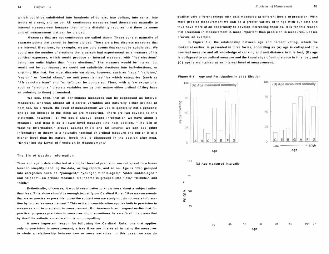
64 Chapter 5

w h i c h could be subdivided into hundreds of dol lars, into dollars, into cents, into

tenths of a cent, and so on. A l l continuous measures lend themselves naturally to

interval measurement because their infinite divisibi l i ty requires that there be some

unit of measurement that can be divided.

Measures that are not continuous are cal led discrete. These consist naturally of

separate points that cannot be further divided. There are a few discrete measures that

are interval. E lect ions, for example, are periodic events that cannot be subdivided. We

could use the number of elections that a person had experienced as a measure of his

polit ical exposure, wh ich would produce an interval measure, with "five elect ions"

being two units higher than "three elections." T h e measure would be interval but

would not be continuous; we could not subdivide elections into half-elections, or

anything l ike that. F o r most discrete variables, however, such as "race," "religion,"

"region," or "socia l c lass ," no unit presents itself by wh ich categories (such as

"A f r i can -Amer ican" and "white") can be compared. T h u s , with a few exceptions,

such as "elections," discrete variables are by their nature either ordinal (if they have

an ordering to them) or nominal .

We see, then, that al l cont inuous measures can be expressed as interval

measures , whereas a lmost al l d iscrete var iables are natural ly either ordinal or

nomina l . As a result , the level of measurement we use is general ly not a persona l

cho ice but inheres in the thing we are measur ing . T h e r e are two caveats to this

statement, however: (1) We cou ld a l w a y s ignore informat ion we have about a

measure , and treat i t as a lower - leve l measure (the next sect ion, " T h e S i n of

Wast ing Informat ion," argues against th is ) ; and (2) sometimes we can add other

information or theory to a natural ly nomina l or ordinal measure and enr ich it to a

higher level than its natural leve l : this is d i s c u s s e d in the sect ion after next,

" E n r i c h i n g the L e v e l o f P r e c i s i o n in Measurement ."

T h e S in o f W a s t i n g I n f o r m a t i o n

T i m e and again data col lected at a higher level of precision are col lapsed to a lower

level to simpli fy handling the data, writ ing reports, and so on. A g e is often grouped

into categories such as "youngest," "younger middle-aged," "older middle-aged,"

and "o ldes t "—an ordinal measure. Or income is grouped into "low," "middle," and

"high."

Esthetically, of course, it would seem better to know more about a subject rather

than less. Th is alone should be enough to justify our Cardinal Rule: " U s e measurements

that are as precise as possible, given the subject you are studying; do not waste informa­

tion by imprecise measurement." Th is esthetic consideration applies both to precision in

measures and to precision in measurement. But inasmuch as I argued earlier that for

practical purposes precision in measures might sometimes be sacrificed, it appears that

by itself the esthetic consideration is not compell ing.

A more important reason for fol lowing the Card ina l R u l e , one that applies

only to precis ion in measurement, arises if we are interested in using the measures

to study a relationship between two or more variables. In this case , we can do

Problems of Measurement 65

qualitatively different things wi th data measured at different levels of precis ion. Wi th

more precise measurement we can do a greater variety of things with our data and

thus have more of an opportunity to develop interesting theories. It is for this reason

that precision in measurement is more important than precis ion in measures. L e t me

provide an example.

In F igure 5 - 4 , the relationship between age and percent voting, w h i c h we

looked at earlier, is presented in three forms, according as ( A ) age is col lapsed to a

nominal measure and all knowledge of ranking and unit distance in it is lost; ( B ) age

is col lapsed to an ordinal measure and the knowledge of unit distance in it is lost; and

( C ) age is maintained at an interval level of measurement.

Figure 5 -4 Age and Participation in 2 0 0 2 Election

100 100

Low High

Age Age

100

75

c

•£ 50 CD O CD Q.

25

(C) Age measured intervally

30 40 50 60

Age

70 80 90 94

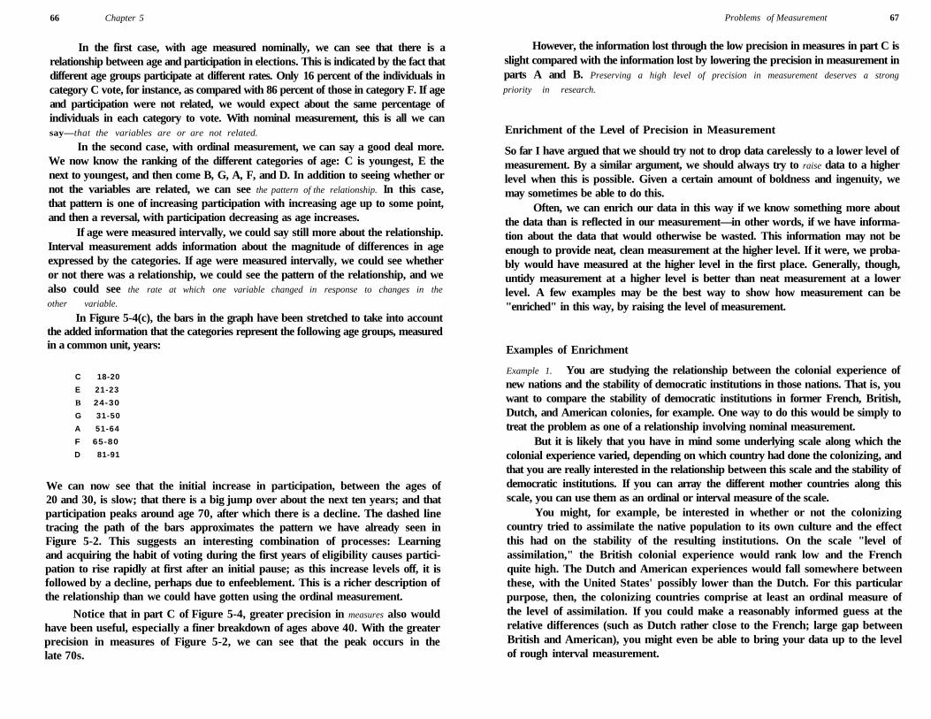
66 Chapter 5

In the first case, with age measured nominally, we can see that there is a relationship between age and participation in elections. This is indicated by the fact that different age groups participate at different rates. Only 16 percent of the individuals in category C vote, for instance, as compared with 86 percent of those in category F. If age and participation were not related, we would expect about the same percentage of individuals in each category to vote. With nominal measurement, this is all we can say—that the variables are or are not related.

In the second case, with ordinal measurement, we can say a good deal more. We now know the ranking of the different categories of age: C is youngest, E the next to youngest, and then come B, G, A, F, and D. In addition to seeing whether or not the variables are related, we can see the pattern of the relationship. In this case, that pattern is one of increasing participation with increasing age up to some point, and then a reversal, with participation decreasing as age increases.

If age were measured intervally, we could say still more about the relationship. Interval measurement adds information about the magnitude of differences in age expressed by the categories. If age were measured intervally, we could see whether or not there was a relationship, we could see the pattern of the relationship, and we also could see the rate at which one variable changed in response to changes in the

other variable.

In Figure 5-4(c), the bars in the graph have been stretched to take into account the added information that the categories represent the following age groups, measured in a common unit, years:

C 18-20

E 21-23

B 24-30

G 31-50

A 51-64

F 65-80

D 81-91

We can now see that the initial increase in participation, between the ages of 20 and 30, is slow; that there is a big jump over about the next ten years; and that participation peaks around age 70, after which there is a decline. The dashed line tracing the path of the bars approximates the pattern we have already seen in Figure 5-2. This suggests an interesting combination of processes: Learning and acquiring the habit of voting during the first years of eligibility causes partici­pation to rise rapidly at first after an initial pause; as this increase levels off, it is followed by a decline, perhaps due to enfeeblement. This is a richer description of the relationship than we could have gotten using the ordinal measurement.

Notice that in part C of Figure 5-4, greater precision in measures also would have been useful, especially a finer breakdown of ages above 40. With the greater precision in measures of Figure 5-2, we can see that the peak occurs in the late 70s.

Problems of Measurement 67

However, the information lost through the low precision in measures in part C is slight compared with the information lost by lowering the precision in measurement in parts A and B. Preserving a high level of precision in measurement deserves a strong

priority in research.

Enrichment of the Level of Precision in Measurement

So far I have argued that we should try not to drop data carelessly to a lower level of measurement. By a similar argument, we should always try to raise data to a higher level when this is possible. Given a certain amount of boldness and ingenuity, we may sometimes be able to do this.

Often, we can enrich our data in this way if we know something more about the data than is reflected in our measurement—in other words, if we have informa­tion about the data that would otherwise be wasted. This information may not be enough to provide neat, clean measurement at the higher level. If it were, we proba­bly would have measured at the higher level in the first place. Generally, though, untidy measurement at a higher level is better than neat measurement at a lower level. A few examples may be the best way to show how measurement can be "enriched" in this way, by raising the level of measurement.

Examples of Enrichment

Example 1. You are studying the relationship between the colonial experience of new nations and the stability of democratic institutions in those nations. That is, you want to compare the stability of democratic institutions in former French, British, Dutch, and American colonies, for example. One way to do this would be simply to treat the problem as one of a relationship involving nominal measurement.

But it is likely that you have in mind some underlying scale along which the colonial experience varied, depending on which country had done the colonizing, and that you are really interested in the relationship between this scale and the stability of democratic institutions. If you can array the different mother countries along this scale, you can use them as an ordinal or interval measure of the scale.

You might, for example, be interested in whether or not the colonizing country tried to assimilate the native population to its own culture and the effect this had on the stability of the resulting institutions. On the scale "level of assimilation," the British colonial experience would rank low and the French quite high. The Dutch and American experiences would fall somewhere between these, with the United States' possibly lower than the Dutch. For this particular purpose, then, the colonizing countries comprise at least an ordinal measure of the level of assimilation. If you could make a reasonably informed guess at the relative differences (such as Dutch rather close to the French; large gap between British and American), you might even be able to bring your data up to the level of rough interval measurement.

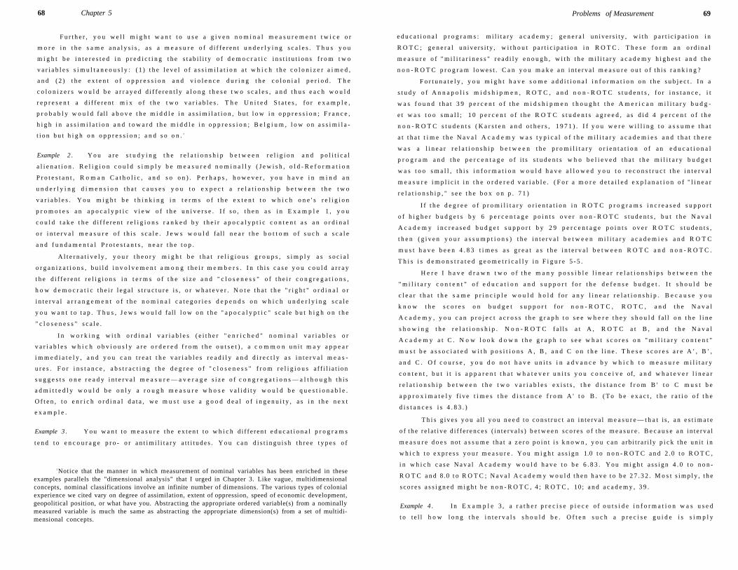
68 Chapter 5

F u r t h e r , y o u w e l l m i g h t w a n t t o u s e a g i v e n n o m i n a l m e a s u r e m e n t t w i c e o r

m o r e i n t h e s a m e a n a l y s i s , a s a m e a s u r e o f d i f f e r e n t u n d e r l y i n g s c a l e s . T h u s y o u

m i g h t b e i n t e r e s t e d i n p r e d i c t i n g t h e s t a b i l i t y o f d e m o c r a t i c i n s t i t u t i o n s f r o m t w o

v a r i a b l e s s i m u l t a n e o u s l y : ( 1 ) t h e l e v e l o f a s s i m i l a t i o n a t w h i c h t h e c o l o n i z e r a i m e d ,

a n d ( 2 ) t h e e x t e n t o f o p p r e s s i o n a n d v i o l e n c e d u r i n g t h e c o l o n i a l p e r i o d . T h e

c o l o n i z e r s w o u l d b e a r r a y e d d i f f e r e n t l y a l o n g t h e s e t w o s c a l e s , a n d t h u s e a c h w o u l d

r e p r e s e n t a d i f f e r e n t m i x o f t h e t w o v a r i a b l e s . T h e U n i t e d S t a t e s , f o r e x a m p l e ,

p r o b a b l y w o u l d fa l l a b o v e t h e m i d d l e i n a s s i m i l a t i o n , b u t l o w i n o p p r e s s i o n ; F r a n c e ,

h i g h i n a s s i m i l a t i o n a n d t o w a r d t h e m i d d l e i n o p p r e s s i o n ; B e l g i u m , l o w o n a s s i m i l a ­

t i o n b u t h i g h o n o p p r e s s i o n ; a n d s o o n . 5

Example 2 . Y o u a r e s t u d y i n g t h e r e l a t i o n s h i p b e t w e e n r e l i g i o n a n d p o l i t i c a l

a l i e n a t i o n . R e l i g i o n c o u l d s i m p l y b e m e a s u r e d n o m i n a l l y ( J e w i s h , o l d - R e f o r m a t i o n

P r o t e s t a n t , R o m a n C a t h o l i c , a n d s o o n ) . P e r h a p s , h o w e v e r , y o u h a v e i n m i n d a n

u n d e r l y i n g d i m e n s i o n t h a t c a u s e s y o u t o e x p e c t a r e l a t i o n s h i p b e t w e e n t h e t w o

v a r i a b l e s . Y o u m i g h t b e t h i n k i n g i n t e r m s o f t h e e x t e n t t o w h i c h o n e ' s r e l i g i o n

p r o m o t e s a n a p o c a l y p t i c v i e w o f t h e u n i v e r s e . I f s o , t h e n a s i n E x a m p l e 1 , y o u

c o u l d t a k e t h e d i f f e r e n t r e l i g i o n s r a n k e d b y t h e i r a p o c a l y p t i c c o n t e n t a s a n o r d i n a l

o r i n t e r v a l m e a s u r e o f t h i s s c a l e . J e w s w o u l d fa l l n e a r t h e b o t t o m o f s u c h a s c a l e

a n d f u n d a m e n t a l P r o t e s t a n t s , n e a r t h e t o p .

A l t e r n a t i v e l y , y o u r t h e o r y m i g h t b e t h a t r e l i g i o u s g r o u p s , s i m p l y a s s o c i a l

o r g a n i z a t i o n s , b u i l d i n v o l v e m e n t a m o n g t h e i r m e m b e r s . I n t h i s c a s e y o u c o u l d a r r a y

t h e d i f f e r e n t r e l i g i o n s i n t e r m s o f t h e s i z e a n d " c l o s e n e s s " o f t h e i r c o n g r e g a t i o n s ,

h o w d e m o c r a t i c t h e i r l e g a l s t r u c t u r e i s , o r w h a t e v e r . N o t e t h a t t h e " r i g h t " o r d i n a l o r

i n t e r v a l a r r a n g e m e n t o f t h e n o m i n a l c a t e g o r i e s d e p e n d s o n w h i c h u n d e r l y i n g s c a l e

y o u w a n t t o t a p . T h u s , J e w s w o u l d fa l l l o w o n t h e " a p o c a l y p t i c " s c a l e b u t h i g h o n t h e

" c l o s e n e s s " s c a l e .

I n w o r k i n g w i t h o r d i n a l v a r i a b l e s ( e i t h e r " e n r i c h e d " n o m i n a l v a r i a b l e s o r

v a r i a b l e s w h i c h o b v i o u s l y a r e o r d e r e d f r o m t h e o u t s e t ) , a c o m m o n u n i t m a y a p p e a r

i m m e d i a t e l y , a n d y o u c a n t r e a t t h e v a r i a b l e s r e a d i l y a n d d i r e c t l y a s i n t e r v a l m e a s ­

u r e s . F o r i n s t a n c e , a b s t r a c t i n g t h e d e g r e e o f " c l o s e n e s s " f r o m r e l i g i o u s a f f i l i a t i o n

s u g g e s t s o n e r e a d y i n t e r v a l m e a s u r e — a v e r a g e s i z e o f c o n g r e g a t i o n s — a l t h o u g h t h i s

a d m i t t e d l y w o u l d b e o n l y a r o u g h m e a s u r e w h o s e v a l i d i t y w o u l d b e q u e s t i o n a b l e .

O f t e n , t o e n r i c h o r d i n a l d a t a , w e m u s t u s e a g o o d d e a l o f i n g e n u i t y , a s i n t h e n e x t

e x a m p l e .

Example 3 . Y o u w a n t t o m e a s u r e t h e e x t e n t t o w h i c h d i f f e r en t e d u c a t i o n a l p r o g r a m s

t e n d t o e n c o u r a g e p r o - o r a n t i m i l i t a r y a t t i t u d e s . Y o u c a n d i s t i n g u i s h t h r e e t y p e s o f

5Notice that the manner in which measurement of nominal variables has been enriched in these examples parallels the "dimensional analysis" that I urged in Chapter 3. Like vague, multidimensional concepts, nominal classifications involve an infinite number of dimensions. The various types of colonial experience we cited vary on degree of assimilation, extent of oppression, speed of economic development, geopolitical position, or what have you. Abstracting the appropriate ordered variable(s) from a nominally measured variable is much the same as abstracting the appropriate dimension(s) from a set of multidi­mensional concepts.

Problems of Measurement 69

e d u c a t i o n a l p r o g r a m s : m i l i t a r y a c a d e m y ; g e n e r a l u n i v e r s i t y , w i t h p a r t i c i p a t i o n i n

R O T C ; g e n e r a l u n i v e r s i t y , w i t h o u t p a r t i c i p a t i o n i n R O T C . T h e s e f o r m a n o r d i n a l

m e a s u r e o f " m i l i t a r i n e s s " r e a d i l y e n o u g h , w i t h t h e m i l i t a r y a c a d e m y h i g h e s t a n d t h e

n o n - R O T C p r o g r a m l o w e s t . C a n y o u m a k e a n i n t e r v a l m e a s u r e o u t o f t h i s r a n k i n g ?

F o r t u n a t e l y , y o u m i g h t h a v e s o m e a d d i t i o n a l i n f o r m a t i o n o n t h e s u b j e c t . I n a

s t u d y o f A n n a p o l i s m i d s h i p m e n , R O T C , a n d n o n - R O T C s t u d e n t s , f o r i n s t a n c e , i t

w a s f o u n d t h a t 3 9 p e r c e n t o f t h e m i d s h i p m e n t h o u g h t t h e A m e r i c a n m i l i t a r y b u d g ­

e t w a s t o o s m a l l ; 1 0 p e r c e n t o f t h e R O T C s t u d e n t s a g r e e d , a s d i d 4 p e r c e n t o f t h e

n o n - R O T C s t u d e n t s ( K a r s t e n a n d o t h e r s , 1 9 7 1 ) . I f y o u w e r e w i l l i n g t o a s s u m e t h a t

a t t h a t t i m e t h e N a v a l A c a d e m y w a s t y p i c a l o f t h e m i l i t a r y a c a d e m i e s a n d t h a t t h e r e

w a s a l i n e a r r e l a t i o n s h i p b e t w e e n t h e p r o m i l i t a r y o r i e n t a t i o n o f a n e d u c a t i o n a l

p r o g r a m a n d t h e p e r c e n t a g e o f i t s s t u d e n t s w h o b e l i e v e d t h a t t h e m i l i t a r y b u d g e t

w a s t o o s m a l l , t h i s i n f o r m a t i o n w o u l d h a v e a l l o w e d y o u t o r e c o n s t r u c t t h e i n t e r v a l

m e a s u r e i m p l i c i t i n t h e o r d e r e d v a r i a b l e . ( F o r a m o r e d e t a i l e d e x p l a n a t i o n o f " l i n e a r

r e l a t i o n s h i p , " s e e t h e b o x o n p . 7 1 )

I f t h e d e g r e e o f p r o m i l i t a r y o r i e n t a t i o n i n R O T C p r o g r a m s i n c r e a s e d s u p p o r t

o f h i g h e r b u d g e t s b y 6 p e r c e n t a g e p o i n t s o v e r n o n - R O T C s t u d e n t s , b u t t h e N a v a l

A c a d e m y i n c r e a s e d b u d g e t s u p p o r t b y 2 9 p e r c e n t a g e p o i n t s o v e r R O T C s t u d e n t s ,

t h e n ( g i v e n y o u r a s s u m p t i o n s ) t h e i n t e r v a l b e t w e e n m i l i t a r y a c a d e m i e s a n d R O T C

m u s t h a v e b e e n 4 . 8 3 t i m e s a s g r e a t a s t h e i n t e r v a l b e t w e e n R O T C a n d n o n - R O T C .

T h i s i s d e m o n s t r a t e d g e o m e t r i c a l l y i n F i g u r e 5 - 5 .

H e r e I h a v e d r a w n t w o o f t h e m a n y p o s s i b l e l i n e a r r e l a t i o n s h i p s b e t w e e n t h e

" m i l i t a r y c o n t e n t " o f e d u c a t i o n a n d s u p p o r t f o r t h e d e f e n s e b u d g e t . I t s h o u l d b e

c l e a r t h a t t h e s a m e p r i n c i p l e w o u l d h o l d f o r a n y l i n e a r r e l a t i o n s h i p . B e c a u s e y o u

k n o w t h e s c o r e s o n b u d g e t s u p p o r t f o r n o n - R O T C , R O T C , a n d t h e N a v a l

A c a d e m y , y o u c a n p r o j e c t a c r o s s t h e g r a p h t o s e e w h e r e t h e y s h o u l d fa l l o n t h e l i n e

s h o w i n g t h e r e l a t i o n s h i p . N o n - R O T C f a l l s a t A , R O T C a t B , a n d t h e N a v a l

A c a d e m y a t C . N o w l o o k d o w n t h e g r a p h t o s e e w h a t s c o r e s o n " m i l i t a r y c o n t e n t "

m u s t b e a s s o c i a t e d w i t h p o s i t i o n s A , B , a n d C o n t h e l i n e . T h e s e s c o r e s a r e A ' , B ' ,

a n d C . O f c o u r s e , y o u d o n o t h a v e u n i t s i n a d v a n c e b y w h i c h t o m e a s u r e m i l i t a r y

c o n t e n t , b u t i t i s a p p a r e n t t h a t w h a t e v e r u n i t s y o u c o n c e i v e of, a n d w h a t e v e r l i n e a r

r e l a t i o n s h i p b e t w e e n t h e t w o v a r i a b l e s e x i s t s , t h e d i s t a n c e f r o m B ' t o C m u s t b e

a p p r o x i m a t e l y f i v e t i m e s t h e d i s t a n c e f r o m A ' t o B . ( T o b e e x a c t , t h e r a t i o o f t h e

d i s t a n c e s i s 4 . 8 3 . )

T h i s g i v e s y o u a l l y o u n e e d t o c o n s t r u c t a n i n t e r v a l m e a s u r e — t h a t i s , a n e s t i m a t e

o f t h e r e l a t i v e d i f f e r e n c e s ( i n t e r v a l s ) b e t w e e n s c o r e s o f t h e m e a s u r e . B e c a u s e a n i n t e r v a l

m e a s u r e d o e s n o t a s s u m e t h a t a z e r o p o i n t i s k n o w n , y o u c a n a r b i t r a r i l y p i c k t h e u n i t i n

w h i c h t o e x p r e s s y o u r m e a s u r e . Y o u m i g h t a s s i g n 1.0 t o n o n - R O T C a n d 2 . 0 t o R O T C ,

i n w h i c h c a s e N a v a l A c a d e m y w o u l d h a v e t o b e 6 . 8 3 . Y o u m i g h t a s s i g n 4 . 0 t o n o n -

R O T C a n d 8 .0 t o R O T C ; N a v a l A c a d e m y w o u l d t h e n h a v e t o b e 2 7 . 3 2 . M o s t s i m p l y , t h e

s c o r e s a s s i g n e d m i g h t b e n o n - R O T C , 4 ; R O T C , 10 ; a n d a c a d e m y , 3 9 .

Example 4 . I n E x a m p l e 3 , a r a t h e r p r e c i s e p i e c e o f o u t s i d e i n f o r m a t i o n w a s u s e d

t o t e l l h o w l o n g t h e i n t e r v a l s s h o u l d b e . O f t e n s u c h a p r e c i s e g u i d e i s s i m p l y

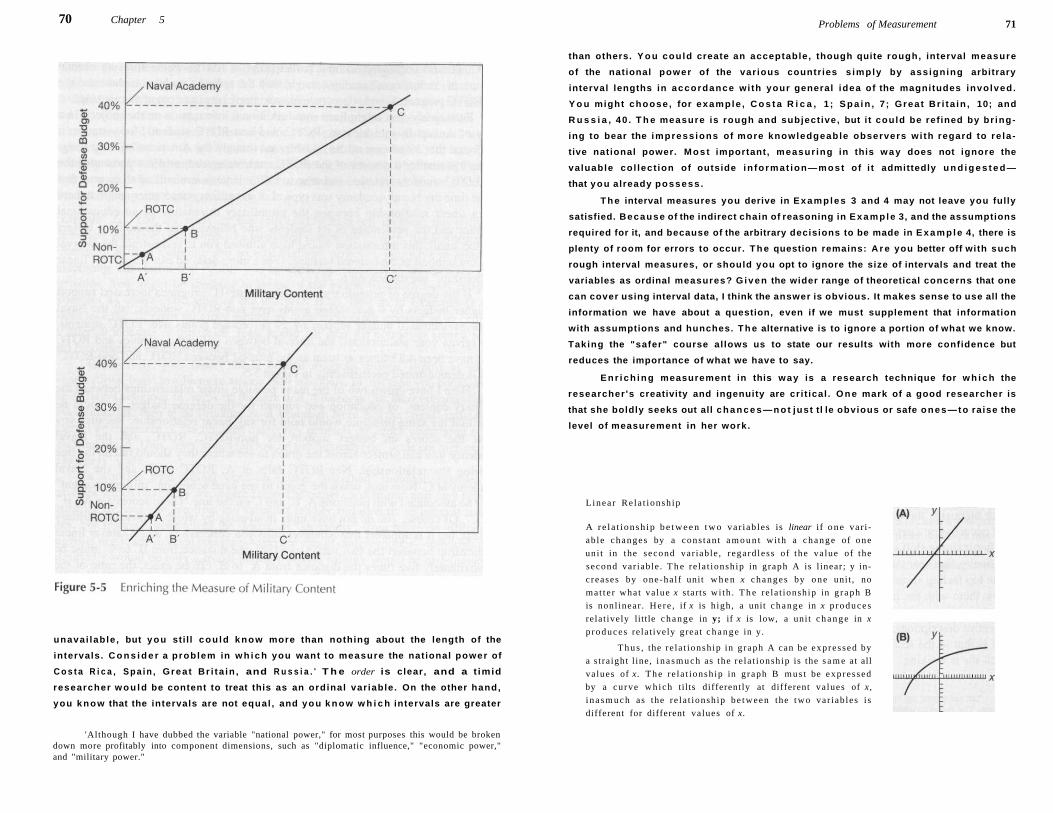
70 Chapter 5

unavai lable , but you sti l l cou ld know more than nothing about the length of the

intervals. C o n s i d e r a problem in w h i c h you want to measure the national power of

C o s t a R i c a , S p a i n , Great Br i ta in , and R u s s i a . 6 T h e order is clear, and a t imid

researcher w o u l d be content to treat this as an ordinal var iable. On the other hand,

you know that the intervals are not equal , and you k n o w w h i c h intervals are greater

'Although I have dubbed the variable "national power," for most purposes this would be broken down more profitably into component dimensions, such as "diplomatic influence," "economic power," and "military power."

Problems of Measurement 71

than others. Y o u could create an acceptable, though quite rough, interval measure

of the national power of the var ious countries s imply by ass igning arbitrary

interval lengths in accordance wi th your general idea of the magnitudes involved.

Y o u might choose , for example , C o s t a R i c a , 1 ; S p a i n , 7 ; Great Br i ta in , 10; and

R u s s i a , 40 . T h e measure is rough and subject ive, but i t could be ref ined by br ing­

ing to bear the impress ions of more knowledgeable observers wi th regard to re la ­

tive national power. M o s t important, measur ing in this w a y does not ignore the

valuable col lect ion of outside in format ion—most of i t admittedly u n d i g e s t e d —

that you already possess .

T h e interval measures you derive in Examples 3 and 4 may not leave you fully

satisfied. Because of the indirect chain of reasoning in E x a m p l e 3, and the assumptions

required for it, and because of the arbitrary decisions to be made in E x a m p l e 4, there is

plenty of room for errors to occur. T h e question remains: A r e you better off with such

rough interval measures, or should you opt to ignore the size of intervals and treat the

variables as ordinal measures? G iven the wider range of theoretical concerns that one

can cover using interval data, I think the answer is obvious. It makes sense to use all the

information we have about a question, even if we must supplement that information

with assumptions and hunches. T h e alternative is to ignore a portion of what we know.

Taking the "safer" course al lows us to state our results with more confidence but

reduces the importance of what we have to say.

E n r i c h i n g measurement in this way is a research technique for w h i c h the

researcher 's creativity and ingenuity are cr i t ical . O n e mark of a good researcher is

that she boldly seeks out all c h a n c e s — n o t just tl le obvious or safe ones—to raise the

level of measurement in her work.

Linea r Re la t ionsh ip

A re la t ionsh ip b e t w e e n t w o var iables is linear if one vari­

ab le changes by a cons tan t a m o u n t wi th a c h a n g e of one

uni t in the second var iable , regard less of the va lue of the

second var iable . T h e re la t ionship in graph A is l inear; y in­

c reases by one-ha l f unit w h e n x changes by one unit , no

mat te r wha t va lue x starts wi th . T h e re la t ionship in g raph B

is nonl inear . He re , if x is h igh , a unit c h a n g e in x p roduces

relat ively little c h a n g e in y; if x is low, a uni t c h a n g e in x

produces relat ively great c h a n g e in y.

T h u s , the re la t ionsh ip in g raph A can be expressed by

a s t ra ight l ine, i n a s m u c h as the re la t ionship is the s a m e at all

va lues of x. T h e re la t ionsh ip in g raph B mus t be expressed

by a cu rve wh ich tilts differently at different va lues of x,

i n a s m u c h as the re la t ionsh ip be tween the t w o var iab les i s

different for different va lues of x.

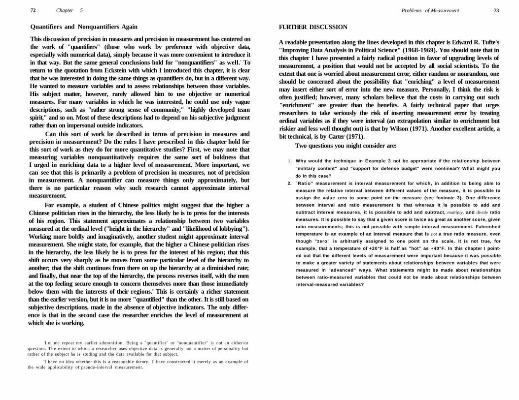
72 Chapter 5

Quantifiers and Nonquantifiers Again

This discussion of precision in measures and precision in measurement has centered on the work of "quantifiers" (those who work by preference with objective data, especially with numerical data), simply because it was more convenient to introduce it in that way. But the same general conclusions hold for "nonquantifiers" as well.7 To return to the quotation from Eckstein with which I introduced this chapter, it is clear that he was interested in doing the same things as quantifiers do, but in a different way. He wanted to measure variables and to assess relationships between those variables. His subject matter, however, rarely allowed him to use objective or numerical measures. For many variables in which he was interested, he could use only vague descriptions, such as "rather strong sense of community," "highly developed team spirit," and so on. Most of these descriptions had to depend on his subjective judgment rather than on impersonal outside indicators.

Can this sort of work be described in terms of precision in measures and precision in measurement? Do the rules I have prescribed in this chapter hold for this sort of work as they do for more quantitative studies? First, we may note that measuring variables nonquantitatively requires the same sort of boldness that I urged in enriching data to a higher level of measurement. More important, we can see that this is primarily a problem of precision in measures, not of precision in measurement. A nonquantifier can measure things only approximately, but there is no particular reason why such research cannot approximate interval measurement.

For example, a student of Chinese politics might suggest that the higher a Chinese politician rises in the hierarchy, the less likely he is to press for the interests of his region. This statement approximates a relationship between two variables measured at the ordinal level ("height in the hierarchy" and "likelihood of lobbying"). Working more boldly and imaginatively, another student might approximate interval measurement. She might state, for example, that the higher a Chinese politician rises in the hierarchy, the less likely he is to press for the interest of his region; that this shift occurs very sharply as he moves from some particular level of the hierarchy to another; that the shift continues from there on up the hierarchy at a diminished rate; and finally, that near the top of the hierarchy, the process reverses itself, with the men at the top feeling secure enough to concern themselves more than those immediately below them with the interests of their regions.8 This is certainly a richer statement than the earlier version, but it is no more "quantified" than the other. It is still based on subjective descriptions, made in the absence of objective indicators. The only differ­ence is that in the second case the researcher enriches the level of measurement at which she is working.

7 Let me repeat my earlier admonition. Being a "quantifier" or "nonquantifier" is not an either/or question. The extent to which a researcher uses objective data is generally not a matter of personality but rather of the subject he is studing and the data available for that subject.

8I have no idea whether this is a reasonable theory. I have constructed it merely as an example of the wide applicability of pseudo-interval measurement.

Problems of Measurement 73

FURTHER DISCUSSION

A readable presentation along the lines developed in this chapter is Edward R. Tufte's "Improving Data Analysis in Political Science" (1968-1969). You should note that in this chapter I have presented a fairly radical position in favor of upgrading levels of measurement, a position that would not be accepted by all social scientists. To the extent that one is worried about measurement error, either random or nonrandom, one should be concerned about the possibility that "enriching" a level of measurement may insert either sort of error into the new measure. Personally, I think the risk is often justified; however, many scholars believe that the costs in carrying out such "enrichment" are greater than the benefits. A fairly technical paper that urges researchers to take seriously the risk of inserting measurement error by treating ordinal variables as if they were interval (an extrapolation similar to enrichment but riskier and less well thought out) is that by Wilson (1971). Another excellent article, a bit technical, is by Carter (1971).

Two questions you might consider are:

1. Why would the technique in Example 3 not be appropriate if the relationship between

"military content" and "support for defense budget" were nonlinear? What might you

do in this case?

2. "Ratio" measurement is interval measurement for which, in addition to being able to

measure the relative interval between different values of the measure, it is possible to

assign the value zero to some point on the measure (see footnote 3). One difference

between interval and ratio measurement is that whereas it is possible to add and

subtract interval measures, it is possible to add and subtract, multiply, and divide ratio

measures. It is possible to say that a given score is twice as great as another score, given

ratio measurements; this is not possible with simple interval measurement. Fahrenheit

temperature is an example of an interval measure that is not a true ratio measure, even

though "zero" is arbitrarily assigned to one point on the scale. It is not true, for

example, that a temperature of +20°F is half as "hot" as +40°F. In this chapter I point­

ed out that the different levels of measurement were important because it was possible

to make a greater variety of statements about relationships between variables that were

measured in "advanced" ways. What statements might be made about relationships

between ratio-measured variables that could not be made about relationships between

interval-measured variables?

Chapter 6

QoJ)

T h u s far everything we have looked at in this book has been just i f ied in terms of how

useful it is in establishing relationships between variables. It is time now to look

more c losely at what a "relat ionship" is , and how we interpret it.

T w o variables are related if certain values of one variable tend to coincide with

certain values of the other variable. T h u s , socia l c lass and party vote are related in

the Uni ted States, because those w h o vote Republ ican tend to be from the middle

and upper c lasses . We have seen many such examples of relationships in earlier

chapters.

If, in addit ion, we cons ider that the values of one var iable produce the

va lues of the other var iable , the relat ionship is a causal relationship. T h e example

of c l a s s and vot ing, noted above, is an example of a causa l re lat ionship. We feel

that there is something about a person 's s o c i a l c l a s s that makes that person

more l ike ly to vote in a certain way. There fore , we say that soc ia l c l a s s is a

" c a u s e " of party vote. I t is not mere ly true that the two var iables tend to co inc ide ;

they tend to co inc ide because values of the one tend to produce distinct values of

the other.

E m p i r i c a l , theory-oriented polit ical research is almost exclusively concerned

with causal relationships. As I pointed out earlier, a theory in its simplest form

usual ly consists of three things: independent variables (those we think of as doing

the "producing") , dependent variables (those we think of as being "produced") , and

causal statements l inking the two (refer again to p. 14).

In this chapter we first d iscuss the idea of causat ion, and then fol low this

up with some ideas on research design. Research des ign—the way in w h i c h we

structure the gathering of data—strongly affects the conf idence with w h i c h we can

put a causal interpretation on the results of research.

74

Causal Thinking and Design of Research 75

C A U S A L I T Y : A N I N T E R P R E T A T I O N

T h e most important thing to note about causa l thinking is that it is an interpretation

of reality. In this regard, the assert ion of a causal relationship differs f rom the mere

assert ion of a relationship, w h i c h is a rather objective statement. In the example of

social c lass and the vote, for instance, there is objective evidence for the existence

of a relat ionship, but a causa l interpretation of this relationship is m u c h more

subject ive. It might be argued, for instance, that c lass does not produce the vote, but

that both are produced by something e lse—the ethnic, re l igious, and rac ia l conf l icts

that have surfaced often in A m e r i c a n pol i t ics. T h u s someone could a r g u e — a n d it

would not be an unreasonable argument—that c lass is not a cause of the vote.

Rather, that person might say, certain ethnic groups tend to vote for the Democra ts ;

and these same groups, s imply by accident, also tend to be work ing c lass .

Therefore , the co inc idence of c lass and party votes is just that—a coinc idence.

D is t inguishing between this version of the relat ionship and the more c o m m o n

version is at least partly a matter of judgment.

A lmost every situation in w h i c h we w i s h to make causal statements is similar to

this example. The question of whether or not there is a relationship is objectively

testable. T h e question of whether the relationship is a causal one, and of wh ich variable

causes wh ich , requires an interpretation. General ly speaking, all that we know directly

from our data is that two variables tend to occur together. To read causality into such

co-occurrence, we must add something more, although as you wi l l see, it is possible to

design the research in ways that can help us significantly in doing this.

Cons ider two further examples: I f we see that people who smoke regularly

have a greater incidence of heart disease than nonsmokers, we might conclude that

smoking causes heart disease. I f we see that those U . S . senators who conform to the

informal rules of the Senate tend to be the ones whose bil ls get passed, we might

conclude that conformity is rewarded in the Senate. In both cases , we observe that

two phenomena tend to occur together (smoking and heart disease, conformity and

success ) . O u r interpretation of this is that one of the phenomena causes the other.

T h i s interpretation is a subjective one.

We cannot a lways make a causal interpretation when two phenomena tend to

coincide. T h e notion of cause involves more than that. Winter does not cause spring,

although the one fol lows the other regularly. S imi lar ly , hair color does not cause

polit ical party preference, although it is probably true in the Uni ted States that

blonds, who are relatively l ikely to be white and Protestant, are more apt than

brunettes to be Republ icans. To qualify as a " c a u s a l " relationship, the coinc idence of

two phenomena must include the idea that one of them produces the other.

A good example of the difficulty of ascribing causal direction is the relationship

between central bank independence and inflation. In general, economists think that if

central banks (such as the Federal Reserve in the United States) are relatively

independent of political control, they wi l l use monetary policy more aggressively to

fight inflation. Certainly, where central banks are independent, inflation is low. In a

76 Chapter 6

1993 study, the three countries with the most politicized banks had averaged almost 8 percent inflation from 1955 to 1985; the three countries whose central banks were most independent had averaged only about 3.75 percent inflation.'

We see, then, that there is a relationship between the two; but is it true, as the economists believe, that bank independence causes low inflation? Batalla (1993) suggests that the opposite causal interpretation may be true. Reviewing the history of the 1920s and 1930s in Latin America, he notes that many countries had established autonomous central banks by the late 1920s, but that when high rates of inflation hit in the mid-1930s, most of them took away that autonomy. That is, low inflation rates allowed governments to tolerate independent central banks, while high inflation rates led the governments to pull the banks under their control. So, which causes which? Do independent central banks give us low inflation, or does low inflation give us independent central banks?

If ascribing cause to the coincidence of two things is so tricky, why do we bother with the notion of causation in our theories? What difference does it make whether class causes voting for a certain party, or whether the coincidence of class and party is due to something else that causes both of them? Remember that the ultimate purpose of theories is to give us levers on reality, some basis for choosing how to act. If A and B coincide but A does not cause B, changing A will not change B. Coincidence without cause gives you no lever.

ELIMINATION OF ALTERNATIVE CAUSAL INTERPRETATIONS

A causal interpretation is something that cannot come solely from our observations. But by setting up a study in certain ways and by manipulating the data appropriately, we can settle some of the problems in making causal interpretations. In our previous example of hair color, for instance, we might have looked only at WASPs, and compared blonds and brunettes. If we then found that blond WASPs did not tend more often than brunette WASPs to be Republican, we could infer that hair color did not cause party preference.

In general, where we think that a third variable is causing two other vari­ables to coincide accidentally, as in this hair color example, we can use our data to test the relationship. By holding constant the third variable, we can see whether it has led the original two variables to coincide in such a way as to resemble a causal relationship. Thus, if we artificially hold social position constant by look­ing only at WASPs, and now blonds and brunettes no longer differ in their politics, we can infer that the difference in voting was due not to the difference in hair color (which was merely a coincident variable) but to the difference in socioethnic background. We can then conclude that hair color does not cause political preference.2

'The Economist, November 20. 1993, p. 94. 2 The technique of holding constant is discussed in greater detail at the conclusion of the chapter.

Causal Thinking and Design of Research 77

Thus there are techniques by which we can manipulate our data to eliminate some of the alternative causal interpretations of a relationship. But there is always one question about causation that remains purely subjective and that cannot be resolved completely by any techniques of data handling. Given that two variables are causally related, which of the variables causes which?

Suppose that two phenomena coincide and that there appears to be a causal relationship between them. Only you can decide which is the cause and which, the result. One useful convention in Western culture—but it is only a convention, even though it is so well established that it seems "natural" to us—is that causation works forward in time.3 Accordingly, if we can establish that change in one of the variables precedes change in the other, and if we are sure that there is causation between the two, it is clear which variable must be the cause. For example, we assume that pulling a trigger causes the shot that follows, rather than vice versa.

Although this convention frequently simplifies things for the researcher, there are many instances in which it cannot be used. Survey research, in which variables usually are measured just once and in a single interview, is a case in point. If voters who like the Republican party also tend to oppose welfare programs, which causes which? We might think that voters choose the party that offers the policies they prefer, but it might also be that voters choose the Republican party for other reasons, such as foreign policy, and then are influenced by the party's leaders to adopt its position on welfare programs as their own.

Summary

Let me pull together the argument to this point. It generally is not enough for us to note that two phenomena coincide. We generally also want to interpret why they coincide. There are three interpretations available to us, and our choice from among them is ultimately subjective.

/. Causation is not involved at all. The phenomena coincide because of logical necessity; that is, their coincidence is tautologically determined. Thus, by definition, spring follows winter, yet we do not think of winter as producing spring. A slight variation of this often occurs in the social sciences. It often happens that two slightly different measures of the same concept coincide. We would expect them to coincide, simply because they measure the same thing; we do not think of either of them as causing the other. For example, members of Congress who vote to increase aid to education tend also to support increases in welfare spending. This is not because their votes on one issue cause them to vote the way they do on the other. Rather, both votes are an expression of their general disposition to spend money on social programs. We must decide from outside the data at hand whether a coincidence of two phenomena is of this type or whether it involves causation.

3 An example of a cultural tradition in which causation does not necessarily work forward in time is that of the Old Testament, whose writers believed that some people could prophesy what was to come in the future. In effect, the future event caused the prior prophecy to occur.

78 Chapter 6

2. The relationship we observe is a result of outside factors that cause the two phenomena at hand, and thus neither of these phenomena causes the other. The study of hair color and party preference was an example of this. By setting up the study appropriately, we can control for various outside factors in order to concentrate on the relationship in question. In the hair color example, such a control was used. To this extent, we can see from the data whether the coincidence of the phenomena is of this sort. But we are still not exempt from making assumptions, for we must first have assumed the outside factor(s) causally prior to the two coincident phenomena. This is not always an easy decision to make. If it is possible to set up a true experiment (described in the next section), we can eliminate this possibility. But this is often not possible in "field" social sciences such as political science or sociology.

3. One of the phenomena causes the other. Here we have a true causal statement. We are still not finished making assumptions, of course, for we must decide which of the phenomena is the cause and which the effect. That is ultimately a subjective decision, though often we are aided in making it by the convention that causation must run forward in time.

As I have said so often in this book, one of the pleasures of research is that nothing in it is automatic. Even the most "quantitative" techniques do not take away our obligation and our right to be creative and imaginative. The fact that causal analy­sis is ultimately subjective may trouble us—objectivity always seems more comfort­ing than the responsibility imposed by subjective judgment—but in a way it is also a great comfort, inasmuch as it keeps us, and what we do with our minds, at the heart of our research.

A FEW BASICS OF RESEARCH DESIGN

It should be evident from the discussion so far that the basic problem in causal analysis is that of eliminating alternative causal interpretations. Whenever two variables vary together (are related, coincide), there is a variety of causal sequences that might account for their doing so. A might cause B, B might cause A, both A and B might be caused by something else, or there might be no causation involved. Our task is to eliminate all but one of these, thus leaving an observed relationship, together with a single causal interpretation of it. Some of these alternatives can be eliminated only if we make assumptions from outside the actual study. But we also can design the study in such a way that certain alternatives are impossible. This will leave an interpretation that is dependent on fewer subjective assumptions and can thus lend a greater measure of certainty to the results.

Consider these examples:

/. Agency study. An organizational analysis of a government agency is made in which workers keep track of their output for a week. The organization is then restructured to

Causal Thinking and Design of Research 79

decentralize decision making. After the reform, another week's tabulation shows increased output. Conclusion: Decentralized decision making increases output.

2. Reagan's victory over the Soviet Union. During the Reagan administration (1980-1988) the United States steadily increased its military spending. Over the three years from 1989 to 1991 the Soviet Union collapsed, which conservatives hailed as a victory for Reagan's policies. Conclusion: The economic strain of matching Reagan's military buildup had been too much for the Soviet system, and had led to its collapse and the end of the Cold War.

3. Organizing the poor. In anticipation of a major campaign to organize the poor of a city, a survey is taken among them to measure their interest in politics. At the end of the organizing campaign, the same people are asked the same questions a second time. It turns out that those who were contacted by the campaign workers have indeed acquired an increased interest in politics, compared with those who were not. Conclusion: The campaign has increased the political awareness of the poor.

4. Tax-reform mail. The Congressional Quarterly reports the proportion of each senator's mail which favored tax reform. Comparing these figures with the senators' votes on a tax-reform bill, we see that senators who had received relatively favorable mail tended to vote for the bill, whereas those who had received relatively unfavorable mail tended to vote against it. Conclusion: How favorable a senator's mail was on tax reform affected whether or not she voted for it.

5. Presidential lobbying. In an attempt to measure his influence over Congress, the president randomly selects half the members of the House. He conducts a straw vote to find out how all the members of the House intend to vote on a bill important to him. He then lobbies intensively among the half he has randomly selected. In the final vote in the House, the group that he had lobbied shifted in his favor compared with what he could have expected from the earlier straw vote; the other half voted as predicted from the straw vote. Conclusion: His lobbying helped the bill.

Let us look at the design of these studies to see how many alternative causal interpretations each can eliminate.

Designs Without a Control Group

In the first two examples, the design is of the form:

1. M e a s u r e the d e p e n d e n t var iable .

2 . O b s e r v e that the i ndependen t var iable occurs .

3 . M e a s u r e the dependen t var iab le again.

4 . I f the d e p e n d e n t var iab le has changed , ascr ibe that to the occur rence of the i ndependen t

var iable .

80 Chapter 6

T h u s , i n " A g e n c y S t u d y , " ( 1 ) t h e w o r k e r s ' o u t p u t i s t a b u l a t e d ; ( 2 ) t h e o r g a n i ­

z a t i o n a l s t r u c t u r e i s d e c e n t r a l i z e d ; ( 3 ) t h e w o r k e r s ' o u t p u t i s o n c e a g a i n t a b u l a t e d ;

a n d ( 4 ) t h e c o n c l u s i o n i s r e a c h e d . T h i s k i n d o f d e s i g n o p e r a t e s without a control

group. A s a r e s u l t , t h e r e a r e a n u m b e r o f a l t e r n a t i v e c a u s a l s e q u e n c e s t h a t m i g h t h a v e

p r o d u c e d t h e s a m e r e s u l t .

F o r e x a m p l e , a p l a u s i b l e a l t e r n a t i v e e x p l a n a t i o n f o r t h e i n c r e a s e d p r o d u c t i v i t y

m i g h t b e t h a t t h e i n i t i a l m e a s u r e m e n t o f p r o d u c t i o n , i n w h i c h e a c h w o r k e r k e p t t r a c k

o f o u t p u t f o r a w e e k , f o c u s e d t h e w o r k e r s ' a t t e n t i o n o n p r o d u c t i v i t y i n a w a y t h a t h a d

n o t b e e n d o n e b e f o r e , l e a d i n g t h e m t o i m p r o v e t h e i r p r o d u c t i v i t y . I n o t h e r w o r d s ,

i t w a s n o t t h e d e c e n t r a l i z a t i o n o f t h e a g e n c y , b u t t h e s t u d y i tself , w h i c h c a u s e d

p r o d u c t i v i t y t o r i s e . 4

H a d t h e s t u d y i n c l u d e d a s e c o n d a g e n c y a s a c o n t r o l ( s e e t h e n e x t s e c t i o n ) , o n e i n

w h i c h o u t p u t w a s m e a s u r e d a t t h e s a m e t i m e s a s i n t h e f irs t a g e n c y b u t i n w h i c h t h e r e

w a s n o d e c e n t r a l i z a t i o n , t h e a l t e r n a t i v e e x p l a n a t i o n w o u l d n o t h a v e b e e n p l a u s i b l e .

T h a t i s , i f t h e i n c r e a s e d p r o d u c t i v i t y i n " A g e n c y S t u d y " h a d b e e n d u e s i m p l y t o t h e ac t

o f m e a s u r i n g , p r o d u c t i v i t y i n t h e c o n t r o l a g e n c y ( in w h i c h t h e s a m e m e a s u r e m e n t s

w e r e t a k e n a s i n t h e f irs t a g e n c y ) a l s o s h o u l d h a v e i n c r e a s e d . A c c o r d i n g l y , i f w e f o u n d

t h a t p r o d u c t i v i t y i n c r e a s e d m o r e i n t h e r e o r g a n i z e d a g e n c y t h a n i n t h e c o n t r o l a g e n c y ,

w e w o u l d k n o w t h a t t h i s c o u l d n o t h a v e b e e n b e c a u s e o f t h e ac t o f m e a s u r i n g , fo r

b o t h a g e n c i e s w o u l d h a v e u n d e r g o n e t h e s a m e m e a s u r e m e n t s . T h a t p a r t i c u l a r

a l t e r n a t i v e i n t e r p r e t a t i o n w o u l d h a v e b e e n e l i m i n a t e d b y t h e d e s i g n o f t h e s t u d y . I n

c o n d u c t i n g t h e s t u d y w i t h o u t a c o n t r o l , t h e a l t e r n a t i v e i n t e r p r e t a t i o n c a n b e e l i m i n a t e d

o n l y b y a s s u m i n g i t a w a y , w h i c h s e e m s v e r y r i sky .

" R e a g a n ' s v i c t o r y o v e r t h e S o v i e t U n i o n " p r o v i d e s a n e x a m p l e o f a n o t h e r

s o r t o f a l t e r n a t i v e e x p l a n a t i o n t h a t m a y b e p l a u s i b l e i n s t u d i e s w i t h o u t a c o n t r o l

g r o u p . I t i s q u i t e p o s s i b l e t h a t o t h e r t h i n g s t h a t o c c u r r e d b e t w e e n t h e m e a s u r e ­

m e n t o f t h e t w o e v e n t s ( 1 9 8 0 - 1 9 8 8 a n d 1 9 8 9 - 1 9 9 1 ) w e r e t h e c a u s e o f t h e S o v i e t

U n i o n ' s c o l l a p s e . R e f o r m i n C o m m u n i s t C h i n a , t h e g r o w t h o f M u s l i m m i n o r i t i e s

i n t h e S o v i e t U n i o n , f e u d s a m o n g S o v i e t l e a d e r s — a l l m i g h t b e p r o p o s e d a s

a l t e r n a t i v e c a u s e s o f t h e S o v i e t U n i o n ' s c o l l a p s e . I f i t w e r e p o s s i b l e t o f i n d a s a

c o n t r o l g r o u p a s i m i l a r s y s t e m t h a t w e n t t h r o u g h t h e s a m e o t h e r f a c t o r s b u t w a s

n o t e n g a g e d i n a n a r m s r a c e w i t h t h e U n i t e d S t a t e s , t h e n t h e s e a l t e r n a t i v e

e x p l a n a t i o n s c o u l d b e t e s t e d a n d p e r h a p s e l i m i n a t e d . B u t o f c o u r s e , n o s u c h

s y s t e m e x i s t s .

T h i s i s a g o o d e x a m p l e o f h o w d i f f i c u l t i t m a y s o m e t i m e s b e t o i n c l u d e a

c o n t r o l g r o u p i n a d e s i g n . S o m e c i r c u m s t a n c e s j u s t d o n o t y i e l d p a r a l l e l c a s e s t h a t

c a n b e c o m p a r e d . A s a n o t h e r e x a m p l e , c o n s i d e r t h a t t h e e x i s t e n c e o f t h e U n i t e d

4A famous example of this sort is the Hawthorne study, in which an attempt was made to measure how much productivity increased when factories were made brighter and more pleasant. As it turned out, the groups of workers who were placed in better surroundings did show major increases in productivity. But so did control groups whose surroundings had not been improved. The novelty of taking part in an experiment, the attention paid to the workers, and increased social cohesiveness among those groups chosen for the experiment—all these raised productivity irrespective of the experimental changes in physical working conditions that were made for some (but not all) of the groups. See Roethlisberger and Dickson (1939).

Causal Thinking and Design of Research 81

N a t i o n s h a s a f f e c t e d t h e f o r e i g n p o l i c y o f e v e r y c o u n t r y i n t h e w o r l d s i n c e 1 9 4 5 .

H o w c a n a s t u d e n t o f i n t e r n a t i o n a l p o l i t i c s d i s t i n g u i s h i t s e f f e c t o n f o r e i g n p o l i c y

f r o m t h e e f f e c t s o f t h e S o v i e t - A m e r i c a n r i v a l r y , t h e d e v e l o p m e n t o f a t o m i c

w e a p o n s , t h e l i b e r a t i o n o f f o r m e r c o l o n i e s , a n d s o o n , a l l o f w h i c h h a v e h a p p e n e d

a t t h e s a m e t i m e ? O n e c a n n o t , o f c o u r s e . I t i s s i m p l y n o t p o s s i b l e t o p r o v i d e a

c o n t r o l g r o u p o f c o n t e m p o r a r y c o u n t r i e s f o r w h i c h t h e U n i t e d N a t i o n s h a s n o t

e x i s t e d .

T h e s a m e g e n e r a l a l t e r n a t i v e e x p l a n a t i o n ( t h a t o t h e r t h i n g s h a p p e n i n g a t t h e

s a m e t i m e c o u l d h a v e b e e n t h e t r u e c a u s e ) a l s o m i g h t h a v e a p p l i e d t o " A g e n c y

S t u d y . " I f s o m e t h i n g e l s e h a d h a p p e n e d b e t w e e n t h e t w o m e a s u r e m e n t s o f

p r o d u c t i v i t y — t h e w e a t h e r i m p r o v e d , C h r i s t m a s c a m e , t h e p r e s i d e n t u r g e d g r e a t e r

p r o d u c t i v i t y , o r w h a t e v e r — t h i s m i g h t h a v e b e e n t h e t r u e c a u s e o f t h e i n c r e a s e d

p r o d u c t i o n . A g a i n , u s i n g a s e c o n d a g e n c y a s a c o n t r o l c o u l d e l i m i n a t e s u c h a l t e r n a ­

t i v e e x p l a n a t i o n s .

S t u d i e s w i t h o u t a c o n t r o l g r o u p p o p u p al l t h e t i m e . O n J a n u a r y 4 , 2 0 0 4 , t h e

Minneapolis Star Tribune h e a d l i n e d a f r o n t - p a g e s t o r y : " S t a t e S e x Ed N o t W o r k i n g ,

S t u d y F i n d s . " T h e s t o r y r e p o r t e d a s t u d y b y t h e M i n n e s o t a D e p a r t m e n t o f H e a l t h ,

w h i c h i n 2 0 0 1 h a d a s k e d s t u d e n t s i n g r a d e s 7 a n d 8 o f t h r e e s c h o o l s t h a t h a d a d o p t e d

a n a b s t i n e n c e - o n l y s e x e d u c a t i o n c u r r i c u l u m ( n o t t e a c h i n g c o n t r a c e p t i o n o r s a f e s e x ,

b u t r a t h e r p r o v i d i n g m a t e r i a l s t o e n c o u r a g e s t u d e n t s t o a b s t a i n ) , w h e t h e r " a t a n y t i m e

i n y o u r l i fe h a v e y o u e v e r h a d s e x ( i n t e r c o u r s e ) ? " T h e y t h e n c a m e b a c k i n 2 0 0 2 a n d

r e p e a t e d t h e q u e s t i o n fo r t h e s a m e g r o u p o f s t u d e n t s , n o w i n g r a d e s 8 a n d 9 . F r o m

2 0 0 1 t o 2 0 0 2 t h e n u m b e r s a y i n g t h a t t h e y h a d e v e r h a d s e x u a l i n t e r c o u r s e r o s e f r o m

5 .8 t o 1 2 . 4 p e r c e n t . T h e c o n c l u s i o n o f t h e a r t i c l e w a s t h a t t h e a b s t i n e n c e - o n l y

c u r r i c u l u m h a d f a i l ed .

A n a b s t i n e n c e - o n l y c u r r i c u l u m m i g h t o r m i g h t n o t fa i l t o r e d u c e s e x u a l

i n t e r c o u r s e , b u t w e c a n n o t t e l l f r o m t h i s s t u d y w h i c h i s t h e c a s e . S t u d e n t s o f t h a t

a g e , a s t h e y g r o w a y e a r o l d e r , a r e i n a n y c a s e p r o b a b l y m o r e l i k e l y t o h a v e s e x u a l

i n t e r c o u r s e t h a n w h e n t h e y w e r e y o u n g e r . A c o n t r o l g r o u p o f s t u d e n t s o f t h e s a m e

a g e w h o h a d h a d a d i f f e r e n t c u r r i c u l u m f o r s e x e d u c a t i o n w o u l d h a v e b e e n e a s y t o

a d d t o t h e s t u d y , b u t w i t h o u t i t w e h a v e n o i d e a w h e t h e r t h e s t u d e n t s w i t h t h e

a b s t i n e n c e - o n l y c u r r i c u l u m i n i t i a t e d s e x u a l a c t i v i t y a t a g r e a t e r r a t e t h a n t h e y

w o u l d h a v e d o n e w i t h o u t t h e c u r r i c u l u m , a t a l e s s e r r a t e , o r a t t h e s a m e r a t e . W e

s i m p l y c a n n o t t e l l w h e t h e r t h e a b s t i n e n c e - o n l y c u r r i c u l u m r e s u l t e d i n r e d u c e d

s e x u a l i n t e r c o u r s e .

( T h e p r o b l e m o f i n t e r p r e t i n g r e s u l t s w a s a l s o e x a c e r b a t e d i n t h i s c a s e b y t h e

q u e s t i o n , w h i c h a s k e d s t u d e n t s w h e t h e r a t a n y t i m e i n t h e i r l i f e t h e y h a d e v e r h a d

s e x u a l i n t e r c o u r s e . T h e 5 . 8 p e r c e n t w h o a n s w e r e d a f f i r m a t i v e l y i n 2 0 0 1 m u s t h a v e

a n s w e r e d a f f i r m a t i v e l y a g a i n i n 2 0 0 2 , s o t h e p e r c e n t r e s p o n d i n g " y e s " i n 2 0 0 2

c o u l d h a v e o n l y r i s e n o r s t a y e d t h e s a m e ; i t w a s n o t p o s s i b l e f o r t h e p e r c e n t a g e t o

d e c l i n e . S o , a p p a r e n t f a i l u r e o f t h e p r o g r a m w a s b a k e d i n t o t h e s t u d y f r o m t h e

s t a r t . A b e t t e r q u e s t i o n w o r d i n g , w h i c h w o u l d h a v e b e e n m o r e s e n s i t i v e t o t h e

i m p a c t o f t h e n e w p r o g r a m , w o u l d h a v e b e e n : " D u r i n g t h e p a s t y e a r , h a v e y o u h a d

s e x [ i n t e r c o u r s e ] ? " )

82 Chapter 6

U s e o f a C o n t r o l G r o u p

The natural experiment. "Organiz ing the Poor" is an example of a design in

w h i c h a control group has been added to handle the sorts of problems we just

encountered. It is a natural experiment, a design in w h i c h a test group (that is , a

group exposed to the independent variable) and a control group (a group not exposed

to the independent variable) are used, but in w h i c h the investigator has no control

over w h o falls into the test group and who falls into the control group. In

"Organiz ing the Poor," the matter of w h o was contacted by the campaign workers

was decided by the workers ' own choice of w h o m to contact and by the extent

to w h i c h different people made themselves available for contact by the campaign

workers. T h e natural experiment design is of the form:

1. Measure the dependent variable for a specific population before it is exposed to the

independent variable.

2. Wait until some among the population have been exposed to the independent variable.

3. Measure the dependent variable again.

4. If between measurings the group that was exposed (called the test group) has changed

relative to the control group, ascribe this to the effect of the independent variable on the

dependent variable.

T h u s , in "Organiz ing the Poor," (1) a number of poor people were surveyed as

to their interest in pol i t ics; (2) the campaign occurred; (3) the same poor people were

surveyed again; and (4) those who had been contacted by the campaign were

compared with those who had not. T h i s design el iminates many of the alternative

explanations that can crop up in work ing without a control group. F o r instance, it

could not have been the init ial measurement that changed the group that had

been contacted, compared wi th the control group, because both groups had been

measured in the same way.

Never the less , the natural exper iment st i l l a l lows alternative explanat ions.

B e c a u s e the researcher does not have control over w h o is exposed to the

independent var iable , it may be that the exposed group has a different pred ispos i ­

t ion to change than the control group. In " O r g a n i z i n g the Poor," for instance, the

campa ign workers are l ike ly to have approached those poor w h o m they thought

they c o u l d most eas i ly get interested in pol i t ics . A l s o , those among the poor w h o

were most resistant to change might not have let the campa ign workers in the

door or might have been chron ica l l y absent w h e n the campa ign workers tr ied to

contact them. A c c o r d i n g l y , a p laus ib le alternative explanat ion in " O r g a n i z i n g the

P o o r " is that the poor w h o were contacted by the campaign increased their

interest in pol i t ics more than those w h o were not contacted simply because they were the ones who showed more potential to become more interested in politics at that time, regardless of the campaign. T h i s alternative must be either a s s u m e d

away or control led by us ing a des ign in w h i c h the researcher can determine w h o

fal ls into the test group and w h o fal ls into the control group. A des ign that

Causal Thinking and Design of Research 83

a c c o m p l i s h e s this is a true experiment; but before going on to d i s c u s s this, let me

d i s c u s s a poor cous in of the natural exper iment .

The natural experiment without premeasurement. T h i s is a design in w h i c h no

measurements are made before subjects are exposed to the independent variable.

Th is design fol lows the form:

1. Measure the dependent variable for subjects, some of whom have been exposed to the

independent variable (the test group) and some of whom have not (the control group).

2. If the dependent variable differs between the groups, ascribe this to the effect of the

independent variable.

T h e " T a x - R e f o r m M a i l " example is of this sort. In this design, (1) senators'

votes on a tax-reform bi l l were noted, and (2) the votes of senators w h o had

received favorable mai l were compared wi th the votes of those who had not. T h e

same k ind of alternative explanation that has to be dealt wi th in natural experiments

has to be dealt wi th in this design also. As in "Organ iz ing the Poor," i t m a y be that

heavier pro- tax - re form ma i l went to senators w h o already were moving into a tax-

reform posit ion even without the mai l . S u c h senators, about w h o m there might have

been a great deal of speculat ion in the press, could have attracted more mai l than

did other senators.

Moreover , this design permits many addit ional alternative explanat ions

beyond those that apply to a natural experiment. In the tax-reform example , it is

probable that people were more l ike ly to write 1 ;tters favoring re form to senators

they thought w o u l d agree wi th them. In other words , i t might be that senators ' ma i l

did not cause their votes, but that their l ike ly vote c a u s e d them to get certain k inds

of ma i l . H e n c e , the relat ionship between a senator 's vote on the bi l l and the ma i l

she rece ived might not be a causat ive relat ionship at a l l — m e r e l y a co inc idence

between pro-reform and pro -ma i l and ant i -reform and ant i -mai l . T h i s alternative

could not apply to a natural experiment. In a natural experiment it wou ld have been

clear f rom the init ial measurement whether or not those w h o fell into the test group

had ini t ia l ly been different f rom those fal l ing into the control group. In fact, what

is compared in the natural exper iment is not the measured variables themselves ,

but how the two groups change between measurements .

To s u m up, the natural exper iment without premeasurement is a des ign in

w h i c h the test group and the control group are c o m p a r e d wi th respect to a de­

pendent var iable only after they have been exposed to the independent var iable . I t

involves the same sorts of alternative explanat ions as the natural exper iment does,

plus some others that result f rom the fact that the investigator does not k n o w what

the test group and the control group looked l ike before the whole thing started.

T rue E x p e r i m e n t

In neither of the two versions of the natural experiment just outlined did the investi­

gator have any control over who fell into the test group and who fell into the control

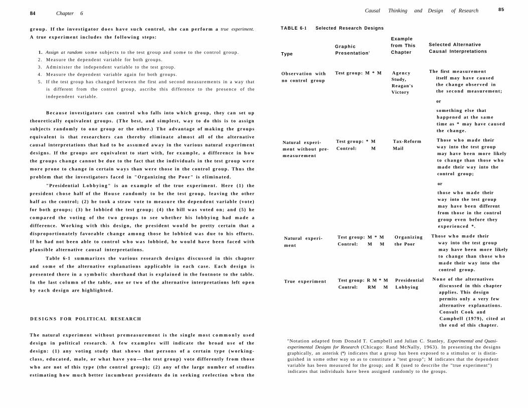
84 Chapter 6

g r o u p . I f the i n v e s t i g a t o r d o e s h a v e s u c h c o n t r o l , s h e c a n p e r f o r m a true experiment.

A true e x p e r i m e n t i n c l u d e s the f o l l o w i n g s t eps :

1. Assign at random s o m e subjects to the test g roup and s o m e to the control g r o u p .

2 . M e a s u r e the d e p e n d e n t var iable for both g roups .

3 . A d m i n i s t e r the independen t var iable to the test g r o u p .

4 . M e a s u r e the dependen t var iable again for both g roups .

5. If the test g roup has c h a n g e d be tween the first and second m e a s u r e m e n t s in a way that

is different from the control g roup , ascr ibe this difference to the p r e sence of the

i ndependen t var iable .

B e c a u s e i n v e s t i g a t o r s c a n contro l w h o fa l l s i n t o w h i c h g r o u p , t h e y c a n set u p

t h e o r e t i c a l l y e q u i v a l e n t g r o u p s . ( T h e bes t , a n d s i m p l e s t , w a y t o d o this i s t o a s s i g n

s u b j e c t s r a n d o m l y t o o n e g r o u p o r the other . ) T h e a d v a n t a g e o f m a k i n g the g r o u p s

e q u i v a l e n t i s that r e s e a r c h e r s c a n t h e r e b y e l i m i n a t e a l m o s t all o f the a l t ernat ive

c a u s a l in terpreta t ions that h a d t o b e a s s u m e d a w a y i n the v a r i o u s natural e x p e r i m e n t

d e s i g n s . I f the g r o u p s are e q u i v a l e n t to start w i t h , for e x a m p l e , a d i f f e r e n c e in h o w

the g r o u p s c h a n g e c a n n o t b e d u e t o the fact that the i n d i v i d u a l s i n the test g r o u p w e r e

m o r e p r o n e t o c h a n g e i n cer ta in w a y s than w e r e t h o s e i n the contro l g r o u p . T h u s the

p r o b l e m that the i n v e s t i g a t o r s f a c e d in " O r g a n i z i n g the P o o r " i s e l i m i n a t e d .

"Pres ident ia l L o b b y i n g " i s a n e x a m p l e o f the true e x p e r i m e n t . H e r e ( 1 ) the

p r e s i d e n t c h o s e ha l f o f the H o u s e r a n d o m l y t o b e the tes t g r o u p , l e a v i n g the o ther

h a l f a s the c o n t r o l ; ( 2 ) h e t o o k a s traw v o t e t o m e a s u r e the d e p e n d e n t v a r i a b l e ( v o t e )

for b o t h g r o u p s ; ( 3 ) h e l o b b i e d the test g r o u p ; ( 4 ) the bi l l w a s v o t e d o n ; a n d ( 5 ) h e

c o m p a r e d t h e v o t i n g o f the t w o g r o u p s t o s e e w h e t h e r h i s l o b b y i n g had m a d e a

d i f f e r e n c e . W o r k i n g w i t h th i s d e s i g n , the p r e s i d e n t w o u l d be pretty cer ta in that a

d i s p r o p o r t i o n a t e l y f a v o r a b l e c h a n g e a m o n g t h o s e h e l o b b i e d w a s d u e t o h i s e f forts .

I f h e h a d n o t b e e n a b l e t o c o n t r o l w h o w a s l o b b i e d , h e w o u l d h a v e b e e n f a c e d w i t h

p l a u s i b l e a l ternat ive c a u s a l in terpreta t ions .

T a b l e 6 -1 s u m m a r i z e s the v a r i o u s r e s e a r c h d e s i g n s d i s c u s s e d i n this c h a p t e r

and s o m e o f the a l t ernat ive e x p l a n a t i o n s a p p l i c a b l e i n e a c h c a s e . E a c h d e s i g n i s

p r e s e n t e d there in a s y m b o l i c s h o r t h a n d that i s e x p l a i n e d in the f o o t n o t e to the tab le .

I n the last c o l u m n o f the tab le , o n e o r t w o o f the a l t ernat ive in terpreta t ions left o p e n

b y e a c h d e s i g n are h i g h l i g h t e d .

D E S I G N S F O R P O L I T I C A L R E S E A R C H

T h e natural e x p e r i m e n t w i t h o u t p r e m e a s u r e m e n t i s the s i n g l e m o s t c o m m o n l y u s e d

d e s i g n i n p o l i t i c a l r e s e a r c h . A f e w e x a m p l e s w i l l i n d i c a t e the b r o a d u s e o f the

d e s i g n : ( 1 ) a n y v o t i n g s t u d y that s h o w s that p e r s o n s o f a cer ta in t y p e ( w o r k i n g -

c l a s s , e d u c a t e d , m a l e , o r w h a t h a v e y o u — t h e tes t g r o u p ) v o t e d i f f e r e n t l y f r o m t h o s e

w h o are no t o f th i s t y p e ( t h e c o n t r o l g r o u p ) ; ( 2 ) a n y o f t h e large n u m b e r o f s t u d i e s

e s t i m a t i n g h o w m u c h be t ter i n c u m b e n t p r e s i d e n t s d o i n s e e k i n g r e e l e c t i o n w h e n the

Causal Thinking and Design of Research 85

TABLE 6-1 Selected Research Designs

Type

Graphic Presentation 3

Example from This Chapter

Selected Alternative Causal Interpretations

O b s e r v a t i o n with

no control group

Test group: M * M A g e n c y Study, Reagan's Victory

Natural exper i ­m e n t w i t h o u t pre­m e a s u r e m e n t

Test group: * M Tax-Reform

Control: M Mail

Natural exper i ­

ment

True e x p e r i m e n t

Test group: M * M O r g a n i z i n g

Control: M M the Poor

Test group: R M * M Presidential

Control: RM M Lobbying

The first m e a s u r e m e n t itself may have c a u s e d the c h a n g e o b s e r v e d in the s e c o n d m e a s u r e m e n t ;

or

s o m e t h i n g e l s e that

h a p p e n e d a t the s a m e

t ime as * may have c a u s e d

the c h a n g e .

Those w h o m a d e their

w a y into the test g r o u p

may have b e e n m o r e likely

t o c h a n g e than t h o s e w h o

m a d e their w a y into the

control group;

or

t h o s e w h o m a d e their

w a y into the test group

may have b e e n different

from t h o s e in the control

group e v e n before they

e x p e r i e n c e d *.

T h o s e w h o m a d e their

w a y into the test g r o u p

may have b e e n m o r e likely

t o c h a n g e than t h o s e w h o

m a d e their w a y into the

control group .

N o n e o f the alternatives d i s c u s s e d in this chapter appl i e s . This d e s i g n permits o n l y a very f e w alternative e x p l a n a t i o n s . Consul t C o o k and C a m p b e l l ( 1 9 7 9 ) , c i ted at the e n d of this chapter.

"Notation adapted from Donald T. Campbell and Julian C. Stanley, Experimental and Quasi-experimental Designs for Research (Chicago: Rand McNally, 1963). In presenting the designs graphically, an asterisk (*) indicates that a group has been exposed to a stimulus or is distin­guished in some other way so as to constitute a "test group"; M indicates that the dependen t variable has been measured for the group; and R (used to describe the "true experiment") indicates that individuals have been assigned randomly to the groups.

86 Chapter 6

e c o n o m y h a s i m p r o v e d i n t h e p r e c e d i n g y e a r ( t e s t g r o u p ) c o m p a r e d w i t h t h o s e fo r

w h o m t h e e c o n o m y h a s n o t b e e n i m p r o v i n g ( c o n t r o l g r o u p ) ; ( 3 ) m o s t " p o l i c y

o u t p u t " s t u d i e s , s u c h a s o n e b y R o g o w s k i a n d K a y s e r ( 2 0 0 2 ) , w h i c h s h o w e d t h a t

m a j o r i t a r i a n e l e c t o r a l s y s t e m s ( t h e t e s t g r o u p ; a l s o k n o w n a s s i n g l e - m e m b e r

d i s t r i c t , p l u r a l i t y s y s t e m s , t h e k i n d o f s y s t e m u s e d i n U . S . H o u s e e l e c t i o n s a n d

B r i t i s h a n d C a n a d i a n e l e c t i o n s ) w i l l t e n d t o p r o d u c e e c o n o m i c p o l i c i e s f a v o r a b l e t o

c o n s u m e r s , w h i l e p r o p o r t i o n a l r e p r e s e n t a t i o n s y s t e m s ( t h e c o n t r o l g r o u p , e l e c t o r a l

s y s t e m s l i k e t h o s e o f G e r m a n y , S w e d e n , a n d t h e N e t h e r l a n d s ) s h o u l d s t r e n g t h e n t h e

i n t e r e s t s o f p r o d u c e r s ; a n d ( 4 ) s t u d i e s o f d i s c r i m i n a t i o n , s u c h a s U h l a n e r a n d

S c h l o z m a n ( 1 9 8 6 ) , w h o t e s t e d w h e t h e r w o m e n c a n d i d a t e s f o r o f f i c e w e r e l e s s w e l l

f i n a n c e d t h a n m e n b e c a u s e o f e x p e r i e n t i a l a t t r i b u t e s s u c h a s s e n i o r i t y , o r b e c a u s e o f

d i r e c t d i s c r i m i n a t i o n .

I n s h o r t , a n y r e s e a r c h i s a n e x a m p l e o f t h e n a t u r a l e x p e r i m e n t w i t h o u t

p r e m e a s u r e m e n t i f i t ( 1 ) t a k e s t w o o r m o r e t y p e s o f s u b j e c t s a n d c o m p a r e s t h e i r

v a l u e s o n a d e p e n d e n t v a r i a b l e ; a n d ( 2 ) i n f e r s t h a t t h e d i f f e r e n c e o n t h e d e p e n d e n t

v a r i a b l e i s t h e r e s u l t o f t h e i r d i f f e r e n c e o n w h a t e v e r i t i s t h a t d i s t i n g u i s h e s t h e m a s

" t y p e s . " 5 T h i s r e a l l y d e s c r i b e s t h e b u l k o f p o l i t i c a l r e s e a r c h .

A s w e s a w i n e a r l i e r s e c t i o n s , t h i s d e s i g n i s f a r f r o m s a t i s f a c t o r y . I t p e r m i t s

r e l a t i v e l y m a n y a l t e r n a t i v e c a u s a l i n t e r p r e t a t i o n s , w h i c h a r e d i f f i cu l t t o h a n d l e .

N e v e r t h e l e s s , t h i s r e m a i n s t h e m o s t w i d e l y u s e d d e s i g n i n p o l i t i c a l s c i e n c e . O t h e r

d e s i g n s t h a t h a v e t h e a d v a n t a g e o f c o n t r o l g r o u p s a r e t o b e p r e f e r r e d b e c a u s e t h e y

r e q u i r e l e s s d i f f i c u l t a s s u m p t i o n s , b u t t h e s e d e s i g n s c a n b e u s e d o n l y w h e n t h e

r e s e a r c h e r h a s m o r e c o n t r o l o v e r t h e t e s t v a r i a b l e s t h a n m o s t p o l i t i c a l s c i e n t i s t s c a n

u s u a l l y a c h i e v e .

I n o r d e r t o u s e a n a t u r a l e x p e r i m e n t d e s i g n , f o r i n s t a n c e , r e s e a r c h e r s m u s t b e

a b l e t o a n t i c i p a t e t h e o c c u r r e n c e o f t h e t e s t f a c t o r . T h e y a l s o m u s t g o t o t h e e x p e n s e

i n t i m e a n d m o n e y o f m a k i n g t w o m e a s u r e m e n t s o f t h e s u b j e c t s . E v e n t h e n , t h e

a t t e m p t m a y m i s f i r e ; f o r e x a m p l e , i t m a y b e t h a t t h e t e s t f a c t o r ( e s p e c i a l l y i f i t i s o n e

t h a t a f f e c t s o n l y a s m a l l p a r t o f t h e p o p u l a t i o n ) w i l l a p p l y t o o n l y a f e w o f t h e p e o p l e

i n c l u d e d i n t h e s t u d y . T h a t i s , t h e i n v e s t i g a t o r m a y b e l e f t w i t h a c o n t r o l g r o u p b u t n o

t e s t g r o u p .

M a n y i m p o r t a n t v a r i a b l e s i n t h e s o c i a l s c i e n c e s a r e n o t a t a l l s u s c e p t i b l e t o

s t u d y b y n a t u r a l e x p e r i m e n t s . S o m e l i e i n t h e p a s t : p e o p l e ' s e x p e r i e n c e s d u r i n g t h e

D e p r e s s i o n , t h e c o l o n i a l h i s t o r i e s o f n a t i o n s , t h e e d u c a t i o n a l b a c k g r o u n d s a n d p a s t

p r o f e s s i o n s o f m e m b e r s o f C o n g r e s s , a n d s o o n . O t h e r s , s u c h a s a s s a s s i n a t i o n s , r i o t s ,

a n d c h a n g e s i n t h e b u s i n e s s c y c l e , a r e u n p r e d i c t a b l e . S u c h v a r i a b l e s a r e d i f f i c u l t t o

5 I t is apparent here and in the examples directly preceding this that I am taking some liberty with the notion of "control group." Where rates of participation in the middle class and working class are compared, for instance, it is not at all clear which class is the "test" group and which is the "control." The distinction is even muddier when one compares several groups simultaneously, such as voters from several age groups. But the logic of what is done here is the same as in the strict test/control situation, where the dependent variable is compared among groups of subjects distinguished by their values on the independent variable. It is convenient and revealing to treat this sort of analysis in terms of the analogy to experiments.

Causal Thinking and Design of Research 87

fit i n t o a n a t u r a l e x p e r i m e n t d e s i g n . O n t h e o t h e r h a n d , s o m e e v e n t s a r e m o r e e a s i l y

a n t i c i p a t e d : t h e i n t r o d u c t i o n o f a p o v e r t y p r o g r a m i n a t o w n , h i g h s c h o o l g r a d u a t e s '

e n t r a n c e i n t o c o l l e g e , r e g u l a r l y s c h e d u l e d p o l i t i c a l e v e n t s s u c h a s e l e c t i o n s , a n d s o

o n . T h e s e l e n d t h e m s e l v e s r e a d i l y t o a n a t u r a l e x p e r i m e n t a l d e s i g n .

A t r u e e x p e r i m e n t r e q u i r e s e v e n g r e a t e r c o n t r o l o v e r t h e s u b j e c t s o f t h e s t u d y

t h a n d o e s a n a t u r a l e x p e r i m e n t . T h e l a t t e r r e q u i r e s o n l y t h a t t h e i n v e s t i g a t o r b e a b l e t o

a n t i c i p a t e e v e n t s , b u t t h e t r u e e x p e r i m e n t r e q u i r e s t h a t t h e r e s e a r c h e r b e a b l e t o

m a n i p u l a t e t h o s e e v e n t s — s h e m u s t d e c i d e w h o i s t o fa l l i n t o t h e c o n t r o l g r o u p a n d

w h o i s t o fa l l i n t o t h e e x p e r i m e n t a l g r o u p . T o d o t h i s i n a f i e ld s i t u a t i o n r e q u i r e s

p o w e r o v e r p e o p l e i n t h e i r n o r m a l l i v e s . T h u s i t i s n o a c c i d e n t t h a t t h e e x a m p l e I u s e d

o f a t r u e e x p e r i m e n t , " P r e s i d e n t i a l L o b b y i n g , " w a s c a r r i e d o u t b y t h e p r e s i d e n t . I t i s

r a r e i n r e a l p o l i t i c a l s i t u a t i o n s t h a t a r e s e a r c h e r c a n e x e r c i s e t h i s k i n d o f c o n t r o l o v e r

e v e n t s . H o w e v e r , t h e e x p e r i m e n t i s s o m u c h m o r e p o w e r f u l t h a n o t h e r d e s i g n s —

r e j e c t s a l t e r n a t i v e i n t e r p r e t a t i o n s s o d e c i s i v e l y — t h a t w e s h o u l d u s e i t w h e n e v e r

p o s s i b l e , a n d p r o b a b l y s h o u l d u s e i t a g o o d d e a l m o r e t h a n i s n o w d o n e . 6

A c h e n ( 1 9 8 6 , p . 6 ) , c i t i n g G i l b e r t , L i g h t , a n d M o s t e l l e r ( 1 9 7 5 ) , p o i n t s o u t t h a t

a p p a r e n t l y only r a n d o m i z a t i o n p r o v i d e s a c l e a r - e n o u g h c a u s a l i n t e r p r e t a t i o n t o s e t t l e

i s s u e s o f s o c i a l - s c i e n t i f i c r e s e a r c h c o n c l u s i v e l y :

Wi thou t it, even the c leveres t statistical analys is mee t s s t rong res i s tance f rom other

schola i s , w h o s e profess ional skept ic i sm is qui te natura l . W h e n the forces that deter­

m i n e the exper imen ta l and cont ro l g roups are u n k n o w n , the imag ina t ion has full p lay to

create al ternat ive exp lana t ions for the data . Invent ing hypo theses of this sort is enjoy­

able , uns t r enuous labor that i s rare ly resis ted.

I t m a y b e t h a t i n a s m a l l o r g a n i z a t i o n , s u c h a s a l o c a l p o l i t i c a l c a u c u s o r a

p o r t i o n o f a c a m p u s , t h e i n v e s t i g a t o r c a n c a r r y o u t a t r u e e x p e r i m e n t a l d e s i g n . F o r

i n s t a n c e , s t u d e n t s m i g h t c o n d u c t a p o l i t i c a l c a m p a i g n a m o n g a r a n d o m l y s e l e c t e d

p o r t i o n o f t h e c a m p u s c o m m u n i t y a n d c o m p a r e t h a t p o r t i o n o v e r t i m e w i t h a

r a n d o m l y s e l e c t e d c o n t r o l .

I t i s s o m e t i m e s p o s s i b l e t o c a r r y o u t t r u e e x p e r i m e n t s o n a l a r g e r s c a l e t h a n

t h i s , b u t o n l y i f t h e e x p e r i m e n t e r c a n c o n t r o l s i g n i f i c a n t p o l i c i e s a n d m a n i p u l a t e

t h e m f o r t h e p u r p o s e s o f i n v e s t i g a t i o n . A g o o d e x a m p l e o f t h i s s o r t o f e x p e r i m e n t i s

G e r b e r a n d G r e e n ( 2 0 0 0 ) , i n w h i c h 3 0 , 0 0 0 r e g i s t e r e d v o t e r s i n N e w H a v e n ,

C o n n e c t i c u t , w e r e e a c h r a n d o m l y a s s i g n e d o n e o f t h r e e d i f f e r e n t a p p r o a c h e s i n a

n o n p a r t i s a n g e t - o u t - t h e - v o t e p r o g r a m . I t t u r n e d o u t t h a t p e r s o n a l v i s i t s w e r e

e f f e c t i v e i n g e t t i n g p e o p l e t o v o t e , d i r e c t m a i l a p p e a l s h e l p e d s l i g h t l y , a n d t e l e p h o n e

c a l l s m a d e n o d i f f e r e n c e a t a l l .

A n o t h e r i n t e r e s t i n g e x a m p l e o f a n a t u r a l s i t u a t i o n t h a t p r o d u c e d s o m e t h i n g

a p p r o x i m a t i n g a t r u e e x p e r i m e n t i s t h e s t u d y b y H o w e l l e t a l . ( 2 0 0 2 ) o f t h e e f f e c t s o f

a p r i v a t e e d u c a t i o n o n p o o r c h i l d r e n . P r o g r a m s w e r e i n i t i a t e d i n D a y t o n , O h i o :

6Kinder and Palfrey (1993, especially the Introduction) argue persuasively that we in political science have overrated the problems and barriers to true experimentation in our field.

88 Chapter 6

Washington, D.C.; and New York City that offered children in public schools partial scholarship vouchers to attend private schools. Since there were more applicants than could be funded, children were chosen by lottery to receive the vouchers. This selection process approximated a true experiment; the scholarships were assigned randomly, and there was a control group of children who applied for scholarships but did not receive them. Thus, the two groups should have been equivalent in all respects other than the experimental treatment. The result of the study was that African American students who received the scholarships did significantly better on standardized tests two years later than African American students who did not receive the scholarships. No other ethnic group appeared to benefit in the same way.

This study comes very close to a true experiment, and therefore offers very convincing results on an important policy issue. One remaining alternative explana­tion is that something akin to the problem we saw in 'Agency Study" was operating. The children who received scholarships knew they had won something special. Also, they knew that their parents were paying extra money beyond the partial scholarship to further their education. This may have left them more highly motivated than the students who had not won in the lottery. (In an ideal experiment, people do not know whether they are in the experimental group or in the control; the New Haven study by Gerber and Green is an example.) This worry might be lessened, however, by the fact that it was only African Americans who appeared to benefit from the vouchers; if the benefit were an artifact of children's knowing they had won in the lottery, one would think that would affect all ethnic groups in the same way.

When it is possible to construct true (or nearly true) experiments in real field situations like this, the results can be compelling. More often, true experi­mentation is useful for studying general aspects of small-group interactions or individual thought processes relevant to politics. For example, a group of subjects may be placed together and told to reach a decision on some question. The investigator then manipulates the way individuals in the group may communicate with each other, to see how this influences the result. In such studies, of course, true experiments are the most appropriate design, inasmuch as the investigator generally can control all the relevant variables. A good example of this sort of experiment is that of Iyengar and Kinder (1987), in which the investigators tested experimentally the effects of variations in the format of TV news reporting on subjects' political perceptions.

Special Design Problem for Policy Analysis: Regression to the Mean

I have introduced you above to some simple sources of alternative causal interpretations and some simple designs to control for them. A slightly more complex problem, while it has many applications in general explanation, is especially important in evaluating the impact of policy initiatives. This is a problem most public officials and journalists do not appear to understand at all, but it is well within your range of understanding at this point.

Causal Thinking and Design of Research 89

The problem is called regression to the mean. If we assume that essentially everything we observe has some element of randomness to it—that is, in addition to its true core value it varies somewhat from time to time—regression to the mean will always be present. Consider a student in a course, for example. When she is tested, her measured level of knowledge is generally about right, but if she has had a bad day (isn't feeling good, has bad luck in the instructor's choice of questions, and so on), she will score somewhat below her usual level; on a good day, she will score somewhat higher. Note that this sort of random variation in a measure is closely related to what we referred to as unreliability in Chapter 4.

For our purposes here, the important thing about this is that if we observe cases at two points in time, we can expect high initial values to drop somewhat from one time to the next, and low initial values to rise somewhat. Not all of them will do this; some of the high scores no doubt are genuinely high and may even rise by the next time they are observed. But a disproportionate number of the high cases are probably cases for whom things had lined up unusually well the first time; that is, the random part of their measure is likely to have been positive. We should expect that it is unlikely they would be so lucky twice in a row, so on the average they are likely to go down the next time they are observed. Similarly, the lowest scores probably include a disproportionate number of cases that were unusually low because of a negative random factor; on the average, we should see them rise.

We should therefore be a little suspicious of a statement.like: "Team learning strategies are good in that the weakest students improve, but they are bad in that the strongest students appear to be dragged down by working with the weaker ones." This could be true. But an alternative explanation could be that this is simply regression to the mean. It might be that the stronger students' scores declined because when they were measured at the beginning of the experiment with team learning, a number of them had done unusually well and then just drifted back to their normal level of performance over time. Similarly, some of the poorer students might have drifted up to their normal levels. In other words, the scores of the weaker students might have improved, and the scores of the stronger students might have declined, even if the students had never been involved in team learning. The two alternative causal interpretations can only be sorted out by using an appropriate research design. (One is given on p. 90)

One variant of this problem shows up time and again in assessing the impact of new governmental policies. How often have you seen a statement of the sort: "After foot patrols were introduced in the entertainment district, our city's murder rate declined by a full 18 percent"? What is often missed in such statements is that this effect might also be due to regression to the mean. When do cities typically institute new policies? When the problem they are concerned about has flared up! But cities' problems, like students taking tests, probably have some element of randomness to their measures. If the murder rate has shot up in one year, it is more likely to go down the next year than to go still higher, whether or not the city institutes foot patrols in the entertainment district. In other words, governments are likely to pick a time when a problem is at a high point (which may or may not include some random element)

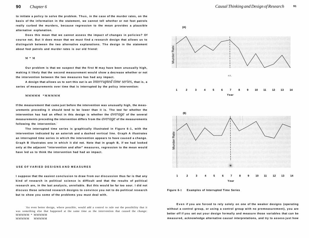
90 Chapter 6

to initiate a pol icy to solve the problem. T h u s , in the case of the murder rates, on the

basis of the information in the statement, we cannot tell whether or not foot patrols

really curbed the murders, because regression to the mean provides a plausible

alternative explanation.

D o e s this mean that we cannot assess the impact of changes in po l ic ies? Of

course not. But it does mean that we must f ind a research design that a l lows us to

dist inguish between the two alternative explanations. T h e design in the statement

about foot patrols and murder rates is our old friend:

M * M

O u r problem is that we suspect that the first M may have been unusual ly h igh,

making it l ikely that the second measurement would show a decrease whether or not

the intervention between the two measures has had any impact.

A design that a l lows us to sort this out is an interrupted time series, that is , a

series of measurements over time that is interrupted by the policy intervention:

M M M M M * M M M M M

If the measurement that came just before the intervention was unusually high, the meas­

urements preceding it should tend to be lower than it is. The test for whether the

intervention has had an effect in this design is whether the average of the several

measurements preceding the intervention differs from the average of the measurements

following the intervention. 7

T h e interrupted time series is graphical ly il lustrated in F igure 6 - 1 , with the

intervention indicated by an asterisk and a dashed vertical l ine. G r a p h A illustrates

an interrupted time series in w h i c h the intervention appears to have caused a change.

G r a p h B illustrates one in w h i c h it did not. Note that in graph B, if we had looked

only at the adjacent "intervention and after" measures, regression to the mean would

have led us to think the intervention had had an impact.

U S E O F V A R I E D D E S I G N S A N D M E A S U R E S

I suppose that the easiest conclus ion to draw f rom our d iscussion thus far is that any

k ind of research in polit ical sc ience is difficult and that the results of poli t ical

research are, in the last analys is , unreliable. But this would be far too sour. I did not

d iscuss these selected research designs to convince you not to do polit ical research

but to show you some of the problems you must deal with.

7 An even better design, where possible, would add a control to rule out the possibility that it was something else that happened at the same time as the intervention that caused the change: M M M M M * MMMMM M M M M M MMMMM

Causal Thinking and Design of Research 91

(A)

A l Z ,

1 2 3 4 5 6 7 8 9 10 11 12 13 14

Year

(B)

1 2 3 4 5 6 7 8 9 10 11 12 13 14

Year

Figure 6-1 Examples of Interrupted Time Series

E v e n if you are forced to rely solely on one of the weaker designs (operating

without a control group, or using a control group wi th no premeasurement) , you are

better off if you set out your design formally and measure those variables that can be

measured, acknowledge alternative causal interpretations, and try to assess just how

92 Chapter 6

likely it is that each alternative is true. The choice is between doing this or giving up and relying on your intuition and impressions.

But there is a more hopeful side to this chapter. The various weaknesses of different designs should suggest a solution: Wherever possible, try to work simultane­ously with a variety of designs, which can at least in part cancel out each other's weak­nesses. For example, in working solely with a randomized experiment in an isolated situation, we may wonder whether the result we have obtained might be a result of something about the way the experiment was set up, rather than a "true" result. Relying totally on a natural experiment, we might wonder whether our results simply reflect a test group comprised of unusual people, rather than a "true" result. But if we could use both of these designs, employing either the same or closely related measures, each result would bolster the other. We could be more confident of the experimental result if we had gotten a similar result in a field situation. And we could be more confident of the result of the natural experiment if we had gotten a similar result in an artificial true experiment.

If we can mix research strategies in this way, the end result is more than the sum of its parts. The strengths of the various designs complement each other. The likelihood that the alternative explanations associated with each design are true decreases because of the confirmation from the other design. It will seem less likely to us that the result of the natural experiment is due to unusual people entering the test group, for example, if we obtain similar results in a true experiment, whose test group we controlled.

Note that the effect would not be the same if a single research design were repeated twice—if, say, a natural experiment were repeated in a different locality. Repeating the same design twice would increase our confidence somewhat, by showing us that the first result was not an accident or a result of the particular locality chosen. But the alternative causal interpretations associated with natural experimental design would in no way be suspended. Consider the "Organizing the Poor" example once again. If the campaign in one city tended to reach mainly those who were already becoming more interested in politics, thus creating the illusion that the campaign had gotten them interested in politics, there is no reason to think that a similar campaign would not do the same thing in a second city. Getting the same result in two different cities would not make it any less likely that the alternative causal interpretation was true.

Example of Varied Designs and Measures

In his Making Democracy Work, Robert Putnam (1993) uses the varied-design strategy rather well. His study sought to explain variation in the quality of governmental insti­tutions; his theory was that traditions of civic cooperation, based on what he calls social capital (networks of social cooperation), are what lead to effective government.

First, in what is really a problem of valid measurement (see Chapter 4) rather than one of research design, he approached the problem of measuring "government performance" by using multiple measures. To the extent that he got the same results

Causal Thinking and Design of Research 93

across a variety of methods of measurement, all with their own varied sources of invalidity, he could be more confident that he had measured governmental effective­ness accurately.

To this end, he first gathered a number of statistics about governmental performance in the 20 regions that he was studying, such as the promptness with which the regional governments developed their budget documents. He then checked and supplemented the official statistics by having research assistants call government agencies in each region with fictitious requests for help on such things as completing a claim for sickness benefits or applying for admission to vocational school. (Governments' response quality varied from responses in under a week after a single letter, to responses that required numerous letters, numerous phone calls, and a personal visit over several weeks.) Finally, these objective measures of performance were supplemented by several opinion surveys in which people were asked how well they thought the regional government performed.

Once he had decided how to measure governmental performance, Putnam was faced with the question of research design. His basic design was the natural experiment with no premeasurement. The 20 regions were compared as to their level of civic engagement and the quality of their governments' performance, and those with high engagement proved to be those with a high quality of governmental performance.

To test the relationship more richly, he also added tests of linking relationships using the same design. For instance, he showed that the higher civic engagement was in communities, the less political leaders feared compromise. This makes sense as a component of the relationship between civic engagement and governmental effective­ness, since willingness to compromise should in turn lead to effective government. The fact that such linking relationships proved to be true under testing makes us more confident that the overall relationship was not a design fluke.

This design still suffered, though, from the possibility that the relationship was a matter of other contemporary things associated with civic engagement, such that those regions high in civic engagement were for some other reasons primed for governmental effectiveness. Putnam countered this, in part, by adding analyses over time of the form "observation with no control group." In these, he traced the development of civic involvement in regions over the past century and showed that high civic involvement in the latter part of the nineteenth century led to civic involvement and governmental effectiveness a century later. By combining the complementary strengths of varied measures and varied designs, Putnam was thus able to generate conclusions of which the reader is more confident than if they were based on a single measure or on a single design.

CONCLUSION

To pick up once again the refrain of this book, creativity and originality lie at the heart of elegant research. Anybody, or almost anybody, can take a research problem, carry out a fairly obvious test on it using one or two obvious measures, and either

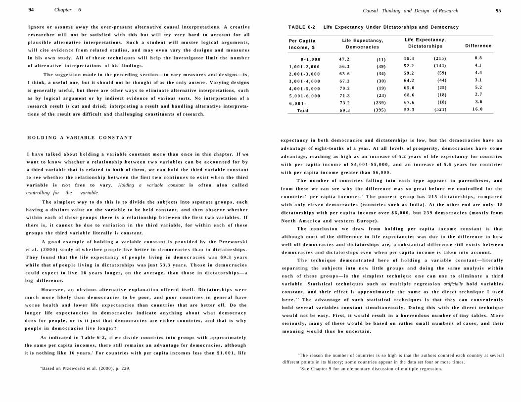
94 Chapter 6

i g n o r e or a s s u m e a w a y the e v e r - p r e s e n t a l ternat ive c a u s a l in terpre ta t ions . A c r e a t i v e

r e s e a r c h e r w i l l no t be s a t i s f i e d w i t h th i s but w i l l try v e r y hard to a c c o u n t for al l

p l a u s i b l e a l t ernat ive in terpre ta t ions . S u c h a s t u d e n t w i l l m u s t e r l o g i c a l a r g u m e n t s ,

w i l l c i t e e v i d e n c e f r o m re la ted s t u d i e s , and m a y e v e n vary the d e s i g n s a n d m e a s u r e s

i n h i s o w n s tudy. A l l o f t h e s e t e c h n i q u e s w i l l h e l p t h e i n v e s t i g a t o r l i m i t t h e n u m b e r

o f a l t ernat ive in terpreta t ions o f h i s f i n d i n g s .

T h e s u g g e s t i o n m a d e i n the preced ing s e c t i o n — t o vary m e a s u r e s and d e s i g n s — i s ,

I think, a useful o n e , but i t s h o u l d not be thought of as the o n l y answer . Varying d e s i g n s

i s genera l ly useful , but there are other w a y s to e l imina te alternative interpretations, such

as by log ica l argument or by indirect e v i d e n c e o f var ious sorts. No interpretation of a

research result is cut and dried; interpreting a result and handl ing alternative interpreta­

t ions of the result are difficult and c h a l l e n g i n g const i tuents of research.

H O L D I N G A V A R I A B L E C O N S T A N T

I h a v e t a l k e d about h o l d i n g a var iab le c o n s t a n t m o r e than o n c e in this chapter . I f we

w a n t t o k n o w w h e t h e r a r e l a t i o n s h i p b e t w e e n t w o v a r i a b l e s c a n b e a c c o u n t e d for b y

a third v a r i a b l e that i s r e la t ed to b o t h o f t h e m , we c a n h o l d the third v a r i a b l e c o n s t a n t

t o s e e w h e t h e r the r e l a t i o n s h i p b e t w e e n the first t w o c o n t i n u e s t o e x i s t w h e n the third

v a r i a b l e is no t free to vary. Holding a variable constant is o f t e n a l s o c a l l e d

controlling for the variable.

T h e s i m p l e s t w a y t o d o this i s t o d i v i d e the s u b j e c t s in to separate g r o u p s , e a c h

h a v i n g a d i s t i n c t v a l u e o n the v a r i a b l e t o b e h e l d c o n s t a n t , a n d t h e n o b s e r v e w h e t h e r

w i t h i n e a c h o f t h e s e g r o u p s there i s a r e l a t i o n s h i p b e t w e e n t h e f i r s t t w o v a r i a b l e s . I f

there i s , i t c a n n o t be d u e to var ia t ion in the third var iab le , for w i t h i n e a c h o f t h e s e

g r o u p s the third v a r i a b l e l i t era l ly i s c o n s t a n t .

A g o o d e x a m p l e o f h o l d i n g a var iab le c o n s t a n t i s p r o v i d e d by the P r z e w o r s k i

e t al . ( 2 0 0 0 ) s t u d y o f w h e t h e r p e o p l e l i v e bet ter i n d e m o c r a c i e s than i n d i c t a t o r s h i p s .

T h e y f o u n d that the l i fe e x p e c t a n c y o f p e o p l e l i v ing i n d e m o c r a c i e s w a s 6 9 . 3 y e a r s

w h i l e that o f p e o p l e l i v i n g i n d i c t a t o r s h i p s w a s j u s t 5 3 . 3 y e a r s . T h o s e i n d e m o c r a c i e s

c o u l d e x p e c t t o l i v e 1 6 y e a r s l o n g e r , o n the a v e r a g e , than t h o s e i n d i c t a t o r s h i p s — a

b i g d i f f e r e n c e .

H o w e v e r , a n o b v i o u s a l t ernat ive e x p l a n a t i o n o f f e r e d itself . D i c t a t o r s h i p s w e r e

m u c h m o r e l i k e l y than d e m o c r a c i e s t o b e poor , a n d p o o r c o u n t r i e s i n g e n e r a l h a v e

w o r s e h e a l t h and l o w e r l i fe e x p e c t a n c i e s than c o u n t r i e s that are bet ter off. D o the

l o n g e r l i fe e x p e c t a n c i e s i n d e m o c r a c i e s i n d i c a t e a n y t h i n g a b o u t w h a t d e m o c r a c y

d o e s for p e o p l e , o r i s i t j u s t that d e m o c r a c i e s are r i c h e r c o u n t r i e s , a n d that i s w h y

p e o p l e i n d e m o c r a c i e s l i v e l o n g e r ?

A s ind ica ted i n Table 6 - 2 , i f w e d i v i d e countr i e s in to g r o u p s w i t h a p p r o x i m a t e l y

the s a m e per capi ta i n c o m e s , there still r emains an advantage for d e m o c r a c i e s , a l t h o u g h

i t i s n o t h i n g l ike 16 y e a r s . 8 F o r countr i e s w i t h per capi ta i n c o m e s l e s s than $ 1 , 0 0 1 , l i fe

"Based on Przeworski et al. (2000), p. 229.

Causal Thinking and Design of Research 95

TABLE 6-2 Life Expectancy Under Dictatorships and Democracy

Per Capita Income, $

Life Expectancy, Democracies

Life Expectancy, Dictatorships Difference

0 - 1 , 0 0 0 4 7 . 2 (11) 4 6 . 4 (215) 0 .8

1 , 0 0 1 - 2 , 0 0 0 5 6 . 3 (39) 5 2 . 2 (144) 4.1

2 , 0 0 1 - 3 , 0 0 0 6 3 . 6 (34) 5 9 . 2 (59) 4 . 4

3 , 0 0 1 - 4 , 0 0 0 6 7 . 3 (30) 6 4 . 2 (44) 3.1

4 , 0 0 1 - 5 , 0 0 0 7 0 . 2 (19) 6 5 . 0 (25) 5.2

5 , 0 0 1 - 6 , 0 0 0 7 1 . 3 (23) 6 8 . 6 (18) 2 . 7

6 , 0 0 1 - 7 3 . 2 (239) 6 7 . 6 (18) 3 .6

Total 6 9 . 3 (395) 5 3 . 3 (521) 1 6 . 0

e x p e c t a n c y in both d e m o c r a c i e s and dictatorships i s low, but the d e m o c r a c i e s h a v e an

a d v a n t a g e o f e ight - tenths o f a year. At all l e v e l s o f prosperity, d e m o c r a c i e s h a v e s o m e

a d v a n t a g e , reach ing as h i g h as an increase o f 5 . 2 years o f l ife e x p e c t a n c y for countr ies

w i t h per capita i n c o m e o f $ 4 , 0 0 1 - $ 5 , 0 0 0 , and a n increase o f 5 . 6 years for countr i e s

w i t h per capita i n c o m e greater than $ 6 , 0 0 0 .

T h e n u m b e r o f c o u n t r i e s f a l l i n g in to e a c h t y p e a p p e a r s i n p a r e n t h e s e s , a n d

f r o m t h e s e w e c a n s e e w h y the d i f f e r e n c e w a s s o great b e f o r e w e c o n t r o l l e d for the

c o u n t r i e s ' per cap i ta i n c o m e s . 9 T h e p o o r e s t g r o u p h a s 2 1 5 d i c t a t o r s h i p s , c o m p a r e d

w i t h o n l y e l e v e n d e m o c r a c i e s ( c o u n t r i e s s u c h a s I n d i a ) . A t the o ther e n d are o n l y 1 8

d i c t a t o r s h i p s w i t h p e r c a p i t a i n c o m e o v e r $ 6 , 0 0 0 , but 2 3 9 d e m o c r a c i e s ( m o s t l y f r o m

N o r t h A m e r i c a and w e s t e r n E u r o p e ) .

T h e c o n c l u s i o n w e d r a w f r o m h o l d i n g p e r cap i ta i n c o m e c o n s t a n t i s that

a l t h o u g h m o s t o f the d i f f erence i n l i fe e x p e c t a n c i e s w a s d u e t o the d i f f erence i n h o w

w e l l o f f d e m o c r a c i e s a n d d ic ta torsh ips are, a substant ia l d i f f erence stil l e x i s t s b e t w e e n

d e m o c r a c i e s and d ic ta torsh ips e v e n w h e n per capi ta i n c o m e i s taken into a c c o u n t .

T h e t e c h n i q u e d e m o n s t r a t e d h e r e o f h o l d i n g a var iab le c o n s t a n t — l i t e r a l l y

s e p a r a t i n g the s u b j e c t s i n t o n e w litt le g r o u p s a n d d o i n g the s a m e a n a l y s i s w i t h i n

e a c h o f t h e s e g r o u p s — i s t h e s i m p l e s t t e c h n i q u e o n e c a n u s e t o e l i m i n a t e a third

var iab l e . S tat i s t i ca l t e c h n i q u e s s u c h as m u l t i p l e r e g r e s s i o n artificially h o l d v a r i a b l e s

c o n s t a n t , a n d the ir e f f e c t i s a p p r o x i m a t e l y the s a m e as the d irec t t e c h n i q u e I u s e d

h e r e . 1 0 T h e a d v a n t a g e o f s u c h stat is t ical t e c h n i q u e s i s that t h e y c a n c o n v e n i e n t l y

h o l d s e v e r a l var iab le s c o n s t a n t s i m u l t a n e o u s l y . D o i n g this w i t h the d irec t t e c h n i q u e

w o u l d no t be e a s y . First , i t w o u l d result in a h o r r e n d o u s n u m b e r o f t iny t a b l e s . M o r e

s e r i o u s l y , m a n y o f t h e s e w o u l d b e b a s e d o n rather s m a l l n u m b e r s o f c a s e s , a n d their

m e a n i n g w o u l d thus b e u n c e r t a i n .

9 The reason the number of countries is so high is that the authors counted each country at several

different points in its history; some countries appear in the data set four or more times. l 0 See Chapter 9 for an elementary discussion of multiple regression.

96 Chapter 6

F U R T H E R D I S C U S S I O N

I have presented here only a few examples of the more commonly used research

designs, and my analysis of them has included only a sample of the possible alternative

explanations for each design. A more complete treatment of research design, excellent

and readable, is provided in Thomas D. Cook and Donald T. Campbel l 's Quasi-

experimentation: Design and Analysis Issues for Field Setting (1979); or more recent

and even more complete (but not quite as readable), Wi l l iam R. Shadish, Thomas D.

Cook , and Donald T. Campbel l Experimental and Quasi-Experimental Designs for

Generalized Causal Inference (2002). I have relied heavily on their approach in this

chapter. Christopher H. A c h e n ' s The Statistical Analysis of Quasi-experiments (1986)

explores these issues with great w isdom; Chapters 1 and 2 are easily accessible to

readers with limited technical preparation. A good treatment of the concept of "cause"

in relation to research design is found in B la lock (1964, Chapters 1 and 2). Tingsten

(1937) provides an example of unusually careful and creative interpretations,

developed in the face of quite l imited research designs. Several interesting examples of

improvised research designs in field research on animal behavior can be found in

Tinbergen (1968).

T h e literature on the use of true experiments in poli t ical sc ience is burgeoning.

G o o d examples are K i n d e r and Palfrey (1993); a special issue of the journa l Political

Analysis (volume 10, no. 4, A u t u m n 2002) ; and a special issue, edited by Dona ld

Green and A l a n Gerber, of American Behavioral Scientist (volume 48, no. 1, January

2004) .

O n e question that you might consider in connect ion with this chapter is : W h y

should theory-oriented, empir ica l polit ical research be based almost exc lus ive ly on

causal relationships rather than on relationships in general?

So far in this book we have looked at how you can develop a research question,

measure the variables involved, and look for relationships among them to provide

answers to the research question. A further important factor underl ies this whole

process, however. To do all these things, you must select a set of observations to look

at, and your selection of cases can sharply affect or even distort what you wi l l find.

Further, it is often the case that the "select ion" occurs by subtle processes other than

your own choice. In this chapter I want to alert you to the importance of case

select ion (whether it is done by you or by nature), and to show you some basic

principles that w i l l help you to select cases in w a y s that w i l l al low you a clean

examination of your research question.

A central theme in this book, w h i c h you saw especial ly in the two chapters on

measurement and w h i c h you wi l l see again in later chapters, is that we need to

construct our research operations so that the relationships we observe among the

variables we have measured mirror faithfully the theoretical relationships we are

interested in. (This was the point of F igure 4-1 , for instance.) It w i l l not surprise you,

then, that case selection is judged by how wel l it produces observed relationships that

faithfully mirror the theoretical relationships we are trying to test.

Consider the fol lowing examples:

• I described earlier the strange case of the Literary Digest, w h i c h in 1936

predicted that F rank l in Roosevel t would lose the election by a landsl ide on the basis

of questionnaires sent to subscribers to their magazine, car owners, and those having

telephone service (not a representative group of A m e r i c a n voters in those days)

(see pp. 5 0 - 5 1 ) . T h e cases they had chosen to look at did not faithfully mirror the

A m e r i c a n electorate.

97

98 Chapter 7

• College students taking psychology tests are routinely used for experiments to measure psychological processes. For instance, an experiment using college students might study the effect of drinking coffee on one's ability to memorize long strings of numbers. Researchers justify doing this by arguing that the processes they are studying are universal, so even though their test subjects are not at all representative of the human population, that does not matter. The relationship they are looking for would be expected to be the same in any kind of group of people, so their students are as good as any other for the test.

• Most graduate departments in political science admit students to their programs based in part on each student's scores on the Graduate Record Examination (GRE). From time to time, a department will consider dropping the exam because when one looks at the performance of graduate students in the department, how they did on the GRE has little to do with how well they have done in the graduate program. Therefore, it is argued, the test is a nearly irrelevant predictor of success in the graduate program and should be dropped as a tool for assessment.

However, this argument relies on data from those admitted to the program to generalize to the population of all students who might apply to the program. Clearly, the students admitted into the program are an atypical sample from the population; they all did well enough on the GRE to get into the program. Would students who did badly on the GRE do well in the program? We cannot know, because no such students are in the group we are able to observe.

In this case, selection of a potentially biased sample did not result from a decision the researcher made, but inheres in the situation. Nature did it.

• John Zaller (1998), studying whether incumbent members of Congress had extra advantages in garnering votes, had to work with another selection problem dealt by nature. His theory predicted that incumbent members' safety from electoral defeat, as measured by their share of the vote, would increase with every term they served, but at a decreasing rate. So he examined the vote margins of incumbents running for reelection, at varying levels of seniority. However, a number of seats were uncontested, because the incumbent was so safe that no one wanted to take her on. So the available set of congressional races consisted only of those districts in which someone felt it made sense to challenge the incumbent.

Zaller stated his problem:

To set [these races] aside, as is sometimes done, would be to set aside those cases in

which incumbents have been most successful in generating electoral security, thereby

understating the amount of electoral security that develops. On the other hand, to regard

victory in an uncontested race as evidence that the MC [member of congress] has

captured 100 percent of the vote would probably exaggerate M C s ' actual level of

support, (p. 136)

In other words, if he ignored the selection problem, he would understate the amount of safety that long-time incumbents accrue. But if instead he treated the unchal­lenged incumbents as having gotten 100 percent of the vote, he would be overstating

Selection of Observations for Study 99

their safety. (His approximated solution was to estimate from other factors the vote that the unchallenged incumbents would have gotten if they had been challenged, and then to insert those simulated estimates as the observations for the unchallenged incumbents—not a perfect solution, but the one that made the best approximation.)

• The general understanding of the new democracies of eastern Europe has been that unless they are culturally homogeneous as Poland is, they are "ethnic powderkegs" that had been held in check only by Soviet repression, and are now prone to explode in ethnic violence. As Mihaela Mihaelescu (2004) has pointed out, however, this general impression has come about because almost all scholars who looked at ethnic conflict in new eastern European democracies were drawn to the dramatic outbreaks of violence in the former Yugoslavia. In fact, of fourteen new states in Eastern Europe with significant ethnic minorities, only four experienced violent ethnic conflict, and three of these were various parts of former Yugoslavia.

In this case, scholars' attraction to the dramatic cases led to a strangely "selected" body of scholarship, in which the full range of possibilities did not get examined.

SAMPLING FROM A POPULATION OF POTENTIAL OBSERVATIONS

Both the Literary Digest example and the discussion of using college students to generalize to all adults are examples of the problem of sampling. We usually cannot study all possible observations to which our theory applies. We cannot, for example, ask every American adult how he or she expects to vote in an election. And, though it would be (barely) possible to do detailed analysis and fieldwork in each country of the world, limitations of time and resources usually bar us from doing so. As a result, we usually work with a sample drawn from the universe of all possible observations to which a theory applies. As noted earlier, the guiding rule in choosing observations for study is that the relationships we are looking for in the full universe of possible cases should be mirrored faithfully among the observations we are using.

Random Sampling

When we are able to draw a fairly large number of observations, the "Cadillac" method is to draw a random sample from the full population of possible cases. In random sampling it is purely a matter of chance which cases from the full population end up in the sample for observation; that is, each member of the population has an equal chance of being drawn for the sample. It is as if we had flipped coins for each possible case and, say, admitted into the sample any case that got heads ten times in a row. (In reality, scholars use computer-generated random numbers to identify which members of the full population should join the sample for observation.)

100 Chapter 7

If a sample has been drawn randomly, we are assured that any relationship in which we are interested should be mirrored faithfully in the sample, at least in the sense that, across repeated samplings of this sort, on the average the relationships we would see would be the same as the relationship in the full population. Even random samples will diverge by accident from the full popula­tion. For instance, although there is a "gender gap" in American voting, with men favoring the Republican party more than women do, it would not be unusual for a sample of ten Americans to include a group of women who were more Republican than the men in the sample. Since in fact men are more likely to be Republicans than women are, most samples of ten Americans would show men to be the more Republican, but it would still happen fairly often, by chance, that the ten people you drew for a sample would show the reverse of that. If you took a large number of such samples, however, and averaged them, the average expres­sion of the gender gap would almost surely mirror faithfully the gender gap in the full population.

The principle here is the same as that in randomized experiments, which we looked at in Chapter 6. In randomized experiments, two groups are randomly chosen, so they cannot be expected to differ in any significant way that could inter­fere with a causal interpretation from the experiment. In other words, randomization ensures that any two groups chosen are essentially alike. But if that is true in experiments, it must also be true when trying to generalize to a population from a sample. If any group chosen randomly from the population can be expected to be essentially the same as any other, then they must all be essentially the same as the full population.

How much variation there is from one random sample to another is hugely influenced by the size of the sample. The larger the sample, the less variation there will be from one time to another when we draw samples and look at a relationship. If you drew samples of a thousand Americans, for instance, it would happen only rarely that you could have come up with a group among whom the women were more Republican than the men. (Review the discussion of the Law of Large Numbers, p. 61. We saw there that variation in anything we are observing becomes less variable as we use larger and larger samples to examine it.)

One nice thing about random samples is that there is a very precisely worked out mathematical system to ascertain, for a sample of any given size, exactly how likely it is that the sample result is any given distance from what you would have seen in the population. It is this mathematical system that allows pollsters to say of a national poll, for example, that it shows support of 48 percent for George Bush, within an error of plus or minus 3 percentage points.

It always seems surprising that samples do not really need to be all that large to give an accurate rendition of a population. Typically, surveys of American citizens are considered to have sufficient cases for accurately mirroring the population of 302,000,000 if they have questioned a sample of two or three thousand people. It is kind of amazing that just a few thousand out of hundreds of millions would be sufficient to estimate the population to within a couple of percentage points.

Selection of Observations for Study 101

Now, while the true random sample is the Cadillac of sampling, it is rarely used, at least for large populations. For relatively small populations, such as the population of a city, true random sampling is often feasible, and is then, of course, the method of choice. But you can imagine what it would cost to sample the U.S. population in a truly random way—sending an interviewer to interview a single person in Menominee, Wisconsin, another to interview a person in San Diego, and so on.

Quasi-random Sampling

When a large population is involved, various methods exist to draw "quasi-random" approximations to a random sample. The National Election Study at the University of Michigan uses what is called a "cluster sample": About 100 localities are first selected, and then, within each of these, a certain number of individuals are randomly chosen for the sample. This allows the survey to use approximately 100 interviewers, one based in each of the localities chosen. Then, instead of having interviewers fly or drive hundreds of miles for a single interview, each interviewer can readily reach the 20 or 30 subjects randomly selected from her cluster. The end result approximates a random sample closely. And statistical adjustments can be made to take into account the clustered structure of the sample, so that it operates almost exactly like a random sample.

An alternative system is to draw a truly random sample of telephones by having a computer dial telephones randomly ("random digit dialing," or RDD sampling). This allows access to a random sample without the difficulty or expense of getting an interviewer to the person's door, but it is increasingly difficult to draw a sample in this way that represents the broad population accurately. In 1932, at the time of the Literary Digest poll described earlier, the problem with telephone lists was that only the middle class had telephones. Today almost everyone has a telephone, so in principle RDD sampling could work well. But in practice, people's use of their phones varies enough so that the group that can actually be reached by phone at a given time is problematic as a sample. Some people are at work all day, so their telephones will ring at any daytime hour but not be answered unless by a machine. Others are always gone in the evenings. Some telephones have devices to block unsolicited calls. Some families have two phone lines, and therefore would be twice as likely to end up in the sample. RDD samples are rather problematic as approximations of a random sample of the population.

Looking back now at the first two examples stated, we can see from our consideration of random sampling how they might (or might not) be questionable as samples. The Literary Digest poll was drawn before sampling was well understood. Its sample of telephone owners, subscribers to the magazine, and those appearing on state lists of registered automobiles was simply a terrible sample, very much skewed toward the middle class, and would have produced an erroneous prediction any time the middle class voted differently than the population as a whole. The sample of college students, on the other hand, might provide a reasonable basis for drawing psychological conclusions about people in general, even though they are clearly not

102 Chapter 7

a random sample of the full population if we are confident that their psychological processes are the same as psychological processes among the full population. In this case, even though the sample is not random, it is much cheaper than trying to draw a random sample of all people, and can serve as a satisfactory quasi-random sample if processes are indeed the same as for the full population.

Purposive Sampling

Sometimes we deliberately want to sample in a nonrandom way, not just for reasons of efficiency or cost, but because a deliberately constructed, nonrandom sample serves a purpose for our research. If we wanted to compare the political choices of African Americans and whites, for instance, a purely random sample (or good approximation, such as a national cluster sample) would probably not yield enough African American citizens for a good comparison. If it faithfully mirrored the population, it should have about one-eighth of the sample African American, too small a group for reliable comparisons in a sample of the usual size. One solution would be to draw a monstrously large sample, but that would, of course, be very expensive. Another solution, if the purpose of the study is to look at the politics of race, is to draw what is called a "purposive" sample.

A purposive sample does not attempt to replicate the full population. Rather, it draws subjects to maximize variation in the independent variable of interest, so that the relationships we are looking for will be very clear.1 In the preceding example, we could sample African Americans randomly and sample whites randomly, combining them to construct a sample that is half white and half African American. Like all purposive samples, this would not work as a general reflection of the full population. If African Americans were more likely to vote Democratic than whites, for instance, the sample would give an unreasonably high estimate of the Democratic vote. But the one thing for which the sample is going to be used, estimating a relationship or set of relationships based on race, is fine. Since both African Americans and whites have been randomly (or quasi-randomly) selected, an estimate of, say, the news-watching habits of the two races should reflect accurately the difference in news-watching habits in the full population.

One reason that most sampling is random or quasi-random, rather than purposive, is that usually when we draw a sample, it is intended to serve multiple purposes. And we should probably also anticipate that as we proceed with analysis, we might want to look at things in the data other than what we had anticipated when we were first drawing up the sample. A purposive sample works only for the particular independent variable or variables on which we have based the sample. So it is usually safer and more useful to draw up a more general sample, random or quasi-random, rather than one focused just on the single task we start with.

'We will see (pp. 106-108) why we do not draw the sample to maximize variation in the dependent variable.

Selection of Observations for Study 103

Selection of Cases for Case Studies

Another kind of purposive sampling comes into play when we are dealing with such small numbers of cases that random sampling would not be very helpful in any case. A case study is an intensive study of one or a few cases. It might be a study of a particular president's administrative style, an intensive study of the attitudes and ideologies of a few people, or, as it is most frequently seen, a study of some aspect of politics in one or a few countries. In principle, even if we are looking at only two or three cases, random selection of the case or cases would reflect the full population in the long run. But in practice, the Law of Large Numbers is working so weakly when we study only a few cases that the divergence of any case from the full population, though it will be "only random," will still be huge.2 Under these circumstances there is much more to be gained by intelligently choosing the case(s) to pick up the relationship of interest, rather than by randomly drawing the case(s). If we want to study the effect of authoritarian government on economic growth, for instance, it makes sense to seek a couple of authoritarian states and a couple of nonauthoritarian ones for comparison, rather than just taking four randomly chosen states.

CENSORED DATA

The last three of the five examples in the introduction to this chapter were examples of "censored data," instances in which part of tue range of cases to which a theory applies are cut off and unavailable to the researcher, either by the researcher's choice or by circumstances. In the case of GRE scores, any generalization about the importance of test scores is obviously meant to apply to all students who could apply for admission, but the researcher can see the performance only of students who were admitted to the program. John Zaller's theory of congressional elections was obviously meant to apply to all members of Congress, but he could observe election outcomes only for those members who were challenged by an opponent. In the case of ethnic violence in eastern Europe, the theory that ancient hatreds would flare up after Soviet repression was lifted from the region obviously was meant to apply to all eastern European democracies with large ethnic minorities, but scholars had chosen to look only at the dramatic cases in which conflict had actually occured.

The problem of censored data is always severe, because it requires researchers and their readers to make strong assumptions about what "might have been" in the range of data that are not available. Sometimes there are reasonable ways to fill in the spaces. Zaller, for instance, estimated on the basis of other variables what vote unchallenged members could have been expected to receive

2This is a situation that seems to fit Keynes' well-known comment that in the long run we shall all be dead. In principle and in the long run, a randomly selected sample of even just a couple of cases will mirror the full population. But any given couple of cases—for instance, the ones you plan to study—are likely to diverge sharply from the full population.

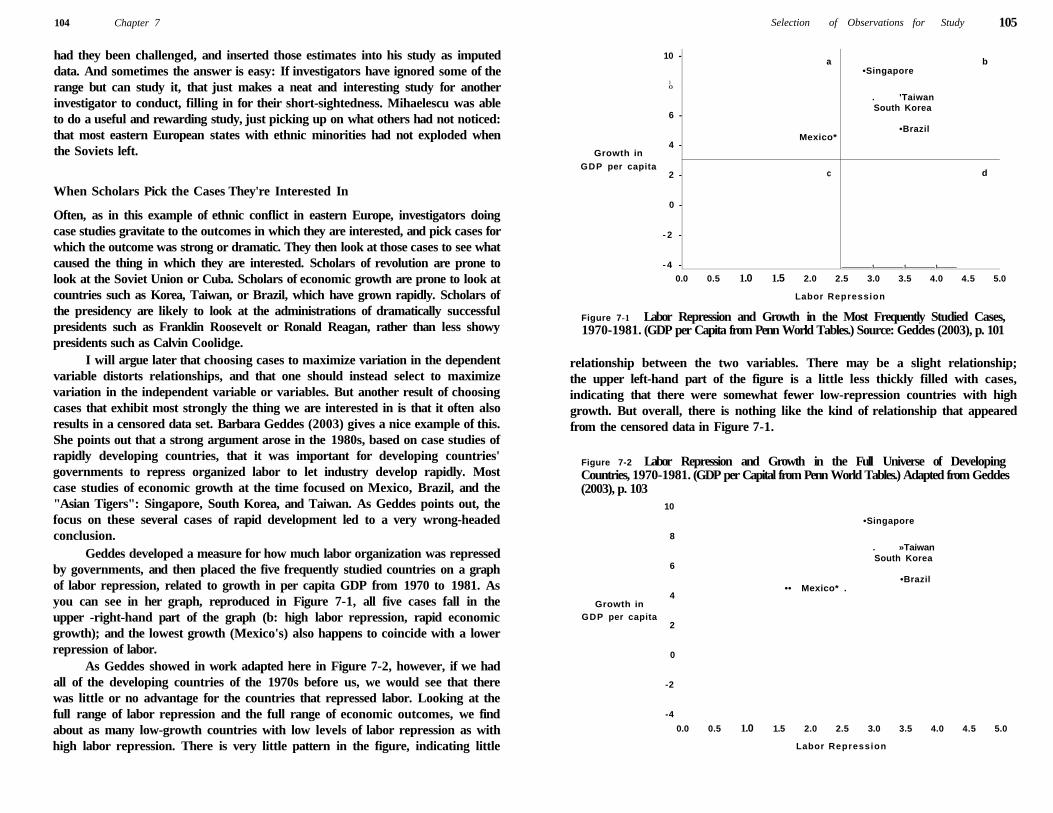
104 Chapter 7

had they been challenged, and inserted those estimates into his study as imputed data. And sometimes the answer is easy: If investigators have ignored some of the range but can study it, that just makes a neat and interesting study for another investigator to conduct, filling in for their short-sightedness. Mihaelescu was able to do a useful and rewarding study, just picking up on what others had not noticed: that most eastern European states with ethnic minorities had not exploded when the Soviets left.

When Scholars Pick the Cases They're Interested In

Often, as in this example of ethnic conflict in eastern Europe, investigators doing case studies gravitate to the outcomes in which they are interested, and pick cases for which the outcome was strong or dramatic. They then look at those cases to see what caused the thing in which they are interested. Scholars of revolution are prone to look at the Soviet Union or Cuba. Scholars of economic growth are prone to look at countries such as Korea, Taiwan, or Brazil, which have grown rapidly. Scholars of the presidency are likely to look at the administrations of dramatically successful presidents such as Franklin Roosevelt or Ronald Reagan, rather than less showy presidents such as Calvin Coolidge.

I will argue later that choosing cases to maximize variation in the dependent variable distorts relationships, and that one should instead select to maximize variation in the independent variable or variables. But another result of choosing cases that exhibit most strongly the thing we are interested in is that it often also results in a censored data set. Barbara Geddes (2003) gives a nice example of this. She points out that a strong argument arose in the 1980s, based on case studies of rapidly developing countries, that it was important for developing countries' governments to repress organized labor to let industry develop rapidly. Most case studies of economic growth at the time focused on Mexico, Brazil, and the "Asian Tigers": Singapore, South Korea, and Taiwan. As Geddes points out, the focus on these several cases of rapid development led to a very wrong-headed conclusion.

Geddes developed a measure for how much labor organization was repressed by governments, and then placed the five frequently studied countries on a graph of labor repression, related to growth in per capita GDP from 1970 to 1981. As you can see in her graph, reproduced in Figure 7-1, all five cases fall in the upper -right-hand part of the graph (b: high labor repression, rapid economic growth); and the lowest growth (Mexico's) also happens to coincide with a lower repression of labor.

As Geddes showed in work adapted here in Figure 7-2, however, if we had all of the developing countries of the 1970s before us, we would see that there was little or no advantage for the countries that repressed labor. Looking at the full range of labor repression and the full range of economic outcomes, we find about as many low-growth countries with low levels of labor repression as with high labor repression. There is very little pattern in the figure, indicating little

Selection of Observations for Study 105

10 -

Q

a •Singapore

b

O -

6 -

. 'Taiwan South Korea

Growth in 4 -

Mexico* •Brazil

GDP per capita 2 -

0 -

- 2 -

- 4 -

c

1 1 1

d

0.0 0.5 1.0 1.5 2.0 2.5 3.0 3.5 4.0 4.5 5.0

Labor Repression

Figure 7-1 Labor Repression and Growth in the Most Frequently Studied Cases, 1970-1981. (GDP per Capita from Penn World Tables.) Source: Geddes (2003), p. 101

relationship between the two variables. There may be a slight relationship; the upper left-hand part of the figure is a little less thickly filled with cases, indicating that there were somewhat fewer low-repression countries with high growth. But overall, there is nothing like the kind of relationship that appeared from the censored data in Figure 7-1.

Figure 7-2 Labor Repression and Growth in the Full Universe of Developing Countries, 1970-1981. (GDP per Capital from Penn World Tables.) Adapted from Geddes (2003), p. 103

Growth in GDP per capita

10

8

6

4

2

0

-2

-4

•• Mexico* .

•Singapore

. »Taiwan South Korea

•Brazil

0.0 0.5 1.0 1.5 2.0 2.5 3.0 3.5 4.0 4.5 5.0

Labor Repression

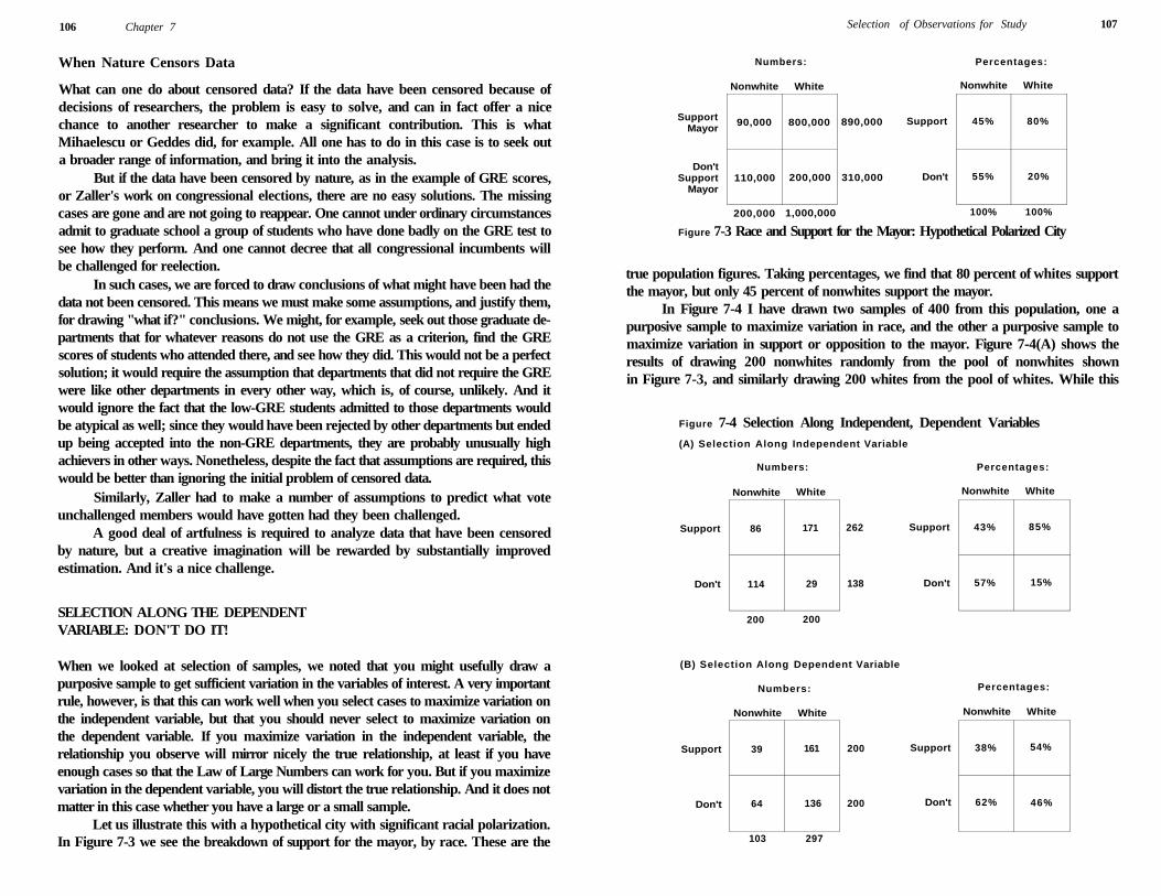
106 Chapter 7

When Nature Censors Data

What can one do about censored data? If the data have been censored because of decisions of researchers, the problem is easy to solve, and can in fact offer a nice chance to another researcher to make a significant contribution. This is what Mihaelescu or Geddes did, for example. All one has to do in this case is to seek out a broader range of information, and bring it into the analysis.

But if the data have been censored by nature, as in the example of GRE scores, or Zaller's work on congressional elections, there are no easy solutions. The missing cases are gone and are not going to reappear. One cannot under ordinary circumstances admit to graduate school a group of students who have done badly on the GRE test to see how they perform. And one cannot decree that all congressional incumbents will be challenged for reelection.

In such cases, we are forced to draw conclusions of what might have been had the data not been censored. This means we must make some assumptions, and justify them, for drawing "what if?" conclusions. We might, for example, seek out those graduate de­partments that for whatever reasons do not use the GRE as a criterion, find the GRE scores of students who attended there, and see how they did. This would not be a perfect solution; it would require the assumption that departments that did not require the GRE were like other departments in every other way, which is, of course, unlikely. And it would ignore the fact that the low-GRE students admitted to those departments would be atypical as well; since they would have been rejected by other departments but ended up being accepted into the non-GRE departments, they are probably unusually high achievers in other ways. Nonetheless, despite the fact that assumptions are required, this would be better than ignoring the initial problem of censored data.

Similarly, Zaller had to make a number of assumptions to predict what vote unchallenged members would have gotten had they been challenged.

A good deal of artfulness is required to analyze data that have been censored by nature, but a creative imagination will be rewarded by substantially improved estimation. And it's a nice challenge.

SELECTION ALONG THE DEPENDENT VARIABLE: DON'T DO IT!

When we looked at selection of samples, we noted that you might usefully draw a purposive sample to get sufficient variation in the variables of interest. A very important rule, however, is that this can work well when you select cases to maximize variation on the independent variable, but that you should never select to maximize variation on the dependent variable. If you maximize variation in the independent variable, the relationship you observe will mirror nicely the true relationship, at least if you have enough cases so that the Law of Large Numbers can work for you. But if you maximize variation in the dependent variable, you will distort the true relationship. And it does not matter in this case whether you have a large or a small sample.

Let us illustrate this with a hypothetical city with significant racial polarization. In Figure 7-3 we see the breakdown of support for the mayor, by race. These are the

Selection of Observations for Study 107

Numbers: Percentages:

Nonwhite White Nonwhite White

Support Mayor

90,000 800,000 890,000 Support 45% 80%

Don't Support

Mayor 110,000 200,000 310,000 Don't 55% 20%

200,000 1,000,000 100% 100%

Figure 7-3 Race and Support for the Mayor: Hypothetical Polarized City

true population figures. Taking percentages, we find that 80 percent of whites support the mayor, but only 45 percent of nonwhites support the mayor.

In Figure 7-4 I have drawn two samples of 400 from this population, one a purposive sample to maximize variation in race, and the other a purposive sample to maximize variation in support or opposition to the mayor. Figure 7-4(A) shows the results of drawing 200 nonwhites randomly from the pool of nonwhites shown in Figure 7-3, and similarly drawing 200 whites from the pool of whites. While this

Figure 7-4 Selection Along Independent, Dependent Variables (A) Selection Along Independent Variable

Numbers: Percentages:

Nonwhite White Nonwhite White

Support 86 171 262 Support 43% 85%

Don't 114 29 138 Don't 57% 15%

200 200

(B) Selection Along Dependent Variable

Numbers:

Nonwhite White

Percentages:

Nonwhite White

Support 39 161 200 Support 38% 54%

Don't 64 136 200 Don't 62% 46%

103 297

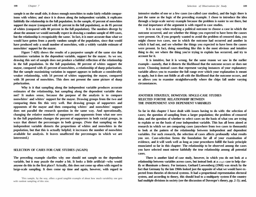
108 Chapter 7

sample is on the small side, it draws enough nonwhites to make fairly reliable compar­isons with whites; and since it is drawn along the independent variable, it replicates faithfully the relationship in the full population. In the sample, 43 percent of nonwhites support the mayor (compared with 45 percent in the full population), as do 85 percent of whites (compared with 80 percent in the full population). The numbers diverge by about the amount we would normally expect in drawing a random sample of 400 cases, but the relationship is recognizably the same.3 In fact, it is more accurate than what we would have gotten from a purely random sample of the population, since that would have produced only a small number of nonwhites, with a widely variable estimate of nonwhites' support for the mayor.

Figure 7-4(B) shows the results of a purposive sample of the same size that maximizes variation in the dependent variable, support for the mayor. As we see, drawing this sort of sample does not produce a faithful reflection of the relationship in the full population. In the full population, 80 percent of whites support the mayor, compared with 45 percent of nonwhites, a relationship of sharp polarization. But the sample maximizing variation in support appears to indicate a considerably weaker relationship, with 54 percent of whites supporting the mayor, compared with 38 percent of nonwhites. This does not present the same picture of sharp polarization.

Why is it that sampling along the independent variable produces accurate estimates of the relationship, but sampling along the dependent variable does not? It makes sense, because the purpose of the analysis is to compare nonwhites' and whites' support for the mayor. Drawing groups from the two and comparing them fits this very well. But drawing groups of supporters and opponents of the mayor and then comparing whites' and nonwhites' support does not parallel the research question in the same way. And operationally, changing the relative numbers of supporters and opponents from what one sees in the full population changes the percent of supporters in both racial groups, in ways that distort the percentages in both groups. (Note that sampling on the independent variable distorts the proportions of whites and nonwhites in the population, but that this is actually helpful; it increases the number of nonwhites available for analysis. It leaves unaffected the percentages in which we are interested.)

SELECTION OF CASES FOR CASE STUDIES (AGAIN)

The preceding example clarifies why one should not sample on the dependent variable, but it may puzzle the reader a bit. It looks a little artificial—why would anyone do this in the first place? Actually, this does not come up often with regard to large-scale sampling. It does come up time and again, however, with regard to

3 This sample, by the way, offers a good tangible example of about how much variability one gets with random sampling of this size.

Selection of Observations for Study 109

intensive studies of one or a few cases (so-called case studies), and the logic there is just the same as the logic of the preceding example. I chose to introduce the idea through a large-scale survey example because the problem is easier to see there, but the real importance of the argument is with regard to case studies.

It is so easy when studying a political outcome to choose a case in which the outcome occurred, and see whether the things you expected to have been the causes were present. Or, if you properly wanted to avoid the problem of censored data, you might choose two cases, one in which the outcome had occurred and another in which it had not, and see whether the things you expected to have been the causes were present. In fact, doing something like this is the most obvious and intuitive thing to do; see where the thing you're trying to explain has occurred, and try to account for it.

It is intuitive, but it is wrong, for the same reason we saw in the earlier example—namely, that it distorts the likelihood that the outcome occurs or does not occur. Choosing instead cases that represent varying instances of your explanatory variable allows you to examine the full range over which your explanation is meant to apply, but it does not fiddle at all with the likelihood that the outcome occurs, and so allows you to examine straightforwardly where the chips fall under varying circumstances.

ANOTHER STRATEGY, HOWEVER: SINGLE-CASE STUDIES SELECTED FORTHE RELATIONSHIP BETWEEN THE INDEPENDENT AND DEPENDENT VARIABLES

So far in this chapter I have dealt with issues having to do with: the selection of cases; the question of sampling from a larger population; the problem of censored data; and the question of whether to select cases on the basis of what you are trying to explain or on the basis of your independent variable. This has all been aimed at research in which we are comparing cases (anywhere from two cases to thousands) to look at the pattern of the relationship between independent and dependent variables. For such research, the selection of cases affects profoundly what results you see. Case-selection forms the foundation for all of your examination of evidence, and it will work well as long as your procedures fulfill the basic principle enunciated so far in this chapter: The relationship to be observed among the cases you have selected must mirror faithfully the true relationship among all potential cases.

There is another kind of case study, however, in which you do not look at a relationship between variables across cases, but instead look at a single case to help clar­ify or illuminate a theory. For instance, Gerhard Loewenberg (1968) was struck by the fact that Germany by the late 1960s looked just the opposite of what we would have ex­pected from theories of electoral systems. It had a proportional representation electoral system, and according to theory, this should lead to a multiparty system if the country had multiple divisions in society (see the discussion of Duverger's theory, pp. 2-3); and,

110 Chapter 7

Germany had demonstrated in the 1920s and 1930s that it did indeed have a richly

divided society. (At its highest, the number of parties represented in the prewar German

Reichstag had been 32!) But by the late 1960s Germany had almost a two-party

system. 4 H o w could this be? Loewenberg studied the German case in depth to see what

had produced this exception to the theory, in order to refine the theory and illuminate

how it worked.

Note that Loewenberg did not p ick this case just in terms of the dependent

variable. He did not s imply p ick a case with a dramatic or interesting outcome.

Rather, he p icked it because of the combination of the electoral system and historic

divisions in society (independent variables) and the party system (dependent

variable). W h e n a case study is being used in this w a y — n o t to test a theory by trying

it out to see how wel l it works , but rather to develop the theory by looking in detail at

a case in w h i c h the theory is work ing in particular w a y s — we should not ignore the

dependent variable in selecting our case. B u t we should also not select the case just

in terms of the dependent variable. Rather, we should p ick the case because of how

the theory appears to be work ing, as indicated by the combination of dependent and

independent variables. A n d , we should then be clear that we are not providing a test

of the theory. Rather, this is a strategy for further refinement of the theory. 5

F U R T H E R D I S C U S S I O N

John Gerr ing (2007) provides a comprehensive and intelligent review of case selection.

Geddes (2003) has a very nice chapter, "How the C a s e s You Choose Affect the

A n s w e r s Y o u Get." A good, though fairly technical, treatment of censored data is

presented in Przeworski et al . (2000) in an appendix, "Select ion Models." Another

good treatment of case selection is K i n g , Keohane, and Verba (1994), Chapter 4.

4 Since then the system has moved back somewhat toward multipartism. Three parties were represented in the parliament in the 1960s, with the two largest (the Social Democrats and the Christian democrats) holding about 90 percent of the seats. Currently there are five parties represented, and the "big two" have 73 percent of the seats.

5 This argument is developed in Shively (2006).

Chapter 8

©

Measuring Relationships for Interval Data

In Chapter 6 we were concerned generally wi th "relat ionships" between independent

and dependent variables. That is , we wanted to see whether the presence or absence

of a test factor affected the value of the dependent variable. T h i s was too simple, for

two reasons.

F i rst , as noted in footnote 5 in that chapter, the test factor in field research is

frequently not something that is s imply present or absent; rather, it takes on a variety

of values. Our task then is not just to see whether the presence or absence of a test

factor affects the value of the dependent variable, but instead, to see whether and how

the value of the independent variable affects the value of the dependent variable. For

example, in relating education to income, we do not treat people simply as "educated"

or "not educated." They have varying amounts of education, and our task is to see

whether the amount of education a person has affects his or her income.

Second , "relat ionship" cannot be d ichotomized, although I treated it as a

dichotomy in Chapter 6, to ease the presentation there. T w o variables are not s imply

related or not related. Relat ionships vary in two ways : first, in how strongly the

independent variable affects the dependent variable. F o r instance, education might

have only a minor effect on income. T h e average income of col lege graduates might

be $33,000 and the average income of high school dropouts might be $30,000. Or,

it might have a major effect. Co l lege graduates might average $50 ,000 , whi le high

school dropouts average $15,000.

Relat ionships also vary in how completely the independent variable deter­

mines scores on the dependent variable. Co l lege graduates might average $50,000

income and high school dropouts $15,000, for instance, yet there might stil l be much

variation in incomes that cou ld not be attributed to variation in people 's education.

S o m e college graduates might make only $10,000 a year and some high school

dropouts might make $80,000 or $90,000 a year, even though the average income of

111

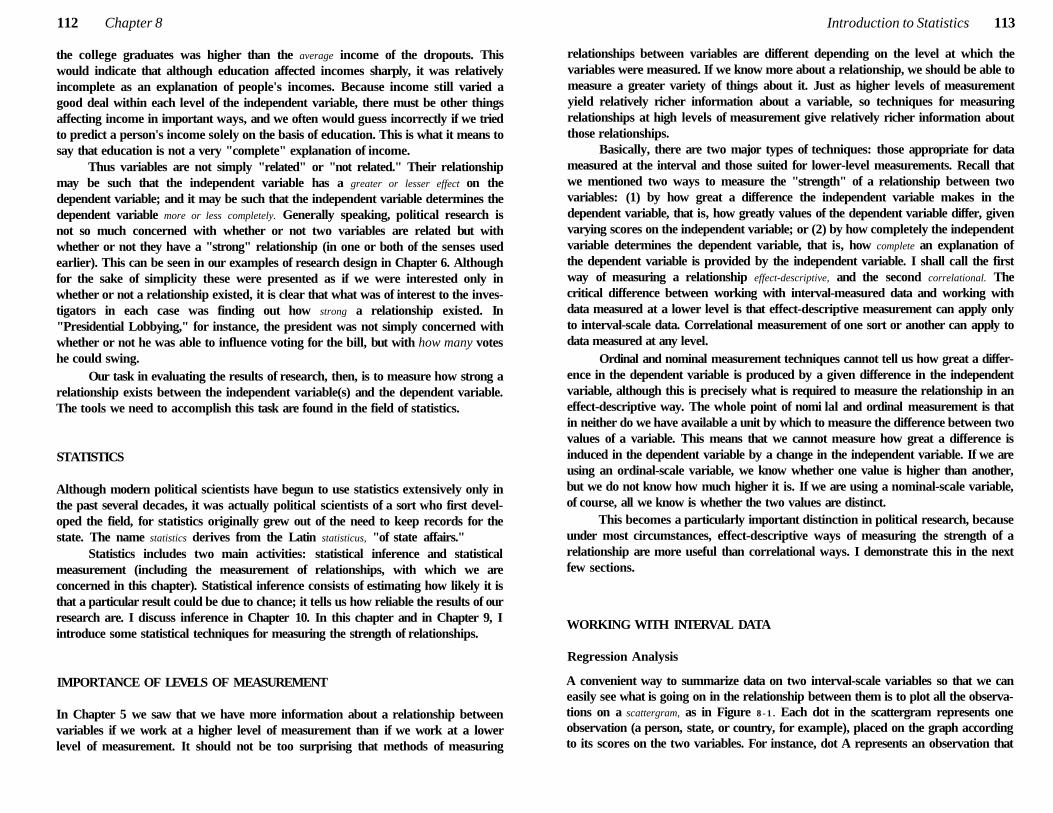
112 Chapter 8

the college graduates was higher than the average income of the dropouts. This would indicate that although education affected incomes sharply, it was relatively incomplete as an explanation of people's incomes. Because income still varied a good deal within each level of the independent variable, there must be other things affecting income in important ways, and we often would guess incorrectly if we tried to predict a person's income solely on the basis of education. This is what it means to say that education is not a very "complete" explanation of income.

Thus variables are not simply "related" or "not related." Their relationship may be such that the independent variable has a greater or lesser effect on the dependent variable; and it may be such that the independent variable determines the dependent variable more or less completely. Generally speaking, political research is not so much concerned with whether or not two variables are related but with whether or not they have a "strong" relationship (in one or both of the senses used earlier). This can be seen in our examples of research design in Chapter 6. Although for the sake of simplicity these were presented as if we were interested only in whether or not a relationship existed, it is clear that what was of interest to the inves­tigators in each case was finding out how strong a relationship existed. In "Presidential Lobbying," for instance, the president was not simply concerned with whether or not he was able to influence voting for the bill, but with how many votes he could swing.

Our task in evaluating the results of research, then, is to measure how strong a relationship exists between the independent variable(s) and the dependent variable. The tools we need to accomplish this task are found in the field of statistics.

STATISTICS

Although modern political scientists have begun to use statistics extensively only in the past several decades, it was actually political scientists of a sort who first devel­oped the field, for statistics originally grew out of the need to keep records for the state. The name statistics derives from the Latin statisticus, "of state affairs."

Statistics includes two main activities: statistical inference and statistical measurement (including the measurement of relationships, with which we are concerned in this chapter). Statistical inference consists of estimating how likely it is that a particular result could be due to chance; it tells us how reliable the results of our research are. I discuss inference in Chapter 10. In this chapter and in Chapter 9, I introduce some statistical techniques for measuring the strength of relationships.

IMPORTANCE OF LEVELS OF MEASUREMENT

In Chapter 5 we saw that we have more information about a relationship between variables if we work at a higher level of measurement than if we work at a lower level of measurement. It should not be too surprising that methods of measuring

Introduction to Statistics 113

relationships between variables are different depending on the level at which the variables were measured. If we know more about a relationship, we should be able to measure a greater variety of things about it. Just as higher levels of measurement yield relatively richer information about a variable, so techniques for measuring relationships at high levels of measurement give relatively richer information about those relationships.

Basically, there are two major types of techniques: those appropriate for data measured at the interval and those suited for lower-level measurements. Recall that we mentioned two ways to measure the "strength" of a relationship between two variables: (1) by how great a difference the independent variable makes in the dependent variable, that is, how greatly values of the dependent variable differ, given varying scores on the independent variable; or (2) by how completely the independent variable determines the dependent variable, that is, how complete an explanation of the dependent variable is provided by the independent variable. I shall call the first way of measuring a relationship effect-descriptive, and the second correlational. The critical difference between working with interval-measured data and working with data measured at a lower level is that effect-descriptive measurement can apply only to interval-scale data. Correlational measurement of one sort or another can apply to data measured at any level.

Ordinal and nominal measurement techniques cannot tell us how great a differ­ence in the dependent variable is produced by a given difference in the independent variable, although this is precisely what is required to measure the relationship in an effect-descriptive way. The whole point of nomi lal and ordinal measurement is that in neither do we have available a unit by which to measure the difference between two values of a variable. This means that we cannot measure how great a difference is induced in the dependent variable by a change in the independent variable. If we are using an ordinal-scale variable, we know whether one value is higher than another, but we do not know how much higher it is. If we are using a nominal-scale variable, of course, all we know is whether the two values are distinct.

This becomes a particularly important distinction in political research, because under most circumstances, effect-descriptive ways of measuring the strength of a relationship are more useful than correlational ways. I demonstrate this in the next few sections.

WORKING WITH INTERVAL DATA

Regression Analysis

A convenient way to summarize data on two interval-scale variables so that we can easily see what is going on in the relationship between them is to plot all the observa­tions on a scattergram, as in Figure 8 - 1 . Each dot in the scattergram represents one observation (a person, state, or country, for example), placed on the graph according to its scores on the two variables. For instance, dot A represents an observation that

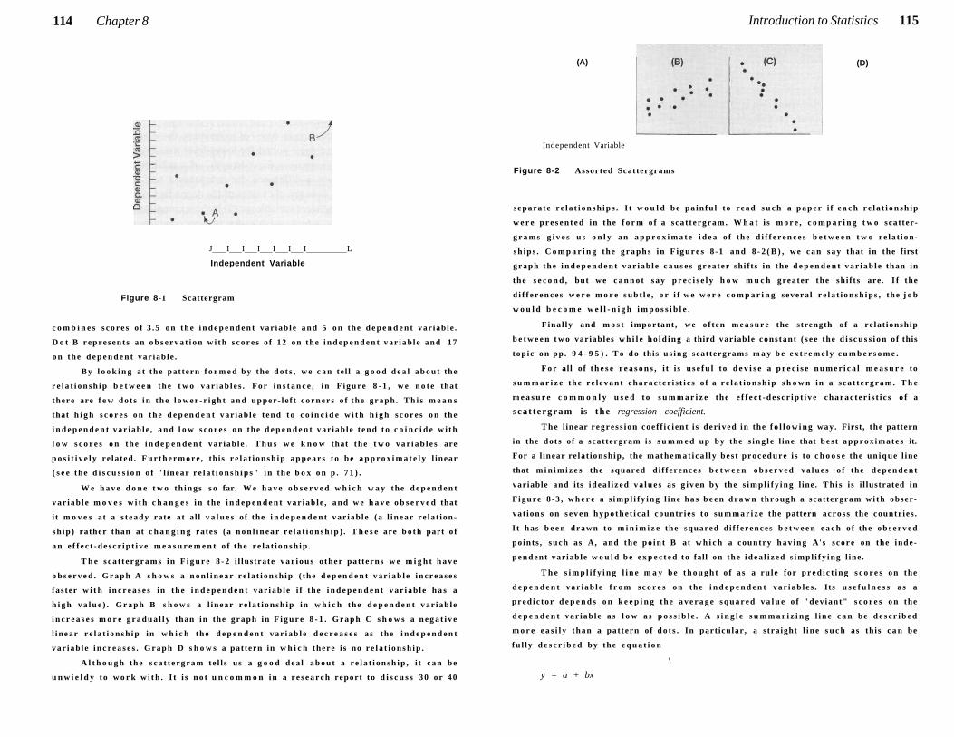
114 Chapter 8

J I I I I I I L

Independent Variable

Figure 8-1 Scattergram

c o m b i n e s s c o r e s o f 3 .5 o n the i n d e p e n d e n t var iab le a n d 5 o n the d e p e n d e n t var iable .

D o t B r e p r e s e n t s an o b s e r v a t i o n w i t h s c o r e s o f 12 on the i n d e p e n d e n t var iab le a n d 17

o n the d e p e n d e n t var iab le .

B y l o o k i n g a t the pat tern f o r m e d b y the d o t s , w e c a n te l l a g o o d d e a l a b o u t the

r e l a t i o n s h i p b e t w e e n the t w o v a r i a b l e s . F o r i n s t a n c e , i n F i g u r e 8 - 1 , w e n o t e that

there are f e w d o t s i n t h e l o w e r - r i g h t a n d upper - l e f t c o r n e r s o f the graph . T h i s m e a n s

that h i g h s c o r e s o n the d e p e n d e n t var iab le t end t o c o i n c i d e w i t h h i g h s c o r e s o n the

i n d e p e n d e n t var iab le , a n d l o w s c o r e s o n the d e p e n d e n t var iab le t e n d t o c o i n c i d e w i t h

l o w s c o r e s o n the i n d e p e n d e n t var iab le . T h u s w e k n o w that the t w o v a r i a b l e s are

p o s i t i v e l y re la ted . F u r t h e r m o r e , th is r e l a t i o n s h i p a p p e a r s t o b e a p p r o x i m a t e l y l inear

( s e e the d i s c u s s i o n o f " l inear r e l a t i o n s h i p s " i n t h e b o x o n p . 7 1 ) .

W e h a v e d o n e t w o t h i n g s s o far. W e h a v e o b s e r v e d w h i c h w a y the d e p e n d e n t

v a r i a b l e m o v e s w i t h c h a n g e s i n the i n d e p e n d e n t var iab le , a n d w e h a v e o b s e r v e d that

i t m o v e s at a s t e a d y rate at a l l v a l u e s of the i n d e p e n d e n t var iab le (a l i n e a r re la t ion­

s h i p ) rather than a t c h a n g i n g rates (a n o n l i n e a r r e l a t i o n s h i p ) . T h e s e are b o t h part o f

a n e f f e c t - d e s c r i p t i v e m e a s u r e m e n t o f the r e l a t i o n s h i p .

T h e s c a t t e r g r a m s i n F i g u r e 8 - 2 i l lustrate v a r i o u s o ther pat terns w e m i g h t h a v e

o b s e r v e d . G r a p h A s h o w s a n o n l i n e a r r e l a t i o n s h i p ( the d e p e n d e n t v a r i a b l e i n c r e a s e s

fas ter w i t h i n c r e a s e s in the i n d e p e n d e n t v a r i a b l e i f the i n d e p e n d e n t v a r i a b l e h a s a

h i g h v a l u e ) . G r a p h B s h o w s a l inear r e l a t i o n s h i p in w h i c h the d e p e n d e n t var iab le

i n c r e a s e s m o r e g r a d u a l l y than in the g r a p h in F i g u r e 8 - 1 . G r a p h C s h o w s a n e g a t i v e

l inear r e l a t i o n s h i p i n w h i c h the d e p e n d e n t v a r i a b l e d e c r e a s e s a s the i n d e p e n d e n t

v a r i a b l e i n c r e a s e s . G r a p h D s h o w s a pattern in w h i c h there i s no r e l a t i o n s h i p .

A l t h o u g h the s c a t t e r g r a m te l l s us a g o o d dea l a b o u t a r e l a t i o n s h i p , i t c a n be

u n w i e l d y t o w o r k w i t h . I t i s n o t u n c o m m o n i n a r e s e a r c h report t o d i s c u s s 3 0 o r 4 0

Introduction to Statistics 115

(A) (D)

Independent Variable

Figure 8-2 Assorted Scattergrams

separate r e l a t i o n s h i p s . I t w o u l d be p a i n f u l to read s u c h a p a p e r i f e a c h r e l a t i o n s h i p

w e r e p r e s e n t e d i n the f o r m o f a s ca t t ergram. W h a t i s m o r e , c o m p a r i n g t w o scatter­

g r a m s g i v e s u s o n l y a n a p p r o x i m a t e i d e a o f the d i f f e r e n c e s b e t w e e n t w o r e l a t i o n ­

s h i p s . C o m p a r i n g the g r a p h s i n F i g u r e s 8 -1 and 8 - 2 ( B ) , w e c a n s a y that i n the first

g r a p h the i n d e p e n d e n t v a r i a b l e c a u s e s grea ter sh i f t s i n the d e p e n d e n t v a r i a b l e than i n

the s e c o n d , but w e c a n n o t s a y p r e c i s e l y h o w m u c h greater the sh i f t s are. I f the

d i f f e r e n c e s w e r e m o r e s u b t l e , o r i f w e w e r e c o m p a r i n g severa l r e l a t i o n s h i p s , the j o b

w o u l d b e c o m e w e l l - n i g h i m p o s s i b l e .

F ina l ly and m o s t important , we o f ten m e a s u r e the strength o f a re lat ionship

b e t w e e n t w o variables w h i l e h o l d i n g a third variable cons tant ( s e e the d i s c u s s i o n o f this

top ic o n pp . 9 4 - 9 5 ) . T o d o this u s i n g scattergrams m a y b e e x t r e m e l y c u m b e r s o m e .

F o r al l o f t h e s e r e a s o n s , i t i s u s e f u l to d e v i s e a p r e c i s e n u m e r i c a l m e a s u r e to

s u m m a r i z e the r e l e v a n t c h a r a c t e r i s t i c s o f a r e l a t i o n s h i p s h o w n in a s c a t t e r g r a m . T h e

m e a s u r e c o m m o n l y u s e d t o s u m m a r i z e the e f f e c t - d e s c r i p t i v e c h a r a c t e r i s t i c s o f a

sca t t ergram is the regression coefficient.

T h e l inear r e g r e s s i o n coe f f i c i ent i s der ived in the f o l l o w i n g way . First, the pattern

in the do t s of a scat tergram is s u m m e d up by the s i n g l e l ine that b e s t a p p r o x i m a t e s it.

For a l inear re la t ionship , the m a t h e m a t i c a l l y bes t p r o c e d u r e i s to c h o o s e the u n i q u e l ine

that m i n i m i z e s the squared d i f ferences b e t w e e n o b s e r v e d v a l u e s o f the d e p e n d e n t

variable and its i d e a l i z e d v a l u e s as g i v e n by the s i m p l i f y i n g l ine. T h i s i s i l lustrated in

F i g u r e 8 - 3 , w h e r e a s i m p l i f y i n g l ine has b e e n d r a w n through a scat tergram w i t h obser­

vat ions on s e v e n h y p o t h e t i c a l countr ies to s u m m a r i z e the pattern across the countr ies .

I t has b e e n drawn to m i n i m i z e the squared d i f f erences b e t w e e n e a c h o f the o b s e r v e d

po ints , s u c h as A, and the p o i n t B at w h i c h a country h a v i n g A's s core on the inde­

p e n d e n t var iable w o u l d b e e x p e c t e d t o fall o n the i d e a l i z e d s i m p l i f y i n g l ine .

T h e s i m p l i f y i n g l i n e m a y b e t h o u g h t o f a s a ru le for p r e d i c t i n g s c o r e s o n the

d e p e n d e n t v a r i a b l e f r o m s c o r e s on the i n d e p e n d e n t v a r i a b l e s . Its u s e f u l n e s s a s a

p r e d i c t o r d e p e n d s o n k e e p i n g the a v e r a g e s q u a r e d v a l u e o f "dev iant" s c o r e s o n the

d e p e n d e n t var iab le a s l o w a s p o s s i b l e . A s i n g l e s u m m a r i z i n g l i n e c a n b e d e s c r i b e d

m o r e e a s i l y than a pat tern of d o t s . In part icular , a s traight l i n e s u c h as th is c a n be

f u l l y d e s c r i b e d b y the e q u a t i o n

\

y = a + bx

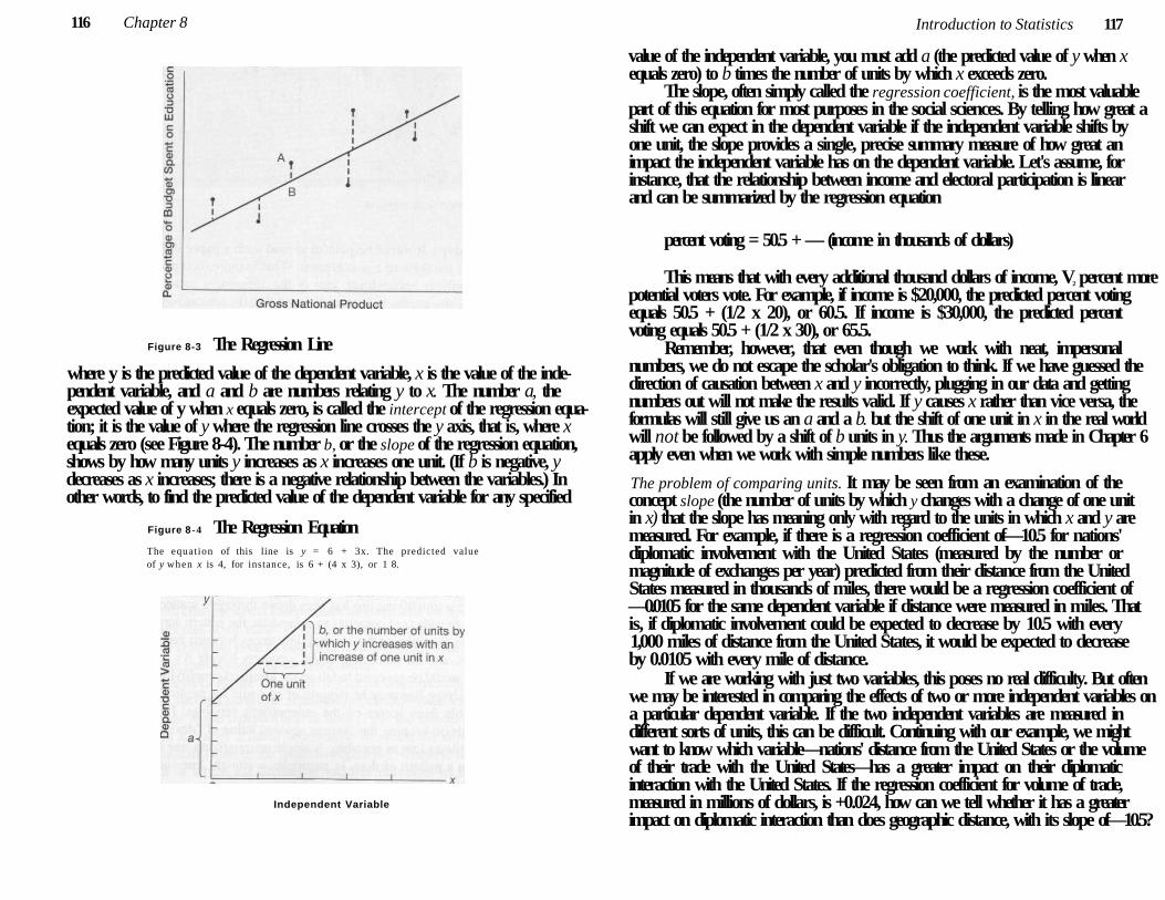
116 Chapter 8

Figure 8-3 The Regression Line

where y is the predicted value of the dependent variable, x is the value of the inde­pendent variable, and a and b are numbers relating y to x. The number a, the expected value of y when x equals zero, is called the intercept of the regression equa­tion; it is the value of y where the regression line crosses the y axis, that is, where x equals zero (see Figure 8-4). The number b, or the slope of the regression equation, shows by how many units y increases as x increases one unit. (If b is negative, y decreases as x increases; there is a negative relationship between the variables.) In other words, to find the predicted value of the dependent variable for any specified

Figure 8 -4 The Regression Equation The equat ion of this line is y = 6 + 3x. The predicted value of y when x is 4, for instance, is 6 + (4 x 3), or 1 8.

Independent Variable

Introduction to Statistics 117

value of the independent variable, you must add a (the predicted value of y when x equals zero) to b times the number of units by which x exceeds zero.

The slope, often simply called the regression coefficient, is the most valuable part of this equation for most purposes in the social sciences. By telling how great a shift we can expect in the dependent variable if the independent variable shifts by one unit, the slope provides a single, precise summary measure of how great an impact the independent variable has on the dependent variable. Let's assume, for instance, that the relationship between income and electoral participation is linear and can be summarized by the regression equation

percent voting = 50.5 + — (income in thousands of dollars)

This means that with every additional thousand dollars of income, V2 percent more potential voters vote. For example, if income is $20,000, the predicted percent voting equals 50.5 + (1/2 x 20), or 60.5. If income is $30,000, the predicted percent voting equals 50.5 + (1/2 x 30), or 65.5.

Remember, however, that even though we work with neat, impersonal numbers, we do not escape the scholar's obligation to think. If we have guessed the direction of causation between x and y incorrectly, plugging in our data and getting numbers out will not make the results valid. If y causes x rather than vice versa, the formulas will still give us an a and a b. but the shift of one unit in x in the real world will not be followed by a shift of b units in y. Thus the arguments made in Chapter 6 apply even when we work with simple numbers like these.

The problem of comparing units. It may be seen from an examination of the concept slope (the number of units by which y changes with a change of one unit in x) that the slope has meaning only with regard to the units in which x and y are measured. For example, if there is a regression coefficient of—10.5 for nations' diplomatic involvement with the United States (measured by the number or magnitude of exchanges per year) predicted from their distance from the United States measured in thousands of miles, there would be a regression coefficient of —0.0105 for the same dependent variable if distance were measured in miles. That is, if diplomatic involvement could be expected to decrease by 10.5 with every 1,000 miles of distance from the United States, it would be expected to decrease by 0.0105 with every mile of distance.

If we are working with just two variables, this poses no real difficulty. But often we may be interested in comparing the effects of two or more independent variables on a particular dependent variable. If the two independent variables are measured in different sorts of units, this can be difficult. Continuing with our example, we might want to know which variable—nations' distance from the United States or the volume of their trade with the United States—has a greater impact on their diplomatic interaction with the United States. If the regression coefficient for volume of trade, measured in millions of dollars, is +0.024, how can we tell whether it has a greater impact on diplomatic interaction than does geographic distance, with its slope of—10.5?

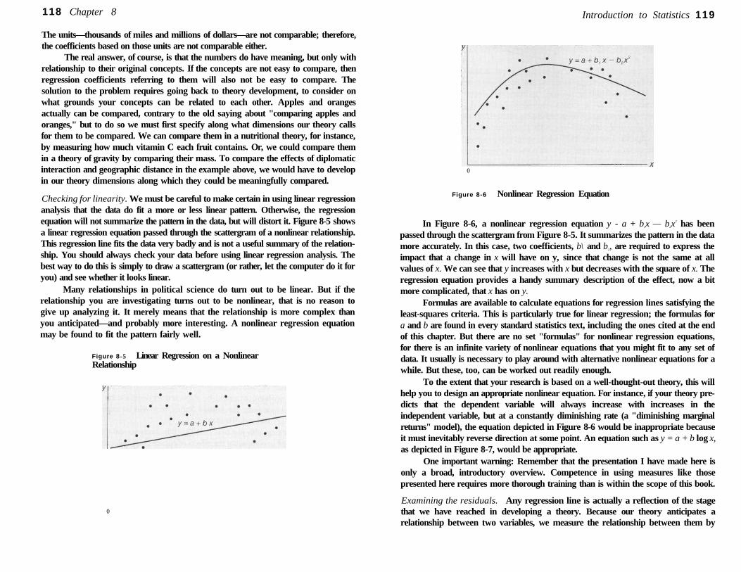
118 Chapter 8

The units—thousands of miles and millions of dollars—are not comparable; therefore, the coefficients based on those units are not comparable either.

The real answer, of course, is that the numbers do have meaning, but only with relationship to their original concepts. If the concepts are not easy to compare, then regression coefficients referring to them will also not be easy to compare. The solution to the problem requires going back to theory development, to consider on what grounds your concepts can be related to each other. Apples and oranges actually can be compared, contrary to the old saying about "comparing apples and oranges," but to do so we must first specify along what dimensions our theory calls for them to be compared. We can compare them in a nutritional theory, for instance, by measuring how much vitamin C each fruit contains. Or, we could compare them in a theory of gravity by comparing their mass. To compare the effects of diplomatic interaction and geographic distance in the example above, we would have to develop in our theory dimensions along which they could be meaningfully compared.

Checking for linearity. We must be careful to make certain in using linear regression analysis that the data do fit a more or less linear pattern. Otherwise, the regression equation will not summarize the pattern in the data, but will distort it. Figure 8-5 shows a linear regression equation passed through the scattergram of a nonlinear relationship. This regression line fits the data very badly and is not a useful summary of the relation­ship. You should always check your data before using linear regression analysis. The best way to do this is simply to draw a scattergram (or rather, let the computer do it for you) and see whether it looks linear.

Many relationships in political science do turn out to be linear. But if the relationship you are investigating turns out to be nonlinear, that is no reason to give up analyzing it. It merely means that the relationship is more complex than you anticipated—and probably more interesting. A nonlinear regression equation may be found to fit the pattern fairly well.

Figure 8-5 Linear Regression on a Nonlinear Relationship

0

Introduction to Statistics 119

0

Figure 8-6 Nonlinear Regression Equation

In Figure 8-6, a nonlinear regression equation y - a + bxx — b2x2 has been

passed through the scattergram from Figure 8-5. It summarizes the pattern in the data more accurately. In this case, two coefficients, b\ and b2, are required to express the impact that a change in x will have on y, since that change is not the same at all values of x. We can see that y increases with x but decreases with the square of x. The regression equation provides a handy summary description of the effect, now a bit more complicated, that x has on y.

Formulas are available to calculate equations for regression lines satisfying the least-squares criteria. This is particularly true for linear regression; the formulas for a and b are found in every standard statistics text, including the ones cited at the end of this chapter. But there are no set "formulas" for nonlinear regression equations, for there is an infinite variety of nonlinear equations that you might fit to any set of data. It usually is necessary to play around with alternative nonlinear equations for a while. But these, too, can be worked out readily enough.

To the extent that your research is based on a well-thought-out theory, this will help you to design an appropriate nonlinear equation. For instance, if your theory pre­dicts that the dependent variable will always increase with increases in the independent variable, but at a constantly diminishing rate (a "diminishing marginal returns" model), the equation depicted in Figure 8-6 would be inappropriate because it must inevitably reverse direction at some point. An equation such as y = a + b log x, as depicted in Figure 8-7, would be appropriate.

One important warning: Remember that the presentation I have made here is only a broad, introductory overview. Competence in using measures like those presented here requires more thorough training than is within the scope of this book.

Examining the residuals. Any regression line is actually a reflection of the stage that we have reached in developing a theory. Because our theory anticipates a relationship between two variables, we measure the relationship between them by

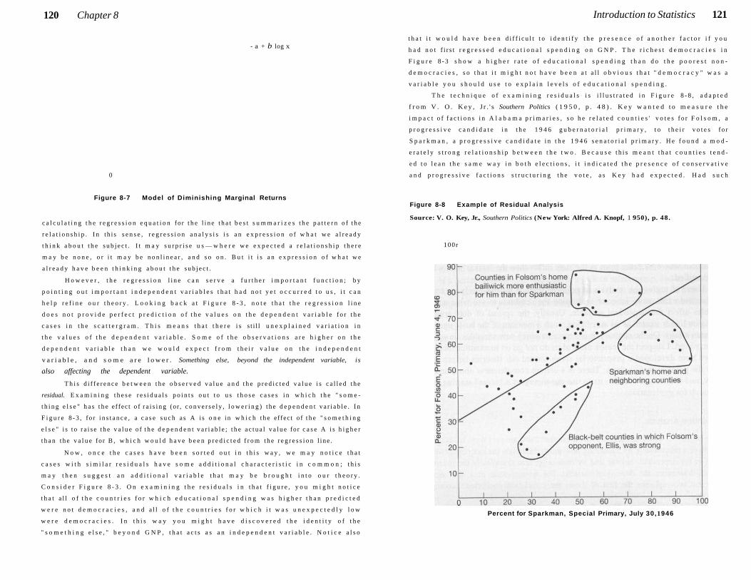
120 Chapter 8

- a + b log x

0

Figure 8-7 Model of Diminishing Marginal Returns

c a l c u l a t i n g t h e r e g r e s s i o n e q u a t i o n for t h e l i n e t h a t b e s t s u m m a r i z e s t h e p a t t e r n o f t h e

r e l a t i o n s h i p . I n t h i s s e n s e , r e g r e s s i o n a n a l y s i s i s a n e x p r e s s i o n o f w h a t w e a l r e a d y

t h i n k a b o u t t h e s u b j e c t . I t m a y s u r p r i s e u s — w h e r e w e e x p e c t e d a r e l a t i o n s h i p t h e r e

m a y b e n o n e , o r i t m a y b e n o n l i n e a r , a n d s o o n . B u t i t i s a n e x p r e s s i o n o f w h a t w e

a l r e a d y h a v e b e e n t h i n k i n g a b o u t t h e s u b j e c t .

H o w e v e r , t h e r e g r e s s i o n l i n e c a n s e r v e a f u r t h e r i m p o r t a n t f u n c t i o n ; b y

p o i n t i n g o u t i m p o r t a n t i n d e p e n d e n t v a r i a b l e s t h a t h a d n o t y e t o c c u r r e d t o u s , i t c a n

h e l p r e f i n e o u r t h e o r y . L o o k i n g b a c k a t F i g u r e 8 - 3 , n o t e t h a t t h e r e g r e s s i o n l i n e

d o e s n o t p r o v i d e p e r f e c t p r e d i c t i o n o f t h e v a l u e s o n t h e d e p e n d e n t v a r i a b l e f o r t h e

c a s e s i n t h e s c a t t e r g r a m . T h i s m e a n s t h a t t h e r e i s s t i l l u n e x p l a i n e d v a r i a t i o n i n

t h e v a l u e s o f t h e d e p e n d e n t v a r i a b l e . S o m e o f t h e o b s e r v a t i o n s a r e h i g h e r o n t h e

d e p e n d e n t v a r i a b l e t h a n w e w o u l d e x p e c t f r o m t h e i r v a l u e o n t h e i n d e p e n d e n t

v a r i a b l e , a n d s o m e a r e l o w e r . Something else, beyond the independent variable, is

also affecting the dependent variable.

T h i s d i f f e r e n c e b e t w e e n t h e o b s e r v e d v a l u e a n d t h e p r e d i c t e d v a l u e i s c a l l e d t h e

residual. E x a m i n i n g t h e s e r e s i d u a l s p o i n t s o u t t o u s t h o s e c a s e s i n w h i c h t h e " s o m e ­

t h i n g e l s e " h a s t h e ef fec t o f r a i s i n g (or , c o n v e r s e l y , l o w e r i n g ) t h e d e p e n d e n t v a r i a b l e . I n

F i g u r e 8 - 3 , fo r i n s t a n c e , a c a s e s u c h a s A i s o n e i n w h i c h t h e ef fec t o f t h e " s o m e t h i n g

e l s e " i s t o r a i s e t h e v a l u e o f t h e d e p e n d e n t v a r i a b l e ; t h e a c t u a l v a l u e for c a s e A i s h i g h e r

t h a n t h e v a l u e for B , w h i c h w o u l d h a v e b e e n p r e d i c t e d f r o m t h e r e g r e s s i o n l i n e .

N o w , o n c e t h e c a s e s h a v e b e e n s o r t e d o u t i n t h i s w a y , w e m a y n o t i c e t h a t

c a s e s w i t h s i m i l a r r e s i d u a l s h a v e s o m e a d d i t i o n a l c h a r a c t e r i s t i c i n c o m m o n ; t h i s

m a y t h e n s u g g e s t a n a d d i t i o n a l v a r i a b l e t h a t m a y b e b r o u g h t i n t o o u r t h e o r y .

C o n s i d e r F i g u r e 8 - 3 . O n e x a m i n i n g t h e r e s i d u a l s i n t h a t f i g u r e , y o u m i g h t n o t i c e

t h a t a l l o f t h e c o u n t r i e s f o r w h i c h e d u c a t i o n a l s p e n d i n g w a s h i g h e r t h a n p r e d i c t e d

w e r e n o t d e m o c r a c i e s , a n d a l l o f t h e c o u n t r i e s f o r w h i c h i t w a s u n e x p e c t e d l y l o w

w e r e d e m o c r a c i e s . I n t h i s w a y y o u m i g h t h a v e d i s c o v e r e d t h e i d e n t i t y o f t h e

" s o m e t h i n g e l s e , " b e y o n d G N P , t h a t a c t s a s a n i n d e p e n d e n t v a r i a b l e . N o t i c e a l s o

Introduction to Statistics 121

t h a t i t w o u l d h a v e b e e n d i f f i c u l t t o i d e n t i f y t h e p r e s e n c e o f a n o t h e r f a c t o r i f y o u

h a d n o t f i r s t r e g r e s s e d e d u c a t i o n a l s p e n d i n g o n G N P . T h e r i c h e s t d e m o c r a c i e s i n

F i g u r e 8 - 3 s h o w a h i g h e r r a t e o f e d u c a t i o n a l s p e n d i n g t h a n d o t h e p o o r e s t n o n -

d e m o c r a c i e s , s o t h a t i t m i g h t n o t h a v e b e e n a t a l l o b v i o u s t h a t " d e m o c r a c y " w a s a

v a r i a b l e y o u s h o u l d u s e t o e x p l a i n l e v e l s o f e d u c a t i o n a l s p e n d i n g .

T h e t e c h n i q u e o f e x a m i n i n g r e s i d u a l s i s i l l u s t r a t e d i n F i g u r e 8 - 8 , a d a p t e d

f r o m V . O . K e y , J r . ' s Southern Politics ( 1 9 5 0 , p . 4 8 ) . K e y w a n t e d t o m e a s u r e t h e

i m p a c t o f f a c t i o n s i n A l a b a m a p r i m a r i e s , s o h e r e l a t e d c o u n t i e s ' v o t e s f o r F o l s o m , a

p r o g r e s s i v e c a n d i d a t e i n t h e 1 9 4 6 g u b e r n a t o r i a l p r i m a r y , t o t h e i r v o t e s fo r

S p a r k m a n , a p r o g r e s s i v e c a n d i d a t e i n t h e 1 9 4 6 s e n a t o r i a l p r i m a r y . H e f o u n d a m o d ­

e r a t e l y s t r o n g r e l a t i o n s h i p b e t w e e n t h e t w o . B e c a u s e t h i s m e a n t t h a t c o u n t i e s t e n d ­

e d t o l e a n t h e s a m e w a y i n b o t h e l e c t i o n s , i t i n d i c a t e d t h e p r e s e n c e o f c o n s e r v a t i v e

a n d p r o g r e s s i v e f a c t i o n s s t r u c t u r i n g t h e v o t e , a s K e y h a d e x p e c t e d . H a d s u c h

Figure 8-8 Example of Residual Analysis

Source: V. O. Key, Jr., Southern Politics (New York: Alfred A. Knopf, 1 950), p. 48.

100r

Percent for Sparkman, Special Primary, July 30,1946

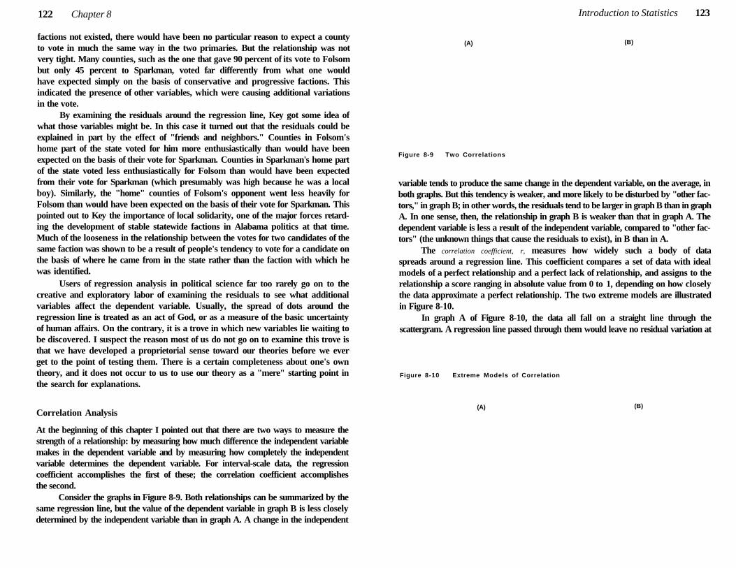
122 Chapter 8

factions not existed, there would have been no particular reason to expect a county to vote in much the same way in the two primaries. But the relationship was not very tight. Many counties, such as the one that gave 90 percent of its vote to Folsom but only 45 percent to Sparkman, voted far differently from what one would have expected simply on the basis of conservative and progressive factions. This indicated the presence of other variables, which were causing additional variations in the vote.

By examining the residuals around the regression line, Key got some idea of what those variables might be. In this case it turned out that the residuals could be explained in part by the effect of "friends and neighbors." Counties in Folsom's home part of the state voted for him more enthusiastically than would have been expected on the basis of their vote for Sparkman. Counties in Sparkman's home part of the state voted less enthusiastically for Folsom than would have been expected from their vote for Sparkman (which presumably was high because he was a local boy). Similarly, the "home" counties of Folsom's opponent went less heavily for Folsom than would have been expected on the basis of their vote for Sparkman. This pointed out to Key the importance of local solidarity, one of the major forces retard­ing the development of stable statewide factions in Alabama politics at that time. Much of the looseness in the relationship between the votes for two candidates of the same faction was shown to be a result of people's tendency to vote for a candidate on the basis of where he came from in the state rather than the faction with which he was identified.

Users of regression analysis in political science far too rarely go on to the creative and exploratory labor of examining the residuals to see what additional variables affect the dependent variable. Usually, the spread of dots around the regression line is treated as an act of God, or as a measure of the basic uncertainty of human affairs. On the contrary, it is a trove in which new variables lie waiting to be discovered. I suspect the reason most of us do not go on to examine this trove is that we have developed a proprietorial sense toward our theories before we ever get to the point of testing them. There is a certain completeness about one's own theory, and it does not occur to us to use our theory as a "mere" starting point in the search for explanations.

Correlation Analysis

At the beginning of this chapter I pointed out that there are two ways to measure the strength of a relationship: by measuring how much difference the independent variable makes in the dependent variable and by measuring how completely the independent variable determines the dependent variable. For interval-scale data, the regression coefficient accomplishes the first of these; the correlation coefficient accomplishes the second.

Consider the graphs in Figure 8-9. Both relationships can be summarized by the same regression line, but the value of the dependent variable in graph B is less closely determined by the independent variable than in graph A. A change in the independent

Introduction to Statistics 123

(A) (B)

Figure 8-9 Two Correlations

variable tends to produce the same change in the dependent variable, on the average, in both graphs. But this tendency is weaker, and more likely to be disturbed by "other fac­tors," in graph B; in other words, the residuals tend to be larger in graph B than in graph A. In one sense, then, the relationship in graph B is weaker than that in graph A. The dependent variable is less a result of the independent variable, compared to "other fac­tors" (the unknown things that cause the residuals to exist), in B than in A.

The correlation coefficient, r, measures how widely such a body of data spreads around a regression line. This coefficient compares a set of data with ideal models of a perfect relationship and a perfect lack of relationship, and assigns to the relationship a score ranging in absolute value from 0 to 1, depending on how closely the data approximate a perfect relationship. The two extreme models are illustrated in Figure 8-10.

In graph A of Figure 8-10, the data all fall on a straight line through the scattergram. A regression line passed through them would leave no residual variation at

Figure 8-10 Extreme Models of Correlation

(A) (B)

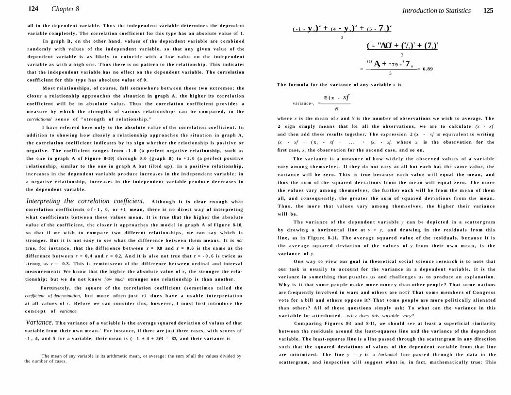
124 Chapter 8

all in the d e p e n d e n t variable . T h u s the i n d e p e n d e n t variable d e t e r m i n e s the d e p e n d e n t

var iable c o m p l e t e l y . T h e corre lat ion coef f i c i ent for this t y p e has an abso lu te v a l u e o f 1 .

I n g r a p h B , o n the o ther h a n d , v a l u e s o f the d e p e n d e n t var iab le are c o m b i n e d

r a n d o m l y w i t h v a l u e s o f the i n d e p e n d e n t var iab le , s o that a n y g i v e n v a l u e o f the

d e p e n d e n t var iab le i s a s l i k e l y t o c o i n c i d e w i t h a l o w v a l u e o n the i n d e p e n d e n t

var iab le a s w i t h a h i g h o n e . T h u s there i s no pattern to the re la t ionsh ip . T h i s i n d i c a t e s

that the i n d e p e n d e n t var iab le h a s n o e f f ec t o n the d e p e n d e n t var iable . T h e corre la t ion

c o e f f i c i e n t for this t y p e h a s a b s o l u t e v a l u e o f 0 .

M o s t r e l a t i o n s h i p s , o f c o u r s e , fal l s o m e w h e r e b e t w e e n t h e s e t w o e x t r e m e s ; the

c l o s e r a r e l a t i o n s h i p a p p r o a c h e s the s i tua t ion in g r a p h A , the h i g h e r i ts c o r r e l a t i o n

c o e f f i c i e n t w i l l b e i n a b s o l u t e v a l u e . T h u s the c o r r e l a t i o n c o e f f i c i e n t p r o v i d e s a

m e a s u r e b y w h i c h the s t r e n g t h s o f v a r i o u s r e l a t i o n s h i p s c a n b e c o m p a r e d , i n the

correlational s e n s e o f "s trength o f r e l a t i o n s h i p . "

I h a v e referred h e r e o n l y to the a b s o l u t e v a l u e o f the c o r r e l a t i o n c o e f f i c i e n t . In

a d d i t i o n t o s h o w i n g h o w c l o s e l y a r e l a t i o n s h i p a p p r o a c h e s the s i tua t ion i n g r a p h A ,

the c o r r e l a t i o n c o e f f i c i e n t i n d i c a t e s b y i ts s i g n w h e t h e r the r e l a t i o n s h i p i s p o s i t i v e o r

n e g a t i v e . T h e c o e f f i c i e n t r a n g e s f r o m - 1 . 0 ( a p e r f e c t n e g a t i v e r e l a t i o n s h i p , s u c h a s

the o n e i n g r a p h A o f F i g u r e 8-10) t h r o u g h 0 . 0 ( g r a p h B ) t o + 1 . 0 ( a p e r f e c t p o s i t i v e

r e l a t i o n s h i p , s i m i l a r to the o n e in g r a p h A but t i l t ed up) . In a p o s i t i v e r e l a t i o n s h i p ,

i n c r e a s e s i n the d e p e n d e n t v a r i a b l e p r o d u c e i n c r e a s e s i n the i n d e p e n d e n t var iab le ; i n

a n e g a t i v e r e l a t i o n s h i p , i n c r e a s e s i n the i n d e p e n d e n t v a r i a b l e p r o d u c e d e c r e a s e s i n

the d e p e n d e n t var iab l e .

Interpreting the correlation coefficient. A l t h o u g h it is c l e a r e n o u g h w h a t

c o r r e l a t i o n c o e f f i c i e n t s o f - 1 , 0 , o r + 1 m e a n , there i s n o d irec t w a y o f in terpre t ing

w h a t c o e f f i c i e n t s b e t w e e n t h e s e v a l u e s m e a n . I t i s true that the h i g h e r the a b s o l u t e

v a l u e o f the c o e f f i c i e n t , t h e c l o s e r i t a p p r o a c h e s the m o d e l in g r a p h A o f F i g u r e 8-10,

s o that i f w e w i s h t o c o m p a r e t w o d i f ferent r e l a t i o n s h i p s , w e c a n s a y w h i c h i s

s tronger . B u t i t i s n o t e a s y t o s e e w h a t the d i f f e r e n c e b e t w e e n t h e m m e a n s . I t i s not

true, for i n s t a n c e , that the d i f f e r e n c e b e t w e e n r = 0.8 and r = 0 . 6 is t h e s a m e as the

d i f f e r e n c e b e t w e e n r = 0 . 4 a n d r = 0.2. A n d it is a l s o no t true that r = - 0 . 6 is t w i c e as

s t rong as r = -0.3. T h i s i s r e m i n i s c e n t o f the d i f f e r e n c e b e t w e e n ord ina l a n d interva l

m e a s u r e m e n t : W e k n o w that t h e h i g h e r the a b s o l u t e v a l u e o f r , the s t r o n g e r the re la ­

t i o n s h i p ; but we do n o t k n o w how much s t r o n g e r o n e r e l a t i o n s h i p i s than another .

For tunate ly , the s q u a r e o f the c o r r e l a t i o n c o e f f i c i e n t ( s o m e t i m e s c a l l e d the

coefficient of determination, but m o r e o f t en j u s t r2) d o e s h a v e a u s a b l e in terpre ta t ion

a t al l v a l u e s o f r . B e f o r e we c a n c o n s i d e r th i s , h o w e v e r , I m u s t first i n t r o d u c e the

c o n c e p t of variance.

Variance. T h e var iance o f a variable is the average squared dev ia t i on o f v a l u e s o f that

variable f r o m their o w n m e a n . 1 For ins tance , i f there are jus t three c a s e s , w i t h s c o r e s o f

- 1 , 4, and 5 for a variable , their m e a n is (- 1 + 4 + 5)/3 = 8/3, and their var iance is

'The mean of any variable is its arithmetic mean, or average: the sum of all the values divided by the number of cases.

Introduction to Statistics 125

( - i - y 3)2 + ( 4 - y 3)

2 + (5 - 7 3)2

3

( - "AO2 + (4/3)2 + (73)

2

3 121 A, + " 7 9 +

4 7 9 = — = 6.89

3

T h e f o r m u l a for t h e v a r i a n c e o f a n y v a r i a b l e x i s

E ( x - xf variance-, =

N

w h e r e x i s the m e a n o f x a n d N i s the n u m b e r o f o b s e r v a t i o n s we w i s h to average . T h e

2 s i g n s i m p l y m e a n s that for all the o b s e r v a t i o n s , we are to c a l c u l a t e (x - xf

and then add t h e s e resu l t s together . T h e e x p r e s s i o n 2 (x - x f i s e q u i v a l e n t to wri t ing

(xx - xf + ( x 2 - xf + . . . + (xN - xf, w h e r e x x is the o b s e r v a t i o n for the

first c a s e , x 2 the o b s e r v a t i o n for the s e c o n d c a s e , and so on .

T h e v a r i a n c e i s a m e a s u r e o f h o w w i d e l y t h e o b s e r v e d v a l u e s o f a v a r i a b l e

v a r y a m o n g t h e m s e l v e s . I f t h e y d o n o t v a r y a t a l l b u t e a c h h a s t h e s a m e v a l u e , t h e

v a r i a n c e w i l l b e z e r o . T h i s i s t rue b e c a u s e e a c h v a l u e w i l l e q u a l t h e m e a n , a n d

t h u s t h e s u m o f t h e s q u a r e d d e v i a t i o n s f r o m t h e m e a n w i l l e q u a l z e r o . T h e m o r e

t h e v a l u e s v a r y a m o n g t h e m s e l v e s , t h e f u r t h e r e a c h w i l l b e f r o m t h e m e a n o f t h e m

a l l , a n d c o n s e q u e n t l y , t h e g r e a t e r t h e s u m o f s q u a r e d d e v i a t i o n s f r o m t h e m e a n .

T h u s , t h e m o r e that v a l u e s v a r y a m o n g t h e m s e l v e s , t h e h i g h e r t h e i r v a r i a n c e

w i l l b e .

T h e v a r i a n c e o f t h e d e p e n d e n t v a r i a b l e y c a n b e d e p i c t e d i n a s c a t t e r g r a m

by d r a w i n g a h o r i z o n t a l l i n e a t y = y , a n d d r a w i n g in t h e r e s i d u a l s f r o m t h i s

l i n e , a s i n F i g u r e 8-11. T h e a v e r a g e s q u a r e d v a l u e o f t h e r e s i d u a l s , b e c a u s e i t i s

t h e a v e r a g e s q u a r e d d e v i a t i o n o f t h e v a l u e s o f y f r o m t h e i r o w n m e a n , i s the

v a r i a n c e of y .

O n e w a y t o v i e w o u r g o a l i n t h e o r e t i c a l s o c i a l s c i e n c e r e s e a r c h i s t o n o t e that

our task i s u s u a l l y to a c c o u n t for the v a r i a n c e in a d e p e n d e n t var iab l e . I t i s the

v a r i a n c e i n s o m e t h i n g that p u z z l e s u s and c h a l l e n g e s u s t o p r o d u c e a n e x p l a n a t i o n .

W h y i s i t that s o m e p e o p l e m a k e m o r e m o n e y t h a n o ther p e o p l e ? T h a t s o m e n a t i o n s

are f r e q u e n t l y i n v o l v e d i n w a r s and o t h e r s are n o t ? T h a t s o m e m e m b e r s o f C o n g r e s s

v o t e for a b i l l a n d o t h e r s o p p o s e it? T h a t s o m e p e o p l e are m o r e p o l i t i c a l l y a l i e n a t e d

than o t h e r s ? A l l o f t h e s e q u e s t i o n s s i m p l y ask: T o w h a t c a n t h e v a r i a n c e i n this

v a r i a b l e be a t t r i b u t e d — w h y does this variable vary?

C o m p a r i n g F i g u r e s 8-3 and 8-11, we s h o u l d s e e at least a superf ic ia l s imi lar i ty

b e t w e e n the r e s i d u a l s a r o u n d the l eas t - squares l i n e a n d the v a r i a n c e o f the d e p e n d e n t

var iable . T h e l eas t - squares l ine i s a l ine p a s s e d through the scat tergram in any d irect ion

s u c h that the squared d e v i a t i o n s o f v a l u e s o f the d e p e n d e n t var iab le f r o m that l ine

are m i n i m i z e d . T h e l i n e y = y is a horizontal l i n e p a s s e d t h r o u g h the data in the

scat tergram, and i n s p e c t i o n w i l l s u g g e s t w h a t i s , i n fact , m a t h e m a t i c a l l y true: T h i s

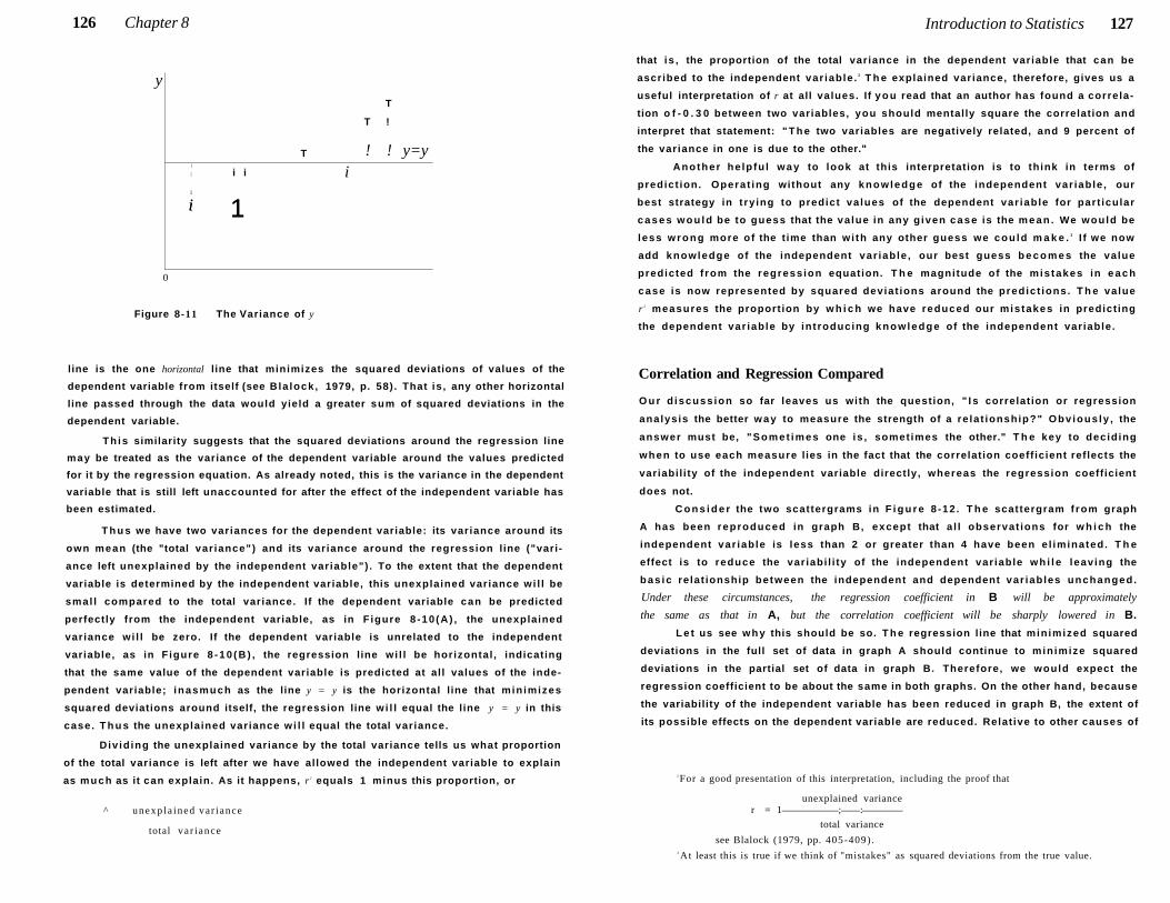
126 Chapter 8

y

T

T

T !

! ! y=y 1 1 i i i 1

i 1 1

i 1

0

Figure 8 -11 The Variance of y

l ine is the one horizontal l ine that minimizes the squared deviations of values of the

dependent variable from itself (see Bla lock , 1979, p. 58). That is , any other horizontal

line passed through the data would yield a greater sum of squared deviations in the

dependent variable.

Th is similarity suggests that the squared deviations around the regression line

may be treated as the variance of the dependent variable around the values predicted

for it by the regression equation. As already noted, this is the variance in the dependent

variable that is still left unaccounted for after the effect of the independent variable has

been estimated.

T h u s we have two variances for the dependent variable: its variance around its

own mean (the "total var iance") and its variance around the regression line ("vari­

ance left unexplained by the independent var iable") . To the extent that the dependent

variable is determined by the independent variable, this unexplained variance wi l l be

smal l compared to the total variance. If the dependent variable can be predicted

perfectly from the independent variable, as in F igure 8 -10 (A) , the unexplained

variance wi l l be zero. If the dependent variable is unrelated to the independent

variable, as in F igure 8 - 1 0 ( B ) , the regression line wi l l be horizontal , indicating

that the same value of the dependent variable is predicted at al l values of the inde­

pendent variable; inasmuch as the line y = y is the horizontal l ine that min imizes

squared deviations around itself, the regression line w i l l equal the l ine y = y in this

case. T h u s the unexplained variance w i l l equal the total variance.

D iv id ing the unexplained variance by the total variance tells us what proportion

of the total variance is left after we have al lowed the independent variable to explain

as much as it can explain. As it happens, r 2 equals 1 minus this proportion, or

^ unexp la ined va r iance

total va r i ance

Introduction to Statistics 127

that is , the proportion of the total variance in the dependent variable that can be

ascribed to the independent var iable . 2 T h e explained variance, therefore, gives us a

useful interpretation of r at all values. If y o u read that an author has found a correla­

tion o f - 0 . 3 0 between two variables, you should mentally square the correlation and

interpret that statement: " T h e two variables are negatively related, and 9 percent of

the variance in one is due to the other."

Another he lp fu l w a y to look at this interpretation is to think in terms of

predict ion. Operat ing without any knowledge of the independent var iable , our

best strategy in t ry ing to predict va lues of the dependent var iable for part icular

c a s e s w o u l d be to guess that the va lue in any g iven case is the m e a n . We would be

less w r o n g more of the t ime than wi th any other guess we cou ld m a k e . 3 I f we now

add knowledge of the independent var iable , our best guess b e c o m e s the value

predicted f rom the regress ion equation. T h e magnitude of the mis takes in e a c h

case is now represented by squared deviat ions around the predict ions. T h e value

r 2 measures the proport ion by w h i c h we have reduced our mistakes in predict ing

the dependent var iable by introducing knowledge of the independent var iable.

Correlation and Regression Compared

O u r d iscuss ion so far leaves us with the question, " I s correlat ion or regression

analysis the better w a y to measure the strength of a re lat ionship?" Obv ious ly , the

answer must be, "Somet imes one is , somet imes the other." T h e key to deciding

when to use each measure l ies in the fact that the correlation coeff icient reflects the

variabil i ty of the independent variable directly, whereas the regression coefficient

does not.

C o n s i d e r the two scattergrams in F i g u r e 8 -12 . T h e scattergram f rom graph

A has been reproduced in graph B, except that a l l observat ions for w h i c h the

independent var iable is less than 2 or greater than 4 have been e l iminated. T h e

effect is to reduce the var iabi l i ty of the independent var iable w h i l e leaving the

bas ic re lat ionship between the independent and dependent var iables unchanged.

Under these circumstances, the regression coefficient in B will be approximately

the same as that in A, but the correlation coefficient will be sharply lowered in B.

L e t us see w h y this should be so. T h e regression line that min imized squared

deviations in the full set of data in graph A should continue to min imize squared

deviations in the partial set of data in graph B. Therefore, we would expect the

regression coefficient to be about the same in both graphs. On the other hand, because

the variability of the independent variable has been reduced in graph B, the extent of

its possible effects on the dependent variable are reduced. Relat ive to other causes of

2 For a good presentation of this interpretation, including the proof that

unexplained variance r = 1 ; :

total variance

see Blalock (1979, pp. 405-409) . 3 At least this is true if we think of "mistakes" as squared deviations from the true value.

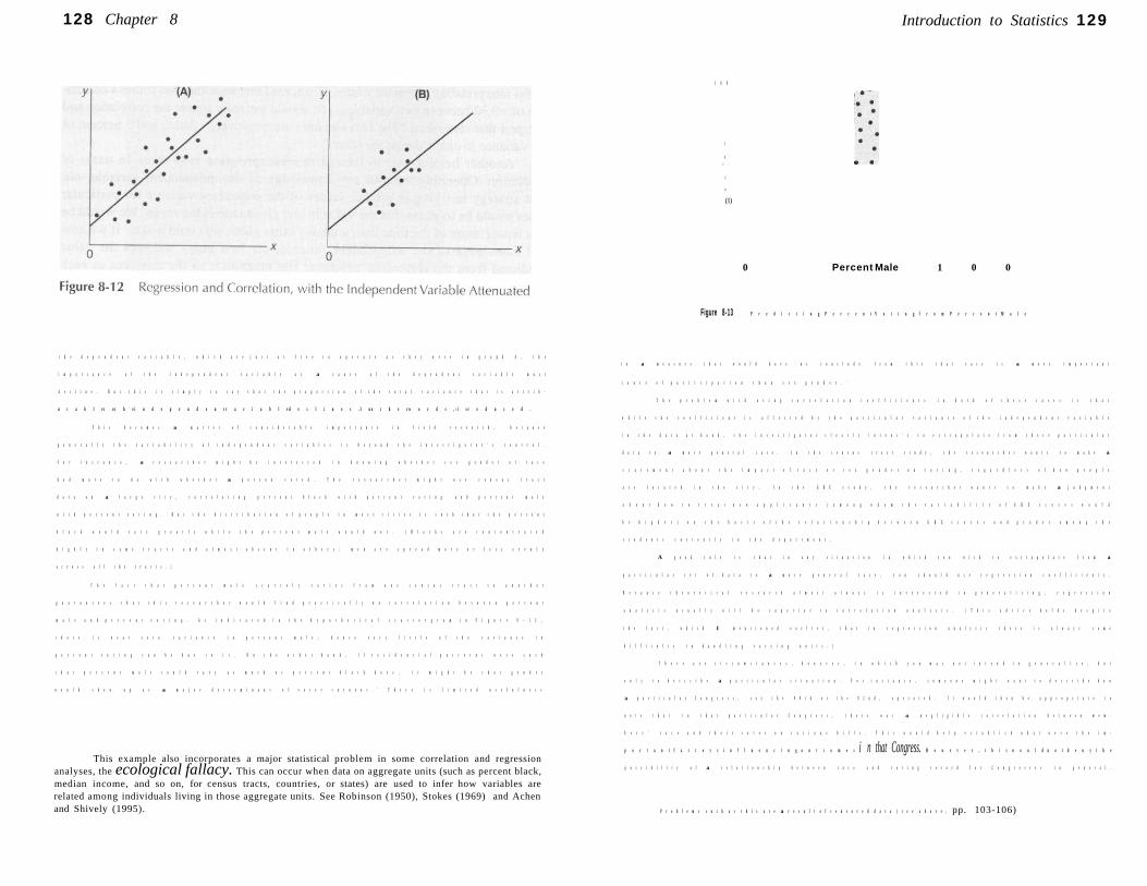
128 Chapter 8

t h e d e p e n d e n t v a r i a b l e , w h i c h a r e j u s t a s f r e e t o o p e r a t e a s t h e y w e r e i n g r a p h A , t h e

i m p o r t a n c e o f t h e i n d e p e n d e n t v a r i a b l e a s a c a u s e o f t h e d e p e n d e n t v a r i a b l e m u s t

d e c l i n e . B u t t h i s i s s i m p l y t o s a y t h a t t h e p r o p o r t i o n o f t h e t o t a l v a r i a n c e t h a t i s a t t r i b ­

u t a b l e t o t h e i n d e p e n d e n t v a r i a b l e d e c l i n e s . I n o t h e r w o r d s , r i s r e d u c e d .

T h i s b e c o m e s a m a t t e r o f c o n s i d e r a b l e i m p o r t a n c e i n f i e l d r e s e a r c h , b e c a u s e

g e n e r a l l y t h e v a r i a b i l i t y o f i n d e p e n d e n t v a r i a b l e s i s b e y o n d t h e i n v e s t i g a t o r ' s c o n t r o l .

F o r i n s t a n c e , a r e s e a r c h e r m i g h t b e i n t e r e s t e d i n k n o w i n g w h e t h e r s e x g e n d e r o r r a c e

h a d m o r e t o d o w i t h w h e t h e r a p e r s o n v o t e d . T h e r e s e a r c h e r m i g h t u s e c e n s u s t r a c t

d a t a o n a l a r g e c i t y , c o r r e l a t i n g p e r c e n t b l a c k w i t h p e r c e n t v o t i n g a n d p e r c e n t m a l e

w i t h p e r c e n t v o t i n g . B u t t h e d i s t r i b u t i o n o f p e o p l e i n m o s t c i t i e s i s s u c h t h a t t h e p e r c e n t

b l a c k w o u l d v a r y g r e a t l y w h i l e t h e p e r c e n t m a l e w o u l d n o t . ( B l a c k s a r e c o n c e n t r a t e d

h i g h l y i n s o m e t r a c t s a n d a l m o s t a b s e n t i n o t h e r s ; m e n a r e s p r e a d m o r e o r l e s s e v e n l y

a c r o s s a l l t h e t r a c t s . )

T h e f a c t t h a t p e r c e n t m a l e s c a r c e l y v a r i e s f r o m o n e c e n s u s t r a c t t o a n o t h e r

g u a r a n t e e s t h a t t h i s r e s e a r c h e r w o u l d f i n d p r a c t i c a l l y n o c o r r e l a t i o n b e t w e e n p e r c e n t

m a l e a n d p e r c e n t v o t i n g . A s i n d i c a t e d i n t h e h y p o t h e t i c a l s c a t t e r g r a m i n F i g u r e 8 - 1 3 ,

t h e r e i s n e a r z e r o v a r i a n c e i n p e r c e n t m a l e ; h e n c e v e r y l i t t l e o f t h e v a r i a n c e i n

p e r c e n t v o t i n g c a n b e d u e t o i t . O n t h e o t h e r h a n d , i f r e s i d e n t i a l p a t t e r n s w e r e s u c h

t h a t p e r c e n t m a l e c o u l d v a r y a s m u c h a s p e r c e n t b l a c k d o e s , i t m i g h t b e t h a t g e n d e r

w o u l d s h o w u p a s a m a j o r d e t e r m i n a n t o f v o t e r t u r n o u t . 4 T h e r e i s l i m i t e d u s e f u l n e s s

This example also incorporates a major statistical problem in some correlation and regression analyses, the ecological fallacy. This can occur when data on aggregate units (such as percent black, median income, and so on, for census tracts, countries, or states) are used to infer how variables are related among individuals living in those aggregate units. See Robinson (1950), Stokes (1969) and Achen and Shively (1995).

Introduction to Statistics 129

1 0 0

c

o >

c

o

(1)

0 Percent Male 1 0 0

Figure 8-13 P r e d i c t i n g P e r c e n t V o t i n g f r o m P e r c e n t M a l e

t o a m e a s u r e t h a t w o u l d h a v e u s c o n c l u d e f r o m t h i s t h a t r a c e i s a m o r e i m p o r t a n t

c a u s e o f p a r t i c i p a t i o n t h a n s e x g e n d e r . 5

T h e p r o b l e m w i t h u s i n g c o r r e l a t i o n c o e f f i c i e n t s i n b o t h o f t h e s e c a s e s i s t h a t

w h i l e t h e c o e f f i c i e n t i s a f f e c t e d b y t h e p a r t i c u l a r v a r i a n c e o f t h e i n d e p e n d e n t v a r i a b l e

i n t h e d a t a a t h a n d , t h e i n v e s t i g a t o r c l e a r l y i n t e n c ' s t o e x t r a p o l a t e f r o m t h e s e p a r t i c u l a r

d a t a t o a m o r e g e n e r a l c a s e . I n t h e c e n s u s t r a c t s t u d y , t h e r e s e a r c h e r w a n t s t o m a k e a

s t a t e m e n t a b o u t t h e i m p a c t o f r a c e o r s e x g e n d e r o n v o t i n g , r e g a r d l e s s o f h o w p e o p l e

a r e l o c a t e d i n t h e c i t y . I n t h e G R E s t u d y , t h e r e s e a r c h e r w a n t s t o m a k e a j u d g m e n t

a b o u t h o w t o t r e a t n e w a p p l i c a n t s ( a m o n g w h o m t h e v a r i a b i l i t y o f G R E s c o r e s w o u l d

b e h i g h e r ) o n t h e b a s i s o f t h e r e l a t i o n s h i p b e t w e e n G R E s c o r e s a n d g r a d e s a m o n g t h e

s t u d e n t s c u r r e n t l y i n t h e d e p a r t m e n t .

A g o o d r u l e i s t h a t i n a n y s i t u a t i o n i n w h i c h y o u w i s h t o e x t r a p o l a t e f r o m a

p a r t i c u l a r s e t o f d a t a t o a m o r e g e n e r a l c a s e , y o u s h o u l d u s e r e g r e s s i o n c o e f f i c i e n t s .

B e c a u s e t h e o r e t i c a l r e s e a r c h a l m o s t a l w a y s i s i n t e r e s t e d i n g e n e r a l i z i n g , r e g r e s s i o n

a n a l y s i s u s u a l l y w i l l b e s u p e r i o r t o c o r r e l a t i o n a n a l y s i s . ( T h i s a d v i c e h o l d s d e s p i t e

t h e f a c t , w h i c h I m e n t i o n e d e a r l i e r , t h a t i n r e g r e s s i o n a n a l y s i s t h e r e i s a l w a y s s o m e

d i f f i c u l t y i n h a n d l i n g v a r y i n g u n i t s . )

T h e r e a r e c i r c u m s t a n c e s , h o w e v e r , i n w h i c h y o u m a y n o t i n t e n d t o g e n e r a l i z e , b u t

o n l y t o d e s c r i b e a p a r t i c u l a r s i t u a t i o n . F o r i n s t a n c e , s o m e o n e m i g h t w a n t t o d e s c r i b e h o w

a p a r t i c u l a r C o n g r e s s , s a y t h e 8 0 t h o r t h e 9 2 n d , o p e r a t e d . I t w o u l d t h e n b e a p p r o p r i a t e t o

n o t e t h a t i n t h a t p a r t i c u l a r C o n g r e s s , t h e r e w a s a n e g l i g i b l e c o r r e l a t i o n b e t w e e n m e m ­

b e r s ' r a c e a n d t h e i r v o t e s o n v a r i o u s b i l l s . T h i s w o u l d h e l p e s t a b l i s h w h a t w e r e t h e i m ­

p o r t a n t f a c t o r s i n f l u e n c i n g o u t c o m e s i n that Congress. H o w e v e r , t h i s w o u l d n o t d e n y t h e

p o s s i b i l i t y o f a r e l a t i o n s h i p b e t w e e n r a c e a n d v o t i n g r e c o r d f o r C o n g r e s s e s i n g e n e r a l .

P r o b l e m s s u c h a s t h i s a r e a r e s u l t o f c e n s o r e d d a t a ( s e e a b o v e , pp. 103-106)

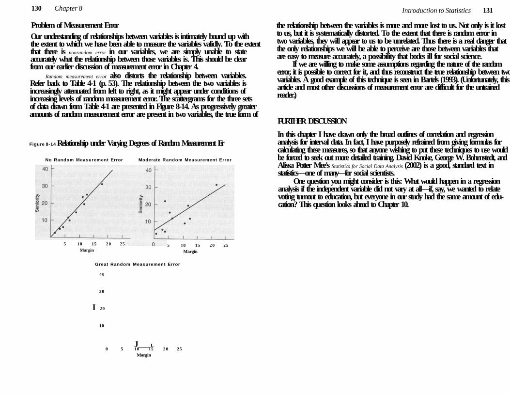
130 Chapter 8

Problem of Measurement Error Our understanding of relationships between variables is intimately bound up with the extent to which we have been able to measure the variables validly. To the extent that there is nonrandom error in our variables, we are simply unable to state accurately what the relationship between those variables is. This should be clear from our earlier discussion of measurement error in Chapter 4.

Random measurement error also distorts the relationship between variables. Refer back to Table 4-1 (p. 53). The relationship between the two variables is increasingly attenuated from left to right, as it might appear under conditions of increasing levels of random measurement error. The scattergrams for the three sets of data drawn from Table 4-1 are presented in Figure 8-14. As progressively greater amounts of random measurement error are present in two variables, the true form of

Figure 8-14 Relationship under Varying Degrees of Random Measurement Er

No Random Measurement Error Moderate Random Measurement Error

5 10 15 20 25 Margin

5 10 15 2 0 25 Margin

Great Random Measurement Error

40

30

I 20

10

J L 0 5 10 15 20 25

Margin

Introduction to Statistics 131

the relationship between the variables is more and more lost to us. Not only is it lost to us, but it is systematically distorted. To the extent that there is random error in two variables, they will appear to us to be unrelated. Thus there is a real danger that the only relationships we will be able to perceive are those between variables that are easy to measure accurately, a possibility that bodes ill for social science.

If we are willing to make some assumptions regarding the nature of the random error, it is possible to correct for it, and thus reconstruct the true relationship between two variables. A good example of this technique is seen in Bartels (1993). (Unfortunately, this article and most other discussions of measurement error are difficult for the untrained reader.)

FURTHER DISCUSSION

In this chapter I have drawn only the broad outlines of correlation and regression analysis for interval data. In fact, I have purposely refrained from giving formulas for calculating these measures, so that anyone wishing to put these techniques to use would be forced to seek out more detailed training. David Knoke, George W. Bohrnstedt, and Alissa Potter Mee's Statistics for Social Data Analysis (2002) is a good, standard text in statistics—one of many—for social scientists.

One question you might consider is this: What would happen in a regression analysis if the independent variable did not vary at all—if, say, we wanted to relate voting turnout to education, but everyone in our study had the same amount of edu­cation? This question looks ahead to Chapter 10.

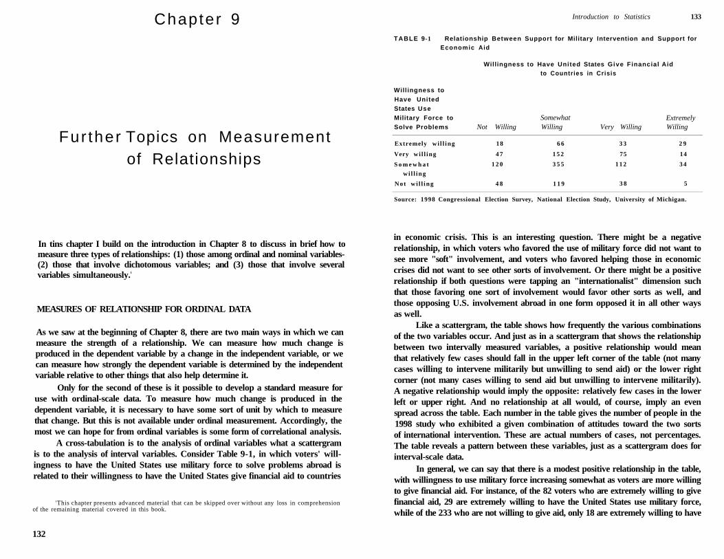
Chapter 9

Fur ther Topics on Measurement of Relationships

In tins chapter I build on the introduction in Chapter 8 to discuss in brief how to measure three types of relationships: (1) those among ordinal and nominal variables-(2) those that involve dichotomous variables; and (3) those that involve several variables simultaneously.1

MEASURES OF RELATIONSHIP FOR ORDINAL DATA

As we saw at the beginning of Chapter 8, there are two main ways in which we can measure the strength of a relationship. We can measure how much change is produced in the dependent variable by a change in the independent variable, or we can measure how strongly the dependent variable is determined by the independent variable relative to other things that also help determine it.

Only for the second of these is it possible to develop a standard measure for use with ordinal-scale data. To measure how much change is produced in the dependent variable, it is necessary to have some sort of unit by which to measure that change. But this is not available under ordinal measurement. Accordingly, the most we can hope for from ordinal variables is some form of correlational analysis.

A cross-tabulation is to the analysis of ordinal variables what a scattergram is to the analysis of interval variables. Consider Table 9-1, in which voters' will­ingness to have the United States use military force to solve problems abroad is related to their willingness to have the United States give financial aid to countries

'This chapter presents advanced material that can be skipped over without any loss in comprehension of the remaining material covered in this book.

132

Introduction to Statistics 133

TABLE 9-1 Relationship Between Support for Military Intervention and Support for Economic Aid

Willingness to Have United States Give Financial Aid to Countries in Crisis

Will ingness to Have United States Use Military Force to Somewhat Extremely Solve Problems Not Willing Willing Very Willing Willing

Extremely wi l l ing 18 6 6 3 3 2 9

Very wi l l ing 4 7 1 5 2 75 14

S o m e w h a t 1 2 0 3 5 5 1 1 2 3 4

w i l l ing

N o t w i l l ing 4 8 1 1 9 3 8 5

Source: 1998 Congressional Election Survey, National Election Study, University of Michigan.

in economic crisis. This is an interesting question. There might be a negative relationship, in which voters who favored the use of military force did not want to see more "soft" involvement, and voters who favored helping those in economic crises did not want to see other sorts of involvement. Or there might be a positive relationship if both questions were tapping an "internationalist" dimension such that those favoring one sort of involvement would favor other sorts as well, and those opposing U.S. involvement abroad in one form opposed it in all other ways as well.

Like a scattergram, the table shows how frequently the various combinations of the two variables occur. And just as in a scattergram that shows the relationship between two intervally measured variables, a positive relationship would mean that relatively few cases should fall in the upper left corner of the table (not many cases willing to intervene militarily but unwilling to send aid) or the lower right corner (not many cases willing to send aid but unwilling to intervene militarily). A negative relationship would imply the opposite: relatively few cases in the lower left or upper right. And no relationship at all would, of course, imply an even spread across the table. Each number in the table gives the number of people in the 1998 study who exhibited a given combination of attitudes toward the two sorts of international intervention. These are actual numbers of cases, not percentages. The table reveals a pattern between these variables, just as a scattergram does for interval-scale data.

In general, we can say that there is a modest positive relationship in the table, with willingness to use military force increasing somewhat as voters are more willing to give financial aid. For instance, of the 82 voters who are extremely willing to give financial aid, 29 are extremely willing to have the United States use military force, while of the 233 who are not willing to give aid, only 18 are extremely willing to have

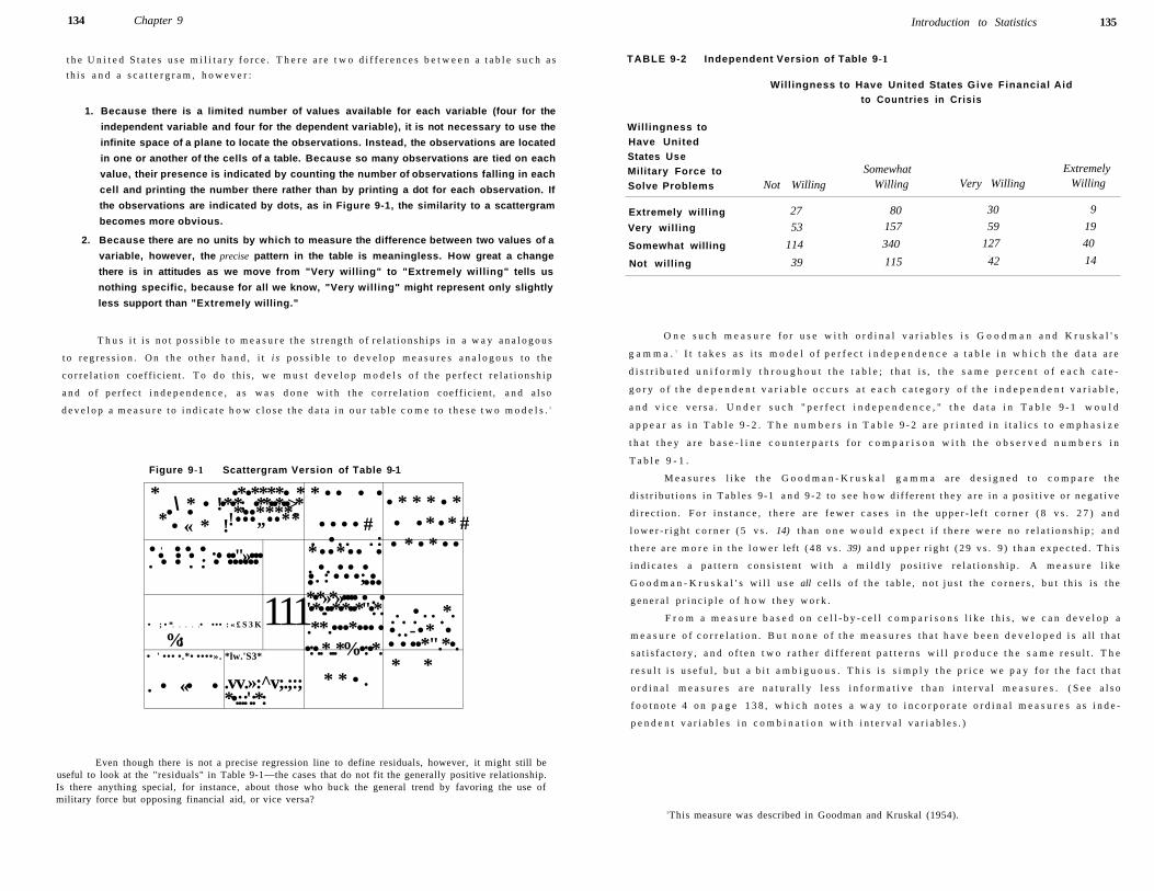
134 Chapter 9

t h e U n i t e d S t a t e s u s e m i l i t a r y f o r c e . T h e r e a r e t w o d i f f e r e n c e s b e t w e e n a t a b l e s u c h a s

t h i s a n d a s c a t t e r g r a m , h o w e v e r :

1. Because there is a limited number of values available for each variable (four for the

independent variable and four for the dependent variable), it is not necessary to use the

infinite space of a plane to locate the observations. Instead, the observations are located

in one or another of the cells of a table. Because so many observations are tied on each

value, their presence is indicated by counting the number of observations falling in each

cell and printing the number there rather than by printing a dot for each observation. If

the observations are indicated by dots, as in Figure 9-1, the similarity to a scattergram

becomes more obvious.

2. Because there are no units by which to measure the difference between two values of a

variable, however, the precise pattern in the table is meaningless. How great a change

there is in attitudes as we move from "Very willing" to "Extremely willing" tells us

nothing specific, because for all we know, "Very willing" might represent only slightly

less support than "Extremely willing."

T h u s i t i s n o t p o s s i b l e t o m e a s u r e t h e s t r e n g t h o f r e l a t i o n s h i p s i n a w a y a n a l o g o u s

t o r e g r e s s i o n . O n t h e o t h e r h a n d , i t i s p o s s i b l e t o d e v e l o p m e a s u r e s a n a l o g o u s t o t h e

c o r r e l a t i o n coef f ic ien t . T o d o th i s , w e m u s t d e v e l o p m o d e l s o f t h e p e r f e c t r e l a t i o n s h i p

a n d o f p e r f e c t i n d e p e n d e n c e , a s w a s d o n e w i t h t h e c o r r e l a t i o n coef f ic ien t , a n d a l s o

d e v e l o p a m e a s u r e t o i n d i c a t e h o w c l o s e t h e d a t a i n o u r t a b l e c o m e t o t h e s e t w o m o d e l s . 2

Figure 9-1 Scattergram Version of Table 9-1

* •*•****• * \ * • !•*•*; •**••*••>* • • *••****-* !•••„••** • « * !

* • • • •

• • • • # . • . . . :

• * * * • * • • * • * # • * • * • • • ' • • • .. • • • . • ••"»••• . • • . . • •••••• *••*•• •

. •. • • • •. : • • •; • • •••

• ; • * • ••• : « £ S 3 K

%: • ' ••• •.*• ••••». *lw.'S3*

111 *•*»*»•••• • . • '•*•..••*•*••*"•.*. .**.•••*••• • •:•..*...*%•:•*.

. • . . *. . . . . •..-•* • • • ••*".*•.

. • «• • .vv.»:̂ v;.;:; *•.:.:'.:*:

* * • . * *

Even though there is not a precise regression line to define residuals, however, it might still be useful to look at the "residuals" in Table 9-1—the cases that do not fit the generally positive relationship. Is there anything special, for instance, about those who buck the general trend by favoring the use of military force but opposing financial aid, or vice versa?

Introduction to Statistics 135

Willingness to Have United States Use Military Force to Solve Problems Not Willing

Somewhat Willing Very Willing

Extremely Willing

Extremely willing 27 80 30 9

Very willing 53 157 59 19

Somewhat willing 114 340 127 40

Not willing 39 115 42 14

O n e s u c h m e a s u r e f o r u s e w i t h o r d i n a l v a r i a b l e s i s G o o d m a n a n d K r u s k a l ' s

g a m m a . 3 I t t a k e s a s i t s m o d e l o f p e r f e c t i n d e p e n d e n c e a t a b l e i n w h i c h t h e d a t a a r e

d i s t r i b u t e d u n i f o r m l y t h r o u g h o u t t h e t a b l e ; t h a t i s , t h e s a m e p e r c e n t o f e a c h c a t e ­

g o r y o f t h e d e p e n d e n t v a r i a b l e o c c u r s a t e a c h c a t e g o r y o f t h e i n d e p e n d e n t v a r i a b l e ,

a n d v i c e v e r s a . U n d e r s u c h " p e r f e c t i n d e p e n d e n c e , " t h e d a t a i n T a b l e 9 - 1 w o u l d

a p p e a r a s i n T a b l e 9 - 2 . T h e n u m b e r s i n T a b l e 9 - 2 a r e p r i n t e d i n i t a l i c s t o e m p h a s i z e

t h a t t h e y a r e b a s e - l i n e c o u n t e r p a r t s f o r c o m p a r i s o n w i t h t h e o b s e r v e d n u m b e r s i n

T a b l e 9 - 1 .

M e a s u r e s l i k e t h e G o o d m a n - K r u s k a l g a m m a a r e d e s i g n e d t o c o m p a r e t h e

d i s t r i b u t i o n s i n T a b l e s 9 -1 a n d 9 - 2 t o s e e h o w d i f f e ren t t h e y a r e i n a p o s i t i v e o r n e g a t i v e

d i r e c t i o n . F o r i n s t a n c e , t h e r e a r e f e w e r c a s e s i n t h e u p p e r - l e f t c o r n e r ( 8 v s . 2 7 ) a n d

l o w e r - r i g h t c o r n e r ( 5 v s . 14) t h a n o n e w o u l d e x p e c t i f t h e r e w e r e n o r e l a t i o n s h i p ; a n d

t h e r e a r e m o r e i n t h e l o w e r left ( 4 8 v s . 39) a n d u p p e r r i g h t ( 2 9 v s . 9 ) t h a n e x p e c t e d . T h i s

i n d i c a t e s a p a t t e r n c o n s i s t e n t w i t h a m i l d l y p o s i t i v e r e l a t i o n s h i p . A m e a s u r e l i k e

G o o d m a n - K r u s k a l ' s w i l l u s e all c e l l s o f t h e t a b l e , n o t j u s t t h e c o r n e r s , b u t t h i s i s t h e

g e n e r a l p r i n c i p l e o f h o w t h e y w o r k .

F r o m a m e a s u r e b a s e d o n c e l l - b y - c e l l c o m p a r i s o n s l i k e t h i s , w e c a n d e v e l o p a

m e a s u r e o f c o r r e l a t i o n . B u t n o n e o f t h e m e a s u r e s t h a t h a v e b e e n d e v e l o p e d i s a l l t h a t

s a t i s f a c t o r y , a n d o f t e n t w o r a t h e r d i f f e r e n t p a t t e r n s w i l l p r o d u c e t h e s a m e r e s u l t . T h e

r e s u l t i s u s e f u l , b u t a b i t a m b i g u o u s . T h i s i s s i m p l y t h e p r i c e w e p a y f o r t h e f a c t t h a t

o r d i n a l m e a s u r e s a r e n a t u r a l l y l e s s i n f o r m a t i v e t h a n i n t e r v a l m e a s u r e s . ( S e e a l s o

f o o t n o t e 4 o n p a g e 1 3 8 , w h i c h n o t e s a w a y t o i n c o r p o r a t e o r d i n a l m e a s u r e s a s i n d e ­

p e n d e n t v a r i a b l e s i n c o m b i n a t i o n w i t h i n t e r v a l v a r i a b l e s . )

3 This measure was described in Goodman and Kruskal (1954).

TABLE 9-2 Independent Version of Table 9-1

Willingness to Have United States Give Financial Aid to Countries in Crisis

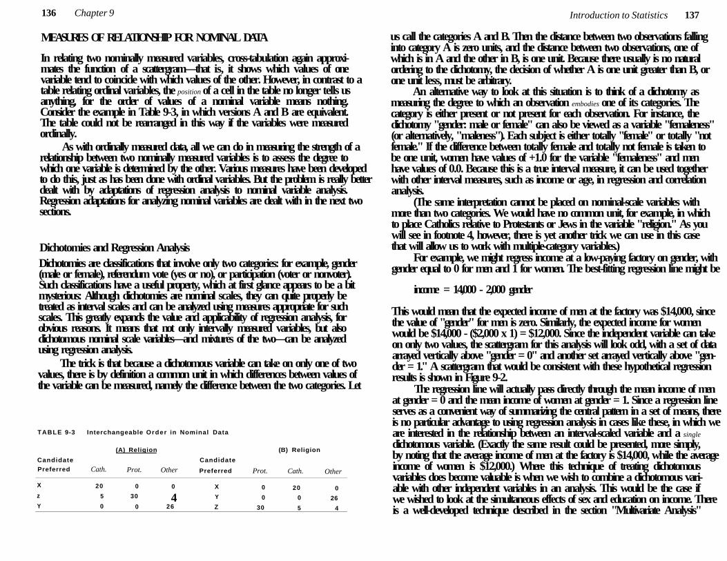
136 Chapter 9

MEASURES OF RELATIONSHIP FOR NOMINAL DATA

In relating two nominally measured variables, cross-tabulation again approxi­mates the function of a scattergram—that is, it shows which values of one variable tend to coincide with which values of the other. However, in contrast to a table relating ordinal variables, the position of a cell in the table no longer tells us anything, for the order of values of a nominal variable means nothing. Consider the example in Table 9-3, in which versions A and B are equivalent. The table could not be rearranged in this way if the variables were measured ordinally.

As with ordinally measured data, all we can do in measuring the strength of a relationship between two nominally measured variables is to assess the degree to which one variable is determined by the other. Various measures have been developed to do this, just as has been done with ordinal variables. But the problem is really better dealt with by adaptations of regression analysis to nominal variable analysis. Regression adaptations for analyzing nominal variables are dealt with in the next two sections.

Dichotomies and Regression Analysis Dichotomies are classifications that involve only two categories: for example, gender (male or female), referendum vote (yes or no), or participation (voter or nonvoter). Such classifications have a useful property, which at first glance appears to be a bit mysterious: Although dichotomies are nominal scales, they can quite properly be treated as interval scales and can be analyzed using measures appropriate for such scales. This greatly expands the value and applicability of regression analysis, for obvious reasons. It means that not only intervally measured variables, but also dichotomous nominal scale variables—and mixtures of the two—can be analyzed using regression analysis.

The trick is that because a dichotomous variable can take on only one of two values, there is by definition a common unit in which differences between values of the variable can be measured, namely the difference between the two categories. Let

TABLE 9-3 Interchangeable Order in Nominal Data

(A) Religion (B) Religion

Candidate Candidate Preferred Cath. Prot. Other Preferred Prot. Cath. Other

X 20 0 0 X 0 20 0 z 5 30 4 Y 0 0 26 Y 0 0 26 Z 30 5 4

Introduction to Statistics 137

us call the categories A and B. Then the distance between two observations falling into category A is zero units, and the distance between two observations, one of which is in A and the other in B, is one unit. Because there usually is no natural ordering to the dichotomy, the decision of whether A is one unit greater than B, or one unit less, must be arbitrary.

An alternative way to look at this situation is to think of a dichotomy as measuring the degree to which an observation embodies one of its categories. The category is either present or not present for each observation. For instance, the dichotomy "gender: male or female" can also be viewed as a variable "femaleness" (or alternatively, "maleness"). Each subject is either totally "female" or totally "not female." If the difference between totally female and totally not female is taken to be one unit, women have values of +1.0 for the variable "femaleness" and men have values of 0.0. Because this is a true interval measure, it can be used together with other interval measures, such as income or age, in regression and correlation analysis.

(The same interpretation cannot be placed on nominal-scale variables with more than two categories. We would have no common unit, for example, in which to place Catholics relative to Protestants or Jews in the variable "religion." As you will see in footnote 4, however, there is yet another trick we can use in this case that will allow us to work with multiple-category variables.)

For example, we might regress income at a low-paying factory on gender, with gender equal to 0 for men and 1 for women. The best-fitting regression line might be

income = 14,000 - 2,000 gender

This would mean that the expected income of men at the factory was $14,000, since the value of "gender" for men is zero. Similarly, the expected income for women would be $14,000 - ($2,000 x 1) = $12,000. Since the independent variable can take on only two values, the scattergram for this analysis will look odd, with a set of data arrayed vertically above "gender = 0" and another set arrayed vertically above "gen­der = 1." A scattergram that would be consistent with these hypothetical regression results is shown in Figure 9-2.

The regression line will actually pass directly through the mean income of men at gender = 0 and the mean income of women at gender = 1. Since a regression line serves as a convenient way of summarizing the central pattern in a set of means, there is no particular advantage to using regression analysis in cases like these, in which we are interested in the relationship between an interval-scaled variable and a single

dichotomous variable. (Exactly the same result could be presented, more simply, by noting that the average income of men at the factory is $14,000, while the average income of women is $12,000.) Where this technique of treating dichotomous variables does become valuable is when we wish to combine a dichotomous vari­able with other independent variables in an analysis. This would be the case if we wished to look at the simultaneous effects of sex and education on income. There is a well-developed technique described in the section "Multivariate Analysis"

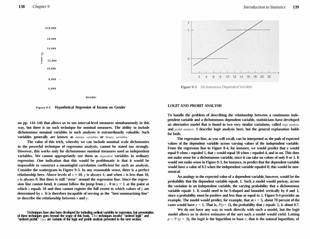
138 Chapter 9

$18 ,000

16 ,000

14 ,000

0 £ 8 12 ,000 c

10 ,000

8 ,000 -

6 ,000

Gender

Figure 9-2 Hypothetical Regression of Income on Gender

on pp. 141-146 that allows us to use interval-level measures simultaneously in this way, but there is no such technique for nominal measures. The ability to include dichotomous nominal variables in such analyses is extraordinarily valuable. Such variables generally are known as dummy variables or binary variables.4

The value of this trick, whereby we can include nominal scale dichotomies in the powerful technique of regression analysis, cannot be stated too strongly. However, this works only for dichotomous nominal measures used as independent variables. We cannot appropriately use them as dependent variables in ordinary regression. One indication that this would be problematic is that it would be impossible to construct a meaningful correlation coefficient for such an analysis. Consider the scattergram in Figure 9-3. In any reasonable sense, there is a perfect relationship here. Above levels of x = 10, y is always 1; and when x is less than 10, y is always 0. But there is still "error" around the regression line. Since the regres­sion line cannot bend, it cannot follow the jump from y - 0 to y = 1 at the point at which x equals 10 and thus cannot register the full extent to which values of y are determined by x. It is therefore incapable of serving as the "best summarizing line" to describe the relationship between x and y.

Techniques have also been developed for including ordinal variables in regression, but presentation of these techniques goes beyond the scope of this book. The techniques involve "ordered logit" and "ordered probit." They are variants of the logit and probit analysis presented in the next section.

Introduction to Statistics 139

LOGIT AND PROBIT ANALYSIS

To handle the problem of describing the relationship between a continuous inde­pendent variable and a dichotomous dependent variable, statisticians have developed an alternative model that is found in two very similar variations, called logit analysis

and probit analysis. I describe logit analysis here, but the general explanation holds for both.

The regression line, as you will recall, can be interpreted as the path of expected values of the dependent variable across varying values of the independent variable. From the regression line in Figure 8-4, for instance, we would predict that y would equal 9 when x equaled 1, that y would equal 18 when x equaled 4, and so on. This does not make sense for a dichotomous variable, since it can take on values of only 0 or 1. It would not make sense in Figure 9-3, for instance, to predict that the dependent variable would have a value of 0.3 when the independent variable equaled 8; this would be non­sensical.

An analogy to the expected value of a dependent variable, however, would be the probability that the dependent variable equals 1. Such a model would portray, across the variation in an independent variable, the varying probability that a dichotomous variable equals 1. It would need to be S-shaped and bounded vertically by 0 and 1, since a probability must be positive and less than or equal to 1. Figure 9-4 provides an example. The model would predict, for example, that at x = 5, about 70 percent of the cases would have y = 1. That is, P(y= 1), the probability that y equals 1, is about 0.7.

We do not have any way to work directly with such a model, but the logit model allows us to derive estimates of the sort such a model would yield. Letting p = P (y = 1), the logit is the logarithm to base e, that is the natural logarithm, of

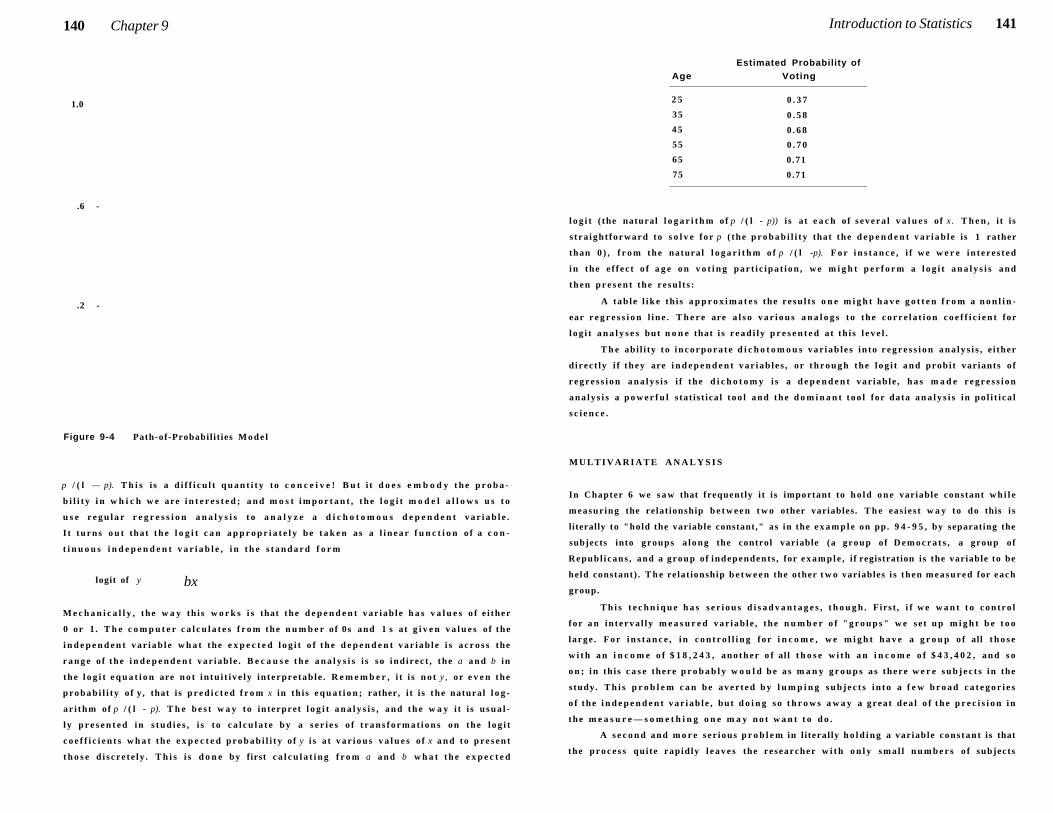
140 Chapter 9

1.0

.6 -

.2 -

Figure 9-4 Path-of-Probabil it ies M o d e l

p / ( l — p). T h i s i s a d i f f i c u l t q u a n t i t y to c o n c e i v e ! B u t i t d o e s e m b o d y t h e p r o b a ­

b i l i t y i n w h i c h w e are i n t e r e s t e d ; a n d m o s t i m p o r t a n t , t h e l o g i t m o d e l a l l o w s u s t o

u s e r e g u l a r r e g r e s s i o n a n a l y s i s t o a n a l y z e a d i c h o t o m o u s d e p e n d e n t v a r i a b l e .

I t t u r n s o u t that t h e l o g i t c a n a p p r o p r i a t e l y b e t a k e n a s a l i n e a r f u n c t i o n o f a c o n ­

t i n u o u s i n d e p e n d e n t v a r i a b l e , i n t h e s t a n d a r d f o r m

logit of y bx

M e c h a n i c a l l y , the w a y th i s w o r k s i s that the d e p e n d e n t var iab le h a s v a l u e s o f e i ther

0 or 1 . T h e c o m p u t e r c a l c u l a t e s f r o m the n u m b e r of 0s and 1 s a t g i v e n v a l u e s o f the

i n d e p e n d e n t v a r i a b l e w h a t the e x p e c t e d l o g i t o f t h e d e p e n d e n t v a r i a b l e i s a c r o s s the

r a n g e o f the i n d e p e n d e n t var iab le . B e c a u s e t h e a n a l y s i s i s so ind irec t , the a a n d b in

the l o g i t e q u a t i o n are n o t i n t u i t i v e l y in terpre tab le . R e m e m b e r , i t i s n o t y , or e v e n the

p r o b a b i l i t y o f y , that i s p r e d i c t e d f r o m x in th i s e q u a t i o n ; rather, i t i s t h e natural l o g ­

a r i t h m of p / ( l - p). T h e b e s t w a y to interpret l o g i t a n a l y s i s , a n d t h e w a y i t i s u s u a l ­

l y p r e s e n t e d i n s t u d i e s , i s t o c a l c u l a t e b y a s e r i e s o f t r a n s f o r m a t i o n s o n the l o g i t

c o e f f i c i e n t s w h a t the e x p e c t e d p r o b a b i l i t y o f y i s a t v a r i o u s v a l u e s o f x a n d to p r e s e n t

t h o s e d i s c r e t e l y . T h i s i s d o n e by first c a l c u l a t i n g f r o m a a n d b w h a t t h e e x p e c t e d

Introduction to Statistics 141

Estimated Probability of Age Voting

2 5 0 . 3 7

35 0 . 5 8

4 5 0 . 6 8

55 0 . 7 0

65 0 .71

75 0 .71

l o g i t ( the natural l o g a r i t h m of p / ( l - p)) i s at e a c h of s e v e r a l v a l u e s of x . T h e n , i t i s

s t ra ight forward to s o l v e for p ( the p r o b a b i l i t y that the d e p e n d e n t v a r i a b l e i s 1 rather

than 0 ) , f r o m the natural l o g a r i t h m o f p / ( l -p). F o r i n s t a n c e , i f w e w e r e i n t e r e s t e d

i n the e f f e c t o f a g e o n v o t i n g p a r t i c i p a t i o n , w e m i g h t p e r f o r m a l o g i t a n a l y s i s and

t h e n p r e s e n t the resu l t s :

A tab le l i k e th i s a p p r o x i m a t e s the re su l t s o n e m i g h t h a v e g o t t e n f r o m a n o n l i n ­

ear r e g r e s s i o n l i n e . T h e r e are a l s o v a r i o u s a n a l o g s t o the c o r r e l a t i o n c o e f f i c i e n t for

l o g i t a n a l y s e s but n o n e that i s r e a d i l y p r e s e n t e d a t th i s l e v e l .

T h e abi l i ty t o i n c o r p o r a t e d i c h o t o m o u s var iab le s in to r e g r e s s i o n a n a l y s i s , e i ther

d irec t ly i f t h e y are i n d e p e n d e n t v a r i a b l e s , or t h r o u g h the l o g i t a n d probi t variants o f

r e g r e s s i o n a n a l y s i s i f the d i c h o t o m y i s a d e p e n d e n t var iab le , h a s m a d e r e g r e s s i o n

a n a l y s i s a p o w e r f u l s tat i s t ica l t o o l and the d o m i n a n t t o o l for data a n a l y s i s in po l i t i ca l

s c i e n c e .

M U L T I V A R I A T E A N A L Y S I S

In Chapter 6 we s a w that frequently i t i s important to h o l d o n e variable constant w h i l e

measur ing the relat ionship b e t w e e n t w o other variables. T h e eas ies t w a y to do this i s

literally to "hold the variable constant," as in the e x a m p l e on pp. 9 4 - 9 5 , by separating the

subjects into groups a l o n g the control variable (a group of D e m o c r a t s , a group of

Republ i cans , and a group of independents , for e x a m p l e , i f registration is the variable to be

he ld constant) . T h e relat ionship b e t w e e n the other t w o variables i s then m e a s u r e d for each

group.

T h i s t e c h n i q u e h a s s e r i o u s d i s a d v a n t a g e s , t h o u g h . First , i f w e w a n t t o c o n t r o l

for a n in t erva l l y m e a s u r e d var iab le , the n u m b e r o f " g r o u p s " w e se t u p m i g h t b e t o o

large . F o r i n s t a n c e , i n c o n t r o l l i n g for i n c o m e , w e m i g h t h a v e a g r o u p o f all t h o s e

w i t h a n i n c o m e o f $ 1 8 , 2 4 3 , a n o t h e r o f al l t h o s e w i t h a n i n c o m e o f $ 4 3 , 4 0 2 , a n d s o

o n ; i n th i s c a s e there p r o b a b l y w o u l d b e a s m a n y g r o u p s a s there w e r e s u b j e c t s i n the

s tudy. T h i s p r o b l e m c a n b e a v e r t e d b y l u m p i n g s u b j e c t s i n t o a f e w b r o a d c a t e g o r i e s

o f the i n d e p e n d e n t v a r i a b l e , but d o i n g s o t h r o w s a w a y a great d e a l o f t h e p r e c i s i o n i n

the m e a s u r e — s o m e t h i n g o n e m a y n o t w a n t t o d o .

A s e c o n d and m o r e ser ious p r o b l e m in l i teral ly h o l d i n g a var iable cons tant is that

the p r o c e s s qui te rapid ly l e a v e s the researcher w i t h o n l y s m a l l n u m b e r s o f subjects

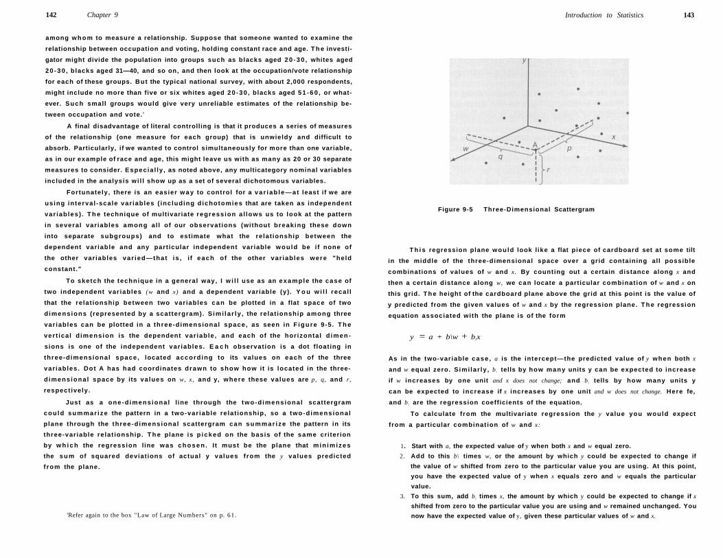
142 Chapter 9

among whom to measure a relationship. Suppose that someone wanted to examine the

relationship between occupation and voting, holding constant race and age. T h e investi­

gator might divide the population into groups such as blacks aged 2 0 - 3 0 , whites aged

2 0 - 3 0 , blacks aged 31—40, and so on, and then look at the occupation/vote relationship

for each of these groups. But the typical national survey, with about 2,000 respondents,

might include no more than five or six whites aged 2 0 - 3 0 , blacks aged 5 1 - 6 0 , or what­

ever. Such small groups would give very unreliable estimates of the relationship be­

tween occupation and vote. 5

A final disadvantage of literal controlling is that it produces a series of measures

of the relationship (one measure for each group) that is unwieldy and difficult to

absorb. Particularly, if we wanted to control simultaneously for more than one variable,

as in our example of race and age, this might leave us with as many as 20 or 30 separate

measures to consider. Especia l ly , as noted above, any multicategory nominal variables

included in the analysis wi l l show up as a set of several dichotomous variables.

Fortunately, there is an easier w a y to control for a va r iab le—at least if we are

using interval -scale var iables ( including d ichotomies that are taken as independent

var iab les) . T h e technique of multivariate regression a l lows us to look at the pattern

in several var iables among al l of our observat ions (without breaking these down

into separate subgroups) and to estimate what the relat ionship between the

dependent var iable and any part icular independent variable wou ld be i f none of

the other variables var ied—that is , i f each of the other var iables were "held

constant."

To sketch the technique in a general way, I w i l l use as an example the case of

two independent var iables (w and x) and a dependent variable (y) . Y o u w i l l recal l

that the relat ionship between two variables can be plotted in a flat space of two

d imensions (represented by a scattergram). S imi la r ly , the relat ionship among three

var iables can be plotted in a three-dimensional space, as seen in F igure 9-5. T h e

vert ica l d imension is the dependent var iable , and each of the horizontal d imen­

sions is one of the independent var iables. E a c h observation is a dot f loating in

three-dimensional space, located accord ing to its values on each of the three

var iables. Dot A has had coordinates drawn to show how it is located in the three-

d imensiona l space by its values on w, x, and y, where these values are p, q, and r,

respectively.

Just as a one-d imensiona l l ine through the two-d imensional scattergram

cou ld summar ize the pattern in a two-var iable relat ionship, so a two-d imensional

plane through the three-d imensional scattergram can summar ize the pattern in its

three-variable relat ionship. T h e plane is p icked on the basis of the same criterion

by w h i c h the regression line was c h o s e n . I t must be the plane that m in imizes

the sum of squared deviat ions of actual y values f rom the y va lues predicted

f rom the plane.

'Refer again to the box "Law of Large Numbers" on p. 61.

Introduction to Statistics 143

Figure 9-5 Three-Dimensional Scattergram

T h i s regression plane would look l ike a flat piece of cardboard set at some tilt

in the middle of the three-dimensional space over a grid containing all possible

combinations of values of w and x. By counting out a certain distance along x and

then a certain distance along w, we can locate a particular combinat ion of w and x on

this grid. T h e height of the cardboard plane above the grid at this point is the value of

y predicted from the given values of w and x by the regression plane. T h e regression

equation associated with the plane is of the form

y = a + b\w + b2x

As in the two-variable case , a is the intercept—the predicted value of y when both x

and w equal zero. S imi lar ly , b x tells by how many units y can be expected to increase

if w increases by one unit and x does not change; and b 2 tells by how many units y

can be expected to increase if x increases by one unit and w does not change. Here fe,

and b 2 are the regression coefficients of the equation.

To calculate f rom the multivariate regression the y value you would expect

from a particular combinat ion of w and x:

1. Start with a, the expected value of y when both x and w equal zero.

2. Add to this b\ times w, or the amount by which y could be expected to change if

the value of w shifted from zero to the particular value you are using. At this point,

you have the expected value of y when x equals zero and w equals the particular

value.

3. To this sum, add b2 times x, the amount by which y could be expected to change if x

shifted from zero to the particular value you are using and w remained unchanged. You

now have the expected value of y, given these particular values of w and x.

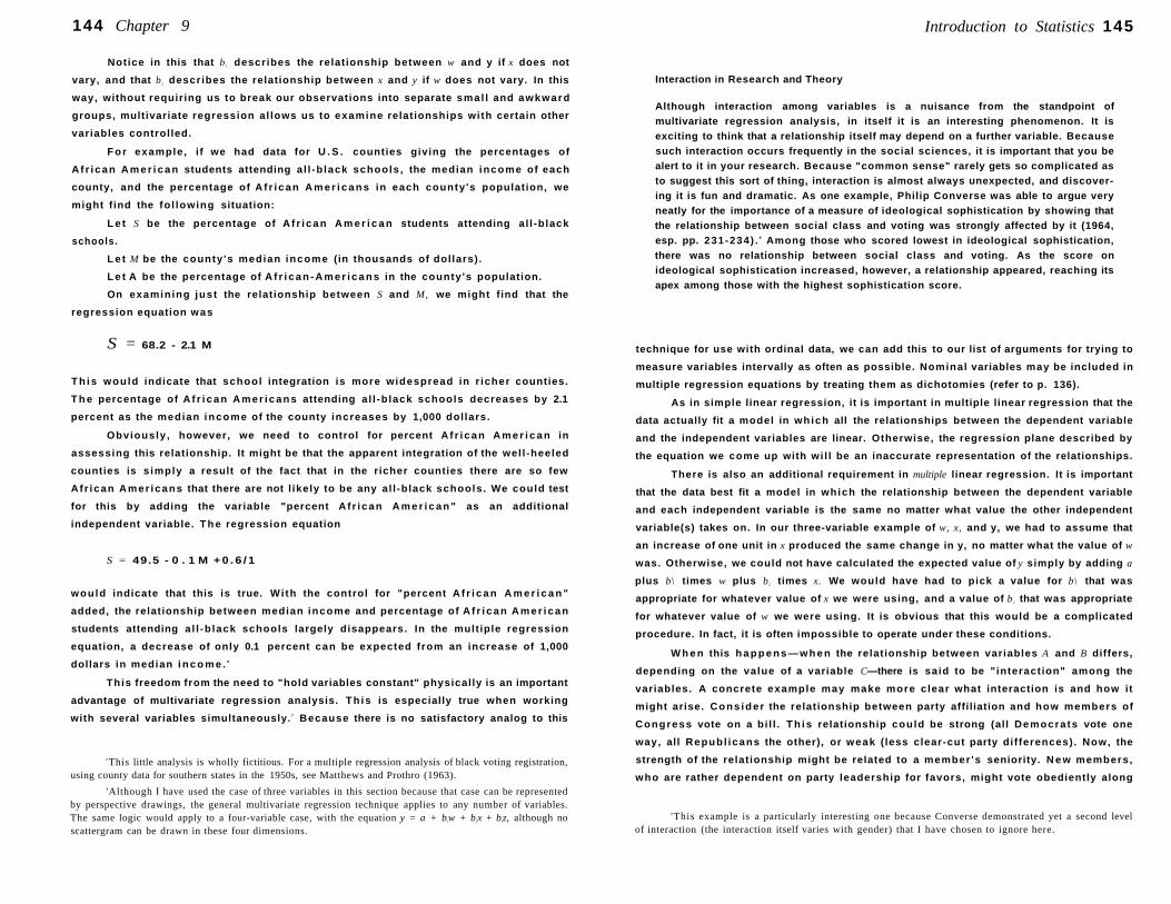
144 Chapter 9

Notice in this that b { describes the relationship between w and y if x does not

vary, and that b 2 describes the relationship between x and y if w does not vary. In this

way, without requiring us to break our observations into separate smal l and awkward

groups, multivariate regression al lows us to examine relationships with certain other

variables controlled.

F o r example, i f we had data for U . S . counties giving the percentages of

A f r i can A m e r i c a n students attending a l l -b lack schools , the median income of each

county, and the percentage of A f r i can A m e r i c a n s in each county's population, we

might f ind the fo l lowing situation:

L e t S be the percentage of A f r i can A m e r i c a n students attending al l -black

schools.

L e t M be the county 's median income (in thousands of dollars) .

L e t A be the percentage of A f r i c a n - A m e r i c a n s in the county's population.

On examining just the relationship between S and M, we might find that the

regression equation was

S = 68.2 - 2.1 M

T h i s would indicate that school integration is more widespread in r icher counties.

T h e percentage of A f r i c a n A m e r i c a n s attending al l -b lack schools decreases by 2.1

percent as the median income of the county increases by 1,000 dollars.

Obviously , however, we need to control for percent A f r i can A m e r i c a n in

assessing this relationship. It might be that the apparent integration of the wel l -heeled

counties is s imply a result of the fact that in the richer counties there are so few

Af r ican Amer icans that there are not l ikely to be any al l -black schools. We could test

for this by adding the variable "percent A f r ican A m e r i c a n " as an additional

independent variable. T h e regression equation

S = 49.5 - 0 . 1 M + 0 . 6 / 1

would indicate that this is true. Wi th the control for "percent A f r i c a n A m e r i c a n "

added, the relationship between median income and percentage of A f r i c a n A m e r i c a n

students attending a l l -b lack schools largely disappears. In the mult iple regression

equation, a decrease of only 0.1 percent can be expected from an increase of 1,000

dollars in median i n c o m e . 6

This freedom from the need to "hold variables constant" physically is an important

advantage of multivariate regression analysis. Th is is especially true when working

with several variables simultaneously. 7 Because there is no satisfactory analog to this

6This little analysis is wholly fictitious. For a multiple regression analysis of black voting registration, using county data for southern states in the 1950s, see Matthews and Prothro (1963).

'Although I have used the case of three variables in this section because that case can be represented by perspective drawings, the general multivariate regression technique applies to any number of variables. The same logic would apply to a four-variable case, with the equation y = a + b{w + b2x + b}z, although no scattergram can be drawn in these four dimensions.

Introduction to Statistics 145

Interaction in Research and Theory

Although interaction among variables is a nuisance from the standpoint of multivariate regression analysis, in itself it is an interesting phenomenon. It is exciting to think that a relationship itself may depend on a further variable. Because such interaction occurs frequently in the social sciences, it is important that you be alert to it in your research. Because "common sense" rarely gets so complicated as to suggest this sort of thing, interaction is almost always unexpected, and discover­ing it is fun and dramatic. As one example, Philip Converse was able to argue very neatly for the importance of a measure of ideological sophistication by showing that the relationship between social class and voting was strongly affected by it (1964, esp. pp. 231-234) . 8 Among those who scored lowest in ideological sophistication, there was no relationship between social class and voting. As the score on ideological sophistication increased, however, a relationship appeared, reaching its apex among those with the highest sophistication score.

technique for use with ordinal data, we can add this to our list of arguments for trying to

measure variables intervally as often as possible. Nominal variables may be included in

multiple regression equations by treating them as dichotomies (refer to p. 136).

As in simple linear regression, it is important in multiple linear regression that the

data actually fit a model in which all the relationships between the dependent variable

and the independent variables are linear. Otherwise, the regression plane described by

the equation we come up with wi l l be an inaccurate representation of the relationships.

There is also an additional requirement in multiple linear regression. It is important

that the data best fit a model in which the relationship between the dependent variable

and each independent variable is the same no matter what value the other independent

variable(s) takes on. In our three-variable example of w, x, and y, we had to assume that

an increase of one unit in x produced the same change in y, no matter what the value of w

was. Otherwise, we could not have calculated the expected value of y simply by adding a

plus b\ times w plus b 2 times x. We would have had to pick a value for b\ that was

appropriate for whatever value of x we were using, and a value of b 2 that was appropriate

for whatever value of w we were using. It is obvious that this would be a complicated

procedure. In fact, it is often impossible to operate under these conditions.

W h e n this h a p p e n s — w h e n the relationship between variables A and B differs,

depending on the value of a variable C—there is said to be "interaction" among the

variables. A concrete example may make more clear what interaction is and how it

might arise. Cons ider the relationship between party affiliation and how members of

Congress vote on a bi l l . T h i s relationship could be strong (all Democrats vote one

way, all Republ icans the other), or weak ( less clear-cut party dif ferences). Now, the

strength of the relationship might be related to a member 's seniority. N e w members,

who are rather dependent on party leadership for favors, might vote obediently along

8 This example is a particularly interesting one because Converse demonstrated yet a second level of interaction (the interaction itself varies with gender) that I have chosen to ignore here.

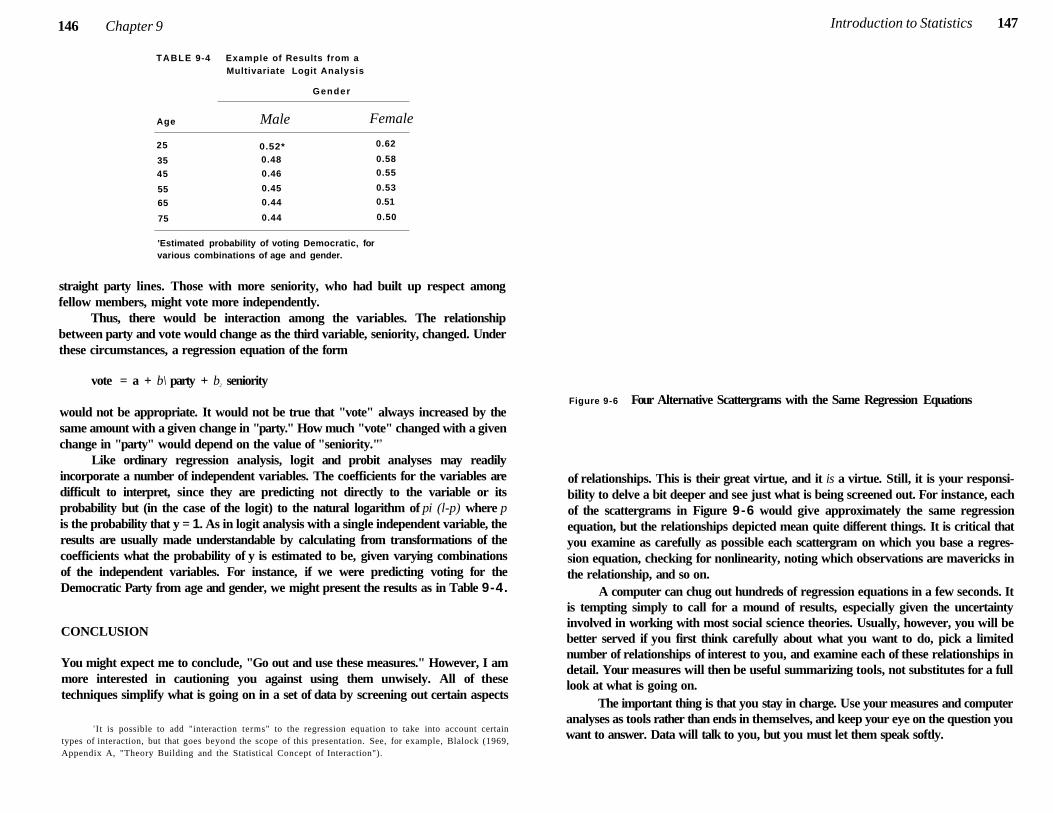
146 Chapter 9

TABLE 9-4 Example of Results from a Multivariate Logit Analysis

Gender

Age Male Female

25 0.52* 0.62

35 0.48 0.58

45 0.46 0.55

55 0.45 0.53

65 0.44 0.51

75 0.44 0.50

'Estimated probability of voting Democratic, for various combinations of age and gender.

straight party lines. Those with more seniority, who had built up respect among fellow members, might vote more independently.

Thus, there would be interaction among the variables. The relationship between party and vote would change as the third variable, seniority, changed. Under these circumstances, a regression equation of the form

vote = a + b\ party + b2 seniority

would not be appropriate. It would not be true that "vote" always increased by the same amount with a given change in "party." How much "vote" changed with a given change in "party" would depend on the value of "seniority."9

Like ordinary regression analysis, logit and probit analyses may readily incorporate a number of independent variables. The coefficients for the variables are difficult to interpret, since they are predicting not directly to the variable or its probability but (in the case of the logit) to the natural logarithm of pi (l-p) where p is the probability that y = 1. As in logit analysis with a single independent variable, the results are usually made understandable by calculating from transformations of the coefficients what the probability of y is estimated to be, given varying combinations of the independent variables. For instance, if we were predicting voting for the Democratic Party from age and gender, we might present the results as in Table 9-4.

CONCLUSION

You might expect me to conclude, "Go out and use these measures." However, I am more interested in cautioning you against using them unwisely. All of these techniques simplify what is going on in a set of data by screening out certain aspects

9 It is possible to add "interaction terms" to the regression equation to take into account certain types of interaction, but that goes beyond the scope of this presentation. See, for example, Blalock (1969, Appendix A, "Theory Building and the Statistical Concept of Interaction").

Introduction to Statistics 147

Figure 9-6 Four Alternative Scattergrams with the Same Regression Equations

of relationships. This is their great virtue, and it is a virtue. Still, it is your responsi­bility to delve a bit deeper and see just what is being screened out. For instance, each of the scattergrams in Figure 9-6 would give approximately the same regression equation, but the relationships depicted mean quite different things. It is critical that you examine as carefully as possible each scattergram on which you base a regres­sion equation, checking for nonlinearity, noting which observations are mavericks in the relationship, and so on.

A computer can chug out hundreds of regression equations in a few seconds. It is tempting simply to call for a mound of results, especially given the uncertainty involved in working with most social science theories. Usually, however, you will be better served if you first think carefully about what you want to do, pick a limited number of relationships of interest to you, and examine each of these relationships in detail. Your measures will then be useful summarizing tools, not substitutes for a full look at what is going on.

The important thing is that you stay in charge. Use your measures and computer analyses as tools rather than ends in themselves, and keep your eye on the question you want to answer. Data will talk to you, but you must let them speak softly.

Chapter 10

Inference, or How to Gamble on Your Research

As I pointed out in Chapte r 8, there are two m a i n areas of stat ist ics: (1) measur ing

things, espec ia l ly measur ing relat ionships between var iab les; and (2) est imat ing

how l ike ly i t is that the measure you have gotten cou ld have occur red by chance .

In Chapters 8 and 9 we looked at the first of these aspects , and now we examine

the second . (I must note parenthet ical ly that, as in preceding chapters , I do not

intend to teach y o u how to use stat ist ical tests. Instead I present the general logic

of such tests to help y o u understand what they m e a n w h e n you see them. T h i s

approach might a lso serve as a useful supplement to a statist ics course , w h i c h

somet imes teaches students how to use the tests without putting the tests in a

broader perspect ive. )

It is quite possible to get a particular result by chance, even though the result is

not true in general. If you chose ten U . S . senators at random, for instance, it would

be possible to come up with a group consist ing largely of conservative Democrats

and l iberal Republ icans . F r o m that you might conc lude—erroneous ly—that there

was a relationship between party and ideology in the Senate, with Republ icans the

more l iberal group.

However, if you repeatedly drew groups of ten senators, selecting the ten at

random from the whole Senate, most of the time you would find that the Democrats in

your group were more liberal than the Republ icans, simply because Democratic

senators do tend to be more liberal than Republ ican senators. But some of the time you

would find that the Republ icans in your sample were more liberal than the Democrats,

or that the two parties did not differ at all . T h e problem in drawing a single group and

describing the Senate from it is that you cannot know whether your group is of the first

type (the relationship between the variables is the same in your subset as in the Senate

as a whole) or of the second (the relationship between the variables is different in the

148

Introduction to Statistics 149

subset from that in the Senate as a whole) . If it is of the first type, your conclusion wil l

be true; if it is of the second (a distorted sample) , your conclusion wi l l be false. T h i s is

a common problem that must be dealt with whenever anyone tries to describe a whole

population of cases by looking only at a sample drawn out of the population. It comes

up in conducting social science research, opinion polling, assigning television ratings,

conducting market analyses, administering quality control in manufacturing, and in

performing numerous other activities.

Fortunately, there are w a y s to determine just how l ikely it is that a particular

result could have occurred by chance even i f its opposite were generally true. By

means of these techniques we can calculate how much stock to put in our f indings. It

is a very close analogy to say that we can gamble intelligently on the results of our

study by calculat ing the odds that the results are false. W h e n we do this, we are said

to measure (or "test") the statistical significance of our results.

In looking at how to measure relationships in Chapter 9, we found that there

were qualitatively different ways to go about it, depending on the level at w h i c h the

variables were measured. In measur ing the statistical s ignif icance of a relationship,

one broad procedure holds for all levels of data, although there are differences in

specif ic techniques.

L O G I C O F M E A S U R I N G S I G N I F I C A N C E

T h e general procedure by w h i c h we calculate t i e probability that a given result could

have occurred by chance, even though the true state of affairs was something other

than what is indicated by the result, is the same procedure that we use in calculating

the odds of any event happening.

As usual when talking about probability, let us start with a deck of cards. G iven

an honest deck of cards, thoroughly shuffled, you are instructed to draw a card. Y o u

know that the probability that you wi l l draw the king of hearts is 1/52, for there are 52

cards and only one of them is the king of hearts. Next, you are instructed to do this

two times, replacing the card and reshuffling after the first draw. Y o u know that the

probability of drawing a king of hearts both times is 1/52 x 1/52 = 1/2704, or 0.00037,

and so o n . 1

You were able to calculate these probabilities because, given a sufficient set

of assumptions, the probability that any particular result would occur could be

determined. These assumptions had to account for al l of the factors that could

influence the outcome of the drawing. With such a set of assumptions, it was possible

'The logic of this is as follows: In order to draw two kings of hearts in two draws, you must accomplish two things. First, you must draw the king of hearts on the first round. This can be expected to happen only one fifty-second of the time. Now, assuming that you have succeeded in the first round, you still can expect success in the second round only one fifty-second of the time. In other words, in the full two-draw process, you can expect to proceed to final success only one fifty-second of one fifty-second of the time.

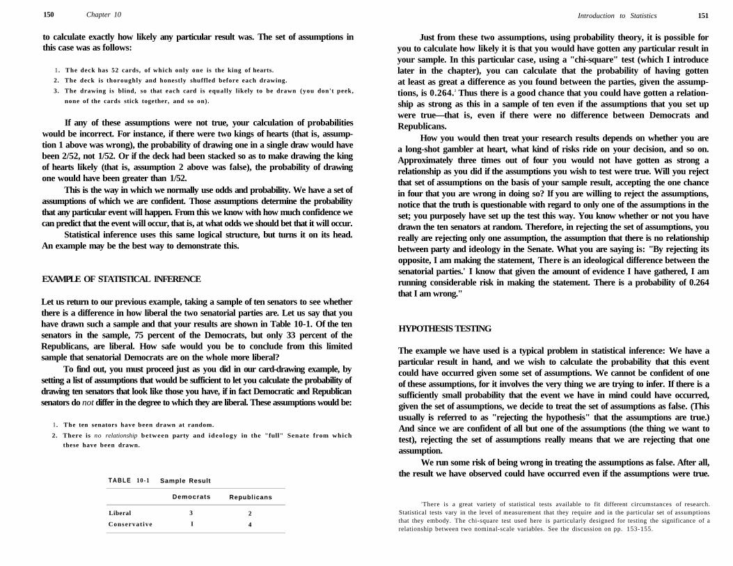
150 Chapter 10

to calculate exactly how likely any particular result was. The set of assumptions in this case was as follows:

1 . The deck has 52 cards, of which only one is the king of hearts.

2. The deck is thoroughly and honestly shuffled before each drawing.

3. The drawing is blind, so that each card is equally likely to be drawn (you don't peek,

none of the cards stick together, and so on).

If any of these assumptions were not true, your calculation of probabilities would be incorrect. For instance, if there were two kings of hearts (that is, assump­tion 1 above was wrong), the probability of drawing one in a single draw would have been 2/52, not 1/52. Or if the deck had been stacked so as to make drawing the king of hearts likely (that is, assumption 2 above was false), the probability of drawing one would have been greater than 1/52.

This is the way in which we normally use odds and probability. We have a set of assumptions of which we are confident. Those assumptions determine the probability that any particular event will happen. From this we know with how much confidence we can predict that the event will occur, that is, at what odds we should bet that it will occur.

Statistical inference uses this same logical structure, but turns it on its head. An example may be the best way to demonstrate this.

EXAMPLE OF STATISTICAL INFERENCE

Let us return to our previous example, taking a sample of ten senators to see whether there is a difference in how liberal the two senatorial parties are. Let us say that you have drawn such a sample and that your results are shown in Table 10-1. Of the ten senators in the sample, 75 percent of the Democrats, but only 33 percent of the Republicans, are liberal. How safe would you be to conclude from this limited sample that senatorial Democrats are on the whole more liberal?

To find out, you must proceed just as you did in our card-drawing example, by setting a list of assumptions that would be sufficient to let you calculate the probability of drawing ten senators that look like those you have, if in fact Democratic and Republican senators do not differ in the degree to which they are liberal. These assumptions would be:

1. The ten senators have been drawn at random.

2. There is no relationship between party and ideology in the "full" Senate from which

these have been drawn.

TABLE 10 -1 Sample Result

Democrats Republicans

Liberal 3 2

Conservat ive I 4

Introduction to Statistics 151

Just from these two assumptions, using probability theory, it is possible for you to calculate how likely it is that you would have gotten any particular result in your sample. In this particular case, using a "chi-square" test (which I introduce later in the chapter), you can calculate that the probability of having gotten at least as great a difference as you found between the parties, given the assump­tions, is 0.264.2 Thus there is a good chance that you could have gotten a relation­ship as strong as this in a sample of ten even if the assumptions that you set up were true—that is, even if there were no difference between Democrats and Republicans.

How you would then treat your research results depends on whether you are a long-shot gambler at heart, what kind of risks ride on your decision, and so on. Approximately three times out of four you would not have gotten as strong a relationship as you did if the assumptions you wish to test were true. Will you reject that set of assumptions on the basis of your sample result, accepting the one chance in four that you are wrong in doing so? If you are willing to reject the assumptions, notice that the truth is questionable with regard to only one of the assumptions in the set; you purposely have set up the test this way. You know whether or not you have drawn the ten senators at random. Therefore, in rejecting the set of assumptions, you really are rejecting only one assumption, the assumption that there is no relationship between party and ideology in the Senate. What you are saying is: "By rejecting its opposite, I am making the statement, There is an ideological difference between the senatorial parties.' I know that given the amount of evidence I have gathered, I am running considerable risk in making the statement. There is a probability of 0.264 that I am wrong."

HYPOTHESIS TESTING

The example we have used is a typical problem in statistical inference: We have a particular result in hand, and we wish to calculate the probability that this event could have occurred given some set of assumptions. We cannot be confident of one of these assumptions, for it involves the very thing we are trying to infer. If there is a sufficiently small probability that the event we have in mind could have occurred, given the set of assumptions, we decide to treat the set of assumptions as false. (This usually is referred to as "rejecting the hypothesis" that the assumptions are true.) And since we are confident of all but one of the assumptions (the thing we want to test), rejecting the set of assumptions really means that we are rejecting that one assumption.

We run some risk of being wrong in treating the assumptions as false. After all, the result we have observed could have occurred even if the assumptions were true.

2 There is a great variety of statistical tests available to fit different circumstances of research. Statistical tests vary in the level of measurement that they require and in the particular set of assumptions that they embody. The chi-square test used here is particularly designed for testing the significance of a relationship between two nominal-scale variables. See the discussion on pp. 153-155.

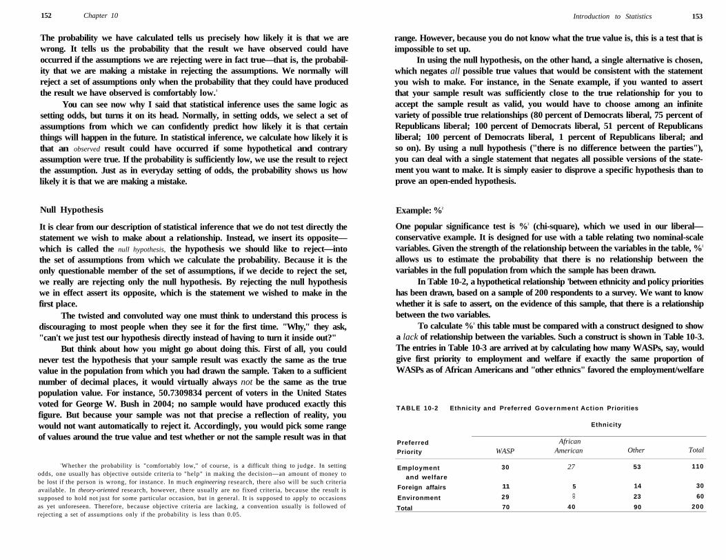
152 Chapter 10

The probability we have calculated tells us precisely how likely it is that we are wrong. It tells us the probability that the result we have observed could have occurred if the assumptions we are rejecting were in fact true—that is, the probabil­ity that we are making a mistake in rejecting the assumptions. We normally will reject a set of assumptions only when the probability that they could have produced the result we have observed is comfortably low.3

You can see now why I said that statistical inference uses the same logic as setting odds, but turns it on its head. Normally, in setting odds, we select a set of assumptions from which we can confidently predict how likely it is that certain things will happen in the future. In statistical inference, we calculate how likely it is that an observed result could have occurred if some hypothetical and contrary assumption were true. If the probability is sufficiently low, we use the result to reject the assumption. Just as in everyday setting of odds, the probability shows us how likely it is that we are making a mistake.

Null Hypothesis

It is clear from our description of statistical inference that we do not test directly the statement we wish to make about a relationship. Instead, we insert its opposite— which is called the null hypothesis, the hypothesis we should like to reject—into the set of assumptions from which we calculate the probability. Because it is the only questionable member of the set of assumptions, if we decide to reject the set, we really are rejecting only the null hypothesis. By rejecting the null hypothesis we in effect assert its opposite, which is the statement we wished to make in the first place.

The twisted and convoluted way one must think to understand this process is discouraging to most people when they see it for the first time. "Why," they ask, "can't we just test our hypothesis directly instead of having to turn it inside out?"

But think about how you might go about doing this. First of all, you could never test the hypothesis that your sample result was exactly the same as the true value in the population from which you had drawn the sample. Taken to a sufficient number of decimal places, it would virtually always not be the same as the true population value. For instance, 50.7309834 percent of voters in the United States voted for George W. Bush in 2004; no sample would have produced exactly this figure. But because your sample was not that precise a reflection of reality, you would not want automatically to reject it. Accordingly, you would pick some range of values around the true value and test whether or not the sample result was in that

3 Whether the probability is "comfortably low," of course, is a difficult thing to judge. In setting odds, one usually has objective outside criteria to "help" in making the decision—an amount of money to be lost if the person is wrong, for instance. In much engineering research, there also will be such criteria available. In theory-oriented research, however, there usually are no fixed criteria, because the result is supposed to hold not just for some particular occasion, but in general. It is supposed to apply to occasions as yet unforeseen. Therefore, because objective criteria are lacking, a convention usually is followed of rejecting a set of assumptions only if the probability is less than 0.05.

Introduction to Statistics 153

range. However, because you do not know what the true value is, this is a test that is impossible to set up.

In using the null hypothesis, on the other hand, a single alternative is chosen, which negates all possible true values that would be consistent with the statement you wish to make. For instance, in the Senate example, if you wanted to assert that your sample result was sufficiently close to the true relationship for you to accept the sample result as valid, you would have to choose among an infinite variety of possible true relationships (80 percent of Democrats liberal, 75 percent of Republicans liberal; 100 percent of Democrats liberal, 51 percent of Republicans liberal; 100 percent of Democrats liberal, 1 percent of Republicans liberal; and so on). By using a null hypothesis ("there is no difference between the parties"), you can deal with a single statement that negates all possible versions of the state­ment you want to make. It is simply easier to disprove a specific hypothesis than to prove an open-ended hypothesis.

Example: %2

One popular significance test is %2 (chi-square), which we used in our liberal— conservative example. It is designed for use with a table relating two nominal-scale variables. Given the strength of the relationship between the variables in the table, %2

allows us to estimate the probability that there is no relationship between the variables in the full population from which the sample has been drawn.

In Table 10-2, a hypothetical relationship 'between ethnicity and policy priorities has been drawn, based on a sample of 200 respondents to a survey. We want to know whether it is safe to assert, on the evidence of this sample, that there is a relationship between the two variables.

To calculate %2 this table must be compared with a construct designed to show a lack of relationship between the variables. Such a construct is shown in Table 10-3. The entries in Table 10-3 are arrived at by calculating how many WASPs, say, would give first priority to employment and welfare if exactly the same proportion of WASPs as of African Americans and "other ethnics" favored the employment/welfare

TABLE 10-2 Ethnicity and Preferred Government Action Priorities

Ethnicity

Preferred Priority WASP

African American Other Total

Employment 30 27 53 110

and welfare

Foreign affairs 11 5 14 30

Environment 29

CO

23 60

Total 70 40 90 200

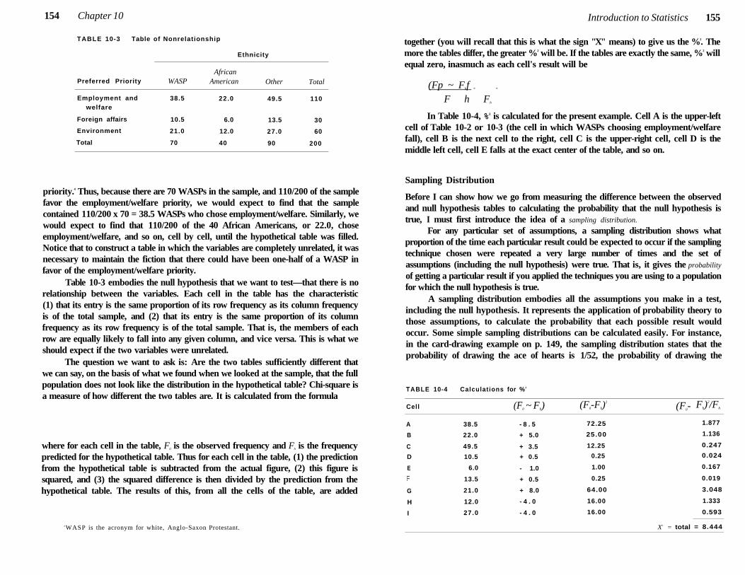
154 Chapter 10

Ethnicity

Preferred Priority WASP African

American Other Total

Employment and welfare

38.5 22.0 49.5 110

Foreign affairs 10.5 6.0 13.5 30

Environment 21.0 12.0 27.0 60

Total 70 40 90 200

priority.4 Thus, because there are 70 WASPs in the sample, and 110/200 of the sample favor the employment/welfare priority, we would expect to find that the sample contained 110/200 x 70 = 38.5 WASPs who chose employment/welfare. Similarly, we would expect to find that 110/200 of the 40 African Americans, or 22.0, chose employment/welfare, and so on, cell by cell, until the hypothetical table was filled. Notice that to construct a table in which the variables are completely unrelated, it was necessary to maintain the fiction that there could have been one-half of a WASP in favor of the employment/welfare priority.

Table 10-3 embodies the null hypothesis that we want to test—that there is no relationship between the variables. Each cell in the table has the characteristic (1) that its entry is the same proportion of its row frequency as its column frequency is of the total sample, and (2) that its entry is the same proportion of its column frequency as its row frequency is of the total sample. That is, the members of each row are equally likely to fall into any given column, and vice versa. This is what we should expect if the two variables were unrelated.

The question we want to ask is: Are the two tables sufficiently different that we can say, on the basis of what we found when we looked at the sample, that the full population does not look like the distribution in the hypothetical table? Chi-square is a measure of how different the two tables are. It is calculated from the formula

where for each cell in the table, F0 is the observed frequency and Fh is the frequency predicted for the hypothetical table. Thus for each cell in the table, (1) the prediction from the hypothetical table is subtracted from the actual figure, (2) this figure is squared, and (3) the squared difference is then divided by the prediction from the hypothetical table. The results of this, from all the cells of the table, are added

4 WASP is the acronym for white, Anglo-Saxon Protestant.

Introduction to Statistics 155

together (you will recall that this is what the sign "X" means) to give us the %2. The more the tables differ, the greater %2 will be. If the tables are exactly the same, %2 will equal zero, inasmuch as each cell's result will be

(Fp ~ Fhf = =

F h Fh

In Table 10-4, %2 is calculated for the present example. Cell A is the upper-left cell of Table 10-2 or 10-3 (the cell in which WASPs choosing employment/welfare fall), cell B is the next cell to the right, cell C is the upper-right cell, cell D is the middle left cell, cell E falls at the exact center of the table, and so on.

Sampling Distribution

Before I can show how we go from measuring the difference between the observed and null hypothesis tables to calculating the probability that the null hypothesis is true, I must first introduce the idea of a sampling distribution.

For any particular set of assumptions, a sampling distribution shows what proportion of the time each particular result could be expected to occur if the sampling technique chosen were repeated a very large number of times and the set of assumptions (including the null hypothesis) were true. That is, it gives the probability

of getting a particular result if you applied the techniques you are using to a population for which the null hypothesis is true.

A sampling distribution embodies all the assumptions you make in a test, including the null hypothesis. It represents the application of probability theory to those assumptions, to calculate the probability that each possible result would occur. Some simple sampling distributions can be calculated easily. For instance, in the card-drawing example on p. 149, the sampling distribution states that the probability of drawing the ace of hearts is 1/52, the probability of drawing the

TABLE 10-4 Calculat ions for % 2

Cell (F0 ~ Fh) (F0-Fh)2

(F0- Fh)2/Fh

A 38.5 - 8 . 5 72.25 1.877

B 22.0 + 5.0 25.00 1.136

C 49.5 + 3.5 12.25 0.247

D 10.5 + 0.5 0.25 0.024

E 6.0 - 1.0 1.00 0.167

LL

. 13.5 + 0.5 0.25 0.019

G 21.0 + 8.0 64.00 3.048

H 12.0 - 4 . 0 16.00 1.333

I 27.0 - 4 . 0 16.00 0.593

X2 = total = 8.444

TABLE 10-3 Table of Nonrelationship

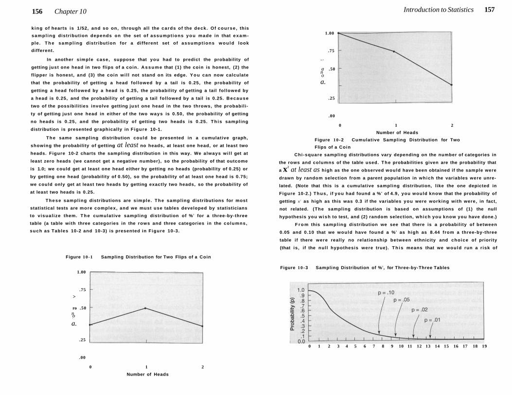
156 Chapter 10

k ing of hearts is 1/52, and so on, through al l the cards of the deck . Of course , this

sampl ing distr ibution depends on the set of assumpt ions y o u made in that e x a m ­

ple. T h e sampl ing distr ibution for a different set of assumpt ions w o u l d look

different.

In another simple case, suppose that you had to predict the probability of

getting just one head in two flips of a coin. A s s u m e that (1) the coin is honest, (2) the

flipper is honest, and (3) the coin w i l l not stand on its edge. Y o u can now calculate

that the probability of getting a head fol lowed by a tail is 0.25, the probability of

getting a head fol lowed by a head is 0.25, the probability of getting a tail fol lowed by

a head is 0.25, and the probability of getting a tail fol lowed by a tail is 0.25. B e c a u s e

two of the possibil it ies involve getting just one head in the two throws, the probabil i­

ty of getting just one head in either of the two ways is 0.50, the probability of getting

no heads is 0.25, and the probability of getting two heads is 0.25. T h i s sampling

distribution is presented graphically in F igure 10-1.

T h e same sampling distribution could be presented in a cumulative graph,

showing the probability of getting at least no heads, at least one head, or at least two

heads. Figure 10-2 charts the sampling distribution in this way. We always wi l l get at

least zero heads (we cannot get a negative number), so the probability of that outcome

is 1.0; we could get at least one head either by getting no heads (probability of 0.25) or

by getting one head (probability of 0.50), so the probability of at least one head is 0.75;

we could only get at least two heads by getting exactly two heads, so the probability of

at least two heads is 0.25.

T h e s e sampl ing distributions are simple. T h e sampling distributions for most

statistical tests are more complex, and we must use tables developed by statisticians

to v isual ize them. T h e cumulat ive sampling distribution of % 2 for a three-by-three

table (a table with three categories in the rows and three categories in the co lumns,

such as Tables 10-2 and 10-3) is presented in F igure 10-3.

Figure 10 -1 Sampling Distribution for Two Flips of a Coin

1.00

.75

>

ro .50 n o

i _

a.

.25

.00

0 1 2

Number of Heads

Introduction to Statistics 157

1.00

.75

+ ^

a .50 n o a.

.25

.00

0 1 2

Number of Heads

Figure 1 0 - 2 Cumulative Sampling Distribution for Two

Flips of a Coin

Chi-square sampling distributions vary depending on the number of categories in

the rows and columns of the table used. T h e probabilities given are the probability that

a x2 at least as high as the one observed would have been obtained if the sample were

drawn by random selection from a parent population in which the variables were unre­

lated. (Note that this is a cumulative sampling distribution, like the one depicted in

Figure 10-2.) Thus , if you had found a % 2 of 4.9, you would know that the probability of

getting x 2 as high as this was 0.3 if the variables you were working with were, in fact,

not related. (The sampling distribution is based on assumptions of (1) the null

hypothesis you w i s h to test, and (2) random selection, which you know you have done.)

F r o m this sampl ing distribution we see that there is a probability of between

0.05 and 0.10 that we would have found a % 2 as high as 8.44 from a three-by-three

table if there were really no relationship between ethnicity and choice of priority

(that is , if the nul l hypothesis were true). T h i s means that we would run a r isk of

Figure 1 0 - 3 Sampling Distribution of % 2, for Three-by-Three Tables

0 1 2 3 4 5 6 7 8 9 10 11 12 13 14 15 16 17 18 19

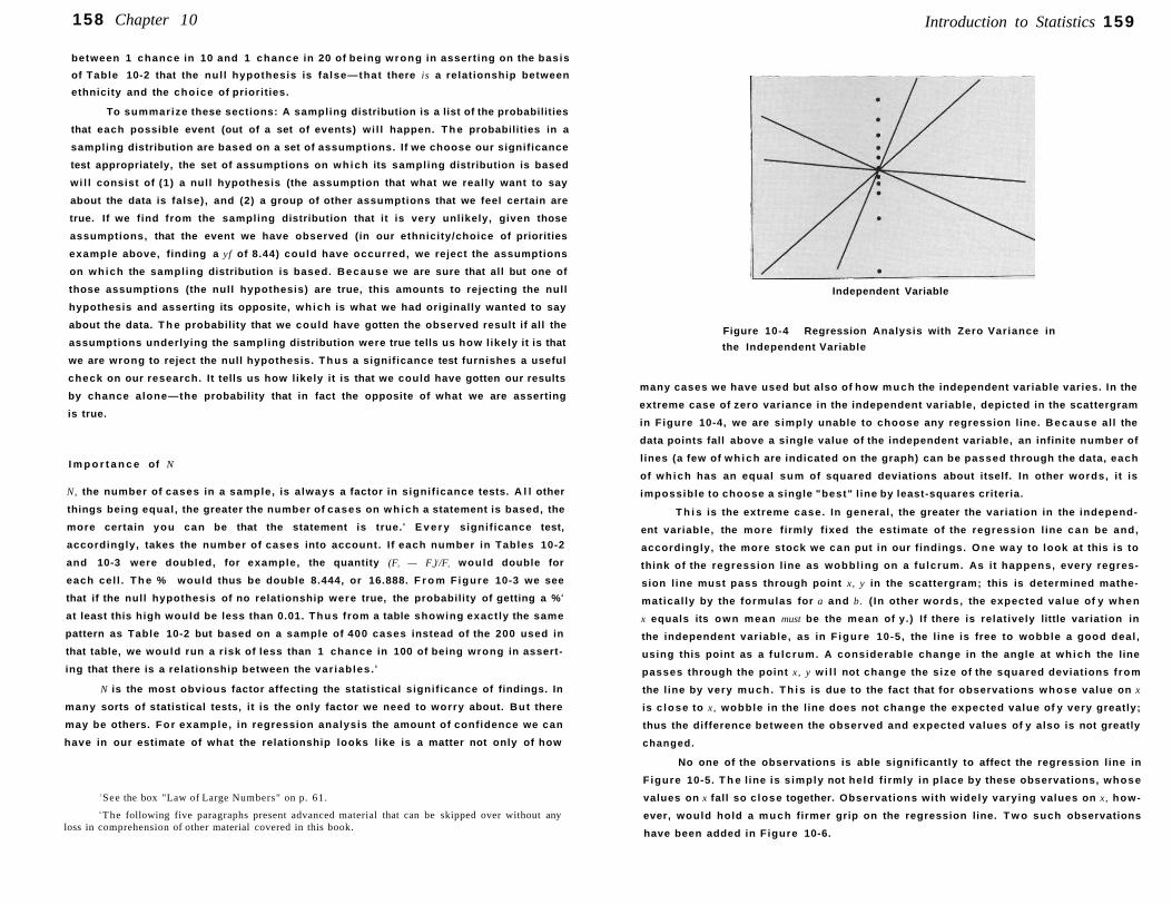
158 Chapter 10

between 1 chance in 10 and 1 chance in 20 of being wrong in asserting on the basis

of Table 10-2 that the nul l hypothesis is fa lse—that there is a relationship between

ethnicity and the choice of priorities.

To summarize these sections: A sampling distribution is a list of the probabilities

that each possible event (out of a set of events) wi l l happen. T h e probabilities in a

sampling distribution are based on a set of assumptions. If we choose our significance

test appropriately, the set of assumptions on wh ich its sampling distribution is based

wi l l consist of (1) a null hypothesis (the assumption that what we really want to say

about the data is false), and (2) a group of other assumptions that we feel certain are

true. If we find from the sampling distribution that it is very unlikely, given those

assumptions, that the event we have observed (in our ethnicity/choice of priorities

example above, finding a yf of 8.44) could have occurred, we reject the assumptions

on which the sampling distribution is based. Because we are sure that all but one of

those assumptions (the null hypothesis) are true, this amounts to rejecting the null

hypothesis and asserting its opposite, wh ich is what we had originally wanted to say

about the data. T h e probability that we could have gotten the observed result if all the

assumptions underlying the sampling distribution were true tells us how l ikely it is that

we are wrong to reject the null hypothesis. T h u s a significance test furnishes a useful

check on our research. It tells us how likely it is that we could have gotten our results

by chance alone—the probability that in fact the opposite of what we are asserting

is true.

I m p o r t a n c e of N

N, the number of cases in a sample, is a lways a factor in signif icance tests. A l l other

things being equal, the greater the number of cases on w h i c h a statement is based, the

more certain you can be that the statement is true. 5 E v e r y signif icance test,

accordingly, takes the number of cases into account. I f each number in Tables 10-2

and 10-3 were doubled, for example, the quantity (F0 — Fh)2/Fh would double for

each cel l . T h e % would thus be double 8.444, or 16.888. F r o m F igure 10-3 we see

that if the null hypothesis of no relationship were true, the probability of getting a % 2

at least this high would be less than 0.01. T h u s from a table showing exactly the same

pattern as Table 10-2 but based on a sample of 400 cases instead of the 200 used in

that table, we would run a risk of less than 1 chance in 100 of being wrong in assert­

ing that there is a relationship between the var iables. 6

N is the most obvious factor affecting the statistical signif icance of findings. In

many sorts of statistical tests, it is the only factor we need to worry about. But there

may be others. For example, in regression analysis the amount of confidence we can

have in our estimate of what the relationship looks l ike is a matter not only of how

5 See the box "Law of Large Numbers" on p. 61. 6 The following five paragraphs present advanced material that can be skipped over without any

loss in comprehension of other material covered in this book.

Introduction to Statistics 159

Independent Variable

Figure 10-4 Regression Analysis with Zero Variance in

the Independent Variable

many cases we have used but also of how much the independent variable varies. In the

extreme case of zero variance in the independent variable, depicted in the scattergram

in Figure 10-4, we are simply unable to choose any regression line. B e c a u s e all the

data points fall above a single value of the independent variable, an infinite number of

l ines (a few of w h i c h are indicated on the graph) can be passed through the data, each

of wh ich has an equal sum of squared deviations about itself. In other words, it is

impossible to choose a single "best" l ine by least-squares criteria.

T h i s is the extreme case. In general , the greater the variation in the independ­

ent variable, the more firmly fixed the estimate of the regression l ine can be and,

accordingly, the more stock we can put in our f indings. O n e w a y to look at this is to

think of the regression line as wobbl ing on a fu lcrum. As it happens, every regres­

sion l ine must pass through point x, y in the scattergram; this is determined mathe­

matical ly by the formulas for a and b. ( In other words, the expected value of y when

x equals its own mean must be the mean of y.) If there is relatively little variation in

the independent variable, as in F igure 10-5, the l ine is free to wobble a good deal ,

using this point as a fu lcrum. A considerable change in the angle at wh ich the line

passes through the point x, y w i l l not change the size of the squared deviations f rom

the l ine by very much . T h i s is due to the fact that for observations whose value on x

is c lose to x, wobble in the l ine does not change the expected value of y very greatly;

thus the difference between the observed and expected values of y also is not greatly

changed.

No one of the observations is able significantly to affect the regression line in

F igure 10-5. T h e l ine is s imply not held f irmly in place by these observations, whose

values on x fall so c lose together. Observations with widely varying values on x, how­

ever, would hold a much firmer grip on the regression line. T w o such observations

have been added in Figure 10-6.

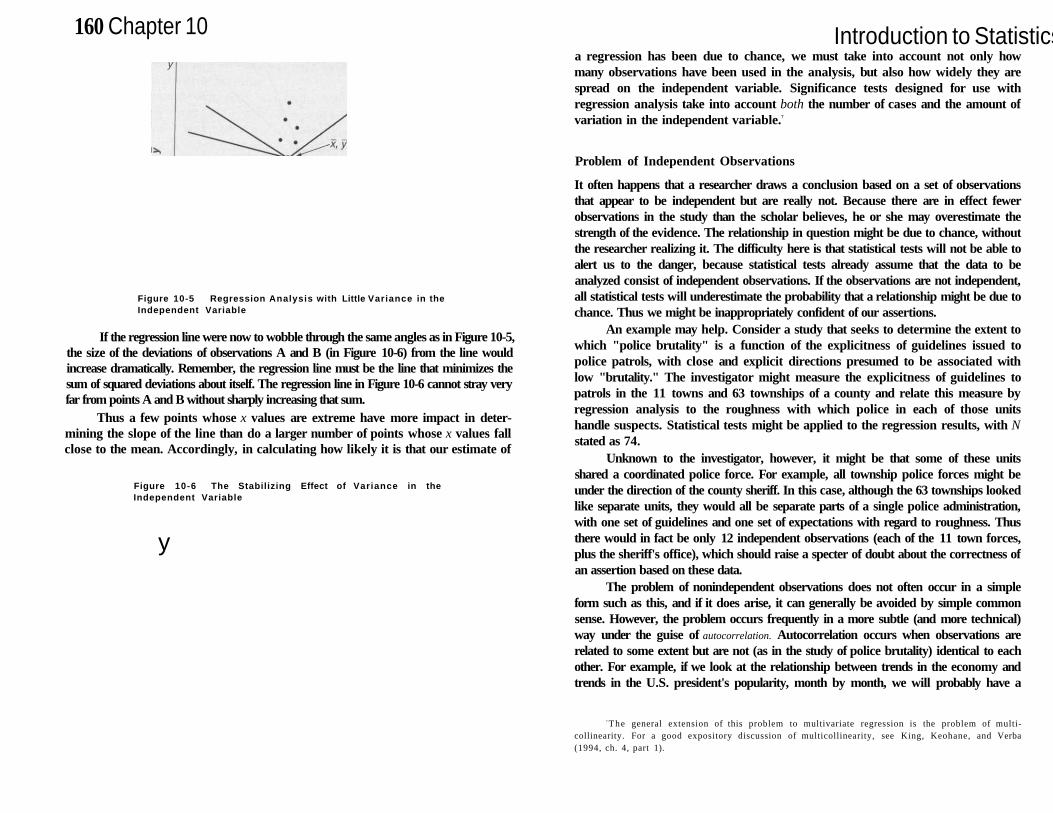
160 Chapter 10

Figure 10-5 Regression Analysis with Little Variance in the Independent Variable

If the regression line were now to wobble through the same angles as in Figure 10-5, the size of the deviations of observations A and B (in Figure 10-6) from the line would increase dramatically. Remember, the regression line must be the line that minimizes the sum of squared deviations about itself. The regression line in Figure 10-6 cannot stray very far from points A and B without sharply increasing that sum.

Thus a few points whose x values are extreme have more impact in deter­mining the slope of the line than do a larger number of points whose x values fall close to the mean. Accordingly, in calculating how likely it is that our estimate of

Figure 10-6 The Stabilizing Effect of Variance in the Independent Variable

y

Introduction to Statistics 161 a regression has been due to chance, we must take into account not only how many observations have been used in the analysis, but also how widely they are spread on the independent variable. Significance tests designed for use with regression analysis take into account both the number of cases and the amount of variation in the independent variable.7

Problem of Independent Observations

It often happens that a researcher draws a conclusion based on a set of observations that appear to be independent but are really not. Because there are in effect fewer observations in the study than the scholar believes, he or she may overestimate the strength of the evidence. The relationship in question might be due to chance, without the researcher realizing it. The difficulty here is that statistical tests will not be able to alert us to the danger, because statistical tests already assume that the data to be analyzed consist of independent observations. If the observations are not independent, all statistical tests will underestimate the probability that a relationship might be due to chance. Thus we might be inappropriately confident of our assertions.

An example may help. Consider a study that seeks to determine the extent to which "police brutality" is a function of the explicitness of guidelines issued to police patrols, with close and explicit directions presumed to be associated with low "brutality." The investigator might measure the explicitness of guidelines to patrols in the 11 towns and 63 townships of a county and relate this measure by regression analysis to the roughness with which police in each of those units handle suspects. Statistical tests might be applied to the regression results, with N stated as 74.

Unknown to the investigator, however, it might be that some of these units shared a coordinated police force. For example, all township police forces might be under the direction of the county sheriff. In this case, although the 63 townships looked like separate units, they would all be separate parts of a single police administration, with one set of guidelines and one set of expectations with regard to roughness. Thus there would in fact be only 12 independent observations (each of the 11 town forces, plus the sheriff's office), which should raise a specter of doubt about the correctness of an assertion based on these data.

The problem of nonindependent observations does not often occur in a simple form such as this, and if it does arise, it can generally be avoided by simple common sense. However, the problem occurs frequently in a more subtle (and more technical) way under the guise of autocorrelation. Autocorrelation occurs when observations are related to some extent but are not (as in the study of police brutality) identical to each other. For example, if we look at the relationship between trends in the economy and trends in the U.S. president's popularity, month by month, we will probably have a

7 The general extension of this problem to multivariate regression is the problem of multi-collinearity. For a good expository discussion of multicollinearity, see King, Keohane, and Verba (1994, ch. 4, part 1).

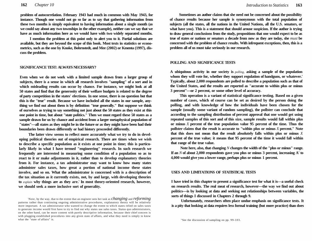
162 Chapter 10

problem of autocorrelation. February 1943 had much in common with May 1943, for instance. Though one would not go so far as to say that gathering information from these two months is simply equivalent to having information about a single month (as we could say about any two townships in the other example), neither can we say that we have as much information here as we would have with two widely separated months.

I mention the problem at this point only to alert you to it. Partial solutions are available, but they are beyond the scope of this book. Most texts in statistics or econo­metrics, such as the one by Knoke, Bohrnstedt, and Mee (2002) or Kmenta (1997), dis­cuss the problem.

SIGNIFICANCE TEST: ALWAYS NECESSARY?

Even when we do not work with a limited sample drawn from a larger group of subjects, there is a sense in which all research involves "sampling" of a sort and in which misleading results can occur by chance. For instance, we might look at all 50 states and find that the generosity of their welfare budgets is related to the degree of party competition in the states' elections. In one sense, there is no question but that this is the "true" result. Because we have included all the states in our sample, any­thing we find out about them is by definition "true generally." But suppose we think of ourselves as trying to say something not just about the 50 states as they exist at this one point in time, but about "state politics." Then we must regard these 50 states as a sample drawn for us by chance and accident from a larger metaphysical population of "states"—all states as they might be in the future or as they might have been had their boundaries been drawn differently or had history proceeded differently.

The latter view seems to reflect more accurately what we try to do in devel­oping political theories out of empirical research. There are times when we wish to describe a specific population as it exists at one point in time; this is particu­larly likely in what I have termed "engineering" research. In such research we frequently are interested in measuring some condition of a population so as to react to it or make adjustments in it, rather than to develop explanatory theories from it. For instance, a tax administrator may want to know how many states administer sales taxes, how great a portion of national income these states involve, and so on. What the administrator is concerned with is a description of the tax situation as it currently exists, not, by and large, with developing theories to explain why things are as they are.8 In most theory-oriented research, however, we should seek a more inclusive sort of generality.

8 Note, by the way, that to the extent that an engineer sees her task as changing and reforming patterns rather than continuing ongoing administrative procedures, explanatory theory will be relatively more important. A tax administrator who wanted to change the extent to which states relied on sales taxes to generate income would first have to try to find out why states use sales taxes. Status quo administrators, on the other hand, can be more content with purely descriptive information, because their chief concern is with plugging established procedures into any given state of affairs, and what they need is simply to know what the "state of affairs" is.

Introduction to Statistics 163

Sometimes an author claims that she need not be concerned about the possibility of chance results because her sample is synonymous with the total population of subjects (all the states, all the nations in the United Nations, all the U.S. senators, or what have you). This is a statement that should arouse suspicion. If the author is trying to draw general conclusions from the study, propositions that one would expect to be as true of states or nations or senators a decade from now as they are today, she must be concerned with the problem of chance results. With infrequent exceptions, then, this is a problem all of us must take seriously in our research.

POLLING AND SIGNIFICANCE TESTS

A ubiquitous activity in our society is polling, asking a sample of the population whom they will vote for, whether they support regulation of handguns, or whatever.9

Typically, about 2,000 respondents are polled to describe a population such as that of the United States, and the results are reported as "accurate to within plus or minus 3 percent"—or 2 percent, or some other level of accuracy.

This operation is a variant of statistical significance testing. Based on a given number of cases, which of course can be set as desired by the person doing the polling, and with knowledge of how the individuals have been chosen for the sample (usually some variant of random sampling), the pollster can conclude that according to the sampling distribution of percent approval that one would get using repeated samples of this sort and of this size, sample results would fall within plus or minus X percent of the true population value 95 percent of the time. Thus the pollster claims that the result is accurate to "within plus or minus X percent." Note that this does not mean that the result absolutely falls within plus or minus X percent of the true value; it means that 95 percent of the time it would fall within that range of the true value.

Note here, also, that changing N changes the width of the "plus or minus" range. If an N of about 2,000 respondents gave you plus or minus 3 percent, increasing A' to 4,000 would give you a lower range, perhaps plus or minus 1 percent.

USES AND LIMITATIONS OF STATISTICAL TESTS

I have tried in this chapter to present a significance test for what it is—a useful check on research results. The real meat of research, however—the way we find out about politics—is by looking at data and seeking out relationships between variables, the sorts of things I discussed in Chapters 2 through 9.

Unfortunately, researchers often place undue emphasis on significance tests. It is a pity that looking at data requires less formal training (but more practice) than does

''See the discussion of sampling on pp. 99-103.

164 Chapter 10

calculating significance tests. Perhaps because they have spent so much time in cours­es learning to use significance tests, many researchers give the tests an undue empha­sis in their research. The status of these tests should be strictly that of a secondary check on the creative work the researcher has done in looking at relationships.

A recent article illustrates the problem. In this study, the authors reported that two variables were more strongly related among the working-class portion of their sample than among the middle-class portion. Their evidence for this was that among the working-class respondents, the relationship was more highly significant, with a probability of less than 0.01 that there was no relationship. Among the middle-class respondents, by contrast, the relationship was less highly significant, with probability between 0.01 and 0.05. Because previous theorists had said that one should expect a stronger relationship between these variables among the middle class than among the working class, these authors were understandably excited about their findings.

Unfortunately, they were using significance tests for something the tests were not meant to do. The significance test is not itself a measure of the strength of a relationship but rather, a check on how likely it is that a given measure is due to chance. In this example, as it happened, the middle-class portion of the authors' sample was only about half as large as the working-class portion. It was because of the smaller number of cases in the middle-class portion that its relationship showed up as less significant than the same relationship for the working-class portion. In fact, when the strength of the relationship was measured by an appropriate technique (the Goodman-Kruskal gamma, for instance), it turned out that there was a Wronger relationship among the middle class. The authors' conclusion from their own data was wrong.

CONCLUSION

I have tried in this chapter to give you some idea of the general logic of inference, which is the common thread running through all statistical tests. These tests vary among themselves, however, in terms of their suitability for a given level of measurement and the particular mix of assumptions (other than the null hypothesis) they require the investigator to guarantee. This is why there are so many different tests. For a description of particular tests, the reader should consult a statistics text such as the one cited at the end of Chapter 8.

FURTHER DISCUSSION

A particularly good discussion of the misapplication of significance tests, along the lines of the example I used, is Duggan and Dean, "Common Misinterpretations of Significance Levels in Sociological Journals" (1968). See also Winch and Campbell, "Proof? No. Evidence? Yes. The Significance of Tests of Significance" (1969).

Introduction to Statistics

Anyone thinking of using these tests should first take a course in statistics; barring that, however, useful presentations of the techniques are given in the text cited at the end of Chapter 8. The second chapter of Siegel (1956) is a particularly useful review of the overall logic of significance tests. It aims at much the same presentation as I have attempted in this chapter, but in rather more technical detail. Another very good treatment is that of Simon (1985).

For further consideration, think about the two following situations. What is wrong in each situation ?

1. A researcher studying Congress examines the vote on 100 or so bills. For two of these

votes, she finds a statistically significant relationship (at the 0.05 level) between a

representative's height and the way he voted on the bill. This strikes her as a surprising

finding, and she uses it as the basis for a chapter and a half of her book.

2. A large number of scholars study committee systems to see whether democracy in

committee decision making leads the members to be satisfied with their work on the

committee. All but one of these scholars fail to find a statistically significant relationship

between these two variables. Most of those who fail to find a relationship leave that

question and start to work on other things. A few of them write up their results, but these

are rejected by journal editors because they are negative, not positive, findings. The one

scholar who did find a statistically significant result publishes it. Net result: one published

article, reporting a statistically significant relationship between committee democracy

and members' satisfaction.

Chapter 11

®d4 ©DTTD1

Lr®LnjTj 9 o

T h i s h a s b e e n a b o o k a b o u t d e v e l o p i n g t h e o r i e s a n d t r y i n g t h e m o u t o n r e a l i t y .

I n C h a p t e r 2 , I e q u a t e d t h e r e s e a r c h p r o c e s s w i t h a s e a r c h f o r e l e g a n t t h e o r i e s . I n

s u c c e e d i n g c h a p t e r s , I h a v e d i s c u s s e d v a r i o u s a s p e c t s o f r e s e a r c h : c o n c e p t f o r m a t i o n ,

m e a s u r e m e n t , d a t a a n a l y s i s . M y c r i t e r i o n fo r t h e u s e f u l n e s s o f a n y o f t h e s e t e c h n i q u e s

h a s b e e n t h e e x t e n t t o w h i c h t h a t t e c h n i q u e a i d e d i n t h e c r e a t i o n o f e l e g a n t t h e o r i e s .

A h i g h d e g r e e o f " p r e c i s i o n i n m e a s u r e m e n t " i s i m p o r t a n t , I h a v e a r g u e d , b e c a u s e i t

a l l o w s u s m o r e f l e x i b i l i t y i n s t a t i n g t h e theory w e c h o o s e t o w o r k w i t h . M e a s u r e m e n t

a c c u r a c y , w h e t h e r i t i s a m a t t e r o f r e l i a b i l i t y o r v a l i d i t y , i s i m p o r t a n t b e c a u s e w i t h o u t

a c c u r a t e m e a s u r e m e n t w e c a n n o t e s t a b l i s h t h e c o n n e c t i o n b e t w e e n t h e d a t a w e a r e

h a n d l i n g a n d t h e theory w i t h w h i c h w e a r e w o r k i n g . R e g r e s s i o n a n a l y s i s u s u a l l y i s

m o r e u s e f u l t h a n c o r r e l a t i o n a n a l y s i s , b e c a u s e t h e r e s u l t s o f r e g r e s s i o n a n a l y s i s a p p l y

g e n e r a l l y t o a theory, w h e r e a s t h e r e s u l t s o f c o r r e l a t i o n a n a l y s i s c a n s e r v e o n l y a s a

d e s c r i p t i o n o f a p a r t i c u l a r s i t u a t i o n ; a n d s o o n .

I n a l l o f t h i s , I h a v e n e v e r d e a l t w i t h t h e c r i t i c a l q u e s t i o n : J u s t h o w d o e s o n e f ind

a t h e o r y o n w h i c h t o w o r k ? T h e r e i s o n e d e c e p t i v e l y s i m p l e a n s w e r t o t h i s q u e s t i o n ,

w h i c h i s t o c h o o s e t h e o r i e s fo r s t u d y f r o m t h e a l r e a d y e x i s t i n g b o d y o f w o r k i n p o l i t i ­

c a l s c i e n c e . T h a t i s , t a k e a n e x i s t i n g t h e o r y a n d t ry i t o u t o n s o m e d a t a . I d i s c u s s e d

s o m e o f t h e l i m i t a t i o n s o f t h i s p r o c e d u r e i n C h a p t e r 2 , b u t t h e i m p o r t a n t p o i n t fo r m y

d i s c u s s i o n h e r e i s t h a t t h i s a n s w e r b e g s t h e q u e s t i o n o f h o w t h e o r i g i n a l t h e o r i s t f o u n d

t h e t h e o r y .

W h a t m a k e s a p o l i t i c a l s c i e n t i s t d e s c r i b e t h e r e l a t i o n s h i p a m o n g a g r o u p o f

v a r i a b l e s i n a p a r t i c u l a r w a y ? P r o b a b l y i t m o s t f r e q u e n t l y h a p p e n s t h a t t h e

r e s e a r c h e r o b s e r v e s a b o d y o f d a t a a n d t r i e s t o s e e a p a t t e r n a m o n g t h e m . T h i s i s

t h e m o s t o b v i o u s w a y t o g o a b o u t d e v i s i n g a t h e o r y ; i t f o l l o w s q u i t e n a t u r a l l y f r o m

t h e t h i n g s a t h e o r y i s s u p p o s e d t o a c h i e v e . T h e p u r p o s e o f a t h e o r y i s t o p r o v i d e a

s i m p l i f i e d p a t t e r n t o d e s c r i b e a c o m p l i c a t e d j u m b l e o f o b s e r v a t i o n s . W o u l d i t n o t

166

Where Do Theories Come From? 167

f o l l o w , t h e n , t h a t t h e m o s t a p p r o p r i a t e w a y t o d e v i s e a t h e o r y i s s i m p l y t o l o o k a t

t h e j u m b l e o f o b s e r v a t i o n s a n d p i c k o u t t h e m o s t p r o m i n e n t p a t t e r n r u n n i n g

t h r o u g h t h e m ?

U n f o r t u n a t e l y , " o b s e r v a t i o n s " i n p o l i t i c a l s c i e n c e a r e r i d d l e d w i t h p r o b l e m s o f

i n a c c u r a t e m e a s u r e m e n t ; t h e y a r e o f t e n m e a s u r e d i m p r e c i s e l y , a n d t h e n o n e x p e r i -

m e n t a l c i r c u m s t a n c e s u n d e r w h i c h w e g a t h e r t h e m m a k e i t d i f f i c u l t t o i s o l a t e t h e

e f f e c t s o f s i n g l e v a r i a b l e s . T h e s e a r e a l l p r o b l e m s I d i s c u s s e d e a r l i e r i n t h e b o o k .

T h e i r c o m b i n e d e f f e c t i s t o m a k e i t v e r y d i f f i c u l t t o l o o k a t a b a t c h o f o b s e r v a t i o n s

a n d p i c k o u t t h e b e s t s i m p l i f y i n g p a t t e r n . T h e r e i s s o m u c h g o i n g o n i n a g r o u p o f

o b s e r v a t i o n s , m u c h o f w h i c h i s e x t r a n e o u s t o w h a t w e w a n t t o d o , t h a t t h e p a t t e r n w e

i d e a l l y w o u l d h o p e t o p i c k o u t i s o b s c u r e d .

T h i s p r o b l e m i s n o t c o n f i n e d t o t h e s o c i a l s c i e n c e s . A n a m u s i n g e x a m p l e o f

t h e d i f f i c u l t y o f c h o o s i n g a m o n g p o t e n t i a l e x p l a n a t i o n s w i t h o u t t h e b e n e f i t o f p r i o r

t h e o r y i s o f f e r e d b y a d i s c u s s i o n a m o n g S a m u e l J o h n s o n , J a m e s B o s w e l l , a n d

s o m e o f t h e i r f r i e n d s i n 1 7 6 9 a b o u t t h e m y s t e r y o f w h y t h e r e s i d e n t s o f t h e

S c o t t i s h i s l a n d o f S t . K i l d a c a u g h t c o l d w h e n e v e r a s h i p a r r i v e d t h e r e . 1 T h e r e w a s

a t t h a t t i m e a l r e a d y s p e c u l a t i o n t h a t i l l n e s s e s w e r e t r a n s m i t t e d f r o m o n e p e r s o n t o

a n o t h e r , b u t J o h n s o n r e g a r d e d t h i s a s a " p r e j u d i c e , " a n d n o t " s m a r t m o d e r n

t h o u g h t . " E v e n t u a l l y t h e e x p l a n a t i o n f a v o r e d b y B o s w e l l w a s o f f e r e d i n a l e t t e r

f r o m a L a d y o f N o r f o l k :

Now for the explication of this seeming mystery, which is so very obvious as, for

that reason, to have escaped the penetration of Dr. Johnson and his friend, as well

as that of the author. Reading the book with my ingenious friend, the late Reverend

Mr. Christian, of Docking—after ruminating a little, "The cause, (says he,) is a

natural one. The situation of St. Ki lda renders a North-East Wind indispensably

necessary before a stranger can land. The wind, not the stranger, occasions an epi­

demic cold."

I n a s i m i l a r v e i n , J a m e s S . C o l e m a n d e s c r i b e d t h e w a y t h e t h e o r y o f g r a v i t y

m i g h t not h a v e b e e n d e v i s e d h a d G a l i l e o g o n e a b o u t h i s t a s k i n t h e w a y m o s t d a t a -

a n a l y z i n g s o c i a l s c i e n t i s t s d o :

A simple example will illustrate some of the difficulties which might arise by this

kind of "brick-by-brick" approach to theory. Suppose that early mechanics had

developed by the use of regression equations. Suppose, specifically, that an investiga­

tion had been carried out relating the length of time a body had fallen through the air

and the velocity it attained. The relation in mechanics is that the velocity attained is

equal to the acceleration due to gravity times the time the object has fallen, or

v = gt

'G. Birkbeck Hill, Be/swell's Life of Johnson, Vol. 2 (London: Clarendon Press, 1887), pp. 51-52. 2 lb id . ,p . 52.

168 Chapter 11

where g is the acceleration due to gravity. Now if there had been numerous investiga­

tions involving different-sized bodies, different velocities, and bodies with differing

densities, the investigators would have ended with numerous pairs of observations

( V j , tt), which they would locate on a scatter diagram in order to find the line of best

fit. But in every case, and especially for high velocities (i.e., objects which fell a great

distance) and low-density objects (i.e., feathers), the observed velocity would fall

considerably below that which the theoretical equation predicts. The resulting regres­

sion equation might have ended up including other variables, such as mass or density

of the object; and there would have been indications that at high velocities the

relation of velocity to time was not even linear. The reason, of course, would be air

resistance, which has different effects as a function of the density of the object, its

shape, its velocity, and other things. The regression equation would of course have

been empirically correct, but it wouldn't have corresponded to the simple

velocity-time relation which served as the basis for Galileo's remarkable contribu­

tion to the science of mechanics. They might even have served to confound the issue,

by bringing in too soon a factor—i.e., air resistance—which was irrelevant to the

fundamentals of mechanics. 3

T h e m o r a l o f t h e s e s t o r i e s i s t h a t w e a l m o s t a l w a y s a r e b e t t e r off i f w e h a v e

s o m e i d e a o f w h a t k i n d o f p a t t e r n w e w a n t t o l o o k fo r b e f o r e w e s t a r t t o l o o k a t d a t a .

I f w e h a v e i n m i n d a p a r t i c u l a r k i n d o f p a t t e r n , i t i s e a s y t o t e l l , a m o n g t h e j u m b l e o f

t h i n g s w e f i nd , w h a t i s r e l e v a n t t o t h a t p a t t e r n a n d w h a t i s e x t r a n e o u s . G a l i l e o w a s

a b l e t o i g n o r e t h e e f f e c t s o f a i r r e s i s t a n c e b e c a u s e h e k n e w t h a t t h e y w e r e n o t t h e

t h i n g h e s h o u l d u s e t o e x p l a i n t h e s p e e d o f f a l l i n g o b j e c t s .

T h e d i s t i n c t i o n h e r e i s b e t w e e n " i n d u c t i v e " a n d " d e d u c t i v e " t h e o r y b u i l d i n g .

T o b u i l d t h e o r y i n d u c t i v e l y , t h e r e s e a r c h e r s c a n s t h e o b s e r v a t i o n s , l o o k i n g fo r

p a t t e r n s . T o b u i l d t h e o r y d e d u c t i v e l y , t h e r e s e a r c h e r d e d u c e s ( f r o m s o m e t h i n g e l s e ,

s o m e p r i o r e x p e c t a t i o n s ) w h a t s o r t o f a p a t t e r n t o e x p e c t a n d t h e n l o o k s fo r i t a m o n g

t h e o b s e r v a t i o n s .

A c c o r d i n g t o t h e a r g u m e n t I h a v e p r e s e n t e d s o f a r i n t h i s c h a p t e r , d e d u c t i v e

t h e o r y b u i l d i n g i s c l e a r l y t h e b e t t e r o f t h e t w o . T h e p r o b l e m l i e s w i t h t h a t " s o m e t h i n g

e l s e " f r o m w h i c h t h e s t u d e n t i s s u p p o s e d t o d e d u c e t h e o r i e s . T h e r e s i m p l y a r e n o t

m a n y w e l l - e s t a b l i s h e d premises i n t h e s o c i a l s c i e n c e s f r o m w h i c h t o d e d u c e a n y t h i n g .

O n e w a y o f d i s t i n g u i s h i n g a n o n g o i n g " s c i e n c e " f r o m a " p r e - s c i e n c e " i s t h a t t h e

f o r m e r i n c l u d e s a g e n e r a l l y a g r e e d - u p o n b o d y o f a s s u m p t i o n s f r o m w h i c h m o s t o f i ts

t h e o r i e s c a n b e d e d u c e d ( K u h n , 1 9 6 2 ) . P o l i t i c a l s c i e n c e , s o c i o l o g y , a n d s i m i l a r s o c i a l

s c i e n c e s c a n n o t b e s a i d t o p o s s e s s s u c h a b o d y o f a s s u m p t i o n s .

L a c k i n g t h i s b a s e fo r d e d u c t i o n , i t i s h a r d t o a r g u e p a t l y t h a t t h e o r y b u i l d i n g

m u s t b e d o n e d e d u c t i v e l y . O n t h e o t h e r h a n d , i t i s i m p o r t a n t t o b e a r i n m i n d t h e

a d v a n t a g e s o f d e d u c t i o n , w h e r e i t i s f e a s i b l e . T h e r e a r e s o m e t r i c k s t h a t m a y h e i g h t ­

e n y o u r a w a r e n e s s o f s i t u a t i o n s i n w h i c h d e d u c t i o n i s f e a s i b l e . O n e o f t h e b e s t

s o u r c e s o f d e d u c t i v e t h e o r y i s a w e l l - e s t a b l i s h e d t h e o r y f r o m a n o t h e r f i e ld . T h e o r i e s

3 James S. Coleman, Introduction to Mathematical Sociology (New York: The Free Press, 1964), pp. 100-101. Copyright 1964 by the Free Press.

Where Do Theories Come From? 169

o f e p i d e m i c g r o w t h a n d p o p u l a t i o n d y n a m i c s , f r o m s u c h f i e l d s a s e p i d e m i o l o g y

a n d e c o l o g y , m a y s u g g e s t t h e o r i e s t o p o l i t i c a l s c i e n t i s t s o r s o c i o l o g i s t s . S o m a y

m i c r o e c o n o m i c t h e o r y ; a s n o t e d i n C h a p t e r 1 , r a t i o n a l c h o i c e t h e o r y d r a w n f r o m

m i c r o e c o n o m i c t h e o r y h a s b e e n p a r t i c u l a r l y f ru i t fu l f o r p o l i t i c a l s c i e n c e . A h e a l t h y

a w a r e n e s s o f m a j o r t h e o r i e s i n f i e l d s s u c h a s t h e s e , s o m e o f w h i c h a r e n o t a l l t h a t

c l o s e l y r e l a t e d t o o u r f i e l d , c a n b e a h e l p f u l s o u r c e o f t h e o r y .

T h e a r t o f b u i l d i n g a t h e o r y r e m a i n s i n f l u x i n p o l i t i c a l s c i e n c e — p a r t l y

d e d u c t i v e , b u t l a r g e l y i n d u c t i v e . T h e r e s u l t i n g c o n f u s i o n c a n b e b o t h e n j o y a b l e a n d

f ru i t f u l , b e c a u s e m o r e t h a n i n m o s t d i s c i p l i n e s , i t a l l o w s a p l a c e f o r e v e r y s o r t o f

i m a g i n a t i o n t o w o r k : l i t e r a r y i m a g i n a t i o n , s c i e n t i f i c i m a g i n a t i o n , m o r a l i m a g i n a ­

t i o n , m a t h e m a t i c a l i m a g i n a t i o n . I t i s i n t h i s s p i r i t t h a t I h a v e t r i e d t o s t r e s s t h e

" c r a f t " i n t h e " c r a f t o f p o l i t i c a l r e s e a r c h . "

ACHEN, CHRISTOPHER H. 1975. "Attitudes and the Survey Response," American Political Science Review, 69 (December), 1218-1231. . 1986. The Statistical Analysis of Quasi-experiments. Berkeley, Calif.: University of California Press. , and W. PHILLIPS SHIVELY. 1995. Cross-Level Inference. Chicago: University of Chicago Press.

ANSOLABEHERE, STEPHEN, ALAN GERBER, and JAMES M. SNYDER, JR. 2002. "Equal Votes, Equal Money:

Court-Ordered Redistricting and the Distribution of Public Expenditures in the American States," American Political Science Review, 96, 767-777'.

ASHER, HERBERT B. 1974. "Some Consequences of Measurement Error in Survey Data," American Journal of Political Science, 18 (May), 469^185.

BACHRACH, PETER, and MORTON BARATZ. 1962. "The Two Faces of Power," American Political Science

Review, 56 (December), 947-953. BARBER, JAMES D. 1972. The Presidential Character: Predicting Performance in the White House. Upper

Saddle River, N.J.: Prentice Hall. BARTELS, LARRY M. 1993. "Messages Received: The Political Impact of Media Exposure," American

Political Science Review, 87 (June), 267-285. BARTON, ALLAN H. 1955. "The Concept of Property-Space in Social Research." In Paul F. Lazarsfeld and

Morris Rosenberg, eds., The Language of Social Research, pp. 40-53 . New York: Free Press. BATALLA, JAVIER ORTIZ. 1993. "Essays on the Early History of Latin American Central Banking," Ph.D.

dissertation in economics, University of California-Los Angeles. BERNSTEIN, RICHARD J. 1978. Restructuring of Social and Political Theory. Philadelphia: University of

Pennsylvania Press. BLALOCK, HUBERT M. 1964. Causal Inferences in Nonexperimental Research. Chapel Hill, N.C.:

University of North Carolina Press. . 1969. Theory Construction: Prom Verbal to Mathematical Formulations. Upper Saddle River, N.J.: Prentice Hall. . 1979. Social Statistics, rev. 2nd ed. New York: McGraw-Hill.

BRUNNER, RONALD D. 1977. "An 'Intentional' Alternative in Public Opinion Research," American Journal of Political Science, 21 (August), 435-464.

BUENO DE MESQUITA, BRUCE, JAMES D. MORROW, RANDOLPH M. SIVERSON, and ALASTAIR SMITH. 1999.

"An Institutional Explanation of the Democratic Peace," American Political Science Review, 93 (December), 791-808.

BUTLER, DAVID, and DONALD STOKES. 1969. Political Change in Britain. New York: St. Martin's Press. CAMPBELL, ANGUS, and others. 1960. The American Voter. New York: John Wiley & Sons.

170

Selected Bibliography 171

CAMPBELL, DONALD T, and JULIAN C. STANLEY. 1963. Experimental and Quasi-experimental Designs for

Research. Chicago: Rand McNally. CARTER, LEWIS F. 1971. "Inadvertent Sociological Theory," Social Forces, 50, 12-25. COLEMAN, JAMES S. 1964. Introduction to Mathematical Sociology. New York: Free Press. CONVERSE, PHILIP E. 1964. "The Nature of Belief Systems in Mass Publics." In David Apter, ed., Ideology

and Discontent, pp. 206-261. New York: Free Press. . 1969. "Of Time and Partisan Stability," Comparative Political Studies, 2, 139-171. , and GEORGES DUPEUX. 1962. "Politicization of the Electorate in France and the United States," Public Opinion Quarterly, 26 (Spring), 1-23. , and ROY PIERCE. 1985. "Measuring Partisanship," Political Methodology, 11, 143—166.

COOK, THOMAS D., and DONALD T. CAMPBELL. 1979. Quasi-experimentation: Design and Analysis Issues

for Field Setting. Chicago: Rand McNally. DAHL, ROBERT. 1961. Who Governs! New Haven, Conn.: Yale University Press.

. 1966. Political Oppositions in Western Democracies. New Haven, Conn.: Yale University Press.

. 1984. Modern Political Analysis, 4th ed. Upper Saddle River, N.J.: Prentice Hall. DALTON, RUSSELL J., and STEVEN WELDON. 2007. "Partisanship and Party System Institutionalization,"

Party Politics, 13, 179-196. DIEHL, PAUL F, and JEAN KINGSTON. 1987. "Messenger or Message? Military Buildups and the Initiation

of Conflict," Journal of Politics, 49 (August), 801-813. DIGESER, PETER. 1992. "The Fourth Face of Power," Journal of Politics, 54 (November), 977-1007. DOWNS, ANTHONY. 1957. An Economic Theory of Democracy. New York: Harper & Row. DRAPER, N. R., and H. SMITH. 1981. Applied Regression Analysis, 2nd ed. New York: John Wiley

& Sons. DUGGAN, THOMAS J., and CHARLES W. DEAN. 1968. "Common Misinterpretations of Significance Levels

in Sociological Journals," American Sociologist, 3 (February), 45^16. DUVERGER, MAURICE. 1963. Political Parties. New York: Science Editions. ECKSTEIN, HARRY. 1960. Pressure Group Politics. London: George Allen & Unwin.

. 1966. Division and Cohesion in Democracy. Princeton, N.J.: Princeton University Press. EDWARDS, ALLEN L. 1973. Statistical Methods, 3rd ed. New York: Holt, Rinehart & Winston. FELDMAN, STANLEY. 1983. "The Measurement and Meaning of Trust in Government," Political

Methodology, 9, 341-354. GEDDES, BARBARA. 2003. Paradigms and Sand Castles: Theory Building and Research Design in

Comparative Politics. Ann Arbor: University of Michigan Press. GERBER, ALAN S., and DONALD P. GREEN. 2000. "The Effects of Personal Canvassing, Telephone Calls,

and Direct Mail on Voter Turnout: A Field Experiment," American Political Science Review, 94 (September), 653-664.

GERRING, JOHN. 2007. Case Study Research: Principles and Practices. New York: Cambridge University Press.

GILBERT, JOHN P., RICHARD J. LIGHT, and FREDERICK MOSTELLER. 1975. "Assessing Social Innovations: An

Empirical Basis for Policy." In Carl A. Bennett and Arthur A. Lumsdaine, eds., Evaluation and Experiment, pp. 39-193. New York: Academic Press.

GOLDSMITH, ARTHUR A. 1987. "Does Political Stability Hinder Economic Development?" Comparative Politics, 19,471^180.

GOODMAN, LEO A., and WILLIAM H. KRUSKAL. 1954. "Measures of Association for Cross Classifications,"

Journal of the American Statistical Association, 49 (December), 747-754. GREEN, DONALD, and ALAN GERBER, eds. 2004. American Behavioral Scientists, 48, 1 (January). GREENSTEIN, FRED I. 2000. The Presidential Difference: Leadership and Style from FDR to Clinton.

New York: Free Press. HAMMOND, THOMAS H., and JANE M. FRASER. 1984. "Studying Presidential Performance in Congress,"

Political Methodology, 10, 211-244. HILDEBRAND, DAVID K., JAMES D. LAING, and HOWARD ROSENTHAL. 1977. Analysis of Nominal Data.

Beverly Hills, Calif.: Sage. HOWELL, WILLIAM G., PATRICK J. WOLF, DAVID E. CAMPBELL, and PAUL E. PETERSON, 1966. "Test-Score

Effects of School Vouchers in Dayton, Ohio, New York City, and Washington, D.C.: Evidence from Randomized Field Trials." Paper presented at the annual meetings of the American Political Science Association, Washington, D.C., September 2000. 2002. "School Vouchers and Academic Performance: Results from Three Randomized Field

Trials" Journal of Policy Analysis and Management, 21(2), 191-217.

172 Selected Bibliography

INTERNATIONAL INSTITUTE FOR STRATEGIC STUDIES. 2006. The Military Balance, 2006. Oxford: Oxford University Press.

IYENGAR, SHANTO, and DONALD R. KINDER. 1987. News That Matters. Chicago: University of Chicago Press. JACOB, PHILIP E. 1955. "A Multi-dimensional Classification of Atrocity Stories." In Paul F. Lazarsfeld

and Morris Rosenberg, eds., The Language of Social Research, pp. 54-57 . New York: Free Press.

KARSTEN, PETER, and others. 1971. "ROTC, Mylai and the Volunteer Army," Foreign Policy, 2 (Spring), 135-161.

KEY, V. O., JR. 1950. Southern Politics. New York: Alfred A. Knopf. KINDER, DONALD R., and THOMAS R. PALFREY, eds. 1993. Experimental Foundations of Political Science.

Ann Arbor, Mich.: University of Michigan Press. KING, GARY, ROBERT O. KEOHANE, and SIDNEY VERBA. 1994. Designing Social Inquiry: Scientific

Inference in Qualitative Research. Princeton, N.J.: Princeton University Press. KIRK, JEROME, and M A R C L. MILLER. 1985. Reliability and Validity in Qualitative Research. Beverly Hills,

Calif.: Sage. KMENTA, JAN. 1997. Elements of Econometrics, 2nd ed. Ann Arbor: University of Michigan Press. KNOKE, DAVID, GEORGE W. BOHRNSTEDT, and ALISSA POTTER M E E . 2002. Statistics for Social Data

Analysis, 4th ed. Belmont, Calif.: Wadsworth. KOENIG, LOUIS W. 1968. The Chief Executive, rev. ed. New York: Harcourt Brace Jovanovich. KOESTLER, ARTHUR. 1969. The Act of Creation. London: Hutchinson.

KROEBER, A. L., and CLYDE KLUCKHOHN. 1952. Culture: A Critical Review of Concepts and Definitions. Cambridge, Mass.: The Museum.

KUHN, THOMAS S. 1962. The Structure of Scientific Revolutions. Chicago: University of Chicago Press. LAVE, A. CHARLES, and JAMES G. MARCH. 1975. Introduction to Models in the Social Sciences. New York:

Harper & Row. LEITNER, CHRISTOPHER. 1997. "Of Time and partisan Stability Revisited: Australia and New Zealand

1905-90," American Journal of Political Science, 41 ,1104-1127. LUKES, STEVEN. 1974. Power: A Radical View. London: Macmillan. MASSEY, DOUGLAS S„ and KRISTIN E. ESPINOSA. 1997. "What's Driving Mexico-U.S. Migration?

A Theoretical, Empirical, and Policy Analysis," American Journal of Sociology, 102 (January), 939-999.

MATTHEWS, DONALD R., and JAMES W. PROTHRO. 1963. "Social and Economic Factors and Voter

Registration in the South," American Political Science Review, 57 (March), 24ff. MIHAELESCU, MIHAELA. 2004. "Interethnic Cooperation in Post-Communist Eastern Europe." Ph.D.

dissertation in political science, University of Minnesota, expected completion 2005. MOON, J. DONALD 1975. "The Logic of Political Inquiry: A Synthesis of Opposed Perspectives." In Fred

Greenstein and Nelson Polsby, eds., Handbook of Political Science, Vol. 1, pp. 131-228. Reading, Mass.: Addison-Wesley.

MOSTELLER, FREDERICK. 1968. "Errors," International Encyclopedia of the Social Sciences. New York: Macmillan.

NEUSTADT, RICHARD E. 1991. Presidential Power and the Modern Presidents. New York: Free Press. NIEMI, RICHARD G., and KEITH KREHBIEL. 1984. "The Quality of Surveying Responses About Parents and

the Family: A Longitudinal Analysis," Political Methodology, 10, 193-210. OLSON, MANCUR. 1965. The Logic of Collective Action. Cambridge, Mass.: Harvard University Press.

. 1982. The Rise and Decline of Nations. New Haven, Conn.: Yale University Press. OPPENHEIM, FELIX. 1975. "The Language of Political Inquiry: Problems of Clarification." In Fred

Greenstein and Nelson Polsby, eds., Handbook of Political Science, Vol. 1, pp. 283-336. Reading, Mass.: Addison-Wesley.

PITKIN, HANNA. 1967. The Concept of Representation. Berkeley, Calif.: University of California Press. . 1969. Representation. New York: Atherton.

PROTHRO, JAMES W. 1956. "The Nonsense Fight over Scientific Method: A Plea for Peace," Journal of Politics, 18, 565-570.

PRZEWORSKI, ADAM. 1975. "Institutionalization of Voting Patterns, or Is Mobilization the Source of Decay?" American Political Science Review, 69 (March), 49-67. , MICHAEL E. ALVAREZ, JOSE ANTONIO CHEIBUB, and FERNANDO LONGI. 2000. Democracy and

Development: Political Institutions and Well-Being in the World, 1950-1990. New York: Cambridge University Press.

PUTNAM, ROBERT D. 1993. Making Democracy Work. Cambridge, Mass.: Harvard University Press.

Selected Bibliography 173

REYNOLDS, H. T. 1977. Analysis of Nominal Data. Beverly Hills, Calif.: Sage. ROBINSON, W. S. 1950. "Ecological Correlations and the Behavior of Individuals," American Sociological

Review, 15 (June), 351-357. ROETHLISBERGER, F. J. , and W. J. DICKSON. 1939. Management and the Worker. Cambridge, Mass.:

Harvard University Press. ROGOWSKI, RONALD, and MARK ANDREAS KAYSER. 2002. "Majoritarian Electoral Systems and Consumer

Power: Price-Level Evidence from the OECD Countries," American Journal of Political Science, 46, 526-539.

SARTORI, GIOVANNI. 1976. Parties and Party Systems. London: Cambridge University Press. SHADISH, WILLIAM R., THOMAS D. COOK, and DONALD T . CAMPBELL. 2002. Experimental and Quasi-

Experimental Designs for Generalized Causal Inference. Boston: Houghton Mifflin. SHIVELY, W. PHILLIPS. 1972. "Party Identification, Party Choice, and Voting Stability: The Weimar Case,"

American Political Science Review, 66 (December), 1203-1225. . 2006. "Case Selection: Insights from Rethinking Social Inquiry',' Political Analysis, 14, 344-347.

SIEGEL, SIDNEY. 1956. Nonparametric Statistics for the Behavioral Sciences. New York: McGraw-Hill. SIMON, JULIAN. 1985. Basic Research Methods in Social Science, 3rd ed. New York: Random House. STOKES, DONALD E. 1969. "Cross-Level Inference as a Game Against Nature." In Joseph L. Bernd, ed.,

Mathematical Applications in Political Science, Vol. 4, pp. 62-83 . Charlottesville, Va.: The University of Virginia Press.

STOUFFER, SAMUEL, and others. 1949. The American Soldier, Vol. 1. Princeton, N.J.: Princeton University Press.

TARROW, SIDNEY. 1996. "Making Social Science Work Across Space and Time: A Critical Reflection on Robert Putnam's Making Democracy Work" American Political Science Review, 90 (June), 389-398. . 1971. "The Urban-Rural Cleavage in Political Involvement: The Case of France," American Political Science Review, 65 (June), 341-357.

TILLEY, JAMES R. 2003. "Party Identification in Britain: Does Length of Time in the Electorate Affect Strength of Partisanship?" British Journal of Political Science, 33, 332-344.

TINBERGEN, NIKO. 1968. Curious Naturalists. Garden City. N.Y.: Doubleday. TINGSTEN, HERBERT. 1937. Political Behavior. London: Longmans. TUFTE, EDWARD R. 1968-1969. "Improving Data Analysis in Political Science," World Politics, 21 ,

641-654. . 1983. The Visual Display of Quantitative Information. Cheshire, Conn.: Graphics Press.

UHLANER, CAROLE JEAN, and KAY LEHMAN SCHLOZMAN. 1986. "Candidate Gender and Congressional

Campaign Receipts," Journal of Politics, 48 (February), 30-50. VAN DETH, JAN W. 2000. "Interesting but Irrelevant: Social Capital and the Saliency of Politics in

Europe," European Journal of Political Science, 115-147. WATSON, JAMES D. 1968. The Double Helix. New York: Atheneum. W E B B , EUGENE J., DONALD T. CAMPBELL, RICHARD D. SCHWARTZ, and LEE SECHRIST. 1966. Unobtrusive

Measures. Chicago: Rand McNally. WILSON, THOMAS P. 1971. "Critique of Ordinal Variables." In Hubert M. Blalock, Jr., ed., Causal Models

in the Social Sciences, pp. 415^131. Chicago: Aldine-Atherton. WINCH, ROBERT E, and DONALD T. CAMPBELL. 1969. "Proof? No. Evidence? Yes. The Significance of

Tests of Significance," American Sociologist, 4 (May), 140-143. ZALLER, JOHN. 1998. "Politicians as Prize Fighters: Electoral Selection and Incumbency Advantage." In

John Geer, ed., Politicians and Party Politics. Baltimore: Johns Hopkins University Press.

Abstinence-only sex education, 81 Achen, Christopher H., 47, 87,

96, 128n Acton, Lord, 40 Alvarez, Michael E., 94, 110 Analytic political philosophy, 40 Anomalies, 29-30 Ansolabehere, Stephen, 54-55 Applied research, 4 Asher, Herbert B., 46n, 56 Autocorrelation, 161-162

B

Bachrach, Peter, 38 Baker v. Carr, 54n Baratz, Morton, 38 Barber, James David, 29 Bartels, Larry M., 131 Barton, Allan H., 40 Batalla, Javier Ortiz, 76 Bernstein, Richard J., 40 Blalock, Hubert M„ 96, 126,

127n, 146n Bohrnstedt, George W.,

131,162 Boswell, James, 167 Brunner, Ronald D., 31 Bueno de Mesquita, Bruce, 26-27 Butler, David, 20

Campbell, Angus, 18-19 Campbell, David E„ 87 Campbell, Donald T., 56, 85n,

96, 164 Carter, Lewis F., 73 Case studies, 103 Causal interpretations, 77-78

eliminating alternative, 78-84

Causation, 14, 74-76 Censored data, 103-106 Cheibub, Jose Antonio,

94, 110 Cluster sample, 101 Coefficient of determination, 124 Coleman, James S., 167-168 Continuous measures, 63-64 Control group, 80, 82

designs without, 79-81 Controlling for a variable,

94-95 Converse, Philip E., 17-20, 47,

56, 145 Cook, Thomas D„ 85, 96 Correlational measures of

relationship, 113 Correlation analysis, 122-127

compared with regression analysis, 127-130

Correlation coefficient, 123 Cross-tabulation, 132-134

174

Index 175

D

Dahl, Robert, 38, 40 Dalton, Russell J., 20 Dean, Charles W., 164 Dependent variable, 14 Dichotomies, 136-137

in regression analysis, 137-138 Dickson, W. J., 80n Diehl, Paul E, 8 Digeser, Peter, 38 Diminishing marginal returns model,

119-120 Discrete measures, 64 Downs, Anthony, 5-6 Duggan, Thomas J., 164 Duverger, Maurice, 2-3, 7n

E

Eckstein, Harry, 40, 57 Ecological fallacy, 128n Effect-descriptive measures of

relationship, 113 Elegant research, 16-17 Empirical research, 4 Engineering research, 5, 15, 23 English language, 32-33, 34 Epistemic correlation, 45n Espinosa, Kristin E., 16 Ethics of research, 11-12 Experiment, true, 83-84 Ex post facto argument, 23 Extrapolation, 49

F Face validity, 52 Feldman, Stanley, 56 Formal theory, 5-8 Fraser, Jane M., 56 Free rider problem, 7

G

Galileo, 167-168 Geddes, Barbara, 104-105

Gerber, Alan S., 54-55, 87, 96 Gerring, John, 110 Gilbert, John P., 87 Goldsmith, Arthur A., 30 Goodman, Leo A., 135n Goodman and Kruskal gamma, 135 Green, Donald P., 87, 96 Greenstein, Fred I., 29

H Hammond, Thomas H., 56 Hawthorne study, 80n Hill, G. Birkbeck, 167n Holding a variable constant,

76, 94-95 Howell, William G„ 87 Hypothesis testing, 151-153

I

Independence of observations, 161-162

Independent variable, 14 Interaction, statistical,

145-146, 146n Intercept of regression equation, 116 Interesting problems, 10 Interrupted time series, 90-91 Interval measures, 62 Iyengar, Shanto, 88

J Jacob, Philip E., 40 Johnson, Samuel, 167

K

Karsten, Peter, 69 Kayser, Mark Andreas, 86 Kemeny, John, 19 Keohane, Robert O., 110, 161n Key, V. O., Jr., 121-122 Kinder, Donald R., 87n, 88, 96

176 Index

King, Gary, 110, 161n

Kingston, Jean, 8

Kirk, Jerome, 56

Kluckhohn, Clyde, 38

Kmenta, Jan, 162

Knoke, David, 131, 162

Koenig, Louis W., 29

Koestler, Arthur, 31

Krehbiel, Keith, 56

Kroeber, A. L . , 38

Kruskal, William H., 135n

Kuhn, Thomas S. , 168

L Lave, Charles A. , 26n

Law of Large Numbers, 58, 61,

100, 106

Leitner, Christopher, 20

Liberal, 33

Light, Richard J . , 87

Linear relationships, 71,

118-119

Literary Digest, 50-51 Loewenberg, Gerhard, 109-110

Logit analysis, 139-141

Longi, Fernando, 94, 110

Lukes, Steven, 38

M

March, James G. , 26n

Markov chain, 19

Marx, Karl , 8

Massey, Douglas S. , 16

Matthews, Donald R., 144n

Measurement, general problem of,

42^15

Measurement error, 130-131

Mee, Alissa Potter, 131, 162

Mihaelescu, Mihaela, 99, 104

Mill , John Stuart, 5

Miller, Marc L. , 56

Minneapolis Star Tribune, 81

Moon, J. Donald, 31

Mosteller, Frederick, 56, 87

Multicollinearity, 161 n

Multidimensional concepts. 32

Multidimensional words, 34-35

Multivariate regression, 141-146

N

N (number of cases), 158-161

National Election Study, 101

National integration, 37

NATO, 25

Natural experiment, 82-83

without premeasurement, 83

Neustadt, Richard E . , 29

Niemi, Richard G. , 56

Nominal measures, 62

Nonempirical research, 4

Nonrandom error, 49, 53-54

Normative philosophy, 4-5

Null hypothesis, 152-153

o Olson, Mancur, 6-7, 26n, 30

Oppenheim, Felix, 40

Ordinal measures, 62

P

Palfrey, Thomas R„ 87n, 96

Peterson, Paul E . , 87

Pierce, Roy, 56

Pilot study, 51-52

Pitkin, Hanna, 40

Pluralism, 7

Political party, 33

Polling, 163

Power, 38-40

Precision, 58-67

and describing relationships between

variables, 65-67

enrichment of, 67-71

in measurement, 62-67

in measures, 58-61

Probit analysis, 139-141

Prothro, James W., 144n

Przeworski, Adam, 20, 94, 110

Index 111

Putnam, Robert D., 92-93

Puzzles, 25-28

Q Quantitative research, 20-21

R r, 123-127

r 2, 124, 126-127

Random error, 49, 53-54, 130-131

Random sample, 99-101

Ratio measures, 63n, 73

Rational choice, 6

R D D sampling, 101

Reagan, Ronald, 79

Recreational research, 4, 5-8

Regression analysis, 113-122

compared with correlation,

127-130

and measurement error, 130-131

Regression coefficient, 117

Regression to the mean, 88-90

Relative deprivation, 9

Reliability of measures, 45^18

related to validity, 49-50

Research design, 24, 78-84

Residuals, in regression, 119-122

Robinson, W. S . , 128n

Roethlisberger, F. J . , 80n

Rogowski, Ronald, 86

s Sampling, 99-102

purposive, 102

quasi-random, 101-102

random, 99-101

R D D , 101

Sampling distribution, 155-158

Sartori, Giovanni, 40

Scattergram, 113-114

Schlozman, Kay Lehman, 86

Schwartz, Richard D., 56

Sechrist, Lee, 56

Selection on the dependent variable

106-108

Shadish, William R., 96

Shively, W. Phillips, 20, 110n, I28n

Siegel, Sidney, 165

Significance, statistical, 149

Significance tests, 162-164

Simon, Julian, 165

Simplicity, of a theory, 15

Slope of regression equation, 116

Snyder, James M., 54-55

Social research, 2-3

Social status, 41-42

Split-half test for reliability, 47

Stanley, Julian C, 85n

Statistics, 112

Stokes, Donald E . , 20, 128n

Stouffer, Samuel, 9

Stratified sample, 60

T

Tarrow, Sidney, 29, 51, 52

Tsst group, 82

Test-retest check for reliability, 47

Theory, 2, 3, 14-17

Theory-oriented research, 8, 15, 23

Tilley, James R., 20

Tinbergen, Niko, 96

Tingsten, Herbert, 96

Topics for research, 22-23

Trivial theory, 15

True experiment, 83-84

Tufte, Edward R., 31,73

u Uhlaner, Carole Jean, 86

Unidimensional concepts, 32

Units, comparability in regression

analysis, 117

V

Validity, 48^19, 130-131

checking for, 51-53

Variables, 14

178 Index

Variance, 124-127 X

Verba, Sidney, 110, 16In

w

X\ 153-155

Watson, James D., 1

Webb, Eugene J . , 56 Z a l l e r , John, 98

Weldon, Steven, 20 Zinsser, William Knowlton, 31

Wilson, Thomas P., 73

Winch, Robert E, 164

Wolf, Patrick J . , 87