cramer-rao lower bound optimization of flush atmospheric ... · cram er-rao lower bound...

Cramer-Rao Lower Bound Optimization of Flush

Atmospheric Data System Sensor Placement

Soumyo Dutta,∗ and Robert D. Braun†

Georgia Institute of Technology, Atlanta, GA, 30332-1510, USA

Flush atmospheric data systems take measurements of the pressure distribution on theforebodies of vehicles and improve the estimate of freestream parameters during recon-struction. These systems have been present on many past entry vehicles, but design ofthe pressure transducer suites and the placement of the sensors on the vehicle forebodyhave largely relied on engineering judgment and heuristic techniques. This paper developsa flush atmospheric data system design methodology using Cramer-Rao lower bound opti-mization to define the smallest theoretical variance possible from the estimation process.Application of this methodology yields Pareto frontiers of possible optimal configurationsand identifies the number of ports which serve as the point of diminishing returns. Themethodology is tested with a simulated Mars entry, descent, and landing trajectory.

Nomenclature

f Objective functionH Measurement sensitivity matrixk Number of sampled points for the objective functionn Number of portsP State covariance matrixp Parameter vector for the objective functionR Measurement noise covariance matrixq∞ Freestream pressure, Pa.α Angle of attack, radβ Sideslip angle, radσ Standard deviation

Subscript and Superscript

i, j Indicesy y-componentz z-componentˆ Non-normalized value¯ Mean value

I. Introduction

Flush atmospheric data systems (FADS) provide measurements of pressure on a vehicle’s forebody duringflight and in conjunction with inertial measurement unit (IMU) data enable the reconstruction of the

vehicle’s freestream conditions, angle of attack, and sideslip angle.1,2 FADS provides critical informationfor post-flight reconstruction of planetary entry, descent, and landing (EDL) vehicles, which typically sufferfrom a dearth of on-board measurements to make parameters of interest observable. FADS sensors have

∗Graduate Research Assistant, Daniel Guggenheim School of Aerospace Engineering, AIAA Student Member.†David & Andrew Lewis Professor of Space Technology, Daniel Guggenheim School of Aerospace Engineering, AIAA Fellow.

1 of 16

American Institute of Aeronautics and Astronautics

Dow

nloa

ded

by G

EO

RG

IA I

NST

OF

TE

CH

NO

LO

GY

on

Aug

ust 1

6, 2

013

| http

://ar

c.ai

aa.o

rg |

DO

I: 1

0.25

14/6

.201

3-45

02

AIAA Atmospheric Flight Mechanics (AFM) Conference

August 19-22, 2013, Boston, MA

AIAA 2013-4502

Copyright © 2013 by Soumyo Dutta. Published by the American Institute of Aeronautics and Astronautics, Inc., with permission.

flown in many missions, such as the Space Shuttle orbiters and the 2012 Mars Science Laboratory (MSL)2,3

and an example of a FADS sensor integrated into the forebody of a re-entry vehicle can be seen in Fig 1.4

Figure 1. FADS integrated with the Shuttle Orbiter.4

Despite increasingly prevalent use, the methodsfor FADS design and sensor arrangement remainrudimentary. In spite of observations that differ-ent port configurations can vastly affect the effec-tiveness of the estimation,5 past FADS sensors havealways been placed in symmetrical annular or cruci-form patterns based on engineering judgment ratherthan computationally-based rationale. FADS con-figurations are also often designed for fixed pointsin the trajectory, e.g. the sensor configuration isdesigned for Mach 5 and angle of attack of 2 deg.,even though variations from the nominal conditionleave these configurations suboptimal for the inverse

estimation of parameters.A thorough review of literature has shown two past studies6,7 that have considered computational op-

timization for FADS sensor placement for EDL applications. Although both methods have advantages,they contain computationally-intensive objective functions that use the estimation method for the actualflight data reduction as their objective function. This makes the objective function values dependent onthe estimation method used. The Cramer-Rao lower bound (CRLB) is the lowest bound on the estimatedvariance8 irrespective of the estimation method chosen. Although a given estimator may not be able toreach the lower bound suggested by this quantity, the CRLB can serve as a good metric in producing theconfiguration of sensors that are most sensitive to a given set of parameters.9 Reference 7 also considereda similar observability-based objective function in their work, but this work will be the first application ofCRLB for FADS optimization.

This study demonstrates a methodology to optimize the design of a FADS sensor suite using CRLB asa design metric, improving the estimation of EDL parameters of interest including freestream conditionsthat are not typically observable using non-FADS re-entry sensors. Using CRLB instead of an inverseestimation process speeds-up the optimization, making the method more useful to designers while alsogrounding the objective function in estimation theory rather than in an empirically-based objective function.The methodology uses multi-objective optimization to allow the designer to explore the entire design spacewith one optimization process and produce Pareto frontiers of optimal configurations. A simulated MarsEDL trajectory, similar to the one flown by the Mars Science Laboratory, is used to test the optimizationmethodology.

II. Past Use of Flush Atmospheric Data Systems

One of the first use of FADS were on the Viking landers.10,11 The FADS sensors were arranged in anannular fashion with one port at the predicted stagnation point, as seen in Fig. 2. However, the transducerswere add-ons during the latter stages of the design and did not go through a thorough calibration effort.This reason has been largely attributed to large amount of noise in the data which has made it generallyunintelligible.10

The Shuttle Entry Air Data System (SEADS) program used a flush-mounted air data system on the shut-tle’s nose4 with the port configuration (shown in Fig. 2(a)) arranged in a cruciform shape. This configurationwas derived using heuristic methods dependent on engineering judgment.4,12 Designers used error analysisto determine the minimum number of pressure ports and the ports were arranged in a cruciform mannerto capture changes in the pitch and yaw plane. However, the cruciform configuration is only optimum ifthe trajectory has either angle of attack-only motion or sideslip angle-only motion. This configuration isnon-optimum in terms of observability if both sideslip angle and angle of attack are non-zero at the sametime. Since the SEADS configuration was optimized for a point in the trajectory, it is also not robust tovariations from the nominal trajectory.

High-Angle-of-Attack Flush AirData Sensing (HI-FADS) systems have been used for aerodynamic testvehicles and conceptual studies for munitions guidance. The configurations were derived by adding annulararrays of pressure ports across the forebody of the vehicle, as seen in Fig. 2(b). Similar to SEADS, these

2 of 16


Dow

nloa

ded

by G

EO

RG

IA I

NST

OF

TE

CH

NO

LO

GY

on

Aug

ust 1

6, 2

013

| http

://ar

c.ai

aa.o

rg |

DO

I: 1

0.25

14/6

.201

3-45

02


applications did not use physics-based optimization routines to select the transducer locations; instead, itwas hoped that adding more ports at different radial and angular directions would capture the entire pressuredistribution and allow for the estimation of the freestream condition.13

The air data system for the proposed Aeroassist Flight Experiment (AFE) (shown in Fig. 2(d)) was basedon physics-based optimization. Deshpande et al.6 used a gradient-based estimator and a genetic algorithm(GA) to optimize the distribution of the sensors in order to decrease the effect of normally distributedrandom noise from the pressure transducers. The residuals between the estimated parameters and their truevalues were then used in a single-objective function for the optimization routines. However, the study onlyconsidered reconstruction of a single trajectory point. As such, the reconstruction process that serves as theobjective function for the optimization problem is expected to converge to a single trajectory state, similarto a situation in wind tunnel testing, but unlike the case of EDL reconstruction where the trajectory statesare variable.

MSL carried a set of FADS transducers known as the Mars Entry Atmospheric Data System (MEADS).The MEADS science objective is to reconstruct dynamic pressure to within 2% and angle of attack andsideslip angle to within 0.5 deg. when the dynamic pressure is greater than 850 Pa.3 To accomplish this,the MEADS sensors were arranged in a cruciform configuration around the forebody of the aeroshell (seeFig. 2(e)). The locations were based on the predicted pressure distribution on the aeroshell for a point in thetrajectory where sideslip angle is small; however, no quantitative optimization procedure was conducted inthe selection of the transducer locations. Based on the nominal trajectory, stagnation pressure is around P1and P2, while P6 and P7 help reconstruct the sideslip angle. All ports besides P6 and P7 help reconstruct theangle of attack history. However, in reality with off-nominal trajectory conditions, the FADS configurationis non-optimum.7

(a) SEADS4 (b) HI-FADS13

(c) Viking11 (d) AFE6 (e) MEADS14

Figure 2. Layouts of various FADS configurations.

As seen from these examples, traditional design of FADS configurations have used engineering judgmentinstead of physics-based modeling. The designers generally arrange the sensors for a fixed trajectory pointrather than designing a system that will serve a time-varying trajectory. Bandwidth limits on on-boardsensors for planetary entry missions make it crucial to make FADS configurations as efficient and optimizedas possible in order to capture important pressure measurements under a range of conditions.

3 of 16


Dow

nloa

ded

by G

EO

RG

IA I

NST

OF

TE

CH

NO

LO

GY

on

Aug

ust 1

6, 2

013

| http

://ar

c.ai

aa.o

rg |

DO

I: 1

0.25

14/6

.201

3-45

02


III. Multi-Objective Sensor Placement Optimization

The FADS sensor configuration problem can be cast as a multi-objective optimization problem with theobjective of placing the sensors to accurately reconstruct parameters of interest of an inverse estimationprocess. Deshpande et al.6 simplified this process by creating a single-objective optimization problem wherethey combined the multiple objectives of optimizing the reconstruction of dynamic pressure, angle-of-attack,and sideslip angle using weighting parameters. The use of these weighting parameters introduced subjectivityinto the optimization process.

Dutta et al.7 incorporated the concept of Pareto dominance in the optimization process. Pareto domi-nance allows one to find a set of optimal points that are an improvement over all other points in the designspace.15 The problem involves finding solutions that represent trade-offs among conflicting objective func-tions when multiple objectives are involved. The concept of domination, as described in Eq. (1), occurs whena objective function parameter vector p1 is better than another point p2 since the n-dimensional objectivefunction vector f of p1 is no worse than the objective function vector of p2 and the function value p1 isstrictly better that the function value of p2 along at least one dimension of the objective function.15 Allpoints that are non-dominated by any other point in the design space are members of the Pareto frontier.

min f = f(p)

∀i ∈ {1, · · · , n} : f(p1)i ≤ f(p2)i

∃j ∈ {1, · · · , n} : f(p1)j < f(p2)j

(1)

The optimization technique used for this paper is the same as that used in Ref. 7 —Non-dominated SortingGenetic Algorithm II (NSGA-II).15,16 NSGA-II is an evolutionary algorithm that can solve multi-modalproblems such as the FADS sensor placement problem7 better than traditional gradient-based methods,which are often stuck in local minima. NSGA-II uses Pareto dominance to find the best representation ofthe Pareto frontier,15 and is considered a baseline technique in the field of multi-objective optimization.17

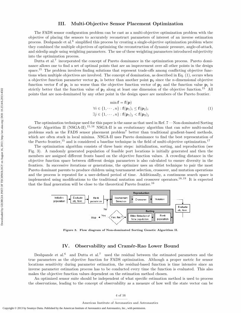
The optimization algorithm consists of three basic steps: initialization, sorting, and reproduction (seeFig. 3). A randomly generated population of feasible port locations is initially generated and then themembers are assigned different fronts based on the objective function values. A crowding distance in theobjective function space between different design parameters is also calculated to ensure diversity in thefrontiers. In successive iterations or generations, the optimizer uses an elitist technique to pair the mostPareto dominant parents to produce children using tournament selection, crossover, and mutation operationsand the process is repeated for a user-defined period of time. Additionally, a continuous search space isimplemented using modifications to the traditional mutation and crossover operators.18,19 It is expectedthat the final generation will be close to the theoretical Pareto frontier.16

Figure 3. Flow diagram of Non-dominated Sorting Genetic Algorithm II.

IV. Observability and Cramer-Rao Lower Bound

Deshpande et al.6 and Dutta et al.7 used the residual between the estimated parameters and thetrue parameters as the objective function for FADS optimization. Although a proper metric for sensorlocations sensitivity during parameter estimation, the residual-based function is time intensive since aninverse parameter estimation process has to be conducted every time the function is evaluated. This alsomakes the objective function values dependent on the estimation method chosen.

An optimized sensor suite should be independent of what specific estimation method is used to processthe observations, leading to the concept of observability as a measure of how well the state vector can be

4 of 16


Dow

nloa

ded

by G

EO

RG

IA I

NST

OF

TE

CH

NO

LO

GY

on

Aug

ust 1

6, 2

013

| http

://ar

c.ai

aa.o

rg |

DO

I: 1

0.25

14/6

.201

3-45

02


deduced from the outputs.20 Observability metrics can be found for linear, time-invariant systems using theobservability Gramian, but are hard to calculate for nonlinear, time-varying systems,21 such as the FADSsensors on a re-entry vehicle. The Cramer-Rao Lower Bound provides a useful substitute by defining thetheoretical lower bound of the expected uncertainty for an estimation process. CRLB is independent of theestimation method used and is defined as the inverse of the Fisher information matrix, which due to theGauss-Markov Theorem results in a simple inequality as shown in Eq. (2). In this expression P is the statecovariance matrix, H is the measurement sensitivity matrix, and R is the measurement noise covariance.

P ≥(HTR−1H

)−1(2)

If the measurement uncertainties are uncorrelated and can be represented by an identity matrix, theCRLB simplifies further to the expression in Eq. (3), which is only a function of the Jacobian of the mea-surement equation with respect to the state vector (or H). For FADS, the measurement equation is thepressure measured by a transducer and this value is a function of the transducer location, trajectory states,and atmospheric conditions.22

Plowest =(HTH

)−1(3)

V. Test Problem

The CRLB is calculated using the true state vector. These true states are provided here by the Programto Optimize Simulated Trajectories II (POST2),23 which was used to generate a nominal EDL trajectorythat is presented in Fig. 4. The trajectory is for a 4.5 m, 70-deg sphere-cone with the same geometryand specifications as MSL. This POST2-generated trajectory represents the truth data and the CRLB iscalculated with this truth data. MSL’s FADS objectives were defined while the dynamic pressure was 850Pa. or above; so in this investigation, the FADS sensor optimization is also limited to this time frame.

0 2 4 6−20

0

20

40

60

80

100

120

140

Velocity (km/s)

Alti

tude

(km

)

(a) Altitude vs. velocity

0 100 200 300 4000

5

10

15

20

25

30

Time (sec)

Mac

h nu

mbe

r

(b) Mach number

0 100 200 300 400

−80

−60

−40

−20

0

Time (sec)

Flig

ht p

ath

angl

e (d

eg.)

(c) Flight-path angle

0 50 100 150 200−21

−20

−19

−18

−17

−16

−15

−14

Time (sec)

Ang

le o

f atta

ck (

deg.

)

(d) Angle-of-attack

0 50 100 150 200−2

−1

0

1

2

Time (sec)

Sid

eslip

ang

le (

deg.

)

(e) Sideslip angle

0 100 200 300 4000

5

10

15

Time (sec)

Dyn

amic

pre

ssur

e (k

Pa)

Dyn. press.

850 Pa.

(f) Dynamic pressure

Figure 4. Simulated Mars EDL trajectory used for creating the dataset for sensor location optimization.

VI. CRLB Sensitivity to Trajectory

Dynamic pressure (q∞), angle of attack (α), and sideslip angle (β) are often the parameters of interest inFADS applications4,6, 12,13 and were also the quantities for which MSL’s science objectives were specified.3

These terms serve as the state vector here, which means that H and the CRLB-calculated P will be calculated

5 of 16


Dow

nloa

ded

by G

EO

RG

IA I

NST

OF

TE

CH

NO

LO

GY

on

Aug

ust 1

6, 2

013

| http

://ar

c.ai

aa.o

rg |

DO

I: 1

0.25

14/6

.201

3-45

02


with respect to these parameters. If only the diagonal of P is considered, then one gets uncorrelated varianceof each of the parameters of interest as seen in Eq. (4).

(HTH

)−1= Plowest =

σ2α

σ2β

σ2q∞

(4)

FADS optimization will locate a sensor configuration that minimizes the non-normalized, standard de-viation (σ) - square-root of the variance - for each parameter of interest over the length of the trajectory.Due to multiple parameters of interest, the function is multi-objective and the optimal configurations willbe part of Pareto frontiers. However, since the CRLB is calculated at a given trajectory condition, there willbe a CRLB for every trajectory point. The CRLB values throughout the trajectory need to be combinedinto one objective function vector that describes a metric of observability for a given FADS configuration.

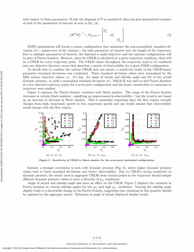
To decide how to combine the various CRLBs into one metric, a sensitivity study of the CRLB-based,parameter standard deviations was conducted. These standard deviation values were normalized by theMSL science objective values, i.e. 0.5 deg. for angle of attack and sideslip angle and 2% of the actualdynamic pressure, to yield a normalized standard deviation (σ). NSGA-II was used to find Pareto frontiersat a few selected trajectory points for a seven-port configuration and the fronts’ sensitivities to variations intrajectory were studied.

Figure 5 captures the Pareto frontier variation with Mach number. The range of the Pareto frontierdecreases at certain Mach numbers - signifying an improvement in observability - but the trend is not basedon an increase or decrease in Mach number. This is somewhat surprising since the flow regime actuallychanges from high, hypersonic speeds to low, supersonic speeds and one would assume that observabilitywould change with the flow regime.

0 0.2 0.4 0.60

0.05

0.1

0.15

0.2

0.25

0.3

0.35

σα

σ β

28.118.66.93.92.9

(a) σα vs. σβ

0 0.2 0.4 0.60

0.02

0.04

0.06

0.08

0.1

σα

σ q∞

28.118.66.93.92.9

(b) σα vs. σq∞

0 0.1 0.2 0.30

0.02

0.04

0.06

0.08

0.1

σβ

σ q∞

28.118.66.93.92.9

(c) σβ vs. σq∞

Figure 5. Sensitivity of CRLB to Mach number for the seven-port optimized configuration.

Instead, a stronger correlation is seen with dynamic pressure (Fig. 6), where higher dynamic pressurevalues lead to lower standard deviations and better observability. Due to CRLB’s strong sensitivity todynamic pressure, the metric used to aggregate CRLBs from various points in the trajectory should sampledifferent dynamic pressure values to have a diversity of q∞ conditions.

Angle of attack and sideslip angle also have an effect on the CRLB. Figure 7 displays the variation inPareto frontiers at various sideslip angles for low q∞ and high q∞ conditions. Varying the sideslip angleslightly leads to a discernible change in the Pareto frontier, suggesting that variations in this quantity shouldbe captured in the aggregate metric. Variations in angle of attack displayed similar trends.

6 of 16


Dow

nloa

ded

by G

EO

RG

IA I

NST

OF

TE

CH

NO

LO

GY

on

Aug

ust 1

6, 2

013

| http

://ar

c.ai

aa.o

rg |

DO

I: 1

0.25

14/6

.201

3-45

02


0 0.1 0.2 0.30

0.05

0.1

0.15

0.2

0.25

0.3

0.35

σα

σ β

0.91 kPa1.41 kPa6.85 kPa12.13 kPa15.80 kPa

(a) σα vs. σβ

0 0.1 0.2 0.30

0.01

0.02

0.03

0.04

0.05

0.06

0.07

σα

σ q∞


(b) σα vs. σq∞

0 0.1 0.2 0.30

0.01

0.02

0.03

0.04

0.05

0.06

0.07

σβ

σ q∞


(c) σβ vs. σq∞

Figure 6. Sensitivity of CRLB to dynamic pressure for the seven-port optimized configuration.

0 0.2 0.4 0.60

0.1

0.2

0.3

0.4

q∞=0.87 kPa

σ β

−0.58 deg.0.40 deg.

0.005 0.01 0.015 0.020

0.01

0.02

0.03

0.04

q∞=12.13 kPa

σα

σ β

−0.23 deg.0.24 deg.

(a) σα vs. σβ

0 0.2 0.4 0.60

0.05

0.1

q∞=0.87 kPa

σ q∞

−0.58 deg.0.40 deg.

0.005 0.01 0.015 0.020

1

2

3

4x 10

−3 q∞=12.13 kPa

σα

σ q∞

−0.23 deg.0.24 deg.

(b) σα vs. σq∞

0 0.1 0.2 0.30

0.05

0.1

q∞=0.87 kPa

σ q∞

−0.58 deg.0.40 deg.

0 0.01 0.02 0.030

1

2

3

4x 10

−3 q∞=12.13 kPa

σβ

σ q∞

−0.23 deg.0.24 deg.

(c) σβ vs. σq∞

Figure 7. Sensitivity of CRLB to sideslip angle for the seven-port optimized configuration.

VII. Objective Function Formulation

In this investigation, 20 sample locations from the test problem trajectory were selected for the aggregateobjective function. These discrete trajectory states are shown in Fig. 8 overlaid on the continuous trajectory.One can see that there has been equal distribution given to low and high dynamic pressure values and avariety of angle of attack and sideslip angles.

50 100 150 2000

5

10

15

Time (sec)

Dyn

amic

pre

ssur

e (k

Pa)

OriginalSampled

(a) Dynamic pressure

50 100 150 2000

5

10

15

20

25

30

Time (sec)

Mac

h nu

mbe

r

OriginalSampled

(b) Mach number

50 100 150 200−21

−20

−19

−18

−17

−16

−15

−14

Time (sec)

Ang

le o

f atta

ck (

deg)

OriginalSampled

(c) Angle of attack

50 100 150 200−0.8

−0.6

−0.4

−0.2

0

0.2

0.4

0.6

Time (sec)

Sid

eslip

ang

le (

deg)

OriginalSampled

(d) Sideslip angle

Figure 8. Sampled trajectory points for the aggregate objective function.

7 of 16


Dow

nloa

ded

by G

EO

RG

IA I

NST

OF

TE

CH

NO

LO

GY

on

Aug

ust 1

6, 2

013

| http

://ar

c.ai

aa.o

rg |

DO

I: 1

0.25

14/6

.201

3-45

02


Using these sampled points, the objective function f is defined in Eq. (5), while the optimization problemis defined in Eq. (6) where ¯ is the component-wise, arithmetic average of the objective functions. Theinequality constraint in Eq. (6) is used to maintain a minimum spacing between the n port locations (p),and this minimum distance dmin is chosen as 5 inches as it was done in Ref. 7.

f(p)i = [σα,i, σβ,i, σq∞,i]T ∀ i = {1, · · · , k} (5)

min f(p)

s.t. |pi − pj | ≤ dmin ∀ i, j ∈ {1, · · · , n}(6)

VIII. Optimization Results

A. Implementation and Computational Effort

The NSGA-II method is an evolutionary algorithm so finding the true Pareto frontier is not guaranteed.The CRLB-based optimization was conducted with a population of 128 candidate configurations over 500generations and this process was repeated 10 times. The final Pareto frontiers were found using the combinedresults. Experimentation showed that a population size of 128 provided a good distribution across the designspace to capture the near-optimal Pareto frontier and that 500 generations were enough to reach a stable setof non-dominated points. This process required in 640,000 function calls. These calls were made regardlessof the type of configuration being optimized, i.e. a three-port or a seven-port situation had the same numberof function calls. Additionally, the number of generations, population size, and number of repetitions wereselected with conservatism to ensure that the optimization converged. It is possible that similar results couldbe achieved with far fewer function calls.

On the other hand, a brute-force search, where each possible configuration was checked, would demand asignificantly larger number of function calls, especially as one increased the number of pressure transducersbeing optimized. This is described by Fig. 9 where the number of function calls using a Monte Carlo-likeprocess on a representative grid of possible transducer locations and the CRLB-based, NSGA-II optimizationprocess are compared. A smart culling process can reduce the grid size and the number of possible combi-nations to evaluate, but as shown in Fig. 9 even a coarser search grid size uses significantly more functioncalls compared to the NSGA-II optimization that uses a continuous search space.

−2 −1 0 1 2

−2

−1

0

1

2

Y (m)

Z (

m)

(a) Possible ports (with 1585 points ongrid)

4 6 810

0

1010

1020

1030

Number of ports

Num

ber

of fu

nctio

n ev

alua

tions

NSGA−II

100 pts.

792 pts.

1585 pts.

7921 pts.

(b) Comparison of number of functioncalls

Figure 9. Comparison of function evaluations between a Monte Carlo-based method with various number of points onthe grid and the CRLB-based optimization method.

In terms of computational speed, the CRLB-based objective function evaluation took around 10−3 susing a 3.4 GHz Intel i7 processor, with a slight increase in run time as the number of ports increased. Onthe other hand, Dutta et al.’s residual-based objective function took close to 25 s per run using the samehardware,7 underscoring the improvement in speed if the CRLB-based function is used. Deshpande et al.6

did not provide any computational data for comparison of their method.

8 of 16


Dow

nloa

ded

by G

EO

RG

IA I

NST

OF

TE

CH

NO

LO

GY

on

Aug

ust 1

6, 2

013

| http

://ar

c.ai

aa.o

rg |

DO

I: 1

0.25

14/6

.201

3-45

02


B. Multi-objective Optimization Pareto Frontiers

The results of the CRLB-based FADS optimization are summarized in Fig. 10, which shows different viewsof the Pareto surface formed by the three-objective optimization. Pareto frontiers for three-port throughnine-port configurations are shown. The two-port configuration did not provide a converged Pareto frontierin 500 generations and was excluded in this analysis.

0.005 0.01 0.015 0.020

0.01

0.02

0.03

0.04

0.05

0.06

σα

σ β

3−port4−port5−port6−port7−port8−port9−port

(a) σα vs. σβ

0 0.01 0.02 0.03 0.04 0.05 0.060

0.002

0.004

0.006

0.008

0.01

0.012

σα

σ q∞


(b) σα vs. σq∞

0 0.01 0.02 0.03 0.04 0.05 0.060

0.002

0.004

0.006

0.008

0.01

0.012

σβ

σ q∞


(c) σβ vs. σq∞

Figure 10. Pareto frontiers from multi-objective optimization for various port numbers.

Figure 10 shows that the Pareto frontiers come closer and closer to the origin as the number of portsincrease. This is not surprising, since empirical evidence suggests that increasing the number of portsimproves observability and leads to a lower objective function value. It also appears that the frontierscoalesce upon each other and not much is gained in observability after the six-port configuration. A six-port configuration thus appears to be the point of diminishing returns. The identification of the point ofdiminishing returns is investigated further later in this section.

Some representative configurations from the Pareto frontier are shown in Fig. 11. Although there is astructure to the port configurations, there was no constraint for symmetry and thus the optimized configu-rations are non-symmetrical. The representative configurations chosen in Fig. 11 are for either minimum σα,σβ , or σq∞ and the layouts exhibit these qualities. Dynamic pressure observability is achieved by placingports near the stagnation point, which for this trajectory was around y = 0 and z = -1 m. Angle of attackobservability is achieved by placing ports in the pitch plane on either side of the origin, while sideslip angleobservability is maintained in a similar way except in the yaw plane. Numerical effects of the optimiza-tion are apparent in Fig. 11(b), where intuition would suggest that all of the ports would have z = 0, andFig. 11(c), where all of ports don’t have y = 0. Due to numerical noise, the optimization may not capturethese nuances very well.

−2 −1 0 1 2

−2

−1

0

1

2

Y (m)

Z (

m)

(a) Min. σq∞ 3-port

−2 −1 0 1 2

−2

−1

0

1

2

Y (m)

Z (

m)

(b) Min. σβ 4-port

−2 −1 0 1 2

−2

−1

0

1

2

Y (m)

Z (

m)

(c) Min. σα 7-port

Figure 11. Port configurations from some representative points of the Pareto frontiers.

Although single objective optimal results are interesting to study, designers are more interested in configu-rations that can achieve good performance in all of the objective functions. Every point of the Pareto frontieris a non-dominated solution and hence it is hard to pick one point over another; however, one can define anequally-weighted compromise point which is closest to the ideal solution. The definition of this compromise

9 of 16


Dow

nloa

ded

by G

EO

RG

IA I

NST

OF

TE

CH

NO

LO

GY

on

Aug

ust 1

6, 2

013

| http

://ar

c.ai

aa.o

rg |

DO

I: 1

0.25

14/6

.201

3-45

02


point may differ due to the type of weighting applied; however, the simplest such compromise point wouldcome from a linear weighting scheme. Figure 12 explains the meaning of this linearized, equally-weightedcompromise point on a nominal Pareto frontier.

Figure 12. Definition of the linearized, equally-weighted compromise point of a Pareto frontier.

Using the linearized, equally-weighted compromise point as a benchmark of a good design, Fig. 13 showssome representative optimal configurations for various number of ports. Some broad design ideas can begleaned from these configurations. It appears that annular like layouts - where ports are laid out in rings -are more preferred using this benchmark than cruciform layouts that were seen in some past configurations(Fig. 2). Additionally, many of these ports are concentrated near a ring of radius 0.5 m, which is near thearea of a change in curvature as the aeroshell shape transitions from a spherical segment to the sharp cone.A change in curvature or geometry would make a port located in that region very sensitive to changes in thetrajectory. Finally, all of the configurations have a port or two located near the stagnation point, suggestingthat measuring pressure in this region improves observability of all of the parameters.

−2 −1 0 1 2

−2

−1

0

1

2

Y (m)

Z (

m)

(a) 3-port

−2 −1 0 1 2

−2

−1

0

1

2

Y (m)

Z (

m)

(b) 5-port

−2 −1 0 1 2

−2

−1

0

1

2

Y (m)

Z (

m)

(c) 7-port

−2 −1 0 1 2

−2

−1

0

1

2

Y (m)

Z (

m)

(d) 8-port

Figure 13. Port configurations of some of the linearized, equally-weighted compromise points of the Pareto frontiers.

Interestingly, some of the configurations shown could be simplified further. For example, the 7-portconfiguration in Fig. 13(c) shows two ports near z = −1. If these two ports are combined to create a 6-portconfiguration, the objective function values does not degrade significantly from the 7-port values. Thus,although numerical optimization can quickly narrow down the design space to a list of good designs, it stillleaves room for intuitive improvements by the designer.

The linearized, equally-weighted compromise point also allows one to visualize the point of diminishingreturns. The diminishing point is apparent in Fig. 14, where the objective function values of the represen-tative point of the Pareto frontier are plotted for different port configurations. If one is interested in onlydynamic pressure reconstruction, a 5-port configuration seems to suffice as the point of diminishing returns.The Pareto contours in Figs. 10(b) and 10(c) that contain dynamic pressure dependency also support thisassertion. However, when all of the parameters are considered together, one needs at least 6-ports to reachthe point of diminishing returns, since the marginal return point is not reached for angle of attack andsideslip angle until this port configuration as seen in Fig. 14 and the Pareto frontier in Fig. 10(a).

10 of 16


Dow

nloa

ded

by G

EO

RG

IA I

NST

OF

TE

CH

NO

LO

GY

on

Aug

ust 1

6, 2

013

| http

://ar

c.ai

aa.o

rg |

DO

I: 1

0.25

14/6

.201

3-45

02


3 4 5 6 7 8 90

0.002

0.004

0.006

0.008

0.01

Number of ports

σ α

(a) Angle of attack

3 4 5 6 7 8 90

1

2

3

4

5x 10

−3

Number of ports

σ β

(b) Sideslip angle

3 4 5 6 7 8 90

0.5

1

1.5x 10

−3

Number of ports

σ q∞

(c) Dynamic pressure

Figure 14. Identification of the point of diminishing return for non-symmetric configurations using objective values ofthe linearized, equally-weighted compromise points.

IX. Sensitivity to Pressure Models

The pressure model used to evaluate the objective function has a sensible effect on the optimizationresults. In Sec. VIII, a Computational Fluid Dynamics (CFD) derived pressure distribution was used inthe function evaluations. However, CFD results have some uncertainties associated with them. One canuse the classical Newtonian model to represent the pressure distribution, as was done by Deshpande et al.6

Figure 15 captures the effect of using various pressure distributions by showing the Pareto frontiers for a6-port configuration with the nominal CFD distribution, a CFD-based distribution perturbed randomly by5%, and a Newtonian distribution.

0 0.01 0.02 0.03 0.04

0.005

0.01

0.015

0.02

0.025

0.03

0.035

0.04

0.045

0.05

σα

σ β

NominalPerturbedNewton

(a) σα vs. σβ

0 0.01 0.02 0.03 0.04

1

2

3

4

5

6

7

8

9

x 10−3

σα

σ q∞


(b) σα vs. σq∞

0 0.01 0.02 0.03 0.04 0.05

1

2

3

4

5

6

7

8

9

x 10−3

σβ

σ q∞


(c) σβ vs. σq∞

Figure 15. Comparison of Pareto frontiers for the 6-port configurations using various pressure models.

One does not see a major difference between the results of the two CFD-based optimizations, but theNewtonian distribution’s Pareto frontier in the α-β slice appears less structured. Since the Newtoniandistribution is based on a smooth function 2 sin θ2 there are multiple port configurations that have similarobjective function values and that makes the objective function space multi-modal.

Similar conclusions can be drawn when looking at the configurations described by the Pareto frontiers.Figure 16 shows the minimum σα configurations for the 6-port case using different pressure models. Asexpected for a suite making angle of attack more observable, all three configurations have transducers thatare located on the pitch plane and have sets of ports that are on either side of the origin to increase thesensitivity to changes in the angle of attack. Due to the accumulation of ports in two locations, it seemsthat if one was only interested in angle of attack reconstruction a 2-port solution could suffice. In reality,designers are interested in reconstructing more than one parameter and hence would not be interested in anoptimal configuration for only one parameter.

The nominal and perturbed CFD-based configurations yield extremely similar results, while the New-tonian configuration is different. As the CFD-distribution is not as smooth as the Newtonian pressuredistribution, the objective function space is less multi-modal and the configurations shown in Figs. 16(a)and 16(b) represent samples from a basin of attraction. The Newtonian distribution-based objective space

11 of 16


Dow

nloa

ded

by G

EO

RG

IA I

NST

OF

TE

CH

NO

LO

GY

on

Aug

ust 1

6, 2

013

| http

://ar

c.ai

aa.o

rg |

DO

I: 1

0.25

14/6

.201

3-45

02


−2 −1 0 1 2

−2

−1

0

1

2

Y (m)

Z (

m)

(a) Nominal

−2 −1 0 1 2

−2

−1

0

1

2

Y (m)

Z (

m)

(b) Perturbed

−2 −1 0 1 2

−2

−1

0

1

2

Y (m)

Z (

m)

(c) Newtonian

Figure 16. Optimal σα 6-port configuration using various pressure models.

is more multi-modal and vastly different looking configurations are represented in the Pareto frontiers.This exercise underscores the need to use computational methods to optimize a FADS suite and to tailor

it for the proper conditions. Simply relying on engineering judgment and pressure distribution predictionsfrom one set of tools - the modus operandi of designing FADS configurations in the past - is not enough todesign a robust sensor suite. The variations caused by using different pressure distributions can be significant.

X. Sensitivity to Trajectory Perturbations

One of the main assertions of this comprehensive FADS placement optimization procedure is to makethe chosen configuration robust and optimal over the entire trajectory. The effect of trajectory variationsis clearly visible in Fig. 17 which shows the Pareto frontiers of a 6-port configurations using the nominaltrajectory defined in Sec. VII and another trajectory perturbed by 5% from the nominal. Even though theperturbation is small, the Pareto frontiers show a visible difference.

0 0.01 0.02 0.03 0.04 0.05

0.005

0.01

0.015

0.02

0.025

0.03

0.035

0.04

0.045

0.05

0.055

σα

σ β

NominalPerturbed

(a) σα vs. σβ

0.01 0.02 0.03 0.04 0.050

1

2

3

4

5

6

7x 10

−3

σα

σ q∞

NominalPerturbed

(b) σα vs. σq∞

0 0.01 0.02 0.03 0.04 0.05 0.060

1

2

3

4

5

6

7x 10

−3

σβ

σ q∞

NominalPerturbed

(c) σβ vs. σq∞

Figure 17. Comparison of Pareto frontiers for the 6-port configurations using various trajectories.

The effect of trajectory variation is also apparent in the optimized FADS configurations for minimumσq∞ shown in Fig. 18. As expected, the ports optimizing the reconstruction of dynamic pressure are centeredaround the stagnation point. However, the slight difference between the optimal σq∞ nominal (Fig. 18(a))and perturbed (Fig. 18(b)) trajectory leads to a different looking port configuration. On the other hand,Fig. 18(c) shows a very different looking configuration that does not have the best σq∞ value for either casebut is still robust to the two different trajectories. This emphasizes the effect of trajectory perturbation andwhy FADS optimization should be performed across the entire trajectory and not at a single point of thetrajectory. This way solutions that are robust to such perturbations can be found instead of optima basedon point designs.

12 of 16


Dow

nloa

ded

by G

EO

RG

IA I

NST

OF

TE

CH

NO

LO

GY

on

Aug

ust 1

6, 2

013

| http

://ar

c.ai

aa.o

rg |

DO

I: 1

0.25

14/6

.201

3-45

02


−2 −1 0 1 2

−2

−1

0

1

2

Y (m)

Z (

m)

(a) Nominal

−2 −1 0 1 2

−2

−1

0

1

2

Y (m)

Z (

m)

(b) Perturbed

−2 −1 0 1 2

−2

−1

0

1

2

Y (m)

Z (

m)

(c) Robust

Figure 18. Optimal σq∞ 6-port configuration using different trajectories.

XI. Optimization with Symmetry Constraints

Past FADS sensors have had symmetric configurations (Fig. 2) and the FADS optimization study con-ducted by Deshpande et al.6 explicitly set symmetry as a constraint. Due to the preference of symmetry inthese past configurations, the optimization was also conducted with a symmetric constraint to look at howthis affected the optimal configurations. The new objective function is shown in Eq. 7 and this optimizationwas repeated with various numbers of even-numbered pressure ports.

min f(p)

s.t. |pi − pj | ≤ dmin ∀ i, j ∈ {1, · · · , n}pi,y = −pj,y ∀ i ∈ {1, · · · , n/2} and j = i+ n/2

pi,z = pj,z

(7)

The Pareto frontiers of the design space are shown in Fig. 19. Once again, 2-port configurations wereexcluded due to their poor convergence in the optimization. The number of ports that serves as the point ofdiminishing returns may be determined using Fig. 20, which shows the objective function of the linearized,equally-weighted compromise points. For certain objectives, like sideslip angle, there seems to be littledifference in objective value by increasing the number of ports and the point of diminishing returns appearsto be at 4-port configurations. If one is interested in only sideslip angle reconstruction, a 4-port configurationcould suffice. But overall, considering all of the objectives at once, it appears that 6-port configurations arethe points of diminishing returns as the Pareto frontiers coalesce upon each other as the number of portsincrease and only marginal improvement in the uncertainty is gained by increasing the number of ports.

0 0.02 0.04 0.06 0.08 0.10

0.005

0.01

0.015

0.02

0.025

0.03

0.035

0.04

0.045

σα

σ β

4−port6−port8−port10−port

(a) σα vs. σβ

0 0.02 0.04 0.06 0.08 0.10

0.002

0.004

0.006

0.008

0.01

0.012

0.014

0.016

0.018

0.02

σα

σ q∞


(b) σα vs. σq∞

0 0.01 0.02 0.03 0.040

0.002

0.004

0.006

0.008

0.01

0.012

0.014

0.016

0.018

0.02

σβ

σ q∞


(c) σβ vs. σq∞

Figure 19. Pareto frontiers from multi-objective optimization for various port numbers with symmetry constraints.

The port configurations related to the linearized, equally-weighted compromise point of the Pareto fron-tiers are shown in Fig. 21.

There are some generalizing trends that can be observed when comparing the representative symmet-ric, linearized, equally-weighted compromise point configurations with their non-symmetric counterparts in

13 of 16


Dow

nloa

ded

by G

EO

RG

IA I

NST

OF

TE

CH

NO

LO

GY

on

Aug

ust 1

6, 2

013

| http

://ar

c.ai

aa.o

rg |

DO

I: 1

0.25

14/6

.201

3-45

02


4 6 8 100

0.002

0.004

0.006

0.008

0.01

Number of ports

σ α

(a) Angle of attack

4 6 8 100

1

2

3

4

5

6

7x 10

−3

Number of ports

σ β

(b) Sideslip angle

4 6 8 100

1

2

3

4

5x 10

−3

Number of ports

σ q∞

(c) Dynamic pressure

Figure 20. The point of diminishing return of symmetric configurations found using objective function values of thelinearized, equally-weighted compromise point.

−2 −1 0 1 2

−2

−1

0

1

2

Y (m)

Z (

m)

(a) 4-port

−2 −1 0 1 2

−2

−1

0

1

2

Y (m)

Z (

m)

(b) 6-port

−2 −1 0 1 2

−2

−1

0

1

2

Y (m)Z

(m

)

(c) 8-port

−2 −1 0 1 2

−2

−1

0

1

2

Y (m)

Z (

m)

(d) 10-port

Figure 21. Port configurations of the linearized, equally-weighted compromise points of the symmetric optimization’sPareto frontiers.

Fig. 13. Similar to the situation with the non-symmetric cases, the optimal configurations appear to beannular rather than cruciform shaped. The ring of ports are in the region where the aeroshell shape tran-sitions from a spherical segment to a cone. These design guides seem to reinforce lessons learned from thenon-symmetric optimization. However, upon comparing their respective objective function values, as shownin Table 1, the effect of the slight differences between the two optimizations are apparent. The table showsthat although the symmetric constraint leads to slight improvements in some objective function values overthe non-symmetric cases, there is always one objective function value where the symmetric case performsvery poorly compared to its non-symmetric counterpart. It can be inferred then that symmetric constraintsmay hinder the observability of the sensor suite in some fashion over the non-symmetric constrained results.

Table 1. Comparison between non-symmetric and symmetric configurations using the linearized, equally-weightedcompromise points.

Percent difference from

Ports non-symmetric values

%σ∗α %σ∗β %σ∗q∞

4 57.30 -14.92 11.37

6 -13.26 37.22 -5.31

8 -27.12 32.55 -11.95

XII. Optimizing for Low Dynamic Pressure and Wind Speed Reconstruction

The observability of angle of attack, sideslip angle, and dynamic pressure were optimized by the objectivefunction chosen in this study. However, wind speeds are also often important parameters of interest, and thereare techniques that leverage FADS measurements and on-board IMU data to estimate these quantities.24

Thus, the observability of wind speeds can also be a quantity that is added to the objective function.However, past studies have shown that the wind speed estimation is more a function of the IMU-based

14 of 16


Dow

nloa

ded

by G

EO

RG

IA I

NST

OF

TE

CH

NO

LO

GY

on

Aug

ust 1

6, 2

013

| http

://ar

c.ai

aa.o

rg |

DO

I: 1

0.25

14/6

.201

3-45

02


velocity reconstruction,2 so other changes to the objective function have to be also made to reflect thissituation.

Another potential modification is to capture the effect of the measurement or sensor uncertainty in theobjective function. Recall that for this objective function formulation the measurement noise covariance,R, was assumed to be an identity matrix. In actual sensors, the measurement uncertainty varies based onthe flight regime or the dynamic pressure value and this can be reflected by varying R with the trajectory.In fact, FADS transducers are usually classified as either high dynamic pressure or low dynamic pressuresensors and engineers often design a port configuration for only one of these situations. For example, theMEADS suite that flew on MSL was only optimally calibrated for dynamic pressures above 850 Pa. althoughthe transducers continued to take pressure measurements well below that limit. So one can optimize portconfigurations by including a varying R in the objective function and obtain results where one set of portsare optimized for high dynamic pressure regimes and another set is optimized for the low dynamic pressureregime.

XIII. Conclusions

Flush atmospheric data systems often serve as critical sensors of orientation angles and freestream con-ditions in atmospheric entry and flight dynamics applications. However, the design of most past flushatmospheric data system configurations was based on engineering judgment rather than a physics-basedmodel. Additionally, the few studies that looked into the optimization of flush atmospheric data systemseither did not consider the entire trajectory or had computationally expensive objective functions.

The current investigation uses the concept of observability to calculate objective functions that improvethe ability to estimate angle of attack, sideslip angle, and dynamic pressure. Specifically, the Cramer-Rao Lower Bound is used to define the lowest possible standard deviation of the parameters of interest.The effect of trajectory is considered in creating the objective function value and it is found that dynamicpressure plays the most important role in the value of the Cramer-Rao-based uncertainties. An evolutionaryoptimization technique based on Genetic Algorithms is used to conduct the multi-objective optimization andPareto frontiers are found for various port configurations. The optimization is conducted at first withoutany symmetrical constraints and then with symmetry enforced as a constraint. If one is interested in asingle objective optimization, such as angle of attack or dynamic pressure, a 4 or 5-port configuration maybe the point of diminishing returns depending on the parameter of interest. But when all parameters areconsidered, both symmetric and non-symmetric cases showed that a 6-port configuration is the point ofdiminishing return for the test problem which is based on the Mars Science Laboratory trajectory. Hence,adding an additional port after the 6th port has minimal gain.

The port configurations from some representative Pareto frontier points suggest design trends for improv-ing observability. For instance, putting ports in annular fashion especially in the zone where a sphere-conetransitions from the spherical segment to the conical frustum seems to improve observability in all parametersof interest. Moreover, putting one or two ports near the stagnation point improves estimation of dynamicpressure greatly and this improvement also benefits other parameters of interest. The sensitivities of theoptimization to pressure models and trajectory perturbations were also considered and underscored the needof flush atmospheric data system designs that are robust to a variety of conditions.

This study demonstrated a low computational cost, multi-objective optimization method that can be usedto address the gap of physics-based flush atmospheric data system design methods. This method quicklyallows a designer to determine design trends for robust configurations that maximize the observability ofparameters of interest and the methods are easily amenable to include other parameters of interests.

Acknowledgments

A NASA Research Announcement (NRA) award (No. NNX12AF94A) has supported the tool develop-ment effort. The authors want to thank Chris Karlgaard of Analytical Mechanics Associates, Inc. and MarkSchoenenberger and Scott Striepe of NASA Langley Research Center for their advice and help in acquiringthe simulated datasets and other related tools.

15 of 16


Dow

nloa

ded

by G

EO

RG

IA I

NST

OF

TE

CH

NO

LO

GY

on

Aug

ust 1

6, 2

013

| http

://ar

c.ai

aa.o

rg |

DO

I: 1

0.25

14/6

.201

3-45

02


References

1Dutta, S., Braun, R., Russell, R., Striepe, S., and Clark, I., “Comparison of Statistical Estimation Techniques for Mars En-try, Descent, and Landing Reconstruction,” Journal of Spacecraft and Rockets, accessed May, 24, 2013. doi: 10.2514/1.A32459.

2Karlgaard, C. D., Beck, R. E., Keefe, S. A., Siemers, P. M., White, B. A., Engelund, W. C., and Munk, M. M., “MarsEntry Atmospheric Data System Modeling and Algorithm Development,” AIAA 2009-3916, AIAA Thermophysics Conference,San Antonio, TX, 2009.

3Gazarik, M. J., Wright, M. J., Little, A., Cheatwood, F. M., Herath, J. A., Munk, M. M., Novak, F. J., and Martinez,E. R., “Overview of the MEDLI Project,” IEEEAC 1510, IEEE Aerospace Conference, Big Sky, MT, 2008.

4Siemers, P. M. and Larson, T. J., “Space Shuttle Orbiter and Aerodynamic Testing,” Journal of Spacecraft , Vol. 16,No. 4, 1979, pp. 223–231.

5Cobleight, B., Whitmore, S., Haering, J. E., Borrer, J., and Roback, V., “Flush Airdata Sensing System CalibrationProcedures and Results for Blunt Forebodies,” Tech. rep., NASA TP-1999-209012, 1999.

6Deshpande, S., Kumar, R., Seywald, H., and Siemers, P., “Air data system optimization using a genetic algorithm,”AIAA 1992-4466, AIAA Guidance, Navigation, and Control Conference, Hilton Head, SC, 1992.

7Dutta, S., Braun, R., and Karlgaard, C., “Atmospheric Data System Sensor Placement Optimization for Mars Entry,Descent, and Landing,” Journal of Spacecraft and Rockets, accessed July 12, 2013. doi: 10.2514/1.A32515.

8Bar-Shalom, Y., Li, X., and Kirubarajan, T., Estimation with Applications to Tracking and Navigation, John Wiley &Sons, Inc., New York, NY, 2001.

9Nehoria, A. and Hawkes, M., “Performance Bounds for Estimating Vector Systems,” IEEE Transactions in SignalProcessing, Vol. 48, No. 6, 2000, pp. 1737–1749.

10Ingoldby, R., Michel, F., Flaherty, T., Doty, M., Preston, B., Villyard, K., and Steele, R., “Entry Data Analysis forViking Landers 1 and 2,” Tech. rep., NASA CR 159388, 1976.

11Blanchard, R. C. and Walberg, G. D., “Determination of the Hypersonic-Continnum/Rarefied-Flow Drag Coefficient ofthe Viking Lander Capsule 1 Aeroshell from Flight Data,” Tech. rep., NASA TM 1793, 1980.

12Pruett, C. D., Wolf, H., Heck, M. L., and Siemers, P. M., “Innovative Air Data System for the Space Shuttle Orbiter,”Journal of Spacecraft and Rockets, Vol. 20, No. 1, 1983, pp. 61–69.

13Whitmore, S., Moes, T., and Larson, T., “High Angle-of-Attack Flush Airdata Sensing System,” Journal of Aircraft ,Vol. 29, No. 5, 1992, pp. 915–919.

14Edquist, K. T., Dyakonov, A. A., Wright, M. J., and Tang, C. Y., “Aerothermodynamic Design of the Mars ScienceLaboratory Heatshield,” AIAA 2009-4075, AIAA Thermophysics Conference, San Antonio, TX, 2009.

15Deb, K., Multi-Objective Optimization using Evolutionary Algorithms, John Wiley & Sons, Ltd., 2001.16Deb, K., Pratap, A., Agarwal, S., and Meyarivan, T., “A Fast and Elitist Multiobjective Genetic Algorithm: NSGA-II,”

IEEE Transactions on Evolutionary Computation, Vol. 6, No. 2, 2002, pp. 182–197.17Reyes-Sierra, M. and Coello Coello, C. A., “Multi-Objective Particle Swarm Optimizers: A Survey of the State-of-the-

Art,” International Journal of Computational Intelligence Research, Vol. 2, No. 3, 2006, pp. 287–308.18Deb, K. and Agarwal, R., “Simulated Binary Crossover for Continuous Search Space,” Complex Systems, Vol. 9, 1995,

pp. 115–148.19Beyer, H.-G. and Deb, K., “On Self-Adaptive Features in Real-Parameter Evolutionary Algorithms,” IEEE Transactions

in Evolutionary Computation, Vol. 5, 2001, pp. 250–270.20Tapley, B. D., Schutz, B., and Born, G., Statistical Orbit Determination, Elsevier Academic Press, Burlington, MA,

2004.21Crassidis, J. and Junkins, J., Optimal Estimation of Dynamic Systems, Chapman & Hall/CRC, 2004.22Dutta, S. and Braun, R., “Mars Entry, Descent, and Landing Trajectory and Atmosphere Reconstruction,” AIAA 2010-

1210, AIAA Aerospace Sciences Meeting, Orlando, FL, 2010.23Striepe, S., Powell, R., Desai, P., Queen, E., Brauer, G., Cornick, D., Olson, D., and Peterson, F., Program To Optimize

Simulated Trajectories (POST II), Vol. II: Utilization Manual, Version 1.1.6.G, 2004.24Kelly, G. M., Findlay, J. T., and Compton, H. R., “Shuttle Subsonic Horizontal Wind Estimation,” Journal of Spacecraft ,

Vol. 20, No. 4, 1983, pp. 390–397.

16 of 16


Dow

nloa

ded

by G

EO

RG

IA I

NST

OF

TE

CH

NO

LO

GY

on

Aug

ust 1

6, 2

013

| http

://ar

c.ai

aa.o

rg |

DO

I: 1

0.25

14/6

.201

3-45

02


cramer-rao lower bound optimization of flush atmospheric ... · cram er-rao lower bound...

Documents