Electronic copy available at: http://ssrn.com/abstract=1262934

Crash-Neutral Currency Carry Trades

Jakub W. Jurek∗

Abstract

Currency carry trades exploiting violations of uncovered interest rate parity in G10 currencieshave historically delivered significant excess returns with annualized Sharpe ratios nearly twicethat of the U.S. equity market (1990-2008). Using data on foreign exchange options, this paperinvestigates whether these returns represent compensation for exposure to currency crashes. Aftereliminating net dollar exposure and hedging crash risk, excess returns to crash-neutral currencycarry trades are statistically indistinguishable from zero; returns to non-dollar-neutral portfoliosremain positive, but are only weakly significant. The choice of option maturity has a significantimpact on the realized excess returns, with quarterly hedging producing annualized returns thatare 1-2% higher than those obtained from monthly hedging.

First draft: October 2007

This draft: April 2009

∗Jurek: Princeton University, Bendheim Center for Finance, e-mail: jjurek@princeton.edu. I thank John Campbell,Itamar Drechsler, Steve Edelstein, John Galanek, John Heaton, Mark Mueller, Monika Piazzesi, Erik Stafford, AdrienVerdelhan, and seminar participants at Duke University, Yale University, the Fall 2008 NBER Asset Pricing Meeting,the 2008 Princeton-Cambridge Conference, the 2008 Princeton Implied Volatility Conference, the 2008 Conference onFinancial Markets, International Capital Flows and Exchange Rates (European University Institute), the 2009 Oxford-Princeton Workshop on Financial Mathematics and Stochastic Analysis, the Society for Quantitative Analysts andthe Harvard Finance Lunch (Fall 2007) for providing valuable comments. I am especially grateful to J.P. Morgan forproviding the FX option data.

Electronic copy available at: http://ssrn.com/abstract=1262934

Uncovered interest parity predicts that high interest rate currencies should depreciate relativeto low interest rate currencies, such that investors would be indifferent between holding the two.Empirically, not only do high interest rate currencies not depreciate relative to their low interestrate counterparts, they tend to appreciate. This finding, often referred to as the forward premiumanomaly, is one of the most prominent features of exchange rate data. Historically, the currencycarry trade – a strategy designed to exploit this anomaly – has delivered significant excess returnswith annualized Sharpe ratios nearly twice that of the U.S. equity market (Figure 1). Using data onforeign exchange options, this paper investigates whether these excess returns reflect compensationfor exposure to the risk of large devaluations (crashes) in currencies with high interest rates. I showthat after hedging crash risk, returns on portfolios of currency carry trades that are constructedto be dollar-neutral, are statistically indistinguishable from zero (1999-2008). Returns on portfoliosthat are not constrained to be dollar-neutral are only weakly significant and depend on the choiceof portfolio weights (equal- vs. spread-weighted). Finally, I examine the performance of the crashhedge during the credit crisis of 2008, and find significant improvements from using quarterly, ratherthan monthly, hedging.

The currency carry trade exploits the forward premium anomaly by borrowing funds in currencieswith low interest rates and lending them in currencies with high interest rates. This strategy capturesthe interest rate differential (carry) between the two currencies, but leaves the investor exposed tofluctuations in the exchange rate between the high interest rate currency and the low interest ratecurrency. Historically, since high interest rate currencies have tended to appreciate relative to theirlow interest rate counterparts, the currency exposure has actually turned out to be an additionalsource of return. As a result, currency carry trades have been characterized by an extremely attractiverisk-return tradeoff. For example, a simple strategy which equal-weighted nine individual carry tradesimplemented in currency pairs involving the U.S. dollar and one of the remaining G10 currenciesearned an annualized excess return of 4.42% with an annualized volatility of 5.05% (Sharpe ratio =0.88) over the period from January 1990 to December 2007.1 In the latter part of the sample (1999-2007), simple equal- and spread-weighted portfolios of carry trades delivered even higher Sharperatios of 1.06 and 1.35, respectively. To illustrate this, Figure 1 plots the total return indices forthe carry strategy vis a vis the total return indices for the three Fama-French risk factors andthe momentum portfolio. As can be readily seen from the plot, the returns to the carry strategydominate the returns to each of the alternatives when the strategies are scaled to have the same expost volatility. However, the currency carry trade is also exposed to the risk of significant declines,as evidenced by the 20% loss sustained in 2008, driving down the full sample Sharpe ratio to 0.57.

The returns to currency carry trades are characterized by two main features. First, the volatilityof the strategy is low and stands at roughly one half the volatility of any given X/USD exchangerate, suggesting that exchange rate innovations are largely uncorrelated in the cross-section. Second,

1The set of G10 currencies consists of: Australian dollar (AUD), Canadian dollar (CAD), Swiss franc (CHF), Euro(EUR), British pound (GBP), Japanese yen (JPY), Norwegian krone (NOK), New Zealand dollar (NZD), Swedishkrona (SEK), and the U.S. dollar (USD).

1

Electronic copy available at: http://ssrn.com/abstract=1262934

although the low volatility allows the total return index to have an extremely smooth upwardsprogression, the strategy is punctuated with infrequent, but severe, losses. The skewness of themonthly returns to the equal-weighted carry strategy over the period from January 1990 to December2008 is negative (-1.62) and its magnitude is nearly twice as large as the skewness of excess returnson the U.S. equity market or the momentum portfolio.2 The very high realized Sharpe ratio of thecarry trade and the prominence of negative skewness suggests that the excess returns earned bycurrency carry trade strategies may represent compensation for exposure to rare, but severe, crashesin currencies with relatively higher interest rates.3 This hypothesis parallels the claims of Barro(2006), Martin (2008) and Weitzman (2007), who argue that crash risk premia play an importantrole in reconciling estimates of the equity risk premium, and the findings of high volatility and crashrisk premia in equity option markets documented by Coval and Shumway (2001), Pan (2002), Bakshiand Kapadia (2003), and Driessen and Maenhout (2006) among others. Of course, the estimatedhistorical mean returns to the currency carry trade may suffer from an upward bias relative to theirpopulation counterparts, if the frequency and/or magnitude of crashes in the sample was unusuallylow (Rietz (1988)).

This paper contributes to the literature by investigating whether crash risk premia can accountfor the empirically observed violations of uncovered interest parity. Under the crash risk hypothesis,excess returns to currencies with relatively higher interest rates represent compensation for exposureto the risk of rapid, large devaluations. In the ensuing analysis, I define crashes as exchange rateshocks that exceed some pre-specified threshold or a multiple of the option-implied volatility. Onceexposure to crash risk is hedged, excess returns to currency carry trades are predicted to decline,or be eliminated altogether, if the exposure to currency crashes is the sole risk factor for whichinvestors demand compensation. To investigate the crash risk hypothesis, I adopt two lenses. First,I investigate the time-series properties of the risk-neutral moments (variance, skewness and kurtosis)extracted from foreign exchange options. Since the distributions of currency returns embedded inoption prices are forward-looking, they provide a convenient approach for assessing the market’sex ante perceptions regarding the likelihood of crashes, as well as, the cost of insuring against suchevents. Contrary to the predication of the crash risk hypothesis, I find that risk-neutral skewness doesnot forecast excess currency returns.4 Nonetheless, the dynamics of risk-neutral skewness exhibitvery interesting behavior. In particular, I show that option-implied and realized skewness respondin opposite directions to lagged currency returns, such that the option-implied skewness forecasts

2Brunnermeier, Nagel and Pedersen (2008) argue that realized skewness is related to rapid unwinds of carry tradepositions, precipitated by shocks to funding liquidity. Plantin and Shin (2008) provide a game-theoretic motivation ofhow strategic complementarities, which lead to crowding in carry trades, can generate currency crashes.

3Currency carry trade returns generally appear to be unrelated to risk factors proposed by traditional asset pricingmodels (Burnside, et. al (2006)), although Lustig and Verdelhan (2007a, 2007b) dispute these findings and argue infavor of a consumption risk factor. Brunnermeier, Gollier, and Parker (2007) argue that high returns of negativelyskewed assets may be a general phenomenon.

4Bates (1996) arrives at a similar conclusion for dollar/yen and dollar/mark exchange rates during in the 1984-1992 sample. Unlike his paper, which relies on a calibrated jump-diffusion model, I use model-free estimates of therisk-neutral moments. Farhi, et al. (2009) propose a theoretical decomposition similar in spirit to Bates (1996), butderived in a stochastic discount factor (SDF) framework, in which the marginal utilities in two countries are driven bya combination of Gaussian shocks and Poisson jumps.

2

future realized skewness negatively. These facts suggest that insurance against crashes is actuallycheapest precisely when the risk of crashes is largest.

Second, in order to estimate currency crash risk premia, I investigate the returns to carry tradesin which the risk of currency crashes has been completely eliminated through hedging in the foreignexchange option market.5 In the 1999-2007 subsample, I find that portfolio excess returns remainstatistically significant only when the portfolios are not constrained to be dollar neutral, with equal-and spread-weighted portfolios of crash-neutral currency carry trades hedged using out-of-the-money(10δ) options delivering excess returns of 3.85% (t-stat: 2.76) and 6.55% (t-stat: 3.59), respectively.The mean excess returns to crash-neutral carry trades are statistically significantly lower than fortheir unhedged counterparts, with the difference in returns indicating that up to 35% of the return onthe unhedged trade is attributable to a crash risk premium. Driving the point estimates of the meanexcess returns to zero, would have required implied volatilities for out-of-the-money options to benearly four times their actual observed values, requiring a massive mispricing in the foreign exchangeoption market. More strikingly, returns on portfolios of crash-neutral currency carry trades that havebeen constrained to also maintain a zero net dollar exposure are not statistically, distinguishable fromzero. Moreover, once the sample is extended to include 2008, even the returns on the non-dollar-neutral portfolios are either borderline significant at conventional levels or indistinguishable fromzero.

Finally, I use the credit crisis of 2008 – a period during which the carry trade loses nearly 20% overa period of three months – as an event study for evaluating the performance of the proposed crashhedging strategies. Interestingly, the carry trade experiences a gradual sequence of adverse moves,rather than a single extreme jump, as typically postulated by models of rare disasters. If optionmarkets fail to appreciate this feature ex ante, rolling short-dated crash protection (e.g. one-monthoptions) is likely to be more expensive than purchasing longer dated options. I find that this isindeed the case, and that returns to carry trades hedged using three-month options are 1-2% higherper year than the returns to strategies employing one-month options. I conclude with a comparisonof hedging strategies based on hedging in fixed moneyness space, as opposed to fixed option deltaspace. Hedging positions in fixed delta space has the potentially unattractive feature that tradesare exposed to progressively larger losses as volatility rises, since fixing delta intuitively amounts tofixing the probability of having the crash-protection expire in-the-money. However, I find that thisfeature turns out to play a quantitatively minor role even during the crisis of 2008, when comparedwith hedging at a fixed distance to the prevailing forward prices. While fixing the option moneynessensures that the maximum percentage loss is constant over time, it also requires buying much morecostly (i.e. closer to at-the-money) protection throughout the crisis period.

5Bhansali (2007) examines the relation between option-implied volatilities and interest rate differentials, and pro-poses carry trade strategies involving at-the-money options. In related work, Burnside, et al. (2008) use at-the-moneyoptions to evaluate the impact if peso problem on estimates of carry trade returns.

3

1 The Currency Carry Trade

The expectations hypothesis of exchange rates, also known as uncovered interest parity (UIP),postulates that investors should be indifferent between holding riskless deposits denominated invarious currencies. Equivalently, high interest rate currencies are expected to depreciate relative tolow interest rate currencies, such that the currency return exactly offsets the interest rate differential.If this were the case, the forward exchange rate for a currency – the rate at which one can contractto buy/sell a foreign currency at a future date – would provide an unbiased estimate of the futureexchange rate. This relationship turns out to be frequently violated in the data leading to a forwardpremium anomaly, whereby high interest rate currencies actually tend to appreciate, rather thandepreciate, against their low interest rate counterparts.

The currency carry trade is designed to exploit this anomaly and involves borrowing funds ina currency with a low interest rate and lending them in a currency with a high interest rate. Atsome future date the proceeds from lending in the high-interest rate currency are converted backinto the funding currency, and used to cover the low-interest rate loan. The balance of the proceedsconstitutes the profit/loss from the carry trade, and can be thought of as a combination of the interestrate differential (carry) and the realized currency return. However, since the carry is known ex ante,and is riskless in the absence of counterparty risk, the sole source of risk in the carry trade stems fromuncertainty regarding future exchange rates. Principally, the carry trade exposes the arbitrageur torapid depreciations (crashes) of the currency which he is long vis a vis the funding currency. Thenext section documents the violations of UIP in the data and characterizes the historical returns tothe currency carry trade implemented in the set of G10 currencies.

1.1 Uncovered Interest Parity

Let the price of the foreign currency in terms of the domestic currency – taken to be the U.S.dollar – be St, such that an increase (decrease) in St corresponds to an appreciation (depreciation)of the foreign currency relative to the dollar. The forward rate, Ft,τ , which is the time t price forone unit of foreign currency to be delivered τ periods later, is determined through no arbitrage andsatisfies:

Ft,τ = St · exp ((rd,t − rf,t) · τ) (1)

where rf,t and rd,t are the time t foreign and domestic interest rates for τ -period loans. Thisrelationship is known as covered interest parity and is essentially never violated in the data.6 Whenthe foreign interest rate, rf,t, exceeds the domestic interest rate, rd,t, St is above Ft,τ and the foreigncurrency is said to trade at a premium to its forward. Conversely, when rd,t exceeds rf,t, the foreigncurrency trades at a discount (Ft,τ > St). Under UIP, the forward rate provides an unbiased estimate

6Empirical tests validating covered interest rate parity date back to Frenkel and Levich (1975); for a more recentassessment see Burnside, et al. (2006).

4

of the future spot exchange rate, a condition which is stated either in levels or logs,

Ft,τ = Et [St+τ ] or ft,τ = Et [st+τ ] (2)

If true, investors should be indifferent between buying the foreign currency at time t in the forwardmarket and converting their domestic currency to the foreign currency, investing in the foreign risklessbond and re-converting their investment proceeds back to the domestic currency at the future date.Empirical work, starting with Hansen and Hodrick (1980) and Fama (1984), tests UIP by regressingcurrency returns on the forward premium, defined as the difference between the prevailing forwardand spot prices.7 When expressed in logs the regression test takes on the following form,

st+1 − st = a0 + a1 · (ft − st) + εt+1 H0 : a0 = 0, a1 = 1 (3)

The null hypothesis under UIP is that the currency return is, in expectation, equal to the forwardpremium, which is given by the interest rate differential, (rd,t − rf,t) · τ . Although the empiricalprediction of this theory only holds in the absence of currency risk premia, it constitutes a usefulbenchmark for examining the data.

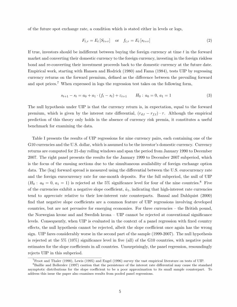
Table I presents the results of UIP regressions for nine currency pairs, each containing one of theG10 currencies and the U.S. dollar, which is assumed to be the investor’s domestic currency. Currencyreturns are computed for 21-day rolling windows and span the period from January 1990 to December2007. The right panel presents the results for the January 1999 to December 2007 subperiod, whichis the focus of the ensuing sections due to the simultaneous availability of foreign exchange optiondata. The (log) forward spread is measured using the differential between the U.S. eurocurrency rateand the foreign eurocurrency rate for one-month deposits. For the full subperiod, the null of UIP(H0 : a0 = 0, a1 = 1) is rejected at the 5% significance level for four of the nine countries.8 Fiveof the currencies exhibit a negative slope coefficient, a1, indicating that high-interest rate currenciestend to appreciate relative to their low-interest rate counterparts. Bansal and Dahlquist (2000)find that negative slope coefficients are a common feature of UIP regressions involving developedcountries, but are not pervasive for emerging economies. For three currencies – the British pound,the Norwegian krone and and Swedish krona – UIP cannot be rejected at conventional significancelevels. Consequently, when UIP is evaluated in the context of a panel regression with fixed countryeffects, the null hypothesis cannot be rejected, albeit the slope coefficient once again has the wrongsign. UIP fares considerably worse in the second part of the sample (1999-2007). The null hypothesisis rejected at the 5% (10%) significance level in five (all) of the G10 countries, with negative pointestimates for the slope coefficients in all countries. Unsurprisingly, the panel regression, resoundinglyrejects UIP in this subperiod.

7Froot and Thaler (1990), Lewis (1995) and Engel (1996) survey the vast empirical literature on tests of UIP.8Baillie and Bollerslev (1997) caution that the persistence of the interest rate differential may cause the standard

asymptotic distributions for the slope coefficient to be a poor approximation to its small sample counterpart. Toaddress this issue the paper also examines results from pooled panel regressions.

5

Cross-sectional regressions also consistently indicate that the further a currency’s lending rate isabove (below) the U.S. lending rate, the greater the anticipated appreciation (depreciation). Unlikein the time series regressions, in which the adjusted R2 of the forecasting regression is rarely above1%, the cross-sectional R2 is an order of magnitude higher. This suggests that although a tradeaimed at exploiting violations of UIP in a single currency may experience quite variable performanceover time, a portfolio trade exploiting the entire cross section of currency pairs is likely to be quitelucrative. Moreover, a portfolio of carry trades in which the weights of the individual currencies areset in proportion to the interest rate differential, or spread, is predicted to outperform an equal-weighted strategy.

Although the amount of predictability in the foreign exchange rate return at the one-month horizonis generally small, as evidenced by the low adjusted R2 values, the regressions indicate that investorscan earn excess returns by borrowing funds in the relatively low interest rate currency and lendingthem in the currency with the relatively high interest rate. This strategy, known as the currencycarry trade, in reference to the interest rate differential (carry) it earns, has historically been one ofthe most popular foreign exchange strategies. The next sections describe the carry trade strategy indetail and examine its historical performance to assess the economic significance of deviations fromUIP.

1.2 Exploiting deviations from UIP

In the standard carry trade an investor borrows money in a currency with a low interest rateand invests the proceeds in a currency with a high interest rate. To illustrate the payoff to thisstrategy consider an investor aiming to exploit the τ -month interest rate differential between thedomestic currency, bearing a low interest rate, and a foreign currency, bearing a high interest rate.The investor begins by borrowing St dollars at a rate of rd,t for a period of τ months in order tofinance the purchase of one unit of the foreign currency. After converting the funds to the foreigncurrency he lends them out for a period of τ months at the then prevailing foreign interest raterf,t. When the domestic currency is the relatively high interest rate currency, the investor employsa symmetric strategy and shorts one unit of the foreign currency. At time t + τ the payoff to thestrategy is given by:

CT t+1 =

{rf,t > rd,t : exp (rf,t · τ) · St+τ − exp (rd,t · τ) · Strd,t > rf,t : exp (rd,t · τ) · St − exp (rf,t · τ) · St+τ

(4)

If uncovered interest parity (UIP) held, the expected payoff to the carry trade would be zero, sinceSt+τ = Ft,τ , and the change in the exchange rate would exactly offset the interest differential (carry).However, in the presence of the empirically observed violations of UIP, the expected excess returnto the currency carry trade is positive. The corresponding carry trade return can be obtained bystandardizing the payoff by the funding capital – in this case given by the value of one unit of foreign

6

currency at initiation, St – to obtain:

RCTt+1 =

rf,t > rd,t : exp (rf,t · τ) ·(St+τSt

)− exp (rd,t · τ)

rd,t > rf,t : exp (rd,t · τ)− exp (rf,t · τ) ·(St+τSt

) (5)

Whenever rd,t < rf,t, the carry trader is long exposure to the foreign currency, and loses moneyif the foreign currency depreciates relative to the dollar by more than the interest rate differential.Symmetrically, when rf,t < rd,t, the carry trade investor borrows in the foreign currency and is shortexposure, and thus stands to earn a negative excess return if the foreign currency appreciates. Putdifferently, if exchange rates were defined as the price of the high interest rate currency in terms ofthe low interest rate currency, carry traders stand to earn a negative return in the event of a rapiddepreciation, or crash, of the high interest rate currency.

1.3 Historical performance

The historical performance of the currency carry trade is summarized in Tables IIa (1990-2007)and IIb (1999-2007). The strategy is implemented at a monthly frequency in nine pairs involvingone of the G10 currencies and the U.S. dollar, with positions established at the end of month t− 1and held until the end of month t. Within each pair, to determine which currency will be the long(short) leg of the trade I compare the one-month Eurocurrency rates prevailing at the end of montht− 1. Finally, since exchange rates are expressed in terms of units of domestic currency (U.S. dollar)per unit of foreign currency, the excess returns computed from (5) are interpretable as U.S. dollarreturns.

Over the full sample period the carry trade delivers positive excess returns in all nine currencypairs. For three of the individual currency pairs the excess returns are statistically different fromzero at the 5% significance level. The annualized Sharpe ratios vary from 0.14 (CHF/USD pair)to 0.75 (SEK/USD pair). Notably, however, the carry trade returns exhibit pronounced departuresfrom normality, with significant negative skewness and excess kurtosis. The minimum and maximummonthly returns are large in magnitude and represent roughly three standard deviation moves, whencompared with the the historically realized monthly volatility. These features are broadly represen-tative of the the carry trade and parallel the results reported in the existing literature (e.g. Burnside,et al. (2006), Brunnermeier, Nagel and Pedersen (2008)).

Panel B of Tables IIa and IIb presents the analogous summary statistics for portfolios of theindividual currency carry trades.9 Portfolios weighting the individual carry trades equally (EQL),or by the absolute interest rate spread at initiation (SPR), deliver positive and statistically significantreturns with annualized Sharpe ratios close to (1990-2007) or above (1999-2007) one. Of the total

9Carry trades constructed for investors whose domestic currency is one of the other nine G10 currencies have featuresthat are qualitatively comparable to those presented in Tables IIa and IIb. Results are available from the author byrequest.

7

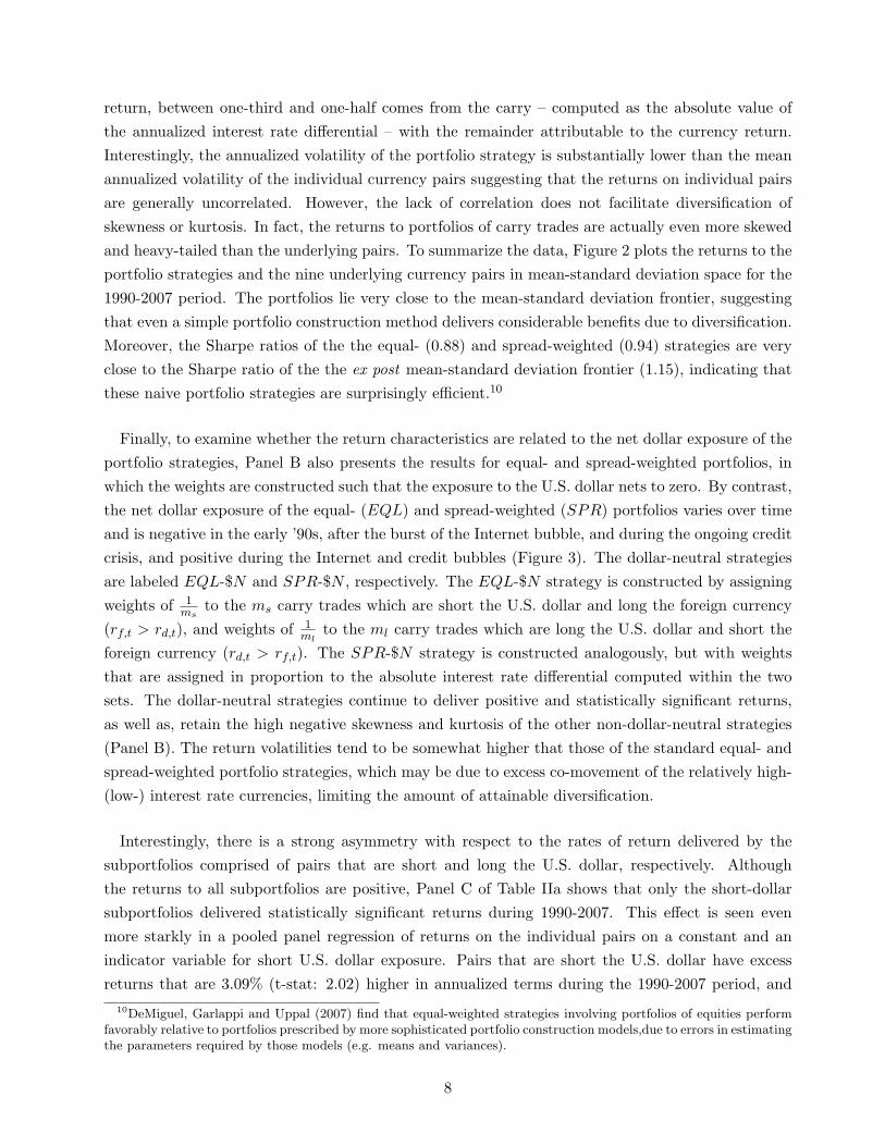
return, between one-third and one-half comes from the carry – computed as the absolute value ofthe annualized interest rate differential – with the remainder attributable to the currency return.Interestingly, the annualized volatility of the portfolio strategy is substantially lower than the meanannualized volatility of the individual currency pairs suggesting that the returns on individual pairsare generally uncorrelated. However, the lack of correlation does not facilitate diversification ofskewness or kurtosis. In fact, the returns to portfolios of carry trades are actually even more skewedand heavy-tailed than the underlying pairs. To summarize the data, Figure 2 plots the returns to theportfolio strategies and the nine underlying currency pairs in mean-standard deviation space for the1990-2007 period. The portfolios lie very close to the mean-standard deviation frontier, suggestingthat even a simple portfolio construction method delivers considerable benefits due to diversification.Moreover, the Sharpe ratios of the the equal- (0.88) and spread-weighted (0.94) strategies are veryclose to the Sharpe ratio of the the ex post mean-standard deviation frontier (1.15), indicating thatthese naive portfolio strategies are surprisingly efficient.10

Finally, to examine whether the return characteristics are related to the net dollar exposure of theportfolio strategies, Panel B also presents the results for equal- and spread-weighted portfolios, inwhich the weights are constructed such that the exposure to the U.S. dollar nets to zero. By contrast,the net dollar exposure of the equal- (EQL) and spread-weighted (SPR) portfolios varies over timeand is negative in the early ’90s, after the burst of the Internet bubble, and during the ongoing creditcrisis, and positive during the Internet and credit bubbles (Figure 3). The dollar-neutral strategiesare labeled EQL-$N and SPR-$N , respectively. The EQL-$N strategy is constructed by assigningweights of 1

msto the ms carry trades which are short the U.S. dollar and long the foreign currency

(rf,t > rd,t), and weights of 1ml

to the ml carry trades which are long the U.S. dollar and short theforeign currency (rd,t > rf,t). The SPR-$N strategy is constructed analogously, but with weightsthat are assigned in proportion to the absolute interest rate differential computed within the twosets. The dollar-neutral strategies continue to deliver positive and statistically significant returns,as well as, retain the high negative skewness and kurtosis of the other non-dollar-neutral strategies(Panel B). The return volatilities tend to be somewhat higher that those of the standard equal- andspread-weighted portfolio strategies, which may be due to excess co-movement of the relatively high-(low-) interest rate currencies, limiting the amount of attainable diversification.

Interestingly, there is a strong asymmetry with respect to the rates of return delivered by thesubportfolios comprised of pairs that are short and long the U.S. dollar, respectively. Althoughthe returns to all subportfolios are positive, Panel C of Table IIa shows that only the short-dollarsubportfolios delivered statistically significant returns during 1990-2007. This effect is seen evenmore starkly in a pooled panel regression of returns on the individual pairs on a constant and anindicator variable for short U.S. dollar exposure. Pairs that are short the U.S. dollar have excessreturns that are 3.09% (t-stat: 2.02) higher in annualized terms during the 1990-2007 period, and

10DeMiguel, Garlappi and Uppal (2007) find that equal-weighted strategies involving portfolios of equities performfavorably relative to portfolios prescribed by more sophisticated portfolio construction models,due to errors in estimatingthe parameters required by those models (e.g. means and variances).

8

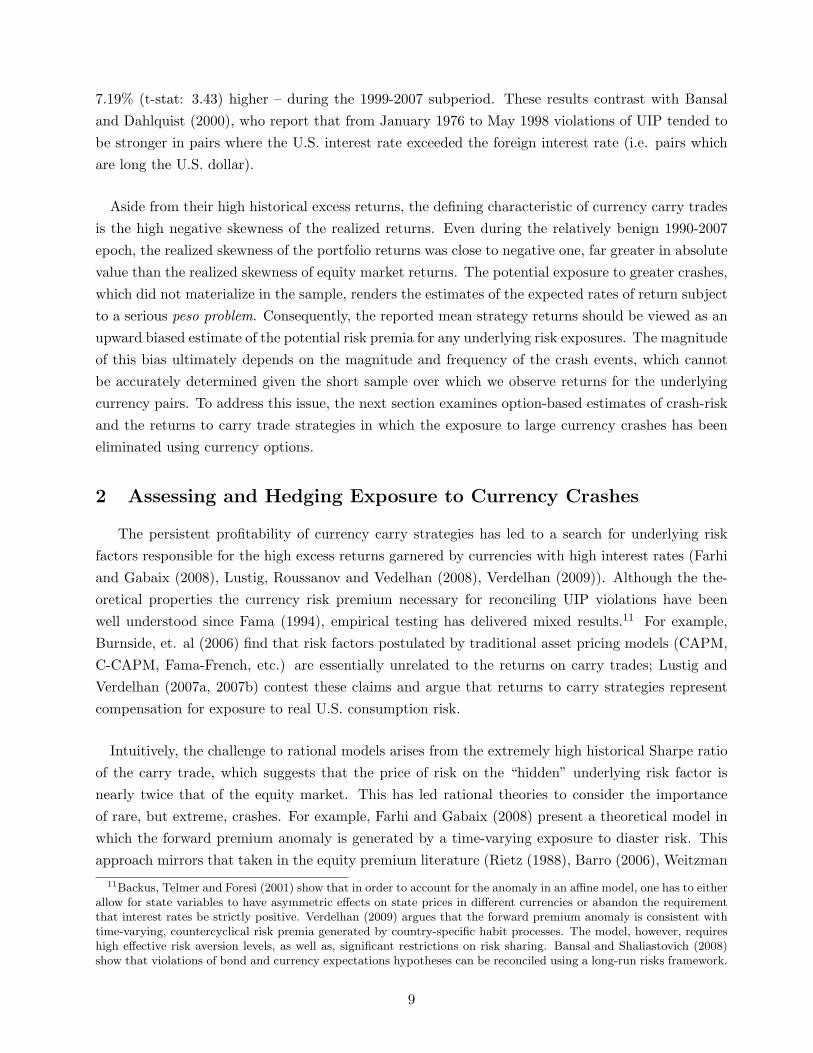
7.19% (t-stat: 3.43) higher – during the 1999-2007 subperiod. These results contrast with Bansaland Dahlquist (2000), who report that from January 1976 to May 1998 violations of UIP tended tobe stronger in pairs where the U.S. interest rate exceeded the foreign interest rate (i.e. pairs whichare long the U.S. dollar).

Aside from their high historical excess returns, the defining characteristic of currency carry tradesis the high negative skewness of the realized returns. Even during the relatively benign 1990-2007epoch, the realized skewness of the portfolio returns was close to negative one, far greater in absolutevalue than the realized skewness of equity market returns. The potential exposure to greater crashes,which did not materialize in the sample, renders the estimates of the expected rates of return subjectto a serious peso problem. Consequently, the reported mean strategy returns should be viewed as anupward biased estimate of the potential risk premia for any underlying risk exposures. The magnitudeof this bias ultimately depends on the magnitude and frequency of the crash events, which cannotbe accurately determined given the short sample over which we observe returns for the underlyingcurrency pairs. To address this issue, the next section examines option-based estimates of crash-riskand the returns to carry trade strategies in which the exposure to large currency crashes has beeneliminated using currency options.

2 Assessing and Hedging Exposure to Currency Crashes

The persistent profitability of currency carry strategies has led to a search for underlying riskfactors responsible for the high excess returns garnered by currencies with high interest rates (Farhiand Gabaix (2008), Lustig, Roussanov and Vedelhan (2008), Verdelhan (2009)). Although the the-oretical properties the currency risk premium necessary for reconciling UIP violations have beenwell understood since Fama (1994), empirical testing has delivered mixed results.11 For example,Burnside, et. al (2006) find that risk factors postulated by traditional asset pricing models (CAPM,C-CAPM, Fama-French, etc.) are essentially unrelated to the returns on carry trades; Lustig andVerdelhan (2007a, 2007b) contest these claims and argue that returns to carry strategies representcompensation for exposure to real U.S. consumption risk.

Intuitively, the challenge to rational models arises from the extremely high historical Sharpe ratioof the carry trade, which suggests that the price of risk on the “hidden” underlying risk factor isnearly twice that of the equity market. This has led rational theories to consider the importanceof rare, but extreme, crashes. For example, Farhi and Gabaix (2008) present a theoretical model inwhich the forward premium anomaly is generated by a time-varying exposure to diaster risk. Thisapproach mirrors that taken in the equity premium literature (Rietz (1988), Barro (2006), Weitzman

11Backus, Telmer and Foresi (2001) show that in order to account for the anomaly in an affine model, one has to eitherallow for state variables to have asymmetric effects on state prices in different currencies or abandon the requirementthat interest rates be strictly positive. Verdelhan (2009) argues that the forward premium anomaly is consistent withtime-varying, countercyclical risk premia generated by country-specific habit processes. The model, however, requireshigh effective risk aversion levels, as well as, significant restrictions on risk sharing. Bansal and Shaliastovich (2008)show that violations of bond and currency expectations hypotheses can be reconciled using a long-run risks framework.

9

(2007), Martin (2008)) and the literature seeking to reconcile the prices of deep out-of-the-moneyputs with empirical return distributions (Pan (2002)). Indeed, Coval and Shumway (2001), Bakshiand Kapadia (2003), and Driessen and Maenhout (2006) report high Sharpe ratios for various delta-neutral option strategies, which can be interpreted as being consistent with large volatility and crashrisk premia. Consequently, exposure to a highly priced crash risk factor attaching to currencies withrelatively high interest rates provides a plausible mechanism for explaining the observed violationsof uncovered interest parity.

In order to examine the crash risk hypothesis, I turn to data on foreign exchange (FX) options andbegin by introducing methodologies used to assess and hedge exposure to currency crashes. The priceof options protecting against the risk of rapid devaluations provides valuable information regardingthe probability of currency crashes, as well as, the risk premia demanded by investors for beingexposed to those risks. To examine the market’s ex ante perceptions of crash risk, I first use theoption data to extract the moments of the risk-neutral distribution. A comparison of the dynamics ofthe risk-neutral moments – in particular risk-neutral skewness – vis a vis realized skewness, providessurprising insights regarding the market’s time-varying perceptions of tail risk. Finally, I introducethe construction of crash-neutral currency carry trades, in which exposure to rapid depreciations(appreciations) of the high (low) interest rate currencies has been hedged in the option market. Toassess whether violations of UIP are attributable to crash risk premia, the empirical section comparesthe excess returns to the crash-neutral strategies with the returns obtained from the unhedged carrystrategy.

2.1 The market’s perception of crash risk

Breeden and Litzenberger (1978) were the first to show that an asset’s entire risk-neutral distri-bution (i.e. state price density) can be recovered from the prices of a complete set of options on thatasset. Following the logic of state-contingent pricing (Arrow (1964), Debreu (1959)), the risk-neutraldistribution, q(S), enables one to value arbitrary state contingent payoffs, H(S), via the followingpricing equation:

pt = exp(−rd,t · τ) ·∫ ∞

0H(St+τ ) · q(St+τ )dSt+τ (6)

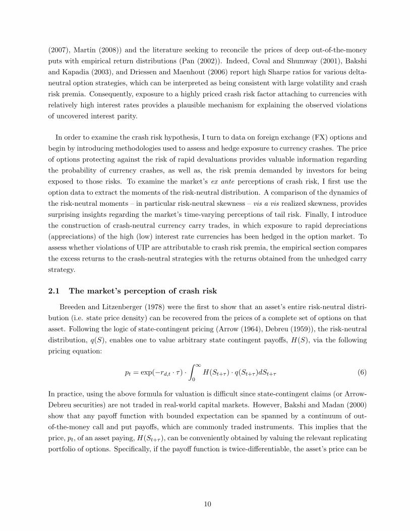
In practice, using the above formula for valuation is difficult since state-contingent claims (or Arrow-Debreu securities) are not traded in real-world capital markets. However, Bakshi and Madan (2000)show that any payoff function with bounded expectation can be spanned by a continuum of out-of-the-money call and put payoffs, which are commonly traded instruments. This implies that theprice, pt, of an asset paying, H(St+τ ), can be conveniently obtained by valuing the relevant replicatingportfolio of options. Specifically, if the payoff function is twice-differentiable, the asset’s price can be

10

obtained from:

pt = exp(−rd,t · τ) · (H(S)− S) +HS(S) · St +

+∫ ∞S

HSS(K) · Ct(K, τ) · dK +∫ S

0HSS(K) · Pt(K, τ) · dK (7)

where K are option strike prices, HS(·) and HSS(·), denote the first and second derivatives of thestate-contingent payoff, and S is some future value of the underlying, typically taken to be theforward price. Intuitively, this expression states that the payoff H(S) can be synthesized by buying(H(S)−S) units of a riskless bond, HS(S) units of the underlying security and a linear combinationof puts and calls with positions given by HSS(K).

Bakshi, Kapadia, and Madan (2003) show that the above approach provides a convenient methodfor computing the risk-neutral moments of the underlying distribution.12 In particular, if we denotethe continuously compounded return by, Rt,τ ≡ lnSt+τ−lnSt, the values of the (non-central) τ -periodmoments under the risk-neutral measure can be simply computed by setting H(St+τ ) = (Rt,τ (St+τ ))n

and removing the discounting. The corresponding discounted values can be interpreted as the pricesof contracts paying the realized (non-central) moments of the distribution. After a few simpletransformations these values can then be converted to the prices of contracts paying the realizedcentral moments (variance, skewness, etc.).

Since the state-contingent payoffs, H(S) = (Rt,τ (St+τ ))n, satisfy the above technical conditions,we can obtain the prices of the non-central moment swaps, by substituting the relevant derivativesinto (7). The expressions for the discounted values of the first three non-central moments, denotedby Vt(τ), Wt(τ) and Xt(τ), are provided in the Appendix. To fix intuition regarding the associatedoption portfolios, Figure 3 plots the option positions, HSS(·), for each of the moment contractsas a function of the option strike value. For example, replication of the second moment requiresestablishing long positions in options at all moneyness levels, with sizes that scale inversely withthe square of the option strike value. As a result, the price of the second moment contract isstrictly positive, and is particularly high whenever the prices of deep out-of-the-money puts are high.The third non-central moment is replicated by a combination of negative positions in out-of-the-money puts and positive positions in out-of-the-money calls. Consequently, whenever the underlyingdistribution is negatively (positively) skewed and the prices of puts are greater than (less than) theprices of calls, the price of the replicating portfolio will be negative (positive). Finally, replicationof the contract paying the realized fourth moment, once again entails strictly positive positions inoptions of all moneyness values, but now more heavily weighed in the tails.

When applied to data on foreign exchange options, this framework facilitates the dynamic com-putation of the risk-neutral moments of the option-implied currency return distribution, resulting

12This approach is effectively an extension of the early results in Britten-Jones and Neuberger (2000) and Carr andMadan (2001) for the pricing of variance swaps.

11

in a daily time series of option-implied variance, skewness and kurtosis observations. Importantly,the time variation in option-implied skewness provides a direct way for assessing the market’s time-varying perceptions of crash risk, and the cost of insuring against extreme currency moves. In Section4, I characterize the behavior of risk-neutral skewness in relation to the actual realized skewness,and relate both to measures of the attractiveness of currency carry trades (e.g. interest rate dif-ferentials), as well as, recent currency moves. I find that the realized and option-implied skewnessmeasures exhibit dramatically different behavior. While future realized skewness is negatively relatedto past currency appreciations, suggesting that appreciated currencies are more likely to crash, therisk-neutral skewness is positively related to past currency appreciations, suggesting that the marketperceives appreciated currencies as less likely candidates for a crash. As a result, insurance againstcrash risk becomes least expensive, precisely as the risk of a crash increases.

2.2 Crash-neutral currency carry trades

In order to provide a returns-based measure of the crash risk premium, I also construct carrytrades in which the spot currency positions of the standard currency carry trade are combined witha position in a foreign exchange (FX) option. The option position is chosen such that the risk ofextreme negative outcomes stemming from a depreciation (appreciation) of the high (low) interestrate currency is entirely eliminated. More precisely, whenever the foreign short-term instrument isthe long leg of the trade, an investor seeking to limit exposure to sudden depreciations purchases aput option on the foreign currency. Conversely, if the carry trade is funded in the foreign currency, aninvestor seeking to limit downside exposure purchases a call option, limiting the risk from a suddenappreciation. I refer to these downside-protected trades as crash-neutral carry trades. They areconstructed to have two features: (1) conditional on the option protection expiring in-the-money allcurrency risk exposure is eliminated; and, (2) the currency exposure of the crash-neutral portfoliomatches that of the standard carry trade (i.e. the delta exposure of the option is hedged at initiation).Intuitively, the first condition ensures that exposure to crash risk is entirely eliminated, while thesecond, ensures that the returns from the crash-neutral carry strategies are directly comparable withthose from the standard strategy presented in Section 1. To test whether the excess returns to thecurrency carry trade can be attributed to a crash risk premium, I compare the standard carry tradeto three variants of the crash-neutral carry trade, differing in the amount of downside protectionoffered by the option overlay.13 The returns to portfolio strategies combining crash-neutral tradescomplement the analysis of risk-neutral moments, and indicate that between 15% and 35% of theexcess returns to standard carry trades may indeed be interpreted as compensation for exposure tocurrency crashes. Before turning to the data, however, I provide a detailed description of how thecrash-neutral carry trades are constructed.

13Burnside, et al. (2008) construct similar currency strategies, however, their panel contains a smaller cross-sectionof countries and only examines carry trades hedged using at-the-money options. Since the focus is on eliminatingexposure to extreme moves, deep out-of-the-money options are more relevant, as they provide the most direct measureof the cost of insuring against crashes. Moreover, since their strategies do not hedge the delta exposure of the optionoverlay the returns cannot be directly compared with returns from the unhedged carry trade.

12

2.2.1 Portfolio construction

First, consider the situation when the foreign interest rate, rf,t, exceeds the domestic interestrate, rd,t. In order to take advantage of the deviation from UIP, the trader would like to establisha long position in the foreign currency. In the standard carry trade, this long position exposes thecarry trader to losses in the event of a sudden depreciation of the foreign currency. To protect againstthese losses the carry trader can purchase FX puts with a strike price of Kp at a cost of Pt(Kp, τ)dollars per put. If the carry trader purchases qp puts, he must also purchase an additional −q · δpunits of the foreign currency, to hedge the negative delta of the put options. Consequently, if thetrader started by buying one unit of the foreign currency – as in (5) – he must now buy an additionalqp · δp units of the foreign currency. To fund this position he must borrow an additional qp · δp · Stin his domestic currency. Finally, we assume the purchase price of the puts is covered by borrowingadditional funds in the domestic currency. At time t+ 1 the payoff to this portfolio is given by:

CTCN

t+1(rf,t > rd,t) = exp(rf,t · τ) · (1− qp · δp) · St+1 + qp ·max(Kp − St+1, 0)−

− exp(rd,t · τ) · ((1− qp · δp) · St + qp · Pt(Kp, τ)) (8)

In order to eliminate all currency exposure below the strike price of the option, Kp, the quantity ofputs must satisfy,

qp = exp(rf,t · τ) · (1− qp · δp) → qp =exp(rf,t · τ)

1 + exp(rf,t · τ) · δp(9)

With the above quantity restriction, the payoff equation can be re-expressed as:

CTCN

t+1(rf,t > rd,t) = qp ·max(Kp, St+1)− exp(rd,t · τ) · ((1− qp · δp) · St + qp · Pt(Kp, τ)) (10)

This expression makes transparent that the payoff to the strategy is bounded from below, and thatfor terminal realizations of the exchange rate that are above Kp, the strategy payoff response issteeper than in the standard carry trade. In the standard carry trade the sensitivity to changes inSt+1 is equal to exp(rf,t · τ), whereas in the crash-neutral strategy it is given by qp which is strictlygreater than exp(rf,t · τ) since δp < 0. The payoff to the crash-neutral carry trade is illustrated vis avis the payoff to the standard carry trade in the left panel of Figure 5. The crash-neutral carry tradeis assumed to include a put option struck 2.5% out-of-the-money relative to the prevailing forwardrate (KpFt = 0.9750).

By simultaneously decreasing exposure to depreciations (crashes) of the high interest rate currencyand increasing exposure to its appreciations, the crash-neutral strategy is able to maintain the sameunconditional ex ante exposure as the standard carry trade, as desired. Moreover, as the put is struckprogressively further out-of-the-money and offers less protection, the delta of the put converges tozero, causing the upside exposure of the crash-neutral trade, qp, to converge to that of the standardcarry trade. In this sense, the crash-neutral strategy nests the payoff to the standard carry strategy.

13

Now consider the situation when the domestic interest rate, rd,t, exceeds the foreign short rate,rf,t. In order to take advantage of the UIP violations, the investor borrows $1 in foreign currencyand invests the proceeds in a combination of the short-term domestic bonds and FX calls. Becausethe position involves borrowing at the foreign short rate it is effectively short the foreign currency,and the call options limit its downside exposure. Suppose the investor were to buy, qc calls witha strike price of Kc, at a price of Ct(Kc, τ) dollars per call. In order to eliminate the additionalexposure stemming from the long position in the calls (δc > 0), the investors shorts q · δc units of theforeign currency in addition to the baseline short position of one unit (as in the standard currencycarry trade). Finally, the investor funds the purchase of the call options by borrowing the funds atthe domestic interest rate, rd,t.14 At time t+ 1 the payoff to the portfolio is:

CTCN

t+1(rd,t > rf,t) = exp(rd,t · τ) · ((1 + qc · δc) · St − qc · Ct(Kc, τ)) + qc ·max(St+1 −Kc, 0)−

− exp(rf,t · τ) · (1 + qc · δc) · St+1 (11)

Once again, the requirement that all currency exposure be eliminated above Kc implies that the callquantity satisfy:

qc = exp(rf,t · τ) · (1 + qc · δc) → qc =exp(rf,t · τ)

1− exp(rf,t · τ) · δc(12)

which allows us to simplify the payoff to:

CTCN

t+1(rd,t > rf,t) = exp(rd,t · τ) · ((1 + qc · δc) · St − qc · Ct(Kc, τ))− qc ·min(Kc, St+1) (13)

The payoff makes clear that the portfolio is protected against appreciations of the low interest foreigncurrency beyond the strike price of the option Kc. By contrast, relative to the standard carry trade,the crash-neutral strategy increases exposure to depreciations of the funding currency. While thepayoff of the standard carry trade responds by exp(rf,t · τ) to moves in the foreign exchange rate,the crash-neutral strategy responds by qc, whenever St+1 remains below Kc. Since δc > 0, one cansee that qc > exp(rf,t · τ). The payoff to this crash-neutral carry trade is illustrated vis a vis thepayoff to the standard carry trade in the right panel of Figure 5. The crash-neutral carry trade isassumed to include a call option struck 2.5% out-of-the-money relative to the prevailing forward rate(KcFt = 1.0250). Once again, as the call option is struck at a progressively higher price, offering lessprotection, its delta converges to zero, such that the payoff to the crash-neutral strategy convergesto the payoff of the standard carry trade.

Finally, to compute the returns to the carry trade we divide the payoffs by the dollar value of thecapital necessary to establish the positions. In the case of the portfolio which includes puts and islong the foreign currency, the funding capital is (1− qp · δp)·St+qp ·Pt(Kp, τ). For the portfolio which

14Formally, the investor could fund the purchase of the calls at the lower, foreign interest rate. The assumption offunding at the domestic rate is made to preserve the symmetry of the solution, which is lost when additional currencyrisk is borne by the investor when he funds the purchase of the calls at the foreign rate.

14

is long the domestic currency and includes calls, the funding capital is (1 + qc · δc) ·St−qc ·Ct(Kc, τ).When the quantity of options in the portfolio goes to zero, the funding capital goes to St in bothcases, as in the case for the standard carry trade. Intuitively, the standard carry trade is simplythe limiting case of the crash-neutral trade as we let the strike price of the put (call) diverge tozero (infinity). In these cases, the prices of the FX options go to zero, and the two strategies offeridentical payoffs.

3 Data

The results in this paper are based on two datasets. The first dataset contains information on one-, three-, six-month and one-year Eurocurrency (LIBOR) rates and was obtained from Datastream.Eurocurrency rates are the interest rates at which banks are willing to borrow and lend foreigncurrency deposits, and constitute the effective interest rates at which a carry trade investor wouldbe able to borrow and lend. The LIBOR rates published by Datastream are from daily fixings ofthe British Bankers Association (BBA). The data are daily and cover the period from January 1990through December 2008. In the event that BBA interest rate data are unavailable for the entire timeperiod, the BBA series is spliced with the corresponding interbank lending rate published by thecountry’s central bank, provided through Datastream or Global Financial Data. Time series meansof the one-month LIBOR rates are reported in Panel A of Table III. Daily exchange rates for thenine G10 currencies versus the U.S. dollar are obtained from Reuters via Datastream.

The second dataset, the foreign exchange (FX) option dataset, is comprised of daily impliedvolatility quotes at five strikes and four maturities for options on the G10 currencies and fifteenemerging currency pairs. The exchange rate options are European and give their owners the right tobuy or sell a foreign currency at a pre-specified exchange rate measured in U.S. dollars per unit offoreign currency. The data on exchange rate options was obtained from J.P. Morgan and covers theperiod from January 1999 to December 2008. I begin by introducing some formalisms specific to theforeign exchange option markets, characterizing the structure of implied volatilities, and describingthe procedure for converting the implied volatility data into observations of risk-neutral moments.

3.1 Foreign exchange options

FX option prices are quoted in terms of their Garman-Kohlhagen (1983) implied volatilities,much like equity options are quoted in terms of their Black-Scholes (1973) implied volatilities. Infact, the Garman-Kohlhagen valuation formula is equivalent to the Black-Scholes formula adjustedfor the fact that both currencies pay a continuous “dividend” given by their respective interest rates.The price of a call and put option can be recovered from the following formulas:

Ct(K, τ) = e−rd,t·τ ·[Ft,τ ·N(d1)−K ·N(d2)

](14a)

Pt(K, τ) = e−rd,t·τ ·[K ·N(−d2)− Ft,τ ·N(−d1)

](14b)

15

where:

d1 =lnFt,τ/K

σt(K, τ) ·√τ

+12· σt(K, τ) ·

√τ d2 = d1 − σt(K, τ) ·

√τ (15)

and Ft,τ is the forward rate for currency to be delivered τ periods forward, and rf,t and rd,t are theforeign and domestic interest rates for τ -period loans, respectively. The forward rate is determinedthrough the covered interest parity condition, a no-arbitrage relationship which must hold at time t,and is equal to St · exp {(rd,t − rf,t) · τ}. The implied volatilities necessary to match the price of theτ -period options will generally depend on the option’s strike value, K, and are denoted by σt(K, τ).

Unlike equity options which have fixed calendar expiration dates and are quoted at fixed strikeprices, foreign exchange options are generally quoted at constant maturities and fixed deltas. Moreprecisely, market makers quote prices of portfolio of 0.25 and 0.10 delta options (risk reversals andbutterfly spreads), as well as, an at-the-money delta-neutral straddle. The strike price of the straddle,for any given maturity, is chosen such that the deltas of a put and call at that strike are equal, butof opposite sign. From these data, one can compute implied volatilities at five strike values. Thetime-series averages of the option-implied volatilities at the five quoted strikes are reported in PanelA of Table III.

The most frequently traded options have maturities of 1M, 3M, 6M an 1Y, and include at-the-money options, as well as, calls and puts with deltas of 0.25 and 0.10 (in absolute value). The optiondeltas, obtained by differentiating the option value with respect to the spot exchange rate, St, aregiven by,

δc(K) = e−rf,t·τ ·N(d1) (16a)

δp(K) = −e−rf,t·τ ·N(−d1) (16b)

allowing for conversion between the strike price of an option and its corresponding delta. Specifically,the strike prices of puts and calls with delta values of δp and δc, respectively, are given by:

Kδc = Ft · exp(

12σt(δc)2 · τ − σt(δc) ·

√τ ·N−1 [exp(rf,t · τ) · δc]

)(17a)

Kδp = Ft · exp(

12σt(δp)2 · τ + σt(δp) ·

√τ ·N−1 [− exp(rf,t · τ) · δp]

)(17b)

The strike price of the delta-neutral straddle is obtained by setting δc(K) + δp(K) = 0 and solvingfor K. It is straightforward to see that the options in this portfolio must both have deltas of 0.50(in absolute value), and the corresponding strike value is:

KATM = St · exp(

(rd,t − rf,t) · τ −12σt(ATM)2 · τ

)= Ft · exp

(12σt(ATM)2 · τ

)(18)

16

Consequently, although the straddle volatility is described as “at-the-money,” the correspondingoption strike is neither equal to the spot price or the forward price. In the data, the one-month0.25 delta options are roughly 1.5-2.5% out-of-the-money, and the one-month 0.10 delta optionsare roughly 3.0-4.5% out-of-the-money (Table III, Panel B). When normalized by the at-the-moneyimplied volatility (converted to monthly units), the strikes of the 0.25 delta options are 0.70 standarddeviations away from the forward price, and the 0.10 delta options are about 1.40 standard deviationsaway from the forward price. Finally, in standard FX option nomenclature an option with a deltaof δ is typically referred to as a |100 · δ| option. For example, a put with δ = −0.10, is referred to asa 10δ put. I use this convention from hereon.

3.2 Extracting the risk-neutral moments

The formulas for the risk-neutral moments derived in Section 2 assume the existence of a contin-uum of out-of-the-money puts and calls. In reality, of course, the data are available only at a discreteset of strikes spanning a bounded range of strike values, [Kmin,Kmax], such that any implementationof the moment formulas provides only an approximation to the true risk-neutral moments. It istherefore important to ensure that the available data are adequate to obtain a credible estimate ofthe underlying moments.

Jiang and Tian (2005) investigate these types of approximation errors in the context of computingestimates of the risk-neutral variance from observations of equity index option prices. To address thisissue the authors simulate data from various types of models for the underlying asset and then seekto reconstruct the risk-neutral variance from a discrete set of observed option prices. They examinethe impact of having observations on a finite number of options with a bounded range of strikes, aswell as, the impact of various interpolation and extrapolation procedures. They conclude that thediscreteness of available strikes is not a major issue, and that estimation errors decline to 2.5% (0.5%)of the true volatility when the most deep out-of-the-money options are struck at 1 (1.5) standarddeviations away from the forward price. With options struck at two standard deviations away fromthe forward price, approximation errors essentially disappear completely. Moreover, their resultsindicate that approximation errors are minimized by interpolating the option implied volatilitieswithin the observed range of strikes, and extrapolating the option implied volatilities below Kmin

and above Kmax by appending flat tails at the level of the last observed implied volatility. Consistentwith intuition, they find that this form of extrapolation is preferred to simply truncating the rangeof strikes used in the computation. Carr and Wu (2008) follow a similar protocol in their study ofvariance risk premia in the equity market, and combine linear interpolation between observed impliedvolatilities with appending flat tails beyond the last observed strikes.

Guided by the sensitivity results in Jiang and Tian (2005), the available cross-section of foreignexchange options is deemed to be sufficiently broad to ensure that the error in extracting the risk-neutral moments is likely to be very small. The furthest out-of-the-money puts and calls are struckat roughly 1.4 times the at-the-money implied volatility away from the prevailing forward prices.

17

Before extracting the risk-neutral moments, I augment the data by interpolating the implied volatilityfunctions between the observed data points, and append flat tails beyond the last observed strike. Iinterpolate implied volatilities using the vanna-volga method (Castagna and Mercurio (2007)), whichis the standard approach used by participants in the FX option market.15 The resulting risk-neutralmoments turn out to be largely unaffected by the precise details of the interpolation scheme, andsimilar results obtain if a standard linear interpolation is used, e.g. as in Carr and Wu (2008).

The vanna-volga method is based on a static hedging argument, and essentially prices a non-tradedoption by constructing and pricing a replicating portfolio, which matches all partial derivatives upto second order. In a Black-Scholes world, only first derivatives are matched dynamically, so thereplicating delta-neutral portfolio is comprised only of a riskless bond and the underlying. However,in the presence of time-varying volatility, it is necessary to also hedge the vega

(∂CBS

∂σ

), as well

as, the volga(∂2CBS

∂2σ

)and vanna

(∂2CBS

∂σ∂St

). In order to match these three additional moments,

the replicating portfolio must now also include an additional three traded options. Consequently,to the extent that at least three FX options are available, the implied volatilities of the remainingoptions can be obtained by constructing the relevant replicating portfolio, and then inverting itsprice to obtain the corresponding implied volatility. Castagna and Mercurio (2007) show that theinterpolated implied volatility for a τ -period option at strike K obtained from the vanna-volgamethod is approximately related to the implied volatilities of three other traded option with thesame maturity and strikes K1 < K2 < K3 through:

σt(K, τ) ≈ln K2

K · lnK3K

ln K2K1· ln K3

K1

· σt(K1, τ) +ln K

K1· ln K3

K

ln K2K1· ln K3

K2

· σt(K2, τ) +ln K

K1· ln K

K2

ln K3K1· ln K3

K2

· σt(K3, τ) (19)

This formula provides a convenient shortcut for carrying out the interpolation and is known to providevery accurate estimates of the implied volatilities whenever K is between K1 and K3 (Castagna andMercurio (2007)). Extrapolations based on this formula, however, lead to spurious results. Since theabove approximation is essentially quadratic in the log strike, it violates the technical conditions forthe existence of moments under the risk-neutral measure when extrapolated to infinity (Lee (2004)).As mentioned earlier, to avoid these issues I append flat implied volatility tails beyond the lastobserved strikes.

4 Results

In order to investigate the hypothesis that the empirically observed violations of uncovered in-terest parity are attributable to the exposure of high interest rate currencies to rapid depreciations,or crashes, I turn to data on foreign exchange options. Options provide a valuable tool for assessingmarket participants’ perceptions of the underlying currency return distributions, as well as, the risk

15Common approaches in the equity option literature either rely on non-parametric methods (Ait-Sahalia and Lo(1998)) or fit ad hoc functional specifications to the observed data (Shimko (1993), Coval, Jurek and Stafford (2008)).

18

premia that are demanded for insurance against rapid currency moves. If high interest rate curren-cies are indeed more prone to crashes, one would expect any of the following to hold in the optiondata: (a) option-implied skewness should forecast currency excess returns with a negative sign; (b)option-implied skewness should be negatively correlated with interest rate differentials in the timeseries, as well as, the cross section; and (c) strategies in which the exposure to currency crashes hasbeen hedged in the option market should earn zero excess returns. In the 1999-2007 sample I findthat: (a) option-implied skewness does not forecast currency excess returns; (b) option-implied skew-ness is positively related to interest rate differentials in the panel in univariate specifications, and isinsignificant in a multivariate specification; and (c) carry trades in which crash risk has been hedgedcontinue to deliver positive, albeit significantly smaller, excess returns. Taken together, the resultsfor crash-hedged strategies indicate that at most 15-35% of the excess returns to currency carrytrades can be interpreted as compensation for exposure to currency crashes. Simply put, the priceof crash insurance in the currency markets appears to be relatively low, especially when contrastedwith equity markets. In fact, in order for the currency excess returns on crash-hedged strategies tobe driven to zero, the implied volatilities of options hedging against crashes would have to have beenroughly four times higher than what is actually observed during 1999-2007. Finally, the dramaticevents of 2008 – a period during which the unhedged carry trade lost nearly 20% – are consideredseparately in Section 5. I use this period as an event study to evaluate the performance of the crashprotection, contrast the actual dynamics of the carry trade losses with those postulated by modelsbased on rare jumps, and examine alternative hedging strategies.

4.1 Implied volatility functions

Before turning to formal tests of the crash risk hypothesis, it is useful to begin with a briefsummary of the stylized features of the foreign exchange option data. Much like equity options,the implied volatility functions of foreign exchange options – the plots of volatility as a function ofstrike price – exhibit a pronounced smile. Unlike in equities though, where the smile is essentiallystrictly downward sloping, the smile can take on a variety of shapes, suggesting that the risk-neutraldistribution can be either positively or negatively skewed. To summarize these features Figure 6plots the time-series means of the implied volatility functions for the nine G10 currencies. The red(blue) lines correspond to periods in which the foreign short-term interest rate was above (below)the US short-term interest rate. Before taking means the volatilities were re-scaled by the contem-poraneous at-the-money values to ensure a scale free representation. As can be readily seen, theshape of the implied volatility function exhibits significant variation across countries and time. Forexample, the implied volatility functions for the Swiss franc (CHF) and the Japanese yen (JPY)exhibit a right-skewed smile indicating a positively skewed risk-neutral distribution, suggestive ofthe potential for rapid appreciations against the U.S. dollar. During the 1999-2007 period, both ofthese currencies were characterized by low interest rates (time series means: 1.49% (CHF), 0.19%(JPY)), and are anecdotally known to have been popular funding currencies for the carry trade.Conversely, the implied volatility functions for the Australian dollar (AUD) and New Zealand dollar(NZD), which had relatively high interest rates during the sample (time series means: 5.39% (AUD),

19

6.06% (NZD)) and were the target currencies for carry traders, exhibit left-skewed smiles, consistentwith a negatively skewed risk-neutral distributions. In sum, the cross-sectional evidence points tothe fact that the exchange rates of relatively high (low) interest rate currencies expose investors tothe risk of large depreciations (appreciations), consistent with the data in Brunnermeier, Nagel andPedersen (2008). Unconditionally, the risk-neutral distributions of high (low) interest rate currenciesare negatively (positively) skewed, consistent with the crash risk hypothesis.

However, theories of the forward premium puzzle invoking crash risk as the source of the riskpremium attaching to currencies with relatively higher interest rates, also make a prediction aboutthe time series behavior of the implied-volatility smile. In particular, the skewness of the risk-neutraldistribution should change sign conditional on the sign of the interest rate differential. Whenevera currency features an interest rate that is above (below) the U.S. interest rate, the risk-neutralexchange rate distribution should be negatively (positively) skewed. If this were the case, the solidblue lines in Figure 6 would exhibit a steeper slope for moneyness values below at-the-money (depre-ciation) than for moneyness values above at-the-money (appreciation). Symmetrically, the dashedred lines would exhibit a steeper slopes for moneyness values above at-the-money, than for valuesbelow at-the-money. In general, the data do not seem to be supportive of the conditional predictionof the crash risk hypothesis when evaluated from the perspective of a dollar-based investor.

4.2 Risk-neutral moments

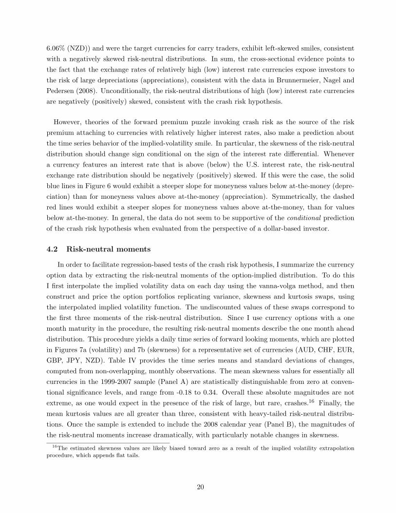
In order to facilitate regression-based tests of the crash risk hypothesis, I summarize the currencyoption data by extracting the risk-neutral moments of the option-implied distribution. To do thisI first interpolate the implied volatility data on each day using the vanna-volga method, and thenconstruct and price the option portfolios replicating variance, skewness and kurtosis swaps, usingthe interpolated implied volatility function. The undiscounted values of these swaps correspond tothe first three moments of the risk-neutral distribution. Since I use currency options with a onemonth maturity in the procedure, the resulting risk-neutral moments describe the one month aheaddistribution. This procedure yields a daily time series of forward looking moments, which are plottedin Figures 7a (volatility) and 7b (skewness) for a representative set of currencies (AUD, CHF, EUR,GBP, JPY, NZD). Table IV provides the time series means and standard deviations of changes,computed from non-overlapping, monthly observations. The mean skewness values for essentially allcurrencies in the 1999-2007 sample (Panel A) are statistically distinguishable from zero at conven-tional significance levels, and range from -0.18 to 0.34. Overall these absolute magnitudes are notextreme, as one would expect in the presence of the risk of large, but rare, crashes.16 Finally, themean kurtosis values are all greater than three, consistent with heavy-tailed risk-neutral distribu-tions. Once the sample is extended to include the 2008 calendar year (Panel B), the magnitudes ofthe risk-neutral moments increase dramatically, with particularly notable changes in skewness.

16The estimated skewness values are likely biased toward zero as a result of the implied volatility extrapolationprocedure, which appends flat tails.

20

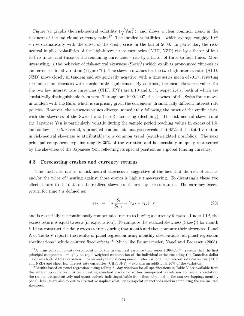
Figure 7a graphs the risk-neutral volatility (√

VarQt ), and shows a clear common trend in theriskiness of the individual currency pairs.17 The implied volatilities – which average roughly 10%– rise dramatically with the onset of the credit crisis in the fall of 2008. In particular, the risk-neutral implied volatilities of the high-interest rate currencies (AUD, NZD) rise by a factor of fourto five times, and those of the remaining currencies – rise by a factor of three to four times. Moreinteresting, is the behavior of risk-neutral skewness (SkewQ

t ) which exhibits pronounced time-seriesand cross-sectional variation (Figure 7b). The skewness values for the two high interest rates (AUD,NZD) move closely in tandem and are generally negative, with a time series mean of -0.17, rejectingthe null of no skewness with considerable significance. By contrast, the mean skewness values forthe two low interest rate currencies (CHF, JPY) are 0.10 and 0.34, respectively, both of which arestatistically distinguishable from zero. Throughout 1999-2007, the skewness of the Swiss franc movesin tandem with the Euro, which is surprising given the currencies’ dramatically different interest ratepolicies. However, the skewness values diverge immediately following the onset of the credit crisis,with the skewness of the Swiss franc (Euro) increasing (declining). The risk-neutral skewness ofthe Japanese Yen is particularly volatile during the sample period reaching values in excess of 1.5,and as low as -0.5. Overall, a principal components analysis reveals that 45% of the total variationin risk-neutral skewness is attributable to a common trend (equal-weighted portfolio). The nextprincipal component explains roughly 30% of the variation and is essentially uniquely representedby the skewness of the Japanese Yen, reflecting its special position as a global funding currency.

4.3 Forecasting crashes and currency returns

The stochastic nature of risk-neutral skewness is suggestive of the fact that the risk of crashesand/or the price of insuring against those events is highly time-varying. To disentangle these twoeffects I turn to the data on the realized skewness of currency excess returns. The currency excessreturn for time t is defined as:

xst = lnStSt−1

− (rd,t − rf,t) · τ (20)

and is essentially the continuously compounded return to buying a currency forward. Under UIP, theexcess return is equal to zero (in expectation). To compute the realized skewness (SkewP

t ) for montht, I first construct the daily excess returns during that month and then compute their skewness. PanelA of Table V reports the results of panel regression using monthly observations; all panel regressionspecifications include country fixed effects.18 Much like Brunnermeier, Nagel and Pedersen (2008),

17A principal components decomposition of the risk-neutral variance time series (1999-2007), reveals that the firstprincipal component – roughly an equal-weighted combination of the individual series excluding the Canadian dollar– explains 65% of total variation. The second principal component – which is long high interest rate currencies (AUDand NZD) and short low interest rate currencies (CHF, JPY) – explains an additional 20% of the variation.

18Results based on panel regressions using rolling 21-day windows for all specifications in Table V are available fromthe author upon request. After adjusting standard errors for within time-period correlation and serial correlation,the results are qualitatively and quantitatively indistinguishable from those obtained in the non-overlapping, monthlypanel. Results are also robust to alternative implied volatility extrapolation methods used in computing the risk-neutralskewness.

21

I find that future values of realized skewness are negatively related to past excess returns and thelagged values of the interest rate spread (rf,t − rd,t). This indicates that currencies that have highinterest rates and have recently appreciated – i.e. have been targets of successful carry trades – aremore likely to experience large negative moves, or crashes. By contrast, the first regression in PanelB, indicates that risk-neutral skewness is strongly positively related to the realized currency return.The existence of a positive relationship is consistent with a risk-based story in which skewness actsas a proxy for a priced risk factor (e.g. as in Farhi and Gabaix (2008)). Namely, as currenciesbecome more negatively (positively) skewed investors charge a greater (smaller) risk premium, andthe currency experiences a contemporaneous depreciation (appreciation).19 However, the evidence onfuture realized skewness appears to suggest that appreciated currencies become riskier, not safer. Asa result, I find that risk-neutral skewness predicts future realized skewness with a negative sign andis highly statistically significant in a univariate specification. Taken together, the evidence suggeststhat the cost of hedging crashes following large appreciations is low, precisely when the risk of acrash is high.

Another result emerging from the panel regressions reported in Panel B is that risk-neutral skew-ness is positively related to the interest rate spread in the univariate panel regression, despite aexhibiting a strong negative relationship in the cross section. This indicates that periods of abnor-mally high spreads are associated with more positive values of risk-neutral skewness, contrary tothe predictions of the crash risk hypothesis. Consistent with Brunnermeier, Nagel and Pedersen(2008), however, I find that this relationship becomes negative, but statistically insignificant in amultivariate specification. Judging by the dramatic difference between the values of the adjusted R2

gross and net of the fixed effects during this time period, risk-neutral skewness appears to be morea fixed feature of a country, rather than a feature of its time-varying interest rate environment.

Finally, if violations of uncovered interest parity (UIP) are attributable to crash risk premia,the magnitude of risk-neutral skewness – a proxy of the market’s crash expectation – would beexpected to forecast currency excess returns with a negative sign. Panel C of Table V investigatesthe forecastability of one-month excess returns, using lagged excess returns, interest rate spreads, aswell as, realized and option-implied measures of skewness. I find a minute amount of momentumin excess returns at the monthly horizon and positive predictability on the basis of the interest ratedifferential. Not only does the option-implied skewness measure not forecast currency excess returns,it appears in the forecasting regression with a positive, albeit insignificant, regression coefficient.

4.4 Crash-neutral carry trade strategies

In order to determine whether the excess returns to carry trades can be attributed to compen-sation for exposure to currency crashes, I turn to an analysis of crash-neutral carry trades. Sincethese trades eliminate exposure to currency crashes by establishing a protective position in foreign

19An alternative hypothesis is that following appreciations (depreciations) there is an imbalance in the demand forcall (put) options, creating price pressure in the option market.

22

exchange options, their mean excess returns should be lower than those of the standard carry trade.In the event that crash risk accounts for the entirety of the observed violations of UIP, excess returnsto crash-neutral carry trades would be statistically indistinguishable from zero. To construct a timeseries of returns for the crash-neutral carry trades – implemented in each of the nine individual cur-rency pairs – I proceed by analogy to the approach used in the standard carry trade. At each monthend, I compare the prevailing one-month interbank lending rates, and establish the relevant positionsin the spot markets and one-month foreign exchange options prescribed by (10) and (13). These po-sitions are then held until the end of the following month, when the option expires. I constructthree variants of the crash-neutral strategy, each offering a different amount of crash protection, asreflected by the strike price (delta) of the included FX option. The summary statistics for thesestrategies are presented in Table VI. Panel A presents the results for crash-neutral strategies using“deep” out-of-the-money options (10δ calls and puts), which only provide protection against movesthat are greater than roughly 1.4 times the magnitude of the monthly standard deviation. Panel Bpresents results for crash-neutral strategies employing options with intermediate moneyness levels(25δ calls and puts), and finally, Panel C presents the results for strategies using at-the-money op-tions. Crucially, note that since the crash-neutral strategies only employ options for which tradableprice data are available in the J. P. Morgan dataset, the accrued strategy returns represent returnsthat were attainable in the marketplace (before transaction costs). The results in this section do notrely on the implied volatility interpolation procedure used in the previous sections whatsoever.

4.4.1 Individual currency pairs

It is immediate from Panel A of Table VI that the addition of crash protection using 10δ optionshas a limited effect on the realized risk-return profile of the currency carry trade. Consistent withintuition, the addition of the crash-protection via the FX option causes the realized returns to be morepositively skewed, and the magnitude of the minimal monthly returns to decline relative to standardcarry trades. Similarly, one also observes a minor decline in the annualized standard deviation of thereturns, although the level of volatility is still high and close to 10%. All four individual currencypairs (AUD, EUR, NZD, SEK) that delivered positive and statistically significant excess returns atthe 5% level in the standard carry trade strategy continue to do so in the crash-neutral variant.However, tests comparing returns of the 10δ crash-neutral carry trade with the standard carry trade,also indicate a statistically significant decline in the mean realized return. For the four currency pairswhich individually delivered positive and statistically significant returns, the mean returns declineby -1.29% (AUD; t-stat: -4.52), -1.12% (EUR; t-stat: -3.62), -0.73% (NZD; t-stat: -1.13) and -0.95%(SEK; t-stat: -2.11) per year. Shifting to crash-neutral strategies with more protection (25δ; PanelB) causes a further decline in the realized returns and a coincident increase in skewness. Now allnine individual currency pairs have positively skewed excess returns, with monthly skewness valuesranging from 0.20 (CHF) to 0.76 (NOK). Eight of those continue delivering positive excess returns,four of which are statistically significant at the 5%-level. When compared with the standard carrytrades, the mean returns decline by -2.04% (AUD; t-stat: -2.10), -2.71% (EUR; t-stat: -3.37), -1.72%(NZD; t-stat: -1.26) and -2.82% (SEK; t-stat: -3.00), respectively.

23

Finally, Panel C of Table VI presents the corresponding summary statistics for crash-neutral cur-rency strategies constructed from positions in the spot currency markets and at-the-money options.With ATM options, the strike price of the option is slightly above the forward exchange rate, and thecarry trader effectively pays up front for protection against all negative deviations from uncoveredinterest rate parity. In other words, the investor locks in the interest rate differential (carry) andretains the upside from potential currency moves in exchange for the option premium. By construc-tion, the returns to these strategies are extremely positively skewed, with monthly skewness valuesgenerally above one. However, there is a significant decline of excess returns in comparison to to thestandard carry trades, with excess returns declining anywhere from -1.01% (CHF) to -5.40% (SEK)per year. Nonetheless, even with ATM hedging, the excess returns to the crash-neutral carry tradeimplemented in the AUD (t-stat: 2.18) and SEK remain statistically significant (t-stat: 1.98) at the5% level.

4.4.2 Portfolio strategies

To summarize the findings for crash-neutral currency carry trades for the 1999-2007 sample, Ionce again construct equal- and spread-weighted portfolios (EQL and SPR), as well as, their dollar-neutral counterparts (EQL-$N and SPR-$N). The returns to the non-dollar-neutral strategies arereported in Panel A of Table VII, and their dollar-neutral counterparts are reported in Panel B. Thistime an interesting dichotomy emerges depending on the method of construction. While the excessreturns to the non-dollar-neutral portfolio remain positive and highly statistically significant in fiveof the six cases, the returns to the dollar-neutral portfolios are statistically distinguishable from zeroonly in one of the six cases. Consequently, the returns to simple equal- and spread-weighted currencycarry trades (Table IIb, Panel B) appear to represent a joint premium for crash risk and net (short)exposure to the U.S. dollar. Moreover, once the sample is extended through the end of 2008 (SectionV), even the excess returns to non-dollar-neutral trades become marginally significant.

During the 1999-2007 sample, only the excess returns on the portfolios that have not been con-strained to have a zero net exposure to the U.S. dollar remain positive and highly statisticallysignificant. For example, the equal-weighted portfolio of crash-neutral carry trades implemented inthe nine individual currency pairs delivers an annualized excess return of 3.85% (10δ; t-stat: 2.76).As expected, the mean return declines with the level of protection offered by the option to 3.11%(25δ; t-stat: 2.47) and 1.62% (ATM; t-stat: 1.62). As with the unhedged carry trades, the returnson the spread-weighted strategies are somewhat higher and more volatile than the returns to theequal-weighted portfolios. The combination of portfolio diversification and the benefit of optionprotection drive down the annualized volatilities to around 4-5% per year, such that correspondingportfolio Sharpe ratios continue to be large and range from 0.76 to 1.20. Returns to dollar-neutralportfolios are considerably lower, and are statistically significant only for a spread-weighted portfolioof 10δ-hedged carry trades, which delivers an annualized excess return of 4.82% (t-stat: 2.02).

24

The cumulative performance of the three spread-weighted, non-dollar-neutral portfolios of crash-hedged currency carry trades is illustrated in Figure 8. The excess returns through 2007 remainpositive even with the most aggressively crash-hedged strategy (ATM), and only 20% of the cumula-tive profits are eliminated, when the least aggressive crash-hedging strategy (10δ) is employed. Thedeclines in the mean realized returns for the non-dollar-neutral spread-weighted strategies range from-1.13% (t-stat: -5.37) per year for the 10δ-hedged portfolio to -4.80% (t-stat: -4.69) per year for theATM -hedged portfolio. The absolute values of these differences are interpretable as currency crashrisk premia, since they represent the excess returns foregone by eliminating exposure to the risk oflarge currency moves. When measured as a fraction of the excess returns earned by the correspond-ing non-dollar-neutral spread-weighted portfolio (SPR) of unhedged carry trades, the declines onthe 10δ- and 25δ-hedged portfolios represent 15-30% of the total return to the unhedged strategy inthe 1999-2007 period. The declines in excess returns for the equal-weighted portfolios (EQL) aresomewhat smaller in magnitude, but represent a greater fraction of the unhedged strategy return,ranging from 20-35%. For the non-dollar-neutral portfolio, the proportional declines in returns areeven larger and account for 25% (10δ, SPR-$N) to 55% (25δ, EQL-$N) of the excess return.20

Overall, excess returns on non-dollar-neutral portfolios of crash-neutral trades remain positive, pro-viding evidence against the hypothesis that crash risk premia alone account for violations of UIP.However, once net portfolio dollar exposures are constrained to zero, excess returns to crash-neutralcarry trades are essentially eliminated altogether.

4.5 Transaction Costs

Although the preceding section illustrates that hedging crash risk eliminates a considerable por-tion of the excess returns to the currency carry trade, the returns on non-dollar-neutral portfoliosremain statistically significant. I examine whether this conclusion is affected by incorporating sensi-ble estimates of foreign exchange option transaction costs. In particular, since the implied volatilitiesused to price the options used in the crash-neutral portfolio represented midquotes, they did not ac-count for the existence of a bid-ask spread. To address this question, I replicate the returns tothe crash-neutral strategies with perturbed values of the implied volatilities used to price the crashprotection. In particular, I apply a simple multiplicative transformation to the implied volatilities,thus increasing the price of all options being purchased.

To assess the impact of transaction costs I apply a volatility multiplier of 1.1, since bid-ask spreadsin foreign exchange option markets are between ±0.5 − 1% volatility points, and the mean optionimplied volatilities in the sample are on the order of 10%. With this modification, the mean ex-cess returns to the 10δ crash-neutral carry trades remain essentially unchanged. The equal-weighted,non-dollar-neutral portfolio strategy delivers an excess return of 3.42% (t-stat: 2.42), and the spread-weighted portfolio delivers an excess return of 6.15% (t-stat: 3.34), corresponding to a 40 basis pointdecline in realized excess returns to the crash-neutral strategies versus the baseline specification

20Results for the full 1999-2008 sample are comparable, and are available upon request.

25

without transaction costs. Therefore, typical transaction costs are insufficient to eliminate the prof-itability of the non-dollar-neutral portfolios of crash-hedged carry trades.

Relatedly, one would also like to know, what would it have taken – in terms of a shift in optionprices (implied volatilities) – in order for the point estimates of the excess returns to the crash-neutral strategies to have been equal to zero in the historical sample? By varying the impliedvolatility multiplier, I find that in order to eliminate the excess returns to crash-neutral carry tradesrequires implied volatilities that are between twice and four times as large, as the values actuallyobserved in the data. For example, with a multiplier of two, excess returns on the non-dollar-neutral,equal- and spread-weighted portfolios are 1.11% (t-stat: 0.75) and 3.88% (t-stat: 2.04), respectively,and with a multiplier of four, they are – -2.49% (t-stat: -1.64) and 0.07% (t-stat: 0.04), respectively.Consequently, while hedging exposure to crash risk helps provide a partial resolution of the UIPpuzzle, it cannot resolve it entirely without simultaneously implying an enormous mispricing in theforeign exchange option market.

5 The Credit Crisis of 2008

During the 2008 calendar year, the spread-weighted portfolio of unhedged currency carry tradessustained a roughly 20% loss (Figure 8), most of which was concentrated in the second half of thecalendar year, following the demise of Lehman Brothers. This dramatic decline in the performance ofthe carry trade was driven by two factors: (a) the significant net short dollar exposure of the equal-and spread-weighted portfolios (Figure 3) entering this period, combined with the simultaneousappreciation of the U.S. dollar relative to most G10 currencies, and (b) the depreciation of the dollarrelative to the Japanese yen, which all of the portfolios were short.

This extreme event provides a laboratory for evaluating the performance of the proposed crashhedging strategies, relative to other intuitive alternatives. For example, I compare the performanceof the 25δ-hedging rule considered in Section 4 relative to a rule which hedges at a fixed moneyness,rather than a fixed delta. Importantly, a hedging rule based on a fixed delta exposes individualcarry trades to progressively larger losses as volatility rises. Intuitively, fixing the delta of the hedgeimplies that the probability of observing the option expire in-the-money is being held constant,which requires that the distance from the current level to the option strike price increase (decrease)with volatility. This can become particularly problematic if returns become positively autocorrelatedduring declines, or the likelihood of future jumps increases following the initial dislocation. Finally,I examine quarterly buy-and-hold returns to crash-hedged strategies protected using three-monthoptions. To the extent that the market does not anticipate the risk of protracted declines correctly,hedging with longer-dated options may be cheaper than paying a progressively increasing insurancepremium for short-dated protection. Indeed, I show that the returns to the quarterly strategy exceedthe compounded returns of the strategy with monthly rebalancing by about 1-2% per year over thefull 1999-2008 sample period.

26

5.1 Return dynamics

To illustrate the events of the second half of 2008, the monthly buy-and-hold returns to theunhedged carry trade portfolios are tabulated in Panel A of Table VIII. When compared with ahistorical annualized volatility of 4-5% for the 1999-2007 period, the August and September returnsto the equal- and spread-weighted portfolios represent negative 2.5 and 2.7 standard deviation moves,respectively. By the end of September, the implied volatilities on individual currency pairs had risentwofold, to about 20% per year. If we assume that the portfolio volatility is approximately half thatof the underlying currency pairs, the -10% returns of the equal- and spread-weighted portfolios inOctober 2008, represent an additional negative 3.3 standard deviation event. Concurrent with thedecline, implied volatilities rose further to about 30% a year, making the subsequent -2-3% move inNovember seem comparatively minor. Taken individually, these negative returns, while substantial,do not stand out as the the extreme jumps postulated by common option-pricing models. Instead,the “crash” of 2008 actually appears to be better described as a sequence of downward moves, ratherthan a single, extreme jump. This is further borne out by estimates of the first-order autoregressivecoefficient for the returns on equal- and spread-weighted portfolios of currency carry trades. Duringthe 1999-2007 subperiod, the coefficient is 0.07 (t-stat: 0.73) for the equal-weighted portfolio, and0.09 (t-stat: 0.95) for the spread-weighted portfolio. The inclusion of 2008 increases theses estimatesto 0.28 (t-stat: 3.31) and 0.29 (t-stat: 3.48), respectively.

5.2 Fixed moneyness hedging

A key feature of foreign exchange markets in the second half of 2008 was the progressive rise inoption-implied volatilities. As a result of this increase, the moneyness of the fixed-delta options usedin constructing the crash-neutral currency carry trades shifted to strike values that were further out-of-the-money (OTM). In particular, the 25δ puts (Mput) and 25δ calls (Mput), which were roughly2% out-of-the-money through the end of August 2008, were 3.5% out-of-the-money by the end ofSeptember and 5-6% out-of-the-money in October and November (Table VIII, Panel B). The shiftin the moneyness value had the effect of exposing the crash-neutral trade to large moves, preciselyas they were about to arrive, translating into an increasing sequence of losses on the 25δ-hedgedportfolios. To mitigate this feature I construct portfolios of crash-neutral currency carry trades thatare hedged using options with a fixed moneyness (or strike). Specifically, I focus on hedging withoptions that are 2% OTM relative to the forward rate, since these represent the closest analog tothe average 25δ option (Table III, Panel B).21 This ensures that the maximum loss that can besustained on an individual pair is capped at 2%, plus the cost of the option protection. The sequenceof returns to these portfolios is presented in Panel C of Table VIII. As expected, until the spike involatilities in September 2008, portfolios hedged in this manner sustain comparable losses to the 25δhedged portfolios, which are essentially struck at 2% OTM. In the following three months, the 2%OTM hedged portfolios have the benefit of being exposed to lower losses, but also sacrifice more

21The pricing of the 2% out-of-the-money options is done by interpolating the implied volatility function, as inSection 3.2.

27

value by purchasing more expensive (closer to at-the-money) protection. Ultimately, the two effectsappear to roughly cancel out when compared over the full 1999-2008 sample (Table IX, Panels Aand B). The returns to strategies hedged in fixed delta and fixed moneyness space are statisticallyindistinguishable. Nonetheless, it is worth pointing out the subtle differences between these twohedging strategies. Fixed delta hedging is appropriate if one is interested in hedging against moves(“jumps”) that are a constant multiple of a potentially time-varying instantaneous volatility. Bycontrast, fixed moneyness hedging is appropriate if one is interested in limiting the absolute size ofthe possible move.

5.3 Quarterly hedging

Finally, I compare the quarterly buy-and-hold returns on portfolios of currency carry tradeshedged using three-month 25δ options, with the compounded intra-quarterly returns to rolling one-month crash insurance. If the price of short-dated insurance tends to increase following large moves,and this effect is not properly anticipated in option markets, buying longer dated options will be amore cost efficient alternative to using one-month options. Indeed, I find that the strategy based onthree-month options outperforms hedging with one-month options by roughly 1% per year for thenon-dollar-neutral portfolios, and by roughly 2% for the dollar-neutral portfolios (Panels C and D ofTable IX) when measured over the full 1999-2008 sample. The differences in returns are statisticallysignificant at the 5% level for non-dollar-neutral equal-weighted portfolios and all spread-weightedportfolios. Since violations of UIP tend to be most pronounced for short horizons (Chinn andMeredith (2004), Chinn (2006)), extending the investment horizon from one to three months cannotaccount for the observed increase in returns. Furthermore, since returns are compared over the fullnine year sample, the improved performance of the quarterly hedging rule is not due to fortuitoustiming in the rebalancing of the option hedge. In fact, the final rebalance in the sample occurredat the end of September 2008, and required buying three month options immediately after impliedvolatilities experienced a twofold increase relative to the full sample average. The comparison ofreturns for the two hedging frequencies suggests two related explanations. The term structure ofFX option implied volatilities may be failing to ex ante appreciate: (a) the increases in the price ofshort-dated insurance that actually tend to materialize following initial declines, and/or (b) the riskof gradual, but protracted, declines like the one experienced during the fall of 2008.

Standing at the beginning of the sample, an investor who was concerned about the risk of “crashes”– interpreted as extreme, rare events – but had no view on the prices of foreign exchange optionswould have plausibly been indifferent between buying one-month and three-month option protection.Interestingly, the ex post performance of the two strategies turned out to be quite different. Duringthe benign, first nine years of the sample (1990-2007), an investor relying on one-month optionswould have earned an excess return of 5.33% (t-stat: 3.29) on a spread-weighted portfolio of 25δ-hedged trades (Table IX, Panel A). However, once the sample is extended to include 2008 (Table IX,Panels B and D), the excess return drops by nearly 2% and becomes borderline significant (t-stat:

28

1.75-2.03).22 This major decline in the excess return is particularly notable in that it is driven by asingle year, and highlights that the strategy rolling one-month options left the investor exposed tothe type of autocorrelated decline observed in 2008. By contrast, an investor who had hedged usingthree-month, 25δ options would have earned an excess return of 4.63% (t-stat: 2.28; Table IX, PanelD), even after the inclusion of 2008. Unlike the hedging strategy using one-month options, quarterlyhedging protected the investor against the sequence of large, negative moves in the fall of 2008, andthe contemporaneous rise in the cost of insurance.

6 Conclusion

The events of 2008 dramatically alter inference about the profitability and dynamics of currencycarry trades. The addition of a single year to a sample beginning in 1990, causes the Sharpe ratioof the unhedged trade to decline from 0.87 (0.94) to 0.57 (0.66), for the non-dollar-neutral equal-(spread-) weighted portfolios. Due to the autocorrelated nature of the decline and the attendant risein the cost of purchasing one-month insurance, even investors who employed one of the crash-hedgedstrategies suffer during the credit crisis of 2008. Although the protracted sequence of negative,monthly returns sums to a major decline in the carry trade, these dynamics appear at odds withthose postulated by models of extreme, but rare, disasters, when viewed at the monthly frequency.An investor who employed a quarterly hedging strategy would have been able to sidestep the risein the costs of insurance observed during the credit crisis, and would have earned returns that are1-2% higher return in annualized terms than those for the monthly hedging strategy.

Using option data on foreign exchange rates between the U.S. dollar and the other G10 curren-cies, covering the period from January 1999 to December 2008, I show that carry trade portfoliosin which the exposure to currency crashes has been hedged, deliver significantly lower returns thantheir unhedged counterparts. The decline in the excess returns delivered by the crash-neutral port-folios strategies suggests that exposure to currency crashes accounts for 15% to 35% of the excessreturns stemming from violations of UIP in non-dollar-neutral portfolios. However, once portfoliosare constrained to simultaneously maintain a zero net exposure to the U.S. dollar, excess returns tocrash-hedged portfolios become negligible, and statistically indistinguishable from zero. Net dollarexposure is a key determinant of returns to currency carry trades, with significantly higher returnsaccruing to pairs that were short the U.S. dollar. Taken jointly, net U.S. dollar exposure and crashrisk premia account for the majority of the excess returns to currency carry trades deployed in G10currencies.

22Differences in point estimates and t-statistics for the 25δ-hedged strategies reported in Panels A/B and C/D ofTable IX are due to omitting quarters for which not all monthly observations were available.

29

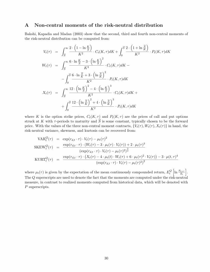
A Non-central moments of the risk-neutral distribution

Bakshi, Kapadia and Madan (2003) show that the second, third and fourth non-central moments ofthe risk-neutral distribution can be computed from:

Vt(τ) =∫ ∞S

2 ·(

1− ln KS

)K2

· Ct(K, τ)dK +∫ S

0

2 ·(

1 + ln SK

)K2

· Pt(K, τ)dK

Wt(τ) =∫ ∞S

6 · ln KS− 3 ·

(ln K

S

)2

K2· Ct(K, τ)dK −

−∫ S

0

6 · ln SK + 3 ·

(ln S

K

)2

K2· Pt(K, τ)dK

Xt(τ) =∫ ∞S

12 ·(

ln KS

)2− 4 ·

(ln K

S

)3

K2· Ct(K, τ)dK +

+∫ S

0

12 ·(

ln SK

)2+ 4 ·

(ln S

K

)3

K2· Pt(K, τ)dK

where K is the option strike prices, Ct(K, τ) and Pt(K, τ) are the prices of call and put optionsstruck at K with τ -periods to maturity and S is some constant, typically chosen to be the forwardprice. With the values of the three non-central moment contracts, {Vt(τ),Wt(τ), Xt(τ)} in hand, therisk-neutral variance, skewness, and kurtosis can be recovered from:

VARQt (τ) = exp(rd,t · τ) · Vt(τ)− µt(τ)2

SKEWQt (τ) =

exp(rd,t · τ) · (Wt(τ)− 3 · µt(τ) · Vt(τ)) + 2 · µt(τ)3

(exp(rd,t · τ) · Vt(τ)− µt(τ)2)32

KURTQt (τ) =

exp(rd,t · τ) ·(Xt(τ)− 4 · µt(t) ·Wt(τ) + 6 · µt(τ)2 · Vt(τ)

)− 3 · µ(t, τ)4

(exp(rd,t · τ) · Vt(τ)− µt(τ)2)2

where µt(τ) is given by the expectation of the mean continuously compounded return, EQt[ln St+τ

St

].

The Q superscripts are used to denote the fact that the moments are computed under the risk-neutralmeasure, in contrast to realized moments computed from historical data, which will be denoted withP superscripts.

30

References

[1] Ait-Sahalia, Yacine and Andrew W. Lo, 1998, Nonparametric estimation of state-price densitiesimplicit in financial asset prices, Journal of Finance, 53, 499-547.

[2] Arrow, Kenneth J., 1964, The Role of Securities in the Optimal Allocation of Risk Bearing,Review of Economic Studies 31, 91-96.

[3] Backus, David K., Silverio Foresi and Chris Telmer, 2001, Affine Term Structure Models andthe Forward Premium Anomaly, 56(1), p. 279-304.

[4] Baillie, Richard T. and Tim Bollerslev, 2000, The Forward Premium Anomaly is Not as Bad asYou Think, Journal of International Money and Finance, 19(4), p. 471-488.

[5] Bakshi, Gurdip and Nikunj Kapadia, 2003, Delta-Hedged Gains and the Negative MarketVolatility Risk Premium, Review of Financial Studies, 16(2), p. 527-566.

[6] Bakshi, Gurdip, Nikunj Kapadia and Dilip Madan, 2003, Stock Return Characteristics, SkewLaws and the Differential Pricing of Individual Equity Options, Review of Financial Studies,16(1), p. 101-143.

[7] Bansal, Ravi and Magnus Dahlquist, 2000, The Forward Premium Puzzle: Different Tales fromDeveloped and Emerging Economies, Journal of International Economics, 51, p. 115-144.

[8] Bansal, Ravi and Ivan Shaliastovich, 2008, A Long-Run Risks Explanation of PredictabilityPuzzles in Bond and Currency Markets, working paper.

[9] Barro, Robert, 2006, Rare Disasters and Asset Markets in the Twentieth Century, QuarterlyJournal of Economics, 121, p. 823-866.

[10] Bates, Davis S., 1996, Dollar Jump Fears, 1984-1992: Distributional Abnormalities Implicit inCurrency Futures Options, Journal of International Money and Finance, 15(1), p. 65-93.

[11] Bhansali, Vineer, 2007, Volatility and the Carry Trade, The Journal of Fixed Income, p.72-84.

[12] Black, Fischer and Myron Scholes, 1973, The pricing of options and corporate liabilities, Journalof Political Economy, 81, p. 617-654.

[13] Breeden, Douglas and Robert Litzenberger, 1978, Prices of state-contingent claims implicit inoption prices, Journal of Business, p. 621-651.

[14] Britten-Jones, M. and A. Neuberger, 2000, Option Prices, Implied Price Processes, and Stochas-tic Volatility, Journal of Finance, 55, p. 839-866.

[15] Brunnermeier, Markus, Christian Gollier, and Jonathan Parker, 2007, Optimal Beliefs, AssetPrices and the Preference for Skewed Returns, American Economic Review (Paper and Proceed-ings), 97(2), p. 159-165.

[16] Brunnermeier, Markus, Stefan Nagel and Lasse Pedersen, 2008, Currency Crashes and the CarryTrade, NBER Macroeconomics Annual, 23, forthcoming.

[17] Burnside, Craig, Martin Eichenbaum, Isaac Kleshchelski and Sergio Rebelo, 2006, The Returnsto Currency Speculation, NBER working paper.

31

[18] Burnside, Craig, Martin Eichenbaum, Isaac Kleshchelski and Sergio Rebelo, 2008, Do PesoProblems Explain the Returns to the Carry Trade?, NBER working paper.

[19] Campa, Jose M, Kevin Chang and Robert Reider, 1998, Implied Exchange Rate Distributions:Evidence from OTC Option Markets, Journal of International Money and Finance, 17(1), p.117-160.

[20] Carr, Peter and Dilip Madan, 2001, Optimal Positioning in Derivative Securities, QuantitativeFinance, 1, p. 19-37.

[21] Carr, Peter and Liuren Wu, 2007, Stochastic Skew in Currency Options, Journal of FinancialEconomics, 86(1), p.213-247

[22] Carr, Peter and Liuren Wu, 2008, Variance Risk Premiums, Review of Financial Studies, forth-coming.

[23] Chinn, Menzie D., 2006, “The (Partial) Rehabilitation of Interest Rate Parity: Longer Horizons,Alternative Expectations and Emerging Markets,” Journal of International Money and Finance,25(1), p. 7-21.

[24] Chinn, Menzie D. and Guy Meredith, 2004, “Monetary Policy and Long Horizon UncoveredInterest Parity,” IMF Staff Papers, 51(3), p. 409-430.

[25] Coval, Joshua D. and Tyler Shumway, 2001, Expected Option Returns, Journal of Finance,56(3), p. 983-1009.

[26] Coval, Joshua D., Jakub W. Jurek and Erik Stafford, 2008, Economic Catastrophe Bonds,American Economic Review, forthcoming.

[27] Castagna, Antonio and Fabio Brigo 2007, Consistent Pricing of FX Options, Risk

[28] Darvas, Zsolt, 2008, Leveraged Carry Trade Portfolios, Journal of Banking and Finance, forth-coming.

[29] Debreu, Gerard, 1959, Theory of Value, New York: Wiley.

[30] DeMiguel, V., L. Garlappi and R. Uppal, 2007, Optimal versus Naive Diversification: HowInefficient Is the 1/N Portfolio Strategy?, Review of Financial Studies, forthcoming.

[31] Driessen, Joost and Pascal Maenhout, 2006, The World Price of Jump and Volatility Risk,working paper.

[32] Engel, Charles, 1996, The Forward Discount Anomaly and the Risk Premium: A Survey ofRecent Evidence, Journal of Empirical Finance, 3, 123192.

[33] Fama, Eugene F., Forward and Spot Exchange Rates, 1984, Journal of Monetary Economics,14, p. 319-338.

[34] Farhi, Emmanuel and Xavier Gabaix, 2008, Rare Disasters and Exchange Rates, working paper.

[35] Farhi, Emmanuel, Samuel P. Fraiberger, Xavier Gabaix, Romain Ranciere and Adrien Verhel-han, 2009, Crash Risk in Currency Markets, working paper.

[36] Frenkel, Jacob A. and Richard M. Levich, 1975, Covered Interest Parity: Unexploited Profits?,Journal of Political Economy, 83(2), p. 325-338.

32

[37] Froot, Kenneth.A, and Richard Thaler, 1990, Anomalies: Foreign Exchange, Journal of Eco-nomic Perspectives, 4, p. 179-192.

[38] Garman, Mark B. and Steven W. Kohlhagen, 1983, Foreign Currency Option Values, Journalof International Money and Finance, 2, p. 231-237.

[39] Hansen, Lars P. and Robert J. Hodrick, 1980, Forward Exchange Rates as Optimal Predictorsof Future Spot Rates: An Econometric Analysis. Journal of Political Economy, 88, p. 829-53.

[40] Jiang, George J. and Yisong S. Tian, 2005, The Model-Free Implied Volatility and Its Informa-tion Content, Review of Financial Studies, 18(4), p. 1305-1342.

[41] Lee, Roger. W., 2004, The Moment Formula for Implied Volatility at Extreme Strikes, Mathe-matical Finance, 14(3), p. 469-480.

[42] Lewis, Karen K., Puzzles in International Financial Markets, in Gene Grossman and KennethRogoff, eds., Handbook of International Economics, Volume 3 (Amsterdam; New York andOxford: Elsevier, North- Holland, 1995).

[43] Lustig, Hanno, and Adrien Verdelhan, 2007a, The Cross-Section of Foreign Currency Risk Pre-mia and US Consumption Growth Risk, American Economics Review, 97(1), p. 89-117.

[44] Lustig, Hanno, and Adrien Verdelhan, 2007b, Note on the Cross-Section of Foreign CurrencyRisk Premia and Consumption Growth Risk, working paper.

[45] Lustig, Hanno, Nick Roussanov and Adrien Verdelhan, 2008, Common Risk Factors in CurrencyMarkets, working paper.

[46] Martin, Ian, 2008, Consumption-Based Asset Pricing with Higher Cumulants, working paper.

[47] Pan, Jun, 2002, The Jump-Risk Premia Implicit in Options: Evidence from an IntegratedTime-Series Study, Journal of Financial Economics, 63, p. 3-50.

[48] Plantin, Guillaume, and Hyun S. Shin, 2008, Carry Trades and Speculative Dynamics, workingpaper.

[49] Rietz, Thomas A., 1988, The Equity Risk Premium: A Solution, Journal of Monetary Eco-nomics, 22, p. 117-131.

[50] Shimko, David, 1993, Bounds of probability, Risk 6, 33–37.

[51] Thompson, Samuel, 2006, Simple Formulas for Standard Errors that Cluster by Both Firm andTime, working paper.

[52] Verdelhan, Adrien, 2008, A Habit-Based Explanation of the Exchange Rate Risk Premium,Journal of Finance, forthcoming.

[53] Weitzman, Martin, 2007, Subjective Expectations and Asset-Return Puzzles, American Eco-nomic Review, 97, p. 1102-30.

33

Table IUIP Regressions.

This table reports coefficient estimates from the regression of the time t+1 log currency return on the time t log forwardpremium,

si,t+1 − si,t = a0 + a1 · (fi,t − si,t) + εi,t+1 H0 : a0 = 0, a1 = 1

Currency returns are computed using 21-day rolling windows and span the period from January 1990 to December 2007(all exchange rates are expressed in terms of dollars per unit of foreign currency). The forward premia are measuredusing the spread between one-month eurocurrency (LIBOR) rates for loans denominated in U.S. dollars and loansdenominated in the foreign currency. The table reports regression coefficients, standard errors (in parentheses), and theχ2 test statistic for the null hypothesis of UIP (p-values in parentheses). Standard errors in individual regressions areadjusted for serial correlation using a Newey-West covariance matrix with 21 lags (1990-2007: N = 4,673; 1999-2007:N = 2,542). The pooled (panel) regression is run with country-fixed effects; the reported standard errors are robust towithin time-period correlation and are adjusted for serial correlation. The pooled regression χ2 statistic is computedfor the null that all country fixed effects are zero and the intercept is equal to one. R2

NFE reports the adjusted R2

from the panel regression net of the fixed effects (1990-2007: N = 42,057; 1999-2007: N = 22,878). XS reportsthe time series means and standard errors of the regression coefficients from cross-sectional regressions performedfor each t. For the cross-sectional regressions R2 is the mean adjusted R2 (1990-2007: N = 4,673; 1999-2007: N = 2,324).

1990-2007 1999-2007Currency a0 a1 R2

NFE χ2 test a0 a1 R2NFE χ2 test

AUD -0.0021 -1.6651 0.0087 9.05 -0.0021 -3.6789 0.0240 9.40(0.0023) (1.0487) (0.01) (0.0036) (1.9450) (0.01)

CAD 0.0006 -0.1754 0.0000 6.87 0.0038 -1.1337 0.0016 5.93(0.0010) (0.5356) (0.03) (0.0016) (2.1465) (0.05)

CHF 0.0027 -1.2094 0.0060 5.20 0.0100 -4.3559 0.0312 8.64(0.0024) (0.9961) (0.07) (0.0041) (1.8256) (0.01)

GBP 0.0006 0.0591 -0.0002 1.28 0.0042 -4.3155 0.0401 11.04(0.0016) (0.8981) (0.53) (0.0023) (1.6417) (0.00)

EUR 0.0021 0.7291 0.0021 3.88 0.0002 -1.6417 0.0053 4.60(0.0018) (1.2675) (0.14) (0.0023) (1.7499) (0.10)

JPY 0.0059 -1.9686 0.0146 11.83 0.0048 -1.5828 0.0070 5.18(0.0025) (0.8638) (0.00) (0.0045) (1.3785) (0.08)

NOK 0.0018 0.7030 0.0052 1.88 0.0017 -1.0765 0.0049 5.42(0.0017) (0.6196) (0.39) (0.0025) (1.2000) (0.07)

NZD -0.0045 -2.4182 0.0131 15.58 -0.0067 -4.7480 0.0406 16.88(0.0034) (1.1961) (0.00) (0.0045) (1.6800) (0.00)

SEK 0.0006 0.6554 0.0053 0.53 0.0031 -3.2701 0.0327 10.35(0.0017) (0.5966) (0.77) (0.0023) (1.3594) (0.01)

Pooled FE -0.0986 0.0000 7.1022 FE -2.7863 0.0190 35.41(0.6500) (0.72) (1.1179) (0.00)

XS 0.0007 -0.1622 0.1161 - 0.0017 -0.5154 0.1157 -(0.0003) (0.0853) (0.0005) (0.1087) -

Table IIaStandard Currency Carry Trade (1990-2007).

Panel A of the table reports summary statistics for returns from implementing the standard carry trade in currency pairsinvolving the U.S. dollar and one of the remaining nine G10 currencies. Returns are in U.S. dollars and are computedmonthly for the period from January 1990 to December 2007 (N = 216). Means, standard deviations and Sharperatios (SR) are annualized. Carry is the mean absolute interest differential between the one-month Eurocurrency ratefor country X and the one-month U.S. dollar rate, |rf,t − rd,t|. Min and Max report the smallest and largest observedmonthly return. Panel B presents analogous summary statistics for portfolios of individual carry trades. The EQLstrategy equal-weights the nine underlying carry trades, whereas SPR weights them by the absolute interest rate spreadat initiation of the trade. The EQL-$N and SPR-$N are constructed analogously, by with the additional requirementthat the portfolio be neutral with respect to exposure to the U.S. dollar.

Panel A: Individual currency pairsAUD CAD CHF EUR GBP JPY NOK NZD SEK

Mean 0.0690 0.0174 0.0149 0.0580 0.0265 0.0444 0.0456 0.0428 0.0793t-stat 3.16 1.19 0.60 2.61 1.23 1.70 1.93 1.91 3.18Std. dev. 0.0927 0.0620 0.1059 0.0942 0.0910 0.1107 0.1003 0.0952 0.1058Skewness -0.18 -0.53 -0.46 -0.35 -0.67 -0.95 -0.24 -0.44 -0.73Kurtosis 2.98 3.86 3.25 3.82 5.54 6.84 3.51 3.84 5.30Min -0.0685 -0.0644 -0.1005 -0.1010 -0.1188 -0.1640 -0.0933 -0.0855 -0.1452Max 0.0891 0.0464 0.0645 0.0755 0.0727 0.1054 0.0756 0.0799 0.0826Carry 0.0206 0.0139 0.0249 0.0206 0.0216 0.0319 0.0256 0.0291 0.0298SR 0.74 0.28 0.14 0.62 0.29 0.40 0.45 0.45 0.75

Panel B: Portfolio strategiesEQL SPR EQL-$N SPR-$N

Mean 0.0442 0.0619 0.0442 0.0692t-stat 3.71 4.00 2.78 3.51Std. dev. 0.0505 0.0657 0.0675 0.0837Skewness -0.91 -0.79 -0.69 -0.80Kurtosis 5.37 4.43 4.75 5.07Min -0.0580 -0.0648 -0.0737 -0.0892Max 0.0375 0.0468 0.0588 0.0651Carry 0.0242 0.0353 0.0370 0.0516SR 0.88 0.94 0.66 0.83N 216 216 180 180

Panel C: Return decompositionPairs short USD Pairs long USD

EQL SPR EQL-$N SPR-$N EQL SPR EQL-$N SPR-$NMean 0.0330 0.0409 0.0425 0.0482 0.0112 0.0210 0.0017 0.0210t-stat 2.96 3.13 2.31 2.42 1.25 1.95 0.08 0.92Std. dev. 0.0472 0.0555 0.0711 0.0814 0.0381 0.0457 0.0814 0.0882Skewness -0.43 -0.42 -0.07 -0.32 -0.31 -0.30 -0.50 -0.47SR 0.70 0.74 0.60 0.50 0.29 0.46 0.02 0.24

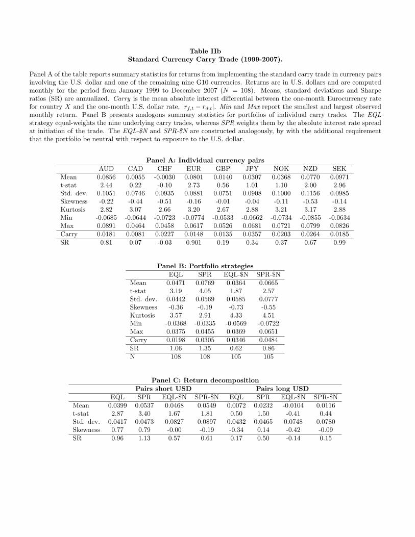
Table IIbStandard Currency Carry Trade (1999-2007).

Panel A of the table reports summary statistics for returns from implementing the standard carry trade in currency pairsinvolving the U.S. dollar and one of the remaining nine G10 currencies. Returns are in U.S. dollars and are computedmonthly for the period from January 1999 to December 2007 (N = 108). Means, standard deviations and Sharperatios (SR) are annualized. Carry is the mean absolute interest differential between the one-month Eurocurrency ratefor country X and the one-month U.S. dollar rate, |rf,t − rd,t|. Min and Max report the smallest and largest observedmonthly return. Panel B presents analogous summary statistics for portfolios of individual carry trades. The EQLstrategy equal-weights the nine underlying carry trades, whereas SPR weights them by the absolute interest rate spreadat initiation of the trade. The EQL-$N and SPR-$N are constructed analogously, by with the additional requirementthat the portfolio be neutral with respect to exposure to the U.S. dollar.

Panel A: Individual currency pairsAUD CAD CHF EUR GBP JPY NOK NZD SEK

Mean 0.0856 0.0055 -0.0030 0.0801 0.0140 0.0307 0.0368 0.0770 0.0971t-stat 2.44 0.22 -0.10 2.73 0.56 1.01 1.10 2.00 2.96Std. dev. 0.1051 0.0746 0.0935 0.0881 0.0751 0.0908 0.1000 0.1156 0.0985Skewness -0.22 -0.44 -0.51 -0.16 -0.01 -0.04 -0.11 -0.53 -0.14Kurtosis 2.82 3.07 2.66 3.20 2.67 2.88 3.21 3.17 2.88Min -0.0685 -0.0644 -0.0723 -0.0774 -0.0533 -0.0662 -0.0734 -0.0855 -0.0634Max 0.0891 0.0464 0.0458 0.0617 0.0526 0.0681 0.0721 0.0799 0.0826Carry 0.0181 0.0081 0.0227 0.0148 0.0135 0.0357 0.0203 0.0264 0.0185SR 0.81 0.07 -0.03 0.901 0.19 0.34 0.37 0.67 0.99

Panel B: Portfolio strategiesEQL SPR EQL-$N SPR-$N

Mean 0.0471 0.0769 0.0364 0.0665t-stat 3.19 4.05 1.87 2.57Std. dev. 0.0442 0.0569 0.0585 0.0777Skewness -0.36 -0.19 -0.73 -0.55Kurtosis 3.57 2.91 4.33 4.51Min -0.0368 -0.0335 -0.0569 -0.0722Max 0.0375 0.0455 0.0369 0.0651Carry 0.0198 0.0305 0.0346 0.0484SR 1.06 1.35 0.62 0.86N 108 108 105 105

Panel C: Return decompositionPairs short USD Pairs long USD

EQL SPR EQL-$N SPR-$N EQL SPR EQL-$N SPR-$NMean 0.0399 0.0537 0.0468 0.0549 0.0072 0.0232 -0.0104 0.0116t-stat 2.87 3.40 1.67 1.81 0.50 1.50 -0.41 0.44Std. dev. 0.0417 0.0473 0.0827 0.0897 0.0432 0.0465 0.0748 0.0780Skewness 0.77 0.79 -0.00 -0.19 -0.34 0.14 -0.42 -0.09SR 0.96 1.13 0.57 0.61 0.17 0.50 -0.14 0.15

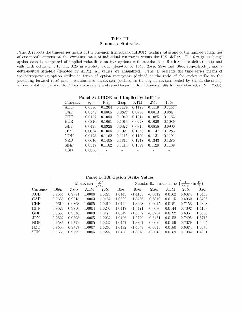
Table IIISummary Statistics.

Panel A reports the time-series means of the one-month interbank (LIBOR) lending rates and of the implied volatilitiesof one-month options on the exchange rates of individual currencies versus the U.S. dollar. The foreign exchangeoption data is comprised of implied volatilities on five options with standardized Black-Scholes deltas: puts andcalls with deltas of 0.10 and 0.25 in absolute value (denoted by 10δp, 25δp, 25δc and 10δc, respectively), and adelta-neutral straddle (denoted by ATM). All values are annualized. Panel B presents the time series means ofthe corresponding option strikes in terms of option moneyness (defined as the ratio of the option strike to theprevailing forward rate) and a standardized moneyness (defined as the log moneyness scaled by the at-the-moneyimplied volatility per month). The data are daily and span the period from January 1999 to December 2008 (N = 2585).

Panel A: LIBOR and Implied VolatilitiesCurrency rf,t 10δp 25δp ATM 25δc 10δcAUD 0.0556 0.1264 0.1179 0.1123 0.1119 0.1155CAD 0.0373 0.0865 0.0822 0.0798 0.0813 0.0847CHF 0.0157 0.1090 0.1049 0.1044 0.1085 0.1153EUR 0.0326 0.1061 0.1013 0.0998 0.1029 0.1089GBP 0.0495 0.0926 0.0872 0.0845 0.0858 0.0900JPY 0.0024 0.1056 0.1021 0.1053 0.1147 0.1283NOK 0.0498 0.1162 0.1115 0.1100 0.1131 0.1191NZD 0.0646 0.1405 0.1311 0.1248 0.1243 0.1280SEK 0.0337 0.1162 0.1114 0.1099 0.1129 0.1189USD 0.0366 - - - - -

Panel B: FX Option Strike Values

Moneyness(KFt

)Standardized moneyness

(1

σATM· ln K

Ft

)Currency 10δp 25δp ATM 25δc 10δc 10δp 25δp ATM 25δc 10δcAUD 0.9553 0.9781 1.0006 1.0225 1.0443 -1.4103 -0.6842 0.0162 0.6874 1.3408CAD 0.9689 0.9845 1.0003 1.0162 1.0322 -1.3766 -0.6810 0.0115 0.6960 1.3706CHK 0.9610 0.9803 1.0005 1.0219 1.0442 -1.3208 -0.6615 0.0151 0.7158 1.4308EUR 0.9621 0.9810 1.0004 1.0207 1.0417 -1.3421 -0.6670 0.0144 0.7092 1.4158GBP 0.9668 0.9836 1.0003 1.0171 1.0342 -1.3827 -0.6784 0.0122 0.6961 1.3830JPY 0.9622 0.9808 1.0005 1.0232 1.0496 -1.2799 -0.6431 0.0152 0.7495 1.5715NOK 0.9586 0.9792 1.0005 1.0227 1.0457 -1.3307 -0.6629 0.0159 0.7079 1.4065NZD 0.9504 0.9757 1.0007 1.0251 1.0492 -1.4079 -0.6818 0.0180 0.6874 1.3373SEK 0.9586 0.9792 1.0005 1.0227 1.0456 -1.3318 -0.6643 0.0159 0.7084 1.4051

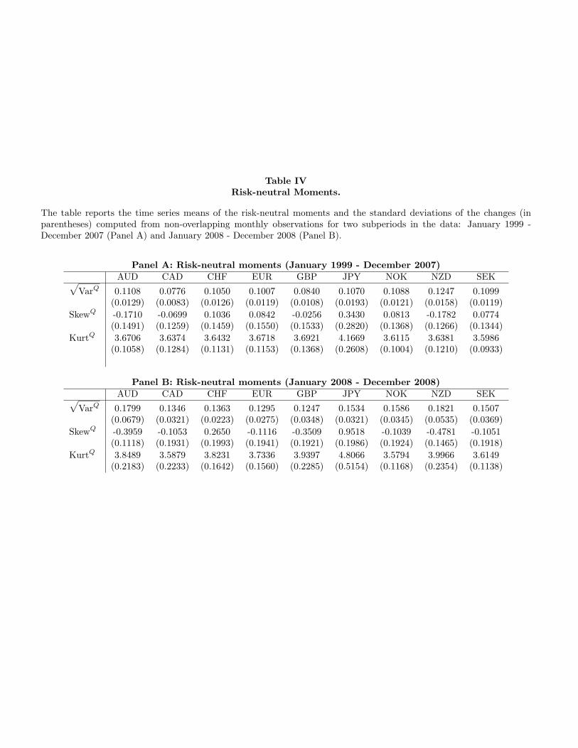
Table IVRisk-neutral Moments.

The table reports the time series means of the risk-neutral moments and the standard deviations of the changes (inparentheses) computed from non-overlapping monthly observations for two subperiods in the data: January 1999 -December 2007 (Panel A) and January 2008 - December 2008 (Panel B).

Panel A: Risk-neutral moments (January 1999 - December 2007)AUD CAD CHF EUR GBP JPY NOK NZD SEK√

VarQ 0.1108 0.0776 0.1050 0.1007 0.0840 0.1070 0.1088 0.1247 0.1099(0.0129) (0.0083) (0.0126) (0.0119) (0.0108) (0.0193) (0.0121) (0.0158) (0.0119)

SkewQ -0.1710 -0.0699 0.1036 0.0842 -0.0256 0.3430 0.0813 -0.1782 0.0774(0.1491) (0.1259) (0.1459) (0.1550) (0.1533) (0.2820) (0.1368) (0.1266) (0.1344)

KurtQ 3.6706 3.6374 3.6432 3.6718 3.6921 4.1669 3.6115 3.6381 3.5986(0.1058) (0.1284) (0.1131) (0.1153) (0.1368) (0.2608) (0.1004) (0.1210) (0.0933)

Panel B: Risk-neutral moments (January 2008 - December 2008)AUD CAD CHF EUR GBP JPY NOK NZD SEK√

VarQ 0.1799 0.1346 0.1363 0.1295 0.1247 0.1534 0.1586 0.1821 0.1507(0.0679) (0.0321) (0.0223) (0.0275) (0.0348) (0.0321) (0.0345) (0.0535) (0.0369)

SkewQ -0.3959 -0.1053 0.2650 -0.1116 -0.3509 0.9518 -0.1039 -0.4781 -0.1051(0.1118) (0.1931) (0.1993) (0.1941) (0.1921) (0.1986) (0.1924) (0.1465) (0.1918)

KurtQ 3.8489 3.5879 3.8231 3.7336 3.9397 4.8066 3.5794 3.9966 3.6149(0.2183) (0.2233) (0.1642) (0.1560) (0.2285) (0.5154) (0.1168) (0.2354) (0.1138)

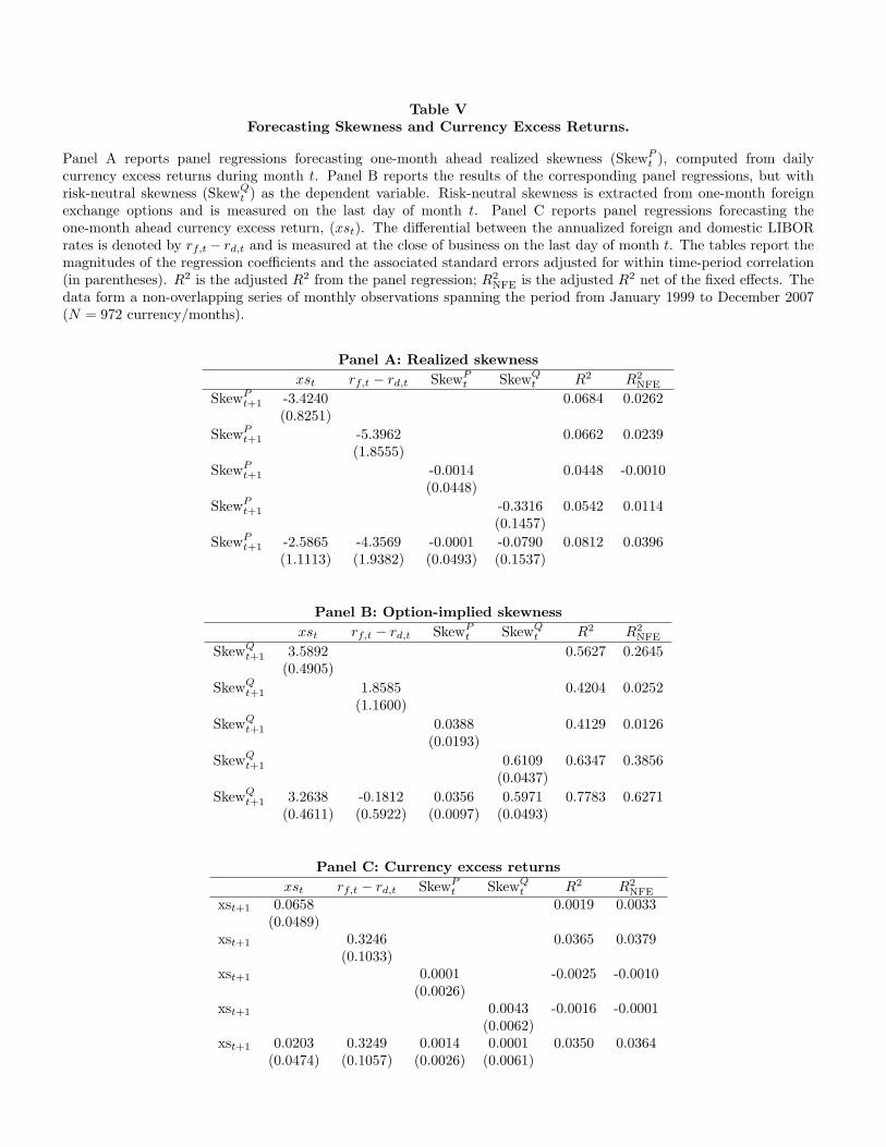
Table VForecasting Skewness and Currency Excess Returns.

Panel A reports panel regressions forecasting one-month ahead realized skewness (SkewPt ), computed from dailycurrency excess returns during month t. Panel B reports the results of the corresponding panel regressions, but withrisk-neutral skewness (SkewQt ) as the dependent variable. Risk-neutral skewness is extracted from one-month foreignexchange options and is measured on the last day of month t. Panel C reports panel regressions forecasting theone-month ahead currency excess return, (xst). The differential between the annualized foreign and domestic LIBORrates is denoted by rf,t − rd,t and is measured at the close of business on the last day of month t. The tables report themagnitudes of the regression coefficients and the associated standard errors adjusted for within time-period correlation(in parentheses). R2 is the adjusted R2 from the panel regression; R2

NFE is the adjusted R2 net of the fixed effects. Thedata form a non-overlapping series of monthly observations spanning the period from January 1999 to December 2007(N = 972 currency/months).

Panel A: Realized skewnessxst rf,t − rd,t SkewPt SkewQt R2 R2

NFE

SkewPt+1 -3.4240 0.0684 0.0262(0.8251)

SkewPt+1 -5.3962 0.0662 0.0239(1.8555)

SkewPt+1 -0.0014 0.0448 -0.0010(0.0448)

SkewPt+1 -0.3316 0.0542 0.0114(0.1457)

SkewPt+1 -2.5865 -4.3569 -0.0001 -0.0790 0.0812 0.0396(1.1113) (1.9382) (0.0493) (0.1537)

Panel B: Option-implied skewnessxst rf,t − rd,t SkewPt SkewQt R2 R2

NFE

SkewQt+1 3.5892 0.5627 0.2645(0.4905)

SkewQt+1 1.8585 0.4204 0.0252(1.1600)

SkewQt+1 0.0388 0.4129 0.0126(0.0193)

SkewQt+1 0.6109 0.6347 0.3856(0.0437)

SkewQt+1 3.2638 -0.1812 0.0356 0.5971 0.7783 0.6271(0.4611) (0.5922) (0.0097) (0.0493)

Panel C: Currency excess returnsxst rf,t − rd,t SkewPt SkewQt R2 R2

NFE

xst+1 0.0658 0.0019 0.0033(0.0489)

xst+1 0.3246 0.0365 0.0379(0.1033)

xst+1 0.0001 -0.0025 -0.0010(0.0026)

xst+1 0.0043 -0.0016 -0.0001(0.0062)

xst+1 0.0203 0.3249 0.0014 0.0001 0.0350 0.0364(0.0474) (0.1057) (0.0026) (0.0061)

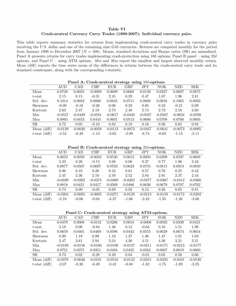
Table VICrash-neutral Currency Carry Trades (1999-2007): Individual currency pairs.

This table reports summary statistics for returns from implementing crash-neutral carry trades in currency pairsinvolving the U.S. dollar and one of the remaining nine G10 currencies. Returns are computed monthly for the periodfrom January 1999 to December 2007 (N = 108). Means, standard deviations and Sharpe ratios (SR) are annualized.Panel A presents returns for carry trades implementing crash-protection using 10δ options; Panel B panel – using 25δoptions, and Panel C – using ATM options. Min and Max report the smallest and largest observed monthly return.Mean (diff) reports the time series mean of the differences in returns between the crash-neutral carry trade and itsstandard counterpart, along with the corresponding t-statistic.

Panel A: Crash-neutral strategy using 10δ-options.AUD CAD CHF EUR GBP JPY NOK NZD SEK

Mean 0.0728 0.0035 -0.0089 0.0689 0.0068 0.0139 0.0327 0.0697 0.0875t-stat 2.15 0.15 -0.31 2.45 0.29 0.47 1.07 1.96 2.81Std. dev. 0.1014 0.0682 0.0866 0.0845 0.0711 0.0888 0.0916 0.1065 0.0933Skewness -0.09 -0.10 -0.26 0.06 0.23 0.05 0.33 -0.21 0.09Kurtosis 2.63 2.47 2.19 2.73 2.40 2.74 2.73 2.58 2.60Min -0.0557 -0.0439 -0.0581 -0.0617 -0.0433 -0.0587 -0.0507 -0.0624 -0.0598Max 0.0865 0.0453 0.0445 0.0601 0.0513 0.0666 0.0708 0.0766 0.0805SR 0.72 0.05 -0.10 0.82 0.10 0.16 0.36 0.65 0.94Mean (diff) -0.0129 -0.0020 -0.0059 -0.0112 -0.0072 -0.0167 -0.0041 -0.0073 -0.0095t-stat (diff) -4.52 -0.49 -1.13 -3.62 -2.09 -8.74 -0.63 -1.13 -2.11

Panel B: Crash-neutral strategy using 25δ-options.AUD CAD CHF EUR GBP JPY NOK NZD SEK

Mean 0.0652 0.0050 -0.0034 0.0530 0.0012 0.0094 0.0209 0.0597 0.0689t-stat 2.23 0.26 -0.15 2.08 0.06 0.37 0.77 1.96 2.43Std. dev. 0.0877 0.0567 0.0697 0.0763 0.0623 0.0755 0.0815 0.0913 0.0850Skewness 0.36 0.43 0.20 0.42 0.61 0.57 0.76 0.25 0.42Kurtosis 2.45 2.36 2.10 2.50 2.52 2.84 2.91 2.37 2.44Min -0.0339 -0.0262 -0.0374 -0.0380 -0.0262 -0.0377 -0.0367 -0.0412 -0.0360Max 0.0818 0.0431 0.0417 0.0569 0.0486 0.0636 0.0679 0.0707 0.0762SR 0.74 0.09 -0.05 0.69 0.02 0.12 0.26 0.65 0.81Mean (diff) -0.0204 -0.0005 -0.0005 -0.0271 -0.0128 -0.0213 -0.0159 -0.0172 -0.0282t-stat (diff) -2.10 -0.06 -0.04 -3.37 -1.66 -2.42 -1.35 -1.26 -3.00

Panel C: Crash-neutral strategy using ATM-options.AUD CAD CHF EUR GBP JPY NOK NZD SEK

Mean 0.0479 0.0008 -0.0131 0.0286 0.0018 -0.0008 0.0033 0.0339 0.0431t-stat 2.18 0.06 -0.84 1.46 0.12 -0.04 0.16 1.51 1.98Std. dev. 0.0659 0.0401 0.0469 0.0586 0.0442 0.0555 0.0629 0.0674 0.0654Skewness 0.99 1.19 0.99 1.10 1.37 1.36 1.47 1.01 1.03Kurtosis 3.47 3.61 2.94 3.24 4.30 4.51 4.36 3.21 3.21Min -0.0189 -0.0156 -0.0180 -0.0196 -0.0127 -0.0211 -0.0171 -0.0213 -0.0177Max 0.0721 0.0375 0.0351 0.0494 0.0425 0.0562 0.0607 0.0619 0.0660SR 0.73 0.02 -0.28 0.49 0.04 -0.01 0.05 0.50 0.66Mean (diff) -0.0378 -0.0046 -0.0101 -0.0516 -0.0122 -0.0315 -0.0335 -0.0431 -0.0540t-stat (diff) -2.07 -0.30 -0.49 -3.42 -0.88 -1.82 -1.75 -1.89 -3.25

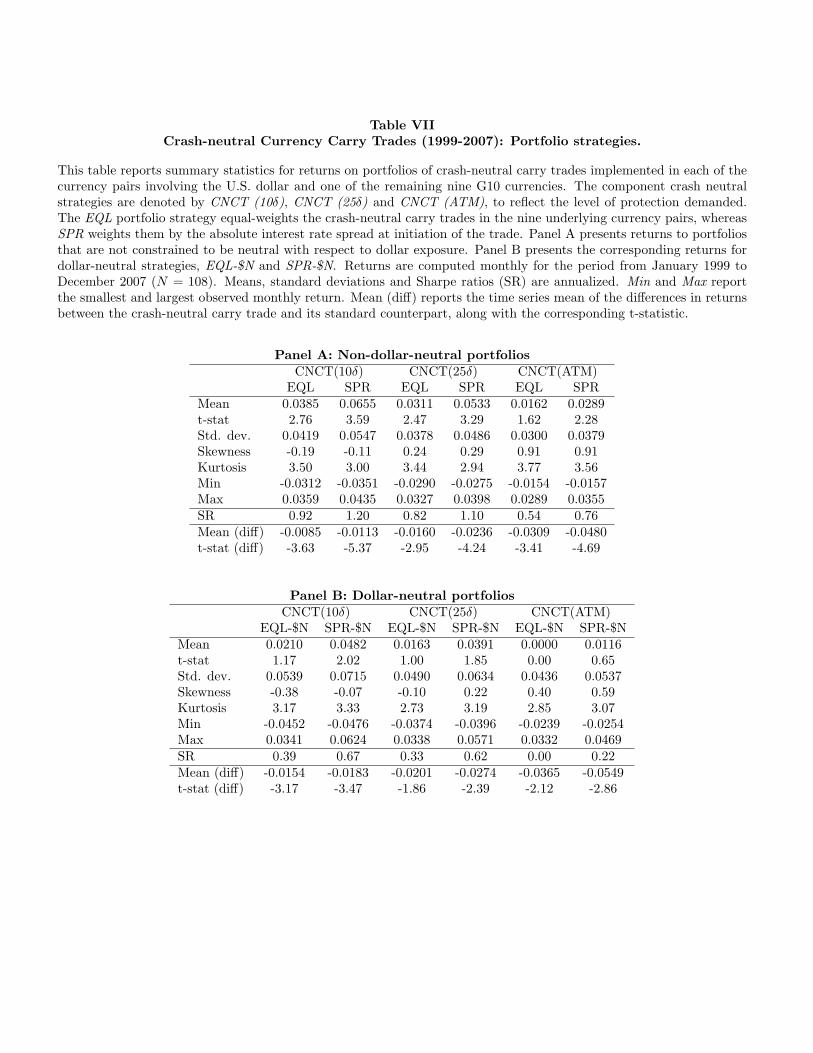
Table VIICrash-neutral Currency Carry Trades (1999-2007): Portfolio strategies.

This table reports summary statistics for returns on portfolios of crash-neutral carry trades implemented in each of thecurrency pairs involving the U.S. dollar and one of the remaining nine G10 currencies. The component crash neutralstrategies are denoted by CNCT (10δ), CNCT (25δ) and CNCT (ATM), to reflect the level of protection demanded.The EQL portfolio strategy equal-weights the crash-neutral carry trades in the nine underlying currency pairs, whereasSPR weights them by the absolute interest rate spread at initiation of the trade. Panel A presents returns to portfoliosthat are not constrained to be neutral with respect to dollar exposure. Panel B presents the corresponding returns fordollar-neutral strategies, EQL-$N and SPR-$N. Returns are computed monthly for the period from January 1999 toDecember 2007 (N = 108). Means, standard deviations and Sharpe ratios (SR) are annualized. Min and Max reportthe smallest and largest observed monthly return. Mean (diff) reports the time series mean of the differences in returnsbetween the crash-neutral carry trade and its standard counterpart, along with the corresponding t-statistic.

Panel A: Non-dollar-neutral portfoliosCNCT(10δ) CNCT(25δ) CNCT(ATM)

EQL SPR EQL SPR EQL SPRMean 0.0385 0.0655 0.0311 0.0533 0.0162 0.0289t-stat 2.76 3.59 2.47 3.29 1.62 2.28Std. dev. 0.0419 0.0547 0.0378 0.0486 0.0300 0.0379Skewness -0.19 -0.11 0.24 0.29 0.91 0.91Kurtosis 3.50 3.00 3.44 2.94 3.77 3.56Min -0.0312 -0.0351 -0.0290 -0.0275 -0.0154 -0.0157Max 0.0359 0.0435 0.0327 0.0398 0.0289 0.0355SR 0.92 1.20 0.82 1.10 0.54 0.76Mean (diff) -0.0085 -0.0113 -0.0160 -0.0236 -0.0309 -0.0480t-stat (diff) -3.63 -5.37 -2.95 -4.24 -3.41 -4.69

Panel B: Dollar-neutral portfoliosCNCT(10δ) CNCT(25δ) CNCT(ATM)

EQL-$N SPR-$N EQL-$N SPR-$N EQL-$N SPR-$NMean 0.0210 0.0482 0.0163 0.0391 0.0000 0.0116t-stat 1.17 2.02 1.00 1.85 0.00 0.65Std. dev. 0.0539 0.0715 0.0490 0.0634 0.0436 0.0537Skewness -0.38 -0.07 -0.10 0.22 0.40 0.59Kurtosis 3.17 3.33 2.73 3.19 2.85 3.07Min -0.0452 -0.0476 -0.0374 -0.0396 -0.0239 -0.0254Max 0.0341 0.0624 0.0338 0.0571 0.0332 0.0469SR 0.39 0.67 0.33 0.62 0.00 0.22Mean (diff) -0.0154 -0.0183 -0.0201 -0.0274 -0.0365 -0.0549t-stat (diff) -3.17 -3.47 -1.86 -2.39 -2.12 -2.86

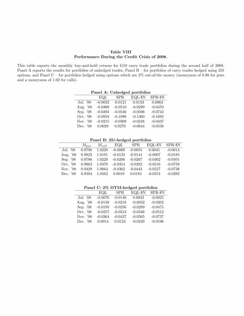
Table VIIIPerformance During the Credit Crisis of 2008.

This table reports the monthly buy-and-hold returns for G10 carry trade portfolios during the second half of 2008.Panel A reports the results for portfolios of unhedged trades, Panel B – for portfolios of carry trades hedged using 25δoptions, and Panel C – for portfolios hedged using options which are 2% out-of-the money (moneyness of 0.98 for putsand a moneyness of 1.02 for calls).

Panel A: Unhedged portfoliosEQL SPR EQL-$N SPR-$N

Jul. ’08 -0.0032 -0.0121 0.0133 0.0063Aug. ’08 -0.0369 -0.0510 -0.0289 -0.0470Sep. ’08 -0.0394 -0.0546 -0.0506 -0.0742Oct. ’08 -0.0958 -0.1098 -0.1360 -0.1695Nov. ’08 -0.0215 -0.0309 -0.0248 -0.0437Dec. ’08 0.0028 0.0270 -0.0644 -0.0556

Panel B: 25δ-hedged portfoliosMput Mcall EQL SPR EQL-$N SPR-$N

Jul. ’08 0.9798 1.0220 -0.0069 -0.0055 0.0045 -0.0014Aug. ’08 0.9823 1.0191 -0.0123 -0.0144 -0.0007 -0.0185Sep. ’08 0.9786 1.0229 -0.0206 -0.0207 -0.0302 -0.0501Oct. ’08 0.9663 1.0378 -0.0354 -0.0282 -0.0516 -0.0759Nov. ’08 0.9429 1.0664 -0.0362 -0.0443 -0.0527 -0.0738Dec. ’08 0.9504 1.0562 0.0019 0.0183 -0.0374 -0.0292

Panel C: 2% OTM-hedged portfoliosEQL SPR EQL-$N SPR-$N

Jul. ’08 -0.0070 -0.0140 0.0033 -0.0025Aug. ’08 -0.0138 -0.0218 -0.0032 -0.0202Sep. ’08 -0.0193 -0.0256 -0.0289 -0.0475Oct. ’08 -0.0257 -0.0313 -0.0346 -0.0512Nov. ’08 -0.0364 -0.0437 -0.0565 -0.0737Dec. ’08 0.0014 0.0123 -0.0249 -0.0196

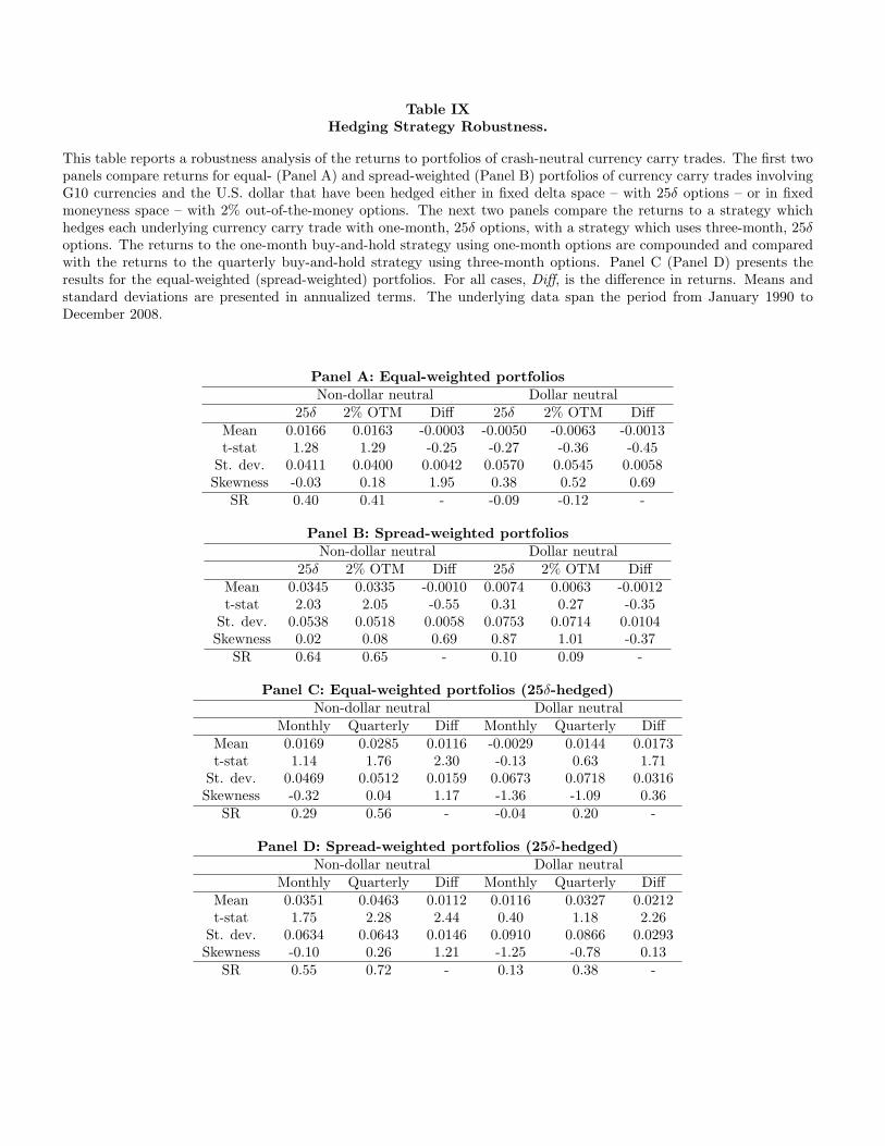
Table IXHedging Strategy Robustness.

This table reports a robustness analysis of the returns to portfolios of crash-neutral currency carry trades. The first twopanels compare returns for equal- (Panel A) and spread-weighted (Panel B) portfolios of currency carry trades involvingG10 currencies and the U.S. dollar that have been hedged either in fixed delta space – with 25δ options – or in fixedmoneyness space – with 2% out-of-the-money options. The next two panels compare the returns to a strategy whichhedges each underlying currency carry trade with one-month, 25δ options, with a strategy which uses three-month, 25δoptions. The returns to the one-month buy-and-hold strategy using one-month options are compounded and comparedwith the returns to the quarterly buy-and-hold strategy using three-month options. Panel C (Panel D) presents theresults for the equal-weighted (spread-weighted) portfolios. For all cases, Diff, is the difference in returns. Means andstandard deviations are presented in annualized terms. The underlying data span the period from January 1990 toDecember 2008.

Panel A: Equal-weighted portfoliosNon-dollar neutral Dollar neutral

25δ 2% OTM Diff 25δ 2% OTM DiffMean 0.0166 0.0163 -0.0003 -0.0050 -0.0063 -0.0013t-stat 1.28 1.29 -0.25 -0.27 -0.36 -0.45

St. dev. 0.0411 0.0400 0.0042 0.0570 0.0545 0.0058Skewness -0.03 0.18 1.95 0.38 0.52 0.69

SR 0.40 0.41 - -0.09 -0.12 -

Panel B: Spread-weighted portfoliosNon-dollar neutral Dollar neutral

25δ 2% OTM Diff 25δ 2% OTM DiffMean 0.0345 0.0335 -0.0010 0.0074 0.0063 -0.0012t-stat 2.03 2.05 -0.55 0.31 0.27 -0.35

St. dev. 0.0538 0.0518 0.0058 0.0753 0.0714 0.0104Skewness 0.02 0.08 0.69 0.87 1.01 -0.37

SR 0.64 0.65 - 0.10 0.09 -

Panel C: Equal-weighted portfolios (25δ-hedged)Non-dollar neutral Dollar neutral

Monthly Quarterly Diff Monthly Quarterly DiffMean 0.0169 0.0285 0.0116 -0.0029 0.0144 0.0173t-stat 1.14 1.76 2.30 -0.13 0.63 1.71

St. dev. 0.0469 0.0512 0.0159 0.0673 0.0718 0.0316Skewness -0.32 0.04 1.17 -1.36 -1.09 0.36

SR 0.29 0.56 - -0.04 0.20 -

Panel D: Spread-weighted portfolios (25δ-hedged)Non-dollar neutral Dollar neutral

Monthly Quarterly Diff Monthly Quarterly DiffMean 0.0351 0.0463 0.0112 0.0116 0.0327 0.0212t-stat 1.75 2.28 2.44 0.40 1.18 2.26

St. dev. 0.0634 0.0643 0.0146 0.0910 0.0866 0.0293Skewness -0.10 0.26 1.21 -1.25 -0.78 0.13

SR 0.55 0.72 - 0.13 0.38 -

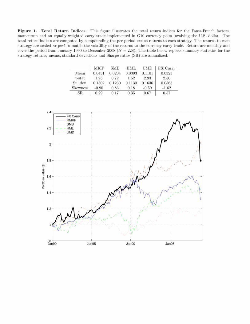
Figure 1. Total Return Indices. This figure illustrates the total return indices for the Fama-French factors,momentum and an equally-weighted carry trade implemented in G10 currency pairs involving the U.S. dollar. Thetotal return indices are computed by compounding the per period excess returns to each strategy. The returns to eachstrategy are scaled ex post to match the volatility of the returns to the currency carry trade. Return are monthly andcover the period from January 1990 to December 2008 (N = 228). The table below reports summary statistics for thestrategy returns; means, standard deviations and Sharpe ratios (SR) are annualized.

MKT SMB HML UMD FX CarryMean 0.0431 0.0204 0.0393 0.1101 0.0323t-stat 1.25 0.72 1.52 2.93 2.50

St. dev. 0.1502 0.1230 0.1130 0.1636 0.0563Skewness -0.90 0.83 0.18 -0.59 -1.62

SR 0.29 0.17 0.35 0.67 0.57

Jan90 Jan95 Jan00 Jan050.8

1

1.2

1.4

1.6

1.8

2

2.2

2.4

Por

tfolio

val

ue (

$)

FX CarryRMRFSMBHMLUMD

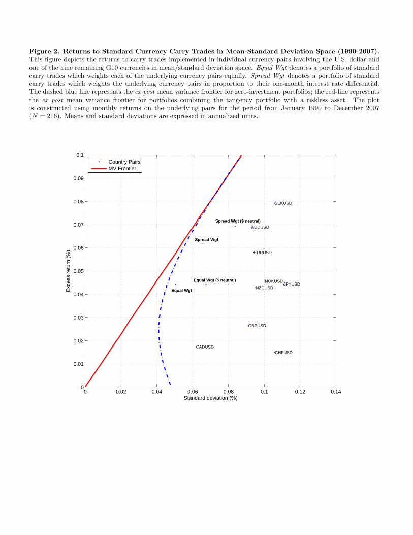
Figure 2. Returns to Standard Currency Carry Trades in Mean-Standard Deviation Space (1990-2007).This figure depicts the returns to carry trades implemented in individual currency pairs involving the U.S. dollar andone of the nine remaining G10 currencies in mean/standard deviation space. Equal Wgt denotes a portfolio of standardcarry trades which weights each of the underlying currency pairs equally. Spread Wgt denotes a portfolio of standardcarry trades which weights the underlying currency pairs in proportion to their one-month interest rate differential.The dashed blue line represents the ex post mean variance frontier for zero-investment portfolios; the red-line representsthe ex post mean variance frontier for portfolios combining the tangency portfolio with a riskless asset. The plotis constructed using monthly returns on the underlying pairs for the period from January 1990 to December 2007(N = 216). Means and standard deviations are expressed in annualized units.

0 0.02 0.04 0.06 0.08 0.1 0.12 0.140

0.01

0.02

0.03

0.04

0.05

0.06

0.07

0.08

0.09

0.1

AUDUSD

CADUSDCHFUSD

EURUSD

GBPUSD

JPYUSDNOKUSD

NZDUSD

SEKUSD

Standard deviation (%)

Exc

ess

retu

rn (

%)

Equal Wgt

Spread Wgt

Equal Wgt ($ neutral)

Spread Wgt ($ neutral)

Country PairsMV Frontier

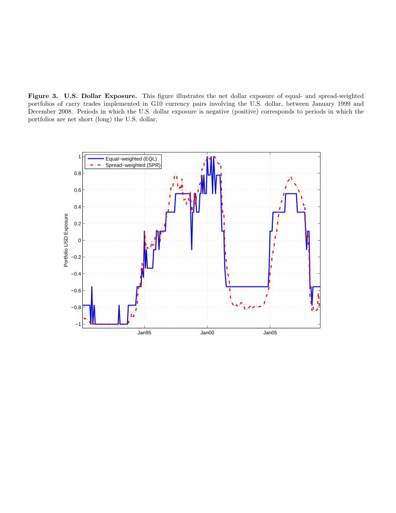
Figure 3. U.S. Dollar Exposure. This figure illustrates the net dollar exposure of equal- and spread-weightedportfolios of carry trades implemented in G10 currency pairs involving the U.S. dollar, between January 1999 andDecember 2008. Periods in which the U.S. dollar exposure is negative (positive) corresponds to periods in which theportfolios are net short (long) the U.S. dollar.

Jan95 Jan00 Jan05

−1

−0.8

−0.6

−0.4

−0.2

0

0.2

0.4

0.6

0.8

1

Por

tfolio

US

D E

xpos

ure

Equal−weighted (EQL)Spread−weighted (SPR)

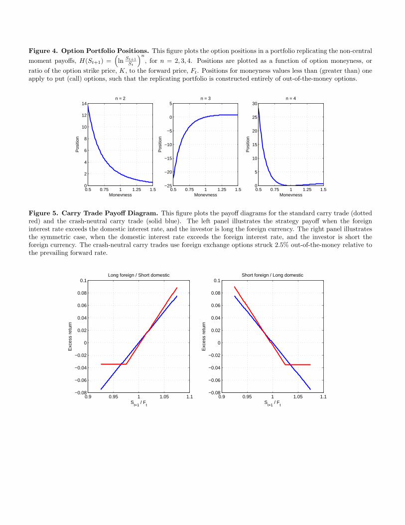
Figure 4. Option Portfolio Positions. This figure plots the option positions in a portfolio replicating the non-centralmoment payoffs, H(St+1) =

(ln St+1

St

)n

, for n = 2, 3, 4. Positions are plotted as a function of option moneyness, orratio of the option strike price, K, to the forward price, Ft. Positions for moneyness values less than (greater than) oneapply to put (call) options, such that the replicating portfolio is constructed entirely of out-of-the-money options.

0.5 0.75 1 1.25 1.50

2

4

6

8

10

12

14n = 2

Moneyness

Pos

ition

0.5 0.75 1 1.25 1.5−25

−20

−15

−10

−5

0

5n = 3

Moneyness

Pos

ition

0.5 0.75 1 1.25 1.50

5

10

15

20

25

30n = 4

Moneyness

Pos

ition

Figure 5. Carry Trade Payoff Diagram. This figure plots the payoff diagrams for the standard carry trade (dottedred) and the crash-neutral carry trade (solid blue). The left panel illustrates the strategy payoff when the foreigninterest rate exceeds the domestic interest rate, and the investor is long the foreign currency. The right panel illustratesthe symmetric case, when the domestic interest rate exceeds the foreign interest rate, and the investor is short theforeign currency. The crash-neutral carry trades use foreign exchange options struck 2.5% out-of-the-money relative tothe prevailing forward rate.

0.9 0.95 1 1.05 1.1−0.08

−0.06

−0.04

−0.02

0

0.02

0.04

0.06

0.08

0.1Long foreign / Short domestic

St+1

/ Ft

Exc

ess

retu

rn

0.9 0.95 1 1.05 1.1−0.08

−0.06

−0.04

−0.02

0

0.02

0.04

0.06

0.08

0.1Short foreign / Long domestic

St+1

/ Ft

Exc

ess

retu

rn

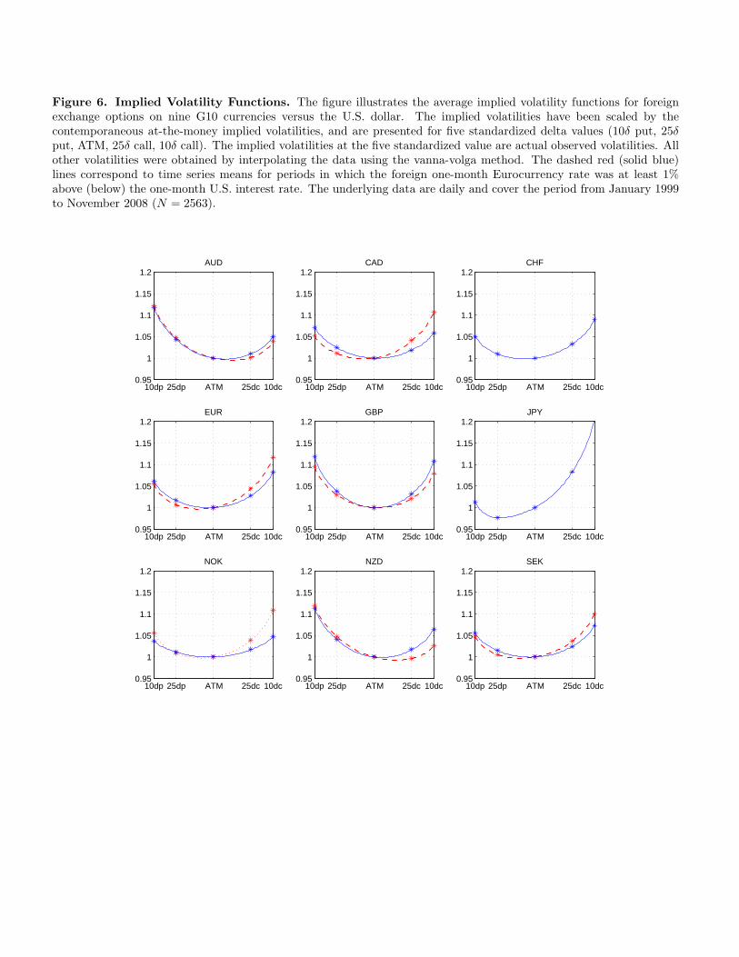
Figure 6. Implied Volatility Functions. The figure illustrates the average implied volatility functions for foreignexchange options on nine G10 currencies versus the U.S. dollar. The implied volatilities have been scaled by thecontemporaneous at-the-money implied volatilities, and are presented for five standardized delta values (10δ put, 25δput, ATM, 25δ call, 10δ call). The implied volatilities at the five standardized value are actual observed volatilities. Allother volatilities were obtained by interpolating the data using the vanna-volga method. The dashed red (solid blue)lines correspond to time series means for periods in which the foreign one-month Eurocurrency rate was at least 1%above (below) the one-month U.S. interest rate. The underlying data are daily and cover the period from January 1999to November 2008 (N = 2563).

10dp 25dp ATM 25dc 10dc0.95

1

1.05

1.1

1.15

1.2AUD

10dp 25dp ATM 25dc 10dc0.95

1

1.05

1.1

1.15

1.2CAD

10dp 25dp ATM 25dc 10dc0.95

1

1.05

1.1

1.15

1.2CHF

10dp 25dp ATM 25dc 10dc0.95

1

1.05

1.1

1.15

1.2EUR

10dp 25dp ATM 25dc 10dc0.95

1

1.05

1.1

1.15

1.2GBP

10dp 25dp ATM 25dc 10dc0.95

1

1.05

1.1

1.15

1.2JPY

10dp 25dp ATM 25dc 10dc0.95

1

1.05

1.1

1.15

1.2NOK

10dp 25dp ATM 25dc 10dc0.95

1

1.05

1.1

1.15

1.2NZD

10dp 25dp ATM 25dc 10dc0.95

1

1.05

1.1

1.15

1.2SEK

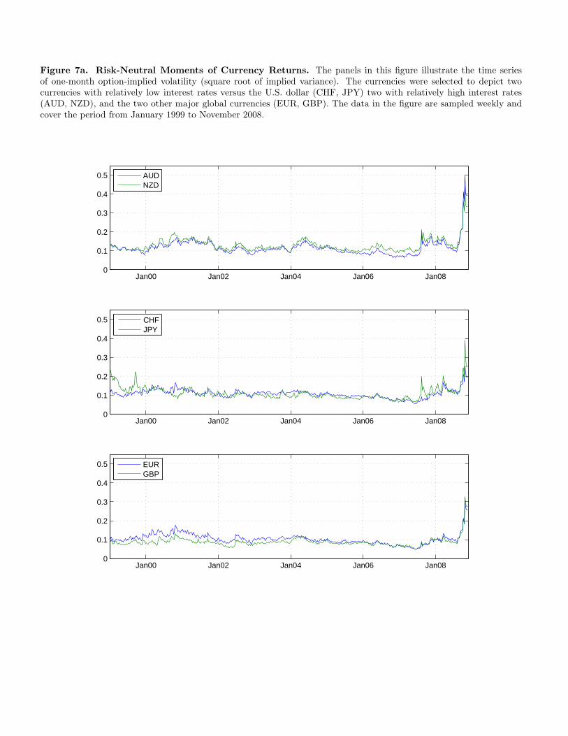
Figure 7a. Risk-Neutral Moments of Currency Returns. The panels in this figure illustrate the time seriesof one-month option-implied volatility (square root of implied variance). The currencies were selected to depict twocurrencies with relatively low interest rates versus the U.S. dollar (CHF, JPY) two with relatively high interest rates(AUD, NZD), and the two other major global currencies (EUR, GBP). The data in the figure are sampled weekly andcover the period from January 1999 to November 2008.

Jan00 Jan02 Jan04 Jan06 Jan080

0.1

0.2

0.3

0.4

0.5

AUDNZD

Jan00 Jan02 Jan04 Jan06 Jan080

0.1

0.2

0.3

0.4

0.5

CHFJPY

Jan00 Jan02 Jan04 Jan06 Jan080

0.1

0.2

0.3

0.4

0.5

EURGBP

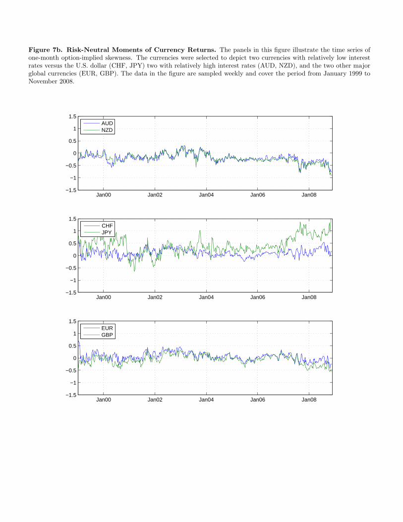
Figure 7b. Risk-Neutral Moments of Currency Returns. The panels in this figure illustrate the time series ofone-month option-implied skewness. The currencies were selected to depict two currencies with relatively low interestrates versus the U.S. dollar (CHF, JPY) two with relatively high interest rates (AUD, NZD), and the two other majorglobal currencies (EUR, GBP). The data in the figure are sampled weekly and cover the period from January 1999 toNovember 2008.

Jan00 Jan02 Jan04 Jan06 Jan08−1.5

−1

−0.5

0

0.5

1

1.5

AUDNZD

Jan00 Jan02 Jan04 Jan06 Jan08−1.5

−1

−0.5

0

0.5

1

1.5

CHFJPY

Jan00 Jan02 Jan04 Jan06 Jan08−1.5

−1

−0.5

0

0.5

1

1.5

EURGBP

Figure 8. Crash-neutral Currency Carry Trade Strategy Returns. The figure depicts the total returnindices for the standard carry trade and crash-neutral carry trades with various degrees of downside protection. Thestrategy returns are an spread-weighted combination of the carry trade returns for nine G10 currency pairs involv-ing the U.S. dollar. Returns are computed monthly and cover the period from January 1999 to December 2008 (N = 120).

Jan00 Jan02 Jan04 Jan06 Jan08

1

1.2

1.4

1.6

1.8

2

2.2

UnhedgedCrash−neutral (10δ)Crash−neutral (25δ)Crash−neutral (ATM)