creation “the tale of three crystal lattice structures
TRANSCRIPT
CREATION “The Tale of Three Crystal Lattice Structures” VOLUME II
Copyright © 2019 by Thomas McKernon. All rights reserved. © 1-8185354701 TX 8-817-930 ‘Fair Use Notice’: This Paper contains a few figures, photos, images, illustrations and text citations from other journals, books, magazines and public domains the use of which in most instances has been specifically authorized by the copyright owner for academic and non-profit usages. As such, materials with proper citation and acknowledgement are included for the purpose of scientific research, comments, and criticism in an effort to advance our understanding of Nature and the Universe. The material usage of which constitutes a ‘fair dealing’ and fair use’ of any copyrighted material as provided for in U.S. Copyright Law, 15 U.S.C. Section 1051(b) and Canada Copyright Law Part III Section 29.
The Context presented: the Theoretical ideas and premises, Applications, Derivations, Expressions and Conclusions not encompassed by the above “Fair Use” clause, are the Original ideas and compilation by Thomas McKernon, all rights, authorship and copyright belong to Thomas McKernon, Physics by Tom™; ©https://physicsbytom.com/ October 11, 2019. All References are listed in the References Section of the Website; and all Calculations, Derivations, Photos, Graphics, Illustrations and Figures.
VOLUME II In this Volume the Equations, Derivations, and interactions between the four Major Tensors are presented and discussed along with any possible conclusions applicable and following along the same approach as Volume I. These Derivations and Calculations are related to the Longitudinal Plane Waves, whereas, Volume I was directed at the Transient Plane Waves.
It must be remembered that the analysis is based upon using the Cartenoid and Helicoid structures to mathematically model the four major field tensors: Dielectric, Electric, Magnetic and Gravitational Tensors. The Cartenoid models the Torsional Double-hyper-trochoid structure of the EM fields, while the Helicoid models the twisting of these forces in Centripetal and Centrifugal contractions and expansions. The combined parameterized vectors allow for the mathematical modeling using Cartan Geometry to derive the associated Euler-Lagrangian equations and the Tetrad expressions of the Hamiltonians. The resultant expressions may be interpreted as Annihilation/ creation events associated with elemental periodic atoms, excited atomic ions, photons, positrons, and other associated results.
Why is the Cartenoid chosen and what or where does the premise originate? It just so happens that our Sun as the center of our solar system does not orbit in a perfect circle. Our Sun orbits in an epitrochoid motion as a result of gravitational and electromagnetic forces from the orbiting planets (such as Mercury, Venus, Earth and Mars). The Sun’s orbit and solar activity affects other planets and moons with its epitrochoid (Cartenoid) motion. [155] More discussions related to the Sun’s effect upon the Earth’s magnetosphere and ionisphere will be discussed in later volumes.
The Helicoid is used in modeling and originates from the intra-nucleonic dynamics of the two up quarks and one down quark in the proton of the Hydrogen atom. These dynamics create a twisted torsional motion which dictates the shape of all things in the universe from our human DNA to Magnetic quasars emissions. It is also interesting that solar plasma ejections and solar coronal mass ejections interact with the Earth’s magnetosphere causing interferences and blackouts of electrical grids. Such was the case on midnight of 22 September 2009 when a solar storm released highly energetic plasma that caused a colorful display of aurora as far south as New York city and within a few minutes caused the entire eastern half of the U.S. without power. These solar plasma releases travel through the interspace between the sun and earth at varying speeds but always with a helical pattern that when impacts the Earth’s magnetosphere at the correct incident angle can cause havoc to the electrical power grid by infusing a DC into the AC power lines which overloads transformers on the grid. This type of overload occurred in Canada in March of 1989 when a solar storm caused a disruption of Hydro-Quebec power lines and resulted in a blackout affecting six million people. [155] The Carrington Event of 1859 originated from a Solar Plasma Event which sent a plasma cloud towards the earth at 2,380 Km/sec. which hit the earth about 17 seconds later. The Solar event combined the energies of a solar proton event and a CME resulting in magnificent aurora and melting of some telegraph lines. From magnetometer readings and observation of the sun’s surface, the emission point was close to 50 million degrees Celsius. [155] The Helicoid is formed as a result of the interactions between the Magnetic Spatial Centrifugal inertia and the Dielectric Counter-Space Centripetal inertial forces along the Dielectric plane. This interaction forms the spirals (Landau-Zener) toward and from the dielectric plane in the necessity to conserve angular momentum.
“Plasmas pervade intergalactic, interstellar space, interplanetary space, and the space environments of planets” [161]
Later in Volume II, the application of the theory is discussed regarding LENR (Cold Fusion) reactor, advanced propulsion technology, bending the curvature of Spacetime, and organic cell structure, medicine, as well as, cosmology.
ADDENDUM I Derivation of the Longitudinal Planar Wave Propagation Expression Starting with the Combined Parameterized Vectoral Equation:
𝑿(𝒖, 𝒗) = {[(𝟐𝟓𝝅𝟒
𝟒𝟕) ∗ [( 𝟓𝝅
𝟏𝟗𝟐) − 𝒗𝟐)] + 𝒗 ∗ (𝟏 − 𝒖𝟐
𝟐 )]; (𝟐𝟕 − 𝒗); 𝟎]} And substituting the Edge Length for the Dodecahedron, (5*Φ) gives:
𝑿(𝒖, 𝒗) = {[(𝟐𝝅𝟑) ∗ 𝜱𝒗 ∗ 𝜱𝒖𝟐 − [𝜱𝒗
𝟐 − ( 𝟏𝟐𝟓𝟗) ∗ 𝜱𝒗 + 𝟑
𝟓]; [𝟓 ∗ ((𝟔𝝅𝟐
𝟏𝟏) + 𝜱𝒗)]; 𝟎]}
Taking the Partial derivative with respect to (u, β) gives:
𝑿𝜷 = {[((𝟒𝝅𝟑) ∗ 𝜱𝓔 ∗ 𝜱𝜷); 𝟎; 𝟎] and,
𝑿𝓔 = {[[(𝟐𝝅𝟑) ∗ 𝜱𝜷𝟐 − 𝟐 ∗ 𝜱𝓔 − ( 𝟏
𝟐𝟓𝟗)]; +𝟓; 𝟎]}
And, (I) 𝜱𝜷⨂𝜱𝓔 = [𝟎; 𝟎; 𝟐𝟎 ∗ 𝝅𝟑 ∗ 𝜱𝜷 ∗ 𝜱𝓔]
This is interpreted as the Longitudinal Propagating Plane Wave; ψ, which takes the form of a Hankel Transform Equation. And the 𝜱𝜷 and𝜱𝓔 Terms can be expressed as Cosmic Equation States related to the Permittivity and Permeability of the Vacuum, respectively.
Therefore, (I) above takes the form: 𝝍(𝝆) = 𝜴 ∗(𝑰);
𝑾𝒉𝒆𝒓𝒆𝜴 = [(𝟓 ∗ 𝜶 ∗ ( 𝝐𝝐𝟎) ∗ ( 𝝁
𝝁𝟎))]𝒘𝒉𝒊𝒄𝒉𝒆𝒒𝒖𝒂𝒕𝒆𝒔𝒕𝒐:
𝜴 = [L𝟓 ∗ 𝟕. 𝟐𝟗𝟕𝟑𝟓𝟐𝟓L𝟏𝟎0𝟑P ∗ 𝟔. 𝟕𝟖L𝟏𝟎𝟓P ∗ (. 𝟗𝟗𝟗𝟓𝟓)S = 𝟐. 𝟒𝟕𝟐𝟔𝟗(𝟏𝟎𝟒) and ψ takes the form: 𝝍𝒏(𝒓) ≈ 𝑯𝒏(𝒇(𝒕)) = 𝜴 ∗ ∫ 𝒕 ∗ 𝑱𝒏(𝝓, 𝒕) ∗ 𝒇(𝒕)𝒅𝒕
2𝟎 And,
𝒈(𝒒) = 𝟐𝝅 ∗ ∫ 𝒇(𝒓) ∗ 𝑱𝟎(𝟐𝝅𝒒𝒓) ∗ 𝒓 ∗ 𝒅𝒓
2𝟎 where 𝒇(𝒓) = ∫ 𝑯𝝂(𝒌) ∗ 𝑱𝝂(𝒌𝒓) ∗ 𝒌 ∗ 𝒅𝒌
2𝟎 𝒂𝒏𝒅;
𝑯𝝂(𝒌) = ∫ 𝒇(𝒓) ∗ 𝑱𝝂(𝒌𝒓) ∗ 𝒓 ∗ 𝒅𝒓
2𝟎 𝒂𝒏𝒅𝒇(𝒓) = 𝟐𝝅 ∗ ∫ 𝒈(𝒒) ∗ 𝑱𝟎(𝟐𝝅𝒒𝒓) ∗ 𝒒 ∗ 𝒅𝒒
2𝟎
J0(r) are Bessel Functions of Zero Order. It is worth noting that the Longitudinal Planar wave has components related to the Dielectric, Electric, and Magnetic Field Tensors and probably the Gravitational Tensor. The Components also have Transient components which at least for the Dielectric (LD) wave propagation is short-lived and has a low power density. Tesla tried to promote electrical power distribution by means of gathering ionic power from the atmosphere and transmitting it through the ground. A modern-day pilot project exists in Redwood, Texas which is promoting the similar concept to change Electrical power distribution from the aged Power Lines to distribution from major sub-stations to step-down transformer sub-stations thus alleviating the aging effects, (Age and Load growth) on the cross-country power lines. See [31]
Contrary to the Transverse waves studied in the prior volume, Longitudinal Waves were first named ‘Tesla’ waves after their discoverer Nikolai Tesla when he operated his monopole magnifying transmitter tower. Unlike Transverse waves described by Maxwell as the conventional electromagnetic force field wave, longitudinal waves propagate with field gradients aligned only parallel to the direction of wave motion. The longitudinal waves may be expressed by representing the electrostatic potential equations in terms of retarded time assuming the LW propagates through the dielectric vacuum at some finite velocity, υ, which may be greater than the speed of light. The LW is expressed by:
𝜵𝟐𝝋(𝒓, 𝒕) = 𝟏
𝝊𝟐∗ 𝝏
𝟐𝝋𝝏𝒕𝟐 Such LWs have been produced and received by such researchers as T. Townsend
Brown, Bedini, and Russian physicists E. Podkletnov and G. Modanese. The two latter Russian physicists produced a Gravity wave beam by discharging 2 Megavolt electron pulse from a 10 cm diameter superconducting ceramic disc. The electric field is reinforced magnetic field and assists in collimating the discharge and helps to propagate forward a coherent planar wave. These pulsed Gravity waves were found to accelerate masses with an instantaneous repulsive force up to 1000 g’s even at a distance of 150 meters. Further information was reported by author, Nick Cook, in Jane’s Defense Weekly, 2002. In his article, Cook reported that a Russian laboratory demonstrated that the Gravity beam was able to repel one km away and exhibits negligible power loss at distances up to 200 km away. [86]

Addendum II Derivation of the Gaussian 1st Fundamental Forms and the Euler-Lagrangian Equations related to the interactions of the Electric-Magnetic Tensors
Like Volume II, we start with the Combined Cartenoid and Helicoid Parameterized Vector modeled in the same approach used in Volume I, (i.e., the Cubic Crystal Lattice Structure in the Affine Complex Phase Plane).
The Combined Parameterized Vector is:
𝑿(𝒖, 𝒗) = {[[(𝟐𝟓𝝅𝟒
𝟒𝟕) ∗ (( 𝟓𝝅𝟏𝟗𝟐) − 𝒗
𝟐) + 𝒗 ∗ (𝟏 − 𝒖𝟐
𝟐 )];[𝟐𝟕 ∗ 𝒗]; 𝟎]} From which the Partial derivatives related to u and v are taken resulting in :
𝑿𝒖 = {[𝒗 ∗ (𝟏 − 𝒖)]; 𝟎; 𝟎]}𝑨𝒏𝒅𝑿𝒗 = {[(𝟓𝟎𝝅𝟒
𝟒𝟕) ∗ 𝒗 +(𝟏 − 𝒖𝟐
𝟐 )];(−𝟏); 𝟎]}
Using these base equations, the Gaussian 1st Fundamental Form Factors are Derived:
𝑰.𝑬𝟏𝑹 = {[𝒗𝟐 − 𝟐 ∗ 𝒖 ∗ 𝒗𝟐 + 𝒖𝟐 ∗ 𝒗𝟐]} 𝑰𝑰.𝑭𝟏𝑹 = {[(𝟏𝟎𝝅
𝟓
𝟐𝟕) ∗ 𝒗 ∗ [𝒖 ∗ (𝒗 − ( 𝟒
𝟖𝟐𝟗) ∗ 𝒖 − 𝒗]]} And,
𝑰𝑰𝑰.𝑮𝟏𝑹 = {[( 𝟓𝟑𝟔𝟗) ∗ 𝜶 ∗ 𝒓𝒎𝒔′ ∗ 𝒄 ∗ (𝒏𝝅) ∗ 𝑮 ∗ 𝑺𝒆 ∗ (
𝝌𝒏)] ∗ [𝒗𝟐 − ( 𝟏𝟓𝟎) ∗ (𝟏 −
𝒖𝟐
𝟐 ) ∗ 𝒗]}
From these expressions, the Euler-Lagrangian Equations Left-Hand-Sides (LHS) are Derived: (𝑰𝑽. 𝟏)𝟏𝒔𝒕𝑬 − 𝑳𝑬𝒒𝒏. 𝑳𝑯𝑺: = 𝝏
𝝏𝒕[[𝑬𝟏𝑹] ∗ �̇� +[𝑭𝟏𝑹] ∗ 𝒗] =
= {[ 𝝏
𝝏𝒕[𝑬𝟏𝑹] ∗ �̇� + [𝑬𝟏𝑹] ∗ �̈� + 𝝏
𝝏𝒕[𝑭𝟏𝑹] ∗ �̇� + [𝑭𝟏𝑹] ∗ �̈�]}
(𝑰𝑽. 𝟏)𝟏𝒔𝒕𝑬 − 𝑳𝑬𝒒𝒏. 𝑳𝑯𝑺 = {(𝟕𝝅
𝟏𝟎) ∗ [[�̇�𝜷|𝜱𝜷|�̇�𝓔 + (𝟏𝟐) ∗ �̇�𝜷|𝜱𝓔
𝟐] + (𝟏𝟒) ∗ [�̇�𝜷|�̇�𝓔(𝟏 + (𝟏𝟐) ∗ 𝜱𝜷
𝟐)]] −(𝝅
𝟐) ∗ [(𝟏 − (𝟏𝟐) ∗ 𝜱𝜷)|{𝜱𝜷
𝟐 , �̈�𝜷}}
+{[𝟖𝟒 ∗ 𝝅𝟐 ∗ �̇�𝓔|(�̇�𝜷 − ( 𝟏𝟏𝟎𝟎) ∗ �̇�𝓔) + (𝟓𝟔) ∗ �̇�𝜷|�̇�𝓔 + (𝟓𝟗) ∗ �̇�𝓔|[�̇�𝓔 + (𝟏𝟐) ∗ �̇�𝜷 ∗ 𝜱𝓔] + (
𝟖𝝅𝟓
𝟑) ∗ (𝜱𝜷 − 𝟐 ∗ �̇�𝓔) +𝟒𝟗 ∗ �̇�𝓔
𝟐 +[(𝟑𝝅
𝟑
𝟒) ∗ [(𝟏 − ( 𝟏
𝟐𝟎𝟎) ∗ 𝜱𝜷 ∗ 𝜱𝓔 −𝜱𝜷𝟐 ∗ (𝟏 − (𝟏𝟐) ∗ 𝜱𝜷)]]|{�̈�𝓔, 𝜱𝓔
𝟐} Taking the Partial Derivative with respect to β results in:
(𝑰𝑽. 𝟏. 𝟏) 𝝏𝝏𝜷= {(𝟓𝝅
𝟗) ∗ {{�̇�𝜷
𝝁 , �̇�𝓔};𝜱𝜷} + (𝟕𝝅𝟏𝟎) ∗ {{�̇�𝜷, �̇�𝓔};𝜱𝜷
𝝁} + (𝟓𝝅𝟗) ∗ [{{𝜱𝜷, �̈�𝜷};𝜱𝜷
𝝁 − (𝟓𝝅𝟗){{�̈�𝜷, 𝜱𝜷
𝝁}; �̇�𝜷}
+(𝟑𝝅𝟓
𝟒) ∗ {{�̇�𝓔, 𝜱𝓔}; �̇�𝜷
𝝁} + (𝟓𝝅𝟓
𝟏𝟏) ∗ [�̇�𝓔|�̇�𝜷
𝝁] + (𝟏𝟎𝝅𝟓𝟕) ∗ [�̇�𝜷|�̇�𝓔] + (
𝟓𝝅𝟗) ∗ [𝜱𝜷
𝝁|{𝜱𝜷𝟐 , �̈�𝜷}]

+(𝟓𝝅𝟗) ∗ [𝜱𝜷|{𝜱𝜷
𝟐 , �̈�𝜷𝝁}] + [(𝟑𝝅
𝟏𝟐
𝟒) ∗ 𝜱𝜷
𝝁] + (𝟏𝟎𝝅𝟓𝟕) ∗ [{𝓗1,𝜵𝜱3 𝓔}|𝜵𝜱𝜷]𝑾𝒉𝒆𝒓𝒆𝓗1𝒊𝒔𝒂[𝟑𝒙𝟏]𝑴𝒂𝒕𝒓𝒊𝒙𝒆𝒒𝒖𝒊𝒗𝒂𝒍𝒆𝒏𝒕𝒕𝒐:
𝓗Q=
⎩⎨
⎧[{𝜱U𝜷𝒚𝝁 , �̇�𝜷𝒛}]}
[{𝜱U𝜷𝒛𝝁 , �̇�𝜷𝒙}]}
[{𝜱U𝜷𝒚𝝁 , �̇�𝜷𝒙}]}
Now taking the Partial Derivative with respect to ε produces:
(𝑰𝑽. 𝟏. 𝟐) 𝝏𝝏𝜺= {(𝟕𝝅
𝟏𝟎) ∗ {{�̇�𝜷, �̇�𝓔
𝝐 };𝜱𝜷} + (𝟕𝝅𝟏𝟎) ∗ {{�̇�𝜷, 𝜱𝓔
𝝐 },𝜱𝓔} − (𝟑𝟏𝝅𝟑𝟔) ∗ [�̇�𝜷|�̇�𝓔
𝝐 ] − (𝝅𝟑
𝟐) ∗ [�̇�𝓔|�̇�𝓔
𝝐 ]
+{( 𝟓𝟏𝟖) ∗ [{�̇�𝓔
𝝐 , 𝜱𝓔} + {�̇�𝓔, 𝜱𝓔𝝐 }]|�̇�𝜷} − [(
𝟏𝟔𝝅𝟓
𝟑) ∗ �̇�𝓔
𝝐 ] + {(𝟑𝝅𝟒) ∗ [[�̇�𝓔|�̇�𝓔𝝐 ]|{�̈�𝓔, 𝜱𝓔
𝟐}]}
−{(𝟏𝟓𝟒𝟑) ∗ [[𝜱𝜷|𝜱𝓔
𝝐 ]|{�̈�𝓔, 𝜱𝓔𝟐}}}
(𝑰𝑽. 𝟐)𝟐𝒅𝑬 − 𝑳𝑬𝒒𝒏. 𝑳𝑯𝑺: = 𝝏
𝝏𝒕[[𝑭𝟏𝑹] ∗ �̇� + [𝑮𝟏𝑹] ∗ �̇�] =
= {[ 𝝏
𝝏𝒕[𝑭𝟏𝑹] ∗ �̇� + [𝑭𝟏𝑹] ∗ �̈� + 𝝏
𝝏𝒕[𝑮𝟏𝑹] ∗ �̇� + [𝑮𝟏𝑹] ∗ �̈�]}
(𝑰𝑽. 𝟐)𝟐𝒅𝑬 − 𝑳𝑬𝒒𝒏. 𝑳𝑯𝑺 = [(𝟓𝟐) ∗ 𝜶 ∗ 𝒓𝒎𝒔′ ∗ 𝒄 ∗ (𝒏𝝅) ∗ 𝑮 ∗ 𝑺𝒆 ∗ 𝒈𝒆 ∗ (
𝝌𝒏)] ∗ {[{{�̈�𝓔, 𝜱𝓔
𝟒};𝜱𝜷𝟐}
+{{𝜱𝓔𝟒, 𝜱𝜷
𝟐}; �̈�𝓔} +( 𝟐𝟐𝟓) ∗ {𝜱𝓔𝟐, 𝜱𝜷}]}
The 2d E-L Eqn. LHS is easier to work with.
Now taking the Partial Derivatives with respect to (u, β) and (v, ε) produces the two ‘Tetrad’ Matrices: (IV.2.1) 𝝏
𝝏𝜷≈ {[(𝟏
𝟑) ∗ 𝜶 ∗ 𝒓𝒎𝒔′ ∗ 𝒄 ∗ (𝒏𝝅) ∗ 𝑹𝒄 ∗ 𝑺𝒆 ∗ 𝒈𝒆 ∗ (
𝝌𝟑)] ∗ [{�̈�𝓔, 𝜱𝓔}|{𝜱𝓔
𝟐, 𝜱𝜷𝝁}]}
(IV.2.2) 𝝏
𝝏𝓔≈ {[(𝟏
𝟓) ∗ 𝜶 ∗ 𝒓𝒎𝒔′ ∗ 𝒄 ∗ (𝒏𝝅) ∗ 𝑹𝒄 ∗ 𝑺𝒆 ∗ 𝒈𝒆 ∗ (
𝝌𝟐)] ∗ [[{�̈�𝓔
𝝐 , 𝜱𝓔𝟐} +( 𝟑𝟖𝟓) ∗ {𝜱𝓔
𝟐, 𝜱𝓔𝝐 }]|𝜱𝜷]}
Comparing IV.1.1 and IV.1.2 with IV.2.1 and IV.2.2, it is obvious that using the IV.2.1 and IV.2.2 is much more convenient and contains the same information due to Isometry.
Therefore the “Tetrad” Matrix is:
"𝑻𝒆𝒕𝒓𝒂𝒅" ≈ 𝜴𝟏𝜴𝟐^[{�̈�𝓔, 𝜱𝓔}|{𝜱𝓔
𝟐, 𝜱𝜷𝝁}] 𝟎
𝟎 [[{�̈�𝓔𝝐 , 𝜱𝓔
𝟐} + ( 𝟑𝟖𝟓) ∗ {𝜱𝓔𝟐, 𝜱𝓔
𝝐 }]|𝜱𝜷]]_
Where 𝜴𝟏 ≈ [(𝟏𝟓) ∗ 𝜶 ∗ 𝒓𝒎𝒔′ ∗ 𝒄 ∗ (𝒏𝝅) ∗ 𝑹𝒄 ∗ 𝑺𝒆 ∗ 𝒈𝒆 ∗ (𝝌𝒏)]
And, 𝜴𝟐 ≈ [(
𝟏𝟑) ∗ 𝜶 ∗ 𝒓𝒎𝒔′ ∗ 𝒄 ∗ (𝒏𝝅) ∗ 𝑹𝒄 ∗ 𝑺𝒆 ∗ 𝒈𝒆 ∗ (
𝝌𝟑)] And,
(𝑨)∆𝑬 ≈ a 𝟏𝟐𝟖b ∗ cde𝜱𝓔
𝟐, 𝜱𝓔𝝐 fg𝜱𝜷 + (𝟗𝝅) ∗ e�̈�𝓔
𝝐 , 𝜱𝓔𝟐fi − je�̈�𝓔, 𝜱𝓔fk c𝜱𝓔
𝟐, 𝜱𝜷𝝁lml
As an example, the 2d Term is comprised of Electron acceleration and Electron Angular Momentum; and represents an Electron Annihilation event creating a Photon(s).
𝜱𝓔𝟐 = 𝟗. 𝟏𝟎𝟗𝟑𝟗𝟎(𝟏𝟎:𝟑𝟏)𝒌𝒈 ∗ 𝟑. 𝟖𝟔𝟏𝟔(𝟏𝟎:𝟏𝟑)𝒎 ∗ 𝟐. 𝟏𝟖𝟕𝟕(𝟏𝟎𝟔)𝒎𝒔 which is equal to: 𝟒. 𝟖𝟎𝟑𝟔(𝟏𝟎:𝟐𝟎)𝒆𝑽.
𝑨𝒏𝒅�̈�𝓔
𝝐 𝒊𝒔𝒕𝒉𝒆𝒂𝒅𝒋𝒖𝒔𝒕𝒆𝒅𝑶𝒑𝒕𝒊𝒎𝒂𝒍𝑬𝒍𝒆𝒄𝒕𝒓𝒐𝒏𝒂𝒄𝒄𝒆𝒍𝒆𝒓𝒂𝒕𝒊𝒐𝒏 for (CL) Lattice Creation. The total term yields the “Event Energy” which is the energy at the Landau-Zener zero-line equivalent to: 𝑬𝒏𝒆𝒓𝒈𝒚𝒐𝒇𝑬𝒍𝒆𝒄𝒕𝒓𝒐𝒏𝑨𝒏𝒏𝒊𝒉𝒊𝒍𝒂𝒕𝒊𝒐𝒏𝒄𝒓𝒆𝒂𝒕𝒊𝒏𝒈𝑷𝒉𝒐𝒕𝒐𝒏(𝒔):𝑬𝑨𝑷𝒉 ≈ 𝟔𝟏𝒆𝑽.It is also noted that above the Landau-Zener Zero-line, the Energy dissipates quickly whereas below the line, the energy increases in concentration. Each level is a sub-harmonic of the Golden frequency or various octaves. The Electro-Magnetic spectrum spans a range from wavelengths of (𝟏𝟎:𝟏𝟔) meters to (𝟏𝟎𝟖) meters which is a range of doublings (𝟐𝟕𝟑) or 73 octaves. This is the spectrum of Nature’s music. [113] The above Energy level is equivalent to about 1.5 (𝟏𝟎𝟏𝟔)Hz.
Energy is stored in atomic bonds (inside atom’s nucleus); in ionic and covalent bonding, as well as, Hydrogen bonds which come to be by dipole interactions between molecules. In the latter case, Hydrogen is bonded to an electro-negative atom such as oxygen or nitrogen. As a result, the center of gravity is shifted closer to the other atom than it is to the Hydrogen atom which leaves a net positive charge allowing further bonding onto the non-bonded side of the hydrogen atom for added bonding to other electro-negative atoms. If one looks at the human DNA helix it is seen as anti-symmetrical (out of phase) RNA linked dipole helixes. The hydrogen bonds between the base pairs in the DNA double helix are responsible for the template mechanism which ensures accurate reproduction of the DNA molecule during replication. Hydrogen bonds are also used to stabilize the α-helical secondary structure of polypeptide chains and β-pleated sheet structures between polypeptide chains. As an example, hydrogen has a dipole moment of 1.85 Debye, (1Debye equals to: 𝟑. 𝟑𝟖(𝟏𝟎:𝟑𝟎)𝑪𝒐𝒖𝒍𝒐𝒎𝒃𝒎𝒆𝒕𝒓𝒆. Polypeptide chains in a α-helical structure contain 500 Debye because the dipole moments are all aligned in the same direction. However, in the double helical DNA structure the dipole moments oppose each other which means there is zero net dipole moment. It is also noted that such dipole moments in the spinal column align in the same direction, which are due to sugar-phosphate bonds. The most significant bonds are between hydrogen bonds in water molecules forming dynamic clusters or aggregates with lifetimes between𝟏𝟎:𝟏𝟏𝒕𝒐𝟏𝟎:𝟏𝟎𝒔𝒆𝒄. Water makes up 70-80% of all living organisms. [120] Energy, entropy, information and organization appear to be interconnected as in information related to energy/ entropy flow and storage depots.
Another important aspect is the timing at which Energy can be transferred. In typical conditions this is bounded by the speed of light. Light refracted in water travels slower while in living organism’s energy is transferred via chemical processes. An example is the conversion of a photon of light striking the retina of the eye. In this case, the photon is absorbed into a molecule rhodopsin which is the visual pigment in special membrane stacks in the outer portion of the rod-cell. This impingement results in a nerve impulse signal coming out of the opposite end of the rod-cell whose energy is a million times the energy contained in the original photon. This effect is well understood as the ‘molecular cascade’ of reactions in which the first receptor protein actuates many more molecules in the second protein transducing which then activates a molecule of phosphodiesterase in order to split many molecules of guanosine monophosphate, cGMP. The molecules of cGMP keep sodium ion channels open. As a result, the sodium channels giving a rise to an increased electrical polarization of the cell membrane from -40 mV to -70 mV which is enough to cause nerve impulse.
This transfer of energy occurs in about 𝟏𝟎:𝟏𝟒seconds. [120]. Organisms are amazing things in a position to produce cycles which are negentropic, (i.e., stored energy, ∆𝑺 = 𝟎). This stored energy can be used for work applications in many different modes.
The 1st & 3d Terms in (A) above are Electron Capture events by a Proton creating Hydrogen atoms.
Next, by solving for the Determinant 𝓓𝓗: 𝓓"𝓗 ≈ {[(𝟏𝟓) ∗ 𝜶 ∗ 𝒓𝒎𝒔′ ∗ 𝒄 ∗ 𝑹𝒄 ∗ 𝑺𝒆 ∗ 𝒈𝒆 ∗ (
𝟑𝝅𝟐) ∗ (𝝌
𝟒)] ∗ [{�̈�𝓔, 𝜱𝓔}|{𝜱𝓔
𝟐, 𝜱𝜷𝝁}|𝜱𝜷|{𝜱𝓔
𝝐 , 𝜱𝓔𝟐}]}
This term is predominantly weighted toward the Electric Field so it is most likely an Electron Annihilation with a Photon or Positron created or Possibly the Capture of an Electron by a Proton creating a Magnetic Periodic Element such as Beryllium. The electron acceleration 𝜱𝓔̈ 𝒘𝒂𝒔𝒅𝒆𝒕𝒆𝒓𝒎𝒊𝒏𝒆𝒅𝒊𝒏𝑽𝒐𝒍𝒖𝒎𝒆𝑰𝒂𝒔: �̈�𝓔 ≈ 𝟐. 𝟐𝟕𝟑(𝟏𝟎𝟐𝟏)𝒎/𝒔𝟐𝒘𝒉𝒊𝒄𝒉𝒎𝒂𝒚𝒃𝒆𝒇𝒂𝒄𝒕𝒐𝒓𝒆𝒅𝒐𝒖𝒕𝒐𝒇𝒕𝒉𝒆𝒂𝒃𝒐𝒗𝒆𝒆𝒙𝒑𝒓𝒆𝒔𝒔𝒊𝒐𝒏𝒘𝒉𝒆𝒏𝒄𝒐𝒎𝒃𝒊𝒏𝒆𝒅𝒘𝒊𝒕𝒉𝒕𝒉𝒆𝑬𝒍𝒆𝒄𝒕𝒓𝒐𝒏 mass 𝒐𝒇𝟗. 𝟏𝟎𝟗𝟑𝟗𝟎(𝟏𝟎:𝟑𝟏)𝒌𝒈; so the above expression becomes: 𝓓U𝓗 ≈ {[𝜶 ∗ 𝒓𝒎𝒔′ ∗ 𝒄 ∗ 𝑹𝒄 ∗ 𝑺𝒆 ∗ 𝒈𝒆 ∗ (𝟑𝝅) ∗ (
𝝌𝟔)] ∗ [{𝜱𝓔
𝟐, 𝜱𝜷𝝁}|𝜱𝜷|{𝜱𝓔
𝝐 , 𝜱𝓔𝟐}]}
Returning to the ‘Tetrad’ above and knowing that: 𝝍𝒁2 =a𝟎 𝟏𝟏 𝟎b ∗ 𝝍𝒁3 𝒂𝒏𝒅𝒔𝒐𝒍𝒗𝒊𝒏𝒈𝒇𝒐𝒓𝜟𝑬𝒈𝒊𝒗𝒆𝒔:
∆𝑬 ≈ � 𝟏𝟐𝟖� ∗ cde𝜱𝓔𝟐, 𝜱𝓔
𝝐 fg𝜱𝜷 + (𝟗𝝅) ∗ e�̈�𝓔𝝐 , 𝜱𝓔
𝟐fi − je�̈�𝓔, 𝜱𝓔fk c𝜱𝓔𝟐, 𝜱𝜷
𝝁lml
And, 𝒂 = ∆𝑬𝟐� which is equal to:
(𝑰): 𝟏𝟓𝟔; ∗ <=>𝜱𝓔
𝟐, 𝜱𝓔𝝐 ?@𝜱𝜷 + (𝟗𝝅) ∗ >�̈�𝓔
𝝐 , 𝜱𝓔𝟐?D − F>�̈�𝓔, 𝜱𝓔?G<𝜱𝓔
𝟐, 𝜱𝜷𝝁HIH
where 𝜱𝓔𝟐𝒊𝒔 the Angular Momentum of the Electron.
Additionally, [𝜶�] = 𝜟𝜠 𝒕� 𝒘𝒉𝒆𝒓𝒆[𝜶�]𝒊𝒔𝒂𝒄𝒐𝒏𝒔𝒕𝒂𝒏𝒕𝒊𝒔𝒕𝒉𝒆𝒏:
[𝜶�] = � 𝟏𝟐𝟖� ∗ cde𝜱𝓔𝟐, 𝜱𝓔
𝝐fg𝜱𝜷 + (𝟗𝝅) ∗ e�̈�𝓔𝝐 , 𝜱𝓔
𝟐fi − je�̈�𝓔, 𝜱𝓔fk c𝜱𝓔𝟐, 𝜱𝜷
𝝁lml/t
𝑨𝒏𝒅𝑷𝑫 =𝒆:𝟐𝝅∗𝜞𝒘𝒉𝒆𝒓𝒆𝜞 = �^𝒂𝟐
ℏ[𝒅𝒒𝒅𝒕
� a 𝝏𝝏𝒕b [∆𝑬]_� = j 𝒂𝟐
ℏ∗|𝜶G|m ; 𝒂𝟐 = (∆𝑬
𝟐
𝟒)
Where PD is the Probability of Creation/ Annihilation at the Landau-Zener Zero-line.
[∆𝑬]𝟐 = (𝟏) + a 𝟏𝟕𝟖𝟒b ∗ de𝜱𝓔
𝟐, 𝜱𝓔𝝐fge𝜱𝓔
𝟐, 𝜱𝓔𝝐 fi ∗ d𝜱𝜷
𝟐i − (𝟐) a 𝟏𝟕𝟖𝟒b ∗ [e𝜱𝓔
𝟐, 𝜱𝓔𝝐 f ∗ 𝜱𝜷]𝟐
+(3)a 𝟏𝟐𝟖b ∗ j𝜱𝜷kde�̈�𝓔, 𝜱𝓔
𝟐f⨂e𝜱𝓔𝟐, 𝜱𝓔
𝝐 fim + (𝟒) a 𝟏𝟕𝟖𝟒b ∗ j�e𝜱𝓔
𝟐, 𝜱𝓔𝝐 fge�̈�𝓔, 𝜱𝓔f� ∗ a𝜱𝜷k c𝜱𝓔
𝟐, 𝜱𝜷𝝁lbm
-(5)a 𝟏𝟕𝟖𝟒b ∗ j�𝜱𝜷ge�̈�𝓔, 𝜱𝓔f� ∗ ae𝜱𝓔
𝟐, 𝜱𝓔𝝐fk c𝜱𝓔
𝟐, 𝜱𝜷𝝁lbm + (𝟔) a 𝟏
𝟐𝟖b ∗ de�̈�𝓔, 𝜱𝓔f⨂e𝜱𝓔
𝟐, 𝜱𝓔𝝐fg𝜱𝜷i
+(7) |ge�̈�𝓔, 𝜱𝓔𝟐fg|𝟐 − (𝟖) a 𝟑
𝟓𝟐b ∗ je�̈�𝓔, 𝜱𝓔f⨂e�̈�𝓔, 𝜱𝓔fk c𝜱𝓔
𝟐, 𝜱𝜷𝝁lm
-(9) O 𝟏𝟕𝟖𝟒P ∗ QRST�̈�𝓔, 𝜱𝓔VWT𝜱𝓔
𝟐, 𝜱𝓔𝝐VX ∗ Q𝜱𝓔
𝟐, 𝜱𝜷𝝁Y Z𝜱𝜷[Y + (𝟏𝟎) O
𝟏𝟕𝟖𝟒P ∗ OQ𝜱𝓔
𝟐, 𝜱𝜷𝝁Y ZT𝜱𝓔
𝟐, 𝜱𝓔𝝐 VP ∗ ({�̈�𝓔, 𝜱𝓔}|𝜱𝜷)]
−(𝟏𝟏) a 𝟏𝟐𝟖b ∗ [{�̈�𝓔, 𝜱𝓔}| jc𝜱𝓔
𝟐, 𝜱𝜷𝝁l⨂e�̈�𝓔, 𝜱𝓔
𝟐fm
+(𝟏𝟐) a 𝟏𝟕𝟖𝟒b ∗ j�e�̈�𝓔, 𝜱𝓔fge�̈�𝓔, 𝜱𝓔f� ∗ ac𝜱𝓔
𝟐, 𝜱𝜷𝝁l k c𝜱𝓔
𝟐, 𝜱𝜷𝝁lbm − (𝟏𝟑) a 𝟏
𝟕𝟖𝟒b ∗ [{�̈�𝓔, 𝜱𝓔}| c𝜱𝓔
𝟐, 𝜱𝜷𝝁l]𝟐
𝑺𝒐, j∆𝑬
𝟐
𝟒m = 𝒂𝟐 = a𝟏
𝟒b ∗ {[(𝟕)] + a 𝟏
𝟕𝟖𝟒b ∗ {[(𝟏) + (𝟒) + (𝟏𝟎) + (𝟏𝟐)] − [(𝟐) + (𝟓) + (𝟗) + (𝟏𝟑)]}
+a 𝟏𝟐𝟖b ∗ [(𝟑) + (𝟔) + (𝟏𝟏)] − (. 𝟎𝟓𝟕𝟕) ∗ [(𝟖)]}
So, a2 is equal to: 𝒂𝟐 = a𝟏
𝟒b ∗ {|ge�̈�𝓔, 𝜱𝓔
𝟐fg|𝟐 + a 𝟏𝟕𝟖𝟒b ∗ cde𝜱𝓔
𝟐, 𝜱𝓔𝝐 fge𝜱𝓔
𝟐, 𝜱𝓔𝝐 fi ∗ d𝜱𝜷
𝟐i + j�e𝜱𝓔𝟐, 𝜱𝓔
𝝐 fge�̈�𝓔, 𝜱𝓔f� ∗ a𝜱𝜷k c𝜱𝓔𝟐, 𝜱𝜷
𝝁lbm +
�e𝜱𝓔𝟐, 𝜱𝜷
𝝁fg{𝜱𝓔𝟐, 𝜱𝓔
𝝐}� ∗ �{�̈�𝓔, 𝜱𝓔}g𝜱𝜷�m + j�e�̈�𝓔, 𝜱𝓔fge�̈�𝓔, 𝜱𝓔f� ∗ ac𝜱𝓔𝟐, 𝜱𝜷
𝝁l k c𝜱𝓔𝟐, 𝜱𝜷
𝝁lbm − [[e𝜱𝓔𝟐, 𝜱𝓔
𝝐 f ∗ 𝜱𝜷]𝟐 +
j�𝜱𝜷ge�̈�𝓔, 𝜱𝓔f� ∗ ae𝜱𝓔𝟐, 𝜱𝓔
𝝐 fk c𝜱𝓔𝟐, 𝜱𝜷
𝝁lbm + j�e�̈�𝓔, 𝜱𝓔fge𝜱𝓔𝟐, 𝜱𝓔
𝝐 f� ∗ c𝜱𝓔𝟐, 𝜱𝜷
𝝁l k𝜱𝜷m + je�̈�𝓔, 𝜱𝓔fk c𝜱𝓔𝟐, 𝜱𝜷
𝝁l]𝟐l
+a 𝟏𝟐𝟖b ∗ {j𝜱𝜷kde�̈�𝓔, 𝜱𝓔
𝟐f⨂e𝜱𝓔𝟐, 𝜱𝓔
𝝐 fim + de�̈�𝓔, 𝜱𝓔f⨂e𝜱𝓔𝟐, 𝜱𝓔
𝝐 fg𝜱𝜷i + je�̈�𝓔, 𝜱𝓔fk jc𝜱𝓔𝟐, 𝜱𝜷
𝝁l⨂e�̈�𝓔, 𝜱𝓔𝟐fml
+(. 𝟎𝟓𝟕𝟕) ∗ je�̈�𝓔, 𝜱𝓔f⨂e�̈�𝓔, 𝜱𝓔fk c𝜱𝓔𝟐, 𝜱𝜷
𝝁lm} It is obvious how complicated these terms become.
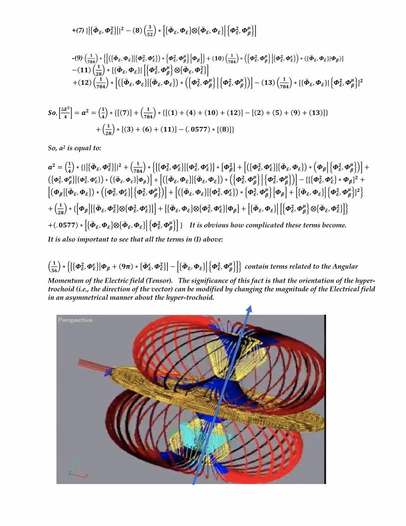
It is also important to see that all the terms in (I) above:
a 𝟏𝟓𝟔b ∗ cde𝜱𝓔
𝟐, 𝜱𝓔𝝐 fg𝜱𝜷 + (𝟗𝝅) ∗ e�̈�𝓔
𝝐 , 𝜱𝓔𝟐fi − je�̈�𝓔, 𝜱𝓔fk c𝜱𝓔
𝟐, 𝜱𝜷𝝁lml contain terms related to the Angular
Momentum of the Electric field (Tensor). The significance of this fact is that the orientation of the hyper-trochoid (i.e., the direction of the vector) can be modified by changing the magnitude of the Electrical field in an asymmetrical manner about the hyper-trochoid.
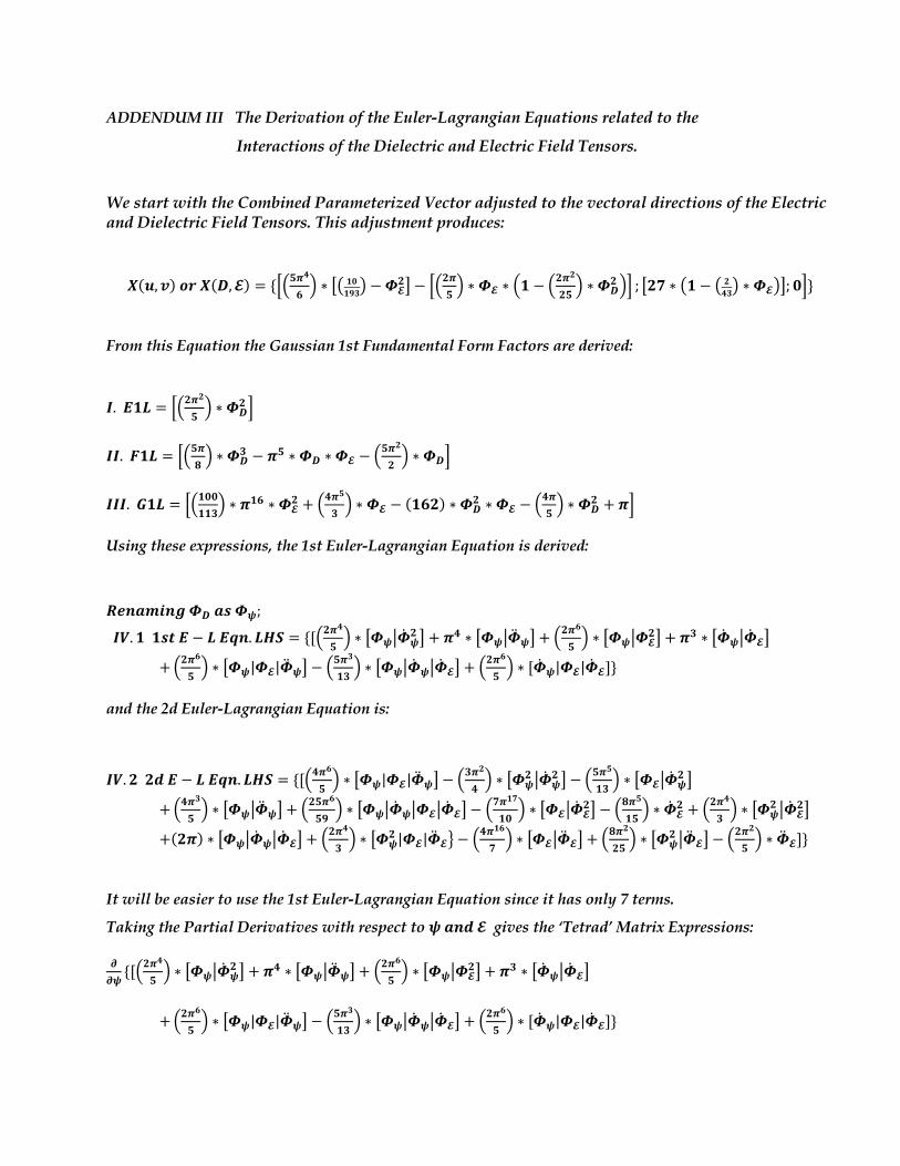
ADDENDUM III The Derivation of the Euler-Lagrangian Equations related to the
Interactions of the Dielectric and Electric Field Tensors.
We start with the Combined Parameterized Vector adjusted to the vectoral directions of the Electric and Dielectric Field Tensors. This adjustment produces:
𝑿(𝒖, 𝒗)𝒐𝒓𝑿(𝑫, 𝓔) = {ja𝟓𝝅𝟒
𝟔b ∗ d� 𝟏𝟎𝟏𝟗𝟑� − 𝜱𝓔
𝟐i − ja𝟐𝝅𝟓b ∗ 𝜱𝓔 ∗ a𝟏 − a
𝟐𝝅𝟐
𝟐𝟓b ∗ 𝜱𝑫
𝟐 bm ; d𝟐𝟕 ∗ �𝟏 − � 𝟐𝟒𝟑� ∗ 𝜱𝓔�i; 𝟎m} From this Equation the Gaussian 1st Fundamental Form Factors are derived:
𝑰.𝑬𝟏𝑳 = ja𝟐𝝅𝟐
𝟓b ∗ 𝜱𝑫
𝟐 m 𝑰𝑰.𝑭𝟏𝑳 = ja𝟓𝝅
𝟖b ∗ 𝜱𝑫
𝟑 − 𝝅𝟓 ∗ 𝜱𝑫 ∗ 𝜱𝓔 − a𝟓𝝅𝟐
𝟐b ∗ 𝜱𝑫m
𝑰𝑰𝑰.𝑮𝟏𝑳 = ja𝟏𝟎𝟎
𝟏𝟏𝟑b ∗ 𝝅𝟏𝟔 ∗ 𝜱𝓔
𝟐 + a𝟒𝝅𝟓
𝟑b ∗ 𝜱𝓔 − (𝟏𝟔𝟐) ∗ 𝜱𝑫
𝟐 ∗ 𝜱𝓔 − a𝟒𝝅𝟓b ∗ 𝜱𝑫
𝟐 + 𝝅m Using these expressions, the 1st Euler-Lagrangian Equation is derived:
𝑹𝒆𝒏𝒂𝒎𝒊𝒏𝒈𝜱𝑫𝒂𝒔𝜱𝝍;
𝑰𝑽. 𝟏𝟏𝒔𝒕𝑬 − 𝑳𝑬𝒒𝒏. 𝑳𝑯𝑺 = {[a𝟐𝝅𝟒
𝟓b ∗ d𝜱𝝍g�̇�𝝍
𝟐 i + 𝝅𝟒 ∗ d𝜱𝝍g�̈�𝝍i + a𝟐𝝅𝟔
𝟓b ∗ d𝜱𝝍g𝜱𝓔
𝟐i + 𝝅𝟑 ∗ d�̇�𝝍g�̇�𝓔i
+a𝟐𝝅𝟔
𝟓b ∗ d𝜱𝝍|𝜱𝓔|�̈�𝝍i − a
𝟓𝝅𝟑
𝟏𝟑b ∗ d𝜱𝝍g�̇�𝝍g�̇�𝓔i + a
𝟐𝝅𝟔
𝟓b ∗ [�̇�𝝍|𝜱𝓔|�̇�𝓔]}
and the 2d Euler-Lagrangian Equation is:
𝑰𝑽. 𝟐𝟐𝒅𝑬 − 𝑳𝑬𝒒𝒏. 𝑳𝑯𝑺 = {[a𝟒𝝅𝟔
𝟓b ∗ d𝜱𝝍|𝜱𝓔|�̈�𝝍i − a
𝟑𝝅𝟐
𝟒b ∗ d𝜱𝝍
𝟐 g�̇�𝝍𝟐 i − a𝟓𝝅
𝟓
𝟏𝟑b ∗ d𝜱𝓔g�̇�𝝍
𝟐 i
+a𝟒𝝅𝟑
𝟓b ∗ d𝜱𝝍g�̈�𝝍i + a
𝟐𝟓𝝅𝟔
𝟓𝟗b ∗ d𝜱𝝍g�̇�𝝍g𝜱𝓔g�̇�𝓔i − a
𝟕𝝅𝟏𝟕
𝟏𝟎b ∗ d𝜱𝓔g�̇�𝓔
𝟐i − a𝟖𝝅𝟓
𝟏𝟓b ∗ �̇�𝓔
𝟐 + a𝟐𝝅𝟒
𝟑b ∗ d𝜱𝝍
𝟐 g�̇�𝓔𝟐i
+(𝟐𝝅) ∗ d𝜱𝝍g�̇�𝝍g�̇�𝓔i + a𝟐𝝅𝟒
𝟑b ∗ d𝜱𝝍
𝟐 |𝜱𝓔|�̈�𝓔f − a𝟒𝝅𝟏𝟔
𝟕b ∗ d𝜱𝓔g�̈�𝓔i + a
𝟖𝝅𝟐
𝟐𝟓b ∗ d𝜱𝝍
𝟐 g�̈�𝓔i − a𝟐𝝅𝟐
𝟓b ∗ �̈�𝓔]}
It will be easier to use the 1st Euler-Lagrangian Equation since it has only 7 terms.
Taking the Partial Derivatives with respect to 𝝍𝒂𝒏𝒅𝓔 gives the ‘Tetrad’ Matrix Expressions: 𝝏𝝏𝝍{[a𝟐𝝅
𝟒
𝟓b ∗ d𝜱𝝍g�̇�𝝍
𝟐 i + 𝝅𝟒 ∗ d𝜱𝝍g�̈�𝝍i + a𝟐𝝅𝟔
𝟓b ∗ d𝜱𝝍g𝜱𝓔
𝟐i + 𝝅𝟑 ∗ d�̇�𝝍g�̇�𝓔i +a𝟐𝝅
𝟔
𝟓b ∗ d𝜱𝝍|𝜱𝓔|�̈�𝝍i − a
𝟓𝝅𝟑
𝟏𝟑b ∗ d𝜱𝝍g�̇�𝝍g�̇�𝓔i + a
𝟐𝝅𝟔
𝟓b ∗ [�̇�𝝍|𝜱𝓔|�̇�𝓔]}
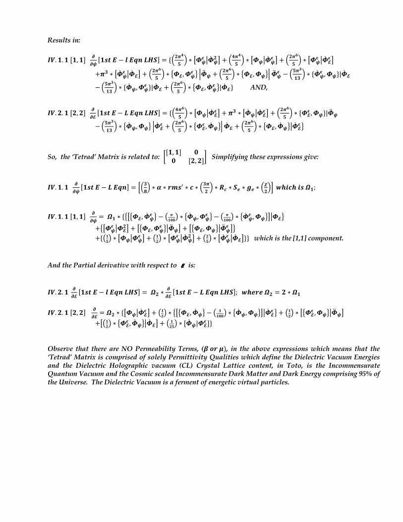
Results in: 𝑰𝑽. 𝟏. 𝟏[𝟏, 𝟏] 𝝏
𝝏𝝍[𝟏𝒔𝒕𝑬 − 𝒍𝑬𝒒𝒏𝑳𝑯𝑺] = {a𝟐𝝅
𝟒
𝟓b ∗ d𝜱𝝍
𝝐 g�̇�𝝍𝟐 i + a𝟒𝝅
𝟒
𝟓b ∗ d𝜱𝝍g�̇�𝝍
𝝐 i + a𝟐𝝅𝟔
𝟓b ∗ d𝜱𝝍
𝝐 g�̇�𝓔𝝐 i
+𝝅𝟑 ∗ d�̇�𝝍𝝐 g�̇�𝓔i + a
𝟐𝝅𝟔
𝟓b ∗ e𝜱𝓔, 𝜱𝝍
𝝐 f k�̈�𝝍 + a𝟐𝝅𝟔
𝟓b ∗ e𝜱𝓔, 𝜱𝝍fk �̈�𝝍
𝝐 − a𝟓𝝅𝟑
𝟏𝟑b ∗ {�̇�𝝍
𝝐 , 𝜱𝝍}|�̇�𝓔
−a𝟓𝝅𝟑
𝟏𝟑b ∗ {�̇�𝝍, 𝜱𝝍
𝝐 }|�̇�𝓔 + a𝟐𝝅𝟔
𝟓b ∗ e𝜱𝓔, �̇�𝝍
𝝐 f|�̇�𝓔} AND,
𝑰𝑽. 𝟐. 𝟏[𝟐, 𝟐] 𝝏𝝏𝓔[𝟏𝒔𝒕𝑬 − 𝑳𝑬𝒒𝒏𝑳𝑯𝑺] = {a𝟒𝝅
𝟔
𝟓b ∗ d𝜱𝝍g�̇�𝓔
𝝐 i + 𝝅𝟑 ∗ d�̇�𝝍g�̇�𝓔𝝐 i + a𝟐𝝅
𝟔
𝟓b ∗ {𝜱𝓔
𝝐 , 𝜱𝝍}|�̈�𝝍
−a𝟓𝝅𝟑
𝟏𝟑b ∗ e�̇�𝝍, 𝜱𝝍f k�̇�𝓔
𝝐 + a𝟐𝝅𝟔
𝟓b ∗ e𝜱𝓔
𝝐 , �̇�𝝍fk �̇�𝓔 + a𝟐𝝅𝟔
𝟓b ∗ e𝜱𝓔, �̇�𝝍fg�̇�𝓔
𝝐f
So, the ‘Tetrad’ Matrix is related to: �[𝟏, 𝟏] 𝟎𝟎 [𝟐, 𝟐]� Simplifying these expressions give:
𝑰𝑽. 𝟏. 𝟏 𝝏𝝏𝝍[𝟏𝒔𝒕𝑬 − 𝑳𝑬𝒒𝒏] = ja𝟑
𝟖b ∗ 𝜶 ∗ 𝒓𝒎𝒔K ∗ 𝒄 ∗ a𝟑𝝅
𝟐b ∗ 𝑹𝒄 ∗ 𝑺𝒆 ∗ 𝒈𝒆 ∗ a
𝝌𝟐bm 𝒘𝒉𝒊𝒄𝒉𝒊𝒔𝜴𝟏;
𝑰𝑽. 𝟏. 𝟏[𝟏, 𝟏] 𝝏𝝏𝝍=𝜴𝟏 ∗ {ede𝜱𝓔, �̇�𝝍
𝝐 f − � 𝝅𝟏𝟎𝟎� ∗ e�̇�𝝍, 𝜱𝝍
𝝐 f − � 𝝅𝟏𝟎𝟎� ∗ e�̇�𝝍
𝝐 , 𝜱𝝍fig𝜱𝓔f +ed𝜱𝝍
𝝐 g𝜱𝓔𝟐i + de𝜱𝓔, 𝜱𝝍
𝝐 fg�̈�𝝍i + de𝜱𝓔, 𝜱𝝍fg�̈�𝝍𝝐 if
+{�𝟏𝟓� ∗ d𝜱𝝍g𝜱𝝍𝝐 i + �𝟏𝟐� ∗ d𝜱𝝍
𝝐 g�̇�𝝍𝟐 i + �𝟐𝟓� ∗ d�̇�𝝍
𝝐 g�̇�𝓔i}} which is the [1,1] component.
And the Partial derivative with respect to ε is:
𝑰𝑽. 𝟐. 𝟏 𝝏𝝏𝓔[𝟏𝒔𝒕𝑬 − 𝒍𝑬𝒒𝒏𝑳𝑯𝑺] = 𝜴𝟐 ∗
𝝏𝝏𝓔[𝟏𝒔𝒕𝑬 − 𝑳𝑬𝒒𝒏𝑳𝑯𝑺]; 𝒘𝒉𝒆𝒓𝒆𝜴𝟐 = 𝟐 ∗ 𝜴𝟏
𝑰𝑽. 𝟐. 𝟏[𝟐, 𝟐] 𝝏
𝝏𝓔= 𝜴𝟐 ∗ {d𝜱𝝍g�̇�𝓔
𝝐 i + �𝟏𝟐� ∗ ede𝜱𝓔, �̇�𝝍f − � 𝟑𝟏𝟎𝟎� ∗ e�̇�𝝍, 𝜱𝝍fig�̇�𝓔
𝝐 f + �𝟏𝟐� ∗ de𝜱𝓔𝝐 , 𝜱𝝍fg�̈�𝝍i
+d�𝟏𝟐� ∗ e𝜱𝓔𝝐 , �̇�𝝍fg�̇�𝓔i + � 𝟏𝟐𝟓� ∗ [�̇�𝝍|𝜱𝓔
𝝐 ]}
Observe that there are NO Permeability Terms, (𝜷𝒐𝒓𝝁), in the above expressions which means that the ‘Tetrad’ Matrix is comprised of solely Permittivity Qualities which define the Dielectric Vacuum Energies and the Dielectric Holographic vacuum (CL) Crystal Lattice content, in Toto, is the Incommensurate Quantum Vacuum and the Cosmic scaled Incommensurate Dark Matter and Dark Energy comprising 95% of the Universe. The Dielectric Vacuum is a ferment of energetic virtual particles.

Taking the cross product of these two expressions produces the Determinant expression:
𝓓U𝓗 = {[𝟎, 𝟎, [j𝜶 ∗ 𝒓𝒎𝒔K ∗ 𝒄 ∗ a𝝅𝟐b ∗ 𝑹𝒄 ∗ 𝑺𝒆 ∗ 𝒈𝒆 ∗ a
𝝌𝒏bm ∗ {(𝟏) cd𝜱𝓔g𝜱𝝍g�̇�𝓔
𝝐 i; e𝜱𝓔, 𝜱𝝍𝝐 fl
(7+13) −a 𝝅
𝟓𝟎b ∗ cd𝜱𝓔g𝜱𝝍g�̇�𝓔
𝜺 i; e�̇�𝝍𝝐 , 𝜱𝝍fl + (𝟏𝟗)ed𝜱𝓔
𝟐g𝜱𝝍g�̇�𝓔𝝐 i;𝜱𝝍
𝝐 f +(𝟐𝟓) cd�̈�𝝍g𝜱𝝍g�̇�𝓔
𝝐 i; e𝜱𝓔, 𝜱𝝍𝝐 fl + (𝟑𝟏) cd�̈�𝝍
𝝐 g𝜱𝝍g�̇�𝓔𝝐 i; e𝜱𝓔, 𝜱𝝍fl
+(𝟑𝟕) a𝟏
𝟓b ∗ ed𝜱𝝍
𝝐 g𝜱𝝍g𝜱𝓔𝝐 i;𝜱𝝍f + (𝟒𝟑) a
𝟏𝟐b ∗ ed�̇�𝝍
𝟐 g𝜱𝝍g�̇�𝓔𝝐 i;𝜱𝝍
𝝐 f +(𝟒𝟗) a𝟐
𝟓b ∗ ed�̇�𝓔g𝜱𝝍g�̇�𝓔
𝝐 i; �̇�𝝍𝝐 f + (𝟐) a𝟏
𝟒b ∗ cd𝜱𝓔ge𝜱𝓔, �̇�𝝍fg�̇�𝓔
𝝐 i; e𝜱𝓔, �̇�𝝍𝝐 fl
−(𝟖) J 𝝅
𝟐𝟎𝟎K ∗ LM𝜱𝓔NO𝜱𝓔, �̇�𝝍PN�̇�𝓔
𝝐 Q; O�̇�𝝍, 𝜱𝝍𝝐 PS − (𝟏𝟒) J 𝝅
𝟐𝟎𝟎K ∗ LM𝜱𝓔NO𝜱𝓔, �̇�𝝍PN�̇�𝓔
𝝐 Q; O𝜱𝓔, �̇�𝝍PS +(𝟐𝟎) a𝟏
𝟐b ∗ {d𝜱𝓔
𝟐ge𝜱𝓔, �̇�𝝍fg𝜱𝓔𝝐 i;𝜱𝝍
𝝐 }} + (𝟐𝟔)(𝟏𝟐) ∗ {d�̈�𝝍ge𝜱𝓔, �̇�𝝍fg𝜱𝓔
𝝐 i; {𝜱𝓔, 𝜱𝝍𝝐 }}
+(𝟑𝟐) a𝟏
𝟐b ∗ cd�̈�𝝍
𝝐 ge𝜱𝓔, �̇�𝝍fg�̇�𝓔𝝐 i; e𝜱𝓔, 𝜱𝝍fl + (𝟑𝟖) a
𝟏𝟏𝟎b ∗ ed𝜱𝝍
𝝐 ge𝜱𝓔, �̇�𝝍fg�̇�𝓔𝝐 i;𝜱𝝍f
+(𝟒𝟒) a𝟏
𝟒b ∗ ed�̇�𝝍
𝟐 ge𝜱𝓔, �̇�𝝍fg�̇�𝓔𝝐 i;𝜱𝝍
𝝐 f + (𝟓𝟎) a𝟏𝟓b ∗ ed�̇�𝓔ge𝜱𝓔, �̇�𝝍fg�̇�𝓔
𝝐 i;𝜱𝝍𝝐 f
+(𝟑)cd𝜱𝓔ge𝜱𝝍, 𝜱𝝍fg𝜱𝓔𝝐 i; e𝜱𝓔, 𝜱𝝍
𝝐 fl + (𝟐𝟏) a 𝟑𝟏𝟎𝟎b ∗ ed𝜱𝓔
𝟐ge�̇�𝝍, 𝜱𝝍fg�̇�𝓔𝜺 i;𝜱𝝍
𝝐 f +(𝟐𝟕) J 𝟑
𝟏𝟎𝟎K ∗ LM�̈�𝝍NO�̇�𝝍, 𝜱𝝍PN�̇�𝓔
𝝐 Q; {𝜱𝓔, 𝜱𝓔𝝐 }S + (𝟑𝟑)J 𝟑
𝟏𝟎𝟎K ∗ LM�̈�𝝍
𝝐 NO�̇�𝝍, 𝜱𝝍PN�̇�𝓔𝝐 Q; O𝜱𝓔, 𝜱𝝍PS
+(𝟒𝟓)a 𝟑
𝟒𝟎𝟎b ∗ ed�̇�𝝍
𝟐 ge�̇�𝝍, 𝜱𝝍fg�̇�𝓔𝝐 i;𝜱𝝍
𝝐 f + (𝟓𝟏) a 𝟑𝟏𝟎𝟎b ∗ ed�̇�𝓔ge�̇�𝝍, 𝜱𝝍fg�̇�𝓔
𝝐 i; �̇�𝝍𝝐 f
Note: Terms (9), (15) and (39) are deleted due to their contribution being insignificant. +(𝟒)J𝟏
𝟐K ∗ LM𝜱𝓔NO𝜱𝓔
𝝐 , 𝜱𝝍PN�̈�𝝍Q; O𝜱𝓔, �̇�𝝍PS − (𝟏𝟎) J𝝅𝟏𝟎𝟎K ∗ LM𝜱𝓔NO𝜱𝓔
𝝐 , 𝜱𝝍PN�̈�𝝍Q; O�̇�𝝍, 𝜱𝝍𝝐 PS
−(𝟏𝟔) a 𝝅
𝟐𝟎𝟎b ∗ cd𝜱𝓔ge𝜱𝓔
𝝐 , 𝜱𝝍fg�̈�𝝍i; e�̇�𝝍𝝐 , 𝜱𝝍fl + (𝟐𝟐) a
𝟏𝟐b ∗ ed𝜱𝓔
𝟐ge𝜱𝓔𝝐 , 𝜱𝝍fg�̈�𝝍i;𝜱𝝍
𝝐 f +(𝟐𝟖) J𝟏
𝟐K ∗ LM�̈�𝝍NO𝜱𝓔
𝝐 , 𝜱𝝍PN�̈�𝝍Q; O𝜱𝓔, 𝜱𝝍𝝐 PS + (𝟑𝟒) J𝟏
𝟐K ∗ LM�̈�𝝍
𝝐 NO𝜱𝓔𝝐 , 𝜱𝝍PN�̈�𝝍QO𝜱𝓔, 𝜱𝝍PS
+(𝟒𝟎)a 𝟏
𝟏𝟎b ∗ ed𝜱𝝍
𝝐 ge𝜱𝓔𝝐 , 𝜱𝝍fg�̈�𝝍i;𝜱𝝍f + (𝟒𝟔) a
𝟏𝟒b ∗ ed�̇�𝝍
𝟐 ge𝜱𝓔𝝐 , 𝜱𝝍f|�̈�𝝍i;𝜱𝝍
𝝐 f +(𝟓𝟐)a𝟏
𝟓b ∗ ed�̇�𝓔ge𝜱𝓔
𝝐 , 𝜱𝝍fg�̈�𝝍i; �̇�𝝍𝝐 f − (𝟓, 𝟒𝟕)a 𝟓
𝟏𝟑b ∗ ed𝜱𝓔
𝝐 ge𝜱𝓔𝝐 , �̇�𝝍fg�̇�𝓔i; �̇�𝝍f
−(𝟏𝟏)J 𝝅
𝟐𝟎𝟎K ∗ LM𝜱𝓔NO𝜱𝓔
𝝐 , �̇�𝝍PN�̇�𝓔Q; O�̇�𝝍, 𝜱𝝍𝝐 PS − (𝟏𝟕) J 𝝅
𝟐𝟎𝟎K ∗ LM𝜱𝓔NO𝜱𝓔
𝝐 , �̇�𝝍PN𝜱𝓔Q; O�̇�𝝍𝝐 , 𝜱𝝍PS
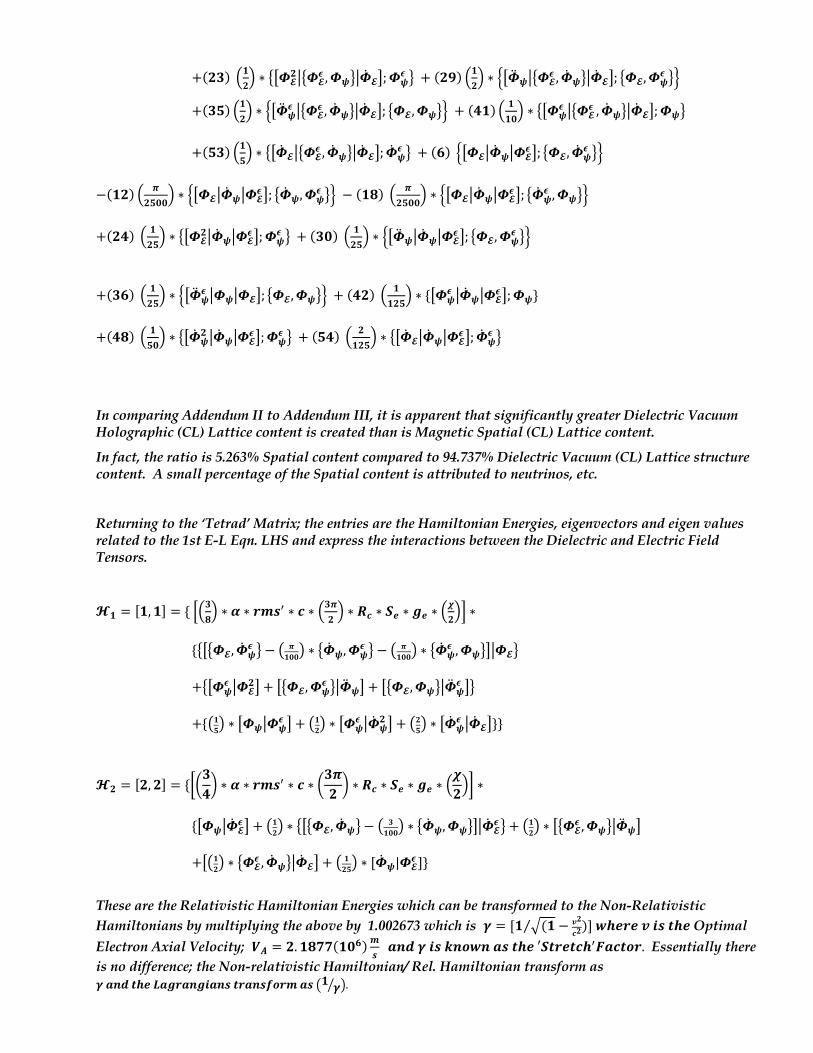
+(𝟐𝟑)a𝟏
𝟐b ∗ ed𝜱𝓔
𝟐ge𝜱𝓔𝝐 , 𝜱𝝍fg�̇�𝓔i;𝜱𝝍
𝝐 f + (𝟐𝟗) a𝟏𝟐b ∗ cd�̈�𝝍ge𝜱𝓔
𝝐 , �̇�𝝍fg�̇�𝓔i; e𝜱𝓔, 𝜱𝝍𝝐 fl
+(𝟑𝟓) a𝟏𝟐b ∗ cd�̈�𝝍
𝝐 ge𝜱𝓔𝝐 , �̇�𝝍fg�̇�𝓔i; e𝜱𝓔, 𝜱𝝍fl + (𝟒𝟏) a
𝟏𝟏𝟎b ∗ ed𝜱𝝍
𝝐 ge𝜱𝓔𝝐, �̇�𝝍fg�̇�𝓔i;𝜱𝝍f
+(𝟓𝟑) a𝟏
𝟓b ∗ ed�̇�𝓔ge𝜱𝓔
𝝐 , �̇�𝝍fg�̇�𝓔i; �̇�𝝍𝝐 f + (𝟔)cd𝜱𝓔g�̇�𝝍g𝜱𝓔
𝝐 i; e𝜱𝓔, �̇�𝝍𝝐 fl
−(𝟏𝟐) a 𝝅
𝟐𝟓𝟎𝟎b ∗ cd𝜱𝓔g�̇�𝝍g𝜱𝓔
𝝐 i; e�̇�𝝍, 𝜱𝝍𝝐 fl − (𝟏𝟖)a 𝝅
𝟐𝟓𝟎𝟎b ∗ cd𝜱𝓔g�̇�𝝍g𝜱𝓔
𝝐 i; e�̇�𝝍𝝐 , 𝜱𝝍fl
+(𝟐𝟒)a 𝟏
𝟐𝟓b ∗ ed𝜱𝓔
𝟐g�̇�𝝍g𝜱𝓔𝝐 i;𝜱𝝍
𝝐 f + (𝟑𝟎)a 𝟏𝟐𝟓b ∗ cd�̈�𝝍g�̇�𝝍g𝜱𝓔
𝝐 i; e𝜱𝓔, 𝜱𝝍𝝐 fl
+(𝟑𝟔)a 𝟏
𝟐𝟓b ∗ cd�̈�𝝍
𝝐 g𝜱𝝍g𝜱𝓔i; e𝜱𝓔, 𝜱𝝍fl + (𝟒𝟐)a𝟏𝟏𝟐𝟓b ∗ {d𝜱𝝍
𝝐 g�̇�𝝍g𝜱𝓔𝝐 i;𝜱𝝍}
+(𝟒𝟖)a 𝟏
𝟓𝟎b ∗ ed�̇�𝝍
𝟐 g�̇�𝝍g𝜱𝓔𝝐 i;𝜱𝝍
𝝐 f + (𝟓𝟒)a 𝟐𝟏𝟐𝟓b ∗ ed�̇�𝓔g�̇�𝝍g𝜱𝓔
𝝐 i; �̇�𝝍𝝐 f
In comparing Addendum II to Addendum III, it is apparent that significantly greater Dielectric Vacuum Holographic (CL) Lattice content is created than is Magnetic Spatial (CL) Lattice content.
In fact, the ratio is 5.263% Spatial content compared to 94.737% Dielectric Vacuum (CL) Lattice structure content. A small percentage of the Spatial content is attributed to neutrinos, etc.
Returning to the ‘Tetrad’ Matrix; the entries are the Hamiltonian Energies, eigenvectors and eigen values related to the 1st E-L Eqn. LHS and express the interactions between the Dielectric and Electric Field Tensors.
𝓗𝟏 = [𝟏, 𝟏] = {ja𝟑𝟖b ∗ 𝜶 ∗ 𝒓𝒎𝒔K ∗ 𝒄 ∗ a𝟑𝝅
𝟐b ∗ 𝑹𝒄 ∗ 𝑺𝒆 ∗ 𝒈𝒆 ∗ a
𝝌𝟐bm ∗
{ede𝜱𝓔, �̇�𝝍
𝝐 f − � 𝝅𝟏𝟎𝟎� ∗ e�̇�𝝍, 𝜱𝝍
𝝐 f − � 𝝅𝟏𝟎𝟎� ∗ e�̇�𝝍
𝝐 , 𝜱𝝍fig𝜱𝓔f +ed𝜱𝝍
𝝐 g𝜱𝓔𝟐i + de𝜱𝓔, 𝜱𝝍
𝝐 fg�̈�𝝍i + de𝜱𝓔, 𝜱𝝍fg�̈�𝝍𝝐 if
+{�𝟏𝟓� ∗ d𝜱𝝍g𝜱𝝍
𝝐 i + �𝟏𝟐� ∗ d𝜱𝝍𝝐 g�̇�𝝍
𝟐 i + �𝟐𝟓� ∗ d�̇�𝝍𝝐 g�̇�𝓔i}}
𝓗𝟐 = [𝟐, 𝟐] = {��𝟑𝟒� ∗ 𝜶 ∗ 𝒓𝒎𝒔
K ∗ 𝒄 ∗ �𝟑𝝅𝟐 � ∗ 𝑹𝒄 ∗ 𝑺𝒆 ∗ 𝒈𝒆 ∗ a
𝝌𝟐b� ∗
{d𝜱𝝍g�̇�𝓔
𝝐 i + �𝟏𝟐� ∗ ede𝜱𝓔, �̇�𝝍f − � 𝟑𝟏𝟎𝟎� ∗ e�̇�𝝍, 𝜱𝝍fig�̇�𝓔
𝝐 f + �𝟏𝟐� ∗ de𝜱𝓔𝝐 , 𝜱𝝍fg�̈�𝝍i
+d�𝟏𝟐� ∗ e𝜱𝓔
𝝐 , �̇�𝝍fg�̇�𝓔i + � 𝟏𝟐𝟓� ∗ [�̇�𝝍|𝜱𝓔𝝐 ]}
These are the Relativistic Hamiltonian Energies which can be transformed to the Non-Relativistic Hamiltonians by multiplying the above by 1.002673 which is 𝜸 = [𝟏 �(𝟏 − 𝒗𝟐
𝒄𝟐)]𝒘𝒉𝒆𝒓𝒆𝒗𝒊𝒔𝒕𝒉𝒆⁄ Optimal
Electron Axial Velocity; 𝑽𝑨 = 𝟐. 𝟏𝟖𝟕𝟕(𝟏𝟎𝟔)𝒎𝒔𝒂𝒏𝒅𝜸𝒊𝒔𝒌𝒏𝒐𝒘𝒏𝒂𝒔𝒕𝒉𝒆′𝑺𝒕𝒓𝒆𝒕𝒄𝒉K𝑭𝒂𝒄𝒕𝒐𝒓. Essentially there
is no difference; the Non-relativistic Hamiltonian/ Rel. Hamiltonian transform as 𝜸𝒂𝒏𝒅𝒕𝒉𝒆𝑳𝒂𝒈𝒓𝒂𝒏𝒈𝒊𝒂𝒏𝒔𝒕𝒓𝒂𝒏𝒔𝒇𝒐𝒓𝒎𝒂𝒔S𝟏 𝜸` X.
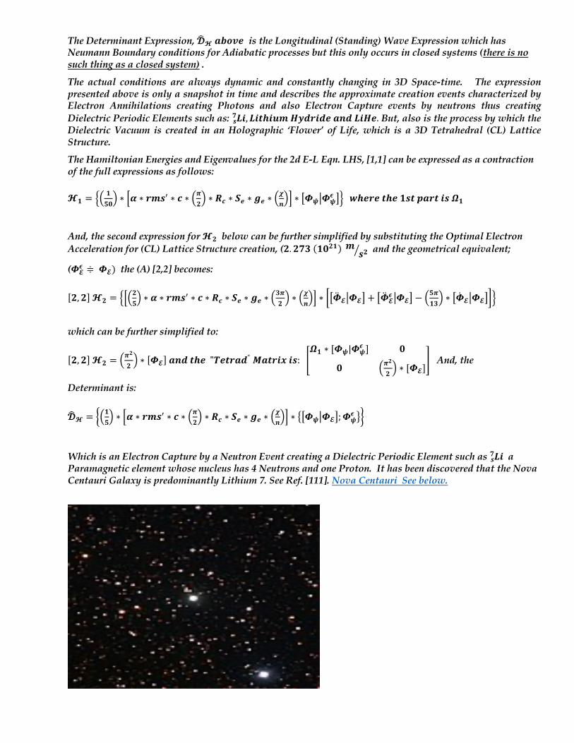
The Determinant Expression, 𝓓U𝓗𝒂𝒃𝒐𝒗𝒆 is the Longitudinal (Standing) Wave Expression which has Neumann Boundary conditions for Adiabatic processes but this only occurs in closed systems (there is no such thing as a closed system) .
The actual conditions are always dynamic and constantly changing in 3D Space-time. The expression presented above is only a snapshot in time and describes the approximate creation events characterized by Electron Annihilations creating Photons and also Electron Capture events by neutrons thus creating Dielectric Periodic Elements such as: 𝑳𝒊𝒔
𝟕 , 𝑳𝒊𝒕𝒉𝒊𝒖𝒎𝑯𝒚𝒅𝒓𝒊𝒅𝒆𝒂𝒏𝒅𝑳𝒊𝑯𝒆. But, also is the process by which the Dielectric Vacuum is created in an Holographic ‘Flower’ of Life, which is a 3D Tetrahedral (CL) Lattice Structure.
The Hamiltonian Energies and Eigenvalues for the 2d E-L Eqn. LHS, [1,1] can be expressed as a contraction of the full expressions as follows: 𝓗𝟏 = ca 𝟏
𝟓𝟎b ∗ j𝜶 ∗ 𝒓𝒎𝒔K ∗ 𝒄 ∗ a𝝅
𝟐b ∗ 𝑹𝒄 ∗ 𝑺𝒆 ∗ 𝒈𝒆 ∗ a
𝝌𝒏bm ∗ d𝜱𝝍g𝜱𝝍
𝝐 il 𝒘𝒉𝒆𝒓𝒆𝒕𝒉𝒆𝟏𝒔𝒕𝒑𝒂𝒓𝒕𝒊𝒔𝜴𝟏
And, the second expression for 𝓗𝟐 below can be further simplified by substituting the Optimal Electron Acceleration for (CL) Lattice Structure creation, (𝟐. 𝟐𝟕𝟑(𝟏𝟎𝟐𝟏)𝒎 𝒔𝟐� and the geometrical equivalent;
(𝜱𝓔𝝐 ≑𝜱𝓔) the (A) [2,2] becomes:
[𝟐, 𝟐]𝓗𝟐 = cja𝟐
𝟓b ∗ 𝜶 ∗ 𝒓𝒎𝒔K ∗ 𝒄 ∗ 𝑹𝒄 ∗ 𝑺𝒆 ∗ 𝒈𝒆 ∗ a
𝟑𝝅𝟐b ∗ a𝝌
𝒏bm ∗ �d�̈�𝓔g𝜱𝓔i + d�̈�𝓔
𝝐 g𝜱𝓔i − a𝟓𝝅𝟏𝟑b ∗ d�̇�𝓔g𝜱𝓔i�l
which can be further simplified to:
[𝟐, 𝟐]𝓗𝟐 = a𝝅𝟐
𝟐b ∗ [𝜱𝓔]𝒂𝒏𝒅𝒕𝒉𝒆"𝑻𝒆𝒕𝒓𝒂𝒅"𝑴𝒂𝒕𝒓𝒊𝒙𝒊𝒔: �
𝜴𝟏 ∗ [𝜱𝝍|𝜱𝝍𝝐 ] 𝟎
𝟎 a𝝅𝟐
𝟐b ∗ [𝜱𝓔]
� And, the
Determinant is: 𝓓U𝓗 = �a𝟏
𝟓b ∗ j𝜶 ∗ 𝒓𝒎𝒔K ∗ 𝒄 ∗ a𝝅
𝟐b ∗ 𝑹𝒄 ∗ 𝑺𝒆 ∗ 𝒈𝒆 ∗ a
𝝌𝒏bm ∗ ed𝜱𝝍g𝜱𝓔i;𝜱𝝍
𝝐 f�
Which is an Electron Capture by a Neutron Event creating a Dielectric Periodic Element such as 𝑳𝒊𝒔𝟕 a
Paramagnetic element whose nucleus has 4 Neutrons and one Proton. It has been discovered that the Nova Centauri Galaxy is predominantly Lithium 7. See Ref. [111]. Nova Centauri See below.
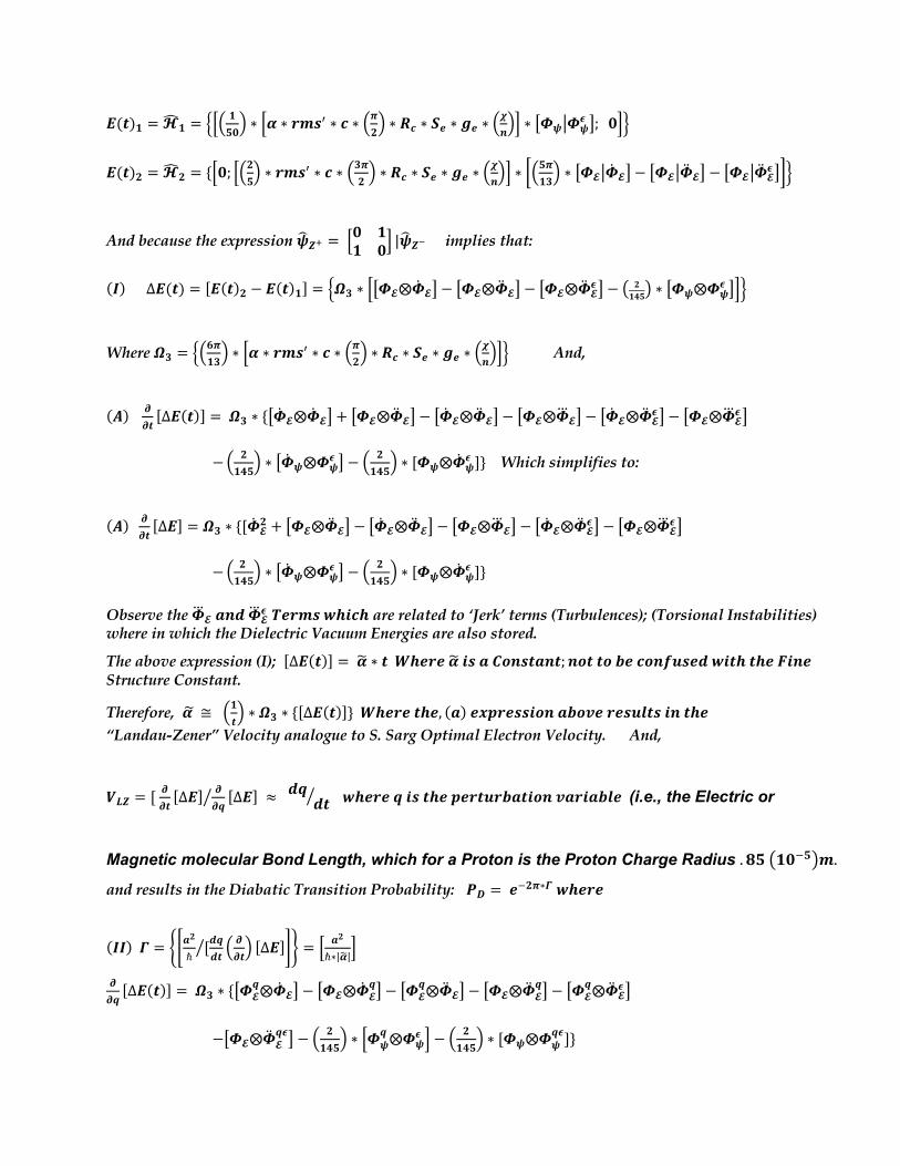
𝑬(𝒕)𝟏 = 𝓗Q𝟏 = cja 𝟏
𝟓𝟎b ∗ j𝜶 ∗ 𝒓𝒎𝒔K ∗ 𝒄 ∗ a𝝅
𝟐b ∗ 𝑹𝒄 ∗ 𝑺𝒆 ∗ 𝒈𝒆 ∗ a
𝝌𝒏bm ∗ d𝜱𝝍g𝜱𝝍
𝝐 i; 𝟎ml 𝑬(𝒕)𝟐 = 𝓗Q𝟐 = {j𝟎; ja𝟐
𝟓b ∗ 𝒓𝒎𝒔K ∗ 𝒄 ∗ a𝟑𝝅
𝟐b ∗ 𝑹𝒄 ∗ 𝑺𝒆 ∗ 𝒈𝒆 ∗ a
𝝌𝒏bm ∗ �a𝟓𝝅
𝟏𝟑b ∗ d𝜱𝓔g�̇�𝓔i − d𝜱𝓔g�̈�𝓔i − d𝜱𝓔g�̈�𝓔
𝝐 i�l
And because the expression 𝝍U𝒁2 = j𝟎 𝟏𝟏 𝟎m |𝝍
U𝒁3 implies that: (𝑰)∆𝑬(𝒕) = [𝑬(𝒕)𝟐 − 𝑬(𝒕)𝟏] = c𝜴𝟑 ∗ jd𝜱𝓔⨂�̇�𝓔i − d𝜱𝓔⨂�̈�𝓔i − d𝜱𝓔⨂�̈�𝓔
𝝐 i − � 𝟐𝟏𝟒𝟓� ∗ d𝜱𝝍⨂𝜱𝝍
𝝐 iml
Where 𝜴𝟑 = ca𝟔𝝅𝟏𝟑b ∗ j𝜶 ∗ 𝒓𝒎𝒔K ∗ 𝒄 ∗ a𝝅
𝟐b ∗ 𝑹𝒄 ∗ 𝑺𝒆 ∗ 𝒈𝒆 ∗ a
𝝌𝒏bml And,
(𝑨) 𝝏𝝏𝒕[∆𝑬(𝒕)] = 𝜴𝟑 ∗ {d�̇�𝓔⨂�̇�𝓔i + d𝜱𝓔⨂�̈�𝓔i − d�̇�𝓔⨂�̈�𝓔i − d𝜱𝓔⨂𝜱�𝓔i − d�̇�𝓔⨂�̈�𝓔
𝝐 i − d𝜱𝓔⨂𝜱�𝓔𝝐 i −a 𝟐
𝟏𝟒𝟓b ∗ d�̇�𝝍⨂𝜱𝝍
𝝐 i − a 𝟐𝟏𝟒𝟓b ∗ [𝜱𝝍⨂�̇�𝝍
𝝐 ]} Which simplifies to:
(𝑨) 𝝏𝝏𝒕[∆𝑬] = 𝜴𝟑 ∗ {[�̇�𝓔
𝟐 + d𝜱𝓔⨂�̈�𝓔i − d�̇�𝓔⨂�̈�𝓔i − d𝜱𝓔⨂𝜱�𝓔i − d�̇�𝓔⨂�̈�𝓔𝝐 i − d𝜱𝓔⨂𝜱�𝓔𝝐 i
−a 𝟐
𝟏𝟒𝟓b ∗ d�̇�𝝍⨂𝜱𝝍
𝝐 i − a 𝟐𝟏𝟒𝟓b ∗ [𝜱𝝍⨂�̇�𝝍
𝝐 ]} Observe the 𝜱�𝓔𝒂𝒏𝒅𝜱� 𝓔𝝐 𝑻𝒆𝒓𝒎𝒔𝒘𝒉𝒊𝒄𝒉 are related to ‘Jerk’ terms (Turbulences); (Torsional Instabilities) where in which the Dielectric Vacuum Energies are also stored.
The above expression (I); [∆𝑬(𝒕)] = 𝜶� ∗ 𝒕𝑾𝒉𝒆𝒓𝒆𝜶�𝒊𝒔𝒂𝑪𝒐𝒏𝒔𝒕𝒂𝒏𝒕; 𝒏𝒐𝒕𝒕𝒐𝒃𝒆𝒄𝒐𝒏𝒇𝒖𝒔𝒆𝒅𝒘𝒊𝒕𝒉𝒕𝒉𝒆𝑭𝒊𝒏𝒆 Structure Constant.
Therefore, 𝜶� ≅ a𝟏𝒕b ∗ 𝜴𝟑 ∗ {[∆𝑬(𝒕)]}𝑾𝒉𝒆𝒓𝒆𝒕𝒉𝒆, (𝒂)𝒆𝒙𝒑𝒓𝒆𝒔𝒔𝒊𝒐𝒏𝒂𝒃𝒐𝒗𝒆𝒓𝒆𝒔𝒖𝒍𝒕𝒔𝒊𝒏𝒕𝒉𝒆
“Landau-Zener” Velocity analogue to S. Sarg Optimal Electron Velocity. And,
𝑽𝑳𝒁 = [ 𝝏𝝏𝒕[∆𝑬] 𝝏
𝝏𝒒[∆𝑬]� ≈ 𝒅𝒒 𝒅𝒕� 𝒘𝒉𝒆𝒓𝒆𝒒𝒊𝒔𝒕𝒉𝒆𝒑𝒆𝒓𝒕𝒖𝒓𝒃𝒂𝒕𝒊𝒐𝒏𝒗𝒂𝒓𝒊𝒂𝒃𝒍𝒆 (i.e., the Electric or
Magnetic molecular Bond Length, which for a Proton is the Proton Charge Radius . 𝟖𝟓L𝟏𝟎0𝟓P𝒎.
and results in the Diabatic Transition Probability: 𝑷𝑫 =𝒆:𝟐𝝅∗𝜞𝒘𝒉𝒆𝒓𝒆
(𝑰𝑰)𝜞 = �^𝒂𝟐
ℏ[𝒅𝒒𝒅𝒕
� a 𝝏𝝏𝒕b [∆𝑬]_� = j 𝒂𝟐
ℏ∗|𝜶G|m
𝝏𝝏𝒒[∆𝑬(𝒕)] = 𝜴𝟑 ∗ {d𝜱𝓔
𝒒⨂�̇�𝓔i − d𝜱𝓔⨂�̇�𝓔𝒒i − d𝜱𝓔
𝒒⨂�̈�𝓔i − d𝜱𝓔⨂�̈�𝓔𝒒i − d𝜱𝓔
𝒒⨂�̈�𝓔𝝐 i
−d𝜱𝓔⨂�̈�𝓔
𝒒𝝐i − a 𝟐𝟏𝟒𝟓b ∗ j𝜱𝝍
𝒒⨂𝜱𝝍𝝐 m − a 𝟐
𝟏𝟒𝟓b ∗ [𝜱𝝍⨂𝜱𝝍
𝒒𝝐]}
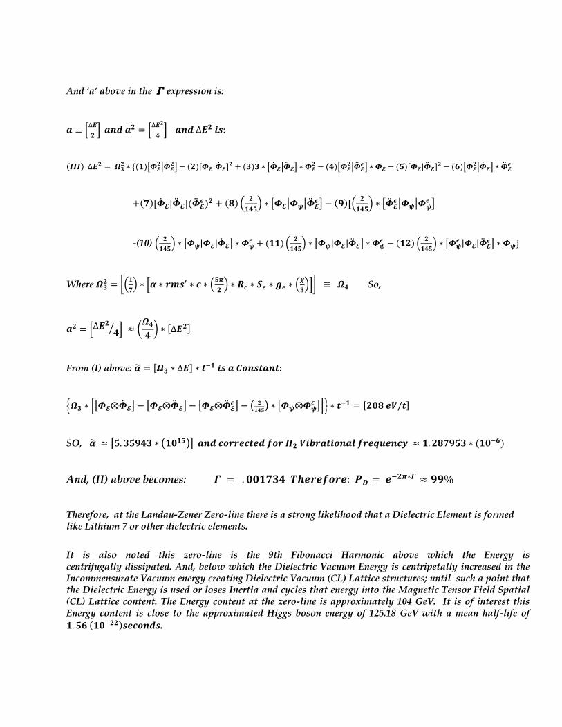
And ‘a’ above in the Г expression is:
𝒂 ≡ j∆𝑬𝟐m 𝒂𝒏𝒅𝒂𝟐 = j∆𝑬
𝟐
𝟒m 𝒂𝒏𝒅∆𝑬𝟐𝒊𝒔:
(𝑰𝑰𝑰)∆𝑬𝟐 =𝜴𝟑𝟐 ∗ {(𝟏)e𝜱𝓔𝟐W�̇�𝓔
𝟐f − (𝟐)[𝜱𝓔|�̇�𝓔]𝟐 + (𝟑)𝟑 ∗ e�̇�𝓔W�̈�𝓔f ∗ 𝜱𝓔𝟐 − (𝟒)e𝜱𝓔
𝟐W�̈�𝓔𝝐 f ∗ 𝜱𝓔 − (𝟓)[𝜱𝓔|�̈�𝓔]𝟐 − (𝟔)e𝜱𝓔
𝟐W�̇�𝓔f ∗ �̈�𝓔𝝐
+(𝟕)[�̇�𝓔|�̈�𝓔|(�̈�𝓔𝝐)𝟐 + (𝟖) a 𝟐
𝟏𝟒𝟓b ∗ d𝜱𝓔g𝜱𝝍g�̈�𝓔
𝝐 i − (𝟗)[a 𝟐𝟏𝟒𝟓b ∗ d�̈�𝓔
𝝐 g𝜱𝝍g𝜱𝝍𝝐 i
-(10) J 𝟐𝟏𝟒𝟓K ∗ M𝜱𝝍|𝜱𝓔|�̇�𝓔Q ∗ 𝜱𝝍
𝝐 + (𝟏𝟏) J 𝟐𝟏𝟒𝟓K ∗ M𝜱𝝍|𝜱𝓔|�̈�𝓔Q ∗ 𝜱𝝍
𝝐 − (𝟏𝟐) J 𝟐𝟏𝟒𝟓K ∗ M𝜱𝝍
𝝐 |𝜱𝓔|�̈�𝓔𝝐 Q ∗ 𝜱𝝍}
Where 𝜴𝟑𝟐 = �a𝟏𝟕b ∗ j𝜶 ∗ 𝒓𝒎𝒔K ∗ 𝒄 ∗ a𝟓𝝅
𝟐b ∗ 𝑹𝒄 ∗ 𝑺𝒆 ∗ 𝒈𝒆 ∗ a
𝝌𝟑bm� ≡ 𝜴𝟒 So,
𝒂𝟐 = j∆𝑬𝟐𝟒� m ≈ �
𝜴𝟒𝟒 � ∗
[∆𝑬𝟐]
From (I) above: 𝜶� = [𝜴𝟑 ∗ ∆𝑬] ∗ 𝒕:𝟏𝒊𝒔𝒂𝑪𝒐𝒏𝒔𝒕𝒂𝒏𝒕:
c𝜴𝟑 ∗ jd𝜱𝓔⨂�̇�𝓔i − d𝜱𝓔⨂�̈�𝓔i − d𝜱𝓔⨂�̈�𝓔𝝐 i − � 𝟐
𝟏𝟒𝟓� ∗ d𝜱𝝍⨂𝜱𝝍𝝐 iml ∗ 𝒕:𝟏 = [𝟐𝟎𝟖𝒆𝑽/𝒕]
SO, 𝜶� ≃ d𝟓. 𝟑𝟓𝟗𝟒𝟑 ∗ �𝟏𝟎𝟏𝟓�i𝒂𝒏𝒅𝒄𝒐𝒓𝒓𝒆𝒄𝒕𝒆𝒅𝒇𝒐𝒓𝑯𝟐𝑽𝒊𝒃𝒓𝒂𝒕𝒊𝒐𝒏𝒂𝒍𝒇𝒓𝒆𝒒𝒖𝒆𝒏𝒄𝒚 ≈ 𝟏. 𝟐𝟖𝟕𝟗𝟓𝟑 ∗ (𝟏𝟎:𝟔)
And, (II) above becomes: 𝜞 =. 𝟎𝟎𝟏𝟕𝟑𝟒𝑻𝒉𝒆𝒓𝒆𝒇𝒐𝒓𝒆:𝑷𝑫 =𝒆1𝟐𝝅∗𝜞 ≈ 𝟗𝟗%
Therefore, at the Landau-Zener Zero-line there is a strong likelihood that a Dielectric Element is formed like Lithium 7 or other dielectric elements.
It is also noted this zero-line is the 9th Fibonacci Harmonic above which the Energy is centrifugally dissipated. And, below which the Dielectric Vacuum Energy is centripetally increased in the Incommensurate Vacuum energy creating Dielectric Vacuum (CL) Lattice structures; until such a point that the Dielectric Energy is used or loses Inertia and cycles that energy into the Magnetic Tensor Field Spatial (CL) Lattice content. The Energy content at the zero-line is approximately 104 GeV. It is of interest this Energy content is close to the approximated Higgs boson energy of 125.18 GeV with a mean half-life of 𝟏. 𝟓𝟔(𝟏𝟎:𝟐𝟐)𝒔𝒆𝒄𝒐𝒏𝒅𝒔.
As an example, in the above case of Lithium 7 formation, the formation time is approximately 1.7645 (𝟏𝟎:𝟐𝟐)𝒔𝒆𝒄𝒐𝒏𝒅𝒔. This information corresponds closely to the above. Once again, this is a dynamic creation event process; above the zero-line the probability drops off quickly at a𝝌
𝒏b , 𝒐𝒓𝟗𝟗%; 𝟓𝟎%;𝟑𝟑%; etc. at
multiples of the Fibonacci Harmonics/ sub-Harmonics. [𝟒𝟔] − [𝟒𝟗]; [72]
Below the zero-line the energy concentration increases for each of the 9th sub-Harmonics until convergence into the Incommensurable Dielectric Vacuum (CL) Lattice Content structures. It is also noted the open system of the Dielectric Vacuum has a maximum of stored energy. This stored Quantum Vacuum Energy is estimated at 𝝆𝒗 = 𝟓. 𝟏𝟓𝟕(𝟏𝟎𝟏𝟎𝟐)𝒌𝒈/𝒎𝟑 As long as this energy is stored it can be used for work. It is what Schrödinger referred to as negative entropy (negentropy) and later corrected the phrase to ‘stored energy’. “The Vacuum is an energetic and dynamic medium …which contains causative dynamics which when interacted with mass will and do generate all observed forces and changes in the physical ‘Spatial’ system. As an electron moves through space it is actually swimming through a sea of ‘ghost’ particles of all varieties, leptons, quarks, and ‘messengers’, entangled in a complex 𝒎𝒆§𝒍�́�𝒆. An Electron will distort this irreducible vacuum activity, and the distortion reacts back on the Electron. Even at rest, an Electron is not at ‘rest’; it is being assaulted by all manner of other particles from the Vacuum.” [129]
Furthermore, …” In General Relativity (GR), if there is a mass or charge anywhere in the Universe, then the whole of Spacetime is curved, and all the laws of physics must be written in curved spacetime, including, of course, the laws of Electrodynamics.” [130] This energy is stored in both information and Negentropy characterized by the entropy production expression in which 𝑰𝑺𝑬 is the Information between the system and the environment where: (𝑨)𝝈 = 𝑰𝑺𝑬 +𝑫d𝝆𝑬(𝒕)g𝝆𝓔
𝒆𝒒i𝒘𝒉𝒆𝒓𝒆𝝆𝓔𝒆𝒒𝒊𝒔𝒕𝒉𝒆𝑮𝒊𝒃𝒃𝒔𝒔𝒕𝒂𝒕𝒆𝒐𝒇𝒕𝒉𝒆𝒆𝒏𝒗𝒊𝒓𝒐𝒏𝒎𝒆𝒏𝒕.
𝑫d𝝆𝑬(𝒕)g𝝆𝓔𝒆𝒒iis the relative entropy the original and final state of the environment. The 𝑰𝑺𝑬𝒊𝒏𝒇𝒐𝒓𝒎𝒂𝒕𝒊𝒐𝒏
is composed of the three entropy terms: 𝑰𝑺𝑬 =𝑺𝑺 + 𝑺𝑬 − 𝑺𝑺𝑬𝒂𝒏𝒅𝑬𝒏𝒕𝒓𝒐𝒑𝒚𝒊𝒔:𝑺𝒊 =−𝑻𝒓(𝝆𝒊 ∗ 𝒍𝒏𝝆𝒊)𝒘𝒉𝒆𝒓𝒆𝒊 ∈ {𝑺, 𝑬, 𝑺𝑬}𝒊𝒔𝒕𝒉𝒆von Neumann entropy. So, the total explanation of an Open system consists of conservation of information and Energy. “Entropy “ to quote Leonard Susskind is, “Hidden information”. [115]
The ‘Big’ question is, “What Forces or particles comprise Dark Energy and Dark Matter in our universe?” In again reviewing Figure 1 in Volume 1, there must be a relation between the Electron traveling through an energetic sea of Dark Energy and the curvature of Space-time (i.e., what is known as the ‘Local Active Vacuum’ and ‘Local Curvatures of Space-time’); these are the unobservables. [84] In addition, there must also be energy exchanges between the ‘Local Active Vacuum’ and the ‘System’ under analysis, as well as, energy exchanges between the ‘System’ and ‘Local Curvatures of Space-time’; these are the observables. The described system is known as a “Supersystem”. Since, so far, we have not been in a position to detect Dark Matter and Dark Energy except in observations of their effect upon the surrounding environment there must be something else, (i.e., a Force or new Particle) involved; sometimes referred to as a WIMP, (Weakly Interactive, Massive Particle). The Dielectric Vacuum is a sea of energetic virtual particles.
In the 1960s, Soviet astrophysicist and all-around-genius Yakov Zel'dovich made a startling connection. The cosmological constant that appears in Einstein's equations is none other than the vacuum energy that quantum field theory predicts. According to that theory, a suite of quantum fields permeates all of space-time. Sometimes, portions of these fields get excited and move around, and this is what we identify as particles. But left unperturbed, the fields are still associated with an energy (Dark Energy/ Matter). In other words, the Dielectric vacuum of space-time has a raw energy, and that energy can be identified as the cosmological constant in general relativity, which means it might be the dark energy itself.
Indeed, the answer may lie in new experimental scattering tests. Physicists from Poland believe they have found such evidence. The force must be weak and if a new boson particle short-lived. By impinging an intense proton beam, (1.025 and 0.441 MeV), on thin Li 7 targets and observing the decay process back to 𝑳𝒊𝒑
𝟕 𝒅𝒐𝒎𝒊𝒏𝒂𝒏𝒕𝒍𝒚𝒃𝒖𝒕𝒂𝒍𝒔𝒐𝒔𝒆𝒆𝒏through rare electromagnetic processes. Richard Feynman also thought that the 10 - 200 MeV energy range was a promising energy range to explore the possibility of new boson/ Protophobic forces. He termed this area of investigation, “Quantum Nucleonic Dynamics”.
For 𝑩𝒆∗𝟖 , 𝒕𝒉𝒆𝒓𝒂𝒅𝒊𝒂𝒕𝒊𝒗𝒆𝒃𝒓𝒂𝒏𝒄𝒉𝒊𝒏𝒈𝑩L 𝑩𝒆∗
𝟖 → 𝑩𝒆𝒆0𝒆1𝟖 P ≈ 𝟏. 𝟒L𝟏𝟎0𝟓P, and decays by an internal pair
conversion (IPC) ≈ 𝟓. 𝟓L𝟏𝟎0𝟖P. It was discovered that are not what is normally expected but data showed that bumps occur at 𝜣 ≈ 𝟏𝟒𝟎°𝒂𝒏𝒅𝒂𝒕 𝒎𝒆0𝒆1 ≈ 𝟏𝟕𝑴𝒆𝑽. The experimental analysis fits well with surrounding broad resonance contributions but cannot reproduce the observed excesses. So, there is maximal with 𝑩𝒆∗
𝟖 𝒃𝒖𝒕𝒏𝒐𝒕𝒔𝒆𝒆𝒏𝒘𝒊𝒕𝒉𝑰𝑷𝑪 decays. The resulting observations are well explained by the fit of a new hypothetical Boson known as X-17 which has a mass of : 𝒎𝒙 = 𝟏𝟔. 𝟕 ± 𝟎. 𝟓𝑴𝒆𝒗𝒂𝒏𝒅𝒂𝒓𝒆𝒍𝒂𝒕𝒊𝒗𝒆𝒃𝒓𝒂𝒏𝒄𝒉𝒊𝒏𝒈𝒓𝒂𝒕𝒊𝒐 = 𝟓. 𝟔(𝟏𝟎:𝟔).
The X-17 Boson may be a scalar, pseudo-scalar, vector, axial vector, or a spin-2 particle. Through detailed analysis the physicists settled with the ‘vector’ characterization. [119] We will see later the significant role of the above Li 7 to Be 8 transmutation and conversion plays in Compressed Plasma Fusion reaction. By impinging a proton beam upon Li 7 target a regauging occurs and 𝑩𝒆∗𝟖 𝒂𝒏𝒅 𝑩𝒆∗K𝒕
𝟖 𝒔𝒕𝒂𝒕𝒆𝒔𝒂𝒓𝒆𝒓𝒆𝒔𝒐𝒏𝒂𝒏𝒕𝒍𝒚𝒑𝒓𝒐𝒅𝒖𝒄𝒆𝒅𝒘𝒊𝒕𝒉 Proton kinetic energies between 1.025 and 0.441 MeV. The excited states rapidly decay back to 𝑳𝒊𝒑
𝟕 𝒅𝒐𝒎𝒊𝒏𝒂𝒏𝒕𝒍𝒚 but also through rare electromagnetic processes, radiative decay and decays through internal pair conversion (IPC). The X-17 boson is produced on-shell in 𝑩𝒆∗
𝟖 → 𝑩𝒆𝟖𝑿𝒂𝒏𝒅𝒓𝒂𝒑𝒊𝒅𝒍𝒚𝒅𝒆𝒄𝒂𝒚𝒔𝒃𝒚𝑿 → 𝒆T𝒆:. The presumed massive Abelian gauge boson X-17 that couples Non-chirally to the Standard model fermions. A new Lagrangian equation becomes:
𝓛 ≈− 𝟏𝟒𝑿𝝁𝝂𝑿𝝁𝝂 +
𝟏𝟐𝒎𝑿
𝟐𝑿𝝁𝑿𝝁 −𝑿𝝁𝑱𝝁𝒘𝒉𝒆𝒓𝒆𝑿𝒉𝒂𝒔𝒂𝒇𝒊𝒆𝒍𝒅𝒔𝒕𝒓𝒆𝒏𝒈𝒕𝒉𝑿𝝁𝝂𝒂𝒏𝒅𝒄𝒐𝒖𝒑𝒍𝒆𝒔𝒕𝒐𝒕𝒉𝒆𝒄𝒖𝒓𝒓𝒆𝒏𝒕𝑱𝝁[144]
This general class of vector models both explain the Be 8 anomaly and satisfy pion decay constraints. [144] The Vector DM Model is also supported since the indirect constraints from the Gamma-background radiation is much weaker than the pseudo-vector model. The key distinctions between the models are: 1. Galactic Gamma-background described as 𝟑𝜸 −𝒅𝒆𝒄𝒂𝒚𝒂𝒏𝒅𝒕𝒉𝒆𝒄𝒐𝒏𝒔𝒕𝒓𝒂𝒊𝒏𝒕𝒊𝒔𝒔𝒕𝒓𝒐𝒏𝒈𝒆𝒓𝒇𝒐𝒓𝒍𝒂𝒓𝒈𝒆𝒓𝒎𝒂𝒔𝒔𝒆𝒔; 𝟐. 𝑻𝒉𝒆𝒔𝒕𝒆𝒍𝒍𝒂𝒓𝒄𝒐𝒏𝒔𝒕𝒓𝒂𝒊𝒏𝒕𝒔𝒂𝒓𝒆𝒔𝒕𝒓𝒐𝒏𝒈𝒇𝒐𝒓𝒎𝑽 the core temperature of HB stars but degrades-exponentially for mV>10 keV. 3. The prospects for direct detection look particularly strong and the vector model may have the best sensitivity and; 4. Part of the natural abundance line falls within the region allowed by the astrophysics constraints. [154]
The above discussion indicates “energy and organization are inextricably bound up with each other and is not something solely associated with molecules. The thermodynamic entropy as expressed by
∆𝑺 = 𝑸𝒓𝒆𝒗 𝑻⁄ has no direct connection with the Boltzmann’s entropy expression 𝑺 = 𝒌𝒍𝒏𝑾, 𝒏𝒐𝒓𝒘𝒊𝒕𝒉𝒕𝒉𝒆𝒄𝒐𝒏𝒄𝒆𝒑𝒕𝒔𝒐𝒇′𝒐𝒓𝒅𝒆𝒓K;K 𝒅𝒊𝒔𝒐𝒓𝒅𝒆𝒓K𝒂𝒏𝒅𝒆𝒗𝒆𝒏𝒍𝒆𝒔𝒔𝒘𝒊𝒕𝒉𝒐𝒓𝒈𝒂𝒏𝒊𝒛𝒂𝒕𝒊𝒐𝒏.[113]
This leads to expressing energy flow and information content describing thermodynamics systems as well as biological systems in an open systems' environment. As an example, the Helmholtz free energy for processes occurring at a constant temperature and volume is: ∆𝑨 = ∆𝑼 − 𝑻 ∗ ∆𝑺 and the Gibbs free energy of processes at a constant temperature and pressure is: ∆𝑮 =∆𝑯 − 𝑻∆𝑺with the condition that ∆𝑨 < 𝟎𝒂𝒏𝒅, ∆𝑮 < 𝟎𝒊. 𝒆. , 𝒇𝒓𝒆𝒆𝒆𝒏𝒆𝒓𝒈𝒚𝒂𝒍𝒘𝒂𝒚𝒔𝒅𝒆𝒄𝒓𝒆𝒂𝒔𝒆𝒔𝒂𝒏𝒅𝒊𝒏𝒕𝒉𝒆𝒍𝒊𝒎𝒊𝒕𝒊𝒏𝒈𝒄𝒂𝒔𝒆𝒑𝒓𝒐𝒄𝒆𝒔𝒔𝒆𝒔occur at equilibrium and the free energy change is zero. [113] It is then necessary to understand how these two changes in a reaction.
In an open system with an adiabatic (no heat loss) reversible process occurring ∆𝑺 = 𝟎;the change in free energy is equal to the change in internal energy, (i.e., change in Helmholtz energy is equal to the change in potential energy). And, the change in Gibbs free energy is equal to the change in enthalpy.
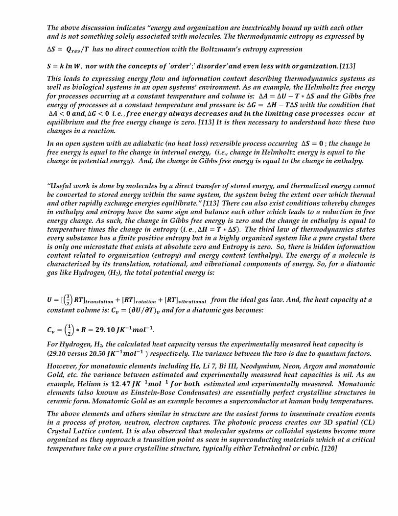
“Useful work is done by molecules by a direct transfer of stored energy, and thermalized energy cannot be converted to stored energy within the same system, the system being the extent over which thermal and other rapidly exchange energies equilibrate.” [113] There can also exist conditions whereby changes in enthalpy and entropy have the same sign and balance each other which leads to a reduction in free energy change. As such, the change in Gibbs free energy is zero and the change in enthalpy is equal to temperature times the change in entropy (𝒊. 𝒆. , ∆𝑯 = 𝑻 ∗ ∆𝑺). The third law of thermodynamics states every substance has a finite positive entropy but in a highly organized system like a pure crystal there is only one microstate that exists at absolute zero and Entropy is zero. So, there is hidden information content related to organization (entropy) and energy content (enthalpy). The energy of a molecule is characterized by its translation, rotational, and vibrational components of energy. So, for a diatomic gas like Hydrogen, (H2), the total potential energy is:
𝑼 = [a𝟑𝟐b𝑹𝑻]𝒕𝒓𝒂𝒏𝒔𝒍𝒂𝒕𝒊𝒐𝒏 + [𝑹𝑻]𝒓𝒐𝒕𝒂𝒕𝒊𝒐𝒏 + [𝑹𝑻]𝒗𝒊𝒃𝒓𝒂𝒕𝒊𝒐𝒏𝒂𝒍 from the ideal gas law. And, the heat capacity at a
constant volume is: 𝑪𝒗 = (𝝏𝑼 𝝏𝑻⁄ )𝒗 and for a diatomic gas becomes: 𝑪𝒗 = v𝟏
𝟐w ∗ 𝑹 = 𝟐𝟗. 𝟏𝟎𝑱𝑲0𝟏𝒎𝒐𝒍0𝟏.
For Hydrogen, H2, the calculated heat capacity versus the experimentally measured heat capacity is (29.10 versus 20.50 𝑱𝑲0𝟏𝒎𝒐𝒍0𝟏) respectively. The variance between the two is due to quantum factors.
However, for monatomic elements including He, Li 7, Bi III, Neodymium, Neon, Argon and monatomic Gold, etc. the variance between estimated and experimentally measured heat capacities is nil. As an example, Helium is 𝟏𝟐. 𝟒𝟕𝑱𝑲0𝟏𝒎𝒐𝒍0𝟏𝒇𝒐𝒓𝒃𝒐𝒕𝒉 estimated and experimentally measured. Monatomic elements (also known as Einstein-Bose Condensates) are essentially perfect crystalline structures in ceramic form. Monatomic Gold as an example becomes a superconductor at human body temperatures.
The above elements and others similar in structure are the easiest forms to inseminate creation events in a process of proton, neutron, electron captures. The photonic process creates our 3D spatial (CL) Crystal Lattice content. It is also observed that molecular systems or colloidal systems become more organized as they approach a transition point as seen in superconducting materials which at a critical temperature take on a pure crystalline structure, typically either Tetrahedral or cubic. [120]
There also exist zones between the Coulomb repulsive forces and the strong force actions which are characterized as Time Reversal Zones (TRZ) where there is a free flow of energy into Negentropy (stored energy) and outward energy flow in Time Forward Zones (TFZ). As an example, the Hydrogen atoms which are positive ions are kept separated by the Coulomb force barrier but when the Hydrogen atoms overcome this barrier the Strong repulsive forces become minimized and the coulomb forces become attractive, (TRZ). It is the Coulomb repulsive force that overcomes the kinetic energy driving hydrogen molecules together. This force becomes so strong that the ions are forced apart or caused to veer . As such, only common chemical reactions occur, (ionic or covalent bonding). This concept appears to elicit a systems approach to understanding both internal forces of the proton and neutron as well as ionic and hydrogen bonding.
Contrary to the above scenario of hydrogen ions forming chemical reactions, in the TRZ the ions of like charge attract and unlike charges repel; an exact opposite of the normal behavior. The Coulomb repulsive force is replaced with a coulomb attractive force and the Strong Force momentarily partially reduced as the gluon forces and fluctuations are greatly reduced. In this TRZ, the quarks in protons and neutrons become weakly bound which is a stark contrast to the normal TFZ.
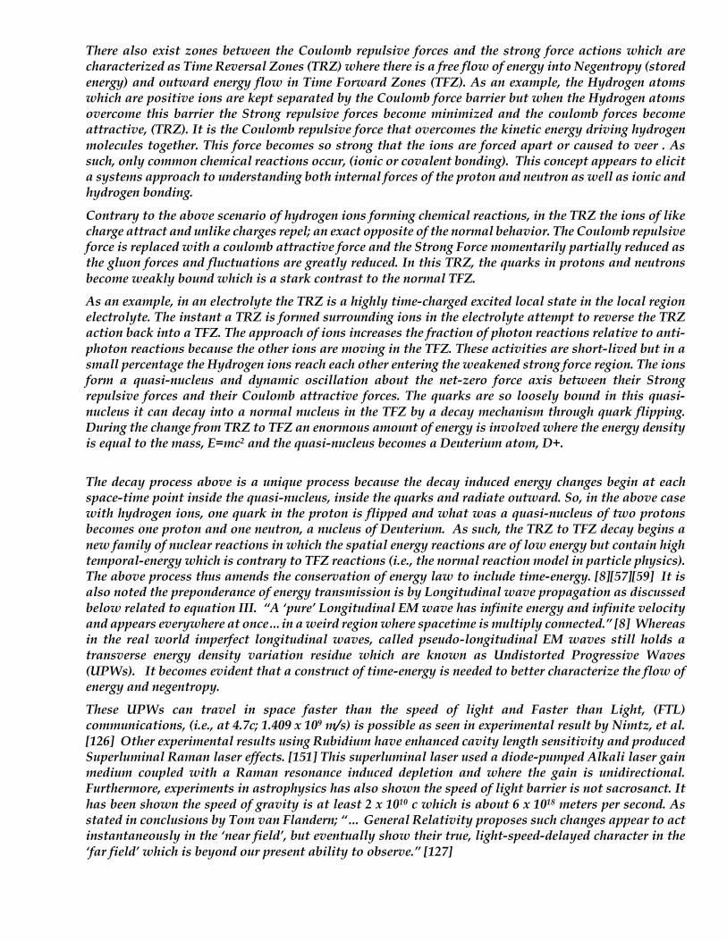
As an example, in an electrolyte the TRZ is a highly time-charged excited local state in the local region electrolyte. The instant a TRZ is formed surrounding ions in the electrolyte attempt to reverse the TRZ action back into a TFZ. The approach of ions increases the fraction of photon reactions relative to anti-photon reactions because the other ions are moving in the TFZ. These activities are short-lived but in a small percentage the Hydrogen ions reach each other entering the weakened strong force region. The ions form a quasi-nucleus and dynamic oscillation about the net-zero force axis between their Strong repulsive forces and their Coulomb attractive forces. The quarks are so loosely bound in this quasi-nucleus it can decay into a normal nucleus in the TFZ by a decay mechanism through quark flipping. During the change from TRZ to TFZ an enormous amount of energy is involved where the energy density is equal to the mass, E=mc2 and the quasi-nucleus becomes a Deuterium atom, D+.
The decay process above is a unique process because the decay induced energy changes begin at each space-time point inside the quasi-nucleus, inside the quarks and radiate outward. So, in the above case with hydrogen ions, one quark in the proton is flipped and what was a quasi-nucleus of two protons becomes one proton and one neutron, a nucleus of Deuterium. As such, the TRZ to TFZ decay begins a new family of nuclear reactions in which the spatial energy reactions are of low energy but contain high temporal-energy which is contrary to TFZ reactions (i.e., the normal reaction model in particle physics). The above process thus amends the conservation of energy law to include time-energy. [8][57][59] It is also noted the preponderance of energy transmission is by Longitudinal wave propagation as discussed below related to equation III. “A ‘pure’ Longitudinal EM wave has infinite energy and infinite velocity and appears everywhere at once…in a weird region where spacetime is multiply connected.” [8] Whereas in the real world imperfect longitudinal waves, called pseudo-longitudinal EM waves still holds a transverse energy density variation residue which are known as Undistorted Progressive Waves (UPWs). It becomes evident that a construct of time-energy is needed to better characterize the flow of energy and negentropy.
These UPWs can travel in space faster than the speed of light and Faster than Light, (FTL) communications, (i.e., at 4.7c; 1.409 x 10⁹ m/s) is possible as seen in experimental result by Nimtz, et al. [126] Other experimental results using Rubidium have enhanced cavity length sensitivity and produced Superluminal Raman laser effects. [151] This superluminal laser used a diode-pumped Alkali laser gain medium coupled with a Raman resonance induced depletion and where the gain is unidirectional. Furthermore, experiments in astrophysics has also shown the speed of light barrier is not sacrosanct. It has been shown the speed of gravity is at least 2 x 10¹⁰ c which is about 6 x 10¹⁸ meters per second. As stated in conclusions by Tom van Flandern; “… General Relativity proposes such changes appear to act instantaneously in the ‘near field’, but eventually show their true, light-speed-delayed character in the ‘far field’ which is beyond our present ability to observe.” [127]
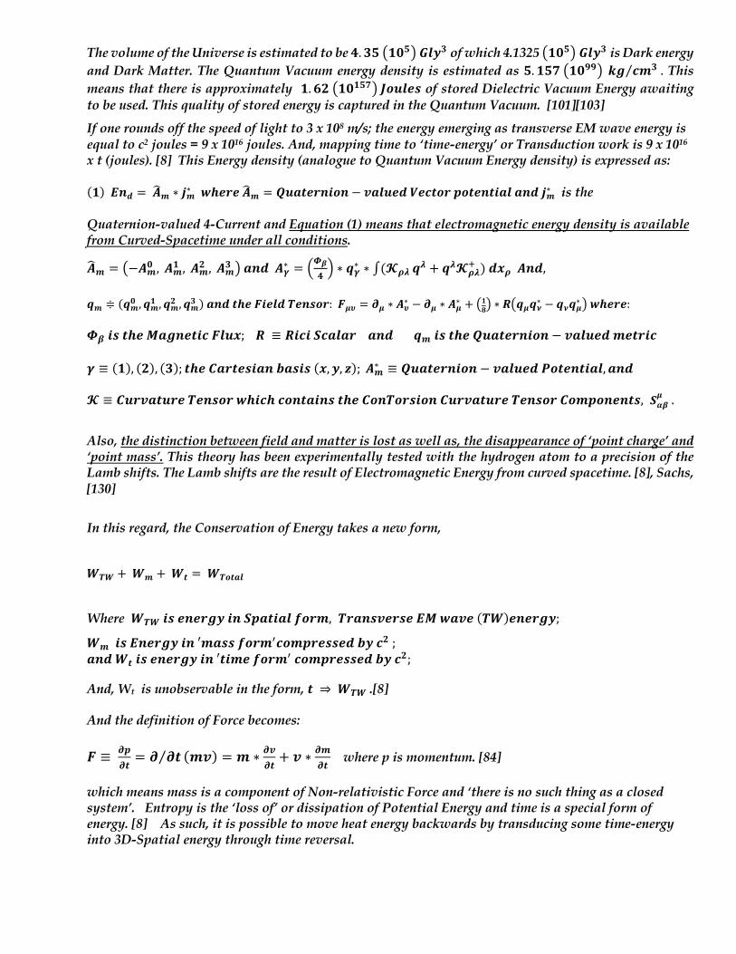
The volume of the Universe is estimated to be 𝟒. 𝟑𝟓L𝟏𝟎𝟓P𝑮𝒍𝒚𝟑of which 4.1325 L𝟏𝟎𝟓P𝑮𝒍𝒚𝟑is Dark energy and Dark Matter. The Quantum Vacuum energy density is estimated as 𝟓. 𝟏𝟓𝟕L𝟏𝟎𝟗𝟗P𝒌𝒈 𝒄𝒎𝟑⁄ . This means that there is approximately 𝟏. 𝟔𝟐L𝟏𝟎𝟏𝟓𝟕P𝑱𝒐𝒖𝒍𝒆𝒔 of stored Dielectric Vacuum Energy awaiting to be used. This quality of stored energy is captured in the Quantum Vacuum. [101][103]
If one rounds off the speed of light to 3 x 10⁸ m/s; the energy emerging as transverse EM wave energy is equal to c2 joules = 9 x 10¹⁶ joules. And, mapping time to ‘time-energy’ or Transduction work is 9 x 10¹⁶ x t (joules). [8] This Energy density (analogue to Quantum Vacuum Energy density) is expressed as: (𝟏)𝑬𝒏𝒅 =𝑨U𝒎 ∗ 𝒋𝒎∗ 𝒘𝒉𝒆𝒓𝒆𝑨U𝒎 = 𝑸𝒖𝒂𝒕𝒆𝒓𝒏𝒊𝒐𝒏 − 𝒗𝒂𝒍𝒖𝒆𝒅𝑽𝒆𝒄𝒕𝒐𝒓𝒑𝒐𝒕𝒆𝒏𝒕𝒊𝒂𝒍𝒂𝒏𝒅𝒋𝒎∗ is the Quaternion-valued 4-Current and Equation (1) means that electromagnetic energy density is available from Curved-Spacetime under all conditions.
𝑨z𝒎 = L−𝑨𝒎𝟎 , 𝑨𝒎𝟏 , 𝑨𝒎𝟐 , 𝑨𝒎𝟑 P𝒂𝒏𝒅𝑨𝜸∗ = v𝜱𝜷𝟒w ∗ 𝒒𝜸∗ ∗ ∫(𝓚𝝆𝝀 𝒒𝝀 + 𝒒𝝀𝓚𝝆𝝀
C )𝒅𝒙𝝆𝑨𝒏𝒅, 𝒒𝒎 ≑ (𝒒𝒎𝟎 , 𝒒𝒎𝟏 , 𝒒𝒎𝟐 , 𝒒𝒎𝟑 )𝒂𝒏𝒅𝒕𝒉𝒆𝑭𝒊𝒆𝒍𝒅𝑻𝒆𝒏𝒔𝒐𝒓:𝑭𝝁𝝊 = 𝝏𝝁 ∗ 𝑨𝝊∗ − 𝝏𝝁 ∗ 𝑨𝝁∗ + k𝟏𝟖l ∗ 𝑹k𝒒𝝁𝒒𝝂
∗ − 𝒒𝝂𝒒𝝁∗ l𝒘𝒉𝒆𝒓𝒆: 𝜱𝜷𝒊𝒔𝒕𝒉𝒆𝑴𝒂𝒈𝒏𝒆𝒕𝒊𝒄𝑭𝒍𝒖𝒙; 𝑹 ≡ 𝑹𝒊𝒄𝒊𝑺𝒄𝒂𝒍𝒂𝒓𝒂𝒏𝒅𝒒𝒎𝒊𝒔𝒕𝒉𝒆𝑸𝒖𝒂𝒕𝒆𝒓𝒏𝒊𝒐𝒏 − 𝒗𝒂𝒍𝒖𝒆𝒅𝒎𝒆𝒕𝒓𝒊𝒄 𝜸 ≡ (𝟏), (𝟐), (𝟑); 𝒕𝒉𝒆𝑪𝒂𝒓𝒕𝒆𝒔𝒊𝒂𝒏𝒃𝒂𝒔𝒊𝒔(𝒙, 𝒚, 𝒛);𝑨𝒎∗ ≡ 𝑸𝒖𝒂𝒕𝒆𝒓𝒏𝒊𝒐𝒏 − 𝒗𝒂𝒍𝒖𝒆𝒅𝑷𝒐𝒕𝒆𝒏𝒕𝒊𝒂𝒍, 𝒂𝒏𝒅 𝓚 ≡ 𝑪𝒖𝒓𝒗𝒂𝒕𝒖𝒓𝒆𝑻𝒆𝒏𝒔𝒐𝒓𝒘𝒉𝒊𝒄𝒉𝒄𝒐𝒏𝒕𝒂𝒊𝒏𝒔𝒕𝒉𝒆𝑪𝒐𝒏𝑻𝒐𝒓𝒔𝒊𝒐𝒏𝑪𝒖𝒓𝒗𝒂𝒕𝒖𝒓𝒆𝑻𝒆𝒏𝒔𝒐𝒓𝑪𝒐𝒎𝒑𝒐𝒏𝒆𝒏𝒕𝒔, 𝑺𝜶𝜷
𝝁 .
Also, the distinction between field and matter is lost as well as, the disappearance of ‘point charge’ and ‘point mass’. This theory has been experimentally tested with the hydrogen atom to a precision of the Lamb shifts. The Lamb shifts are the result of Electromagnetic Energy from curved spacetime. [8], Sachs, [130]
In this regard, the Conservation of Energy takes a new form,
𝑾𝑻𝑾 +𝑾𝒎 +𝑾𝒕 =𝑾𝑻𝒐𝒕𝒂𝒍
Where 𝑾𝑻𝑾𝒊𝒔𝒆𝒏𝒆𝒓𝒈𝒚𝒊𝒏𝑺𝒑𝒂𝒕𝒊𝒂𝒍𝒇𝒐𝒓𝒎, 𝑻𝒓𝒂𝒏𝒔𝒗𝒆𝒓𝒔𝒆𝑬𝑴𝒘𝒂𝒗𝒆(𝑻𝑾)𝒆𝒏𝒆𝒓𝒈𝒚;
𝑾𝒎𝒊𝒔𝑬𝒏𝒆𝒓𝒈𝒚𝒊𝒏′𝒎𝒂𝒔𝒔𝒇𝒐𝒓𝒎F𝒄𝒐𝒎𝒑𝒓𝒆𝒔𝒔𝒆𝒅𝒃𝒚𝒄𝟐; 𝒂𝒏𝒅𝑾𝒕𝒊𝒔𝒆𝒏𝒆𝒓𝒈𝒚𝒊𝒏′𝒕𝒊𝒎𝒆𝒇𝒐𝒓𝒎F𝒄𝒐𝒎𝒑𝒓𝒆𝒔𝒔𝒆𝒅𝒃𝒚𝒄𝟐;
And, Wt is unobservable in the form, 𝒕 ⇒ 𝑾𝑻𝑾.[8] And the definition of Force becomes: 𝑭 ≡ 𝝏𝒑
𝝏𝒕= 𝝏 𝝏𝒕⁄ (𝒎𝒗) = 𝒎 ∗ 𝝏𝒗
𝝏𝒕+ 𝒗 ∗ 𝝏𝒎
𝝏𝒕 where p is momentum. [84]
which means mass is a component of Non-relativistic Force and ‘there is no such thing as a closed system’. Entropy is the ‘loss of’ or dissipation of Potential Energy and time is a special form of energy. [8] As such, it is possible to move heat energy backwards by transducing some time-energy into 3D-Spatial energy through time reversal.

Energy is also stored in biological depots as in plant cells which store photonic energy for Photosynthesis energy used this to convert CO2 into Oxygen and other biomasses. It is also stored energy in living organisms including human cells as ionic bonds between molecules, enzymes and as stored energy for the processing of ADP (Adenodipospahse) into ATP (Adenotriposphase) for use in exoskeletal muscle work. In contrast to the above, the quantity of stored energy in the Earth’s total standing biomass (99% on land, 80% in trees) and an additional amount of dry plant matter, carbon, and produces annually another 60 billion tonnes of carbon and additionally 100 billion in lakes, rivers, and oceans for a grand total of 4664 x L𝟏𝟎𝟏𝟖P𝑱𝒐𝒖𝒍𝒆𝒔, 𝒂𝒃𝒐𝒖𝒕𝟓𝒕𝒐𝟔𝒕𝒊𝒎𝒆𝒔𝒕𝒉𝒆𝒂𝒏𝒏𝒖𝒂𝒍𝒖𝒔𝒂𝒈𝒆.[112] It is also important to remember that these Creation event Conditions are a ‘Snapshot’ in time. The Proton revolution speed is 𝒕𝑷𝒓 = 𝟏. 𝟕𝟔𝟒𝟑𝟔𝟔L𝟏𝟎0𝟐𝟑P𝒔𝒆𝒄𝒐𝒏𝒅𝒔 and this is the typical interaction time given for the Strong force, which is how quickly the Strong Force will capture a particle, (i.e., another Proton or Neutron). Or, also the time an approaching Electron decays (losses Momentum) due to the strong force interaction and is captured in orbit, (Tidal lock).
From Equation (III) above, it is noted there appears two vector wave components, herein described as 𝒌 ∥ 𝒂𝒏𝒅𝒌 ⊥;𝒘𝒉𝒆𝒓𝒆𝒌 ∥ 𝒊𝒔𝒕𝒉𝒆𝒑𝒂𝒓𝒂𝒍𝒍𝒆𝒍𝒍𝒐𝒏𝒈𝒊𝒕𝒖𝒅𝒊𝒏𝒂𝒍𝒘𝒂𝒗𝒆𝒑𝒓𝒐𝒑𝒂𝒈𝒂𝒕𝒊𝒐𝒏(𝒕𝒉𝒆𝒎𝒂𝒋𝒐𝒓𝒄𝒐𝒎𝒑𝒐𝒏𝒆𝒏𝒕)and 𝒌 ⊥ is the perpendicular component (Transient Wave; minor component. The Transient component of the Longitudinal wave is composed of low energy content and short-lived, while the parallel component has a high energy content (time-energy) and portends a much longer propagation characteristic (infinite). An example of this creation event can be evaluated by looking at the ([2,2] H2 ) Hamiltonian of the 2d Euler-Lagrangian Equation which when simplified becomes:
(𝑨)[𝟐, 𝟐]𝓗𝟐 = {ja𝟐𝟓b ∗ 𝜶 ∗ 𝒓𝒎𝒔K ∗ 𝒄 ∗ 𝑹𝒄 ∗ 𝑺𝒆 ∗ 𝒈𝒆 ∗ a
𝟑𝝅𝟐b ∗ a𝝌
𝒏bm ∗ �d�̈�𝓔g𝜱𝓔
𝝐 i + d�̈�𝓔𝝐 g𝜱𝓔i + a
𝟓𝝅𝟏𝟑b ∗ d𝜱𝓔
𝝐 g�̇�𝓔i]�
By examining the 1st Term, we approximate the Energy required in the formation of Lithium 7.
The 1st term becomes: cja𝟐𝟓b ∗ 𝜶 ∗ 𝒓𝒎𝒔K ∗ 𝒄 ∗ 𝑹𝒄 ∗ 𝑺𝒆 ∗ 𝒈𝒆 ∗ a
𝟑𝝅𝟐b ∗ a𝝌
𝒏bm ∗ d�̈�𝓔g𝜱𝓔
𝝐 il and when substituted the Optimal Electron Acceleration for (CL) Lattice Structure creation becomes:
�̈�𝓔 ≈ cja 𝟏𝟓𝟎b ∗ 𝜶 ∗ 𝒓𝒎𝒔K ∗ 𝒄 ∗ 𝑹𝒄 ∗ 𝑺𝒆 ∗ 𝒈𝒆 ∗ a
𝟑𝝅𝟐b ∗ a𝝌
𝒏bm ∗ [𝜱𝓔
𝝐 ]l It is already known that the vibratory energy for Li 7 is about 4 eV. Therefore, the approximate Creation Energy is 200 eV in the Dielectric Vacuum Content at the Space-time point of Li 7 (CL) Lattice Structure creation. This finding is significant in that there exists a methodology for approximating the Periodic Elemental creation process and the required Energies involved. However, this is just a small aspect of the Three-Body model in Space-time.
It is also important to remember the importance of Vibration, Energy and Polarization (i.e., Coherence) which must exist in a harmonic balance to create not only (CL) Lattice structures but also pure crystalline structures for specific purposes. Examples include critical temperatures for phase transitions to create high temperature superconductors, solid state lasers which when pumped with energy (electric or photonic) and bounced back and forth between mirrors coheres into a laser light beam emitted with significantly amplified power over non-coherent light. A 60-watt incandescent light bulb will provide just adequate reading light, whereas a 5-watt laser light will burn one’s retina. Organized energy in vibratory coherence is useful in many applications. Another example is using graphene as a waveguide for Electrons. The wave guide can steer electrons in a 2D graphene valley. This has been accomplished by applying an electrostatic charge across a sheet of single-atom-thick graphene. The device uses carbon Nanotubes atop the sheet of graphene. Scientist believes the device design could work in large circuit networks also enable scientists to create new templates for quantum computing processors which use information stored in the quantum states of electrons. Presently the process is only viable at 1.6 K degrees but it should be able to be reproduced in high temperature superconductors which remain to be designed. [121]
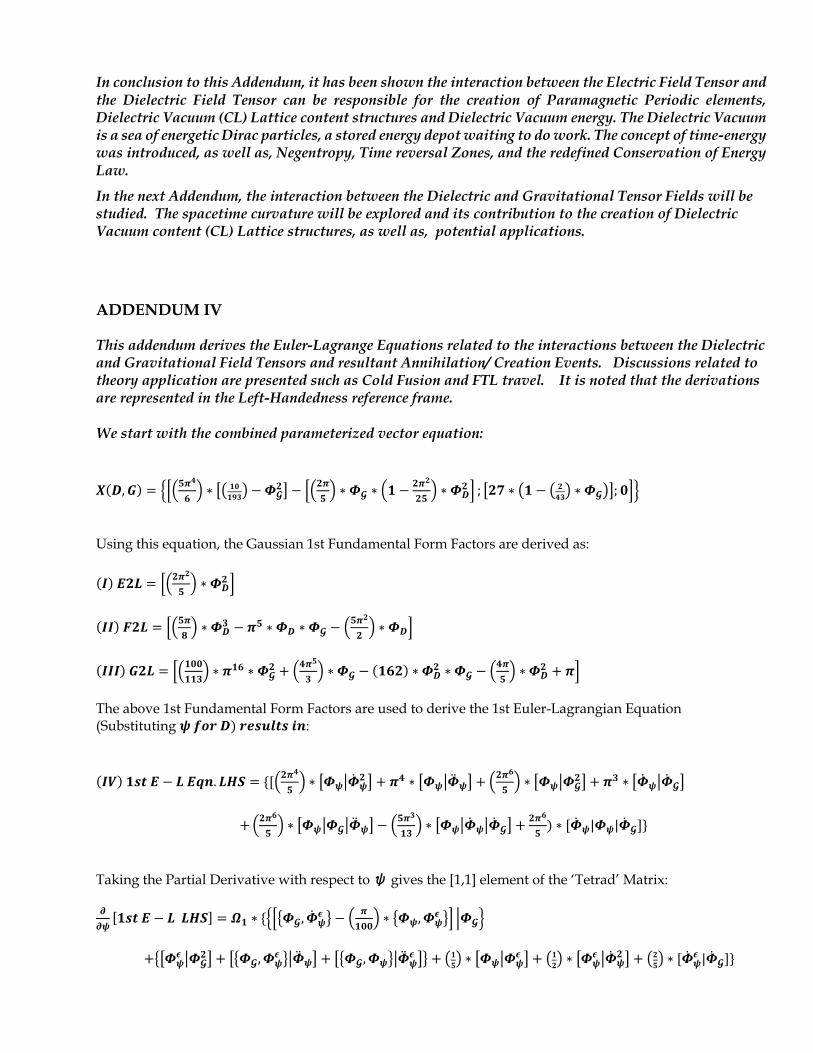
In conclusion to this Addendum, it has been shown the interaction between the Electric Field Tensor and the Dielectric Field Tensor can be responsible for the creation of Paramagnetic Periodic elements, Dielectric Vacuum (CL) Lattice content structures and Dielectric Vacuum energy. The Dielectric Vacuum is a sea of energetic Dirac particles, a stored energy depot waiting to do work. The concept of time-energy was introduced, as well as, Negentropy, Time reversal Zones, and the redefined Conservation of Energy Law.
In the next Addendum, the interaction between the Dielectric and Gravitational Tensor Fields will be studied. The spacetime curvature will be explored and its contribution to the creation of Dielectric Vacuum content (CL) Lattice structures, as well as, potential applications.
ADDENDUM IV This addendum derives the Euler-Lagrange Equations related to the interactions between the Dielectric and Gravitational Field Tensors and resultant Annihilation/ Creation Events. Discussions related to theory application are presented such as Cold Fusion and FTL travel. It is noted that the derivations are represented in the Left-Handedness reference frame. We start with the combined parameterized vector equation:
𝑿(𝑫,𝑮) = cja𝟓𝝅𝟒
𝟔b ∗ d� 𝟏𝟎𝟏𝟗𝟑� − 𝜱𝓖
𝟐i − ja𝟐𝝅𝟓b ∗ 𝜱𝓖 ∗ a𝟏 −
𝟐𝝅𝟐
𝟐𝟓b ∗ 𝜱𝑫
𝟐 m ; d𝟐𝟕 ∗ �𝟏 − � 𝟐𝟒𝟑� ∗ 𝜱𝓖�i; 𝟎ml
Using this equation, the Gaussian 1st Fundamental Form Factors are derived as: (𝑰)𝑬𝟐𝑳 = ja𝟐𝝅
𝟐
𝟓b ∗ 𝜱𝑫
𝟐 m (𝑰𝑰)𝑭𝟐𝑳 = ja𝟓𝝅
𝟖b ∗ 𝜱𝑫
𝟑 − 𝝅𝟓 ∗ 𝜱𝑫 ∗ 𝜱𝓖 − a𝟓𝝅𝟐
𝟐b ∗ 𝜱𝑫m
(𝑰𝑰𝑰)𝑮𝟐𝑳 = ja𝟏𝟎𝟎
𝟏𝟏𝟑b ∗ 𝝅𝟏𝟔 ∗ 𝜱𝓖
𝟐 + a𝟒𝝅𝟓
𝟑b ∗ 𝜱𝓖 − (𝟏𝟔𝟐) ∗ 𝜱𝑫
𝟐 ∗ 𝜱𝓖 − a𝟒𝝅𝟓b ∗ 𝜱𝑫
𝟐 + 𝝅m The above 1st Fundamental Form Factors are used to derive the 1st Euler-Lagrangian Equation (Substituting 𝝍𝒇𝒐𝒓𝑫)𝒓𝒆𝒔𝒖𝒍𝒕𝒔𝒊𝒏:
(𝑰𝑽)𝟏𝒔𝒕𝑬 − 𝑳𝑬𝒒𝒏. 𝑳𝑯𝑺 = {[a𝟐𝝅𝟒
𝟓b ∗ d𝜱𝝍g�̇�𝝍
𝟐 i + 𝝅𝟒 ∗ d𝜱𝝍g�̈�𝝍i + a𝟐𝝅𝟔
𝟓b ∗ d𝜱𝝍g𝜱𝓖
𝟐i + 𝝅𝟑 ∗ d�̇�𝝍g�̇�𝓖i +a𝟐𝝅
𝟔
𝟓b ∗ d𝜱𝝍g𝜱𝓖g�̈�𝝍i − a
𝟓𝝅𝟑
𝟏𝟑b ∗ d𝜱𝝍g�̇�𝝍g�̇�𝓖i +
𝟐𝝅𝟔
𝟓) ∗ [�̇�𝝍|𝜱𝝍|�̇�𝓖]}
Taking the Partial Derivative with respect to ψ gives the [1,1] element of the ‘Tetrad’ Matrix: 𝝏𝝏𝝍[𝟏𝒔𝒕𝑬 − 𝑳𝑳𝑯𝑺] = 𝜴𝟏 ∗ {cje𝜱𝓖, �̇�𝝍
𝝐 f − a 𝝅𝟏𝟎𝟎b ∗ e𝜱𝝍, 𝜱𝝍
𝝐 fm k𝜱𝓖l +ed𝜱𝝍
𝝐 g𝜱𝓖𝟐i + de𝜱𝓖, 𝜱𝝍
𝝐 fg�̈�𝝍i + de𝜱𝓖, 𝜱𝝍fg�̈�𝝍𝝐 if + �𝟏𝟓� ∗ d𝜱𝝍g𝜱𝝍
𝝐 i + �𝟏𝟐� ∗ d𝜱𝝍𝝐 g�̇�𝝍
𝟐 i + �𝟐𝟓� ∗ [�̇�𝝍𝝐 |�̇�𝓖]}

AND, [2,2] is equal to: 𝝏𝝏𝓖[𝟏𝒔𝒕𝑬 − 𝑳𝑳𝑯𝑺] = 𝟐 ∗ 𝜴𝟏 ∗ {d𝜱𝝍g�̇�𝓖
𝝐 i + �𝟏𝟐� ∗ ede𝜱𝓖, �̇�𝝍f − � 𝟑𝟏𝟎𝟎� ∗ e�̇�𝝍, 𝜱𝝍fig�̇�𝓖
𝝐 f +�𝟏𝟐� ∗ de𝜱𝓖
𝝐 , 𝜱𝝍fg�̈�𝝍i + d�𝟏𝟐� ∗ e𝜱𝓖𝝐 , �̇�𝝍fg�̇�𝓖i + � 𝟏𝟐𝟓� ∗ [�̇�𝝍|𝜱𝓖
𝝐 ]}
Since we are now dealing with Left-Handedness the isospin equation becomes:
𝝈² = −𝝈𝟏³ ∗ 𝒆𝟏³−𝝈𝟐³𝒆𝟐³ −𝝈𝟑³𝒆𝟑³𝒘𝒉𝒆𝒓𝒆𝝈²𝟏, 𝝈²𝟐, 𝝈²𝟑𝒂𝒓𝒆𝒕𝒉𝒆𝑷𝒂𝒖𝒍𝒊𝑴𝒂𝒕𝒓𝒊𝒄𝒆𝒔𝒂𝒏𝒅𝒆§𝟏 = [𝟏, 𝟏];𝒆§𝟐 = [𝟐, 𝟐];𝒆§𝟑 = 𝟎
which implies: a𝟎 𝟏𝟏 𝟎b ´
[𝟏, 𝟏] = − � 𝟎[𝟏, 𝟏]� = −𝝈𝟏³ ∗ 𝒆𝟏³a𝟎 −𝒊
𝒊 𝟎 b´[𝟐, 𝟐] = j𝒊 ∗ [𝟐, 𝟐]𝟎 m = −𝝈𝟐³𝒆𝟐³;−𝝈𝟑³𝒆𝟑³ = 𝟎U
This further implies that the Hamiltonian [1,1] is now: [𝟏, 𝟏] = 𝜴𝟏 ∗ {{(𝟕)[O
𝝅𝟏𝟎𝟎P ∗ T𝜱𝝍, 𝜱𝝍
𝝐 V − (𝟖)T𝜱𝓖, �̇�𝝍𝝐 V]|𝜱𝓖
− (𝟗)Te𝜱𝝍𝝐 W𝜱𝓖
𝟐f − (𝟏𝟎)eT𝜱𝓖, 𝜱𝝍𝝐 VW�̈�𝝍f − (𝟏𝟏)eT𝜱𝓖, 𝜱𝝍VW�̈�𝝍
𝝐 fV −(𝟏𝟐)k𝟏𝟓l ∗ M𝜱𝝍N𝜱𝝍
𝝐 Q − (𝟏𝟑)k𝟏𝟐l ∗ M𝜱𝝍𝝐 N�̇�𝝍
𝟐 Q − (𝟏𝟒)k𝟐𝟓l ∗ [�̇�𝝍𝝐 |�̇�𝓖]}
where 𝜴𝟏 = ja𝟑
𝟖b ∗ 𝜶 ∗ 𝒓𝒎𝒔′ ∗ 𝒄 ∗ a𝟑𝝅
𝟐b ∗ 𝑹𝒄 ∗ 𝑺𝒆 ∗ 𝒈𝒆 ∗ a
𝝌𝟐bm [1,1] then becomes:
[𝟏, 𝟏] = 𝜴𝟏 ∗ {{(𝟕) ja𝝅𝟏𝟎𝟎b ∗ e𝜱𝝍, 𝜱𝝍
𝝐 fm g𝜱𝓖 − (𝟖)de𝜱𝓖, �̇�𝝍𝝐 fig𝜱𝓖 − (𝟗)d𝜱𝝍
𝝐 g𝜱𝓖𝟐i − (𝟏𝟎)de𝜱𝓖, 𝜱𝝍
𝝐 fg�̈�𝝍i|�̈�𝝍 −(𝟏𝟏)de𝜱𝓖, 𝜱𝝍fg�̈�𝝍
𝝐 i − (𝟏𝟐)�𝟏𝟓� ∗ d𝜱𝝍g𝜱𝝍𝝐 i − (𝟏𝟑)�𝟏𝟐� ∗ d𝜱𝝍
𝝐 g�̇�𝝍𝟐 i − (𝟏𝟒)�𝟐𝟓� ∗ [�̇�𝝍
𝝐 |�̇�𝓖]}
When the applicable equivalencies from Volume I are substituted, [1,1] becomes:
[𝟏, 𝟏] = 𝜴𝟏 ∗ {(𝟏) J𝝅𝟐K ∗ M�̇�𝓖𝓔
𝝐 N𝜱𝓖𝓔𝟐 Q − (𝟐) q
𝟓𝟏𝟑s ∗ M�̇�𝓖𝑷𝒉
𝝐 N𝜱𝓖𝓔𝟐 Q + (𝟑) q
𝟓𝝅𝟏𝟏s ∗ M�̇�𝓖𝑷𝒉
𝝐 N𝜱𝓖𝑷𝒉𝟐 Q + (𝟒)𝟑 ∗ M�̇�𝓖𝓔
𝝐 N𝜱𝓖𝑷𝒉𝟐 Q
−(𝟓)d𝜱𝓖𝑷𝒉𝝐 g𝜱𝓖𝑷𝒉
𝟐 i − (𝟔)d𝜱𝓖𝓔𝝐 g𝜱𝓖𝓔
𝟐 i − (𝟕)d𝜱𝓖𝑷𝒉𝝐 g𝜱𝓖𝓔
𝟐 i − (𝟖)𝟒 ∗ d𝜱𝓖𝓔g�̇�𝓖𝓔𝝐 g�̈�𝓖𝓔i − (𝟗)𝟒 ∗ d𝜱𝓖𝓔g�̇�𝓖𝓔
𝝐 g�̈�𝓖𝑷𝒉i −(𝟏𝟎)𝟒 ∗ d𝜱𝓖𝓔g�̇�𝓖𝑷𝒉
𝝐 g�̈�𝓖𝓔i − (𝟏𝟏)𝟒 ∗ d𝜱𝓖𝓔g�̇�𝓖𝑷𝒉𝝐 g�̈�𝓖𝓔i − (𝟏𝟐) ∗ d𝜱𝓖𝑷𝒉g𝜱𝓖𝑷𝒉
𝝐 g�̈�𝓖𝑷𝒉i −(𝟏𝟑) a𝟏
𝟓b ∗ d𝜱𝓖𝓔g𝜱𝓖𝓔
𝝐 i − (𝟏𝟒) a𝟏𝟓b ∗ d𝜱𝓖𝑷𝒉g𝜱𝓖𝑷𝒉
𝝐 i
And, [2,2] is composed of Virtual particles = i*[2,2] is defined as:
[𝟐, 𝟐] = 𝜴𝟏 ∗ {[𝟐 ∗ (𝟏){𝒊 ∗ d𝜱𝝍g�̇�𝓖𝝐 i + (𝟐)𝟐 ∗ 𝒊 ∗ a𝟏
𝟐b ∗ ede𝜱𝓖, �̇�𝝍f − (𝟑)𝟐 ∗ 𝒊 ∗ � 𝟑
𝟏𝟎𝟎� ∗ e�̇�𝝍, 𝜱𝝍fig�̇�𝓖𝝐 f
+(𝟒)𝟐 ∗ 𝒊 ∗ �𝟏𝟐� ∗ de𝜱𝓖
𝝐 , 𝜱𝝍fg�̈�𝝍i + (𝟓)𝟐 ∗ d𝒊 ∗ �𝟏𝟐� ∗ e𝜱𝓖𝝐 , �̇�𝝍fg�̇�𝓖i + (𝟔)𝟐 ∗ 𝒊 ∗ � 𝟏𝟐𝟓� ∗ [�̇�𝝍|𝜱𝓖
𝝐 ]]}
Then ∆𝑬 = 𝑬𝟐 − 𝑬𝟏 = {{𝟐[∗ (𝟏)] + [𝟐 ∗ (𝟐)] − [𝟐 ∗ (𝟑)] + [𝟐 ∗ (𝟒)] + [𝟐 ∗ (𝟓)] + [𝟐 ∗ (𝟔)]} − {(𝟕) + (𝟖) + (𝟗) +(10)+(11)+(12)+(13)+(14)}} [2,2] is then expanded by substituting the applicable equivalencies from Volume I, Addendum V, Part A; [2,2] then becomes:
[𝟐, 𝟐] = 𝜴𝟏 ∗ {(𝟏𝟓)𝟐𝒊 ∗ d𝜱𝓖𝓔g�̇�𝓖𝓔
𝝐 i + (𝟏𝟔)𝟐𝒊 ∗ d𝜱𝓖𝑷𝒉g�̇�𝓖𝓔𝝐 i + (𝟏𝟕)𝟐𝒊 ∗ d𝜱𝓖𝓔g𝜱𝓖𝑷𝒉i + (𝟏𝟖)𝟐𝒊 ∗ [𝜱𝓖𝑷𝒉
𝟐 ] +(𝟏𝟗)𝟐𝒊 ∗ d𝜱𝓖𝑷𝒉
𝝐 g�̇�𝓖𝓔𝟐 i + (𝟐𝟎)𝟐𝒊 ∗ d𝜱𝓖𝓔g�̇�𝓖𝓔g�̇�𝓖𝑷𝒉
𝝐 i + (𝟐𝟏)𝟒𝒊 ∗ d𝜱𝓖𝑷𝒉𝝐 g�̇�𝓖𝑷𝒉
𝟐 i − (𝟐𝟐)𝟐𝒊 ∗ d𝜱𝓖𝓔𝟐 g𝜱𝓖𝑷𝒉
𝝐 i −(𝟐𝟑)𝟐𝒊 ∗ d�̇�𝓖𝑷𝒉
𝟐 g𝜱𝓖𝓔𝝐 i + (𝟐𝟒)𝟐𝒊 ∗ d𝜱𝓖𝓔g𝜱𝓖𝑷𝒉g�̇�𝓖𝑷𝒉
𝝐 i In this form all terms in [2,2] would be virtual particles in the Dielectric/ Gravitational interactions in the lower left quadrant 2L or 2L*. However, in modeling with Cartan Geometry the lower left quadrant is rotated to the upper right quadrant with Left-Handedness interpretation and thusly [2,2] is represented as a complete
Hamiltonian Energy and as such ∆𝑬 ≈ 𝑬𝟐 − 𝑬𝟏𝒊𝒔𝒓𝒆𝒑𝒓𝒆𝒔𝒆𝒏𝒕𝒆𝒅𝒃𝒚𝒕𝒉𝒆𝒆𝒙𝒑𝒓𝒆𝒔𝒔𝒊𝒐𝒏:
∆𝑬 =𝜴𝟏 ∗ {𝟐 ∗ d𝜱𝓖𝓔⨂�̇�𝓖𝓔𝝐 i + 𝟐 ∗ d𝜱𝓖𝑷𝒉⨂�̇�𝓖𝓔
𝝐 i + 𝟐 ∗ d𝜱𝓖𝓔⨂𝜱𝓖𝑷𝒉i + 𝟐 ∗ d𝜱𝓖𝑷𝒉𝟐 i + a𝟒𝝅
𝟐
𝟗b ∗ d𝜱𝓖𝑷𝒉
𝝐 ⨂�̇�𝓖𝓔𝟐 i
+𝟐 ∗ d𝜱𝓖𝓔⨂�̇�𝓔⨂�̇�𝓖𝑷𝒉𝝐 i + a𝟒𝝅
𝟓b ∗ d𝜱𝓖𝑷𝒉
𝝐 ⨂𝜱𝓖𝑷𝒉𝟐 i + 𝟑 ∗ d𝜱𝓖𝑷𝒉
𝝐 ⨂𝜱𝓖𝓔𝟐 i − 𝟐 ∗ [d�̇�𝓖𝓔
𝝐 ⨂𝜱𝓖𝑷𝒉𝟐 i
+𝟐 ∗ d𝜱𝓖𝓔⨂𝜱𝓖𝑷𝒉⨂�̇�𝓖𝑷𝒉𝝐 i − a𝝅
𝟐b ∗ d�̇�𝓖𝓔
𝝐 ⨂𝜱𝓖𝓔𝟐 i + d𝜱𝓖𝑷𝒉
𝝐 ⨂𝜱𝓖𝑷𝒉𝟐 i + [𝜱𝓖𝓔
𝝐 ⨂𝜱𝓖𝓔𝟐 ] + 𝟖 ∗ d𝜱𝓖𝓔⨂�̇�𝓖𝓔
𝝐 ⨂�̈�𝓖𝓔i
+𝟖 ∗ d𝜱𝓖𝓔⨂�̇�𝓖𝑷𝒉𝝐 ⨂�̈�𝓖𝓔i + 𝟒 ∗ d𝜱𝓖𝑷𝒉⨂�̇�𝓖𝑷𝒉
𝝐 ⨂�̈�𝓖𝑷𝒉i + a𝟏𝟓b ∗ d𝜱𝓖𝓔⨂𝜱𝓖𝓔
𝝐 i + a𝟏𝟓b ∗ [𝜱𝓖𝑷𝒉⨂𝜱𝓖𝑷𝒉
𝝐 ]}
And the Energy at the Landau-Zener Zero-Line is ∆𝑬 𝟐� which is:
(𝑰)∆𝑬 𝟐� ≈ (𝜴𝟏/𝟐) ∗ {d𝜱𝓖𝓔⨂�̇�𝓖𝓔𝝐 i + d𝜱𝓖𝑷𝒉⨂�̇�𝓖𝓔
𝝐 i + d𝜱𝓖𝓔⨂𝜱𝓖𝑷𝒉i + d𝜱𝓖𝑷𝒉𝟐 i + a𝟐𝝅
𝟐
𝟗b ∗ d𝜱𝓖𝑷𝒉
𝝐 ⨂�̇�𝓖𝓔𝟐 i
+d𝜱𝓖𝓔⨂�̇�𝓔⨂�̇�𝓖𝑷𝒉𝝐 i + a𝟐𝝅
𝟓b ∗ d𝜱𝓖𝑷𝒉
𝝐 ⨂𝜱𝓖𝑷𝒉𝟐 i + d𝜱𝓖𝑷𝒉
𝝐 ⨂𝜱𝓖𝓔𝟐 i − d�̇�𝓖𝓔
𝝐 ⨂𝜱𝓖𝑷𝒉𝟐 i
+M𝜱𝓖𝓔⨂𝜱𝓖𝑷𝒉⨂�̇�𝓖𝑷𝒉𝝐 Q − J𝝅
𝟒K ∗ M�̇�𝓖𝓔
𝝐 ⨂𝜱𝓖𝓔𝟐 Q + k𝟏𝟐l ∗ M𝜱𝓖𝑷𝒉
𝝐 ⨂𝜱𝓖𝑷𝒉𝟐 Q + k𝟏𝟐l ∗ [𝜱𝓖𝓔
𝝐 ⨂𝜱𝓖𝓔𝟐 ] + 𝟒 ∗ M𝜱𝓖𝓔⨂�̇�𝓖𝓔
𝝐 ⨂�̈�𝓖𝓔Q
+𝟒 ∗ M𝜱𝓖𝓔⨂�̇�𝓖𝑷𝒉𝝐 ⨂�̈�𝓖𝓔Q + 𝟐 ∗ M𝜱𝓖𝑷𝒉⨂�̇�𝓖𝑷𝒉
𝝐 ⨂�̈�𝓖𝑷𝒉Q + J𝟏𝟏𝟎K ∗ M𝜱𝓖𝓔⨂𝜱𝓖𝓔
𝝐 Q + J 𝟏𝟏𝟎K ∗ [𝜱𝓖𝑷𝒉⨂𝜱𝓖𝑷𝒉
𝝐 ]} Where 𝜴𝟏 = ja𝟑
𝟖b ∗ 𝜶 ∗ 𝒓𝒎𝒔′ ∗ 𝒄 ∗ a𝟑𝝅
𝟐b ∗ 𝑹𝒄 ∗ 𝑺𝒆 ∗ 𝒈𝒆 ∗ a
𝝌𝟐bm
While expression (I) appears complicated, it is a combination of Annihilation/ Creation Events associated with the Dielectric Vacuum Potential dissipating (i.e., losing inertia/ entropy) and creating Bosons, Photons, Neutrons, Dielectric periodic elements, and curving Spacetime which occur with 99% likelihood. In two examples, the 1st term is an Electron capture event creating Li7 or other Dielectric elements, while the 2d term is an Annihilation event of an Electron producing a Photon(s). For this event(s) to occur the Phase matching frequency, Optimal Electron velocity, and Coulomb/ Strong forces must be ideal. The process is dynamic and occurs on the order of 𝟏𝟎:𝟐𝟑𝒔𝒆𝒄𝒐𝒏𝒅𝒔. It is noted that any production of 𝑯𝟐
Ttakes about the same time in the one-photon and net-two-photon dissociation pathways to stretch to the internuclear distance of the one-photon coupled dipole-transition between the ground and excited electronic states. [131] The theoretical lifetime for an excited state of Hydrogen is: 𝝉 = 𝒕𝒄 𝜶𝟒⁄ = 𝝀𝒄 (𝒄𝜶𝟒)⁄ =𝟐. 𝟖𝟓𝟒𝟎𝟕(𝟏𝟎:𝟏𝟐)𝒔𝒆𝒄𝒐𝒏𝒅𝒔. For heavier atoms this modification may appear stronger and therefore, for elements with more than one electron the mutual orbiting interactions may lead to an increase in lifetimes. [132] Because the Dielectric Vacuum is a dynamic fervent of virtual particles, quarks, bosons, etc., the likelihood is good that such events occur. Additionally, some of the events may be creation of Oriums which decay via electron/ positron annihilation releasing Gamma rays. The above terms are composed of momentum terms, kinetic energy terms, and a combination of kinetic energy/ accelerations.
Next by taking the Partial derivative of (I) with respect to time the expression results in (II):
(𝑰𝑰) 𝝏𝝏𝒕M∆𝑬 𝟐x Q ≈ (𝜴𝟏/𝟐) ∗ {M�̇�𝓖𝓔⨂�̇�𝓖𝓔
𝝐 Q + M𝜱𝓖𝓔⨂�̈�𝓖𝓔𝝐 Q + M�̇�𝓖𝑷𝒉⨂�̇�𝓖𝓔
𝝐 Q + M𝜱𝓖𝑷𝒉⨂�̈�𝓖𝓔𝝐 Q + M�̇�𝓖𝓔⨂𝜱𝓖𝑷𝒉Q + M𝜱𝓖𝓔⨂�̇�𝓖𝑷𝒉Q
+𝟐 ∗ d𝜱𝓖𝑷𝒉⨂�̇�𝓖𝑷𝒉i + a𝟐𝝅𝟐
𝟗b ∗ d�̇�𝓖𝑷𝒉
𝝐 ⨂�̇�𝓖𝓔𝟐 i + a𝟒𝝅
𝟐
𝟗b ∗ d𝜱𝓖𝑷𝒉
𝝐 ⨂�̇�𝓖𝓔⨂�̈�𝓖𝓔i + d�̇�𝓖𝓔⨂�̇�𝓔⨂�̇�𝓖𝑷𝒉𝝐 i
+d𝜱𝓖𝓔⨂�̈�𝓔⨂�̇�𝓖𝑷𝒉𝝐 i + d𝜱𝓖𝓔⨂�̇�𝓔⨂�̈�𝓖𝑷𝒉
𝝐 i + a𝟐𝝅𝟓b ∗ d�̇�𝓖𝑷𝒉
𝝐 ⨂𝜱𝓖𝑷𝒉𝟐 i + a𝟒𝝅
𝟓b ∗ d𝜱𝓖𝑷𝒉
𝝐 ⨂𝜱𝓖𝑷𝒉⨂�̇�𝓖𝑷𝒉i +d�̇�𝓖𝑷𝒉
𝝐 ⨂𝜱𝓖𝓔𝟐 i + 𝟐 ∗ d𝜱𝓖𝑷𝒉
𝝐 ⨂𝜱𝓖𝓔⨂�̇�𝓖𝓔i − d�̈�𝓖𝓔𝝐 ⨂𝜱𝓖𝑷𝒉
𝟐 i − 𝟐 ∗ d�̇�𝓖𝓔𝝐 ⨂𝜱𝓖𝑷𝒉⨂�̇�𝓖𝑷𝒉i + d�̇�𝓖𝓔⨂𝜱𝓖𝑷𝒉⨂�̇�𝓖𝑷𝒉
𝝐 i +M𝜱𝓖𝓔⨂�̇�𝓖𝑷𝒉⨂�̇�𝓖𝑷𝒉
𝝐 Q+ M𝜱𝓖𝓔⨂𝜱𝓖𝑷𝒉⨂�̈�𝓖𝑷𝒉𝝐 Q − J𝝅
𝟒K ∗ M�̈�𝓖𝓔
𝝐 ⨂𝜱𝓖𝓔𝟐 Q − J𝝅
𝟐K ∗ M�̇�𝓖𝓔
𝝐 ⨂𝜱𝓖𝓔⨂�̇�𝓖𝓔Q +k𝟏𝟐l ∗ M�̇�𝓖𝑷𝒉
𝝐 ⨂𝜱𝓖𝑷𝒉𝟐 Q + M𝜱𝓖𝑷𝒉
𝝐 ⨂𝜱𝓖𝑷𝒉⨂�̇�𝓖𝑷𝒉Q + k𝟏𝟐l ∗ M�̇�𝓖𝓔
𝝐 ⨂𝜱𝓖𝓔𝟐 Q + M𝜱𝓖𝓔
𝝐 ⨂𝜱𝓖𝓔⨂�̇�𝓖𝓔Q + 𝟒 ∗ M�̇�𝓖𝓔⨂�̇�𝓖𝓔𝝐 ⨂�̈�𝓖𝓔Q
+𝟒 ∗ j𝜱𝓖𝓔⨂�̈�𝓖𝓔
𝝐 ⨂�̈�𝓖𝓔m + 𝟒 ∗ j𝜱𝓖𝓔⨂�̇�𝓖𝓔
𝝐 ⨂𝜱�𝓖𝓔m + 𝟒 ∗ j�̇�𝓖𝓔⨂�̇�𝓖𝑷𝒉
𝝐 ⨂�̈�𝓖𝓔m + 𝟒 ∗ j𝜱𝓖𝓔⨂�̈�𝓖𝑷𝒉
𝝐 ⨂�̈�𝓖𝓔m +𝟒 ∗ M𝜱𝓖𝓔⨂�̇�𝓖𝑷𝒉
𝝐 ⨂𝜱z𝓖𝓔Q + 𝟐 ∗ M�̇�𝓖𝑷𝒉⨂�̇�𝓖𝑷𝒉𝝐 ⨂�̈�𝓖𝑷𝒉Q + 𝟐 ∗ M𝜱𝓖𝑷𝒉⨂�̈�𝓖𝑷𝒉
𝝐 ⨂�̈�𝓖𝑷𝒉Q + 𝟐 ∗ M𝜱𝓖𝑷𝒉⨂�̇�𝓖𝑷𝒉𝝐 ⨂𝜱z𝓖𝑷𝒉Q
+a 𝟏𝟏𝟎b ∗ j�̇�𝓖𝓔
⨂𝜱𝓖𝓔𝝐 m + a 𝟏
𝟏𝟎b ∗ j𝜱𝓖𝓔
⨂�̇�𝓖𝓔𝝐 m + a 𝟏
𝟏𝟎b ∗ j�̇�𝓖𝑷𝒉
⨂𝜱𝓖𝑷𝒉𝝐 m + a 𝟏
𝟏𝟎b ∗ [𝜱𝓖𝑷𝒉
⨂�̇�𝓖𝑷𝒉𝝐 ]} ≈ [𝜶�] ∗ 𝒕−𝟏
where [𝜶�] is a Constant related to the above terms; collectively as an Energy/time or possibly Time-Energy. It is also noted the 𝜱𝓖𝑷𝒉
𝟐 𝒂𝒏𝒅𝜱𝓖𝓔𝟐 terms are related to the Angular Momentums of the Photon
and Electron, respectively.
The Time-Energy expression II above is composed of Tensor components related to the Dielectric Vacuum Content at the instance in time and the Gravitational Tensor 𝓖𝝁𝝊which is a total Energy-Momentum Stress Tensor which includes the Contorsion Tensor Components for Gravito-Electric and Gravito-Magnetic components described in Volume I . The Contorsion Tensor;
𝓚𝜶𝜷𝝁 ≡ ~−𝑺𝜶𝜷
𝝁 + 𝑺𝜶𝜷𝝁 − 𝑺𝜷𝝁𝜶�𝒂𝒏𝒅𝑺𝒊𝒔𝒂𝒏𝒕𝒊 − 𝒔𝒚𝒎𝒎𝒆𝒕𝒓𝒊𝒄 Torsion Tensor,
𝑺𝜶𝜷𝝁 = 𝟏𝟐 ∗ (𝜞𝑪𝝁𝜶𝜷 − 𝜞𝑪𝝁𝜷𝜶) ; the lower indices are anti-symmetric with the continuity condition satisfied;
(i.e., 𝝏𝒈𝜶𝜷
𝝏𝑪𝝁= 𝟎 = k𝝏𝝁𝒈𝜶𝜷 + 𝜞𝑪l𝒐𝒓 = k𝝏𝝁𝒈𝜶𝜷 − 𝜞𝑪l.
These expressions are also equivalent to specific Spacetime Curvatures which contain Torsion Curvature Components.
And, the Contorsion Tensor is: 𝑺𝜶𝜷𝝁 = M𝑼𝝁 + 𝑺𝜶𝜷Q𝒘𝒉𝒆𝒓𝒆𝑼𝝁𝒊𝒔𝒕𝒉𝒆𝟒 − 𝒗𝒆𝒍𝒐𝒄𝒊𝒕𝒚𝒇𝒊𝒆𝒍𝒅𝒂𝒔𝒔𝒐𝒄𝒊𝒂𝒕𝒆𝒅 with the
Dielectric Vacuum and the ‘S’ terms are Spin-Tensor Density Fields and associated with Gravito-Electrics and Gravito-Magnetics. The Spin-Tensor density fields twist the Helical and create Polarizations (Coherences) which create the (CL) Lattice structures. [47] The Contorsion tensors are analogue to the gravitational forces inside matter which never vanish. Because the Dielectrics are electrically neutral the dipole-moments are invariant and, in the presence of Spin-tensors the Palatini Action implies 𝝏𝝎 ≠ 𝟎𝒔𝒐, 𝝎�𝝁𝒂𝒃 =𝝎𝝁
𝒂𝒃 +𝓚𝝁𝒂𝒃.
The combination of terms in expression (II) above are related to Annihilation/ Creation events occurring at the Landau-Zener Zero-line. While there is a high likelihood of event occurrence at the Zero-line, it is noted that at lesser than Optimal Electron energies (i.e., 3.4 eV, 1.51 eV, etc.), the magnetic radius increases which implies “… at decreased rates of electron rotation its IG fields of the twisted internal RL structure can modulate the surrounding ( CL) lattice space up to a larger radius until the rotating modulation of the circumference reaches the speed of light. Orbiting electrons with optimal or sub-optimal velocities cannot cause external magnetic field beyond some distance from the nucleus. As such, the higher energies in heavier elements come not from a larger electron velocity but from the shrunk (CL) space affected by the accumulated protons and neutrons. This (CL) Space is pumped to higher energy levels in comparison to the (CL) space surrounding the Hydrogen atom. [47]
From the above discussion, it appears three constants, (the Fine Structure, Compton Frequency(or wavelength), and the Rydberg Constant), are embedded in the Electron Structure and its dynamic behavior. The Electron model composes a structure built by sub-elementary particles which are equally involved in the Holographic structure of the (CL) space (physical Vacuum). The Compton frequency dictates the (CL) Node frequency and first proper frequency of the oscillating electron. Additionally, the Compton wavelength dictates the length of the phase propagation of the SPM vector. [132]
Other electron capture events occur creating Dielectric Periodic Elements. The Dielectric Vacuum is a ferment of dynamic interactions. Interactions occur on the order of𝟏𝟎:𝟐𝟑𝒔𝒆𝒄𝒐𝒏𝒅𝒔 with other Neutron/ Proton bombardments creating heavier elements. Whether these interactions create a daughter particle or annihilate releasing photons, positrons or gamma rays is dependent upon the velocity, accelerations, and scattering angles, as well as, coulomb forces and weak forces of the quarks inside the nuclei. While 𝟏𝟎:𝟐𝟑𝒔𝒆𝒄𝒐𝒏𝒅𝒔 appears a brief period, when compared to Planck time (𝟓. 𝟑𝟗𝒙(𝟏𝟎:𝟒𝟒)𝒔𝒆𝒄𝒐𝒏𝒅𝒔 there exists a time period on the order 𝟏𝟎:𝟐𝟎𝒔𝒆𝒄𝒐𝒏𝒅𝒔interval during which Energy (information and energy) may be stored in the Dielectric Vacuum (CL) Lattice structure content. Since there is both conservation of Energy and information, that portion of information and energy not used to create events in the 3D Spatial (CL) Lattice structure content is likely stored in Dark Energy and Dark Matter. It is contained and described by Einstein GR Equation:
𝓖𝝁𝝂 +𝒈𝝁𝝂𝜦 =𝟖𝝅𝑮 𝒄𝟒� ∗𝑻𝝁𝝂 where Λ is the Dielectric Vacuum (CL) Lattice structure content Curvature. The next step is to decompose the Longitudinal propagation wave into its parallel and perpendicular sub-components, where the 𝓓3𝓗∥ 𝒂𝒏𝒅𝓓3𝓗= 𝒂𝒓𝒆𝒗𝒆𝒄𝒕𝒐𝒓𝒔; 𝒕𝒉𝒆𝒇𝒊𝒓𝒔𝒕𝒍𝒚𝒊𝒏𝒈𝒊𝒏𝒕𝒉𝒆𝒂𝒇𝒇𝒊𝒏𝒆𝑻𝒆𝒕𝒓𝒂𝒉𝒆𝒅𝒓𝒐𝒏𝒔𝒖𝒓𝒇𝒂𝒄𝒆𝒂𝒏𝒅𝒕𝒉𝒆𝒔𝒆𝒄𝒐𝒏𝒅 perpendicular to the affine Tetrahedron surface. The perpendicular component is the Poynting Vector.
(𝑨. 𝟏)𝓓3𝓗∥ ≈ 𝜴𝟏 ∗ {(𝟏) J
𝟓𝟏𝟎𝟔K ∗ M�̈�𝓖𝓔
𝝐 ⨂𝜱𝓖𝓔𝟐 Q − (𝟐)k𝟏𝟐l ∗ M𝜱𝓖𝓔
𝟐 ⨂�̈�𝓖𝑷𝒉𝝐 Q + (𝟑)k𝟐𝟕l ∗ M�̈�𝓖𝓔
𝝐 ⨂𝜱𝓖𝑷𝒉𝟐 Q + (𝟒)k𝟐𝟕l ∗ M�̈�𝓖𝑷𝒉⨂𝜱𝓖𝑷𝒉
𝟐 Q +(𝟓)k 𝟓𝟑𝟒l ∗ M𝜱𝓖𝓔
𝟐 ⨂�̈�𝓖𝓔𝝐 ⨂𝜱𝓖𝑷𝒉Q + (𝟔)k
𝟏𝟓l ∗ [𝜱𝓖𝓔
𝟐 ⨂�̈�𝓖𝑷𝒉𝝐 ⨂𝜱𝓖𝑷𝒉]} is the parallel component.
Where, 𝜴𝟏 ≈ L~J 𝟐
𝟏𝟑K ∗ 𝜶 ∗ 𝒓𝒎𝒔′ ∗ 𝒄 ∗ J𝟑𝝅
𝟐K ∗ 𝑹𝒄 ∗ 𝑺𝒆 ∗ 𝒈𝒆 ∗ J
𝝌𝒏K�S
If we equate (A.1) above to the Fusion/ Fission processes involved in Compressed Plasma Fusion reaction (𝑨)𝑷 + 𝑳𝒊𝟑
𝟕 → 𝑩𝒆𝟒𝟖 → 𝟐 𝑯𝒆𝟐
𝟒 + 𝟏𝟖𝑴𝒆𝑽(𝒆𝒙𝒄𝒆𝒔𝒔𝒆𝒏𝒆𝒓𝒈𝒚) then terms (1) -(4) in (A.1) may be associated with Annihilation events and terms (5) and (6) with creation events (i.e., the fusion of the Proton with the LI 7 atoms to form Be 8. If the LHS of (A.1) is equated to the total Binding energy of the proton and Li 7 atom then this is equivalent to 40.2587 MeV. So, we equate: (𝑰𝑽)𝟒𝟎. 𝟐𝟓𝟖𝟕𝑴𝒆𝑽 ≈ 𝜴∗𝟏 ∗ L~𝟐𝟓 ∗ M𝜱𝓖𝓔
𝟐 ⨂�̈�𝓖𝓔𝝐 ⨂𝜱𝓖𝑷𝒉Q + 𝟑𝟒 ∗ M𝜱𝓖𝓔
𝟐 ⨂�̈�𝓖𝑷𝒉𝝐 ⨂𝜱𝓖𝑷𝒉Q�S where 𝜴∗𝟏 = 𝟖𝟑𝒆𝑽 So,
(IV.1) 𝟏𝟒. 𝟐𝟔𝑲𝒆𝑽 ≈ OM𝜱𝓖𝓔
𝟐 ⨂�̈�𝓖𝑷𝒉𝝐 ⨂𝜱𝓖𝑷𝒉Q + (. 𝟕𝟑𝟓) ∗ M𝜱𝓖𝓔
𝟐 ⨂�̈�𝓖𝓔𝝐 ⨂𝜱𝓖𝑷𝒉QP
which means the Fusion portion of (A): 𝑷+ 𝑳𝒊𝟑𝟕 → 𝑩𝒆𝟒
𝟖 releases about 14.26 KeV energy. While, the Annihilation and Fission portion of (A) releases an excess energy of 18 MeV. The energies released from the Fusion and Fission reactions radiate the outside vessel of the reactor which can be converted to direct current using Josephson junctions. Of significance is that the overall process does not irradiate the shell with ionizing radiation nor are the small amount of waste radioactive. [144], [149] If we convert Equation (IV.1) and the RHS results in: 𝟏𝟒. 𝟐𝟔𝑲𝒆𝑽 ≈ 𝟏. 𝟕𝟐𝟑 ∗ OM𝜱𝓖𝓔
𝟐 N𝜱𝓖𝑷𝒉Q�̈�𝓖𝑷𝒉𝝐 + M𝜱𝓖𝓔
𝟐 N�̈�𝓖𝑷𝒉𝝐 Q𝜱𝓖𝑷𝒉P where 𝜱𝓖𝑷𝒉 𝒕𝒆𝒓𝒎𝒔𝒓𝒆𝒑𝒓𝒆𝒔𝒆𝒏𝒕𝑷𝒐𝒔𝒊𝒕𝒓𝒐𝒏𝒔.
This expression means that the Optimal Photon Acceleration for the Fusion process to occur is approximately: �̈�𝓖𝑷𝒉 ≈ 𝟐. 𝟑𝟓𝟑𝟑𝟑(𝟏𝟎E𝟐𝟐)𝒎 𝒔𝟐x
With such a low acceleration, it means that the velocity is constant and is proportionally bound to the Fine structure constant, the Compton frequency (and wavelength), and the Rydberg constant; and optimizes the process when the electron velocity is 13.6 eV or 3.41 eV. This acceleration is also much lower than the Optimal Electron Acceleration derived in Volume I, �̈�𝓔 ≈ 𝟐. 𝟐𝟕𝟑(𝟏𝟎𝟐𝟏)𝒎 𝒔𝟐x .
It is noted that by using the oscillatory qualities of the electron one may create disturbance of the Zero Point Energy (ZPE) waves by means of frequency interaction with the (CL) lattice node Compton frequency. In order to achieve this quantum interaction, Optimal Electron Energies (either 13.6 eV or the 1st subharmonic 3.41 eV) must be maintained so that the electron is phase locked to the phase of the SPM Vector (propagating at light speed). As such, using an alternating electric field (high voltage) with a frequency much lower than the Compton frequency spin flipping can occur as a result of an interaction momentum that occurs between the electron and the (CL) space, (i.e., Physical Vacuum). [47]
What occurs as a result of the Heterodyne Resonance process is a creation of a Neutral Plasma around a properly designed actuator. In the research of Compressed Plasma Fusion, the actuators are finely pointed Nickel cathodes which fire electric discharges into a working medium of Li Hydride and 11% Argon. [141][142][144] In the process, the “ion-electron pairs get reversible motion triggered by a strong electrical field of AC or pulsed DC and a self-sustained by the magnetic field created by the bound electrons.” It is the interaction between the reversible moving electron and the Physical Vacuum that occurs in the moment of spin flipping. This region is referred to by T. Bearden and others (Feynman) as Time Reversal Zones, (TRZ). The Heterodyne Process can be optimized by repeated reactivation and is more effective if the ions in the ion pairs come from an atom with lower atomic mass (such as Lithium 7) in which the magnetic moment of the electron highly predominates the ion magnetic moment. The optimization is dependent upon the selection of the working gas (Lithium Hydride) and a buffer gas, (Argon), the pressure, and the distance between the electrodes . [132][141][144] It is also interesting to note that the term Heterodyne Resonance described above is similar to the Heterodyne damping in the Landau-Zener theorem.
The Transient Wave component, (Poynting Vector) of the propagating Longitudinal Wave is:
(𝑩)𝓓3𝓗= ≈ 𝜴𝟑 ∗ {M�̈�𝓖𝓔𝝐 ⨂𝜱𝓖𝓔
𝟑 Q⨂M𝜱𝓖𝓔𝟐 ⨂�̈�𝓖𝓔⨂𝜱𝓖𝑷𝒉Q + M�̈�𝓖𝓔
𝝐 ⨂𝜱𝓖𝓔𝟑 Q⨂M𝜱𝓖𝓔
𝟐 ⨂�̈�𝓖𝑷𝒉𝝐 ⨂𝜱𝓖𝑷𝒉Q − [�̈�𝓖𝓔
𝝐 ⨂𝜱𝓖𝓔𝟑 ]𝟐
−e�̈�𝓖𝓔𝝐 ⨂𝜱𝓖𝓔
𝟑 f⨂e𝜱𝓖𝓔𝟑 ⨂�̈�𝓖𝑷𝒉
𝝐 f − S 𝟑𝟖𝟓X ∗ e�̈�𝓖𝓔𝝐 ⨂𝜱𝓖𝓔
𝟑 f⨂e𝜱𝓖𝓔𝟑 ⨂𝜱𝓖𝓔
𝝐 f + S 𝟑𝟖𝟓X ∗ [�̈�𝓖𝓔𝝐 ⨂𝜱𝓖𝓔
𝟑 ]⨂[𝜱𝓖𝓔⨂𝜱𝓖𝓔𝝐 ⨂𝜱𝓖𝑷𝒉
𝟐 ] +S 𝟑𝟖𝟓X ∗ e�̈�𝓖𝓔
𝝐 ⨂𝜱𝓖𝓔𝟑 f⨂e𝜱𝓖𝑷𝒉
𝝐 ⨂𝜱𝓖𝑷𝒉𝟑 f + S 𝟑𝟖𝟓X ∗ [�̈�𝓖𝓔
𝝐 ⨂𝜱𝓖𝓔𝟑 ]⨂[𝜱𝓖𝑷𝒉⨂𝜱𝓖𝑷𝒉
𝝐 ⨂𝜱𝓖𝓔𝟐 ]} + [�̈�𝓖𝑷𝒉
𝝐 ⨂𝜱𝓖𝓔𝟑 ]⨂[𝜱𝓖𝓔
𝟐 ⨂�̈�𝓖𝓔𝝐 ⨂𝜱𝓖𝑷𝒉]
+e�̈�𝓖𝑷𝒉𝝐 ⨂𝜱𝓖𝓔
𝟑 f⨂e𝜱𝓖𝓔𝟐 ⨂�̈�𝓖𝑷𝒉
𝝐 ⨂𝜱𝓖𝑷𝒉f − e�̈�𝓖𝑷𝒉𝝐 ⨂𝜱𝓖𝓔
𝟑 f⨂e�̈�𝓖𝓔𝝐 ⨂𝜱𝓖𝓔
𝟑 f − [�̈�𝓖𝑷𝒉𝝐 ⨂𝜱𝓖𝓔
𝟑 ]⨂[𝜱𝓖𝓔𝟑 ⨂�̈�𝓖𝑷𝒉
𝝐 ] −S 𝟑𝟖𝟓X ∗ e�̈�𝓖𝑷𝒉
𝝐 ⨂𝜱𝓖𝓔𝟑 f⨂e𝜱𝓖𝓔
𝟑 ⨂𝜱𝓖𝓔𝝐 f + S 𝟑𝟖𝟓X ∗ e�̈�𝓖𝑷𝒉
𝝐 ⨂𝜱𝓖𝓔𝟑 f⨂e𝜱𝓖𝓔⨂𝜱𝓖𝓔
𝝐 ⨂𝜱𝓖𝑷𝒉𝟐 f + S 𝟑𝟖𝟓X ∗ e�̈�𝓖𝑷𝒉
𝝐 ⨂𝜱𝓖𝓔𝟑 f⨂e𝜱𝓖𝑷𝒉
𝝐 ⨂𝜱𝓖𝑷𝒉𝟑 f
+S 𝟑𝟖𝟓X ∗ e�̈�𝓖𝑷𝒉𝝐 ⨂𝜱𝓖𝓔
𝟑 f⨂e𝜱𝓖𝑷𝒉⨂𝜱𝓖𝑷𝒉𝝐 ⨂𝜱𝓖𝓔
𝟐 f + e�̈�𝓖𝓔𝝐 ⨂𝜱𝓖𝑷𝒉
𝟑 f⨂e𝜱𝓖𝓔𝟐 ⨂�̈�𝓖𝓔
𝝐 ⨂𝜱𝓖𝑷𝒉f + e�̈�𝓖𝓔𝝐 ⨂𝜱𝓖𝑷𝒉
𝟑 fe𝜱𝓖𝓔𝟐 ⨂�̈�𝓖𝑷𝒉
𝝐 ⨂𝜱𝓖𝑷𝒉f −e�̈�𝓖𝓔
𝝐 ⨂𝜱𝓖𝑷𝒉𝟑 f⨂e�̈�𝓖𝓔
𝝐 ⨂𝜱𝓖𝓔𝟑 f − e�̈�𝓖𝓔
𝝐 ⨂𝜱𝓖𝑷𝒉𝟑 fe𝜱𝓖𝓔
𝟑 ⨂�̈�𝓖𝑷𝒉𝝐 f − S 𝟑𝟖𝟓X ∗ e�̈�𝓖𝓔
𝝐 ⨂𝜱𝓖𝑷𝒉𝟑 f⨂e𝜱𝓖𝓔
𝟑 ⨂𝜱𝓖𝓔𝝐 f
+I 𝟑𝟖𝟓J ∗ K�̈�𝓖𝓔𝝐 ⨂𝜱𝓖𝑷𝒉
𝟑 N⨂K𝜱𝓖𝓔⨂𝜱𝓖𝓔𝝐 ⨂𝜱𝓖𝑷𝒉
𝟐 N + I 𝟑𝟖𝟓J ∗ K�̈�𝓖𝓔𝝐 ⨂𝜱𝓖𝑷𝒉
𝟑 N⨂K𝜱𝓖𝑷𝒉𝝐 ⨂𝜱𝓖𝑷𝒉
𝟑 N + I 𝟑𝟖𝟓J ∗ K�̈�𝓖𝓔𝝐 ⨂𝜱𝓖𝑷𝒉
𝟑 N⨂K𝜱𝓖𝑷𝒉⨂𝜱𝓖𝑷𝒉𝝐 ⨂𝜱𝓖𝓔
𝟐 N +e�̈�𝓖𝑷𝒉⨂𝜱𝓖𝑷𝒉
𝟑 f⨂e𝜱𝓖𝓔𝟐 ⨂�̈�𝓖𝓔
𝝐 ⨂𝜱𝓖𝑷𝒉f + e�̈�𝓖𝑷𝒉⨂𝜱𝓖𝑷𝒉𝟑 f⨂e𝜱𝓖𝓔
𝟐 ⨂�̈�𝓖𝑷𝒉𝝐 ⨂𝜱𝓖𝑷𝒉f − [�̈�𝓖𝑷𝒉⨂𝜱𝓖𝑷𝒉
𝟑 ]⨂e�̈�𝓖𝓔𝝐 ⨂𝜱𝓖𝓔
𝟑 f −e�̈�𝓖𝑷𝒉⨂𝜱𝓖𝑷𝒉
𝟑 f⨂e𝜱𝓖𝓔𝟑 ⨂�̈�𝓖𝑷𝒉
𝝐 f − S 𝟑𝟖𝟓X ∗ e�̈�𝓖𝑷𝒉⨂𝜱𝓖𝑷𝒉𝟑 f⨂e𝜱𝓖𝓔
𝟑 ⨂𝜱𝓖𝓔𝝐 f + S 𝟑𝟖𝟓X ∗ e�̈�𝓖𝑷𝒉⨂𝜱𝓖𝑷𝒉
𝟑 f⨂e𝜱𝓖𝓔⨂𝜱𝓖𝓔𝝐 ⨂𝜱𝓖𝑷𝒉
𝟐 f +S 𝟑𝟖𝟓X ∗ e�̈�𝓖𝑷𝒉⨂𝜱𝓖𝑷𝒉
𝟑 f⨂e𝜱𝓖𝑷𝒉𝝐 ⨂𝜱𝓖𝑷𝒉
𝟑 f + S 𝟑𝟖𝟓X ∗ [�̈�𝓖𝑷𝒉⨂𝜱𝓖𝑷𝒉𝟑 ]⨂[𝜱𝓖𝑷𝒉⨂𝜱𝓖𝑷𝒉
𝝐 ⨂𝜱𝓖𝓔𝟐 ]}
Where, 𝜴𝟑 ≈ {RS 𝟏𝟏𝟕X ∗ 𝜶 ∗ 𝒓𝒎𝒔′ ∗ 𝒄 ∗ O𝟓𝝅
𝟐P ∗ 𝑹𝒄 ∗ 𝑺𝒆 ∗ 𝒈𝒆 ∗ O
𝝌𝟐P[}
Note that even though Expression (B) has many more terms than (A), the wave propagation is short lived compared to the Parallel Wave Propagation expression (A). Expression (A) is the Longitudinal wave propagation form which contains various components as Scalar Waves, (UPWs) Undistorted Progressive Waves, etc. Additionally, because we are at a sub-harmonic (lesser than Optimal Electron energy) the Magnetic Flux Energy is greater and can by Torsion (i.e., curvature of Spacetime) effect the micro-structure, (Figure 4.1) of Addendum IV, Volume I.[46]-[49] As a result, there exists a high likelihood that Positrons are created from Electron Annihilations. “… When an Electron moves through space, it is actually swimming in a sea of ghost particles of all varieties--virtual leptons, quarks, and messengers, entangled in a complex 𝒎𝒆§𝒍�́�𝒆. The Electron will distort this irreducible vacuum activity, and the distortion in turn reacts back on
the electron.” [84] Note also that all terms in the (A) 𝓓U𝓗∥ are related to momentums, acceleration, and mass sub-components. As such, there is an isometry between the Longitudinal planar wave form, its amplitude, and momentums, as well as, the correlation to the Tetrahedral CL Lattice Structural content which is a result of the proton sub-nucleonic structure and quark isospin dynamics.
“In General Relativity, if there is mass or charge anywhere in the universe, then the whole of spacetime is curved, and all the laws of physics must be written in Curved Spacetime, including, of course, the laws of Electrodynamics. Regarded in this light, the O(3) electrodynamics of Evans and the homomorphic SU(2) electrodynamics of Barrett are written correctly in Conformally Curved Spacetime and are cases of Einstein’s general relativity as developed by Sachs. …Flat spacetime (as assumed in classical U(1) electrodynamics) as the description of the vacuum is valid only when the whole Universe is empty.” [130]
In a more modern view of Force, Mass must exist in the vacuum of space; 𝑭 ≡ 𝝏𝒑 𝝏𝒕⁄ and p is momentum. “The force field in space” idea was a basic premise of Maxwellian assumption about material ‘ether’. All Forces of Nature are generated by the interaction of virtual particle flux upon observable mass and charge and as such generated by a precursor. “…The virtual partial flux with its dynamic, (its associated curved spacetime dynamics [and torsions]) is a causative precursor to force and field. …Once the forces are generated, the changes caused by the forces to the observable mass and observable charge are measurable, but not the causative virtual particle flux dynamics themselves.” These virtual particle flux dynamics are the “Incommensurate” Content of the Dielectric Vacuum. “Only effects are observed, not primary causes.” [84] This last fact is why Dark Matter/ Dark Energy is mapped across the universe by observation of Baryonic Resonance fluctuations. The virtual particle flux (Incommensurate) can be directly engineered and manipulated before they interact with charged mass by a force-free manipulation of their precursors by means of ‘re-gauging’. Re-gauging can be used to create useful work with minor energy furnished by the operator. “… the fundamental result of Differential geometry implies that electromagnetic energy cab be transmitted from a source to a receiver by Scalar curvature, R, and that electromagnetic energy is available in non-Euclidean spacetime,”…” the Charge obtainable from a given Curvature R in a given volume is about twelve orders of magnitude greater than the mass obtainable from the same curvature R for the same volume.” “…Electromagnetic Energy from non-Euclidean spacetime is available to the earth-bound engineer in usable form, and originates in the curvatures inherent in the rest of the Universe,” M. Evans, [25]
The question arises, “HOW” does one ‘re-gauge’ to “effect” a desired change upon the mass and charge? Since we already know that: 𝑭𝝁𝝂𝑭𝝁𝝂 = [𝑬𝟐 −𝑩𝟐]𝒂𝒏𝒅𝑭𝝁𝝂 = 𝝏𝝁𝑨𝝂∗ − 𝝏𝝁𝑨𝝁∗ +
𝜱𝜷
𝟖𝑹�𝒒𝝁𝒒𝝂∗ − 𝒒𝝂𝒒𝝁∗ � it appears
that we need to change the electric field (High Voltage); not necessarily high Amperage, and changing the magnetic field by oscillatory pulsing.
In further experiments in LENR (Compressed Plasma), it has been established the byproduct produced by pulsed dense plasma is the creation of EVOs (Exotic Vacuum Objects) which have a Negative Resistance (E-Cat Tests). In these experiments, Lithium Hydroxide mixed with an 11 % concentration of Argon gas is pulsed with an electric arc from a finely pointed Nickel cathode. The result is an EVO which starts a sequence of nuclear reactions between Hydrogen and Lithium:
(𝑨)𝑷 + 𝑳𝒊𝟑𝟕 → 𝑩𝒆𝟒
𝟖 → 𝟐 𝑯𝒆𝟐𝟒 + 𝟏𝟖𝑴𝒆𝑽(𝒆𝒙𝒄𝒆𝒔𝒔𝒆𝒏𝒆𝒓𝒈𝒚)
“In the first step, Hydrogen and Lithium atoms, merge exothermically, overcoming the Coulomb electrostatic barrier where the short-range strong nuclear prevail, and transmuting (via fusion) into a highly excited state. In the second step, the excited Beryllium undergoes exothermic fission by splitting into: 𝑩𝒆𝟒𝟖 𝒂𝒏𝒅𝒕𝒘𝒐 𝑯𝒆𝟐
𝟒 𝒂𝒕𝒐𝒎𝒔, 𝒔𝒐 − 𝒄𝒂𝒍𝒍𝒆𝒅𝒂𝒍𝒑𝒉𝒂𝒓𝒂𝒅𝒊𝒂𝒕𝒊𝒐𝒏𝒔,𝒘𝒉𝒊𝒄𝒉𝒂𝒓𝒆𝒂𝒃𝒔𝒐𝒓𝒃𝒆𝒅𝒃𝒚𝒕𝒉𝒆𝒓𝒆𝒂𝒄𝒕𝒐𝒓𝒘𝒂𝒍𝒍𝒔 and contribute globally to the yield of high thermal energy, WITHOUT ionizing radiations. The energy produced is Orders of magnitude greater than any chemical energies from the same substances. [139]

The Energy efficiency surpasses any other energy source and is comparable to nuclear fission reactions. It is estimated the U.S. Navy’s patent: US20190295733A1, “Plasma Compression Fusion Device”; which is of small size (.3-2 meters) can produce between 1 Giga-Watt and 1 Terra-Watt of power which far exceeds the largest Nuclear reactor (Palo Verde, AZ) 3 Giga-watt plant on 4,000 acres. The patent application states this technology is “Operable”, not theory. [142]
The underlying theme and characteristics that evolve from the prior discussions, addendum, theory, and supporting references is the sub-structures of matter are related to both cubic crystal and tetrahedral lattice structures; the Hamiltonians are expressive of both the propagating planar wave amplitudes; and the sub-nucleonic structures can be expressed geometrically in a cubic lattice. The Dielectric Vacuum (CL) Lattice structure is geometrically modeled with Planckian Tetrahedral holographic structure for the Proton inter-nucleonic dynamics and is quantal entangled with the rest of the universe. The Holographic Dielectric Vacuum content may be visualized as a quantum network of these connected Planckian Holographic Tetrahedrons where the vertices' connection points of the dihedral angles are the Quantum (CL) Lattice Nodes (QLNs). The QLNs are analogue to what Leibniz in the 1600s described as “Monads” which are the smallest constituent of the Quantum CL Spacetime and which contain a Cosmic consciousness. These QLNs are quantum entangled with all other QLNs in the Cosmic Quantum CL Spacetime content. Each of the sides of the quantum network tetrahedrons form Micro-wormholes that connect all other QLNs and can transmit information at speeds greater than 10,000 times the speed of light, c, essentially instantaneously. The Tetrahedrons form multiple CL Lattice prism structures of which the Face Centered Cubic Crystal is a sub-harmonic isometry.
The Dielectric Vacuum is an Incommensurate composed of a fervent dynamic of virtual particles, leptons, bosons, baryons, etc. which are in an ever-increasing creation process contributing to the universal expansion. While the Spatial (CL) Lattice structure content may be modeled geometrically with the Cubic crystalline lattice structure, the face centered cubic structure contains tetrahedron structures for hydrogen and hydrogen bonds. Living organisms contain a high percentage of water which act like liquid crystals in a tetrahedral lattice which is quantal entangled with brain neurons which can instantaneously sense the organism’s reactions to heat/ cold/ taste, smell, touch, etc. The sub-structure of the nucleus/ electron can be manipulated by means of pulsed magnetic oscillations which when properly attuned to the specific frequency and pulse rate can produce significant results including high-powered lasers, compressed plasma fusion to anti-Gravitics, FTL (faster-than-light) communications [151] and travel, as well as, plentiful energy transmitted wirelessly and room temperature super-conductors. The world is on the verge of emerging from the ‘Energy Dark Ages’.
Briefing leaving the Longitudinal Plane Wave (LW) (A) and carrying forward the concept of ‘Re-gauging’ to effectuate a change to the Spacetime Energy-Momentum Stresses and Spacetime Curvature, it is seen that for the conditions of a particle slowing moving in weak gravitational field the nonlinear terms in Einstein’s Field Equations become a set of Gravito-Magnetic type gravity equations:
(𝟏)𝜵 ∙ 𝒈 = −𝟒𝝅𝑮𝝆 (𝟐)𝜵 ∙ 𝓚 = 𝟎
(𝟑)𝜵⨂𝒈 = 𝟎 q𝜵⨂𝒈 = −𝝏𝓚𝝏𝒕 s
(𝟒)𝜵⨂𝓚 = −J𝟒𝝅𝒄K ∗ (𝟒𝑮𝝆𝝂) + 𝟒
𝒄𝝏𝒈𝝏𝒕
And, (𝟓)𝑭 = 𝒆 ∗ J𝑬 + 𝝂⨂𝑩
𝒄K +𝒎 ∗ ~𝒈 + 𝝂⨂𝓚
𝒄� + ~𝒎𝝂
𝟐𝒄𝝏𝝋𝝏𝒕� 𝒘𝒉𝒆𝒓𝒆𝑮𝒊𝒔𝒕𝒉𝒆𝒈𝒓𝒂𝒗𝒊𝒕𝒂𝒕𝒊𝒐𝒏𝒂𝒍𝒄𝒐𝒏𝒔𝒕𝒂𝒏𝒕𝒂𝒏𝒅
𝒈 ≡ 𝑮𝒓𝒂𝒗𝒊𝒕𝒚𝑭𝒊𝒆𝒍𝒅, 𝓚𝒊𝒔𝒕𝒉𝒆𝑪𝒐 − 𝑮𝒓𝒂𝒗𝒊𝒕𝒂𝒕𝒊𝒐𝒏𝒂𝒍𝑭𝒊𝒆𝒍𝒅(𝒐𝒓𝑮𝒓𝒂𝒗𝒊𝒕𝒐 −𝑴𝒂𝒈𝒏𝒆𝒕𝒊𝒄𝑭𝒊𝒆𝒍𝒅)𝒔𝒐𝒎𝒆𝒕𝒊𝒎𝒆𝒔𝒓𝒆𝒇𝒆𝒓𝒓𝒆𝒅𝒂𝒔𝑯𝒊, 𝒂𝒏𝒅𝝆𝒊𝒔𝒎𝒂𝒔𝒔𝒅𝒆𝒏𝒔𝒊𝒕𝒚,𝒂𝒏𝒅𝝋𝒊𝒔𝒕𝒉𝒆𝑺𝒄𝒂𝒍𝒂𝒓𝑷𝒐𝒕𝒆𝒏𝒕𝒊𝒂𝒍𝒐𝒇𝒕𝒉𝒆𝑬𝒍𝒆𝒄𝒕𝒓𝒐 −𝑴𝒂𝒈𝒏𝒆𝒕𝒊𝒄𝑭𝒊𝒆𝒍𝒅. [𝟏𝟑𝟓]
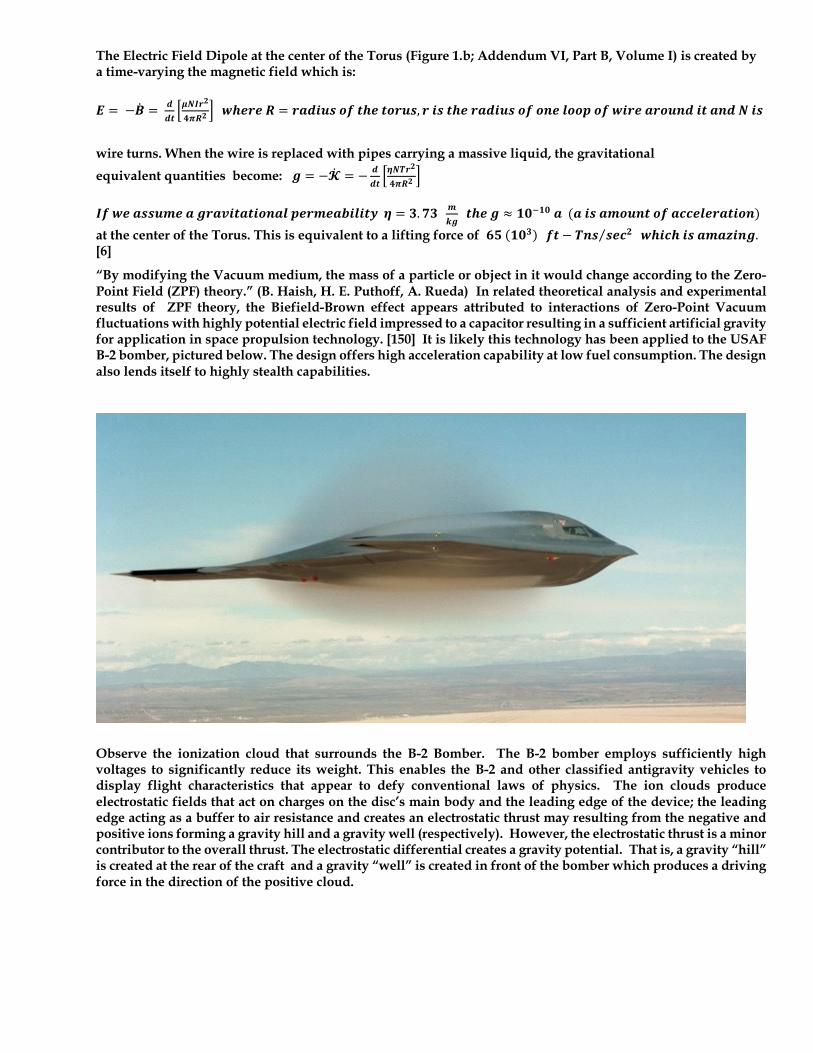
The Electric Field Dipole at the center of the Torus (Figure 1.b; Addendum VI, Part B, Volume I) is created by a time-varying the magnetic field which is: 𝑬 =−�̇� = 𝒅
𝒅𝒕~𝝁𝑵𝑰𝒓
𝟐
𝟒𝝅𝑹𝟐� 𝒘𝒉𝒆𝒓𝒆𝑹 = 𝒓𝒂𝒅𝒊𝒖𝒔𝒐𝒇𝒕𝒉𝒆𝒕𝒐𝒓𝒖𝒔, 𝒓𝒊𝒔𝒕𝒉𝒆𝒓𝒂𝒅𝒊𝒖𝒔𝒐𝒇𝒐𝒏𝒆𝒍𝒐𝒐𝒑𝒐𝒇𝒘𝒊𝒓𝒆𝒂𝒓𝒐𝒖𝒏𝒅𝒊𝒕𝒂𝒏𝒅𝑵𝒊𝒔
wire turns. When the wire is replaced with pipes carrying a massive liquid, the gravitational equivalent quantities become: 𝒈 = −�̇� = − 𝒅
𝒅𝒕~𝜼𝑵𝑻𝒓
𝟐
𝟒𝝅𝑹𝟐�
𝑰𝒇𝒘𝒆𝒂𝒔𝒔𝒖𝒎𝒆𝒂𝒈𝒓𝒂𝒗𝒊𝒕𝒂𝒕𝒊𝒐𝒏𝒂𝒍𝒑𝒆𝒓𝒎𝒆𝒂𝒃𝒊𝒍𝒊𝒕𝒚𝜼 = 𝟑. 𝟕𝟑 𝒎
𝒌𝒈𝒕𝒉𝒆𝒈 ≈ 𝟏𝟎E𝟏𝟎𝒂(𝒂𝒊𝒔𝒂𝒎𝒐𝒖𝒏𝒕𝒐𝒇𝒂𝒄𝒄𝒆𝒍𝒆𝒓𝒂𝒕𝒊𝒐𝒏)
at the center of the Torus. This is equivalent to a lifting force of 𝟔𝟓(𝟏𝟎𝟑)𝒇𝒕 − 𝑻𝒏𝒔 𝒔𝒆𝒄𝟐⁄ 𝒘𝒉𝒊𝒄𝒉𝒊𝒔𝒂𝒎𝒂𝒛𝒊𝒏𝒈. [6]
“By modifying the Vacuum medium, the mass of a particle or object in it would change according to the Zero-Point Field (ZPF) theory.” (B. Haish, H. E. Puthoff, A. Rueda) In related theoretical analysis and experimental results of ZPF theory, the Biefield-Brown effect appears attributed to interactions of Zero-Point Vacuum fluctuations with highly potential electric field impressed to a capacitor resulting in a sufficient artificial gravity for application in space propulsion technology. [150] It is likely this technology has been applied to the USAF B-2 bomber, pictured below. The design offers high acceleration capability at low fuel consumption. The design also lends itself to highly stealth capabilities.
Observe the ionization cloud that surrounds the B-2 Bomber. The B-2 bomber employs sufficiently high voltages to significantly reduce its weight. This enables the B-2 and other classified antigravity vehicles to display flight characteristics that appear to defy conventional laws of physics. The ion clouds produce electrostatic fields that act on charges on the disc’s main body and the leading edge of the device; the leading edge acting as a buffer to air resistance and creates an electrostatic thrust may resulting from the negative and positive ions forming a gravity hill and a gravity well (respectively). However, the electrostatic thrust is a minor contributor to the overall thrust. The electrostatic differential creates a gravity potential. That is, a gravity “hill” is created at the rear of the craft and a gravity “well” is created in front of the bomber which produces a driving force in the direction of the positive cloud.
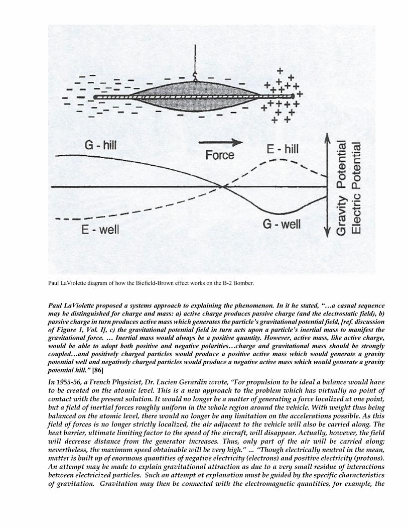
Paul LaViolette diagram of how the Biefield-Brown effect works on the B-2 Bomber.
Paul LaViolette proposed a systems approach to explaining the phenomenon. In it he stated, “…a casual sequence may be distinguished for charge and mass: a) active charge produces passive charge (and the electrostatic field), b) passive charge in turn produces active mass which generates the particle’s gravitational potential field, [ref. discussion of Figure 1, Vol. I], c) the gravitational potential field in turn acts upon a particle’s inertial mass to manifest the gravitational force. … Inertial mass would always be a positive quantity. However, active mass, like active charge, would be able to adopt both positive and negative polarities…charge and gravitational mass should be strongly coupled…and positively charged particles would produce a positive active mass which would generate a gravity potential well and negatively charged particles would produce a negative active mass which would generate a gravity potential hill.” [86]
In 1955-56, a French Physicist, Dr. Lucien Gerardin wrote, “For propulsion to be ideal a balance would have to be created on the atomic level. This is a new approach to the problem which has virtually no point of contact with the present solution. It would no longer be a matter of generating a force localized at one point, but a field of inertial forces roughly uniform in the whole region around the vehicle. With weight thus being balanced on the atomic level, there would no longer be any limitation on the accelerations possible. As this field of forces is no longer strictly localized, the air adjacent to the vehicle will also be carried along. The heat barrier, ultimate limiting factor to the speed of the aircraft, will disappear. Actually, however, the field will decrease distance from the generator increases. Thus, only part of the air will be carried along; nevertheless, the maximum speed obtainable will be very high.” … “Though electrically neutral in the mean, matter is built up of enormous quantities of negative electricity (electrons) and positive electricity (protons). An attempt may be made to explain gravitational attraction as due to a very small residue of interactions between electricized particles. Such an attempt at explanation must be guided by the specific characteristics of gravitation. Gravitation may then be connected with the electromagnetic quantities, for example, the
multi-polar moments in the nuclei. It is thus clear that knowledge of the nature of gravitational forces is closely connected with the nature of the atomic nucleus.” [176]
In the Theory of Basic Structures of Matter-Supergravitation Unified Theory, (BSM-SG), the Stimulated Anomalous Reaction of Gravity (SARG) effect is activated by a Heterodyne Resonance Method which invokes Quantum Mechanical interactions between the oscillating ion-electron pairs and the Spacetime continuum. The theory shows the relation between forces in Nature while premising: Empty Euclidean space; two fundamental particles of super dense matter with vibratory frequencies at the Planck range; and a fundamental law of Super-Gravity which holds that forces between FPs is: 𝑭𝑺𝑮 =
𝑮 ∗ 𝑴𝟏 ∗ 𝒎𝟐𝑹𝟑� . The
Theory leads from a self-organized process in supermassive astronomical object to Crystallization of Sub-elemental particles (twisted prisms) which are embedded in elementary particles known as Cosmic Lattice or Crystal Lattice (CL) structure with quantum properties. The connected points in the CL structure are called CL Nodes which are flexible and composed of four identical prisms. These CL Nodes are comprised of two reference frames of symmetrical axes, one orthogonal (xyz) and one aligned along the major axes of the prisms (abcd) and the distance between CL Nodes is about 𝟏. 𝟎𝟗𝟕(𝟏𝟎:𝟐𝟎)𝒎. It has been found through experiments that the return SG forces (define the CL stiffness) along the abcd axes are thousands of times stronger than the forces along the xyz axes and this permits 3D oscillations of the CL Node. Analysis shows these oscillations are composed of two cycles, a resonance cycle of 𝑽𝑹 = 𝟏. 𝟎𝟗𝟐𝟔(𝟏𝟎𝟐𝟗)𝑯𝒛 and a Spatial Precessional Momentum with a frequency equivalent to the Compton frequency of 𝟏. 𝟐𝟑𝟔(𝟏𝟎𝟐𝟎)𝑯𝒛. “The static and dynamic properties of the CL Nodes permit understanding of the physical relation between gravity and inertia and electrical and magnetic fields (EM and light) on the other side.” [154][See also 86] It is also relevant that Anti-matter such as Antiprotons have been shown to repulse matter rather than attract. [157] By applying the electron structure developed in [44], the key parameters of the CL Space are:
𝑺𝒕𝒂𝒕𝒊𝒄𝑷𝒓𝒆𝒔𝒔𝒖𝒓𝒆:𝑷𝑺 =𝒎𝒆 ∗𝒄𝟐
𝑽𝒆= 𝟏. 𝟑𝟕𝟑𝟔(𝟏𝟎𝟐𝟔)𝑵 𝒎𝟐�
𝑫𝒚𝒏𝒂𝒎𝒊𝒄𝑷𝒓𝒆𝒔𝒔𝒖𝒓𝒆:𝑷𝑫 =𝒉𝝂𝒄
𝒄 ∗ 𝑺𝒆� = 𝟐𝟎𝟐𝟓. 𝟖 j𝑵 𝒎𝟐𝑯𝒛� m And,
𝑷𝒂𝒓𝒕𝒊𝒂𝒍𝑪𝑳𝑷𝒓𝒆𝒔𝒔𝒖𝒓𝒆:𝑷𝑷 =𝑷𝑺 ∗ 𝜶 ∗ 𝝊 𝒄⁄ 𝒇𝒐𝒓𝝊 = 𝜶 ∗ 𝒄: 𝑷𝑷 𝑷𝑺⁄ = 𝜶𝟐 ∗ (𝟏 − 𝜶)3𝟏𝟐
Where: 𝒄 = 𝒍𝒊𝒈𝒉𝒕𝒔𝒑𝒆𝒆𝒅;𝒎𝒆 − 𝒆𝒍𝒆𝒄𝒕𝒓𝒐𝒏𝒎𝒂𝒔𝒔;𝑽𝒆 − 𝑰𝒎𝒑𝒆𝒏𝒆𝒕𝒓𝒂𝒃𝒍𝒆𝑽𝒐𝒍𝒖𝒎𝒆𝒐𝒇𝒕𝒉𝒆𝑬𝒍𝒆𝒄𝒕𝒓𝒐𝒏; 𝜶 −𝑭𝒊𝒏𝒆𝑺𝒕𝒓𝒖𝒄𝒕𝒖𝒓𝒆𝑪𝒐𝒏𝒔𝒕𝒂𝒏𝒕;𝑺𝒆 − 𝒔𝒖𝒓𝒇𝒂𝒄𝒆𝒐𝒇𝒕𝒉𝒆𝒆𝒍𝒆𝒄𝒕𝒓𝒐𝒏𝒔𝒕𝒓𝒖𝒄𝒕𝒖𝒓𝒆, 𝒉 − 𝑷𝒍𝒂𝒏𝒄𝒌𝒄𝒐𝒏𝒔𝒕𝒂𝒏𝒕; 𝝊 −𝒆𝒍𝒆𝒄𝒕𝒓𝒐𝒏𝒗𝒆𝒍𝒐𝒄𝒊𝒕𝒚; 𝒂𝒏𝒅𝝂𝒄 − 𝑪𝒐𝒎𝒑𝒕𝒐𝒏𝒇𝒓𝒆𝒒𝒖𝒆𝒏𝒄𝒚 − 𝟏. 𝟐𝟑𝟔(𝟏𝟎𝟐𝟎)𝑯𝒛
The Static Pressure defines the Newtonian mass as a pressure exercised on the elementary particle structure and the Dynamic (CL) Pressure defines the ZPE of dynamic type and is responsible for the Electrical and Magnetic Fields. The stable mass equation for an elementary particle with impenetrable volume VH is derived from the static pressure and the electron structure:
𝒎 = a𝑷𝑺 𝒄𝟐� b ∗ 𝑽𝑯 = �𝟐𝒉𝝂𝒄𝟒 ∗ (𝟏 − 𝜶𝟐)
𝝅 ∗ 𝜶𝟐 ∗ 𝒄𝟓½ � ∗ 𝑽𝒆 This equation shows the mass of a particle/ object can be changed by changing the Static Pressure of the RHS . To do so, the light speed of the RHS must be changed by Superhigh Compton frequency through proper Quantum Mechanical interaction.[154] Therefore, the self-synchronization of the CL Space may be asymmetrically disturbed around a material object (particle, atom, molecule, etc.) creating a Gravitational sink into which the object will fall. [“falling is following.” K. Wheeler.] In other words, by affecting the Compton frequency and changing the static pressure the Spacetime Curvature is effectuated and an Alcubierre affect may be created which portends Travel at FTL.
The search for Dark Matter and Energy has proven to be a formidable task. Since Dark Energy and Dark Matter represent weakly interactive particles and energy, it remains necessary to formulate a method of tapping into this Energy repository for use in doing work. One such method is the Boudini MEG, (Motionless Electric Generator) which utilizes Time-Energy and Time-Reversal Zones (TRZs) to generate energy for work purposes. [84] Other devices including the Searle energy generator also so promise. Other developments in Compressed Plasma Fusion reactors holds great promise for immense energy output for minor energy and fuel input.
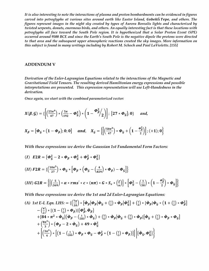
It is also interesting to note the interactions of plasma and proton bombardments can be evidenced in figures carved into petroglyphs at various sites around earth like Easter Island, 𝑮𝒐𝒃𝒆𝒌𝒍¾𝑻𝒆𝒑𝒆̈ , and others. The figures represent images in the night sky created by types of Aurora Borealis lights and characterized by twisted serpents, donuts, enormous birds, and others. An equally interesting fact is that these locations with petroglyphs all face toward the South Pole region. It is hypothesized that a Solar Proton Event (SPE) occurred around 9500 BCE and since the Earth’s South Pole is the negative dipole the protons were directed to that area and the subsequent upper atmospheric reactions created the sky images. More information on this subject is found in many writings including by Robert M. Schoch and Paul LaViolette. [155]
ADDENDUM V
Derivation of the Euler-Lagrangian Equations related to the interactions of the Magnetic and Gravitational Field Tensors. The resulting derived Hamiltonian energy expressions and possible interpretations are presented. This expression representation will use Left-Handedness in the derivation.
Once again, we start with the combined parameterized vector:
𝑿(𝜷, 𝓖) = {c:𝟐𝟓𝝅𝟒
𝟒𝟕; ∗ : 𝟓𝝅
𝟏𝟗𝟐−𝜱𝓖
𝟐; ∗ d𝟏 −𝜱𝜷𝟐
𝟐f gh ;=𝟐𝟕 ∗ 𝜱𝓖D; 𝟎} and,
𝑿𝜷 = =𝜱𝓖 ∗ j𝟏 − 𝜱𝜷k; 𝟎; 𝟎D𝒂𝒏𝒅,𝑿𝓖 = op:𝟓𝟎𝝅𝟒
𝟒𝟕; ∗ 𝜱𝓖 + q𝟏 −
𝜱𝜷𝟐
𝟐rs ; (+𝟏); 𝟎t
With these expressions we derive the Gaussian 1st Fundamental Form Factors: (𝑰)𝑬𝟐𝑹 = >𝜱𝓖
𝟐 − 𝟐 ∗ 𝜱𝜷 ∗ 𝜱𝓖𝟐 +𝜱𝜷
𝟐 ∗ 𝜱𝓖𝟐?
(𝑰𝑰)𝑭𝟐𝑹 = {:𝟏𝟎𝝅
𝟓
𝟐𝟕; ∗ 𝜱𝓖 ∗ F𝜱𝜷 ∗ :𝜱𝓖 − :
𝟒𝟖𝟐𝟗; ∗ 𝜱𝜷) − 𝜱𝓖IH
(𝑰𝑰𝑰)𝑮𝟐𝑹 = oF: 𝟓𝟑𝟔𝟗; ∗ 𝜶 ∗ 𝒓𝒎𝒔′ ∗ 𝒄 ∗ (𝒏𝝅) ∗ 𝑮 ∗ 𝑺𝒆 ∗ :
𝝌𝒏;I ∗ p𝜱𝓖
𝟐 − : 𝟏𝟓𝟎; ∗ q𝟏 −
𝜱𝜷𝟐
𝟐r ∗ 𝜱𝓖st
With these expressions we derive the 1st and 2d Euler-Lagrangian Equations:
(A) 1st E-L Eqn. LHS: = {:𝟕𝝅𝟏𝟎; ∗ =�̇�𝜷@𝜱𝜷@�̇�𝓖 + j𝟏𝟐k ∗ �̇�𝜷@�̇�𝓖
𝟐D + j𝟏𝟒k ∗ [�̇�𝜷|�̇�𝓖 ∗ j𝟏 + j𝟏𝟐k ∗ 𝜱𝜷𝟐 D
−:𝝅𝟐; ∗ [(𝟏 − j𝟏𝟐k ∗ 𝜱𝜷)|>𝜱𝜷
𝟐 , �̈�𝜷? +[𝟖𝟒 ∗ 𝝅𝟐 ∗ �̇�𝓖@j�̇�𝜷 − j 𝟏
𝟏𝟎𝟎k ∗ �̇�𝓖k + j𝟓𝟔k ∗ �̇�𝜷@�̇�𝓖 + j𝟓𝟗k ∗ �̇�𝜷|=�̇�𝓖 + j𝟏𝟐k ∗ �̇�𝜷 ∗ 𝜱𝓖D
+:𝟖𝝅𝟓
𝟑; ∗ j𝜱𝜷 − 𝟐 ∗ �̇�𝓖k + 𝟒𝟗 ∗ �̇�𝓖
𝟐
+ c:𝟑𝝅𝟑
𝟒; ∗ Fj𝟏 − j 𝟏
𝟐𝟎𝟎k ∗ 𝜱𝜷 ∗ 𝜱𝓖 −𝜱𝜷𝟐 ∗ j𝟏 − j𝟏𝟐k ∗ 𝜱𝜷kDI y>�̈�𝓖, 𝜱𝓖
𝟐?z
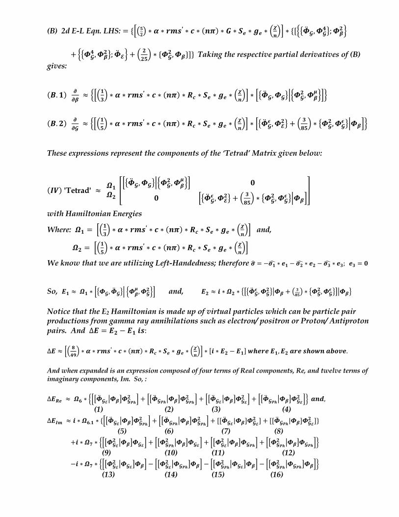
(B) 2d E-L Eqn. LHS: = {Fj𝟓𝟐k ∗ 𝜶 ∗ 𝒓𝒎𝒔′ ∗ 𝒄 ∗ (𝒏𝝅) ∗ 𝑮 ∗ 𝑺𝒆 ∗ 𝒈𝒆 ∗ :
𝝌𝒏;I ∗ {[<>�̈�𝓖, 𝜱𝓖
𝟒?;𝜱𝜷𝟐H
+<>𝜱𝓖
𝟒 , 𝜱𝜷𝟐?; �̈�𝓔H + :
𝟐𝟐𝟓; ∗ {𝜱𝓖
𝟐 , 𝜱𝜷}]}Taking the respective partial derivatives of (B) gives:
(𝑩. 𝟏) 𝝏𝝏𝜷≈ <F:𝟏
𝟑; ∗ 𝜶 ∗ 𝒓𝒎𝒔′ ∗ 𝒄 ∗ (𝒏𝝅) ∗ 𝑹𝒄 ∗ 𝑺𝒆 ∗ 𝒈𝒆 ∗ :
𝝌𝒏;I ∗ F>�̈�𝓖, 𝜱𝓖?G<𝜱𝓖
𝟐 , 𝜱𝜷𝝁HIH
(𝑩. 𝟐) 𝝏
𝝏𝓖≈ <F:𝟏
𝟓; ∗ 𝜶 ∗ 𝒓𝒎𝒔′ ∗ 𝒄 ∗ (𝒏𝝅) ∗ 𝑹𝒄 ∗ 𝑺𝒆 ∗ 𝒈𝒆 ∗ :
𝝌𝒏;I ∗ F>�̈�𝓖
𝝐 , 𝜱𝓔𝟐? + : 𝟑
𝟖𝟓; ∗ >𝜱𝓖
𝟐 , 𝜱𝓖𝝐 ?G𝜱𝜷IH
These expressions represent the components of the ‘Tetrad’ Matrix given below:
(𝑰𝑽) 'Tetrad' ≈𝜴𝟏𝜴𝟐~F>�̈�𝓖, 𝜱𝓖?G<𝜱𝓖
𝟐 , 𝜱𝜷𝝁HI 𝟎
𝟎 F>�̈�𝓖𝝐 , 𝜱𝓔
𝟐? + : 𝟑𝟖𝟓; ∗ >𝜱𝓖
𝟐 , 𝜱𝓖𝝐 ?G𝜱𝜷I
�
with Hamiltonian Energies
Where: 𝜴𝟏 = F:𝟏𝟑; ∗ 𝜶 ∗ 𝒓𝒎𝒔′ ∗ 𝒄 ∗ (𝒏𝝅) ∗ 𝑹𝒄 ∗ 𝑺𝒆 ∗ 𝒈𝒆 ∗ :
𝝌𝒏;I and,
𝜴𝟐 = F:𝟏𝟓; ∗ 𝜶 ∗ 𝒓𝒎𝒔′ ∗ 𝒄 ∗ (𝒏𝝅) ∗ 𝑹𝒄 ∗ 𝑺𝒆 ∗ 𝒈𝒆 ∗ :
𝝌𝒏;I
We know that we are utilizing Left-Handedness; therefore 𝝈� = −𝝈𝟏� ∗ 𝒆𝟏 − 𝝈𝟐� ∗ 𝒆𝟐 − 𝝈𝟑� ∗ 𝒆𝟑; 𝒆𝟑 = 𝟎
So, 𝑬𝟏 ≈𝜴𝟏 ∗ je𝜱𝓖, �̈�𝓖fk c𝜱𝜷𝝁 , 𝜱𝓖
𝟐lm and, 𝑬𝟐 ≈ 𝒊 ∗ 𝜴𝟐 ∗ ede�̈�𝓖𝝐 , 𝜱𝓖
𝟐fg𝜱𝜷 + � 𝟑𝟖𝟓� ∗ e𝜱𝓖𝟐 , 𝜱𝓖
𝝐 fig𝜱𝜷f Notice that the E2 Hamiltonian is made up of virtual particles which can be particle pair productions from gamma ray annihilations such as electron/ positron or Proton/ Antiproton pairs. And ∆𝑬 = 𝑬𝟐 − 𝑬𝟏𝒊𝒔: ∆𝑬 ≈ ja 𝟖
𝟒𝟗b ∗ 𝜶 ∗ 𝒓𝒎𝒔′ ∗ 𝒄 ∗ (𝒏𝝅) ∗ 𝑹𝒄 ∗ 𝑺𝒆 ∗ 𝒈𝒆 ∗ a
𝝌𝒏bm ∗ [𝒊 ∗ 𝑬𝟐 − 𝑬𝟏]𝒘𝒉𝒆𝒓𝒆𝑬𝟏, 𝑬𝟐𝒂𝒓𝒆𝒔𝒉𝒐𝒘𝒏𝒂𝒃𝒐𝒗𝒆.
And when expanded is an expression composed of four terms of Real components, Re, and twelve terms of imaginary components, Im. So, : ∆𝑬𝑹𝒆 ≈ 𝜴𝟔 ∗ cjd�̈�𝓖𝓔g𝜱𝜷i𝜱𝓖𝑷𝒉
𝟐 m + jd�̈�𝓖𝑷𝒉g𝜱𝜷i𝜱𝓖𝑷𝒉𝟐 m + jd�̈�𝓖𝓔g𝜱𝜷i𝜱𝓖𝓔
𝟐 m + jd�̈�𝓖𝑷𝒉g𝜱𝜷i𝜱𝓖𝓔𝟐 ml 𝒂𝒏𝒅,
(1) (2) (3) (4) ∆𝑬𝑰𝒎 ≈ 𝒊 ∗ 𝜴𝟔.𝟏 ∗ {jd�̈�𝓖𝓔g𝜱𝜷i𝜱𝓖𝑷𝒉
𝟐 m + jd�̈�𝓖𝑷𝒉g𝜱𝜷i𝜱𝓖𝑷𝒉𝟐 m + [[�̈�𝓖𝓔|𝜱𝜷]𝜱𝓖𝓔
𝟐 ] + [[�̈�𝓖𝑷𝒉|𝜱𝜷]𝜱𝓖𝓔𝟐 ]}
(5) (6) (7) (8) +𝒊 ∗ 𝜴𝟕 ∗ cjd𝜱𝓖𝓔
𝟐 g𝜱𝜷i𝜱𝓖𝓔m + jd𝜱𝓖𝑷𝒉𝟐 g𝜱𝜷i𝜱𝓖𝓔m + jd𝜱𝓖𝓔
𝟐 g𝜱𝜷i𝜱𝓖𝑷𝒉m + jd𝜱𝓖𝑷𝒉𝟐 g𝜱𝜷i𝜱𝓖𝑷𝒉ml
(9) (10) (11) (12) −𝒊 ∗ 𝜴𝟕 ∗ cjd𝜱𝓖𝓔
𝟐 g𝜱𝓖𝓔i𝜱𝜷m − jd𝜱𝓖𝓔𝟐 g𝜱𝓖𝑷𝒉i𝜱𝜷m − jd𝜱𝓖𝑷𝒉
𝟐 g𝜱𝓖𝓔i𝜱𝜷m − jd𝜱𝓖𝑷𝒉𝟐 g𝜱𝓖𝑷𝒉i𝜱𝜷ml
(13) (14) (15) (16)
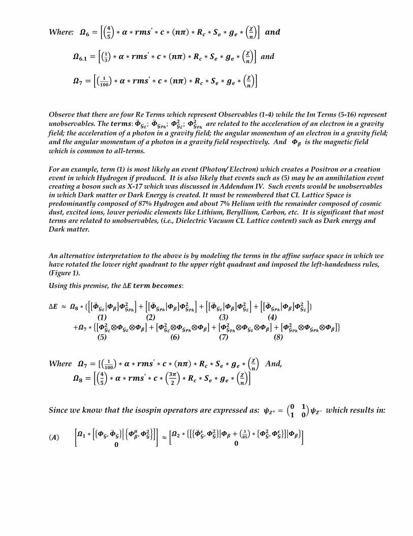
Where: 𝜴𝟔 = F:𝟒𝟓; ∗ 𝜶 ∗ 𝒓𝒎𝒔′ ∗ 𝒄 ∗ (𝒏𝝅) ∗ 𝑹𝒄 ∗ 𝑺𝒆 ∗ 𝒈𝒆 ∗ :
𝝌𝒏;I 𝒂𝒏𝒅
𝜴𝟔.𝟏 = Fj𝟏𝟑k ∗ 𝜶 ∗ 𝒓𝒎𝒔
′ ∗ 𝒄 ∗ (𝒏𝝅) ∗ 𝑹𝒄 ∗ 𝑺𝒆 ∗ 𝒈𝒆 ∗ :𝝌𝒏;I and
𝜴𝟕 = Fj 𝟏
𝟏𝟎𝟎k ∗ 𝜶 ∗ 𝒓𝒎𝒔′ ∗ 𝒄 ∗ (𝒏𝝅) ∗ 𝑹𝒄 ∗ 𝑺𝒆 ∗ 𝒈𝒆 ∗ :
𝝌𝒏;I
Observe that there are four Re Terms which represent Observables (1-4) while the Im Terms (5-16) represent unobservables. The 𝒕𝒆𝒓𝒎𝒔:�̈�𝓖𝓔; �̈�𝓖𝑷𝒉; 𝜱𝓖𝓔
𝟐 ; 𝜱𝓖𝑷𝒉𝟐 are related to the acceleration of an electron in a gravity
field; the acceleration of a photon in a gravity field; the angular momentum of an electron in a gravity field; and the angular momentum of a photon in a gravity field respectively. And 𝜱𝜷 is the magnetic field which is common to all-terms. For an example, term (1) is most likely an event (Photon/ Electron) which creates a Positron or a creation event in which Hydrogen if produced. It is also likely that events such as (5) may be an annihilation event creating a boson such as X-17 which was discussed in Addendum IV. Such events would be unobservables in which Dark matter or Dark Energy is created. It must be remembered that CL Lattice Space is predominantly composed of 87% Hydrogen and about 7% Helium with the remainder composed of cosmic dust, excited ions, lower periodic elements like Lithium, Beryllium, Carbon, etc. It is significant that most terms are related to unobservables, (i.e., Dielectric Vacuum CL Lattice content) such as Dark energy and Dark matter. An alternative interpretation to the above is by modeling the terms in the affine surface space in which we have rotated the lower right quadrant to the upper right quadrant and imposed the left-handedness rules, (Figure 1).
Using this premise, the ∆𝑬𝒕𝒆𝒓𝒎𝒃𝒆𝒄𝒐𝒎𝒆𝒔: ∆𝑬 ≈ 𝜴𝟖 ∗ {jd�̈�𝓖𝓔g𝜱𝜷i𝜱𝓖𝑷𝒉
𝟐 m + jd�̈�𝓖𝑷𝒉g𝜱𝜷i𝜱𝓖𝑷𝒉𝟐 m + jd�̈�𝓖𝓔g𝜱𝜷i𝜱𝓖𝓔
𝟐 m + jd�̈�𝓖𝑷𝒉g𝜱𝜷i𝜱𝓖𝓔𝟐 m}
(1) (2) (3) (4) +𝜴𝟕 ∗ ed𝜱𝓖𝓔
𝟐 ⨂𝜱𝓖𝓔⨂𝜱𝜷i + d𝜱𝓖𝓔𝟐 ⨂𝜱𝓖𝑷𝒉⨂𝜱𝜷i + d𝜱𝓖𝑷𝒉
𝟐 ⨂𝜱𝓖𝓔⨂𝜱𝜷i + d𝜱𝓖𝑷𝒉𝟐 ⨂𝜱𝓖𝑷𝒉⨂𝜱𝜷if
(5) (6) (7) (8)
Where 𝜴𝟕 = [j 𝟏𝟏𝟎𝟎k ∗ 𝜶 ∗ 𝒓𝒎𝒔
′ ∗ 𝒄 ∗ (𝒏𝝅) ∗ 𝑹𝒄 ∗ 𝑺𝒆 ∗ 𝒈𝒆 ∗ :𝝌𝒏; And,
𝜴𝟖 = F:𝟒𝟓; ∗ 𝜶 ∗ 𝒓𝒎𝒔′ ∗ 𝒄 ∗ :𝟑𝝅
𝟐; ∗ 𝑹𝒄 ∗ 𝑺𝒆 ∗ 𝒈𝒆 ∗ :
𝝌𝒏;I
Since we know that the isospin operators are expressed as: 𝝍𝒁2 =a𝟎 𝟏𝟏 𝟎b𝝍𝒁3 which results in:
(𝑨)^𝜴𝟏 ∗ je𝜱𝓖, �̈�𝓖fk c𝜱𝜷𝝁 , 𝜱𝓖
𝟐lm𝟎
_ ≈ �𝜴𝟐 ∗ ede�̈�𝓖𝝐 , 𝜱𝓖
𝟐fg𝜱𝜷 + � 𝟑𝟖𝟓� ∗ e𝜱𝓖𝟐 , 𝜱𝓖
𝝐 fig𝜱𝜷f𝟎
�
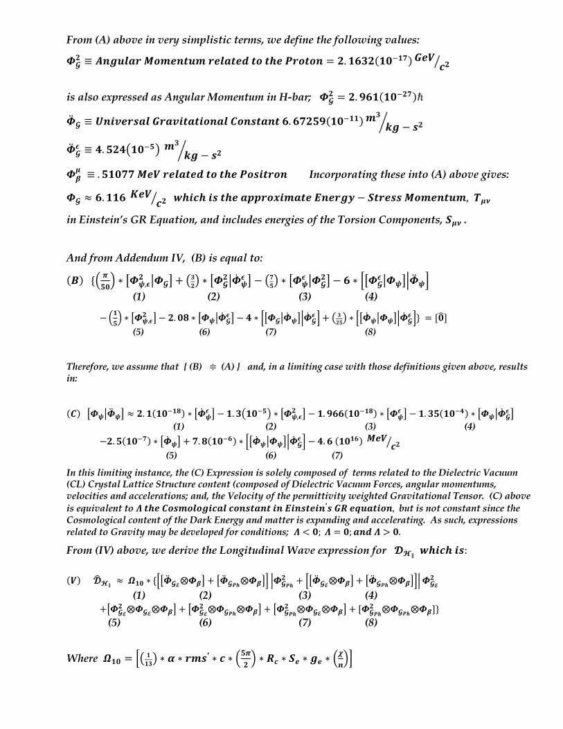
From (A) above in very simplistic terms, we define the following values:
𝜱𝓖𝟐 ≡ 𝑨𝒏𝒈𝒖𝒍𝒂𝒓𝑴𝒐𝒎𝒆𝒏𝒕𝒖𝒎𝒓𝒆𝒍𝒂𝒕𝒆𝒅𝒕𝒐𝒕𝒉𝒆𝑷𝒓𝒐𝒕𝒐𝒏 = 𝟐. 𝟏𝟔𝟑𝟐(𝟏𝟎1𝟏𝟕) 𝑮𝒆𝑽 𝒄𝟐�
is also expressed as Angular Momentum in H-bar; 𝜱𝓖𝟐 = 𝟐. 𝟗𝟔𝟏(𝟏𝟎1𝟐𝟕)ℏ
�̈�𝓖 ≡ 𝑼𝒏𝒊𝒗𝒆𝒓𝒔𝒂𝒍𝑮𝒓𝒂𝒗𝒊𝒕𝒂𝒕𝒊𝒐𝒏𝒂𝒍𝑪𝒐𝒏𝒔𝒕𝒂𝒏𝒕𝟔. 𝟔𝟕𝟐𝟓𝟗(𝟏𝟎1𝟏𝟏)𝒎𝟑
𝒌𝒈 − 𝒔𝟐f
�̈�𝓖𝝐 ≡ 𝟒. 𝟓𝟐𝟒j𝟏𝟎1𝟓k𝒎
𝟑
𝒌𝒈 − 𝒔𝟐f
𝜱𝜷𝝁 ≡. 𝟓𝟏𝟎𝟕𝟕𝑴𝒆𝑽𝒓𝒆𝒍𝒂𝒕𝒆𝒅𝒕𝒐𝒕𝒉𝒆𝑷𝒐𝒔𝒊𝒕𝒓𝒐𝒏 Incorporating these into (A) above gives:
𝜱𝓖 ≈ 𝟔. 𝟏𝟏𝟔𝑲𝒆𝑽 𝒄𝟐� 𝒘𝒉𝒊𝒄𝒉𝒊𝒔𝒕𝒉𝒆𝒂𝒑𝒑𝒓𝒐𝒙𝒊𝒎𝒂𝒕𝒆𝑬𝒏𝒆𝒓𝒈𝒚 − 𝑺𝒕𝒓𝒆𝒔𝒔𝑴𝒐𝒎𝒆𝒏𝒕𝒖𝒎, 𝑻𝝁𝝂
in Einstein’s GR Equation, and includes energies of the Torsion Components, 𝑺𝝁𝝂.
And from Addendum IV, (B) is equal to:
(𝑩){: 𝝅𝟓𝟎; ∗ =𝜱𝝍,𝝐
𝟐 @𝜱𝓖D + j𝟑𝟐k ∗ =𝜱𝓖𝟐@�̇�𝝍
𝝐 D − j𝟕𝟓k ∗ =𝜱𝝍𝝐 @𝜱𝓖
𝟐D − 𝟔 ∗ F=𝜱𝓖𝝐 @𝜱𝝍DG�̈�𝝍I
(1) (2) (3) (4)
−a𝟏𝟓b ∗ d𝜱𝝍,𝝐
𝟐 i − 𝟐. 𝟎𝟖 ∗ d𝜱𝝍g�̇�𝓖𝝐 i − 𝟒 ∗ jd𝜱𝓖g�̇�𝝍ik�̇�𝓖
𝝐 m + � 𝟑𝟐𝟓� ∗ jd�̇�𝝍g𝜱𝝍ik�̇�𝓖𝝐 m} = [𝟎U]
(5) (6) (7) (8)
Therefore, we assume that { (B) ≑ (A) } and, in a limiting case with those definitions given above, results in:
(𝑪)d𝜱𝝍g�̈�𝝍i ≈ 𝟐. 𝟏(𝟏𝟎:𝟏𝟖) ∗ d�̇�𝝍𝝐 i − 𝟏. 𝟑�𝟏𝟎:𝟓� ∗ d𝜱𝝍,𝝐
𝟐 i − 𝟏. 𝟗𝟔𝟔(𝟏𝟎:𝟏𝟖) ∗ d𝜱𝝍𝝐 i − 𝟏. 𝟑𝟓(𝟏𝟎:𝟒) ∗ d𝜱𝝍g�̇�𝓖
𝝐 i (1) (2) (3) (4) −𝟐. 𝟓(𝟏𝟎:𝟕) ∗ d�̇�𝝍i + 𝟕. 𝟖(𝟏𝟎:𝟔) ∗ jd�̇�𝝍g𝜱𝝍ik�̇�𝓖
𝝐 m − 𝟒. 𝟔(𝟏𝟎𝟏𝟔)𝑴𝒆𝑽 𝒄𝟐� (5) (6) (7)
In this limiting instance, the (C) Expression is solely composed of terms related to the Dielectric Vacuum (CL) Crystal Lattice Structure content (composed of Dielectric Vacuum Forces, angular momentums, velocities and accelerations; and, the Velocity of the permittivity weighted Gravitational Tensor. (C) above is equivalent to 𝜦𝒕𝒉𝒆𝑪𝒐𝒔𝒎𝒐𝒍𝒐𝒈𝒊𝒄𝒂𝒍𝒄𝒐𝒏𝒔𝒕𝒂𝒏𝒕𝒊𝒏𝑬𝒊𝒏𝒔𝒕𝒆𝒊𝒏′𝒔𝑮𝑹𝒆𝒒𝒖𝒂𝒕𝒊𝒐𝒏, but is not constant since the Cosmological content of the Dark Energy and matter is expanding and accelerating. As such, expressions related to Gravity may be developed for conditions; 𝜦 < 𝟎; 𝜦 = 𝟎; 𝒂𝒏𝒅𝜦 > 𝟎.
From (IV) above, we derive the Longitudinal Wave expression for 𝓓𝓗∥ 𝒘𝒉𝒊𝒄𝒉𝒊𝒔: (𝑽)𝓓U𝓗∥ ≈ 𝜴𝟏𝟎 ∗ {jd�̈�𝓖𝓔⨂𝜱𝜷i + d�̈�𝓖𝑷𝒉⨂𝜱𝜷im k𝜱𝓖𝑷𝒉
𝟐 + jd�̈�𝓖𝓔⨂𝜱𝜷i + d�̈�𝓖𝑷𝒉⨂𝜱𝜷imk𝜱𝓖𝓔𝟐
(1) (2) (3) (4) +d𝜱𝓖𝓔
𝟐 ⨂𝜱𝓖𝓔⨂𝜱𝜷i + d𝜱𝓖𝓔𝟐 ⨂𝜱𝓖𝑷𝒉⨂𝜱𝜷i + d𝜱𝓖𝑷𝒉
𝟐 ⨂𝜱𝓖𝓔⨂𝜱𝜷i + [𝜱𝓖𝑷𝒉𝟐 ⨂𝜱𝓖𝑷𝒉⨂𝜱𝜷]}
(5) (6) (7) (8) Where 𝜴𝟏𝟎 = Fj 𝟏𝟏𝟑k ∗ 𝜶 ∗ 𝒓𝒎𝒔
′ ∗ 𝒄 ∗ :𝟓𝝅𝟐; ∗ 𝑹𝒄 ∗ 𝑺𝒆 ∗ 𝒈𝒆 ∗ :
𝝌𝒏;I
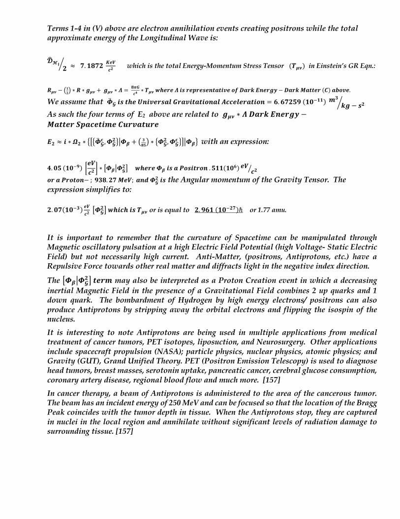
Terms 1-4 in (V) above are electron annihilation events creating positrons while the total approximate energy of the Longitudinal Wave is: 𝓓U𝓗∥
𝟐½ ≈ 𝟕. 𝟏𝟖𝟕𝟐 𝑲𝒆𝑽
𝒄𝟐 which is the total Energy-Momentum Stress Tensor (𝑻𝝁𝝂) in Einstein’s GR Eqn.:
𝑹𝝁𝝂 − S𝟏𝟐X ∗ 𝑹 ∗ 𝒈𝝁𝝂 +𝒈𝝁𝝂 ∗ 𝜦 =
𝟖𝝅𝑮𝒄𝟒∗ 𝑻𝝁𝝂𝒘𝒉𝒆𝒓𝒆𝜦𝒊𝒔𝒓𝒆𝒑𝒓𝒆𝒔𝒆𝒏𝒕𝒂𝒕𝒊𝒗𝒆𝒐𝒇𝑫𝒂𝒓𝒌𝑬𝒏𝒆𝒓𝒈𝒚 −𝑫𝒂𝒓𝒌𝑴𝒂𝒕𝒕𝒆𝒓(𝑪)𝒂𝒃𝒐𝒗𝒆.
We assume that �̈�𝓖𝒊𝒔𝒕𝒉𝒆𝑼𝒏𝒊𝒗𝒆𝒓𝒔𝒂𝒍𝑮𝒓𝒂𝒗𝒊𝒕𝒂𝒕𝒊𝒐𝒏𝒂𝒍𝑨𝒄𝒄𝒆𝒍𝒆𝒓𝒂𝒕𝒊𝒐𝒏 = 𝟔. 𝟔𝟕𝟐𝟓𝟗(𝟏𝟎:𝟏𝟏)𝒎𝟑
𝒌𝒈 − 𝒔𝟐½ As such the four terms of E2 above are related to 𝒈𝝁𝝂 ∗ 𝜦𝑫𝒂𝒓𝒌𝑬𝒏𝒆𝒓𝒈𝒚 −𝑴𝒂𝒕𝒕𝒆𝒓𝑺𝒑𝒂𝒄𝒆𝒕𝒊𝒎𝒆𝑪𝒖𝒓𝒗𝒂𝒕𝒖𝒓𝒆
𝑬𝟐 ≈ 𝒊 ∗ 𝜴𝟐 ∗ ede�̈�𝓖
𝝐 , 𝜱𝓖𝟐fg𝜱𝜷 + � 𝟑𝟖𝟓� ∗ e𝜱𝓖
𝟐 , 𝜱𝓖𝝐 fig𝜱𝜷f with an expression:
𝟒. 𝟎𝟓(𝟏𝟎E𝟗)�
𝒆𝑽𝒄𝟐 � ∗ M𝜱𝜷N𝜱𝓖
𝟐Q𝒘𝒉𝒆𝒓𝒆𝜱𝜷𝒊𝒔𝒂𝑷𝒐𝒔𝒊𝒕𝒓𝒐𝒏. 𝟓𝟏𝟏(𝟏𝟎𝟔) 𝒆𝑽 𝒄𝟐x
𝒐𝒓𝒂𝑷𝒓𝒐𝒕𝒐𝒏−; 𝟗𝟑𝟖. 𝟐𝟕𝑴𝒆𝑽; 𝒂𝒏𝒅𝜱𝓖𝟐 𝒊𝒔 the Angular momentum of the Gravity Tensor. The
expression simplifies to: 𝟐. 𝟎𝟕(𝟏𝟎:𝟑) 𝒆𝑽
𝒄𝟐d𝜱𝓖
𝟐i𝒘𝒉𝒊𝒄𝒉𝒊𝒔𝑻𝝁𝝂 or is equal to 𝟐. 𝟗𝟔𝟏(𝟏𝟎:𝟐𝟕)ℏ or 1.77 amu.
It is important to remember that the curvature of Spacetime can be manipulated through Magnetic oscillatory pulsation at a high Electric Field Potential (high Voltage- Static Electric Field) but not necessarily high current. Anti-Matter, (positrons, Antiprotons, etc.) have a Repulsive Force towards other real matter and diffracts light in the negative index direction.
The =𝜱𝜷@𝜱𝓖𝟐D𝒕𝒆𝒓𝒎 may also be interpreted as a Proton Creation event in which a decreasing
inertial Magnetic Field in the presence of a Gravitational Field combines 2 up quarks and 1 down quark. The bombardment of Hydrogen by high energy electrons/ positrons can also produce Antiprotons by stripping away the orbital electrons and flipping the isospin of the nucleus. It is interesting to note Antiprotons are being used in multiple applications from medical treatment of cancer tumors, PET isotopes, liposuction, and Neurosurgery. Other applications include spacecraft propulsion (NASA); particle physics, nuclear physics, atomic physics; and Gravity (GUT), Grand Unified Theory. PET (Positron Emission Telescopy) is used to diagnose head tumors, breast masses, serotonin uptake, pancreatic cancer, cerebral glucose consumption, coronary artery disease, regional blood flow and much more. [157] In cancer therapy, a beam of Antiprotons is administered to the area of the cancerous tumor. The beam has an incident energy of 250 MeV and can be focused so that the location of the Bragg Peak coincides with the tumor depth in tissue. When the Antiprotons stop, they are captured in nuclei in the local region and annihilate without significant levels of radiation damage to surrounding tissue. [157]

The expression for the transient component of the Longitudinal Wave (LW), (V) above is given by, 𝓓𝓗S�𝒊𝒔𝒆𝒒𝒖𝒊𝒗𝒂𝒍𝒆𝒏𝒕𝒕𝒐𝒕𝒉𝒆𝑷𝒐𝒚𝒏𝒕𝒊𝒏𝒈𝑽𝒆𝒄𝒕𝒐𝒓:
(𝑽. 𝟏)𝓓3𝓗= =𝜴𝒄 ∗ {[M�̈�𝓖N𝜱𝜷Q𝜱𝓖
𝟐]⨂[M�̈�𝓖N𝜱𝜷Q𝜱𝓖𝟐Q − ~M�̈�𝓖N𝜱𝜷Q𝜱𝓖
𝟐�⨂ ~M�̈�𝓖N𝜱𝓖𝟐Q𝜱𝜷� + [M�̈�𝓖N𝜱𝜷Q𝜱𝓖
𝟐]⨂[M𝜱𝓖𝟐N𝜱𝜷Q𝜱𝓖]
(1) (2) (3) −jd�̈�𝓖g𝜱𝜷i𝜱𝓖
𝟐m⨂ jd𝜱𝓖𝟐g𝜱𝓖i𝜱𝜷m − jd�̈�𝓖g𝜱𝓖
𝟐i𝜱𝜷m⨂ jd�̈�𝓖g𝜱𝜷i𝜱𝓖𝟐m
(4) (5) +jd�̈�𝓖g𝜱𝓖
𝟐i𝜱𝜷m⨂ jd�̈�𝓖g𝜱𝓖𝟐i𝜱𝜷m − jd�̈�𝓖g𝜱𝓖
𝟐i𝜱𝜷m⨂ jd𝜱𝓖𝟐g𝜱𝜷i𝜱𝓖m + [d�̈�𝓖|𝜱𝓖
𝟐i𝜱𝜷]⨂[d𝜱𝓖𝟐g𝜱𝓖i𝜱𝜷]}
(6) (7) (8)
Where 𝜴𝒄 =𝟏. 𝟒𝟖𝟗[𝑴𝒆𝑽 𝒄𝟐 −𝒎𝟐]⁄ Observe the Magnetic Field, Tensor is common to all eight terms which is an essential component needed for regauging. It is also significant that the Local Polarization of the Vacuum in proximity to a craft with a (HEEMFG) High Energy Electro-Magnetic Field Generator has the effect of Cohering the highly energetic and random quantum vacuum fields’ fluctuations which allows for a Quantum Vacuum envelope around the craft so it may move through any ambient field with an insignificant level of drag, (H. D. Froning). Such a device exists and has been built for the US Navy (various articles). The EM Field Generator consists of a shell of embedded poly-crystalline ferroelectric ceramic (including crystallized silicon graphite), an Electro-static Generator, (either a VandeGraf or Pellerton type), a thermal electric generator (Josephson junctions) which convert thermal energy into electric energy. A Pebble Bed fission reactor supplies the thermal energy. The electric motor spins the shell (axially rotating) at 30,000 to 50,000 RPM and this is simultaneously coupled with high vibrations (harmonic oscillatory pulsation) on the order of (𝟏𝟎𝟗 −𝟏𝟎𝟏𝟖)𝑯𝒛.
We can equate (V.1) above to the Energy Density equation: 𝑺𝑴𝒂𝒙 =𝒇𝑮𝟐 ∗ 𝜸 ∗ O𝝈𝟐
𝝐𝟎P ∗ [𝑹𝒓 ∗ 𝝎 + 𝑹𝝂 ∗ 𝝂 + 𝑽𝑹]
Note that there is the Permittivity term which is related to the Dielectric Vacuum Crystal Lattice content. In simplistic terms, the Poynting Vector Energy Density is: 𝑺𝑴𝒂𝒙 =
𝟏𝟐F𝝐𝟎 ∗ 𝑬"𝟐 +
𝟏𝝁𝟎∗ 𝑩"𝟐I
Where: 𝒇𝑮 ≡ 𝑮𝒆𝒐𝒎𝒆𝒕𝒓𝒊𝒄𝑺𝒉𝒂𝒑𝒆𝑭𝒂𝒄𝒕𝒐𝒓(𝑮𝒂𝒖𝒔𝒔 − 𝑩𝒐𝒏𝒆𝒕𝒕𝑪𝒉𝒂𝒓𝒂𝒄𝒕𝒆𝒓𝒊𝒔𝒕𝒊𝒄)𝒇𝒐𝒓𝒂𝒅𝒊𝒔𝒄 = 𝟏. 𝜸 ≡ 𝑹𝒆𝒍𝒂𝒕𝒊𝒗𝒊𝒔𝒕𝒊𝒄 𝑺′ 𝒕𝒓𝒆𝒕𝒄𝒉′𝒇𝒂𝒄𝒕𝒐𝒓[𝟏 √(𝟏 − 𝒗𝟐
𝒄𝟐� )
𝝈 ≡ 𝑺𝒖𝒓𝒇𝒂𝒄𝒆𝑪𝒉𝒂𝒓𝒈𝒆𝑫𝒆𝒏𝒔𝒊𝒕𝒚(𝒕𝒐𝒕𝒂𝒍𝒄𝒉𝒂𝒓𝒈𝒆𝒑𝒆𝒓𝒔𝒖𝒓𝒇𝒂𝒄𝒆𝒂𝒓𝒆𝒂) 𝝐𝟎 ≡ 𝑷𝒆𝒓𝒎𝒊𝒕𝒕𝒊𝒗𝒊𝒕𝒚𝒐𝒇𝒕𝒉𝒆𝑽𝒂𝒄𝒖𝒖𝒎𝑺𝒑𝒂𝒄𝒆 𝑬U ≡ 𝑬𝒍𝒆𝒄𝒕𝒓𝒊𝒄𝑭𝒊𝒆𝒍𝒅𝑻𝒆𝒏𝒔𝒐𝒓(𝑽𝒆𝒄𝒕𝒐𝒓) 𝑩U ≡ 𝑴𝒂𝒈𝒏𝒆𝒕𝒊𝒄𝑭𝒊𝒆𝒍𝒅𝑻𝒆𝒏𝒔𝒐𝒓(𝑽𝒆𝒄𝒕𝒐𝒓)
𝑹𝒓 ≡ 𝑹𝒂𝒅𝒊𝒖𝒔𝒐𝒇𝑹𝒐𝒕𝒂𝒕𝒊𝒐𝒏 (example given = 1 meter) 𝝎 ≡ 𝑨𝒏𝒈𝒖𝒍𝒂𝒓𝑭𝒓𝒆𝒒𝒖𝒆𝒏𝒄𝒚𝒐𝒇𝑽𝒊𝒃𝒓𝒂𝒕𝒊𝒐𝒏, 𝑹𝒂𝒅𝒔/𝒔𝒆𝒄 𝑹𝝂 ≡ 𝑯𝒂𝒓𝒎𝒐𝒏𝒊𝒄𝑶𝒔𝒄𝒊𝒍𝒍𝒂𝒕𝒊𝒐𝒏𝑨𝒎𝒑𝒍𝒊𝒕𝒖𝒅𝒆 𝝂 ≡ 𝑨𝒏𝒈𝒖𝒍𝒂𝒓𝑭𝒓𝒆𝒒𝒖𝒆𝒏𝒄𝒚𝒐𝒇𝒗𝒊𝒃𝒓𝒂𝒕𝒊𝒐𝒏, Hz 𝑽𝑹 ≡ 𝑪𝒖𝒓𝒗𝒊𝒍𝒊𝒏𝒆𝒂𝒓𝒕𝒓𝒂𝒏𝒔𝒍𝒂𝒕𝒊𝒐𝒏𝒔𝒑𝒆𝒆𝒅(𝒔𝒊𝒎𝒊𝒍𝒂𝒓𝒕𝒐𝒂𝑻𝒐𝒑) Acquired by attaching the propulsion unit to the system.
For the above example, with a 2-meter disc the system generates 𝟏𝟎𝟏𝟐 − 𝟏𝟎𝟏𝟔𝑻𝒆𝒓𝒓𝒂 −𝑾𝒂𝒕𝒕𝒔𝒑𝒆𝒓𝒎𝟐. which is an enormous amount of energy; enough to move an asteroid. The example given does not include the Quantum Vacuum Plasma (QVP) interactions which only amplify the effect.
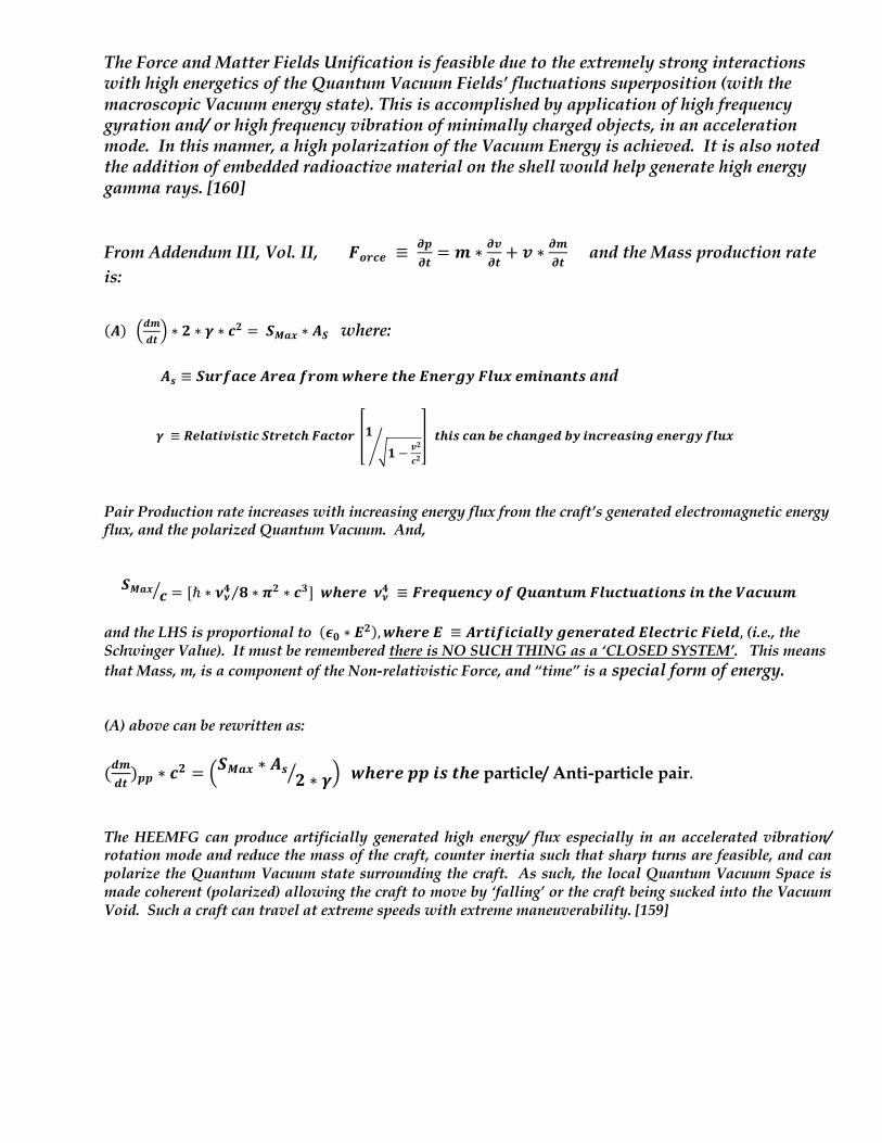
The Force and Matter Fields Unification is feasible due to the extremely strong interactions with high energetics of the Quantum Vacuum Fields’ fluctuations superposition (with the macroscopic Vacuum energy state). This is accomplished by application of high frequency gyration and/ or high frequency vibration of minimally charged objects, in an acceleration mode. In this manner, a high polarization of the Vacuum Energy is achieved. It is also noted the addition of embedded radioactive material on the shell would help generate high energy gamma rays. [160]
From Addendum III, Vol. II, 𝑭𝒐𝒓𝒄𝒆 ≡ 𝝏𝒑𝝏𝒕= 𝒎 ∗ 𝝏𝒗
𝝏𝒕+ 𝒗 ∗ 𝝏𝒎
𝝏𝒕 and the Mass production rate
is:
(𝑨)a𝒅𝒎𝒅𝒕b ∗ 𝟐 ∗ 𝜸 ∗ 𝒄𝟐 =𝑺𝑴𝒂𝒙 ∗ 𝑨𝑺 where:
𝑨𝒔 ≡ 𝑺𝒖𝒓𝒇𝒂𝒄𝒆𝑨𝒓𝒆𝒂𝒇𝒓𝒐𝒎𝒘𝒉𝒆𝒓𝒆𝒕𝒉𝒆𝑬𝒏𝒆𝒓𝒈𝒚𝑭𝒍𝒖𝒙𝒆𝒎𝒊𝒏𝒂𝒏𝒕𝒔and
𝜸 ≡ 𝑹𝒆𝒍𝒂𝒕𝒊𝒗𝒊𝒔𝒕𝒊𝒄𝑺𝒕𝒓𝒆𝒕𝒄𝒉𝑭𝒂𝒄𝒕𝒐𝒓 �𝟏�𝟏 − 𝒗𝟐
𝒄𝟐�
� 𝒕𝒉𝒊𝒔𝒄𝒂𝒏𝒃𝒆𝒄𝒉𝒂𝒏𝒈𝒆𝒅𝒃𝒚𝒊𝒏𝒄𝒓𝒆𝒂𝒔𝒊𝒏𝒈𝒆𝒏𝒆𝒓𝒈𝒚𝒇𝒍𝒖𝒙
Pair Production rate increases with increasing energy flux from the craft’s generated electromagnetic energy flux, and the polarized Quantum Vacuum. And,
𝑺𝑴𝒂𝒙 𝒄� = [ℏ ∗ 𝝂𝝂𝟒 𝟖 ∗ 𝝅𝟐 ∗ 𝒄𝟑]𝒘𝒉𝒆𝒓𝒆𝝂𝝂𝟒 ≡ 𝑭𝒓𝒆𝒒𝒖𝒆𝒏𝒄𝒚𝒐𝒇𝑸𝒖𝒂𝒏𝒕𝒖𝒎𝑭𝒍𝒖𝒄𝒕𝒖𝒂𝒕𝒊𝒐𝒏𝒔𝒊𝒏𝒕𝒉𝒆𝑽𝒂𝒄𝒖𝒖𝒎⁄ and the LHS is proportional to (𝝐𝟎 ∗ 𝑬𝟐),𝒘𝒉𝒆𝒓𝒆𝑬 ≡ 𝑨𝒓𝒕𝒊𝒇𝒊𝒄𝒊𝒂𝒍𝒍𝒚𝒈𝒆𝒏𝒆𝒓𝒂𝒕𝒆𝒅𝑬𝒍𝒆𝒄𝒕𝒓𝒊𝒄𝑭𝒊𝒆𝒍𝒅, (i.e., the Schwinger Value). It must be remembered there is NO SUCH THING as a ‘CLOSED SYSTEM’. This means that Mass, m, is a component of the Non-relativistic Force, and “time” is a special form of energy.
(A) above can be rewritten as: (𝒅𝒎𝒅𝒕)𝒑𝒑 ∗ 𝒄𝟐 = :𝑺𝑴𝒂𝒙 ∗ 𝑨𝒔 𝟐 ∗ 𝜸� ; 𝒘𝒉𝒆𝒓𝒆𝒑𝒑𝒊𝒔𝒕𝒉𝒆particle/ Anti-particle pair.
The HEEMFG can produce artificially generated high energy/ flux especially in an accelerated vibration/ rotation mode and reduce the mass of the craft, counter inertia such that sharp turns are feasible, and can polarize the Quantum Vacuum state surrounding the craft. As such, the local Quantum Vacuum Space is made coherent (polarized) allowing the craft to move by ‘falling’ or the craft being sucked into the Vacuum Void. Such a craft can travel at extreme speeds with extreme maneuverability. [159]
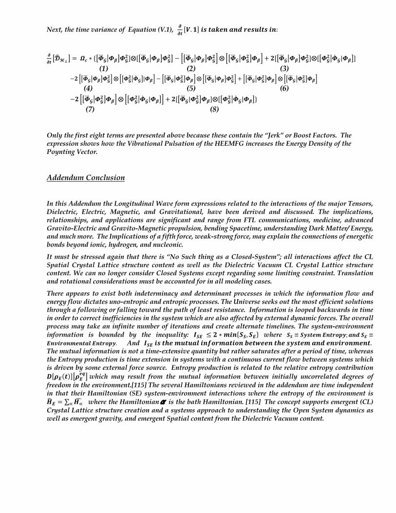
Next, the time variance of Equation (V.1), 𝝏𝝏𝒕[𝑽. 𝟏]𝒊𝒔𝒕𝒂𝒌𝒆𝒏𝒂𝒏𝒅𝒓𝒆𝒔𝒖𝒍𝒕𝒔𝒊𝒏:
𝝏𝝏𝒕M𝓓3𝓗=Q = 𝜴𝒄 ∗ {M𝜱z𝓖N𝜱𝜷Q𝜱𝓖
𝟐]⨂[M𝜱z𝓖N𝜱𝜷Q𝜱𝓖𝟐Q − ~M𝜱z𝓖N𝜱𝜷Q𝜱𝓖
𝟐�⨂ ~M𝜱z𝓖N𝜱𝓖𝟐Q𝜱𝜷� + 𝟐[M𝜱z𝓖N𝜱𝜷Q𝜱𝓖
𝟐]⨂[M𝜱𝓖𝟐N�̇�𝓖|𝜱𝜷Q]
(1) (2) (3) −𝟐 Re𝜱�𝓖W𝜱𝜷f𝜱𝓖
𝟐[⨂ Re𝜱𝓖𝟐W�̇�𝓖f|𝜱𝜷[ − Re𝜱�𝓖W𝜱𝓖
𝟐f𝜱𝜷[⨂Re𝜱�𝓖W𝜱𝜷f𝜱𝓖𝟐[ + Re𝜱�𝓖W𝜱𝓖
𝟐f𝜱𝜷[⨂ Re𝜱�𝓖W𝜱𝓖𝟐f𝜱𝜷[
(4) (5) (6) −𝟐 ~M𝜱z𝓖N𝜱𝓖
𝟐Q𝜱𝜷�⨂ ~M𝜱𝓖𝟐N�̇�𝓖|𝜱𝜷Q� + 𝟐[M𝜱z𝓖|𝜱𝓖
𝟐Q𝜱𝜷]⨂[M𝜱𝓖𝟐N�̇�𝓖|𝜱𝜷Q}
(7) (8) Only the first eight terms are presented above because these contain the “Jerk” or Boost Factors. The expression shows how the Vibrational Pulsation of the HEEMFG increases the Energy Density of the Poynting Vector.
Addendum Conclusion In this Addendum the Longitudinal Wave form expressions related to the interactions of the major Tensors, Dielectric, Electric, Magnetic, and Gravitational, have been derived and discussed. The implications, relationships, and applications are significant and range from FTL communications, medicine, advanced Gravito-Electric and Gravito-Magnetic propulsion, bending Spacetime, understanding Dark Matter/ Energy, and much more. The Implications of a fifth force, weak-strong force, may explain the connections of energetic bonds beyond ionic, hydrogen, and nucleonic.
It must be stressed again that there is “No Such thing as a Closed-System”; all interactions affect the CL Spatial Crystal Lattice structure content as well as the Dielectric Vacuum CL Crystal Lattice structure content. We can no longer consider Closed Systems except regarding some limiting constraint. Translation and rotational considerations must be accounted for in all modeling cases.
There appears to exist both indeterminacy and determinant processes in which the information flow and energy flow dictates uno-entropic and entropic processes. The Universe seeks out the most efficient solutions through a following or falling toward the path of least resistance. Information is looped backwards in time in order to correct inefficiencies in the system which are also affected by external dynamic forces. The overall process may take an infinite number of iterations and create alternate timelines. The system-environment information is bounded by the inequality: 𝑰𝑺𝑬 ≤ 𝟐 ∗ 𝒎𝒊𝒏{𝑺𝑺, 𝑺𝑬} where 𝑺𝑺 ≡ 𝑺𝒚𝒔𝒕𝒆𝒎𝑬𝒏𝒕𝒓𝒐𝒑𝒚; 𝒂𝒏𝒅𝑺𝑬 ≡𝑬𝒏𝒗𝒊𝒓𝒐𝒏𝒎𝒆𝒏𝒕𝒂𝒍𝑬𝒏𝒕𝒓𝒐𝒑𝒚. And 𝑰𝑺𝑬𝒊𝒔𝒕𝒉𝒆𝒎𝒖𝒕𝒖𝒂𝒍𝒊𝒏𝒇𝒐𝒓𝒎𝒂𝒕𝒊𝒐𝒏𝒃𝒆𝒕𝒘𝒆𝒆𝒏𝒕𝒉𝒆𝒔𝒚𝒔𝒕𝒆𝒎𝒂𝒏𝒅𝒆𝒏𝒗𝒊𝒓𝒐𝒏𝒎𝒆𝒏𝒕. The mutual information is not a time-extensive quantity but rather saturates after a period of time, whereas the Entropy production is time extension in systems with a continuous current flow between systems which is driven by some external force source. Entropy production is related to the relative entropy contribution 𝑫[𝝆𝑬(𝒕)]d𝝆𝑬
𝒆𝒒iwhich may result from the mutual information between initially uncorrelated degrees of freedom in the environment.[115] The several Hamiltonians reviewed in the addendum are time independent in that their Hamiltonian (SE) system-environment interactions where the entropy of the environment is 𝑯U𝑬 = ∑ 𝑯∝Q∝ where the Hamiltonianα is the bath Hamiltonian. [115] The concept supports emergent (CL) Crystal Lattice structure creation and a systems approach to understanding the Open System dynamics as well as emergent gravity, and emergent Spatial content from the Dielectric Vacuum content.
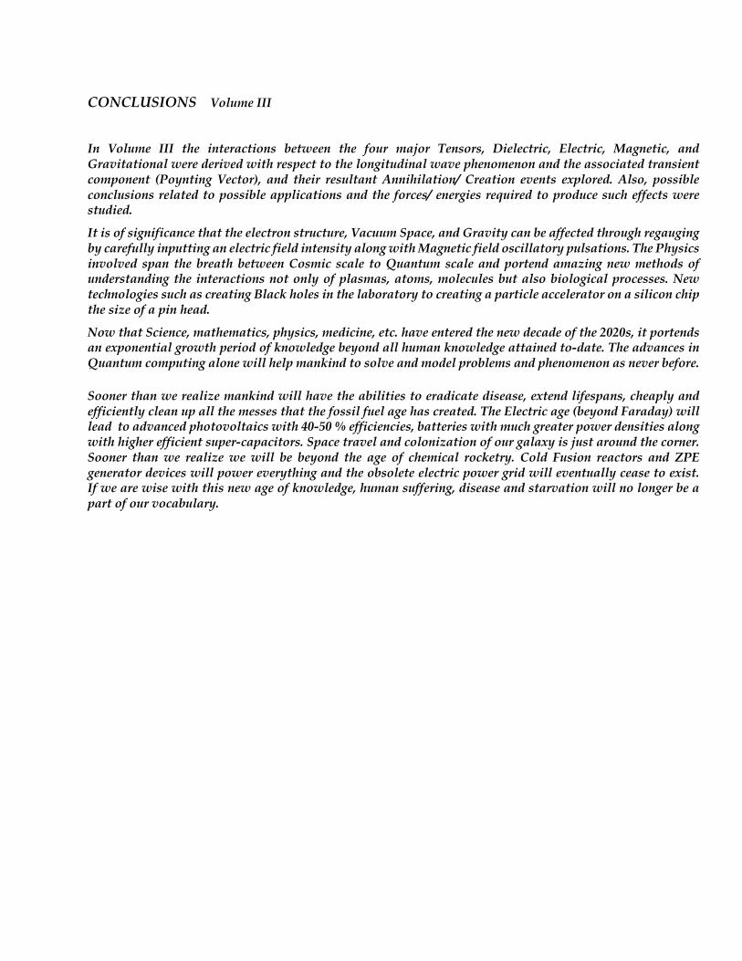
CONCLUSIONS Volume III
In Volume III the interactions between the four major Tensors, Dielectric, Electric, Magnetic, and Gravitational were derived with respect to the longitudinal wave phenomenon and the associated transient component (Poynting Vector), and their resultant Annihilation/ Creation events explored. Also, possible conclusions related to possible applications and the forces/ energies required to produce such effects were studied.
It is of significance that the electron structure, Vacuum Space, and Gravity can be affected through regauging by carefully inputting an electric field intensity along with Magnetic field oscillatory pulsations. The Physics involved span the breath between Cosmic scale to Quantum scale and portend amazing new methods of understanding the interactions not only of plasmas, atoms, molecules but also biological processes. New technologies such as creating Black holes in the laboratory to creating a particle accelerator on a silicon chip the size of a pin head.
Now that Science, mathematics, physics, medicine, etc. have entered the new decade of the 2020s, it portends an exponential growth period of knowledge beyond all human knowledge attained to-date. The advances in Quantum computing alone will help mankind to solve and model problems and phenomenon as never before. Sooner than we realize mankind will have the abilities to eradicate disease, extend lifespans, cheaply and efficiently clean up all the messes that the fossil fuel age has created. The Electric age (beyond Faraday) will lead to advanced photovoltaics with 40-50 % efficiencies, batteries with much greater power densities along with higher efficient super-capacitors. Space travel and colonization of our galaxy is just around the corner. Sooner than we realize we will be beyond the age of chemical rocketry. Cold Fusion reactors and ZPE generator devices will power everything and the obsolete electric power grid will eventually cease to exist. If we are wise with this new age of knowledge, human suffering, disease and starvation will no longer be a part of our vocabulary.
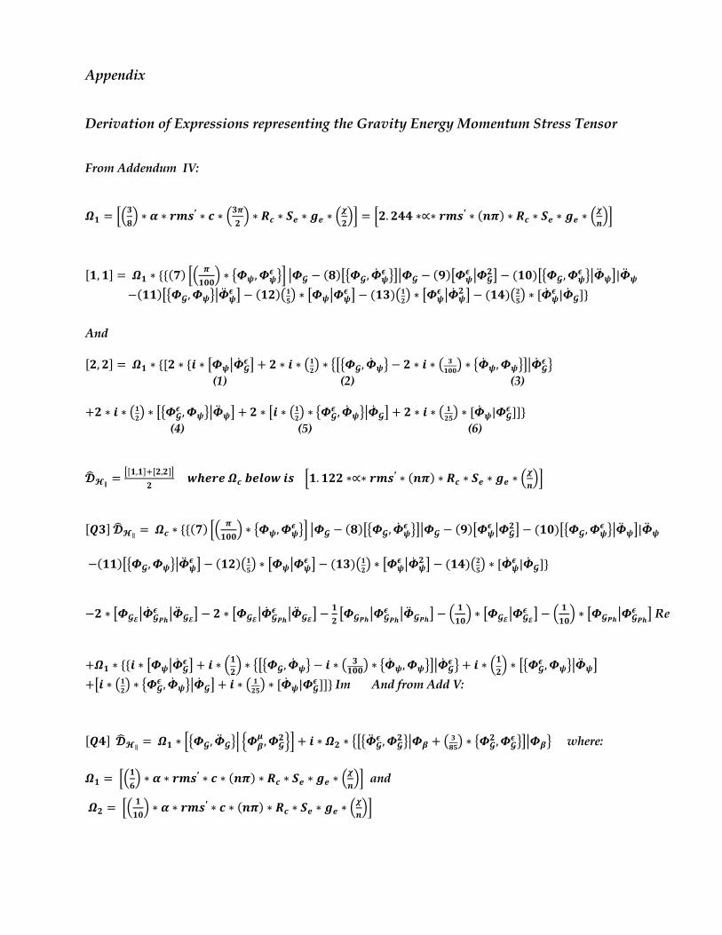
Appendix
Derivation of Expressions representing the Gravity Energy Momentum Stress Tensor
From Addendum IV:
𝜴𝟏 = ja𝟑𝟖b ∗ 𝜶 ∗ 𝒓𝒎𝒔′ ∗ 𝒄 ∗ a𝟑𝝅
𝟐b ∗ 𝑹𝒄 ∗ 𝑺𝒆 ∗ 𝒈𝒆 ∗ a
𝝌𝟐bm = j𝟐. 𝟐𝟒𝟒 ∗∝∗ 𝒓𝒎𝒔′ ∗ (𝒏𝝅) ∗ 𝑹𝒄 ∗ 𝑺𝒆 ∗ 𝒈𝒆 ∗ a
𝝌𝒏bm
[𝟏, 𝟏] = 𝜴𝟏 ∗ {{(𝟕) ja
𝝅𝟏𝟎𝟎b ∗ e𝜱𝝍, 𝜱𝝍
𝝐 fm g𝜱𝓖 − (𝟖)de𝜱𝓖, �̇�𝝍𝝐 fig𝜱𝓖 − (𝟗)d𝜱𝝍
𝝐 g𝜱𝓖𝟐i − (𝟏𝟎)de𝜱𝓖, 𝜱𝝍
𝝐 fg�̈�𝝍i|�̈�𝝍 −(𝟏𝟏)de𝜱𝓖, 𝜱𝝍fg�̈�𝝍
𝝐 i − (𝟏𝟐)�𝟏𝟓� ∗ d𝜱𝝍g𝜱𝝍𝝐 i − (𝟏𝟑)�𝟏𝟐� ∗ d𝜱𝝍
𝝐 g�̇�𝝍𝟐 i − (𝟏𝟒)�𝟐𝟓� ∗ [�̇�𝝍
𝝐 |�̇�𝓖]}
And [𝟐, 𝟐] = 𝜴𝟏 ∗ {[𝟐 ∗ {𝒊 ∗ d𝜱𝝍g�̇�𝓖
𝝐 i + 𝟐 ∗ 𝒊 ∗ �𝟏𝟐� ∗ ede𝜱𝓖, �̇�𝝍f − 𝟐 ∗ 𝒊 ∗ � 𝟑𝟏𝟎𝟎� ∗ e�̇�𝝍, 𝜱𝝍fig�̇�𝓖
𝝐 f (1) (2) (3) +𝟐 ∗ 𝒊 ∗ �𝟏𝟐� ∗ de𝜱𝓖
𝝐 , 𝜱𝝍fg�̈�𝝍i + 𝟐 ∗ d𝒊 ∗ �𝟏𝟐� ∗ e𝜱𝓖𝝐 , �̇�𝝍fg�̇�𝓖i + 𝟐 ∗ 𝒊 ∗ � 𝟏𝟐𝟓� ∗ [�̇�𝝍|𝜱𝓖
𝝐 ]]} (4) (5) (6)
𝓓U𝓗∥ =j[𝟏,𝟏]T[𝟐,𝟐]m
𝟐𝒘𝒉𝒆𝒓𝒆𝜴𝒄𝒃𝒆𝒍𝒐𝒘𝒊𝒔 j𝟏. 𝟏𝟐𝟐 ∗∝∗ 𝒓𝒎𝒔′ ∗ (𝒏𝝅) ∗ 𝑹𝒄 ∗ 𝑺𝒆 ∗ 𝒈𝒆 ∗ a
𝝌𝒏bm
[𝑸𝟑]𝓓U𝓗∥ =𝜴𝒄 ∗ {{(𝟕) ja𝝅𝟏𝟎𝟎b ∗ e𝜱𝝍, 𝜱𝝍
𝝐 fm g𝜱𝓖 − (𝟖)de𝜱𝓖, �̇�𝝍𝝐 fig𝜱𝓖 − (𝟗)d𝜱𝝍
𝝐 g𝜱𝓖𝟐i − (𝟏𝟎)de𝜱𝓖, 𝜱𝝍
𝝐 fg�̈�𝝍i|�̈�𝝍 −(𝟏𝟏)de𝜱𝓖, 𝜱𝝍fg�̈�𝝍
𝝐 i − (𝟏𝟐)�𝟏𝟓� ∗ d𝜱𝝍g𝜱𝝍𝝐 i − (𝟏𝟑)�𝟏𝟐� ∗ d𝜱𝝍
𝝐 g�̇�𝝍𝟐 i − (𝟏𝟒)�𝟐𝟓� ∗ [�̇�𝝍
𝝐 |�̇�𝓖]}
−𝟐 ∗ d𝜱𝓖𝓔g�̇�𝓖𝑷𝒉𝝐 g�̈�𝓖𝓔i − 𝟐 ∗ d𝜱𝓖𝓔g�̇�𝓖𝑷𝒉
𝝐 g�̈�𝓖𝓔i −𝟏𝟐d𝜱𝓖𝑷𝒉g𝜱𝓖𝑷𝒉
𝝐 g�̈�𝓖𝑷𝒉i − a𝟏𝟏𝟎b ∗ d𝜱𝓖𝓔g𝜱𝓖𝓔
𝝐 i − a 𝟏𝟏𝟎b ∗ d𝜱𝓖𝑷𝒉g𝜱𝓖𝑷𝒉
𝝐 i Re
+𝜴𝟏 ∗ {{𝒊 ∗ d𝜱𝝍g�̇�𝓖𝝐 i + 𝒊 ∗ a𝟏
𝟐b ∗ ede𝜱𝓖, �̇�𝝍f − 𝒊 ∗ � 𝟑
𝟏𝟎𝟎� ∗ e�̇�𝝍, 𝜱𝝍fig�̇�𝓖𝝐 f + 𝒊 ∗ a𝟏
𝟐b ∗ de𝜱𝓖
𝝐 , 𝜱𝝍fg�̈�𝝍i +d𝒊 ∗ �𝟏𝟐� ∗ e𝜱𝓖
𝝐 , �̇�𝝍fg�̇�𝓖i + 𝒊 ∗ � 𝟏𝟐𝟓� ∗ [�̇�𝝍|𝜱𝓖𝝐 ]]}Im And from Add V:
[𝑸𝟒]𝓓U𝓗∥ =𝜴𝟏 ∗ je𝜱𝓖, �̈�𝓖fk c𝜱𝜷𝝁 , 𝜱𝓖
𝟐lm + 𝒊 ∗ 𝜴𝟐 ∗ ede�̈�𝓖𝝐 , 𝜱𝓖
𝟐fg𝜱𝜷 + � 𝟑𝟖𝟓� ∗ e𝜱𝓖𝟐 , 𝜱𝓖
𝝐 fig𝜱𝜷f where: 𝜴𝟏 = ja
𝟏𝟔b ∗ 𝜶 ∗ 𝒓𝒎𝒔′ ∗ 𝒄 ∗ (𝒏𝝅) ∗ 𝑹𝒄 ∗ 𝑺𝒆 ∗ 𝒈𝒆 ∗ a
𝝌𝒏bm and
𝜴𝟐 = ja𝟏𝟏𝟎b ∗ 𝜶 ∗ 𝒓𝒎𝒔′ ∗ 𝒄 ∗ (𝒏𝝅) ∗ 𝑹𝒄 ∗ 𝑺𝒆 ∗ 𝒈𝒆 ∗ a
𝝌𝒏bm
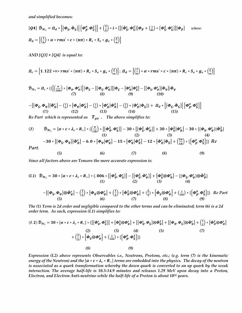
and simplified becomes: [𝑸𝟒]𝓓U𝓗∥ = 𝜴𝒅 ∗ je𝜱𝓖, �̈�𝓖fk c𝜱𝜷
𝝁 , 𝜱𝓖𝟐lm + a𝟑
𝟓b ∗ 𝒊 ∗ ede�̈�𝓖
𝝐 , 𝜱𝓖𝟐fg𝜱𝜷 + � 𝟑𝟖𝟓� ∗ e𝜱𝓖
𝟐 , 𝜱𝓖𝝐 fig𝜱𝜷f where:
𝜴𝒅 = ja𝟏
𝟔b ∗ 𝜶 ∗ 𝒓𝒎𝒔′ ∗ 𝒄 ∗ (𝒏𝝅) ∗ 𝑹𝒄 ∗ 𝑺𝒆 ∗ 𝒈𝒆 ∗ a
𝝌𝒏bm
AND [Q3] + [Q4] is equal to:
𝜴𝒄 = j𝟏. 𝟏𝟐𝟐 ∗∝∗ 𝒓𝒎𝒔′ ∗ (𝒏𝝅) ∗ 𝑹𝒄 ∗ 𝑺𝒆 ∗ 𝒈𝒆 ∗ a𝝌𝒏bm ;𝜴𝒅 = ja𝟏
𝟔b ∗ 𝜶 ∗ 𝒓𝒎𝒔′ ∗ 𝒄 ∗ (𝒏𝝅) ∗ 𝑹𝒄 ∗ 𝑺𝒆 ∗ 𝒈𝒆 ∗ a
𝝌𝒏bm
𝓓3𝓗∥ = 𝜴𝒄 ∗ {{~J𝝅𝟏𝟎𝟎K ∗ O𝜱𝝍, 𝜱𝝍
𝝐 P� N𝜱𝓖 − MO𝜱𝓖, �̇�𝝍𝝐 PQN𝜱𝓖 − M𝜱𝝍
𝝐 N𝜱𝓖𝟐Q − MO𝜱𝓖, 𝜱𝝍
𝝐 PN�̈�𝝍Q|�̈�𝝍 (7) (8) (9) (10) −de𝜱𝓖, 𝜱𝝍fg�̈�𝝍
𝝐 i − �𝟏𝟓� ∗ d𝜱𝝍g𝜱𝝍𝝐 i − �𝟏𝟐� ∗ d𝜱𝝍
𝝐 g�̇�𝝍𝟐 i − �𝟐𝟓� ∗ [�̇�𝝍
𝝐 |�̇�𝓖]} + 𝜴𝒅 ∗ je𝜱𝓖, �̈�𝓖fk c𝜱𝜷𝝁 , 𝜱𝓖
𝟐lm (!!) (12) (13) (14) (15) Re Part which is represented as 𝑻𝝁𝝂 . The above simplifies to: (𝑰)𝓓U𝓗∥ = [𝜶 ∗ 𝒄 ∗ 𝝀𝒄 ∗ 𝑹∞] ∗ {a
𝝅𝟏𝟖b ∗ de𝜱𝝍
𝟐 , 𝜱𝓖𝝐 fi − 𝟑𝟎 ∗ de𝜱𝓖
𝟐 , �̇�𝝍𝝐 fi + 𝟑𝟎 ∗ d𝜱𝓖
𝟐g𝜱𝝍𝝐 i − 𝟑𝟎 ∗ [{𝜱𝓖, 𝜱𝝍
𝝐 }|�̈�𝝍𝟐 ]
(1) (2) (3) (4) −𝟑𝟎 ∗ de𝜱𝓖, 𝜱𝝍fg�̈�𝝍
𝝐 i − 𝟔. 𝟎 ∗ d𝜱𝝍g𝜱𝝍𝝐 i − 𝟏𝟓 ∗ d𝜱𝝍
𝝐 g�̇�𝝍𝟐 i − 𝟏𝟐 ∗ d�̇�𝝍
𝝐 g�̇�𝓖i + a𝟓𝝅𝟏𝟖b ∗ [c𝜱𝜷
𝝁 , 𝜱𝓖𝟑l]} Re
Part. (5) (6) (7) (8) (9)
Since all factors above are Tensors the more accurate expression is:
(I.1) 𝓓U𝓗∥ = 𝟑𝟎 ∗ [𝜶 ∗ 𝒄 ∗ 𝝀𝒄 ∗ 𝑹∞] ∗ {. 𝟎𝟎𝟔 ∗ de𝜱𝝍𝟐 , 𝜱𝓖
𝝐 fi − de𝜱𝓖𝟐 , �̇�𝝍
𝝐 fi + d𝜱𝓖𝟐⨂𝜱𝝍
𝝐 i − [{𝜱𝓖, 𝜱𝝍𝝐 }⨂�̈�𝝍
𝟐 ] (1) (2) (3) (4) −de𝜱𝓖, 𝜱𝝍f⨂�̈�𝝍
𝝐 i − a𝟏𝟓b ∗ d𝜱𝝍⨂𝜱𝝍
𝝐 i + a𝟏𝟐b ∗ d�̇�𝝍
𝟐⨂𝜱𝝍𝝐 i + (𝟐
𝟓) ∗ j�̇�𝓖⨂𝜱̇ 𝝍
𝝐 m + � 𝟑𝟏𝟎𝟎� ∗ [c𝜱𝜷
𝝁 , 𝜱𝓖𝟑l]} Re Part
(5) (6) (7) (8) (9)
The (1) Term is 2d order and negligible compared to the other terms and can be eliminated; term (6) is a 2d order term. As such, expression (I.1) simplifies to: (𝑰. 𝟐)𝓓3𝓗∥ = 𝟑𝟎 ∗ [𝜶 ∗ 𝒄 ∗ 𝝀𝒄 ∗ 𝑹∞] ∗ {MO�̇�𝝍
𝝐 , 𝜱𝓖𝟐PQ + M𝜱𝓖
𝟐⨂𝜱𝝍𝝐 Q + MO𝜱𝝍
𝝐 , 𝜱𝓖P⨂�̈�𝝍𝟐 Q + MO𝜱𝝍, 𝜱𝓖P⨂�̈�𝝍
𝝐 Q + J𝟏𝟐K ∗ M�̇�𝝍𝟐⨂𝜱𝝍
𝝐 Q
(2) (3) (4) (5) (7) +a𝟐
𝟓b ∗ j�̇�𝓖⨂𝜱̇ 𝝍
𝝐 m + � 𝟑𝟏𝟎𝟎� ∗ [c𝜱𝜷
𝝁 , 𝜱𝓖𝟑l]}
(8) (9)
Expression (I.2) above represents Observables i.e., Neutrons, Protons, etc.; (e.g. term (7) is the kinematic energy of the Neutron) and the [𝜶 ∗ 𝒄 ∗ 𝝀𝒄 ∗ 𝑹∞] terms are embedded into the physics. The decay of the neutron is associated as a quark transformation whereby the down quark is converted to an up quark by the weak interaction. The average half-life is 10.3-14.9 minutes and releases 1.29 MeV upon decay into a Proton, Electron, and Electron Anti-neutrino while the half-life of a Proton is about 1032 years.
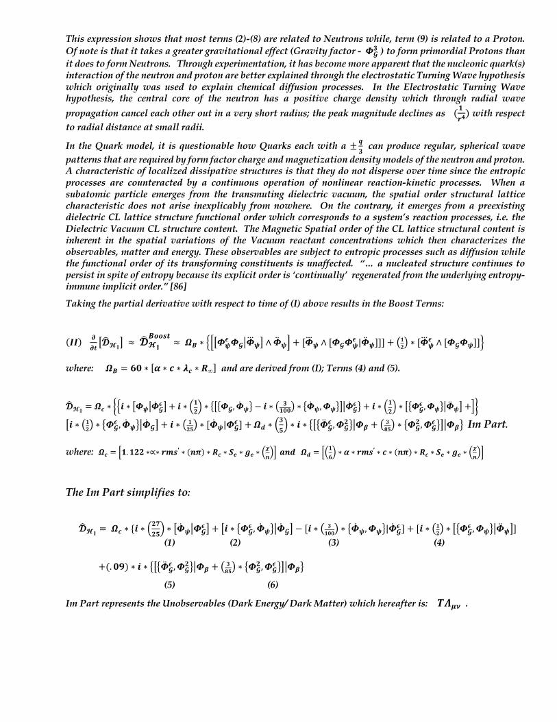
This expression shows that most terms (2)-(8) are related to Neutrons while, term (9) is related to a Proton. Of note is that it takes a greater gravitational effect (Gravity factor -𝜱𝓖
𝟑 ) to form primordial Protons than it does to form Neutrons. Through experimentation, it has become more apparent that the nucleonic quark(s) interaction of the neutron and proton are better explained through the electrostatic Turning Wave hypothesis which originally was used to explain chemical diffusion processes. In the Electrostatic Turning Wave hypothesis, the central core of the neutron has a positive charge density which through radial wave propagation cancel each other out in a very short radius; the peak magnitude declines as (𝟏
𝒓𝟒) with respect
to radial distance at small radii.
In the Quark model, it is questionable how Quarks each with a ± 𝒒𝟑 can produce regular, spherical wave
patterns that are required by form factor charge and magnetization density models of the neutron and proton. A characteristic of localized dissipative structures is that they do not disperse over time since the entropic processes are counteracted by a continuous operation of nonlinear reaction-kinetic processes. When a subatomic particle emerges from the transmuting dielectric vacuum, the spatial order structural lattice characteristic does not arise inexplicably from nowhere. On the contrary, it emerges from a preexisting dielectric CL lattice structure functional order which corresponds to a system’s reaction processes, i.e. the Dielectric Vacuum CL structure content. The Magnetic Spatial order of the CL lattice structural content is inherent in the spatial variations of the Vacuum reactant concentrations which then characterizes the observables, matter and energy. These observables are subject to entropic processes such as diffusion while the functional order of its transforming constituents is unaffected. “… a nucleated structure continues to persist in spite of entropy because its explicit order is ‘continually’ regenerated from the underlying entropy-immune implicit order.” [86]
Taking the partial derivative with respect to time of (I) above results in the Boost Terms:
(𝑰𝑰) 𝝏𝝏𝒕d𝓓U𝓗∥i ≈ 𝓓U𝓗∥
𝑩𝒐𝒐𝒔𝒕≈𝜴𝑩 ∗ cjd𝜱𝝍
𝝐𝜱𝓖g𝜱�𝝍i ∧ �̈�𝝍m + [𝜱�𝝍 ∧ [𝜱𝓖𝜱𝝍𝝐 |�̈�𝝍]]] + �𝟏𝟐� ∗ [𝜱�𝝍
𝝐 ∧ [𝜱𝓖𝜱𝝍]]l where: 𝜴𝑩 = 𝟔𝟎 ∗ [𝜶 ∗ 𝒄 ∗ 𝝀𝒄 ∗ 𝑹∞] and are derived from (I); Terms (4) and (5).
𝓓3𝓗∥ = 𝜴𝒄 ∗ �L𝒊 ∗ M𝜱𝝍N�̇�𝓖𝝐 Q + 𝒊 ∗ J𝟏𝟐K ∗ OMO𝜱𝓖, �̇�𝝍P − 𝒊 ∗ k 𝟑
𝟏𝟎𝟎l ∗ O�̇�𝝍, 𝜱𝝍PQN�̇�𝓖𝝐 P + 𝒊 ∗ J𝟏𝟐K ∗ MO𝜱𝓖
𝝐 , 𝜱𝝍PN�̈�𝝍Q +��
d𝒊 ∗ �𝟏𝟐� ∗ e𝜱𝓖𝝐 , �̇�𝝍fg�̇�𝓖i + 𝒊 ∗ � 𝟏𝟐𝟓� ∗ [�̇�𝝍|𝜱𝓖
𝝐 ] + 𝜴𝒅 ∗ a𝟑𝟓b ∗ 𝒊 ∗ ede�̈�𝓖
𝝐 , 𝜱𝓖𝟐fg𝜱𝜷 + � 𝟑𝟖𝟓� ∗ e𝜱𝓖
𝟐 , 𝜱𝓖𝝐 fig𝜱𝜷f Im Part.
where: 𝜴𝒄 = R𝟏. 𝟏𝟐𝟐 ∗∝∗ 𝒓𝒎𝒔′ ∗ (𝒏𝝅) ∗ 𝑹𝒄 ∗ 𝑺𝒆 ∗ 𝒈𝒆 ∗ O
𝝌𝒏P[ 𝒂𝒏𝒅𝜴𝒅 = RO𝟏𝟔P ∗ 𝜶 ∗ 𝒓𝒎𝒔
′ ∗ 𝒄 ∗ (𝒏𝝅) ∗ 𝑹𝒄 ∗ 𝑺𝒆 ∗ 𝒈𝒆 ∗ O𝝌𝒏P[
The Im Part simplifies to:
𝓓U𝓗∥ =𝜴𝒄 ∗ {𝒊 ∗ a𝟐𝟕𝟐𝟓b ∗ d�̇�𝝍g𝜱𝓖
𝝐 i + d𝒊 ∗ e𝜱𝓖𝝐 , �̇�𝝍fg�̇�𝓖i − [𝒊 ∗ � 𝟑
𝟏𝟎𝟎� ∗ e�̇�𝝍, 𝜱𝝍f|�̇�𝓖𝝐 ] + [𝒊 ∗ �𝟏𝟐� ∗ de𝜱𝓖
𝝐 , 𝜱𝝍fg�̈�𝝍i] (1) (2) (3) (4) +(. 𝟎𝟗) ∗ 𝒊 ∗ ede�̈�𝓖
𝝐 , 𝜱𝓖𝟐fg𝜱𝜷 + � 𝟑𝟖𝟓� ∗ e𝜱𝓖
𝟐 , 𝜱𝓖𝝐 fig𝜱𝜷f
(5) (6)
Im Part represents the Unobservables (Dark Energy/ Dark Matter) which hereafter is: 𝑻𝜦𝝁𝝂 .
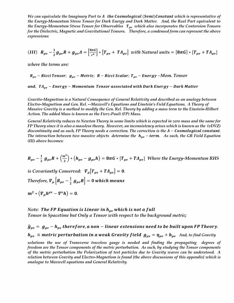
We can equivalate the Imaginary Part to 𝜦𝒕𝒉𝒆𝑪𝒐𝒔𝒎𝒐𝒍𝒐𝒈𝒊𝒄𝒂𝒍(𝑺𝒆𝒎𝒊)𝑪𝒐𝒏𝒔𝒕𝒂𝒏𝒕 which is representative of the Energy-Momentum Stress Tensor for Dark Energy and Dark Matter. And, the Real Part equivalent to the Energy-Momentum Stress Tensor for Observables 𝑻𝝁𝝂 which also incorporates the Contorsion Tensors for the Dielectric, Magnetic and Gravitational Tensors. Therefore, a condensed form can represent the above expressions:
(𝑰𝑰𝑰)𝑹𝝁𝝂 −𝟏𝟐𝒈𝝁𝝂𝑹 + 𝒈𝝁𝝂𝜦 = F𝟖𝝅𝑮
𝒄𝟒I ∗ =𝑻𝝁𝝂 +𝑻𝜦𝝁𝝂D with Natural units = [𝟖𝝅𝑮] ∗ [𝑻𝝁𝝂 + 𝑻𝜦𝝁𝝂]
where the terms are: 𝑹𝝁𝝂 − 𝑹𝒊𝒄𝒄𝒊𝑻𝒆𝒏𝒔𝒐𝒓;𝒈𝝁𝝂 −𝑴𝒆𝒕𝒓𝒊𝒄; 𝑹 − 𝑹𝒊𝒄𝒄𝒊𝑺𝒄𝒂𝒍𝒂𝒓;𝑻𝝁𝝂 − 𝑬𝒏𝒆𝒓𝒈𝒚 −Mom. Tensor 𝒂𝒏𝒅,𝑻𝜦𝝁𝝂 − 𝑬𝒏𝒆𝒓𝒈𝒚 −𝑴𝒐𝒎𝒆𝒏𝒕𝒖𝒎𝑻𝒆𝒏𝒔𝒐𝒓𝒂𝒔𝒔𝒐𝒄𝒊𝒂𝒕𝒆𝒅𝒘𝒊𝒕𝒉𝑫𝒂𝒓𝒌𝑬𝒏𝒆𝒓𝒈𝒚 − 𝑫𝒂𝒓𝒌𝑴𝒂𝒕𝒕𝒆𝒓 Gravito-Magnetism is a Natural Consequence of General Relativity and described as an analogy between Electro-Magnetism and Gen. Rel. --Maxwell’s Equations and Einstein’s Field Equations. A Theory of Massive Gravity is a method to modify the Gen. Rel. Theory by adding a mass term to the Einstein-Hilbert Action. The added Mass is known as the Fierz-Pauli (FP) Mass.
General Relativity reduces to Newton Theory in some limits which is expected in zero mass and the same for FP Theory since it is also a massless theory. However, an inconsistency arises which is known as the (vDVZ) discontinuity and as such, FP Theory needs a correction. The correction is the 𝜦 − 𝑪𝒐𝒔𝒎𝒐𝒍𝒐𝒈𝒊𝒄𝒂𝒍𝒄𝒐𝒏𝒔𝒕𝒂𝒏𝒕. The interaction between two massive objects determine the 𝒉𝝁𝝂 − 𝒕𝒆𝒓𝒎. As such, the GR Field Equation (III) above becomes:
𝑹𝝁𝝂 −𝟏𝟐𝒈𝝁𝝂𝑹 + :
𝒎𝟐
𝟐; ∗ j𝒉𝝁𝝂 − 𝒈𝝁𝝂𝒉k = 𝟖𝝅𝑮 ∗ [𝑻𝝁𝝂 + 𝑻𝜦𝝁𝝂] Where the Energy-Momentum RHS
is Covariantly Conserved: 𝜵𝝁=𝑻𝝁𝝂 + 𝑻𝜦𝝁𝝂D = 𝟎.
Therefore, 𝜵𝝁 F𝑹𝝁𝝂 −𝟏𝟐𝒈𝝁𝝂𝑹I = 𝟎𝒘𝒉𝒊𝒄𝒉𝒎𝒆𝒂𝒏𝒔
𝒎𝟐 ∗ j𝜵𝝁𝒉𝝁𝝂 − 𝜵𝝂𝒉k = 𝟎.
Note: 𝑻𝒉𝒆𝑭𝑷𝑬𝒒𝒖𝒂𝒕𝒊𝒐𝒏𝒊𝒔𝑳𝒊𝒏𝒆𝒂𝒓𝒊𝒏𝒉𝝁𝝂𝒘𝒉𝒊𝒄𝒉𝒊𝒔𝒏𝒐𝒕𝒂𝒇𝒖𝒍𝒍 Tensor in Spacetime but Only a Tensor with respect to the background metric; 𝒈�𝝁𝝂 =𝒈𝝁𝝂 − 𝒉𝝁𝝂𝒕𝒉𝒆𝒓𝒆𝒇𝒐𝒓𝒆, 𝒂𝒏𝒐𝒏 − 𝒍𝒊𝒏𝒆𝒂𝒓𝒆𝒙𝒕𝒆𝒏𝒔𝒊𝒐𝒏𝒔𝒏𝒆𝒆𝒅𝒕𝒐𝒃𝒆𝒃𝒖𝒊𝒍𝒕𝒖𝒑𝒐𝒏𝑭𝑷𝑻𝒉𝒆𝒐𝒓𝒚.
𝒉𝝁𝝂 ≡ 𝒎𝒆𝒕𝒓𝒊𝒄𝒑𝒆𝒓𝒕𝒖𝒓𝒃𝒂𝒕𝒊𝒐𝒏𝒊𝒏𝒂𝒘𝒆𝒂𝒌𝑮𝒓𝒂𝒗𝒊𝒕𝒚𝒇𝒊𝒆𝒍𝒅𝒈𝝁𝝂 = 𝜼𝝁𝝂 + 𝒉𝝁𝝂 And, to find Gravity
solutions the use of Transverse traceless gauge is needed and finding the propagating degrees of freedom are the Tensor components of the metric perturbation. As such, by studying the Tensor components of the metric perturbation the Polarization of test particles due to Gravity waves can be understood. A relation between Gravity and Electro-Magnetism is found {the above discussions of this appendix} which is analogue to Maxwell equations and General Relativity.
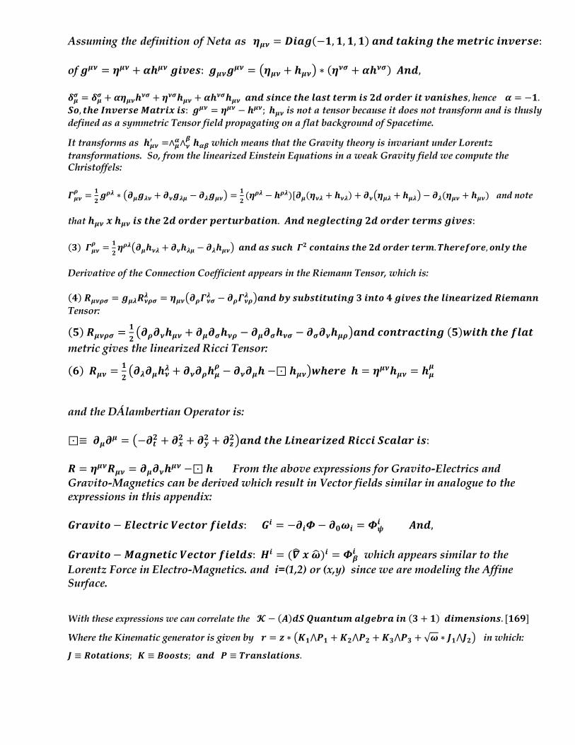
Assuming the definition of Neta as 𝜼𝝁𝝂 = 𝑫𝒊𝒂𝒈(−𝟏, 𝟏, 𝟏, 𝟏)𝒂𝒏𝒅𝒕𝒂𝒌𝒊𝒏𝒈𝒕𝒉𝒆𝒎𝒆𝒕𝒓𝒊𝒄𝒊𝒏𝒗𝒆𝒓𝒔𝒆: of𝒈𝝁𝝂 = 𝜼𝝁𝝂 + 𝜶𝒉𝝁𝝂𝒈𝒊𝒗𝒆𝒔:𝒈𝝁𝝂𝒈𝝁𝝂 = j𝜼𝝁𝝂 + 𝒉𝝁𝝂k ∗ (𝜼𝝂𝝈 + 𝜶𝒉𝝂𝝈)𝑨𝒏𝒅, 𝜹𝝁𝝈 = 𝜹𝝁𝝈 + 𝜶𝜼𝝁𝝂𝒉𝝂𝝈 + 𝜼𝝂𝝈𝒉𝝁𝝂 + 𝜶𝒉𝝂𝝈𝒉𝝁𝝂𝒂𝒏𝒅𝒔𝒊𝒏𝒄𝒆𝒕𝒉𝒆𝒍𝒂𝒔𝒕𝒕𝒆𝒓𝒎𝒊𝒔𝟐𝒅𝒐𝒓𝒅𝒆𝒓𝒊𝒕𝒗𝒂𝒏𝒊𝒔𝒉𝒆𝒔,hence 𝜶 = −𝟏. 𝑺𝒐, 𝒕𝒉𝒆𝑰𝒏𝒗𝒆𝒓𝒔𝒆𝑴𝒂𝒕𝒓𝒊𝒙𝒊𝒔:𝒈𝝁𝝂 = 𝜼𝝁𝝂 − 𝒉𝝁𝝂; 𝒉𝝁𝝂is not a tensor because it does not transform and is thusly defined as a symmetric Tensor field propagating on a flat background of Spacetime.
It transforms as 𝒉𝝁𝝂K =∧𝝁𝜶∧𝝂𝜷 𝒉𝜶𝜷which means that the Gravity theory is invariant under Lorentz
transformations. So, from the linearized Einstein Equations in a weak Gravity field we compute the Christoffels: 𝜞𝝁𝝂𝝆 = 𝟏
𝟐𝒈𝝆𝝀 ∗ k𝝏𝝁𝒈𝝀𝝂 + 𝝏𝝂𝒈𝝀𝝁 − 𝝏𝝀𝒈𝝁𝝂l =
𝟏𝟐(𝜼𝝆𝝀 − 𝒉𝝆𝝀)[𝝏𝝁(𝜼𝝂𝝀 + 𝒉𝝂𝝀) + 𝝏𝝂k𝜼𝝁𝝀 + 𝒉𝝁𝝀l − 𝝏𝝀(𝜼𝝁𝝂 + 𝒉𝝁𝝂) and note
that 𝒉𝝁𝝂𝒙𝒉𝝁𝝂𝒊𝒔𝒕𝒉𝒆𝟐𝒅𝒐𝒓𝒅𝒆𝒓𝒑𝒆𝒓𝒕𝒖𝒓𝒃𝒂𝒕𝒊𝒐𝒏.𝑨𝒏𝒅𝒏𝒆𝒈𝒍𝒆𝒄𝒕𝒊𝒏𝒈𝟐𝒅𝒐𝒓𝒅𝒆𝒓𝒕𝒆𝒓𝒎𝒔𝒈𝒊𝒗𝒆𝒔: (𝟑)𝜞𝝁𝝂
𝝆 = 𝟏𝟐𝜼𝝆𝝀k𝝏𝝁𝒉𝝂𝝀 + 𝝏𝝂𝒉𝝀𝝁 − 𝝏𝝀𝒉𝝁𝝂l𝒂𝒏𝒅𝒂𝒔𝒔𝒖𝒄𝒉𝜞𝟐𝒄𝒐𝒏𝒕𝒂𝒊𝒏𝒔𝒕𝒉𝒆𝟐𝒅𝒐𝒓𝒅𝒆𝒓𝒕𝒆𝒓𝒎. 𝑻𝒉𝒆𝒓𝒆𝒇𝒐𝒓𝒆, 𝒐𝒏𝒍𝒚𝒕𝒉𝒆
Derivative of the Connection Coefficient appears in the Riemann Tensor, which is: (𝟒)𝑹𝝁𝝂𝝆𝝈 = 𝒈𝝁𝝀𝑹𝝂𝝆𝝈𝝀 = 𝜼𝝁𝝂�𝝏𝝆𝜞𝝂𝝈𝝀 − 𝝏𝝆𝜞𝝂𝝆𝝀 �𝒂𝒏𝒅𝒃𝒚𝒔𝒖𝒃𝒔𝒕𝒊𝒕𝒖𝒕𝒊𝒏𝒈𝟑𝒊𝒏𝒕𝒐𝟒𝒈𝒊𝒗𝒆𝒔𝒕𝒉𝒆𝒍𝒊𝒏𝒆𝒂𝒓𝒊𝒛𝒆𝒅𝑹𝒊𝒆𝒎𝒂𝒏𝒏 Tensor:
(𝟓)𝑹𝝁𝝂𝝆𝝈 =𝟏𝟐j𝝏𝝆𝝏𝝂𝒉𝝁𝝂 + 𝝏𝝁𝝏𝝈𝒉𝝂𝝆 − 𝝏𝝁𝝏𝝈𝒉𝝂𝝈 − 𝝏𝝈𝝏𝝂𝒉𝝁𝝆k𝒂𝒏𝒅𝒄𝒐𝒏𝒕𝒓𝒂𝒄𝒕𝒊𝒏𝒈(𝟓)𝒘𝒊𝒕𝒉𝒕𝒉𝒆𝒇𝒍𝒂𝒕
metric gives the linearized Ricci Tensor:
(𝟔)𝑹𝝁𝝂 =𝟏𝟐j𝝏𝝀𝝏𝝁𝒉𝝂𝝀 + 𝝏𝝂𝝏𝝆𝒉𝝁
𝝆 − 𝝏𝝂𝝏𝝁𝒉 −⊡ 𝒉𝝁𝝂k𝒘𝒉𝒆𝒓𝒆𝒉 = 𝜼𝝁𝝂𝒉𝝁𝝂 = 𝒉𝝁𝝁
and the DÁlambertian Operator is: ⊡≡𝝏𝝁𝝏𝝁 = j−𝝏𝒕𝟐 + 𝝏𝒙𝟐 + 𝝏𝒚𝟐 + 𝝏𝒛𝟐k𝒂𝒏𝒅𝒕𝒉𝒆𝑳𝒊𝒏𝒆𝒂𝒓𝒊𝒛𝒆𝒅𝑹𝒊𝒄𝒄𝒊𝑺𝒄𝒂𝒍𝒂𝒓𝒊𝒔: 𝑹 = 𝜼𝝁𝝂𝑹𝝁𝝂 = 𝝏𝝁𝝏𝝂𝒉𝝁𝝂 −⊡𝒉 From the above expressions for Gravito-Electrics and Gravito-Magnetics can be derived which result in Vector fields similar in analogue to the expressions in this appendix: 𝑮𝒓𝒂𝒗𝒊𝒕𝒐 − 𝑬𝒍𝒆𝒄𝒕𝒓𝒊𝒄𝑽𝒆𝒄𝒕𝒐𝒓𝒇𝒊𝒆𝒍𝒅𝒔:𝑮𝒊 = −𝝏𝒊𝜱− 𝝏𝟎𝝎𝒊 = 𝜱𝝍
𝒊 𝑨𝒏𝒅, 𝑮𝒓𝒂𝒗𝒊𝒕𝒐 −𝑴𝒂𝒈𝒏𝒆𝒕𝒊𝒄𝑽𝒆𝒄𝒕𝒐𝒓𝒇𝒊𝒆𝒍𝒅𝒔:𝑯𝒊 = (𝜵"𝒙𝝎�)𝒊 = 𝜱𝜷
𝒊 which appears similar to the
Lorentz Force in Electro-Magnetics. and i=(1,2) or (x,y) since we are modeling the Affine Surface.
With these expressions we can correlate the 𝓚− (𝑨)𝒅𝑺𝑸𝒖𝒂𝒏𝒕𝒖𝒎𝒂𝒍𝒈𝒆𝒃𝒓𝒂𝒊𝒏(𝟑 + 𝟏)𝒅𝒊𝒎𝒆𝒏𝒔𝒊𝒐𝒏𝒔. [𝟏𝟔𝟗]
Where the Kinematic generator is given by 𝒓 = 𝒛 ∗ �𝑲𝟏⋀𝑷𝟏 +𝑲𝟐⋀𝑷𝟐 +𝑲𝟑⋀𝑷𝟑 + √𝝎 ∗ 𝑱𝟏⋀𝑱𝟐� in which:
𝑱 ≡ 𝑹𝒐𝒕𝒂𝒕𝒊𝒐𝒏𝒔; 𝑲 ≡ 𝑩𝒐𝒐𝒔𝒕𝒔; 𝒂𝒏𝒅𝑷 ≡ 𝑻𝒓𝒂𝒏𝒔𝒍𝒂𝒕𝒊𝒐𝒏𝒔.
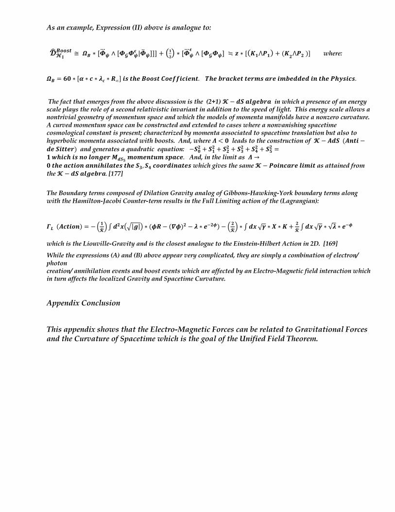
As an example, Expression (II) above is analogue to: 𝓓"𝓗∥
𝑩𝒐𝒐𝒔𝒕 ≅ 𝜴𝑩 ∗ [�⃛�𝝍 ∧ [𝜱𝓖𝜱𝝍𝝐 |�̈�𝝍]]] + j𝟏𝟐k ∗ [�⃛�𝝍
𝝐 ∧ [𝜱𝓖𝜱𝝍] ≒ 𝒛 ∗ [(𝑲𝟏⋀𝑷𝟏) + (𝑲𝟐⋀𝑷𝟐)] where:
𝜴𝑩 = 𝟔𝟎 ∗ [𝜶 ∗ 𝒄 ∗ 𝝀𝒄 ∗ 𝑹∞]𝒊𝒔𝒕𝒉𝒆𝑩𝒐𝒐𝒔𝒕𝑪𝒐𝒆𝒇𝒇𝒊𝒄𝒊𝒆𝒏𝒕.𝑻𝒉𝒆𝒃𝒓𝒂𝒄𝒌𝒆𝒕𝒕𝒆𝒓𝒎𝒔𝒂𝒓𝒆𝒊𝒎𝒃𝒆𝒅𝒅𝒆𝒅𝒊𝒏𝒕𝒉𝒆𝑷𝒉𝒚𝒔𝒊𝒄𝒔.
The fact that emerges from the above discussion is the (2+1) 𝓚−𝒅𝑺𝒂𝒍𝒈𝒆𝒃𝒓𝒂 in which a presence of an energy scale plays the role of a second relativistic invariant in addition to the speed of light. This energy scale allows a nontrivial geometry of momentum space and which the models of momenta manifolds have a nonzero curvature. A curved momentum space can be constructed and extended to cases where a nonvanishing spacetime cosmological constant is present; characterized by momenta associated to spacetime translation but also to hyperbolic momenta associated with boosts. And, where 𝜦 < 𝟎 leads to the construction of 𝓚−𝑨𝒅𝑺(𝑨𝒏𝒕𝒊 −𝒅𝒆𝑺𝒊𝒕𝒕𝒆𝒓) and generates a quadratic equation: −𝑺𝟎𝟐 + 𝑺𝟏𝟐 + 𝑺𝟐𝟐 + 𝑺𝟑𝟐 + 𝑺𝟒𝟐 + 𝑺𝟓𝟐 =𝟏𝒘𝒉𝒊𝒄𝒉𝒊𝒔𝒏𝒐𝒍𝒐𝒏𝒈𝒆𝒓𝑴𝒅𝑺𝟓 𝒎𝒐𝒎𝒆𝒏𝒕𝒖𝒎𝒔𝒑𝒂𝒄𝒆. And, in the limit as 𝜦 →𝟎𝒕𝒉𝒆𝒂𝒄𝒕𝒊𝒐𝒏𝒂𝒏𝒏𝒊𝒉𝒊𝒍𝒂𝒕𝒆𝒔𝒕𝒉𝒆𝑺𝟑, 𝑺𝟒𝒄𝒐𝒐𝒓𝒅𝒊𝒏𝒂𝒕𝒆𝒔 which gives the same 𝓚−𝑷𝒐𝒊𝒏𝒄𝒂𝒓𝒆𝒍𝒊𝒎𝒊𝒕 as attained from the 𝓚−𝒅𝑺𝒂𝒍𝒈𝒆𝒃𝒓𝒂. [177]
The Boundary terms composed of Dilation Gravity analog of Gibbons-Hawking-York boundary terms along with the Hamilton-Jacobi Counter-term results in the Full Limiting action of the (Lagrangian):
𝜞𝑳(𝑨𝒄𝒕𝒊𝒐𝒏) = −J𝟏𝓚XK∫𝒅𝟐𝒙k§|𝒈|l ∗ (𝝓𝑹 − (𝜵𝝓)𝟐 − 𝝀 ∗ 𝒆E𝟐𝝓) − J𝟐𝓚XK ∗ ∫𝒅𝒙√𝜸 ∗ 𝑿 ∗ 𝑲 +
𝟐𝓚X ∫𝒅𝒙√𝜸 ∗ √𝝀 ∗ 𝒆
E𝝓 which is the Liouville-Gravity and is the closest analogue to the Einstein-Hilbert Action in 2D. [169]
While the expressions (A) and (B) above appear very complicated, they are simply a combination of electron/ photon creation/ annihilation events and boost events which are affected by an Electro-Magnetic field interaction which in turn affects the localized Gravity and Spacetime Curvature.
Appendix Conclusion This appendix shows that the Electro-Magnetic Forces can be related to Gravitational Forces and the Curvature of Spacetime which is the goal of the Unified Field Theorem.
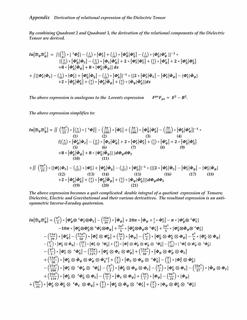
Appendix Derivation of relational expression of the Dielectric Tensor
By combining Quadrant 2 and Quadrant 3, the derivation of the relational components of the Dielectric Tensor are derived.
𝒍𝒏d𝓓𝝍𝓓𝝍r i ≃ ∫[a𝟏𝟒b ∗ [ 𝜱𝓔
𝟐] − � 𝟏𝟏𝟎� ∗ d�̇�𝓔𝝐 i + � 𝟏𝟏𝟎� ∗ d𝜱𝝍
𝟐 g�̇�𝓖𝝐 i − � 𝟏𝟏𝟎� ∗ [�̇�𝓖
𝝐𝝐 |�̇�𝝍𝝐 ]]:𝟏 ∗
[� 𝝅𝟐𝟓� ∗ d�̇�𝝍𝝐 g�̇�𝓔i − � 𝝅𝟐𝟓� ∗ d𝜱𝓔g�̈�𝝍
𝝐 i + 𝟐 ∗ d𝜱𝓔𝝐 g�̇�𝓔
𝝐 i + �𝟏𝟓� ∗ d�̇�𝝍𝝐 i + 𝟐 ∗ d𝜱𝓖
𝝐 g�̇�𝓖𝝐 i
+𝟖 ∗ d�̇�𝓖𝝐 g�̈�𝝍i + 𝟖 ∗ [𝜱𝓖
𝝐 |𝜱�𝝍]]𝒅𝒔
+∫[[𝜱𝓔𝝐 |�̇�𝓔] − � 𝟏𝟓𝟎� ∗ [𝜱𝓔
𝝐 ] + d𝜱𝓖𝝐 g�̇�𝓖i − � 𝟏𝟓𝟎� ∗ d𝜱𝓖
𝝐 i]:𝟏 ∗ [[𝟐 ∗ d�̇�𝓔𝝐 g�̈�𝓔i − d�̇�𝓔
𝝐 g�̇�𝝍i − [𝜱𝓔𝝐 |�̈�𝝍]
+𝟐 ∗ d�̇�𝓖𝝐 g�̈�𝓖
𝝐 i + �𝝅𝟑� ∗ d𝜱𝓖𝝐 g𝜱�𝝍i + �𝝅𝟑� ∗ [�̇�𝝍|�̈�𝓖
𝝐 ]]𝒅𝒔
The above expression is analogous to the Lorentz expression 𝑭𝝁𝝂𝑭𝝁𝝂 =𝑬𝟐 −𝑩𝟐.
The above expression simplifies to:
𝒍𝒏d𝓓𝝍𝓓𝝍r i ≈ ∬ a𝟒𝝅
𝟐
𝟐𝟓b ∗ d� 𝝅𝟔𝟑� ∗ [ 𝜱𝝐 𝓔
𝟐i − a 𝟑𝝅𝟏𝟎𝟎b ∗ d�̇�𝓔
𝝐 i + a 𝟑𝝅𝟏𝟎𝟎b ∗ d𝜱𝝍
𝟐 g�̇�𝓖𝝐 i − a 𝟑𝝅
𝟏𝟎𝟎b ∗ d�̇�𝓖
𝝐 g�̇�𝝍𝜺 i]:𝟏 ∗
(1) (2) (3) (4) {[� 𝝅𝟐𝟓� ∗ d�̇�𝝍
𝝐 g�̇�𝓔i − � 𝝅𝟐𝟓� ∗ d𝜱𝓔g�̈�𝝍𝝐 i + 𝟐 ∗ d𝜱𝓔
𝝐 g�̇�𝓔𝝐 i + �𝟏𝟓� ∗ d�̇�𝝍
𝝐 i + 𝟐 ∗ d𝜱𝓖𝝐 g�̇�𝓖
𝝐 i (5) (6) (7) (8) (9) +𝟖 ∗ d�̇�𝓖
𝝐 g�̈�𝝍i + 𝟖 ∗ [𝜱𝓖𝝐 |𝜱�𝝍]]}𝒅𝜱𝝍𝒅𝜱𝓔
(10) (11)
+∬ a𝟒𝝅𝟐
𝟐𝟓b ∗ [[𝜱𝓔
𝝐 |�̇�𝓔] − � 𝝅𝟏𝟓𝟕� ∗ [𝜱𝓔
𝝐 ] + d𝜱𝓖𝝐 g�̇�𝓖i − � 𝝅
𝟏𝟓𝟕� ∗ d𝜱𝓖𝝐 i]:𝟏 ∗ {[[𝟐 ∗ d�̇�𝓔
𝝐 g�̈�𝓔i − d�̇�𝓔𝝐 g�̇�𝝍i − [𝜱𝓔
𝝐 |�̈�𝝍] (12) (13) (14) (15) (16) (17) (18) +𝟐 ∗ d�̇�𝓖
𝝐 g�̈�𝓖𝝐 i + �𝝅𝟑� ∗ d𝜱𝓖
𝝐 g𝜱�𝝍i + �𝝅𝟑� ∗ [�̇�𝝍|�̈�𝓖𝝐 ]]}𝒅𝜱𝝍𝒅𝜱𝓔
(19) (20) (21)
The above expression becomes a quit complicated double integral of a quotient expression of Tensors; Dielectric, Electric and Gravitational and their various derivatives. The resultant expression is an anti-symmetric Inverse-Faraday quaternion.
𝒍𝒏d𝓓𝝍𝓓𝝍r i ≃ a𝝅
𝟐
𝟓b ∗ d𝜱𝝍
𝝐⨂ 𝜱𝓔⋆𝝐 ⨂�̇�𝓔i − a
𝟐𝟓𝝅𝟑𝟗b ∗ d�̇�𝝍i + 𝟐𝟎𝝅 ∗ d𝜱𝝍 + 𝟏
𝟐 ∗ �̇�𝓔𝝐 i − 𝝅 ∗ [𝜱𝝍
𝝐⨂ 𝜱𝝐 𝓔⋆ ]
−𝟏𝟎𝝅 ∗ d𝜱𝓖𝝐⨂�̇�𝓖
𝝐⨂ 𝜱𝝐 𝓔⋆⨂𝜱𝝍i +
𝟐𝝅𝟓
𝟓∗ d�̇�𝓖
𝝐⨂�̇�𝝍⨂ 𝜱𝝐 𝓔⋆i + 𝟐𝝅𝟓
𝟓∗ [𝜱𝓖
𝝐⨂�̈�𝝍⨂ 𝜱𝝐 𝓔⋆ ]
−a𝟏𝟏𝝅𝟑𝟗b ∗ d�̇�𝝍
𝝐 i − a𝟐𝟕𝝅𝟒
𝟓𝟎b ∗ d𝜱𝓔
𝟐⊗𝜱𝝍𝝐 i + a𝟑𝝅
𝟓b ∗ d𝜱𝝍i − a
𝝅𝟒
𝟓b ∗ d𝜱𝓖
𝝐 ⊗ �̇�𝓖𝝐 ⊗𝜱𝝍i −
𝝅𝟓
𝟒∗ [�̇�𝓖
𝝐 ⊗ �̇�𝝍]
−O𝝅𝟓
𝟒P ∗ e𝜱𝓖
𝝐 ⊗�̈�𝝍f − O𝟐𝝅𝟑P ∗ e𝜱𝓔
𝝐 ⊗ 𝜱𝓖⋆𝝐 f + O𝝅𝟑P ∗ e𝜱𝓔
𝟐⊗�̇�𝝍𝝐 ⊗𝜱𝝍
⋆ ⊗ �̇�𝓖⋆𝜺 f − O𝝅
𝟒
𝟏𝟎P ∗ [ 𝜱𝝐 𝓔
𝟐⊗𝜱𝝍⋆ ⊗ �̇�𝝐 𝓖
⋆ ]
−a𝝅𝟐
𝟑b ∗ d𝜱𝓔
𝝐 ⊗ �̇�𝝐 𝓖⋆ i − a𝟐𝟓𝝅
𝟏𝟏𝟕b ∗ d𝜱𝓖
𝝐 ⊗𝜱𝓔⊗𝜱𝝍⋆ i + a𝟏𝟏𝝅
𝟓
𝟓𝟎b ∗ d�̇�𝝍⊗𝜱𝝍
⋆ ⊗𝜱𝓔i
+a𝟏𝟏𝝅𝟓
𝟓𝟎b ∗ d𝜱𝓖
𝝐 ⊗ �̈�𝝍⊗𝜱𝝍⋆ ⊗ �̇�𝓖
:𝝐i + a𝝅𝟑b ∗ d𝜱𝓔⊗𝜱𝝍⊗ �̇�𝝐 𝓖
⋆ i − a𝝅𝟑b ∗ [𝜱𝓔
𝟐⊗ �̇�𝓖𝝐 ]
−a𝟐𝟕𝝅𝟐
𝟐𝟎𝟎b ∗ d𝜱𝓔
𝝐 ⊗ 𝜱𝝐 𝝍⋆ ⊗ 𝜱𝝐 𝓖
⋆ i − a𝝅𝟐
𝟑b ∗ d�̇�𝓖
𝝐 ⊗𝜱𝝍⊗𝜱𝓔i − a𝝅𝟒
𝟑b ∗ d𝜱𝓖
𝝐 ⊗𝜱𝓔i − a𝟐𝟓𝝅𝟓
𝟓𝟕b ∗ [�̈�𝝍⊗𝜱𝓔]
+a𝟐𝟓𝝅𝟓
𝟏𝟏𝟒b ∗ d𝜱𝓖
𝝐 ⊗ �̇�𝝐 𝓖⋆ ⊗𝜱𝓔i − a
𝟒𝝅𝟕b ∗ d�̇�𝓔⊗𝜱𝝍i + a
𝟐𝝅𝟕b ∗ d𝜱𝝍i − a
𝟒𝝅𝟐
𝟐𝟓b ∗ [�̇�𝝍]
+a𝟖𝝅𝟐
𝟐𝟓b ∗ d�̇�𝓖
𝝐 ⊗ �̈�𝓖𝝐 ⊗ 𝜱𝝐 𝓔 ⊗𝜱𝝍i + a
𝝅𝟐b ∗ d𝜱𝓖
𝝐 ⊗ �̈�𝝍⊗ 𝜱𝓔⋆𝝐 i + a𝝅
𝟐b ∗ [𝜱𝝍⊗ �̈�𝓖
𝝐 ⊗ 𝜱𝜺 𝓔⋆ ]

−a𝟗𝝅𝟒
𝟏𝟎b ∗ d𝜱𝓔
𝝐 ⊗ �̇�𝓔⊗𝜱𝝍i − a𝟐𝟓𝝅𝟒
𝟓𝟒b ∗ d𝜱𝓔
𝝐 ⊗𝜱𝝍i + 𝟖𝝅𝟐 ∗ d𝜱𝓔⊗ �̇�𝝍i − a𝟗𝝅𝟒
𝟏𝟎b ∗ [�̇�𝓖
𝝐 ⊗ �̈�𝓖𝝐 ⊗𝜱𝝍]
−𝟏𝟓𝝅 ∗ d𝜱𝓖𝝐 ⊗ �̈�𝝍i + 𝟏𝟓𝝅 ∗ d�̈�𝓖
𝝐 ⊗𝜱𝝍i + 𝝅 ∗ [𝜱𝓔𝝐 ⊗ �̇�𝓔⊗ 𝜱𝝐 𝓖
⋆ ⊗ �̇�𝓖⋆ ⊗𝜱𝝍]
−a𝝅𝟐b ∗ d𝜱𝓔
𝝐 ⊗𝜱𝝍⊗ 𝜱𝝐 𝓖⋆ ⊗ �̇�𝓖
⋆ i − (a𝟒𝝅𝟐
𝟐𝟓b ∗ [ 𝜱𝝐 𝓔
𝟐⊗ �̇�𝝍⊗ 𝜱𝝐 𝓖⋆ ⊗ �̇�𝓖
⋆ ]
+a𝟖𝝅𝟐
𝟐𝟓b ∗ d�̈�𝓖
𝝐 ⊗𝜱𝓖⋆ ⊗𝜱𝝍⊗𝜱𝓔i + a
𝝅𝟐b ∗ d�̈�𝝍⊗ �̇�𝓖
⋆ ⊗𝜱𝓔i + a𝝅𝟐b ∗ [𝜱𝝍⊗ �̈�𝓖
𝝐 ⊗ 𝜱𝝐 𝓖⋆ ⊗ �̇�𝓖
⋆ ⊗𝜱𝓔] −𝟏𝟔𝝅𝟐 ∗ d𝜱𝓔
𝝐 ⊗ �̇�𝓔⊗ 𝜱𝝐 𝓖⋆ ⊗𝜱𝝍i − 𝟖𝝅𝟐 ∗ d𝜱𝓔
𝝐 ⊗𝜱𝝍⊗ 𝜱𝝐 𝓖⋆ i + 𝟒𝝅𝟐 ∗ [𝜱𝓔
𝟐⊗ �̇�𝝍𝝐 ⊗ 𝜱𝝐 𝓖
⋆ ]
−𝟏𝟔𝝅𝟐 ∗ d�̇�𝓖𝝐 ⊗ �̈�𝓖
𝝐 ⊗𝜱𝓖⋆ ⊗𝜱𝝍
𝝐 ⊗𝜱𝓔i − a𝟐𝟎𝝅𝟒
𝟓𝟗b ∗ d�̈�𝝍⊗𝜱𝓔i − a
𝟐𝟎𝝅𝟒
𝟓𝟗b ∗ [𝜱𝝍⊗ �̈�𝓖
𝝐 ⊗𝜱𝓖⋆ ⊗𝜱𝓔
𝝐 ]
Note: 𝑻𝒉𝒆𝒕𝒆𝒓𝒎𝒔𝜱⋆𝒂𝒓𝒆𝒕𝒉𝒆𝒊𝒏𝒗𝒆𝒓𝒔𝒆𝒇𝒖𝒏𝒄𝒕𝒊𝒐𝒏𝒔𝒐𝒇𝜱𝒘𝒉𝒆𝒓𝒆𝜱 = 𝟏. 𝟔𝟏𝟖𝒂𝒏𝒅𝜱⋆ =. 𝟔𝟏𝟖𝒂𝒏𝒅 are Relational Factors of the applicable Tensor; Dielectric, Electric, and Gravitational.
Since the above expression is analogue to 𝑭𝝁𝝂𝑭𝝁𝝂 =𝑬𝟐 −𝑩𝟐 the expression can be rewritten in that the
𝜱𝝍⊗𝜱𝓔 ≈𝜱𝜷𝒕𝒉𝒆𝑴𝒂𝒈𝒏𝒆𝒕𝒊𝒄𝒇𝒊𝒆𝒍𝒅. While the above expression shows how complicated the Dielectric Vacuum can be, it must also be remembered that the Dielectric Vacuum field through loss of inertia and in the presence of gravitational forces (caused from Centripetal forces) gives birth to Neutrons which later decay to a Proton, electron and photon.
The Dielectric Vacuum is composed of incommensurate energetic particles which through interactions via collisions amongst themselves and gravitational effects can create real particles. In recent research, it has been hypothesized that (Sept. 2010), that Dark Matter is modeled by vortices in Bose-Einstein Condensate Dark Matter. Through analysis of theoretical vortices dark matter is characterized as Bosons (similar to X-17 previously discussed), with boson mass is centered around 𝒎~𝟏𝟎:𝟔𝟎 − 𝟏𝟎:𝟓𝟖𝒌𝒈𝒐𝒓𝟏𝟎:𝟐𝟒 − 𝟏𝟎:𝟐𝟐𝒆𝑽 with a vortex radius 𝑹𝒗𝒐𝒓~𝟏𝟎𝟐𝟎 −𝟏𝟎𝟐𝟏𝒎. [210] It is clear to see that this boson mass is much less than that of the electron 9.109390 (𝟏𝟎:𝟑𝟏)and the Neutrino 𝟏. 𝟓(𝟏𝟎:𝟑𝟔)𝒌𝒈 and does not interact with other observable particles except through Gravitational effects (Halos) and through effecting baryonic resonances.
Returning to the combining of Quadrant 2 with 3 of Volume II, Attachment A, Figure 1; the expression for the Dielectric Vacuum Energy at the Landau-Zener Zero-line becomes:
(𝑰)∆𝑬𝟐≈ (𝟐𝝅
𝟑
𝟓) ∗ j𝒄∗𝒉∗𝑮
𝜶∗𝝀𝒄m ∗ cd𝜱𝓖
𝟐 ⊗𝜱𝝍𝝐⨂�̇�𝝍
𝝐 i − a 𝟑𝟏𝟔b ∗ d𝜱𝓖
𝝐⨂𝜱𝝍𝟐⨂�̇�𝝍il
Of note is that the Energy is dominated by Angular Momentum terms which supports the conclusions in reference [210]. Therefore:
∫𝒅𝟑𝒓 ∗ a𝟏𝟐𝒗𝟐 + j 𝑽𝟎
𝟐𝒎𝟐 ∗ 𝝆m +𝟏𝟐𝑽𝑮b ∗ 𝝆 ≅ (
𝟐𝝅𝟑
𝟓) ∗ j𝒄∗𝒉∗𝑮
𝜶∗𝝀𝒄m ∗ cd𝜱𝓖
𝟐 ⊗𝜱𝝍𝝐⨂�̇�𝝍
𝝐 i − a 𝟑𝟏𝟔b ∗ d𝜱𝓖
𝝐⨂𝜱𝝍𝟐⨂�̇�𝝍il [210]
Which is the Energy for a single asymmetric vortex.
Appendix Conclusion
It has been shown that an expression of the Dielectric Tensor can be derived which is analogue to the Inverse-Faraday effect thus describing the Dielectric Vacuum and Dark Matter/ Energy. Furthermore, an expression related to Energy of the Dark Matter Vortices can be derived.
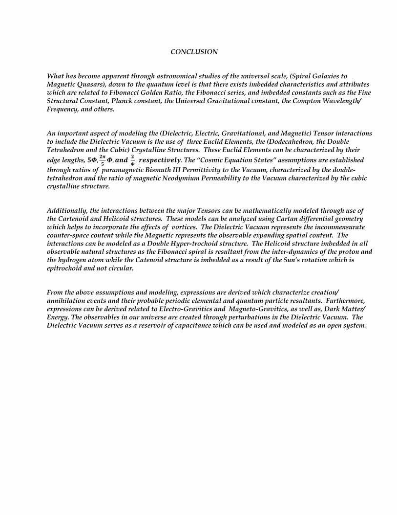
CONCLUSION
What has become apparent through astronomical studies of the universal scale, (Spiral Galaxies to Magnetic Quasars), down to the quantum level is that there exists imbedded characteristics and attributes which are related to Fibonacci Golden Ratio, the Fibonacci series, and imbedded constants such as the Fine Structural Constant, Planck constant, the Universal Gravitational constant, the Compton Wavelength/ Frequency, and others.
An important aspect of modeling the (Dielectric, Electric, Gravitational, and Magnetic) Tensor interactions to include the Dielectric Vacuum is the use of three Euclid Elements, the (Dodecahedron, the Double Tetrahedron and the Cubic) Crystalline Structures. These Euclid Elements can be characterized by their edge lengths, 𝟓𝜱, 𝟐𝝅
𝟓𝜱,𝒂𝒏𝒅 𝟐
𝜱𝒓𝒆𝒔𝒑𝒆𝒄𝒕𝒊𝒗𝒆𝒍𝒚. The “Cosmic Equation States” assumptions are established
through ratios of paramagnetic Bismuth III Permittivity to the Vacuum, characterized by the double-tetrahedron and the ratio of magnetic Neodymium Permeability to the Vacuum characterized by the cubic crystalline structure.
Additionally, the interactions between the major Tensors can be mathematically modeled through use of the Cartenoid and Helicoid structures. These models can be analyzed using Cartan differential geometry which helps to incorporate the effects of vortices. The Dielectric Vacuum represents the incommensurate counter-space content while the Magnetic represents the observable expanding spatial content. The interactions can be modeled as a Double Hyper-trochoid structure. The Helicoid structure imbedded in all observable natural structures as the Fibonacci spiral is resultant from the inter-dynamics of the proton and the hydrogen atom while the Catenoid structure is imbedded as a result of the Sun’s rotation which is epitrochoid and not circular.
From the above assumptions and modeling, expressions are derived which characterize creation/ annihilation events and their probable periodic elemental and quantum particle resultants. Furthermore, expressions can be derived related to Electro-Gravitics and Magneto-Gravitics, as well as, Dark Matter/ Energy. The observables in our universe are created through perturbations in the Dielectric Vacuum. The Dielectric Vacuum serves as a reservoir of capacitance which can be used and modeled as an open system.
REFERENCES
1. “Pushing Gravity”, ’New Perspectives on LeSage’s Theory of Gravity’; Georges-Louis LeSage (1724-1803); “Gravitation”, Matthew R. Edwards, 2002.
2. “Mach’s Principle and the Origin of Inertia”, M. Sachs and A. R. Roy, 2003. “DE Divina Proportione”, Loca Pacioli and Leonardo DaVinci, 1509.
3. "Differential Geometry”, ‘Cartan’s Generalization of Klein-Erlangen Program’, R.W. Sharpe, 1991.
4. “Asymptotic Methods”, ‘A Course in Mathematical Tripos’, Cambridge University, England, Richard Chapling, April 2016. 5. “Uncovering the Secrets of Magnetism”, Ken Wheeler, May 2014. 6. “General Relativistic Gravity Machine using ElectroMagneto-Torsion Field”, Taaki Musha, Mario J. Pinheiro; International Journal of Sciences, Vol. 7, March 2018(03). 7. “Publishing’s of DE Broglie, Einstein, Cartan, Vergie”; Paris Academy of Natural Philosophy, 1920s. 8. “Energy from the Vacuum”, ‘Concepts and Principles’; Lt. Col. Thomas E. Bearden, PhD, 2002. 9. “Quantum Gravity Research Overview”, Kevin Irwin, PhD, et al., May 2017. 10. “Mandelbrot Fractals, and Chaos Theory”, Carl Mandelbrot 11. “Rovelli’s Equation for Lower Bound of Black Hole Entropy’, Carl Rovelli, 2018. 12. “Writings of Aristotle and Fibonacci” 13. “Loop Quantum Gravity Parameter to a Black Hole Entropy”, Amaral. 14.“Poincare’s Disk Model for Hyperbolic Geometry”, Poincare, 1683. 15. “Time Emerges from Entanglement”, ‘Quantum Experiment’; Forteanna Forums; Don Page, Wm. Woeters. 16. “Lectures and Publishing’s”, Eric Wen der Verlinde. 17. “Giant Peak of the Inverse Faraday Effect in the band Gap of Magneto-photonic Microcavity” 18. “Brand New Phase of Matter Discovered by Scientists, ‘Time Crystals’; Chris Monroe, University of Maryland, Physics Journal, January 28, 2017. 19. “The Link Between the Sachs and O(3) Theories of ElectroDynamics. 20. “Stanford Lecture Series,” ‘Classical Mechanics, Quantum Mechanics, Quantum Entanglement, Black Holes’; Leonard Susskind. 21. “The Order of Time”, Carlo Rovelli, 2018. 22. “The Higgs Fake”, Alexander Unzicker, PhD. 23. “Poincare Asymptotics” Lecture Series; Perimeter Institute, Waterloo, Ontario, CA.; Carl Bender, Univ. of St. Louis, 2009. 24. “An Application of Gauge Theory to Four-Dimensional Topology”, S. K. Donaldson, Dec. 31, 1982. 25. “Principles of ECE Theory”, ‘A New Paradigm of Physics’; Myron W. Evans, Horst Eckardt, Douglas W Lindstrom, Stephen J. Crothers, Sept. 29, 2016. 26. “ECE Theory”, Laurence Felker 27. “Post Einsteinian Paradigm Shift”, Alwyn van der Merwe, PhD., Professor Emeritus, Univ. of Denver, 2007. 28. “ElectroMagnetic Force Density and Energy-Momentum Tensor in an Arbitrary Continuous Medium”, A. Shevchenko, M. Kaivola; Journal of Physics, 44(17), pp. 175401, 2011. 29. “Space and Time in Loop Quantum Gravity”, Carlo Rovelli, HAL-01714251, 20 April 2018. 30. “On the Origin of Gravity and the Laws of Newton”, Erik Verlinde, Jan. 2010. 31. “Surface Waves and the ‘Critical’ Propagation Experiment”, Wireless Power Conference, Mar. 2016. 32. “A Gravitational and Electromagnetic Analogy”, Oliver Heaviside, Part I, ‘The Electrician’, 31, pp. 281-282; 1893. 33. “The Incommensurability of Scientific Theories”, Stanford Encyclopedia of Philosophy. 34. “From Planck Data to Planck Era: Observational tests of Holographic Cosmology”, Niayesh Afshordi, Claudio Corian, et al.; Perimeter Institute for Physics; Waterloo, Ca., Jan. 2017. Also, See Ref. [80-83].
35. “Simplified Derivation of the Hawking-Unruh Temperature for an Accelerated Observer in Vacuum”, Paul M. Ashley, Peter W. Milonni, Feb. 2008. 36. “The R spectra of atoms and molecules” Journal of Physics and Chemistry, M W Evans, H Eckards, 2011, vol. 1 (2) 176 - 185. 37. “The Covariant mass ratio of Einstein-Cartan-Evans Theory”, Journal of Physics and Chemistry, M W Evans, H Eckardt 2011 vol. 1,158-167. 38. “The Golden Ratio”, ‘The Divine Beauty of Mathematics’, Gary B. Meizner. 39. “Euclid Elements”, Euclid.
40. “Electricity and Matter”, J. J. Thomson, Cambridge, Aug. 1903. 41. “Ether Technology”, ‘A Rational Approach to Gravity Control’, Rho Sigma, 1997. 42. Hexagons on Jupiter and Neptune, https://truestrange.com/2018/05/31/jupiters-octagon-and-pentagon-shaped-cyclones/ 43. Pentagons on Earth and Saturn, https://eoimages.gsfc.nasa.gov/images/imagerecords/59000/59758/SouthAtlantic.A2002157.1055.500m.jpg 44. Stoyan Sarg "A Physical Model of the Electron according to the Basic Structures of Hypothesis, Physics Essays, vol. 16 No. 2,180-195, (2003); http://www.physicsessays.com 45. S. Sarg, Basic Structures of Matter-Supergravitation Unified Theory, Trafford Publishing, 2006, ISBN 1412083877 (books review in "Physics in Canada," v. 62, No. 4, July/Aug 2006. 46. S. Sarg, BSM-Supergravitation Unified Theory based on an alternative Concept of the Physical Vacuum, IX Int. Sci. Conf. "Matter, Energy, Gravitation," 7-11 Aug 2006, St. Petersburg, Russia. 47. S. Sarg, BSM Supergravitation Unified Theory, on a new concept of the Physical Vacuum. Major Predictions. Int. Conf. on Future Energy (COFE-2006) 22-24 Sep 2006, Washington D.C. 48. Stoyan Sarg, "Field Propulsion by Control of Gravity," 'Theory and Experiments' Copyright © 2009. 49. K. Pendergast, “Crystal Spheres”, www.aias,us. 50. Omnia Opera Section, www.aias.us. 51. H. Eckardt, “ECE Engineering Model”, http://www.aias.us/documents/miscellaneous/ECE-Eng-Model.pdf. 52. M. W. Evans, (ed.), “Modern Non-Linear Optics”, a special topical issue of I. Prigogine and S. A. Rice, “Advances in Chemical Physics”, (Wiley Interscience, New York, 2001, second edition), vols. 119(1) to 119(3). 53. M. W. Evans and S. Kielich (eds.), ibid., first edition (Wiley Interscience), New York, 1992, 1993, 1997), vols 85(1) to 85(3). 54. M. W. Evans and L. D. Crowell, “Classical and Quantum Electrodynamics and the B(3) Field” (World Scientific, 2001). 55. M W. Evans and J.-P. Vigier, “The Enigmatic Photon” (Kluwer, 1994 to 2002), in five volumes. 56. M. W. Evans and A. A. Hasmein, “The Photomagneton in Quantum Field Theory” (World Scientific, 1994). 57. “Santilli’s Isodual Mathematics and Physics for Anti-Matter”, P. M. Bhujbal, American Journal of Modern Physics, 2016; 5(2-1): 161-184 http://www.sciencepublishinggroup.com/j/ajmp doi:10.11648/j.ajmp.2016050201.20 ISSN: 2326-8867 (Print); ISSN: 2326-8891 (online). 58. Outline of Hadronic Mathematics, Mechanics and Chemistry as Conceived by R. M. Santilli; American Journal of Modern Physics, 2015; 4(5-1): 1-16; Published online: August 10, 2015 http://www.sciencepublishinggroup.com/j/ajmp doi:10.11648/j.ajmp.s.2015040501.11 ISSN:2326-8867 (Print); ISSN:2326-8891 (online). 59. M. W. Evans and H. Eckardt, “The R Spectra of atoms and molecules”, Alpha Institute for Advanced Studies (AISA) (www.aias.us); **(Unified Physics Institute of Technology (UPITEC) (www.upitec.org). 60. Carl Bender, PhD., Washington Univ. of St. Louis, “Lectures on Mathematical Physics”. 61. “Given 2 masses that have Gravitational Potential Energy between them, where is the Gravitational Potential Energy stored?” www.quora.com. 62. Harris E. G., Analogy between General Relativity and Electro-Magnetism for slowly moving particles in weak Gravitational Fields, American Journal of Physics, 59 (5), 1991, pp. 421-425. 63. Harpaz, A., Soker, N., ‘Radiation from a Uniformly Accelerated Charge, Gen. Rel. Grav. 30 (8), 1998, 1217-1227. 64. Huggins, Elisha, R., Exact Magnus-Force Formula for Three-Dimensional Fluid-Core Vortices, Phys. Rev. A 1 (2) 1970, 327-331. 65. Pinhero, Mario J., On Newton’s third law and its symmetry-breaking effects, Physica Scripta 84 (5), 2011, 055004.

66. Hedenstrom, Anders, A General Law for animal Locomotion, TRENDS in Ecology and Evolution 19(5), 2004, 217-219. 67. Robertson, G. A., Pinheiro, M.,” Vortex Formation in the Wake of Dark Matter Propulsion”, Physics Procedia, 20, 2011, 6-23. 68. Murad, P. A., “A proposed model for capturing gravitational spin anomalies”, Space Technology and Application International Forum (STAIF-2004), AIP conference proceedings 699, NY, American Institute of Physics, 2004, pp. 1090-1105. 69. Pinheiro, Mario J., “Some effects of Topological Torsion currents on Spacecraft dynamics and the flyby anomaly, Monthly Notices of the Royal Astronomical Society, Volume 461, Issue 4, 1 October 2016, Pages 3948-3953. 70. Pinheiro, Mario J., A reformulation of mechanics and electrodynamics, Heliyon 3 (2017) e00365. 71.”Incursion of the Golden Ratio Φ into the Schrödinger Wave function using the φ Recursive Heterodyning Set”, S. Giandinoto*, R. L. Amoroso§ & E.A. Rauscher*Advanced Laser Quantum Dynamics Research Institute (ALQDRI). 72. “Landau-Zener Damping Theory (1931)”, Interference, Harmonic Research and Theory, Filed 19/04/17, Harmonics and Physics. 73. “Cosmos Conversation Space”, Cosmos Magazine, 01 October 2018. earthchangesmedia.com 74. “Vectorization: Rothwild-O”, Unknown, provided by NASA and Hubble Heritage Team, earthchangesmedia.com . 75. “Resolved Structure of a Galactic active Nucleus”, Resonance; © 2008 Pearson Education, Inc.; earthchangesmedia.com . 76. “Massive ‘Ocean’ discovered towards Earth’s Core”, Earth, 12 June 2014; Newscientist.com, Journal Reference, Science, DOI: 101126/science.1253358. 77. “Neutron Star reveals the Energetic Nature of the Empty Vacuum”., Resonance, 24 Apr 2017; https://hiup.org/neutron-star-reveals-energetic-nature-empty-vacuum/ 78. A. Antognini, et al., “Proton Structure from the Measurement of 2S-2P Transition Frequencies of Muonic Hydrogen”, Science, vol. 339, (25 January 2013). 79. R. Pohl, A. Antognini, F. Nez, et al., “The size of the proton”, Nature, vol. 466, issue 7303, pp. 213-216 (2010). 80. N. Haramein, "Quantum Gravity and the Holographic Mass", Copyright, (20 December 2012). 81. Resonance Science Foundation, Resonance Digest, Sept. 20, 2019, “New Measurement of the Proton Charge Radius Confirms Nassim Haramein’s 2012 Prediction”. 82. N. Haramein, Patent US 8,073,094 B2, Dec. 6, 2011; “Device and Method for Simulation of Magneto-Hydrodynamics”. 83. Physics Essays, “Holographic Proton Mass Prediction”, Vol 32, pp. 255-262, Dec. 2019. 84. “Free Energy Generation”, Bedini-Bearden Years, 2d Edition, 2011. 85. “Reality is Not What it Seems”, The Journey to Quantum Gravity, Carlo Rovelli, Riverhead Books 2017. 86. “Sub-Quantum Kinetics”, A Systems Approach to Physics and Cosmology, Paul A. LaViolette ,Starlane Publications,1994. 87. “The Trouble with Physics”, The Rise of String Theory, the Fall of a Science, and What Comes Next, Lee Smolin, Mariner Books, 1st edition 2007. 88. “Three Roads to Quantum Gravity”, Lee Smolin, Basic Books, New York, NY; 2017 edition. 89. “Understanding Relativistic Quantum Field Theory”, Chapter 22, Hans de Vries, January 2, 2009. 90. Lord Kelvin, “On the Generation of Longitudinal Waves in Ether”, Proceedings of the Royal Society of London, 59, 270-273, (1895-1896). 91. C. Monstein and J. P. Wesley, “Observation of Scalar Longitudinal Electromagnetic Waves”, Electrophysics Letters, 59, (4), 514-520 (2002). 92. Massines et al., “Experimental and Theoretical study of a glow discharge at atmospheric pressure controlled by a Dielectric Barrier”, L. Appl. Physics 83, 2950 (1998). 93. H. Malhado, “Creative Common Zero”, https://commons.wkimedia.org/w/index.php?curd=29628137. 94.”High Speed Jets Spewing out of a Super-massive Blackhole”, Space.com; https://www.iflscience.com/space/relativistic-jets/ 95. “Dark Matter Space”, https://www.darkmatterspace.files.wordpress.com/ 96. Dr. R. M. Santilli Biographical Notes http://www.i-b-r.org/Dr-R-M-Santilli-Bio-1-10-18.pdf,Full Curriculum http://www.i-b-r.org/Ruggero-Maria-Santilli.htm, Awards and Nominations http://santilli-foundation.org/santilli-nobel-nominations.html.
97. Dr. R. M. Santilli Invited Plenary Lecture https://www.youtube.com/watch?v=eyS6HDO5xDc&feature=youtu.be at the Sustainable Industrial Processing Summit & Exhibition Hainan Island, China, November 6 to 10, 2016 http://www.flogen.org/sips2016 98. “The Mass of the Photon”, Liang-Cheng, Jun Luo, George T. Gillies; Inst. of Physics Publishing, Reports on Progress in Physics; 23 Nov. 2004; doi: 10.1088/0034-4885/68/1/R02; https://iopscience.iop.org/article/10.1088/0034-4885/68/1/R02
99. “The Rest Mass of a Photon”, Kamal l. Rajpal, Sept. 2013; http://vixra.org/pdf/1307.0094v2.pdf 100. J. Beringer et al. (Particle Data Group), PR D86, 010001 (2012); http://pdg.lbl.gov/2011/listings/rpp2011-list- photon.pdf 101. “The Unified Spacememory Network”, Haramein, et al.; NeuroQuantology, December 2016, Vol. 14, Issue 4,doi: 10.14704/ nq.2016.14.4.961. 102. “Astrophysical detection of the Helium hydride ion HeH+”, Rolf Gusten, Helmut Wiesemeyer, et al., Nature, 568, pp. 357-359; 2019
103. “Scale Unification: A Universal Scaling Law for Organized Matter”, N. Haramein, M. Hyson, E. A. Rauscher; Proceedings of the Unified Theories Conference, 2008. 104. Module 4, “Energy and Spin of a Proton”, Unified Physics, Resonancescience.org. 105. Module 4, “The Gravitational Coupling Constant”, Unified Physics, Resonancescience.org 106. Module 4, “Gravitational Falloff and the Yukawa Potential”, Unified Physics, Resonancescience.org 107. Anthony G. Holland, Novobiotronics Inc., Ted Talk (2013). 108. Christine Gibbons, CEO HistoSonics Inc., Ted Talk Feb. 27, 2017. 109. Dr. Lee Bartel, Univ. Toronto, “How Sound Impacts the Body”, Ted Talk,11/2017. 110. Kevin Orlowski, “Magnetic Energy”, BEM Conference, 2015; www.magneticenergy.org.uk 111. Image of the Nova Centauri Galaxy, image courtesy of ESO; eso1531a_Nova_Centauri.jpg 112. “Gravitational lensing reveals ionizing ultraviolet Photons escaping from a Distant Galaxy”, Science Magazine, Nov. 8, 2019. 113. Image of Sunburst Arc, Galaxy PSZ1 G311.6602-18.4624; spacetelescope.org, Nov. 13, 2019. 114. “Engineering spin-orbit synthetic Hamiltonians in Liquid-Crystal Optical Cavities”, Katarzyna Rechcin’ska, et al., Report: Topological Optics, Science Magazine, Nov. 8, 2019. 115. “Entropy Production in Open Systems: The Predominant Role of Intraenvironment Correlations”, Krzysztof Ptaszynski and Massimiliano Esposito, APS, Physical Review Letters; vol. 123, 200603, Nov. 13, 2019. 116. “A New Negative Ion takes the Cooling Spotlight”, Rulin Tang, et al.; APS, Physical Review Letters, vol. 123, 203002, Nov. 12, 2019.
117. “Physicists Claim they’ve found even more Evidence of a New Force of Nature”,
https://www.sciencealert.com, Article by Mike McRae, Nov. 20, 2019.
118. “Fifth Force”, Wikipedia; https://en.wikipedia.org/wiki/Fifth_force.
119. “Evidence for a Protophobic Fifth Force from ‘Be’ Nuclear Transitions”, Jonathan L. Feng, et al.; aiX1v:1604.0/411V1, 25 Apr. 2016; PACS No. 14.70.Pw, 27.20.+n, 21.30.-x, 12.60.Cu,13.60.-r
120. “The Rainbow and the Worm”, ‘The Physics of Organisms’, Mae-wa Ho, 3d Edition, Institute of Science in Society; World Scientific Publishing, 2008.
121. “A Graphene Waveguide for Electrons”, A. Cheng, J. Cheng, et al., Stanford Univ., https://physics.aps.org/articles/ vol. 12/132; November 22, 2019.
122. “A New form Carbon Dazzles and Attracts”, W. Wyat Gibbs, https://sciencemagazine.org/sciencemagazine/15_november_2019/
123. “First results from TNG50 simulation: the evolution of Stellar and Gaseous Discs across Cosmic Time”, Annalisa Pillepich, Dylan Nelson, et al., Royal Astronomical Society, MNRAS 490, 3196-3233(2019); Published by Oxford Univ. Press; 9 Sept. 2019.
124. “Black, Hot Ice may be Nature’s Most Common Form of Water”, Chemistry, ‘A New Experiment Confirms the Existence of “Superionic Ice”; Quantum Magazine, 11 Nov. 2019, https://www.quantummagazine.org/blavck-hot-superionic-ice-maybe-natures-most-common-form-of-water-20190508/
125. “New Type of Star System?”, The Conversation Magazine, 25 Nov. 2019; https://www.theconversation.com/new-type-of-star-system-radio-signal-puzzles-astronomers-127699/
126.”On Causality Proofs of Superluminal Barrier Transversal of Frequency Band Limited Wave Packets”, Phys. Lett. A196, 1994, pp. 154-158. And Enders, G. Nimtz, Phys. Lett., Vol. 48, 1993, pg. 632.
127. “The Speed of Gravity; What the Experiments Say”, Tom van Flandern, Phys. Lett., A, Vol. 250, 21 Dec. 1998, pp. 1-11.
128. D. J. Evans, Lamberto Rondoni, “Comments on the Entropy of Nonequilibrium Steady States”, J. Stat. Phys., 109(3-4), Nov. 2002, pp. 295-920.
129. Paul Davies, “Superforce: The Search for a Grand Unified Theory of Nature”, Simon and Schuster, New York, 1984, pg. 105.
130. M. W. Evans, “The link Between the Sachs and O(3) Theories of Electrodynamics”, in ‘Modern Nonlinear Optics’, Second Edition (3 Vols.), edited by Myron W. Evans, 2000; Advances in Chemical Physics, Wiley, New York, Ilya Prigogine and Stuart A. Rice, Eds.
131. “Timing Dissociative Ionization of H2 Using a Polarization-Skewed Femtosecond Laser Pulse”, Qinying Ji, et al., Phys. Rev. Lett. 123, 233202; 4 Dec. 2019.
132. S. Sarg, “Basic Structures of Matter”, monograph, 2001; http://www.helical-structures.org
133. “Extreme Diamond-based Quantum Sensors”, J. J. Hamlin and Brian B. Zhou, Science Magazine, Dec. 13, 2019.
134. “Holographic Schwinger effect and the Geometry of Entanglement”, Julian Sonner, et al., MIT-CTP 4483.
135. “On the Unified Physics of Biology and Awareness”, Mod. 6, Resonance.is.
136. “Could the Information Paradox Finally be Resolved?”, Amira Val Baker, Dec. 4, 2019, Science News.
137. “Analogy between General Relativity and Electromagnetism for Slowly moving Particle in Weak Gravitational Fields”, E. G. Harris, American Journal of Physics, 59 (5), 1991, pp. 421-425.
138. “Magnetism from Iron’s Nuclear Structure”, Alan Folmsbee, July 2, 2018.
139. “A Way Out of the Middle Ages Energy Source”, Ch. Stremmenos, Oct. 2014. 140. “Observation of abundant heat production from a reactor device and of isotopic changes in the fuel”, Giuseppe Levi, Hanno Essen, et al., Oct. 10, 2014.
141. “On the Nuclear Mechanisms Underlying the Heat Production by the E-Cat”, Norman Cook and Andrea Rossi.
142. “Plasma Compression Fusion Device”, Salvatore Pais, NAWCAD, Patent US20190295733A1, Oct. 11, 2019.
143. “The Inherent Geometry of the Nuclear Hamiltonian”, Norman Cook, Department on Informatics, Osaka 569-1095 Japan, Nov. 2015.
144. “Evidence for a Protophobic Fifth Force from Be 8 Nuclear Transitions”, Jonathan Feng, et al., arXiv:1604.07411v1 [hep-ph] 25 Apr. 2016.
145. “The DarkLight Experiment: A Precision Search for New Physics at Low Energies”, JK. Balewski, et al., MIT, Dec. 16, 2014.
146. “Cosmological Bounds on Non-Abelian Dark Forces”, Lindsay Forestell, et al., April 18, 2018.
147. “Sachs Equations for Light Bundles in a Cold Plasma”, Karen Schulze-Koops, et al., arXiv:1/05.04810v2[gr-qc], 18 Oct. 2017.
148. “A Derivation of the Etherington’s Distance-Duality Equation”, Yuri Heyman, May 28, 2015.
149. “Mass Defect”, in Sustainable Nuclear Power, 2007; and “Sustainable Power Technologies and Infrastructure”, Galen J. Suppes, et al., 2016.
150. “Explanation of Dynamical Biefield-Brown Effect from the standpoint of ZPE Field”, Takaaki Musha, Fifth IAA Symposium on Realistic Near-term Advanced Scientific Space Missions, July 2-4, 2007.
151. “Superluminal Raman Laser with Enhanced Cavity Length Sensitivity”, Zifan Zhou, et al., Optics Express, Vol. 27, No. 21, 14 Oct. 2019.
152. “Theoretical and Experimental research on Field Propulsion using the developments of the BSM-Supergravitation Unified Theory”, Stoyan Sarg, PhD., 2009.
153. “Light Dark Matter Search with Ionization Signals in Xenon1T”, E. Aprile, et al., Physical Review Lett., 123, 251801, 2019.
154. “Bosonic Super-WIMPS as keV-scale Dark Matter”, Maxim Pospelov, arXiv:0807.3279v4, [hep-ph], 4 Nov. 2008.
155. “Forgotten Civilization”, Robert M. Schoch, PhD., Inner Traditions, 2012.
156. “The Discovery of Geomagnetically Trapped Cosmic Ray Antiprotons”, O. Adriani, et al., July 25, 2011, http://arxiv.org/110/.4882v1[astro-ph.HE] 25 Jul 2011.
157. “Commercial Production and Use of Anti-Protons”, G. Jackson, Hbar Technologies LLC., Proceedings of EPAC 2002; Paris, France.
158. “Earth’s Plasmasphere and the Van Allen Belts”, ESA, C. Carreau, 10 Sept. 2013.
159. “Craft Using an Inertial Mass Reduction Device”, Salvatore Cezar Pais, US 10,144,532 B2, Dec. 2018.
160. “Electromagnetic Field Generator and Method to Generate an Electromagnetic Field”, Salvatore Pais, US 10,135,366 B2, Nov. 20, 2018.
161. “Plasma Physics of the Local Cosmos”, The National Academies, 2004.
162. “The World’s most Powerful X-ray Laser Beam Creates ‘Molecular Black’”, SLAC National Accelerator Laboratory, May 31, 2017.
163. “The South Atlantic Anomaly: The Key for possible Geomagnetic Reversal”, Front. Earth Science, 20 April 2016,
164. “The Plane of the Present and the New Transactional Paradigm of Time”, John G. Cramer, http://arxiv.org/ftp/quant-ph/papers/0507/0507089.pdf
165. “The Rainbow and the Worm”, ‘The Physics of Organisms’; Mae-Wan Ho; World Scientific, 3rd Edition, 2008.
166. “The Body Electric”, ‘Electromagnetism and the Foundation of Life’; Robert O. Becker, MD., Gary Selden; Morrow, N.Y., 1985.
167. “Sunspots may be causing Whales to get lost”, Fox News Article, Jan. 17, 2020.
168. “Solar Resonant Diffusion Waves as a Driver of Terrestrial Climate Change” astro-ph/0701117, CERN, Ehrlich, R., Jan. 4, 2007.
169. “The k-(A)dS Quantum Algebra in (3+1) dimensions”, Angel Ballesteros, et al., Physics Lett. B 766 (2017) 205-211.
170. Schlattl, H. (2001). "Three-flavor oscillation solutions for the solar neutrino problem". Physical Review D. 64 (1): 013009. arXiv:hep-ph/0102063
171. Solar and Space Physics, A Science for Technological Society, 2013, Chapter 2.
172. See J.C. Kasper, A.J. Lazarus, and S.P. Gary, Wind/SWE observations of firehose constraint on solar wind proton temperature anisotropy, Geophysical Research Letters 29(17):20-1-20-4, 2002.

173. B.A. Maruca, J.C. Kasper, and S.P. Gary, Instability-driven limits on helium temperature anisotropy in the solar wind: Observations and linear Vlasov analysis, Astrophysical Journal 748(2): 137, 2012.
174. https://solarsystem.nasa.gov/planets/earth/in-depth/#size_and_distance_otp
175. Chang, Kenneth (June 26, 2008). "Huge Meteor Strike Explains Mars's Shape, Reports Say". The New York Times.
176. “Electro-Gravitic Propulsion”, Dr. Lucien A. A. Gerardin, Head of the Nuclear Physics Section, Campagnie Francaise Thomson-Houston, LeRaincy, France, 1956.
177. “Curved Momentum Spaces from Quantum Groups with Cosmological Constant”, A. Ballesteros, et al., Physics Letters B 773, 47-53, 2017.
178. Magnetic Quasar, Pictoris A, https://www.earthchangesmedia.com/unexpected-discovery-of-charged-particles-driving-galactic-jets
179. “The Merger of Two Distant Blackholes”, Phys.org, Dec. 3, 2018.
180. “Tired Light Denies the Big Bang”, Ming-Hui Shao, Na Wang, and Zhi-Fu Gao, Physics Essays 2013;26(2):183-190.
181. “Modeling the Dark Universe”, Olav Drageset, Oct. 4, 2015; Journal of Foundations and Applications of Physics, vol. 2, No. 2 (2015).
182. “Does the Brain Produce the Mind?”, Alexander Moreira-Almeida, Arch. Clin. Psychiatry, 42(3):74-5,2015.
183. “Genesis of the Cosmos”, ‘The Ancient Science of Continuous Creation’, Paul A. LaViolette, PhD.
184. “High-accuracy mass, spin, and recoil predictions of generic black-hole merger remnants “, Davide Gerosa,et al., https://arxiv.org/pdf/1809.09125.pdf
185.http://www.esa.int/Science_Exploration/Space_Science , European Space Agency, 02/27/2020.
186. Official Graham Hancock website with illustrations by Edward G. Nightingale, https://www.thegizatemplate.com/temple-graal.html and https://grahamhancock.com
187. The luminiferous Ether demonstrated by the effect of relative motion of Ether in an interferometer in uniform rotation”, G. Sagnac, Comptes rendus de lÁcademie des Sciences (Paris) 157, 1913.
188. “The Inherent Geometry of the Nuclear Hamiltonian”, Norman D. Cook, Department of Informatics, Kansai University, Osaka 569-1095 Japan.
189. “Experimental Evidence that the Gravitational Constant varies with Orientation”, Mikhail L. Gershtyn, et al., 2001.
190. ‘The Attractive Universe Theory, A NEW APPROACH TO THE ELECTRICITY AND GRAVITY AMALGAMATION “, M. L. Gershteyn and L. I. Gershteyn
191. “The Global Magnetic Field of Mercury from MESSENGER Orbital Observations”, Brian J. Anderson, et al., Science Magazine, Sept. 03, 2011.
192. “Mercury is Covered in Pencil Lead”, Science Magazine, Eric Hand, March 7, 2016.
193. “Metastable Nuclear Isomers as Dark Matter Accelerators”, Maxim Pospelov, et al., doi:10.1103/PhysRevD.101.055001.
194. “Potential Hint of Dark Matter in Universe Maps”, Francesca Calore, Physics 13, 31; March 09, 2020.
195. “Wind hitting Venus’s mountains makes the planet rotate faster”, Kollen Post, Science Magazine, Jun. 19, 2018.
196. “Venus's Southern Polar Vortex Reveals Precessing Circulation”, D. Luz, D. L. Berry, et al., Science 29 Apr 2011: Vol. 332, Issue 6029, pp. 577-580 DOI: 10.1126/science.1201629.
197. “Huge Reservoir of Liquid Water Detected Under Surface of Mars “, Michelle Hampson, Science Magazine, July 24, 2018.

198. “Persistence of intense, climate-driven runoff late in Mars history”, Edwin S. Kite, et al., Science Advances 27 Mar 2019: Vol. 5, no. 3, eaav7710; DOI: 10.1126/sciadv.aav7710
199. “Jupiter’s Chaotic Storms have Roots Deep beneath its Surface”, Paul Voosen, Science Magazine, March 7, 2018.
200. “Jupiter’s magnetosphere and aurorae observed by the Juno spacecraft during its first polar orbits “, J. E. P. Connerney, et al., Science Magazine, 26 May 2017:Vol. 356, Issue 6340, pp. 826-832; DOI: 10.1126/
201. “Physicists find new evidence for helium ‘rain’ on Saturn “, Eric Hand, Science Magazine, Dec. 16, 2015.
202. “Cassini Spacecraft is a Window to Saturn”, Brandon Bryn, Science Magazine, March 18, 2010.
203. “The Second Ring-Moon System of Uranus: Discovery and Dynamics”, Mark R. Showalter, Jack J. Lissauer , Science 17 Feb 2006: Vol. 311, Issue 5763, pp. 973-977 DOI: 10.1126/science.1122882
204. “New Limit on the Neutron’s Internal Charge Asymmetry”, Phillip Ball, Physics Magazine, Feb. 28, 2020.
205. “THE CYGNUS-GIZA CORRELATION - THE FACTS AND ALIGNMENTS IN PICTORIAL FORM “, Andrew Collins, https://www.andrewcollins.com
206. “Quantum Break in High Intensity Gravitational Wave Interactions”, R. F. Sawyer, DOI: 10.1103/PhysRevLett.124.101301.
207. “Modeling the Dark Universe”, Olav Drageset, Journal for Foundations and Applications of Physics, vol. 2, No. 2, 2015. ISSN 2394-3688
208. “ Hubble captures the immense 'tsunami' power of quasars”, Engadget.com, S. Dent, March 25, 2020.
209. Popular Mechanics, March 27, 2020.
210. “Vortices in Bose-Einstein Condensate Dark Matter”, Ben Kain, Hong Y. Ling, arXiv:1004.4692v2, Sept 2010
