credit crunches from occasionally binding bank borrowing … · 2017-12-19 · credit crunches from...
TRANSCRIPT

Bank of Canada staff working papers provide a forum for staff to publish work-in-progress research independently from the Bank’s Governing Council. This research may support or challenge prevailing policy orthodoxy. Therefore, the views expressed in this paper are solely those of the authors and may differ from official Bank of Canada views. No responsibility for them should be attributed to the Bank.
www.bank-banque-canada.ca
Staff Working Paper/Document de travail du personnel 2017-57
Credit Crunches from Occasionally Binding Bank Borrowing Constraints
by Tom D. Holden, Paul Levine and Jonathan M. Swarbrick
2
Bank of Canada Staff Working Paper 2017-57
December 2017
Credit Crunches from Occasionally Binding Bank Borrowing Constraints
by
Tom D. Holden,1 Paul Levine1 and Jonathan M. Swarbrick2
1 School of Economics University of Surrey
Guildford, United Kingdom GU2 7XH [email protected] [email protected]
2 Canadian Economic Analysis Department
Bank of Canada Ottawa, Ontario, Canada K1A 0G9
ISSN 1701-9397 © 2017 Bank of Canada
i
Acknowledgements
We would like to thank Matt Baron for sharing his bank balance sheet data set. Thanks to Raf Wouters, Martin Ellison, Andrea Ferrero, Federico di Pace and Luke Buchanan- Hodgman, and attendants of the CEF conference in Oslo, June 2014; the Birkbeck Centre for Applied Macroeconomics conference, London, May 2015; and the Royal Economic Society conference in Brighton, March 2016 for helpful comments and suggestions. This paper was partly written while Jonathan was a doctoral candidate. Jonathan gratefully acknowledges the financial support from the Economic and Social Research Council (grant number ES/J500148/1) during this period. Paul acknowledges support from the EU framework 7 collaborative project “Integrated Macro-Financial Modelling for Robust Policy Design (MACFINROBODS),” grant no. 612796.
ii
Abstract
We present a model in which banks and other financial intermediaries face both occasionally binding borrowing constraints and costs of equity issuance. Near the steady state, these intermediaries can raise equity finance at no cost through retained earnings. However, even moderately large shocks cause their borrowing constraints to bind, leading to contractions in credit offered to firms, and requiring the intermediaries to raise further funds by paying the cost to issue equity. This leads to the occasional sharp increases in interest spreads and the countercyclical, positively skewed equity issuance that are characteristic of the credit crunches observed in the data.
Bank topics: Business fluctuations and cycles; Credit and credit aggregates; Economic models; Financial markets JEL codes: E22, E32, E51, G2
Résumé
Nous présentons un modèle dans lequel les banques et les autres intermédiaires financiers font parfois face à des conditions d’emprunt contraignantes et à des coûts d’émission d’actions. Près de l’état stationnaire, ces intermédiaires peuvent obtenir du financement par émission d’actions à coût nul, au moyen des bénéfices non répartis. Cependant, même des chocs d’ampleur modérée peuvent rendre les conditions d’emprunt de ces intermédiaires contraignantes, ce qui entraîne un resserrement de l’offre de crédit aux entreprises, et les obliger à amasser des fonds supplémentaires en assumant les coûts d’émission d’actions. Il en résulte des hausses occasionnelles marquées des écarts de taux d’intérêt et l’émission d’actions contracyclique présentant une asymétrie positive qui caractérisent les étranglements du crédit observés dans les données.
Sujets : Cycles et fluctuations économiques; Crédit et agrégats du crédit; Modèles économiques; Marchés financiers Codes JEL : E22, E32, E51, G2
Non-technical summary
During the 2007–08 financial crisis, there was a widespread credit crunch, interest rates
spreads increased dramatically and real economic activity contracted. Because such
events are occasional phenomena, time series of interest spreads are very “spiky” with
sharp rises occurring during downturns. This paper presents a macroeconomic model
that explains this observation as arising from the possibility that financial intermediaries
can become borrowing constrained.
In the model, banks face both the risk of being borrowing constrained and costs of
issuing equity. Even if intermediaries leverage up as much as possible, because they
can raise equity finance via retained earnings for free, financial intermediation is usually
efficient. Moderately large adverse shocks, however, can cause banks to be borrowing
constrained and, thanks to equity issuance costs, lead to an increase in interest spreads
and a reduction in credit to the non-financial sector. The model can help interpret two
stylized facts. First, as the credit crunches are occasional phenomena, increases in the
interest spread during recessions are much greater than the decreases occurring during
booms, as observed in the data. Second, due to equity issuance costs, debt is preferred
to raising equity finance under normal circumstances and banks issue new equity only
when financial conditions worsen. This leads to countercyclical equity issuance, with
occasional large issuances, as observed in the data, but missed in other models.
iii
1 Introduction
Economic downturns are usually accompanied by sharp increases in interest spreads as
the effects of financial frictions worsen. This is particularly true during banking crises
when the financing costs faced by intermediaries rise dramatically.1 In this paper, we
present a model in which financial intermediaries face occasionally binding borrowing
constraints that cause spreads to rise when the value of assets declines sufficiently, thanks
to the costs these intermediaries face in issuing new equity. The increased spread between
the savings rate and the return on capital implies a drop in the marginal efficiency of in-
vestment, generating declines in aggregate investment relative to the efficient benchmark,
and introducing asymmetries in macroeconomic time series. However, in our model, in
the vicinity of the steady state, financial constraints are slack and financial intermedia-
tion is efficient. This allows for the characterization of normal times and credit crunches.
Our model differs importantly from the existing literature in this dimension. Whereas
the presence of occasionally binding constraints usually depends on calibration,2 in our
model, borrowing constraints are always occasionally binding, essentially irrespective of
parameter values. This holds since financial intermediaries, henceforth simply known as
“banks,” choose to borrow to the edge of the constrained region.
The model is in the spirit of the banking model proposed in Gertler & Kiyotaki (2010)
(henceforth GK), but while these authors prevent equity issuance to ensure banks are
always financially constrained,3 endogenous dividend payments and equity issuance costs
in our model imply that the financial constraint is only occasionally binding. In order to
raise funds when further debt finance is unavailable, banks can reduce dividend payments
and use retained profits for free. However, if banks are unable to raise sufficient funds
via retained earnings, they are restricted to costly equity issuance. This introduces a
1See Babihuga & Spaltro (2014) for a discussion of bank funding costs during the 2007–08 financial
crisis.2Compare, for example, Gertler & Kiyotaki (2010) with Bocola (2016). The constraint is always
binding in the former but only binds occasionally in the latter due to different calibrations of banking
sector parameters.3There is an extension discussed in GK, pursued further in Gertler, Kiyotaki & Queralto (2012)
(henceforth GKQ), that introduces bank equity issuance by extending the same agency problem in debt
finance to equity finance by differentiating between inside and outside shareholders. But in doing so, the
set-up generates counter-factual dynamics with respect to equity issuance. Specifically, equity issuance
is procyclical whereas the data indicate that this is countercyclical.
1
spread between the risk-free saving rate, and the risky return to capital, often described
as an investment or capital wedge.4 Because the investment wedge appears only during
downturns, the effects of the financial friction are inherently asymmetric. This enables
our model to better explain a number of key facts as compared with other models such
as GK. In particular, we are able to match the large positive skewness in spreads and to
provide an explanation for the observation that crises are occasional phenomena during
which the adverse effects of financial frictions worsen significantly. Furthermore, be-
cause it is desirable to issue equity only when all other sources of finance are exhausted,
bank equity issuance is strongly countercyclical, consistent with the data,5 but missed
in other models of bank equity issuance, such as GKQ.6 Additionally, modelling oc-
casionally binding financial constraints eliminates the financial accelerator mechanism
during normal times, in line with the evidence that models without a financial acceler-
ator perform better in normal times (Del Negro, Hasegawa & Schorfheide 2016); in our
model, only during sufficiently deep downturns do the financial constraints bind, further
amplifying the recession.
As well as modelling the financial structure of banks more realistically, we improve upon
the GK agency problem. The GK borrowing constraint emerges due to limited contract
enforceability; banks have an outside option to divert assets and declare bankruptcy.
By parameterizing the proportion of assets that can be reclaimed by creditors, the au-
thors set the outside option to a fixed amount of the current value of bank assets. In
our model, we carefully specify off-equilibrium play and use U.S. bankruptcy law to im-
plement the amount recoverable by creditors. In particular, whereas GK place timing
restrictions on when banks can choose to default in order to prevent banks making a
large, unrecoverable dividend at the end of one period before defaulting in the next, the
restriction is not required in our approach as, according to U.S. bankruptcy law, the
amount paid out would also be liable to be reclaimed by the courts. This mechanism
also gives an additional motive for dividend payments; since recent dividend payments
are reclaimable during bankruptcy, dividend payments act to relax the present and fu-
4See Chari, Kehoe & McGrattan (2007) as an example of the former, and Hall (2010) of the latter.5It is widely accepted that equity issuance by most non-financial firms is procyclical; however, recent
studies have shown that bank equity issuance is countercyclical (see, e.g., Baron 2017).6As mentioned in footnote 3. The introduction of differing costs of equity and debt is similar to that
proposed in Jermann & Quadrini (2012) who include tax benefits of debt finance; however, in our model,
the tightness of the borrowing constraint is endogenous, and only occasionally binding.
2
ture borrowing constraint, and consequently can sometimes be paid even if the bank is
issuing equity, helping to explain a long-discussed puzzle (see, e.g., Myers 1984, Loderer
& Mauer 1992, Fama & French 2005).
We compare our model both with the standard real business cycle (henceforth RBC)
model, which provides an efficient benchmark, and with the always-binding borrowing
constraints model of GK with the equity issuance extension. In their model, to ensure
that the borrowing constraint is always binding, bankers exit with a fixed probability.
This is set to 2.5 percent per quarter and is described as a turnover between workers and
bankers. However, as this is treated as a payment to the representative household, it is
equivalent to a fixed dividend rate, which, at 10 percent per annum, seems implausibly
high.7 This high dividend payment rate ensures debt is always the cheapest source of
finance in GK, which, in combination with the calibration of the proportion of divertable
assets, implies the borrowing constraint is always binding. By contrast, in our model,
the borrowing constraint binds when demand for funds increases without an equivalent
rise in the value of future discounted dividends. This can occur following an adverse
supply-side shock to capital, which increases the demand for investment. Such a shock
implies a reduction in the bank’s future profit stream and so an increase in the marginal
value of the bank cashing-out, i.e., diverting assets and defaulting.
We examine model dynamics in the presence of investment adjustment costs and capi-
tal quality shocks, which, following GK, may be thought of as modelling the economic
obsolescence of capital, rather than its physical destruction. This introduces an exoge-
nous variation to the value of capital. As a source of occasional disasters, this shock is
particularly relevant given the events of late 2007 in the U.S., when a huge amount of
value was knocked off bank assets, leading to the banking crisis.
We differ from the GK set-up with the use of the household preferences proposed in
Jaimovich & Rebelo (2009). This allows for the parameterization of the strength of
the short-run wealth effect on labour supply. By choosing a weak wealth effect, positive
(negative) news about the future can generate a rise (fall) in labour supply, so producing
co-movement in consumption and investment following capital quality shocks.8 Further-
7Between 1965 and 2013, dividend payments made by the largest 20 U.S. banks averaged 5.15 percent
(using the data set constructed in Baron 2017).8We analyze various utility functions, forms of investment and capital adjustment costs, and habits
in consumption and leisure, finding that the key results are unchanged.
3
more, a small short-run wealth effect can be motivated by the observation that a large
proportion of households have very little or no net wealth, with just a small few owning
a disproportionate share of total wealth (see, e.g., Mankiw 2000).9
In the remainder of the article, we discuss the support for the chosen model of finan-
cial constraints before briefly outlining the related literature on financial frictions and
occasionally binding financial constraints. We then proceed to describe in detail the
derivation of equilibrium conditions that characterize the behaviour of the economy and
discuss some key analytical results. We end with a discussion of the main numerical
results, and point to future research.
1.1 Our model of financial constraints
In order to generate crisis periods, our model must feature an aggregate occasionally
binding constraint. We argue that the most appropriate location for this occasionally
binding constraint is on debt finance, since under normal circumstances, debt is preferred
to equity due to equity issuance costs. Prior to the financial crisis of 2007–08, the banking
system had built up a reliance on short-term debt finance.10 Following the bursting of
the U.S. subprime mortgage bubble, there was a sharp contraction in the money markets
cumulating in the collapse of the shadow banking system. While debt finance had been
relatively unconstrained prior to the financial crises, bank borrowing constraints began
to bind as the value of assets plummeted.
In a study of U.S. commercial banks between 1925 and 2012, Baron (2017) finds that
bank equity issuance has been countercyclical. This observation seems self-evident in
Figure 1, which plots new equity issuance for the largest U.S. commercial banks since the
Great Depression.11 The implication is that banks switch from debt finance to equity
9GKQ employ GHH preferences that are quantitatively very similar to our model but inconsistent
with balanced growth.10This issue is discussed at length in Shin (2009); explaining the financial crisis as a bank run, the
author highlights the rising importance of alternative sources of debt finance such as money market
funds.11Data as described in Baron (2017) and kindly provided by the author. New equity issuance is
derived from bank level net issuances, adjusting for dilutions and stock splits. Following Jagannathan,
Stephens & Weisbach (2000), net issuances are decomposed onto new issuance = max(net issuance, 0)
and repurchases = min(net issuance, 0). Baron (2017) hand-collects the 1930–1965 data from Moody’s
4
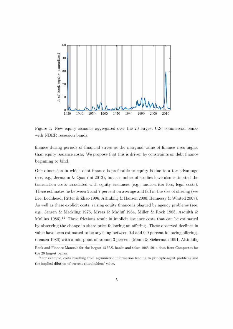
Figure 1: New equity issuance aggregated over the 20 largest U.S. commercial banks
with NBER recession bands.
finance during periods of financial stress as the marginal value of finance rises higher
than equity issuance costs. We propose that this is driven by constraints on debt finance
beginning to bind.
One dimension in which debt finance is preferable to equity is due to a tax advantage
(see, e.g., Jermann & Quadrini 2012), but a number of studies have also estimated the
transaction costs associated with equity issuances (e.g., underwriter fees, legal costs).
These estimates lie between 5 and 7 percent on average and fall in the size of offering (see
Lee, Lochhead, Ritter & Zhao 1996, Altinkilic & Hansen 2000, Hennessy & Whited 2007).
As well as these explicit costs, raising equity finance is plagued by agency problems (see,
e.g., Jensen & Meckling 1976, Myers & Majluf 1984, Miller & Rock 1985, Asquith &
Mullins 1986).12 These frictions result in implicit issuance costs that can be estimated
by observing the change in share price following an offering. These observed declines in
value have been estimated to be anything between 0.4 and 9.9 percent following offerings
(Jensen 1986) with a mid-point of around 3 percent (Mann & Sicherman 1991, Altinkilic
Bank and Finance Manuals for the largest 15 U.S. banks and takes 1965–2014 data from Compustat for
the 20 largest banks.12For example, costs resulting from asymmetric information leading to principle-agent problems and
the implied dilution of current shareholders’ value.
5
& Hansen 2003). Furthermore, whereas the transactional costs fall in the size of issuance,
the implicit costs have been found to rise. Altinkilic & Hansen (2000) find evidence in
support of U-shaped total implicit and explicit issuance fees; the initial decline driven
by falling transactional fees, and the subsequent rise due to the agency frictions. In this
paper, the borrowing constraint is endogenous and equity issuance costs are exogenously
imposed. Following Altinkilic & Hansen (2000), these costs increase in aggregate equity
issuance, acting as a congestion charge. This can be motivated by increases in agency
costs following a large cross-sector equity issuance due, for instance, to costly monitoring
and downward pressure on the issuance price as the market is flooded with new equity.
1.2 Related literature
A starting point for the model is the agency problem proposed in Kiyotaki & Moore
(1997) and extended in the GK banking model. The authors introduce limited contract
enforceability on bank borrowing that results in a financial friction between banks and
households. It is assumed that banks can default on their debts and exit the market, so,
as the courts can only reclaim a proportion of outstanding debts, endogenous borrowing
limits arise. However, unlike other models of financial frictions, such as that of Bernanke,
Gertler & Gilchrist (1999), there is no default in equilibrium, since households will only
loan to a bank that has no incentive to default. This constraint on debt introduces a
wedge between the risk-free rate and the expected discounted return on capital that
fluctuates due to movements in the value of bank assets.
There is a growing literature looking at models with occasionally binding financial con-
straints. For instance, He & Krishnamurthy (2013) propose an occasionally binding
constraint on equity, rather than on debt, in which interest premia rise sharply when
the constraint binds, deepening downturns. The evidence, however, indicates that debt,
rather than equity, is subject to occasionally binding constraints (see, e.g., Kashyap &
Stein 2000, Calomiris & Mason 2003, Ivashina & Scharfstein 2010). In related work,
Brunnermeier & Sannikov (2014) propose a model of constrained equity issuance that
leads to non-linear dynamics; most fluctuations can be absorbed by the intermediaries’
balance sheets but larger negative shocks might lead to unstable, volatile episodes. Ak-
inci & Queralto (2014) and Bocola (2016) present occasionally binding extensions to GK,
the latter to study the pass-through of sovereign risk. In both these papers, whether
6
the constraint is occasionally binding depends crucially on model calibration, unlike our
model. By removing the exogenous bank exit common to these studies, and allowing
them to choose dividend payments, banks will borrow to the edge of the constraint, but
can always raise equity finance for free in the vicinity of the steady state. It follows that
credit crunches are occasional phenomena, in contrast to Akinci & Queralto (2014) and
Bocola (2016), where it is implied that banks are constrained in the steady state. In
related work, Jermann & Quadrini (2012) present a model that differentiates between
the costs of debt and equity finance. This results in countercyclical equity issuance via a
similar mechanism to our model, however, as with GK, the financial constraint is always
binding and not subject to the endogenous variation that our model implies. There
have been models of occasionally constrained household borrowing, including Guerri-
eri & Iacoviello (2017), who show that collateral constraints ceased to bind during the
2001–2006 U.S. housing boom but tightened during the crisis, exacerbating the recession
that followed. Other related works include Dixon & Pourpourides (2016), who look at
occasionally binding cash-in-advance constraints, and Abo-Zaid (2015), who imposes a
collateral constraint on firms to guarantee promised wages to workers.
2 The model
The model features a household and firm sector common to the real business cycle liter-
ature, with the banking sector acting to intermediate funds between these two sectors.
2.1 Households
The representative household maximizes expected lifetime utility:
maxCt+s,Ht+s
Et∞∑s=0
βt+sU (Ct+s, Ht+s, Xt+s)
subject to the budget constraint:
Ct +Bt = WtHt +Rt−1Bt−1 +Dt − Et + Πt − Tt,
where Ct is consumption, Ht is hours worked, Xt is a habit stock, Wt is the wage rate,
and Bt is deposits with the bank that pay interest rate Rt in the following period. Dt and
7
Πt are dividends paid and any other profits, respectively; Et is bank equity purchased;
and Tt represents lump-sum taxes. We assume that households cannot lend directly to
firms, so the intermediation provided by banks is necessary to provide funding to firms.
To achieve co-movement between investment and consumption, we employ the prefer-
ences proposed in Jaimovich & Rebelo (2009), which allow for the control of the short-run
wealth effect on labour supply. In particular, we suppose that the period utility takes
the form:
U (Ct, Ht, Xt) =
[Ct − %H1+ψ
t Xt
]1−σc− 1
1− σc,
where:
Xt = Cγt X1−γt−1 ,
where σc > 0 is the intertemporal elasticity of substitution, % > 0 is the utility weight on
leisure, ψ > 0 controls the elasticity of labour supply, and 0 < γ ≤ 1 controls the wealth
effect. When γ = 0, the preferences are equivalent to those of Greenwood, Hercowitz &
Huffman (1988) (GHH) with no wealth effect on labour supply.13
Household optimization leads to the following Euler equation and labour supply condi-
tion:
1 = βEt[λt+1
λt
]Rt
−UH,tλt
= Wt,
where UH,t is the marginal utility of labour, and λCt is the Lagrange multiplier on the
household budget constraint, i.e., the marginal value of income. λCt is given by:
λCt = UC,t + γµtXt
Ct,
where µt is the Lagrange multiplier on equation (2.1), which is given by:
µt = UX,t + β (1− γ)Et[µt+1
Xt+1
Xt
].
13Jaimovich & Rebelo (2009) preferences benefit from being compatible with balanced growth, unlike
the GHH preferences used in GKQ, which are not.
8
2.2 The banking sector
Banks in the model are owned by households. As a result, they maximize their expected
value, i.e., the expected present discounted value of net dividend payments, Dt−Et. In
treating equity issuance as a negative dividend payment, we are following, for example,
Miller & Rock (1985). However, raising equity financing from households will be costly.
The relationship between banks and households is subject to an agency problem, which
arises due to imperfect contract enforcement; banks are able to declare bankruptcy and
exit with creditors able to reclaim only a proportion of the outstanding debt. This
follows the collateral constraints model of Kiyotaki & Moore (1997), and more closely
the extension to the banking sector by GK. However, whereas GK assume an exoge-
nous bank exit rate that fixes the dividend rate and ensures the borrowing constraint
is always binding, our model relaxes this assumption so that net dividend payments
are endogenous and the borrowing constraint is only occasionally binding. While it is
possible to parameterize the GK model to produce an occasionally binding borrowing
constraint, the range of parameters for which this is true is narrow. Our approach avoids
this problem, as, endogenously, in the steady state the bank will always be just on the
edge of the constraint binding, irrespective of parameters. We also give the derivation
of the borrowing constraint a more careful treatment, based on U.S. bankruptcy law. It
turns out that this necessitates a role for government insurance of the banking sector
against extreme tail events.
Bank j raises debt finance Bjt promising to repay RjtB
jt the following period. A govern-
ment guarantee on these savings mean that banks actually need repay only(Rjt − Gt+1
)Bjt
where Gt+1 is only non-zero in the face of an extreme adverse shock that would otherwise
cause a systemic banking collapse. The government funds this insurance via lump-sum
taxes on households. The bank will pay dividends Djt and raise equity Ejt . While mak-
ing dividend payments is costless, we assume there are administrative costs involved in
issuing equity. To bank j the cost is exogenous and linear in equity issuance, being equal
to κtEjt . However, we model κt as an increasing function of aggregate equity issuance.
This captures congestion externalities such as monitoring. Specifically, we let:
κt := κ
[1− exp
(−ν Et
max 0, Vt
)],
where Vt is the value of the entire banking sector, so Et/Vt is the aggregate rate of
9
equity issuance, and where κ ∈ (0, 1) gives the maximum cost of equity issuance and ν
is a parameter that determines the velocity at which κt converges to κ.
Banks raise debt and equity finance in order to lend to the production sector. The lend-
ing channel is characterized by perfect monitoring and perfect contractual enforcement.
Therefore, banks frictionlessly lend to firms against their future profits, and firms offer
banks fully state-contingent debt, or, equivalently, equity. We denote by Sjt the number
of firm shares held by bank j at t, and we assume that each share delivers a gross return
of RKt per unit. We will normalize the units of these shares such that one share entitles
the owner to the gross return from the ownership of one unit of capital.
The book value of bank j at time t is given by:
V jt ≡
[RKt S
jt−1 − (Rt−1 − Gt)Bj
t−1
] 1
1− κt. (1)
This is the cost that households would have to pay in order to create a “copy” of bank
j. Were equity issuance impossible (i.e., were κt = 1), then creating a “copy” of a
bank with positive net worth would be impossible, or infinitely expensive. We assume
that once equity is in the banking system, it may be transferred between banks without
incurring additional costs. Thus V jt is also the maximum amount that another bank
would be prepared to pay in order to purchase bank j. As such, V jt gives a “cash-out”
value of the bank.
A bank that decides not to exit next period will face the budget constraint:
Djt + Sjt + (Rt−1 − Gt)Bj
t−1 ≤ Bjt + (1− κt)Ejt +RKt S
jt−1. (2)
As previously stated, the objective of bank j is to maximize its expected value. Addi-
tionally, we suppose that where the household is strictly indifferent between dividends
being paid today or in future, the bank has a preference toward paying dividends now.
This may capture agency problems within the bank that lead to an excess focus on short-
term returns, or it may reflect a remote fear of forced nationalization. In particular, the
bank solves:
V jt = max
Bjt ,S
jt ,E
jt ,D
jt
Djt − E
jt + (1− ι)Et
[Λt,t+1V
jt+1
], (3)
subject to the budget constraint (2) and the borrowing constraint, which is still to
be derived, for ι → 0+, where Λt,t+1 ≡ βλCt+1
λCtis the stochastic discount factor of the
10
shareholders and V jt is the value of the bank. The term (1− ι) is superficially similar to
the exogenous bank exit rate in Kiyotaki & Moore (1997) and GK but, since preferences
are under the limit as ι → 0+, its only impact is to capture banks’ arbitrarily weak
preference toward paying dividends sooner rather than later.14 If the (arbitrarily small)
additional discounting is interpreted as an idiosyncratic bank “death” shock, then a
crucial difference between our approach and that of GK is that whereas the owners of
our banks do not gain any value after the “death” shock (e.g., because the bank has
been forcibly nationalized), in GK, dividends are paid only after the bank is hit with
such a shock.
2.3 Bank exit and default
We now consider the default decision and other aspects of off-equilibrium play that are
nonetheless critical for equilibrium outcomes. If bank j fails to repay outstanding debts
in period t, the bank must file for chapter 7 bankruptcy. Following U.S. law (title 11
U.S.C. §548), any remaining assets are seized and sold at market value. If this is enough
to repay Rt−1Bjt−1, any remaining assets are paid to shareholders as a final dividend;
otherwise, the court will examine the previous two years of dividend payments. If, when
a dividend was paid, the value of the bank’s liabilities were greater than the value of its
assets, or the bank had “unreasonably small capital” at that point, then the dividend
would be deemed fraudulent. In this model, we assume that all dividends paid within
this two-year window would be considered fraudulent as at the point of default the bank
was left insolvent.15 Given that a fraudulent payment had been made, the court would
then attempt to recover these dividends plus interest at the risk-free rate. It is assumed
that this is a costly process due, for instance, to costs associated with tracking down
shareholders, and so the court is able to recover only a fraction (1− θ) of the total
amount sought, where θ ∈ (0, 1). If the amount recovered is sufficient to cover Rt−1Bjt−1
then any remaining funds are returned to shareholders; otherwise, the creditors take a
14ι > 0 is required by our numerical strategy, as we take a perturbation approximation around the
deterministic steady state, which would otherwise be indeterminate. Subject to numerical accuracy
limits though, ι may be set arbitrarily small. This is discussed further in section 4.15This is consistent with the legal definition of “unreasonably small capital” according to which pay-
ments would be considered fraudulent if it later transpired the firm was left with insufficient capital to
repay creditors. See Wittstein & Douglas (2014) for further discussion.
11
haircut.
We first consider the bank’s decision in period t whether to exit that same period. First,
note that for the bank to fully meet its liabilities prior to an exit without default would
require households to contribute max0,−V jt , since V j
t includes the costs of equity
issuance. Indeed, since bank j can always sell itself to another bank and receive V jt ,
the bank can always receive V jt by a default-free exit in period t. As a result, it must
always be the case that V jt ≥ V
jt . Alternatively, the bank can decide to exit via default.
Letting τ = 8 (quarters) denote the horizon to which creditors can reclaim assets, then,
the maximum amount that can be recouped from previous dividend payments is:
(1− θ)τ∑i=1
(i∏
k=1
Rt−k
)Djt−i.
Consequently, the value of a bank exiting in period t is:
max
V jt ,− (1− θ)
τ∑i=1
(i∏
k=1
Rt−k
)Djt−i
.
Thus, as V jt ≥ V
jt , the bank will default if and only if:
V jt < − (1− θ)
τ∑i=1
(i∏
k=1
Rt−k
)Djt−i.
If this occurs for bank j on the equilibrium path, then, by symmetry, all banks will
default. So, to prevent a financial collapse, it would be rational for the government to
bail out the banks in this extreme tail situation. In our model, we assume the government
performs the smallest possible bail-out to avoid such a collapse, by choosing Gt such that
the following complementarity condition holds:
min
Gt, Vt + (1− θ)
τ∑i=1
(i∏
k=1
Rt−k
)Dt−i
= 0.
Thus, the government is effectively offering free insurance on firm equity to banks. Al-
though this policy rules out bank default along the equilibrium path, it will lead to
risk being underpriced relative to the efficient benchmark, since banks internalize the
insurance against tail events that the government is providing. However, without artifi-
cial constraints on when banks can default, such insurance is inescapable, as banks are
undertaking risky investments but promising safe returns.
12
We now move on to consider whether in period t a bank might like to plan to default in
period t+ 1. Although the government insurance prevents unplanned default due to tail
shock realizations, this is not sufficient to rule out defaults in which a bank deviates from
the equilibrium path in advance of their eventual default. It is to avoid such planned
defaults that households will restrict their lending to banks, leading to the borrowing
constraint.
At this point, it is important to clarify the order of moves so as to correctly specify
this off-equilibrium play. In particular, we assume that households observe all bank and
aggregate variables from t−1 but only the period t aggregate shocks before choosing the
maximum amount they are prepared to deposit at the bank in period t. The bank then
chooses its individual variables subject to the implied borrowing constraint. The choice
of this ordering is important; if households could observe bank behaviour in advance of
borrowing decisions, then they would not lend to any bank that took an off-equilibrium
action, as this would be interpreted as a preparation for default.
Now, the value of bank j at time t of preparing to default in t+ 1 is given by:
V Xt = Dj
t − Ejt − (1− ι)Et [Λt,t+1] (1− θ)
τ∑i=1
(i∏
k=1
Rt+1−k
)Djt+1−i,
Suppressing the bank indices for neatness, we postulate that the borrowing constraint
takes the form:
Bt ≤ AtVt +τ−1∑i=1
Fi,tDt−i, (4)
for some values independent of the decisions of the bank in question A, F1,t, . . . , Fτ−1,t.
The linearity of the borrowing constraint follows from the linearity of the objective
function and the budget constraint in the state variables. The household will choose the
limit on Bt so that the bank weakly prefers not to deviate from the equilibrium path by
planning to default. Maximizing the value of exit subject to the borrowing constraint
and the budget constraint implies that the borrowing constraint will bind, the bank will
make no further investments (i.e., St = 0), and will issue no equity (i.e., Et = 0). Again,
because the budget constraint, objective function, and borrowing constraint are linear in
the state and choice variables, the bank value function must be homogeneous of degree
one in the state. Furthermore, as the bank can sell and then re-buy assets for the same
13
price, the value function must have a linear representation in Vt and Dt−iτ−1i=1 , so:
Vt =MtVt +τ−1∑i=1
Ni,tDt−i, (5)
for some values independent of the decisions of the bank in question Mt, N1,t, . . . ,
Nτ−1,t.
To prevent default, the household must ensure that Vt ≥ V Xt . The weakest condition
ensuring this implies:
At =Mt
1− (1− ι) (1− θ)− (1− κt) , (6)
Fi,t =Ni,t + (1− ι) (1− θ)
∏ik=1Rt−k
1− (1− ι) (1− θ). (7)
The bank maximizes objective (3) subject to the borrowing constraint (4), the budget
constraint (2), and positivity constraints on Dt and Et, where the value and book value
of the bank are given by equations (5) and (1), respectively. By taking first-order
conditions, substituting these first-order conditions back into the problem’s Lagrangian
and then matching the terms in each state variable, we arrive at:
(1− ι)Et[Λt,t+1
1−κt1−κt+1
Mt+1
Mt(Rt − Gt+1)
]=(
1− λBt(1−κt)(1−(1−ι)(1−θ))
), (8)
Ni,t = Zi,t(1− ι) (1− θ)
1− (1− ι) (1− θ)
i∏k=1
Rt−k, i = 1, · · · , τ − 1, (9)
where:
Zi,t ≡λBt
1− λBtMt
1− κt+ (1− ι)Et [Zi+1,t+1] , i = 1, · · · , τ − 2,
Zτ−1,t ≡λBt
1− λBtMt
1− κt, (10)
and where λBt is the Lagrange multiplier on the borrowing constraint. The first condition
gives the law of motion for the marginal value of the bank book value; the second for
the marginal value of past dividend payments. Defining:
Ht ≡ λBt +Mt
(1− λBt
(1− κt) (1− (1− ι) (1− θ))
), (11)
and:
Ξt,t+1 ≡ (1− ι)Λt,t+11− κt
1− κt+1
Mt+1
Ht,
14
equation (8) and the first-order conditions for dividends, equity and shares can be written
as:
λBt = Ht −HtEt [Ξt,t+1 (Rt − Gt+1)] ≥ 0, (12)
λDt = Ht − (1− ι) (1− κt)Et [Λt,t+1N1,t+1]− (1− κt) ≥ 0, (13)
λEt = 1−Ht ≥ 0, (14)
1 = Et[Ξt,t+1R
Kt+1
], (15)
where λDt and λEt are the Lagrange multipliers on the positivity constraints on dividend
payments and equity issuance, respectively. The final equation implies that Ξt,t+1 is the
pricing kernel (or stochastic discount factor) for firm equity.
2.4 Firms
The final good is produced by a perfectly competitive industry with access to the tech-
nology:
Yt = (AtHt)1−αKt−1
α,
where At is a stationary stochastic process. Firms producing the final good choose the
amount of labour, Ht, and capital, Kt−1, to hire in order to maximize their profits, which
are given by Yt−WtHt−ZtKt−1, where Zt is the rental rate of capital. Hence, from the
first-order conditions, we have the usual marginal product conditions:
Wt = (1− α)YtHt,
Zt = αYtKt−1
.
The capital stock is owned by firms in a perfectly competitive industry with access to the
following technology for producing the next period’s installed capital from investment
and the previous period’s capital:
Kt =
[1− Φ
(ItIt−1
)]It + (1− δ)Kt−1, (16)
where It is investment (of the final good), δ is the depreciation rate and Φ governs the
Christiano, Eichenbaum & Evans (2005) style of investment adjustment costs, where
15
Φ (1) = Φ′ (1) = 0 and Φ′′ (·) = φ > 0. Since these capital-producing firms are owned by
banks, they choose investment to maximize:
Et∞∑s=0
[s−1∏k=0
Ξt+k,t+k+1
](Zt+sKt+s−1 − It+s).
Therefore, from the capital producers’ first-order conditions:
1 = Qt
(1− Φ
(ItIt−1
)− Φ′
(ItIt−1
)ItIt−1
)+ Et
[Ξt,t+1Qt+1Φ′
(It+1
It
)(It+1
It
)2],
1 = Et[Ξt,t+1
Zt+1 + (1− δ)Qt+1
Qt
],
where Qt is the Lagrange multiplier on equation (16), i.e., the value of a unit of installed
capital. From comparing the second equation with equation (15), we see that the gross
rate of return on shares in capital producers must be given by RKt ≡ [Zt + (1− δ)Qt] 1Qt−1
(i.e., the gross return on capital), since all capital producer returns are transferred to
the bank in all states of the world.
Finally, the model is closed with the resource constraint
Yt = Ct + It.
3 Theoretical results
Before turning to numerical results, we will discuss a few key theoretical properties
of the model. All proofs are contained in Appendix A. We begin by focusing on the
Lagrange multipliers and the coefficients of the bank’s value function, as these offer some
immediate insight into the importance of the financial constraints.
Proposition 1 ∀t, λEt = 0: that is, the positivity constraint on equity issuance never
binds.
This result brings computational benefits, as it means we can drop the inequality con-
straint Et ≥ 0, which will speed up simulation. Additionally, this result suggests that it
can be optimal for banks to simultaneously issue equity and make dividend payments,
thanks to the “signalling” value of dividend payments. Note that we are not using “sig-
nalling” in the typical asymmetric information sense here. Rather, the bank’s decision
to pay dividends communicates to households that they are unlikely to default in future,
16
as dividend payments can be partially recovered following default, leading households
to raise the borrowing limit. Without this channel, households would care only about
Dt−Et, and so, since issuing equity is costly, it could never be optimal to pay dividends
while issuing equity.
To understand when simultaneous dividend and equity issuance might occur, recall that:
λDt = κt − (1− ι) (1− κt)Et [Λt,t+1N1,t+1] ≥ 0.
This tells us that if the marginal “signalling” value of paying a dividend is positive
(i.e., if Et [Λt,t+1N1,t+1] > 0), then it must be the case that κt > 0, which in turn
implies that Et > 0, as κt is an increasing function of Et, with κt = 0 when Et = 0.
Furthermore, since issuing equity is costly, the total amount issued will be as low as
possible. Therefore, if the bank has no other reason to issue equity, as the borrowing
constraint is not binding, then it will be the case that λDt = 0, implying that dividends
payments are being funded by equity issuance. Such a situation is not implausible, as
N1,t > 0 if Prt(λBt+k−1 > 0) > 0 for any k ∈ 1, . . . , τ. It follows that there is always
a signalling value of making dividend payments, and as such equity will be issued every
period. That said, if κ′t (Et) is sufficiently high in the region of Et = 0, then the amount
of equity issued will be very low and could disappear entirely were there also fixed costs
of issuance in our model.
Proposition 1 also implies that Ht = 1, and so the stochastic discount factor applied to
firms becomes:
Ξt,t+1 ≡ (1− ι)Λt,t+11− κt
1− κt+1Mt+1. (17)
From this, it is easy to see that if the marginal value of an additional unit of funding
is equal to one, and if the cost of equity issuance is constant, then in the limit as
ι → 0+, equation (17) will equal the household discount factor; that is to say, financial
intermediation would be efficient.
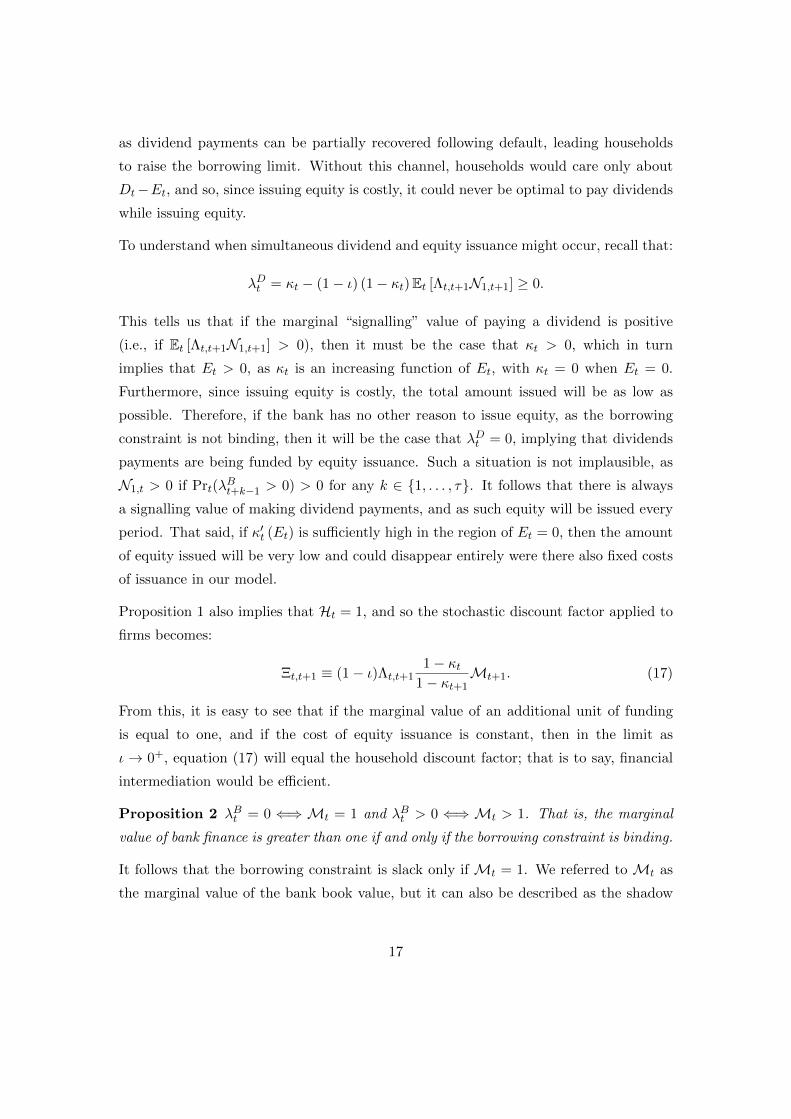
Proposition 2 λBt = 0 ⇐⇒ Mt = 1 and λBt > 0 ⇐⇒ Mt > 1. That is, the marginal
value of bank finance is greater than one if and only if the borrowing constraint is binding.
It follows that the borrowing constraint is slack only if Mt = 1. We referred to Mt as
the marginal value of the bank book value, but it can also be described as the shadow
17
price of bank finance; it is intuitive that this increases above unity as the bank becomes
financially constrained.
The spread between the savings rate and the expected return on equity gives a measure
of the current strength of the financial friction. We are particularly interested in the
component of the spread that emerges from the agency problem, rather than the risk
premium component. This component is captured by the Lagrange multiplier on the
borrowing constraint, λBt . To see this, note that from equations (12) and (15), we have:
λBt = Et[Ξt,t+1
(RKt+1 − (Rt − Gt+1)
)].
The size of the spread depends crucially on the cost of issuing equity; if the cost were
always zero, there would be no financial friction as banks would issue equity until their
borrowing constraint was slack. In the benchmark GK case, equity finance is ruled out
entirely, which sets κt = 1 for all t. (GK also propose an extension in which equity finance
can be issued but is subject to the same type of friction as debt finance.) Our approach
highlights the role that costly equity issuance plays when debt finance is constrained.
The marginal value of bank finance, Mt, is the value of one extra dollar of finance on
the balance sheet of the bank; if the bank can raise finance via reductions in dividend
payment or increased borrowing, then this will equal one dollar. As equity is issued and
κt increases, Mt rises above unity. An additional dollar of finance reduces the need to
raise costly equity by one dollar today, and by lowering the leverage of the bank, will
relax the borrowing constraint in this and future periods.
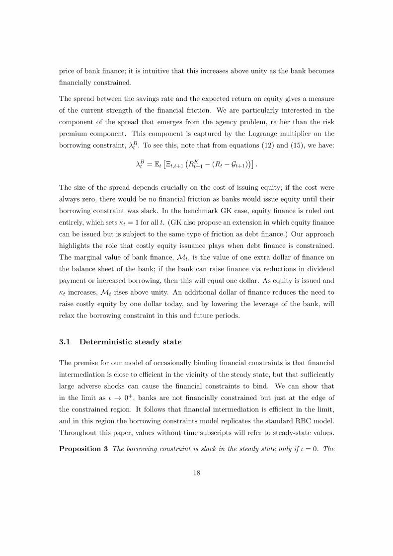
3.1 Deterministic steady state
The premise for our model of occasionally binding financial constraints is that financial
intermediation is close to efficient in the vicinity of the steady state, but that sufficiently
large adverse shocks can cause the financial constraints to bind. We can show that
in the limit as ι → 0+, banks are not financially constrained but just at the edge of
the constrained region. It follows that financial intermediation is efficient in the limit,
and in this region the borrowing constraints model replicates the standard RBC model.
Throughout this paper, values without time subscripts will refer to steady-state values.
Proposition 3 The borrowing constraint is slack in the steady state only if ι = 0. The
18
banking sector is at the edge of the constrained region in the steady state in the limit as
ι→ 0+.
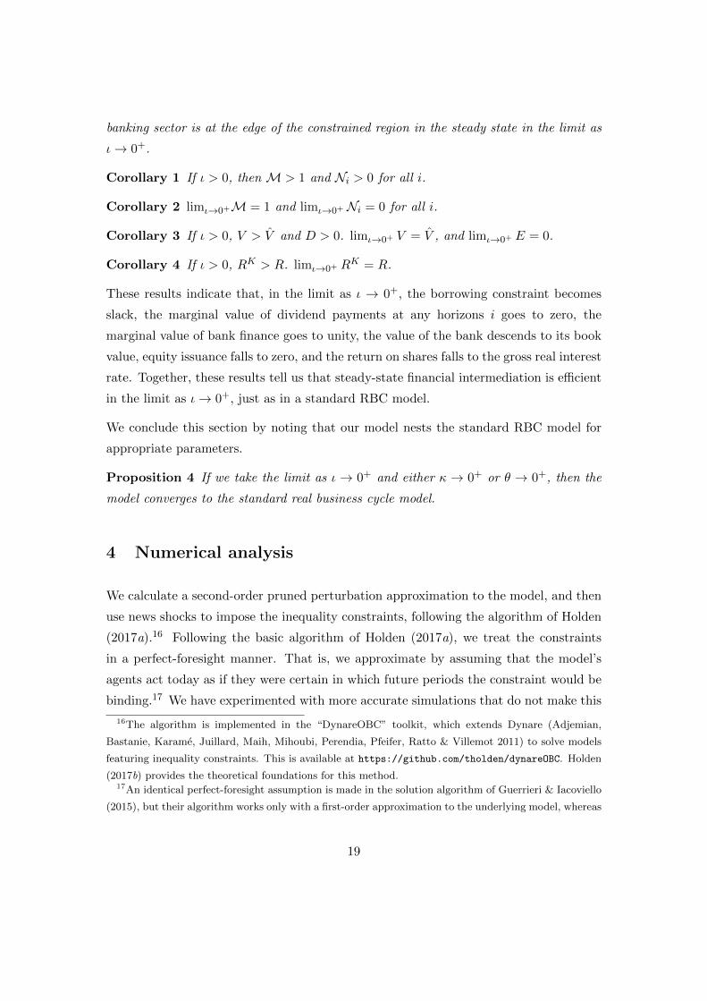
Corollary 1 If ι > 0, then M > 1 and Ni > 0 for all i.
Corollary 2 limι→0+M = 1 and limι→0+ Ni = 0 for all i.
Corollary 3 If ι > 0, V > V and D > 0. limι→0+ V = V , and limι→0+ E = 0.
Corollary 4 If ι > 0, RK > R. limι→0+ RK = R.
These results indicate that, in the limit as ι → 0+, the borrowing constraint becomes
slack, the marginal value of dividend payments at any horizons i goes to zero, the
marginal value of bank finance goes to unity, the value of the bank descends to its book
value, equity issuance falls to zero, and the return on shares falls to the gross real interest
rate. Together, these results tell us that steady-state financial intermediation is efficient
in the limit as ι→ 0+, just as in a standard RBC model.
We conclude this section by noting that our model nests the standard RBC model for
appropriate parameters.
Proposition 4 If we take the limit as ι → 0+ and either κ → 0+ or θ → 0+, then the
model converges to the standard real business cycle model.
4 Numerical analysis
We calculate a second-order pruned perturbation approximation to the model, and then
use news shocks to impose the inequality constraints, following the algorithm of Holden
(2017a).16 Following the basic algorithm of Holden (2017a), we treat the constraints
in a perfect-foresight manner. That is, we approximate by assuming that the model’s
agents act today as if they were certain in which future periods the constraint would be
binding.17 We have experimented with more accurate simulations that do not make this
16The algorithm is implemented in the “DynareOBC” toolkit, which extends Dynare (Adjemian,
Bastanie, Karame, Juillard, Maih, Mihoubi, Perendia, Pfeifer, Ratto & Villemot 2011) to solve models
featuring inequality constraints. This is available at https://github.com/tholden/dynareOBC. Holden
(2017b) provides the theoretical foundations for this method.17An identical perfect-foresight assumption is made in the solution algorithm of Guerrieri & Iacoviello
(2015), but their algorithm works only with a first-order approximation to the underlying model, whereas
19
perfect-foresight approximation, and we found qualitatively similar results, suggesting
that the precautionary effects associated with the bound are not overly important. How-
ever, performing calibration and producing average impulse responses at this higher level
of accuracy are computationally difficult as the constraint is so close to binding in the
steady state. Thus, for consistency we treat the bound in this perfect-foresight manner
throughout. However, since we have a second-order solution to the underlying model, we
will still capture precautionary effects stemming from the model’s other non-linearities.
Because we perturb around the non-stochastic steady state, a strictly positive ι is nec-
essary. To see this, suppose that both in this period and in the next, the borrowing
constraints were slack. Then, a unit increase in dividend payments could be paid for
by a unit increase in deposits now followed by a reduction in dividend payments of Rt
in the next period. Thus, by the household Euler equation, households are indifferent
about the level of dividends in this case.18 Including ι > 0 in the banker’s discounting
resolves this indeterminacy, and pins down the deterministic steady state. In practice,
we set ι := 10−8 to minimize the departure from the ι → 0+ world of our theoretical
results, without introducing numerical problems.
4.1 Model parameters
We compare our numerical results to two benchmarks. A standard RBC model with
Et[Λt,t+1R
Kt+1
]= Et [Λt,t+1]Rt so financial intermediation is efficient, and the GK bor-
rowing constraints model with equity issuance, as outlined in Appendix B. These two
benchmarks provide a never-binding financial friction in the case of the RBC model, and
an always-binding financial friction in the case of the GK model.
Parameters common to the RBC literature are chosen to target a number of long-run
ratios consistent with the literature. A discount factor β = 0.995 is chosen to achieve
an average yearly real interest rate close to 2 percent; capital depreciates at 2.5 percent
per quarter and the capital share is chosen to be α = 0.3 as is standard in the literature.
the algorithm of Holden (2017a) can handle higher-order approximations. The Holden (2017a) algorithm
also allows us to be sure that when there is multiplicity, we are choosing the solution that escapes the
bound as soon as possible.18More generally, households cannot be sure that the bank’s borrowing constraint will be slack next
period, and so they might strictly prefer one unit of dividends today to Rt units next period.
20
We choose % = 2.6 to target a steady state value of hours to equal about one-third.
Following Jaimovich & Rebelo (2009), we choose γ = 0.001, so it is small and positive,
and choose ψ = 0.4, which corresponds to a Frisch elasticity of 2.5 when preferences take
the GHH form. The second derivative of the investment adjustment cost is set as φ = 4
and the (inverse) intertemporal elasticity of substitution is chosen as σc = 2, both within
typical ranges from the literature. For the equity issuance costs, we choose a value for
κ of 10 percent and set ν = 400, which, in a fully non-linear solution, would imply that
the costs would converge to the maximum for very small issuances. In our numerical
simulations, the issuance costs typically fall in the 3 to 8 percent range.
The standard deviation of the total factor productivity shock, σa = 0.0061, is calibrated
to hit a standard deviation of output of 1.015 percent,19 and the persistence ρa = 0.95 is
chosen to target a first-order output autocorrelation of 0.86.20 We choose the proportion
of assets that are unrecoverable after default, θ = 0.67, to target a standard deviation of
the spread between the deposit rate and the risky return on capital of 0.18 percentage
points quarterly.21 As the spread is close to zero in the unconstrained economy, the
volatility of the spread is a natural choice for an additional target; in the absence of
features such as liquidity premia, differing tax treatments and true default risk, the
model inevitably underpredicts the mean spread.22
19This requires σa = 0.0061 in the RBC model and 0.0057 in the GK model.20Non-banking data is 1983Q3–2016Q3 U.S. time series from https://fred.stlouisfed.org: GDP,
FPI and PCEC for output, investment and consumption respectively, deflated using GDPDEF with
CNP160V to convert to per capita. The Hodrick-Prescott filter is applied to these time series. The
spread is that between Moody’s Seasoned BAA and AAA Corporate Bond yields. New equity issuance
is as described in Baron (2017) for the largest 20 U.S. commercial banks. For dividend payments, we
sum dividends and share repurchases from Baron’s (2017) data.21θ is calibrated to 0.89 in the GK model with the same target.22In the GK model, there are two additional parameters that control the survival rate of bankers and
the amount transferred to new bankers, as well as parameters controlling outside equity issuance. The
banker survival rate is equivalent to a dividend rate but has to be set high to ensure an always-binding
constraint. We follow GK and set this to 0.975, which is equivalent to an expected survival rate of 10
years, and set the proportion of bank equity transferred to the new “start-ups” equal to 0.3. These allow
a mean spread approximately equal to the observed 0.57 percentage points and a bank leverage ratio
close to the average of 4, targeted in GK. We follow GKQ with our choice of equity issuance parameter
values.
21
4.2 Impulse response functions and simulations
In order to assess the propagation of shocks and the role of the financial constraints, we
compute the median impulse response functions for shocks to productivity and capital
quality.23 This follows GK, who argue that negative capital quality shocks should not be
considered physical depreciation of capital, but rather represent some form of economic
obsolescence; they also suggest a possible micro-foundation. As in GK, the inclusion of
the capital quality shocks allows for the characterization of occasional “disaster” shocks.
In particular, we will examine the impacts of a 5 percent unanticipated decline in capital
quality.
Let us consider the role of the borrowing constraint following such a disturbance. When
either the banks’ demand for funding increases, or the borrowing constraint tightens due
to a relative decline in the banks’ continuation value, the banks must raise equity finance.
If the bank is unable to raise sufficient finance through retained earnings, they must sell
equity, paying issuance costs that rise in the volume of issuance. This causes the expected
marginal value of bank finance, Mt+1, to increase above unity. As dividend payments
relax the borrowing constraint, it is optimal for the bank to keep paying dividends even
as they begin to issue equity. Indeed, past dividends become particularly important to
the bank once financially constrained; the lower the past dividend payments, the tighter
the borrowing constraint. This is also true for the interest rate; the lower the interest
rate over the previous two years, the tighter the constraint.
Now, recall that the households discount using the stochastic discount factor Λt,t+1,
whereas equity is priced using Ξt,t+1. The latter augments the former with the marginal
value of bank finance, implying that in the unconstrained case, Λt,t+1 = Ξt,t+1, while
Λt,t+1 < Ξt,t+1 when there is a positive probability of financial constraints binding. The
augmented stochastic discount factor is asymmetric asMt ≥ 1, and has higher volatility
than the household stochastic discount factor; if the expected marginal utility of future
consumption increases relative to that of current consumption, as would be expected
following an adverse shock, then Λt,t+1 would increase. Because the expected value of
Mt,t+1 is also likely to rise, Ξt,t+1 rises further still. This introduces a hedging value of
debt finance that increases as the financial constraint tightens. Because of this, when a
23We take the median of the difference between 256 pairs of simulation runs, where each pair of runs
has identical shocks, apart from one additional impulse in period 100 for the first of each pair.
22
0 20 40
-3
-2
-1Y
0 20 40
-4
-2
0I
0 20 40
-2
-1.5
-1H
0 20 40
0
0.2
0.4
∆
0 20 40
0
0.05
0.1
0
1
2D/N
0 20 40
-0.1
0
0.1
-5
0
5E/N
Our Model RBC GK
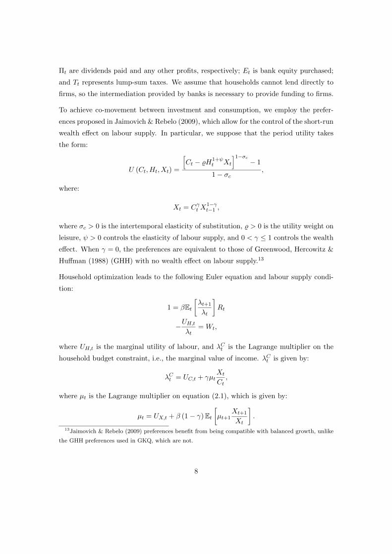
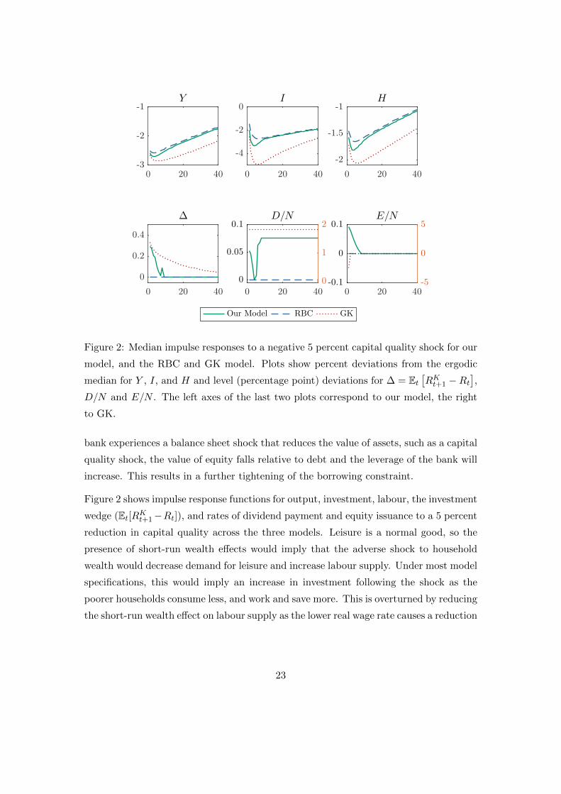
Figure 2: Median impulse responses to a negative 5 percent capital quality shock for our
model, and the RBC and GK model. Plots show percent deviations from the ergodic
median for Y , I, and H and level (percentage point) deviations for ∆ = Et[RKt+1 −Rt
],
D/N and E/N . The left axes of the last two plots correspond to our model, the right
to GK.
bank experiences a balance sheet shock that reduces the value of assets, such as a capital
quality shock, the value of equity falls relative to debt and the leverage of the bank will
increase. This results in a further tightening of the borrowing constraint.
Figure 2 shows impulse response functions for output, investment, labour, the investment
wedge (Et[RKt+1−Rt]), and rates of dividend payment and equity issuance to a 5 percent
reduction in capital quality across the three models. Leisure is a normal good, so the
presence of short-run wealth effects would imply that the adverse shock to household
wealth would decrease demand for leisure and increase labour supply. Under most model
specifications, this would imply an increase in investment following the shock as the
poorer households consume less, and work and save more. This is overturned by reducing
the short-run wealth effect on labour supply as the lower real wage rate causes a reduction
23
in labour supply.24 Banks in GK are always financially constrained but following the
capital quality shock, the financial constraint tightens further, causing a larger decline
in investment relative to the RBC model. Bank leverage increases when the value of
assets falls, causing a reduction in both the borrowing limit and equity issuance. The
contraction in available funds leads to a deeper decline in investment that remains below
the RBC model into the long run. The effective dividend rate is fixed by the constant
probability of banker exit. The decline in investment in our model is close to that
of the GK model on impact, but begins to converge back to the RBC model after
about five quarters. Nonetheless, the episode of constrained finance is persistent, with
the investment wedge taking around three years to return to normal levels. Unlike in
GK, banks increase equity issuance when the borrowing constraint tightens, and, due
to the signalling role of dividend payments in relaxing the borrowing constraint, it is
unnecessary for payments to cease before banks begin to issue equity. Indeed, for several
periods, the banks simultaneously pay dividends and issue equity. Due to the costs of
equity issuance, the marginal bank funding cost increases above the savings rate; this is
the force behind the sharp rise in the interest spread and the deeper fall in investment
relative to the RBC model.
A final point to note is that the impulse response functions are asymmetric and non-
monotonic; the financial accelerator effects decline significantly as the size of adverse
shocks falls, and are all but absent for shocks of the opposite sign. We illustrate this
with further impulse responses in Appendix C.
4.2.1 Simulated moments
Table 1 reports simulated moments and cross-correlations for the three models together
with those computed from the data. Our model introduces significant skewness in the
interest spread that is entirely missing from the GK models, as well as skewness in equity
issuance that arises due to occasional episodes of sharp issuances. Furthermore, when
24Investment does fall in both GK and our model on impact with standard King-Plosser-Rebelo (KPR)
preferences as financial constraints tighten, but quickly rebounds, leading to an investment boom. The
increase in investment can also be overturned with habits in consumption (see, e.g., Cochrane & Campbell
1999) as the substitution between consumption and savings become costly. We choose the Jaimovich-
Rebelo approximation to GHH preferences, as both habits in consumption and KPR preferences imply
a counterfactual increase in labour.
24
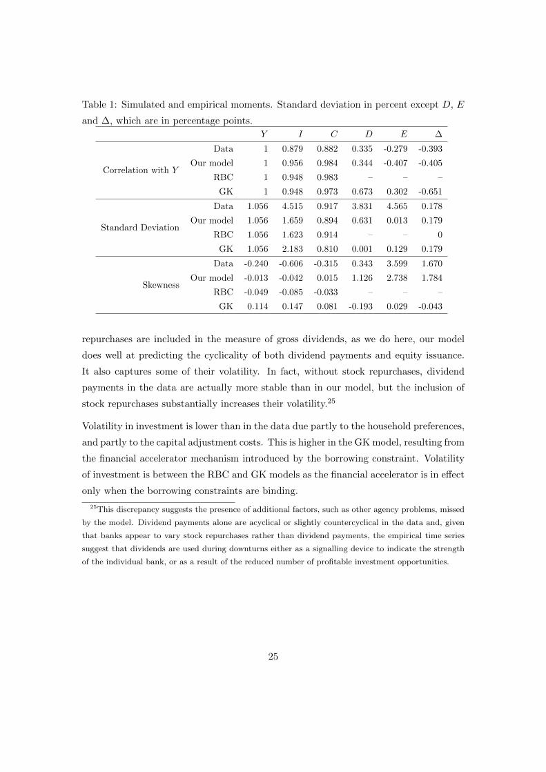
Table 1: Simulated and empirical moments. Standard deviation in percent except D, E
and ∆, which are in percentage points.
Y I C D E ∆
Correlation with Y
Data 1 0.879 0.882 0.335 -0.279 -0.393
Our model 1 0.956 0.984 0.344 -0.407 -0.405
RBC 1 0.948 0.983 – – –
GK 1 0.948 0.973 0.673 0.302 -0.651
Standard Deviation
Data 1.056 4.515 0.917 3.831 4.565 0.178
Our model 1.056 1.659 0.894 0.631 0.013 0.179
RBC 1.056 1.623 0.914 – – 0
GK 1.056 2.183 0.810 0.001 0.129 0.179
Skewness
Data -0.240 -0.606 -0.315 0.343 3.599 1.670
Our model -0.013 -0.042 0.015 1.126 2.738 1.784
RBC -0.049 -0.085 -0.033 – – –
GK 0.114 0.147 0.081 -0.193 0.029 -0.043
repurchases are included in the measure of gross dividends, as we do here, our model
does well at predicting the cyclicality of both dividend payments and equity issuance.
It also captures some of their volatility. In fact, without stock repurchases, dividend
payments in the data are actually more stable than in our model, but the inclusion of
stock repurchases substantially increases their volatility.25
Volatility in investment is lower than in the data due partly to the household preferences,
and partly to the capital adjustment costs. This is higher in the GK model, resulting from
the financial accelerator mechanism introduced by the borrowing constraint. Volatility
of investment is between the RBC and GK models as the financial accelerator is in effect
only when the borrowing constraints are binding.
25This discrepancy suggests the presence of additional factors, such as other agency problems, missed
by the model. Dividend payments alone are acyclical or slightly countercyclical in the data and, given
that banks appear to vary stock repurchases rather than dividend payments, the empirical time series
suggest that dividends are used during downturns either as a signalling device to indicate the strength
of the individual bank, or as a result of the reduced number of profitable investment opportunities.
25
5 Conclusion
This paper embeds a model of banking into a real business cycle framework, resulting
in a model that generates occasional endogenous credit crunches. In the vicinity of
the deterministic steady state, the model behaves much like a standard RBC model:
financial intermediation is efficient and the interest rate spread is equal to the standard
risk premium. Credit crunches are precipitated by sufficiently large adverse shocks that
cause the bank financing constraint to bind. This is the result of an increased incentive
for banks to divert funds and declare bankruptcy caused by a reduction in expected
bank profits. Banks are able to issue equity when debt finance is constrained, but
issuance costs introduce a wedge between the risk-free rate and the risky return to
capital, resulting in reduced investment and output.
By removing the exogenous bank exit rate common to many similar models and allowing
endogenous dividend payments, we find that the borrowing constraint is always occa-
sionally binding, independent of calibration. Furthermore, in our model, credit crunches
are truly an occasional phenomena in contrast to the majority of existing models in
which financial constraints bind in steady state. A key contribution is a careful treat-
ment of the Kiyotaki & Moore (1997) agency problem extended in GK. By modelling
the U.S. law relating to bankruptcy, we reveal a potentially important signalling role for
dividends in acting to relax the borrowing constraint. Finally, our model gives a number
of improvements in the empirical fit of simulated time series. Notably, we capture the
strong positive skewness in the interest spread and equity issuance that are missing in
the standard RBC and GK models. We also replicate the countercyclical equity issuance
observed in the data, contrary to other papers, such as GKQ, which predict procyclical
equity issuance.
26
References
Abo-Zaid, S. (2015), ‘Optimal long-run inflation with occasionally binding financial con-
straints’, European Economic Review 75, 18–42.
Adjemian, S., Bastanie, H., Karame, F., Juillard, M., Maih, J., Mihoubi, F., Perendia,
G., Pfeifer, J., Ratto, M. & Villemot, S. (2011), ‘Dynare : Reference Manual Version
4’, Dynare Working Paper Series (1), 160.
Akinci, O. & Queralto, A. (2014), Banks, Capital Flows and Financial Crises, Number
1121, Board of Governors of the Federal Reserve System, International Finance
Discussion Papers.
Altinkilic, O. & Hansen, R. S. (2000), ‘Are there economies of scale in underwriting fees?
Evidence of rising external financing costs’, Review of Financial Studies 13(1), 191–
218.
Altinkilic, O. & Hansen, R. S. (2003), ‘Discounting and underpricing in seasoned equity
offers’, Journal of Financial Economics 69(2), 285–323.
Asquith, P. & Mullins, D. W. (1986), ‘Equity issues and offering dilution’, Journal of
Financial Economics 15(1-2), 61–89.
Babihuga, R. & Spaltro, M. (2014), Bank Funding Costs for International Banks, Work-
ing paper, International Monetary Fund, Washington D.C.
Baron, M. D. (2017), Countercyclical bank equity issuance.
Bernanke, B. S., Gertler, M. & Gilchrist, S. (1999), The Financial Accelerator in a Quan-
titative Business Cycle Framework, in J. B. Taylor & M. Woodford, eds, ‘Handbook
of Macroeconomics’, Vol. 1, Elsevier B.V., chapter 21, pp. 1341–1393.
Bocola, L. (2016), ‘The Pass-Through of Sovereign Risk’, Journal of Political Economy
124(4), 879–926.
Brunnermeier, M. & Sannikov, Y. (2014), ‘A Macroeconomic Model with a Financial
Sector’, American Economic Review 104(2), 379–421.
Calomiris, C. W. & Mason, J. R. (2003), ‘Consequences of Bank Distress During the
Great Depression’, American Economic Review 93(3), 937–947.
27
Chari, V. V., Kehoe, P. J. & McGrattan, E. R. (2007), ‘Business cycle accounting’,
Econometrica 75(3), 781–836.
Christiano, L. J., Eichenbaum, M. & Evans, C. L. (2005), ‘Nominal rigidities and
the dynamic effects of a shock to monetary policy’, Journal of Political Economy
113(1), 1–45.
Cochrane, J. H. & Campbell, J. Y. (1999), ‘By force of habit: A consumption-based
explanation of aggregate stock market behaviour’, Journal of Political Economy
107(2), 205.
Del Negro, M., Hasegawa, R. B. & Schorfheide, F. (2016), ‘Dynamic prediction pools: An
investigation of financial frictions and forecasting performance’, Journal of Econo-
metrics 192(2), 391–405.
Dixon, H. & Pourpourides, P. M. (2016), ‘On imperfect competition with occasionally
binding cash-in-advance constraints’, Journal of Macroeconomics 50, 72–85.
Fama, E. F. & French, K. R. (2005), ‘Financing decisions: who issues stock?’, Journal
of Financial Economics 76, 549–582.
Gertler, M. & Kiyotaki, N. (2010), ‘Financial intermediation and credit policy in business
cycle analysis’, Handbook of Monetary Economics 3(11), 547–599.
Gertler, M., Kiyotaki, N. & Queralto, A. (2012), ‘Financial crises, bank risk exposure and
government financial policy’, Journal of Monetary Economics 59(SUPPL.), S17–
S34.
Greenwood, J., Hercowitz, Z. & Huffman, G. (1988), ‘Investment, capacity utilization
and the real business cycle’, American Economic Review 78(3), 402–417.
Guerrieri, L. & Iacoviello, M. (2015), ‘OccBin: A toolkit for solving dynamic models with
occasionally binding constraints easily’, Journal of Monetary Economics 70, 22–38.
Guerrieri, L. & Iacoviello, M. (2017), ‘Collateral Constraints and Macroeconomic Asym-
metries’, Journal of Monetary Economics 90, 28–49.
Hall, R. E. (2010), ‘Why does the economy fall to pieces after a financial crisis?’, The
Journal of Economic Perspectives 24(4), 3–20.
28
He, Z. & Krishnamurthy, A. (2013), ‘Intermediary asset pricing’, American Economic
Review 103(2), 732—-770.
Hennessy, C. & Whited, T. M. (2007), ‘How costly is external financing? Evidence from
a structural estimation’, Journal of Finance 62(4), 1705–1745.
Holden, T. (2017a), Computation of solutions to dynamic models with occasionally
binding constraints, Econstor preprints 144569, ZBW - German National Library
of Economics.
Holden, T. (2017b), Existence, uniqueness and computation of solutions to dynamic
models with occasionally binding constraints., Econstor preprints 144570, ZBW -
German National Library of Economics.
Ivashina, V. & Scharfstein, D. (2010), ‘Bank lending during the financial crisis of 2008’,
Journal of Financial Economics 97(3), 319–338.
Jagannathan, M., Stephens, C. P. & Weisbach, M. S. (2000), ‘Financial flexibility and the
choice between dividends and stock repurchases’, Journal of Financial Economics
57(3), 355–384.
Jaimovich, N. & Rebelo, S. (2009), ‘Can news about the future drive the business cycle?’,
American Economic Review 99(4), 1097–1118.
Jensen, C. & Meckling, H. (1976), ‘Theory of the firm: managerial behavior, agency
costs and ownership structure’, Journal of Financial Economics 3, 305–360.
Jensen, M. C. (1986), ‘Agency costs of free cash flow, corporate finance, and takeovers’,
American Economic Review Papers and Proceedings 76(2), 323–329.
Jermann, U. & Quadrini, V. (2012), ‘Macroeconomic Effects of Financial Shocks’, Amer-
ican Economic Review 102(1), 238–271.
Kashyap, A. K. & Stein, J. C. (2000), ‘What do a million observations on banks say about
the transmission of monetary policy?’, American Economic Review 90(3), 407–428.
Kiyotaki, N. & Moore, J. (1997), ‘Credit Cycles’, Journal of Political Economy
105(2), 211–248.
Lee, I., Lochhead, S., Ritter, J. R. & Zhao, Q. (1996), ‘The costs of raising capital’,
Journal of Financial Research 19(1), 59–74.
29
Loderer, C. F. & Mauer, D. C. (1992), ‘Corporate dividends and seasoned equity issues:
An empirical investigation’, The Journal of Finance 47(1), 201–225.
Mankiw, N. G. (2000), ‘The savers-spenders theory of fiscal policy’, American Economic
Review 90(2), 120–125.
Mann, S. V. & Sicherman, N. W. (1991), ‘The agency costs of free cash flow: Acquisition
activity and equity issues’, Journal of Business 64(2), 213–227.
Miller, M. H. & Rock, K. (1985), ‘Dividend policy under asymmetric information’, The
Journal of Finance 40(4), 1031–1051.
Myers, S. C. (1984), ‘The capital structure puzzle’, The Journal of Finance 39(3), 574–
592.
Myers, S. C. & Majluf, N. S. (1984), ‘Corporate financing and investment decisions when
firms have information that investors do not have’, Journal of Financial Economics
13(2), 187–221.
Shin, H. S. (2009), ‘Reflections on Northern Rock: The bank run that heralded the
global financial crisis’, Journal of Economic Perspectives 23(1), 101–119.
Wittstein, J. R. & Douglas, M. G. (2014), ‘In search of the meaning of “unreason-
ably small capital” in constructively fraudulent transfer avoidance litigation’,
Jones Day Publications . http://www.jonesday.com/in-search-of-the-meaning-
of-unreasonably-small-capital-in-constructively-fraudulent-transfer-avoidance-
litigation-12-02-2014/.
30
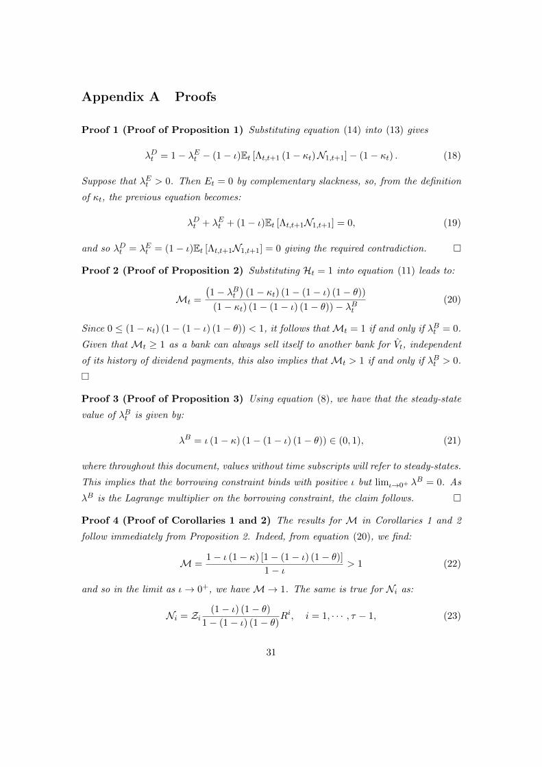
Appendix A Proofs
Proof 1 (Proof of Proposition 1) Substituting equation (14) into (13) gives
λDt = 1− λEt − (1− ι)Et [Λt,t+1 (1− κt)N1,t+1]− (1− κt) . (18)
Suppose that λEt > 0. Then Et = 0 by complementary slackness, so, from the definition
of κt, the previous equation becomes:
λDt + λEt + (1− ι)Et [Λt,t+1N1,t+1] = 0, (19)
and so λDt = λEt = (1− ι)Et [Λt,t+1N1,t+1] = 0 giving the required contradiction.
Proof 2 (Proof of Proposition 2) Substituting Ht = 1 into equation (11) leads to:
Mt =
(1− λBt
)(1− κt) (1− (1− ι) (1− θ))
(1− κt) (1− (1− ι) (1− θ))− λBt(20)
Since 0 ≤ (1− κt) (1− (1− ι) (1− θ)) < 1, it follows that Mt = 1 if and only if λBt = 0.
Given that Mt ≥ 1 as a bank can always sell itself to another bank for Vt, independent
of its history of dividend payments, this also implies that Mt > 1 if and only if λBt > 0.
Proof 3 (Proof of Proposition 3) Using equation (8), we have that the steady-state
value of λBt is given by:
λB = ι (1− κ) (1− (1− ι) (1− θ)) ∈ (0, 1), (21)
where throughout this document, values without time subscripts will refer to steady-states.
This implies that the borrowing constraint binds with positive ι but limι→0+ λB = 0. As
λB is the Lagrange multiplier on the borrowing constraint, the claim follows.
Proof 4 (Proof of Corollaries 1 and 2) The results for M in Corollaries 1 and 2
follow immediately from Proposition 2. Indeed, from equation (20), we find:
M =1− ι (1− κ) [1− (1− ι) (1− θ)]
1− ι> 1 (22)
and so in the limit as ι→ 0+, we have M→ 1. The same is true for Ni as:
Ni = Zi(1− ι) (1− θ)
1− (1− ι) (1− θ)Ri, i = 1, · · · , τ − 1, (23)
31

where:
Zi ≡1− (1− ι)τ−i
ι
λB
1− λBM
1− κ> 0, i = 1, · · · , τ − 1. (24)
So Ni > 0 for i = 1, · · · , τ − 1, but as ι→ 0, Zi → 0 and Ni → 0.
Proof 5 (Proof of Corollary 3) The value of the bank is given by:
V =MV +
τ−1∑i=1
NiD. (25)
Hence, the value of a bank is always greater than its book value for ι > 0, but limι→0+ V =
V .
Now, banks must pay dividends in steady state, at least with ι > 0, for, suppose they
did not. Then, their steady-state value would be zero, by the definition of bank value,
and so since book value is always weakly below value, their steady-state book value would
be non-positive. However, since equity issuance is always strictly positive with ι > 0,
steady-state book-value would be infinite without dividend payments, giving the required
contradiction. Consequently:
λD = κ− (1− ι) βΠ∗N1 (1− κ) = 0, (26)
so:
κ =(1− ι) β
Π∗N1
1 + (1− ι) βΠ∗N1
> 0. (27)
It follows from limι→0+ N1 = 0, that limι→0+ κ = 0 and so there is no equity issuance in
the limit.
Proof 6 (Proof of Corollary 4) Note:
R = (1− ι (1− κ) [1− (1− ι) (1− θ)])RK , (28)
so RK > R but limι→0+ RK = R.
Proof 7 (Proof of Proposition 4) First suppose that κ = 0. In this case, the first
order condition with respect to dividend payments becomes:
λDt = −(1− ι)Et [Λt,t+1N1,t+1] . (29)
32

Now, it follows from the definition of N1,t in equations (9) to (10), that N1,t ≥ 0 for all
t, since λBt ∈ [0, 1], by equation (12). Hence, since λDt ≥ 0, equation (29) in fact implies
that λDt = N1,t = 0 for all t. Consequently, again by equations (9) to (10), we must also
have that λBt = 0 for all t, which in turn implies that Mt = 1 for all t, by Proposition
2. Using this in the definitions of the pricing kernels for bank and firm equity, we find
that when ι = 0 as well, Λt,t+1 = Ξt,t+1 for all t, so financial intermediation is efficient.
The bank is never financially constrained as they can always raise equity finance at no
cost.
Next, suppose that θ = 0. Recall the borrowing constraint is of the form:
Bt ≤ AVt + F1,tDt−1 + · · ·+ Fτ−1,tDt−τ+1. (30)
If θ = 0, then as ι→ 0, it follows from the solutions of the coefficients in equations (6)
and (7), that At → ∞ and Fi,t → ∞ for i = 1, ..., τ − 1. So in the limit as ι → 0,
borrowing becomes unlimited. As in the previous case, it follows that for all t, λBt = 0,
Mt = 1 and Λt,t+1 = Ξt,t+1 if ι = 0, and so financial intermediation is efficient.
Appendix B Gertler & Kiyotaki (2010) model
We describe a version of the GK model extension with equity issuance. The household
and firm sectors are identical to our model, the difference is on the intermediation of
funds between these two sectors. Every period, banks face a constant probability, 1−σB,
of exiting and paying the household a dividend. No dividend is paid if the bank continues,
the bank decides on debt and outside equity finance and issues loans to non-financial
firms. When a bank exits, a new bank takes is place and is transferred a fraction ξB
of the exiting banks’ net worth. Bank activity is subject to financial constraints as the
inside shareholders can divert assets. In particular bank j solves
V jt = max
St,Bt,Et
Et (1− σB)N jt+1 + σBΛt,t+1V
jt+1
s.t. V jt ≥ Θ
(xjt
)Sjt
N jt = RKt S
jt−1 −R
Et Q
Et−1E
jt−1 −Rt−1B
jt−1
Sjt = Bjt +QEt E
jt +N j
t
33
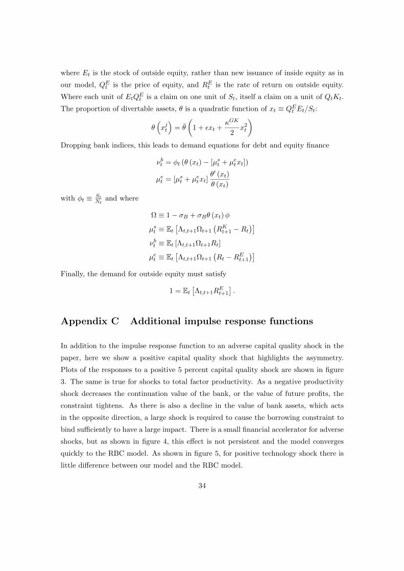
where Et is the stock of outside equity, rather than new issuance of inside equity as in
our model, QEt is the price of equity, and REt is the rate of return on outside equity.
Where each unit of EtQEt is a claim on one unit of St, itself a claim on a unit of QtKt.
The proportion of divertable assets, θ is a quadratic function of xt ≡ QEt Et/St:
θ(xjt
)= θ
(1 + εxt +
κGK
2x2t
)Dropping bank indices, this leads to demand equations for debt and equity finance
νbt = φt (θ (xt)− [µst + µetxt])
µet = [µst + µetxt]θ′ (xt)
θ (xt)
with φt ≡ StNt
and where
Ω ≡ 1− σB + σBθ (xt)φ
µst ≡ Et[Λt,t+1Ωt+1
(RKt+1 −Rt
)]νbt ≡ Et [Λt,t+1Ωt+1Rt]
µet ≡ Et[Λt,t+1Ωt+1
(Rt −REt+1
)]Finally, the demand for outside equity must satisfy
1 = Et[Λt,t+1R
Et+1
].
Appendix C Additional impulse response functions
In addition to the impulse response function to an adverse capital quality shock in the
paper, here we show a positive capital quality shock that highlights the asymmetry.
Plots of the responses to a positive 5 percent capital quality shock are shown in figure
3. The same is true for shocks to total factor productivity. As a negative productivity
shock decreases the continuation value of the bank, or the value of future profits, the
constraint tightens. As there is also a decline in the value of bank assets, which acts
in the opposite direction, a large shock is required to cause the borrowing constraint to
bind sufficiently to have a large impact. There is a small financial accelerator for adverse
shocks, but as shown in figure 4, this effect is not persistent and the model converges
quickly to the RBC model. As shown in figure 5, for positive technology shock there is
little difference between our model and the RBC model.
34
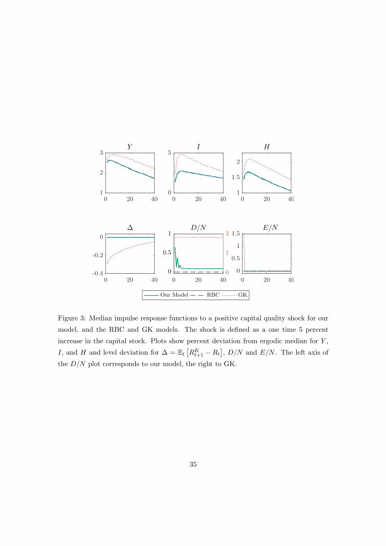
0 20 40
1
2
3Y
0 20 40
0
5I
0 20 40
1
1.5
2
H
0 20 40
-0.4
-0.2
0
∆
0 20 40
0
0.5
1
0
1
2D/N
0 20 40
0
0.5
1
1.5E/N
Our Model RBC GK
Figure 3: Median impulse response functions to a positive capital quality shock for our
model, and the RBC and GK models. The shock is defined as a one time 5 percent
increase in the capital stock. Plots show percent deviation from ergodic median for Y ,
I, and H and level deviation for ∆ = Et[RKt+1 −Rt
], D/N and E/N . The left axis of
the D/N plot corresponds to our model, the right to GK.
35
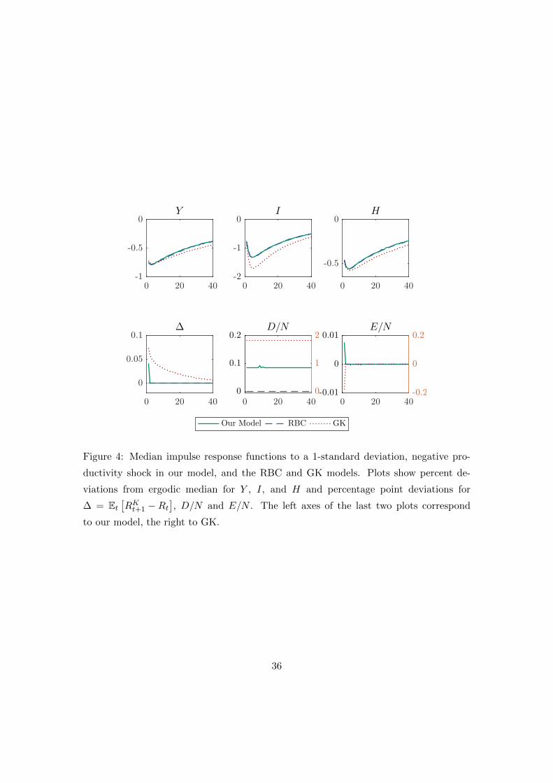
0 20 40
-1
-0.5
0Y
0 20 40
-2
-1
0I
0 20 40
-0.5
0H
0 20 40
0
0.05
0.1∆
0 20 40
0
0.1
0.2
0
1
2D/N
0 20 40
-0.01
0
0.01
-0.2
0
0.2E/N
Our Model RBC GK
Figure 4: Median impulse response functions to a 1-standard deviation, negative pro-
ductivity shock in our model, and the RBC and GK models. Plots show percent de-
viations from ergodic median for Y , I, and H and percentage point deviations for
∆ = Et[RKt+1 −Rt
], D/N and E/N . The left axes of the last two plots correspond
to our model, the right to GK.
36
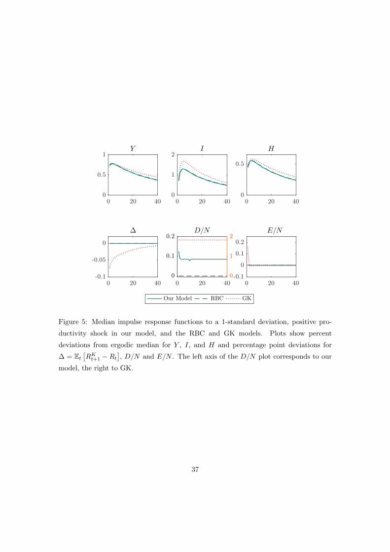
0 20 40
0
0.5
1Y
0 20 40
0
1
2I
0 20 40
0
0.5
H
0 20 40
-0.1
-0.05
0
∆
0 20 40
0
0.1
0.2
0
1
2D/N
0 20 40
-0.1
0
0.1
0.2
E/N
Our Model RBC GK
Figure 5: Median impulse response functions to a 1-standard deviation, positive pro-
ductivity shock in our model, and the RBC and GK models. Plots show percent
deviations from ergodic median for Y , I, and H and percentage point deviations for
∆ = Et[RKt+1 −Rt
], D/N and E/N . The left axis of the D/N plot corresponds to our
model, the right to GK.
37