credit default models

Credit Default Models

Swati [email protected]

Professional Risk Managers’ International Association

May 4, 2016

Mital, Swati (PRMIA) Credit Default Models May 4, 2016 1 / 31

mailto:[email protected]

Credit Risk

What is Credit Risk?

Credit Risk is the risk that the value of the portfolio changes due tochanges in the credit quality of the ”obligors” due to defaults or ratingdowngrade.Products: Loans, Sovereign Bonds, Corporate Bonds and CreditDerivatives. Ignore Equity. We focus on corporate credit models not retailscoring models.

Why model Credit Risk?

Measure Risk in porfolio of credit risky instruments

Compute Regulatory Capital

Compute Economic Capital

Perform Risk Adjusted comparison of different porfolios


Agenda

Focus on, broadly speaking, four types of Credit Default Models

Merton’s Structural Model

Extension to Merton’s Model (KMV Model)

Ratings based Model

Multivariate Factor Models

We also have a brief section on

Reduced Form Model (Bernoulli Mixture Model)

Finally, we cover Copulas and how they are used for Default Modelling

Default Modelling with Copulas


Notations

Let the time interval be fixed [0,T ]. Let τi be time to default for obligor i .Let Yi = 1τi≤T be the default indicator.

Then, we can represent the probability of default for obligor i as,

PDi = P(Yi = 1) = 1− P(Yi = 0) = P(τi ≤ T ) (1)

Let EADi be the exposure at default and LGDi be the loss given default.Then the default loss on a porfolio is,

Default Loss =n∑

i=1

EADi × Yi × LGDi (2)

Since Yi is a Bernoulli r.v., E[Yi ] = PDi . This gives us the Expected valueof the default loss. However, we are interested in different quantiles of theloss distribution function.


Structural Models

In 1974, Merton showed how the Black Scholes Option Pricing theory canbe used to estimate a firm’s probability of default and credit spreads.

Assumptions in Merton’s structural Credit Risk Model:

Firm value, Vt , is financed by equity, St , and, debt, Bt

Vt = St + Bt , 0 ≤ t ≤ T (3)

Debt is a single zero coupon bond with face value B and time tomaturity T

Default occurs when the value of the firm, VT , goes below theoutstanding debt, B. This can be determined from the firm’s balancesheet.


Structural Models

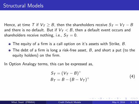
Hence, at time T if VT ≥ B, then the shareholders receive ST = VT − Band there is no default. But if VT < B, then a default event occurs andshareholders receive nothing, i.e., ST = 0.

The equity of a firm is a call option on it’s assets with Strike, B.

The debt of a firm is long a risk-free asset, B, and short a put (to theequity holders) on the firm.

In Option Analogy terms, this can be expressed as,

ST = (VT − B)+

BT = B − (B − VT )+(4)


Default Probability under Structural Model

We assume that the firm’s asset value, Vt , follows Geometric Brownian

Motion, Vt = V0exp(

(µv − σ2v2 )t + σvWt

).

We can compute the probability of default, P(VT < B), also known as,”Distance to Default”, as

P(VT < B) = P

(V0exp

((µv −

σ2v2

)T + σvWT

)< B

)

= P

WT <ln B

V0− (µv − σ2

v2 )T

σv

= Φ

ln BV0− (µv − σ2

v2 )T

σv√T

= δT

(5)


Diagrammatic Representation

Figure: Merton Structural Model (source: Crouhy et al., A comparative analysisof current credit risk models, Journal of Banking and Finance, 2000 [59-117])


Variables in the Structural Model

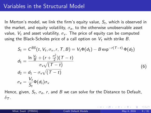
In Merton’s model, we link the firm’s equity value, St , which is observed inthe market, and equity volatility, σe , to the otherwise unobservable assetvalue, Vt and asset volatility, σv . The price of equity can be computedusing the Black-Scholes price of a call option on Vt with strike B.

St = CBS(t,Vt , σv , r ,T ,B) = VtΦ(d1)− B exp−r(T−t) Φ(d2)

d1 =ln Vt

B + (r + σ2v2 )(T − t)

σv√

(T − t)

d2 = d1 − σv√

(T − t)

σe =Vt

StΦ(d1)σv

(6)

Hence, given, St , σe , r , and B we can solve for the Distance to Default,δT .


Credit Spreads in Merton’s Model

Merton’s model can also be used to compute the credit spread above theyield of a risk-free bond.Let Pr (t,T ) be the price of a risk-free zero coupon bond maturing at timeT . Let Pd(t,T ) be the price of a corporate risky bond maturing at timeT . Then, we can define the credit spread on their yields, assumingcontinuous compounding, as,

spread(t,T ) =1

T − tln

Pd(t,T )

Pr (t,T )(7)

In Merton’s model the price of firm’s debt can be computed as adiscounted value of default-free debt, B, and a Black-Scholes price of ashort put option on Vt with strike, B. This gives,

Pd(t,T ) = Pr (t,T )Φ(d2) +Vt

BΦ(d1) (8)

Plugging this back into Equation 7 gives us the formula for the creditspread.


Evaluation of Merton’s Model

Advantages

Credit Risk of a firm is connected to underlying structural variables.

Intuitive Economic Explanation and Endogenous explanation of creditdefaults.

Option Analogy allows for easy implementation.

Disadvantages

Too Simplistic: Equity as Call option, Debt matures at same time.

Only applicable if a firm has tradable equity and a good estimate ofdebt level. Not extendable for private firms or sovereigns.

Assumes that two equally leveraged firms with identical marketcapitalization and asset volatility are of equal risk.

Underestimate credit spreads for short time to maturity that isempirically difficult to explain.


KMV Extension of Merton’s Model

KMV (now Moody’s KMV) model was developed in 1990s and it focusedon modelling defaults by extending the Merton Model.

Mapped Distance to Default to historical default rates usingproprietary database.

Removed the need to model credit risk using Option Theory.

KMV model is only focused on modelling default and not the creditspreads.


Dynamics of the KMV Model - EDF

One of the central ideas in the KMV model is the Expected DefaultFrequency (EDF). This is the one-year probability of default of an obligor.Going back to Merton’s model the EDF would be,

EDFMerton = 1− Φ

(ln V0

B + (µv − σ2v2 )

σv

)(9)

In KMV model, the EDF has similar structure to the Merton model butthe function 1− Φ is replaced with an estimated KMV function. Thevariable µv is ignored and the V0 and σv are backed out from theobservable value of equity of the firm.

The default boundary, B, is 12 of short-term debt (< 1 year) and

100% of long-term debt.

Floor on the Estimated 1 year default probability of 40% and a ceilingof 0.01%.


Dynamics of the KMV Model - DD

The other central idea in the KMV model is the Distance to Default (DD).To put it simply, a higher DD means a firm is less likely to default than alower DD.

The DD is mapped to EDF using empirical proprietary KMVdatabase. Firms with equal DD have equal EDF.

DD in the KMV model can be expressed by the following equation,

DD =(V0 − F )

σvV0(10)

where F is the default threshold.

Relationship between EDF and DD. (Source: Moody’s/KMV)


Ratings Based Models

Credit Rating measures the credit quality of a firm at any given point intime. The Ratings based model computes the probabilities of this ratingchanging. These migration probabilities are supplied by Rating Agencies(for e.g., Moody’s, Standard and Poor’s). JP Morgan CreditMetrics is apopular ratings based credit risk model.

In the KMV model the fundamental state variable was DD, in theRatings Migration approach the state variable is the Credit Rating.

Firms with equal Credit Rating have equal migration probabilities.

Rating agencies have huge database that cover a wide range of firmsincluding sovereigns.

Rating agencies focus on ”through the cycle” credit ratings causingless fluctuations as opposed to KMV which is ”point in time”.

Rating agencies are slow to react to credit events leading to a lagfrom the market spreads.


An Example Ratings Migration Matrix

One year Transition Probability Matrix taken from Moody’s. (Source:Elton E, Gruber M, Agrawal D, Explaining the Rate Spread on CorporateBonds, Journal of Finance 2001)


Migration Model in Firm Value Model

Popular way to embed a migration model inside a firm value model.

Suppose we are given transition probabilities by the rating agenciesfor n rating classes. Denote pj where 0 ≤ j ≤ n as the probability fora given firm to be in rating class j . We then select rating migrationthresholds −∞ = d0 < d1 < .... < dn < dn+1 =∞ such thatP(dj−1 < Vt < dj) = pj ∀j .If we assume that the asset process, Vt , has log normal distribution(Merton’s assumption), then we can compute the thresholds usingstandard normal distribution as,

d1 = ZCCC = Φ−1(pdef )

d2 = ZB = Φ−1(pdef + pCCC )

d3 = ZBB = Φ−1(pdef + pCCC + pB)

...

(11)


Multivariate Firm Value Model

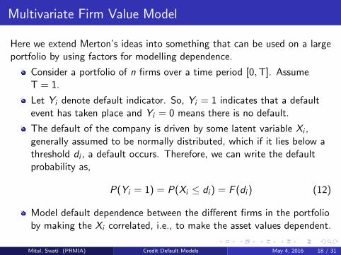
Here we extend Merton’s ideas into something that can be used on a largeportfolio by using factors for modelling dependence.

Consider a portfolio of n firms over a time period [0,T]. AssumeT = 1.

Let Yi denote default indicator. So, Yi = 1 indicates that a defaultevent has taken place and Yi = 0 means there is no default.

The default of the company is driven by some latent variable Xi ,generally assumed to be normally distributed, which if it lies below athreshold di , a default occurs. Therefore, we can write the defaultprobability as,

P(Yi = 1) = P(Xi ≤ di ) = F (di ) (12)

Model default dependence between the different firms in the portfolioby making the Xi correlated, i.e., to make the asset values dependent.


Generic Factor Model

Let X = (X1 X2...Xn)T , then the random vector X is driven by a set of(p << n) factors to reduce the dimensionality of the correlation matrix. Ageneric factor model can be expressed as,

X = α + βT F + ε (13)

α ∈ Rn is a vector of constants that can be thought of as the globalfactor affecting all firms.

F ∈ Rp is a random vector of (systematic or economic) factors.

βT ∈ Rn×p is the factor loading on the p factors since each Xi loaddifferently on each factor.

ε ∈ Rn is a random vector of (idiosyncratic) terms and are henceuncorrelated with mean zero.

cov(F , ε) = 0


Gaussian Linear Factor Model

Since the firm value model descends from Merton model, we assume thatX has a multivariate normal distribution.

Let F ∼ N(0,Ω)

Let ε ∼ N(0, Γ)

Then, X ∼ N(α,βTΩβ + Γ)

cov(Xi ,Xj) = βTi Ωβj

For majority of credit risk models, since actual asset values of the companyare unobservable, the factors are derived by observing the equity returns.


One Factor Vasicek Model

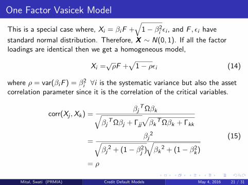
This is a special case where, Xi = βiF +√

1− β2i εi , and F , εi have

standard normal distribution. Therefore, X ∼ N(0, 1). If all the factorloadings are identical then we get a homogeneous model,

Xi =√ρF +

√1− ρεi (14)

where ρ = var(βiF ) = β2i ∀i is the systematic variance but also the assetcorrelation parameter since it is the correlation of the critical variables.

corr(Xj ,Xk) =βj

TΩβk√βj

TΩβj + Γjj

√βk

TΩβk + Γkk

=βj

2√βj

2 + (1− β2j )√βk

2 + (1− β2k)

= ρ

(15)


Bernoulli Mixture Model

We start with a portfolio of n firms and a p-dimensional factor vectorΘ = (θ1, θ2, ..., θp). In a Bernoulli Mixture Model, the probability ofdefault conditional on these factors is given by,

P(Yi = 1|Θ = Θ) = pi (Θ) (16)

such that the joint probability of the default indicators conditional on thefactors is given by,

P(Y1 = y1,Y2 = y2, ...,Yn = yn|Θ = Θ) =n∏

i=1

pi (Θ)yi (1− pi (Θ))1−yi

(17)And, hence, the default indicators of the n firms are independentconditional on the factor vector with their joint default probability given by,

P(Y1 = 1,Y2 = 1, ...,Yn = 1|Θ) =n∏

i=1

pi (Θ) (18)


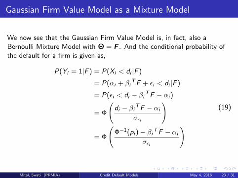
Gaussian Firm Value Model as a Mixture Model

We now see that the Gaussian Firm Value Model is, in fact, also aBernoulli Mixture Model with Θ = F . And the conditional probability ofthe default for a firm is given as,

P(Yi = 1|F ) = P(Xi < di |F )

= P(αi + βiTF + εi < di |F )

= P(εi < di − βi TF − αi )

= Φ

(di − βi TF − αi

σεi

)

= Φ

(Φ−1(pi )− βi TF − αi

σεi

)(19)


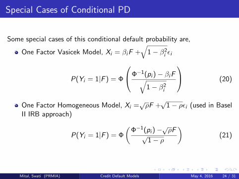
Special Cases of Conditional PD

Some special cases of this conditional default probability are,

One Factor Vasicek Model, Xi = βiF +√

1− β2i εi

P(Yi = 1|F ) = Φ

Φ−1(pi )− βiF√1− β2i

(20)

One Factor Homogeneous Model, Xi =√ρF +

√1− ρεi (used in Basel

II IRB approach)

P(Yi = 1|F ) = Φ

(Φ−1(pi )−

√ρF

√1− ρ

)(21)


Copulas

Definition

Let C be a copula function. Then C : [0, 1]n → [0, 1] such that there arerandom variables U1,U2, ...,Un that take values on [0, 1] whose jointcumulative distribution function is C .

C (u1, u2, ..., un) = P(U1 ≤ u1,U2 ≤ u2, ...,Un ≤ un) (22)

Multivariate Distribution using Copula

Consider a vector of random variables (X1,X2, ...,Xn) such that theirunivariate marginal distribution functions are (F1(x1),F2(x2), ...,Fn(xn)).Then the Copula function results in their multivariate joint distribution,

C (F1(x1),F2(x2), ...,Fn(xn)) = F (x1, x2, ..., xn) (23)

Sklar’s Theorem established that any multivariate distribution F can bewritten in this form using a Copula Function.


Copula Functions

Gaussian and t-copula are two of the most common Copula functions usedin Credit Default Models. We define them as follows,

Gaussian Copula

Let Φn be Multivariate Normal Distribution, then we can define theGaussian Copula as,

C (u1, u2, ..., un) = Φn(Φ−1(u1),Φ−1(u2), ...,Φ−1(un),ρ) (24)

Student’s t Copula

Let Tν and tν be the multivariate and univariate Student’s t distributionwith ν degrees of freedom.Then, we define the Student’s t Copula as,

C (u1, u2, ..., un) = Tν(t−1ν (u1), t−1ν (u2), ..., t−1ν (un),ρ) (25)


Default Correlation Models

Modelling default dependence for credit portfolios using Copulas waspopularized by Li in [2]. We build our framework with the followingassumptions.

We have n firms and we want to model their default correlations overa fixed time period [0,T ].

We have the marginal distribution of survival times, Si , for each ofthese firms. Denote this by Fi (s) = P(Si ≤ s).

Then Copulas are one of the ways to model the joint distributionfunction of the survival times,

F (s1, s2, ..., sn) = C (F1(s1),F2(s2), ...,Fn(sn), ρ) (26)

Therefore, for C = Φn, the joint default probability is given by,

P(S1 < T , ...,Sn < T ) = Φn(Φ−1(F1(S1)), ...,Φ−1(Fn(Sn)),ρ) (27)

For C = Tν , the joint default probability is,

P(S1 < T , ...,Sn < T ) = Tν(t−1ν (F1(S1)), ..., t−1ν (Fn(Sn)),ρ) (28)


Factor Model with Gaussian Copula

Let us look again at the One-Factor Vasicek Model covered earlier. Weknow that the default probability is given by Fi (Si ) = P(Si < T ) = pi andthe joint default probability distribution is given as,

P(Y1 = 1, ...,Yn = 1) = Φn(Φ−1(p1), ...,Φ−1(pn),ρ) (29)

In the factor model, the defaults are conditionally independent on thesystematic factors, Q, and therefore the latent variables,

Xi =√βi Q +

√1− β2i εi , have conditional joint default probability given

by the copula function,

C (p1, p2, ..., pn) =

∫ +∞

−∞

n∏i=1

Φ

Φ−1(pi )− βiQ√1− β2i

φ(y)dy (30)


Conclusions

We have looked at the dynamics of different credit default models startingfrom Firm Value models to Multivariate Factor Models.

All sophisticated banks have advanced IRB models for computingDefault Risk on credit portfolios. Generally, multifactor model withcopula dependence structure is well understood and widelyimplemented.

We discussed the dynamics of different credit risk models. One of theother big challenges is in the calibration of these models. Forexample: factor selection, factor weights, correlation structure etc.

In order to compute the distribution of default loss, Monte Carlotechniques are typically used. There are many computationalchallenges in a Monte Carlo simulation especially for non-linearproducts that require full revaluation.


Reference (1/2)

McNeil AJ, Frey R and Embrechts P: Quantitative Risk Management:Concepts, Techniques and Tools (Revised Edition). PrincetonUniversity Press., 2015

Crouhy M., Galai D., Mark R: A Comparative analysis of currentcredit risk models, 2000

Crosbie, P: Modeling Default Risk, Moody’s KMV TechnicalDocument, 2002

Kealhofer, S. and Bohn, J.: Portfolio management of default risk,Moody’s KMV Technical Document, 2001


Reference (2/2)

Rutkowski, M. and Tarca, S., Regulatory Capital Modelling for CreditRisk, University of Sydney, 2014

Li, D. X. On default correlation: A copula function approach. Journalof Fixed In- come 9(4), 43–54., 2000.

Tarashev N. and Zhu H., Specification and Calibration Errors inMeasures of Portfolio Credit Risk: The Case of the ASRF Model,Bank of International Settlements


credit default models

Economy & Finance