credit derivatives insights and index...
TRANSCRIPT

FOURTH EDITION 2008
Handbook of Single Nameand Index StrategiesCredit Derivatives Insights
R E S E A R C H
Primary Analysts
Sivan MahadevanVishwanath TirupatturAshley MusfeldtAndrew SheetsPhanikiran Naraparaju

The Credit Derivatives Insights Series
The Handbook of Single Name and Index Strategies, now in its fourthprinting, contains select previously published research reports on creditinvestment strategies, credit derivatives instruments and valuation techniquesfrom our Credit Derivatives Insights publications. It also contains “primers”on credit derivatives concepts and a glossary with brief definitions for nearly150 terms used in the market. We have organized the book into six broadsections: instruments and primers, valuation and investment frameworks,basis ideas, credit curves, options and embedded options, and credit marketthemes. There are 74 chapters in all.
The Fourth Edition–What’s New?
This fourth edition contains 13 new and numerous revised chapters focusedon a variety of topics. Given the immense size of the market as it experiencesanother turn in the credit cycle, we include material on the shift in thebalance of power among CDS users and our thoughts on operationalchallenges and new counterparty risks in the system. Innovation in themarket continues, and we include new material on residential propertyderivatives and CDS referencing both European sovereigns and USmunicipalities. As the option markets continue to grow, we include bothprimer material and strategic ideas linked to the index options markets. Therapidly developing stress in the credit markets motivated new material onbasis trades, credit curve relationships and LCDS dynamics with higherdefault rates, loan cancellations and the introduction of new LCDS indices.
We hope Morgan Stanley clients find this handbook useful, and we welcomeany feedback so that we can improve future editions.
FOURTH EDITION 2008
CreditDerivativesInsightsHandbook of Single Name andIndex Strategies
Primary Analysts: Sivan Mahadevan Vishwanath Tirupattur Ashley Musfeldt Andrew Sheets Phanikiran Naraparaju
The Primary Analyst(s) identified above certify that the views expressed in this report accurately reflect his/her/their personal views about the subject securities/instruments/issuers, and no part of his/her/their compensation was, is or will be directly or indirectly related to the specific views or recommendations contained herein.
This report has been prepared in accordance with our conflict management policy. The policy describes our organizational and administrative arrangements for the avoidance, management and disclosure of conflicts of interest. The policy is available at www.morganstanley.com/institutional/research.
Please see additional important disclosures at the end of this report.
Morgan Stanley & Co. Incorporated
February 26, 2008

Morgan Stanley Credit Derivatives Insights – Handbook of Single Name and Index Strategies
INTRODUCTION 1
SECTION A. GETTING STARTED: INSTRUMENTS AND PRIMERS
1 A PRIMER ON SINGLE NAME INSTRUMENTS & STRATEGIES 8
2 UNDERSTANDING SYNTHETIC STRUCTURED FINANCE – FIRST STEPS 20
3 CDS ON CDOS: BACK TO THE FUTURE 32
4 LEVERAGED LOAN CDS: A FIRST STEP UP 34
5 TRADING RECOVERY RISK – THE MISSING LINK 44
6 FLOATING A NEW IDEA – CMCDS 47
7 STANDARDIZED CDS INDICES – CDX, LCDX, ITRAXX, LEVX, ABX AND CMBX 50
8 SUCCEEDING IN AN ACTIVIST WORLD – SUCCESSION LANGUAGE 57
9 RANGE ACCRUAL PRIMER 60
10 INDEX OPTIONS PRIMER 64
11 MUNI MANIA 70
12 SOVEREIGN MANIA 74
SECTION B. VALUATION AND INVESTMENT FRAMEWORKS
13 VALUING CORPORATE CREDIT: QUANTITATIVE APPROACHES VS. FUNDAMENTAL ANALYSIS 78
14 LIBOR METRICS 95
15 A TALE OF TWO CREDIT MARKETS 97
16 MAKING A POINT – UPFRONT 99
17 MERTON VS. THE MARKET 101
18 THE SENIOR SUB DIVIDE 104
19 EQUITY INDICATORS – IS THE TAIL WAGGING THE DOG? 106
20 RECALIBRATING RELATIVE VALUE 109
21 LOOKING FORWARD TO CREDIT 111
22 LEANING AGAINST THE FORWARDS 114
23 CREDIT VOLATILITY – THE UNINTENDED CONSEQUENCES 118
24 VOLATILITY CONFUSES CREDIT SPREADS 121
25 THE SECRET OF MY SUCCESS(ION) 124
26 ”WORTHLESS” PROTECTION? 127
27 RECOVERY LESSONS 133
28 THE RECOVERY MARKET’S NEXT LEG – INDICES 136

SECTION B. VALUATION AND INVESTMENT FRAMEWORKS (cont'd)
29 WHAT EXACTLY IS INDEX ARB? 141
30 LCDS, AFTER THE TRADE 144
31 RPX DERIVATIVES: NEW HOUSING TOOLKIT 147
32 DOWNTURN DURATIONS 151
SECTION C. BASIS IDEAS
33 GETTING LONG ASYMMETRY 156
34 ASYMMETRY RELOADED 159
35 WHY IS THE BASIS NEGATIVE? 162
36 NEGATIVE BASIS POINTS 164
37 THE BASIS TODAY – OPTICS VS. OPPORTUNITY 167
38 LCDS – UNDERSTANDING THE BASIS 169
39 LCDS – WHAT’S THE RIGHT CALL? 174
40 THE HIGH YIELD BASIS – CALLING ALL BONDS 178
41 HIGH YIELD, HIGHER RATES, HELLO CONVEXITY 180
42 THE AIRLINE TRIANGLE 182
43 OIL RESHAPES THE AIRLINE TRIANGLE 184
44 TURNING A TRIANGLE INTO A SQUARE 187
45 STRETCHING THE AIRLINE TRIANGLE 189
46 LIBOR, THE BID AND THE BASIS 192
47 AUTO VOLATILITY TURNS TO AUTO CONVEXITY 195
48 PLAYING LBOS WITH CDS – DETAILS, DETAILS… 198
49 WHY IS THE BASIS STILL NEGATIVE? 201
SECTION D. CREDIT CURVES
50 GETTING SHORT THE LONG END 206
51 BASIS TRADING WITH STEEP CREDIT CURVES 209
52 PAINTING CREDIT CURVES – BROAD STROKES VS. FINE LINES 212
53 CURVE LESSONS FROM HIGH YIELD 215
54 STEEP CURVES, TECHNICAL BIDS AND THE BASIS 218
55 CURIOUS ABOUT CROSSOVER CURVES? 220
56 CREDIT CURVE REGIME SHIFT 224

Morgan Stanley Credit Derivatives Insights – Handbook of Single Name and Index Strategies
SECTION E. OPTIONS AND EMBEDDED OPTIONS
57 WATCHING VOLATILITY, TRADING VOLATILITY 228
58 SPREAD VOLATILITY – FINALLY SOMETHING TO SMILE ABOUT 231
59 SELLING TOMORROW’S TIGHTENING TODAY 234
60 UNDERSTANDING CORPORATE BOND OPTIONS – VALUATION ISSUES AND PORTFOLIO APPLICATIONS 237
61 OPTIONS FOR NOTHING, INTEREST RATE RISK FOR FREE 247
62 GETTING A HANDLE ON HIGH YIELD CALL RISK 249
63 COVERED CALLS AREN’T CROWDED TRADES 252
64 SO MUCH CONVEXITY, SO FEW OPTIONS 255
65 VOLATILITY GETS TECHNICAL TOO 258
66 CREDIT OPTIONS: NOT ON STRIKE 261
67 SO MANY OPTIONS, SO LITTLE TIME 264
SECTION F. CREDIT MARKET THEMES
68 MANIC COMPRESSION 268
69 RISK PREMIUM OR VIX PREMIUM? 271
70 DOES THE VIX REALLY MATTER? 274
71 DANA + DELPHI: WATCH THE COUNT AND THE ROLL 277
72 CONVEXITY, NOT COMPLEXITY 280
73 CDS EQUILIBRIUM SHIFT 284
74 STRESS TESTING THE CDS MARKET 287
SECTION G. GLOSSARY 292
Please see additional important disclosures at the end of this report. 1
Introduction
The ultimate measure of a man is not where he stands in moments of comfort and convenience, but where he stands at times of challenge and controversy.
– Martin Luther King Jr.
Well over a decade after its birth, the credit derivatives market has forced a secular change in the management of credit portfolios. The key motivator for the growth of the market was credit stress in many of the emerging markets during the middle to late 1990s, followed by a rather sharp turn in the corporate credit cycle in the earlier part of this decade. These events also served as good tests of contract specifications and led to standardization. In fact, standardization was the key driver of growth in most corners of the credit derivatives market, from single-name to structured credit, demonstrating that there was, indeed, a large amount of pent-up demand. With increased liquidity, convergence among many market instruments, and an active structured credit market, the conventional model of credit investing was challenged like never before. In the recent past, key themes included the risks and operational issues associated with the immense size of the market, new frontiers resulting from default swaps gaining acceptance in both the structured finance and leveraged loan worlds, and innovation in areas such as trading recovery risk.
© 2006 Morgan Stanley
Today as cyclical economic forces have repriced corporate credit substantially, both a terribly weak mortgage credit cycle and the bursting of the US housing bubble have put credit derivatives markets to a new set of tests.
A huge market is being challenged by operational risks, counterparty issues associated with growth in the hedge fund industry and the generally poor health of monoline insurers. Furthermore, the new credit derivative instruments, including those referencing ABS, CMBS and leveraged loans, are being tested in a negative credit environment for the first time. The addition of many non-traditional credit investors within the credit markets has changed the balance of credit flows and increased both the daily volumes and volatility of the popular credit derivatives indices dramatically.
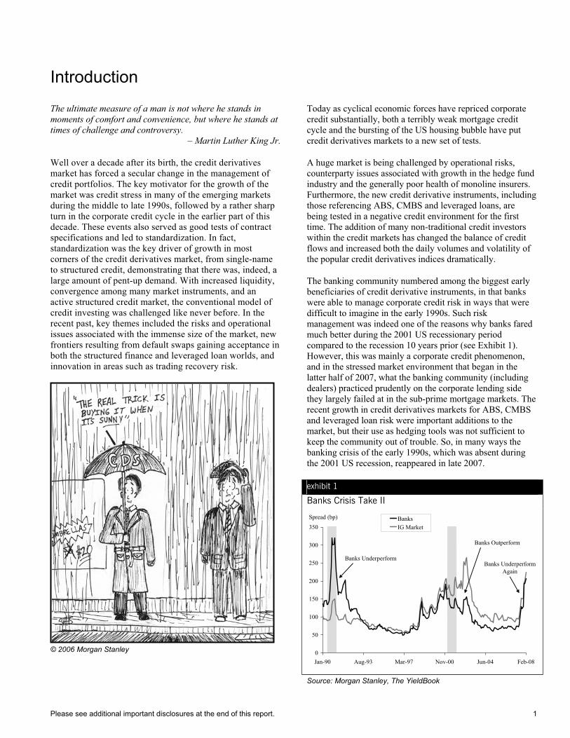
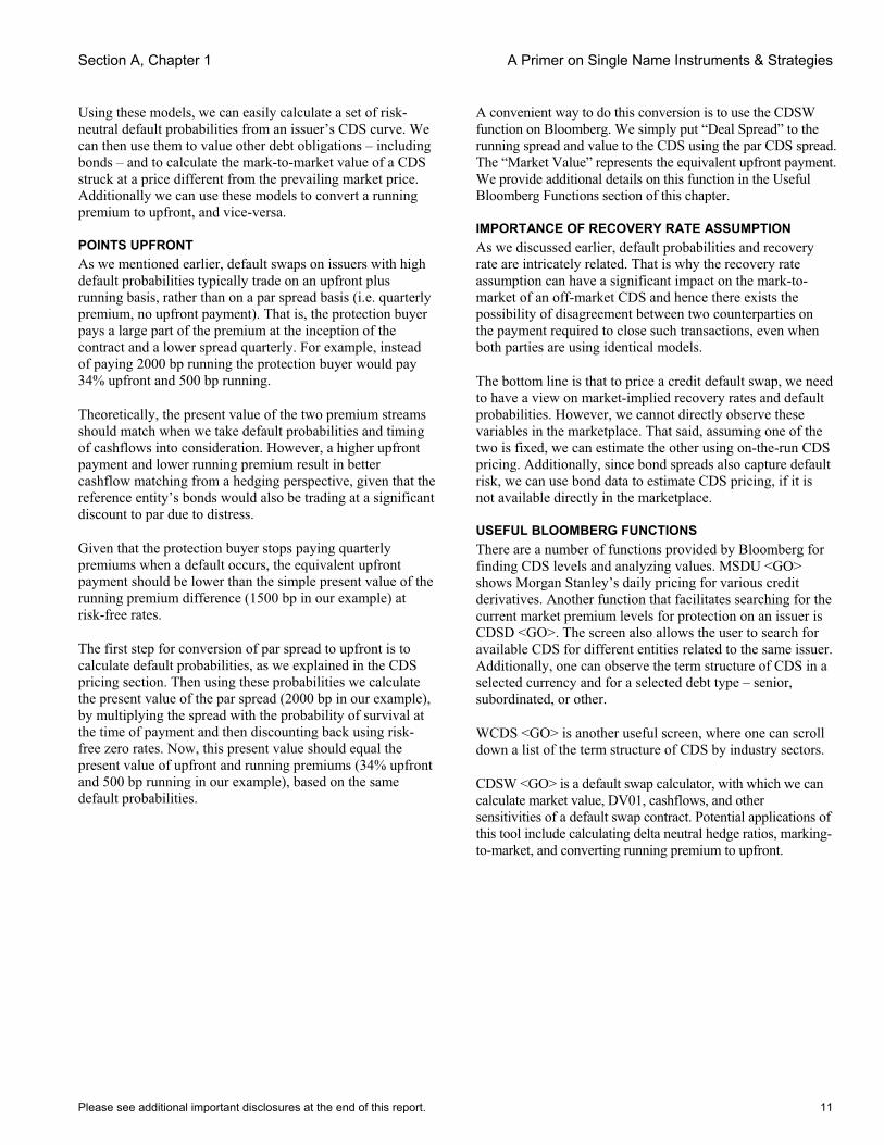
The banking community numbered among the biggest early beneficiaries of credit derivative instruments, in that banks were able to manage corporate credit risk in ways that were difficult to imagine in the early 1990s. Such risk management was indeed one of the reasons why banks fared much better during the 2001 US recessionary period compared to the recession 10 years prior (see Exhibit 1). However, this was mainly a corporate credit phenomenon, and in the stressed market environment that began in the latter half of 2007, what the banking community (including dealers) practiced prudently on the corporate lending side they largely failed at in the sub-prime mortgage markets. The recent growth in credit derivatives markets for ABS, CMBS and leveraged loan risk were important additions to the market, but their use as hedging tools was not sufficient to keep the community out of trouble. So, in many ways the banking crisis of the early 1990s, which was absent during the 2001 US recession, reappeared in late 2007.
exhibit 1
Banks Crisis Take II
Spread (bp)
0
50
100
150
200
250
300
350
Jan-90 Aug-93 Mar-97 Nov-00 Jun-04 Feb-08
BanksIG Market
Banks Underperform
Banks Outperform
Banks UnderperformAgain
Source: Morgan Stanley, The YieldBook
Morgan Stanley Credit Derivatives Insights – Handbook of Single Name and Index Strategies
2 Please see additional important disclosures at the end of this report.
LOOKS AND FEELS LIKE A BOND What most early users of credit derivatives wanted to achieve was rather simple: a transfer of credit risk from one party to another. The early instruments, including credit linked notes and total return swaps, achieved this, but they had their shortcomings, as they were generally linked to a single bond or loan and lacked liquidity. Credit default swaps, over time, gained popularity largely because they looked and felt like bonds and loans, yet were not tied specifically to one bond or loan. The restructuring credit event was a popular theme to debate among various members of the investment community; much of the standardization discussions centered on these debates.
© 2008 Morgan Stanley
THE EVOLUTION OF THE CREDIT DEFAULT SWAP While credit derivatives trading volumes are dominated today by contracts that reference corporate entities, for those who are not familiar with the early days of the markets, emerging markets sovereign credit was where the default swap first gained popularity in the mid-1990s. Default swaps offered a simple way to trade sovereign credit risk to various terms. Furthermore, with many hedge fund participants in emerging markets, the default swaps helped investors create outright short and long/short positions much more easily than by using bonds and the repo markets.
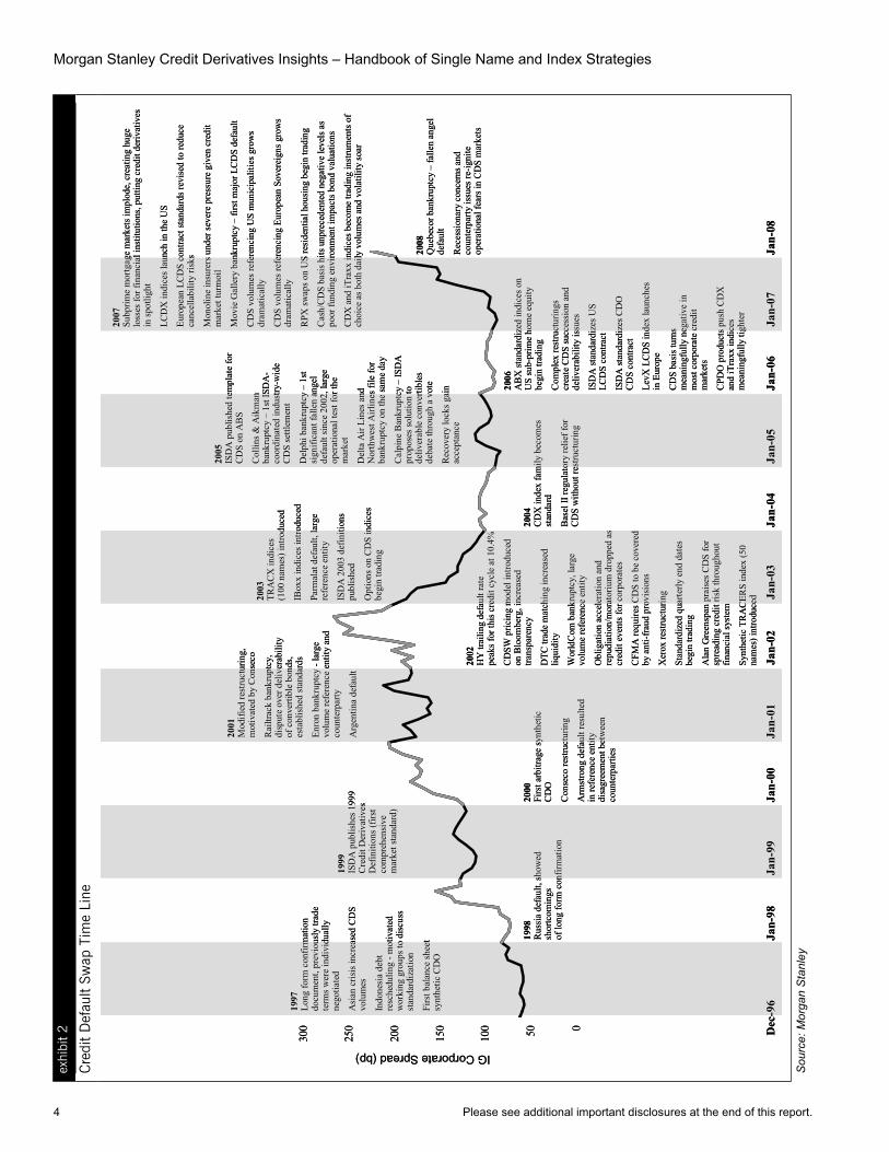
From 1997 through 2002, the credit default swap went through an incredible growing-up process, driven by a deteriorating credit cycle that made for good tests and resulted in standardization, which, in turn, spurred more liquidity and opportunities for further tests (see Exhibit 2). The Asian emerging markets events of 1997, including the rescheduling of some of Indonesia’s debt payments, motivated the creation of working groups to address standardization. In the same year, a standard (long form) confirmation gained acceptance. Prior to this, most trade terms were individually negotiated. Also, 1997 witnessed the first synthetic CDO, the beginning of a structured credit market that contributed hugely to liquidity. The shortcomings of the original definitions of restructuring were revealed on numerous occasions through credit events triggered by Russia, Conseco and Xerox. Ultimately, such tests prompted rethinking the restructuring credit events, resulting in modified restructuring, modified-modified restructuring, and even the growing use of no-restructuring credit events. Other credit events were equally important. The Armstrong default highlighted the importance of clearly specified reference entities (at the appropriate level in the capital structure), and the Railtrack bankruptcy motivated focus on specific details concerning the deliverability of convertible bonds. The Enron and WorldCom bankruptcies, along with the Parmalat and Argentina defaults, were good tests of the system in general, given the volume of contracts outstanding in each case and the number of counterparties involved (Enron was, itself, a counterparty).
Systems and procedures were important to the evolution of the credit default swap, as well. The Commodity Futures Modernization Act of 2000 (CFMA) required that default swaps be covered by anti-fraud measures, which created “walls” between lenders and hedgers in banking institutions. Depository Trust Company (DTC) trade matching helped increase liquidity dramatically, as did the introduction of the CDSW default swap pricing tool on the Bloomberg systems. Finally, the more recent injections of liquidity came from the near hyper-growth of trading in default swap indices, from TRACERSSM to the Dow Jones TRACXSM Index and IBoxx to the industry standardized CDX family of indices over the course of two years (2002 through 2004), aided by the birth of the credit hedge fund.
BIG DEFAULTS IN A BIG WORLD By the beginning of 2005, most would have argued that the corporate-credit-backed credit default swap was a relatively mature instrument, given the experience of numerous recession-period defaults and daily volume levels that were surpassing those of traditional corporate bonds. Yet, a decade after its birth, we would argue that events in 2005 were critical to the market, given the explosive volumes of outstanding risk driven both by the credit derivative indices and structured credit flows. The Collins & Aikman bankruptcy filing in mid-2005 represented the first CDX index constituent default (HY CDX), prompting the first

Introduction
Please see additional important disclosures at the end of this report. 3
ever industry-wide auction process, with over 400 institutional investors participating (see Chapter 7 for a description of this process). The bankruptcy filing of Delphi was the first significant US fallen angel default since 2002 and a name that appeared in both investment grade CDX index tranches and in nearly one-third of all outstanding bespoke synthetic CDOs.
Other significant 2005 credit events included two US airlines filing for bankruptcy literally within minutes of one another (Delta Air Lines and Northwest Airlines), and Calpine, a large US power company present in all of the HY CDX indices, with a complicated capital structure that brought into question the deliverability of certain convertible securities. Ultimately the ISDA protocol for CDS settlement determined which bonds would be deliverable (via the protocol), and the auction was conducted. The Dana and Dura fallen angel defaults in 2006 were easily executed through the ISDA protocol, and in 2007 the Movie Gallery default was the first one to be settled for LCDS contracts using the protocol. In early 2008, Quebecor represented the first big fallen angel default since the auto defaults of 2005-2006.
© 2008 Morgan Stanley
NEW FRONTIERS Quite a bit of CDS innovation has occurred over the past three years. Within the corporate credit space, recovery locks, instruments that allow investors to hedge recovery risk alone, have gained popularity recently, providing an interesting
alternative to traditional CDS (see Chapters 5, 27 and 28). In the high yield space, secured loan CDS (LCDS) standards emerged in 2004–2005 in Europe and the US, and the market has enjoyed quite a bit of growth since (see Chapter 4). Furthermore, the market is developing an appetite for options on single-name CDS and CDS indices. Within the securitized products space, 2005 and 2006 saw the establishment of ISDA standards for CDS on structured finance securities, including asset-backed securities, commercial real estate securities and cash CDOs (see Chapters 2 and 3). In early 2006, we saw the launch of the ABX indices (US residential sub-prime credit) and CMBX (commercial real estate credit). In late 2006, the LevX indices covering European leveraged loans (via LCDS contracts) was launched, and in 2007 a US version of this index (LCDX) began trading as well. Also in 2007, CDS contracts referencing both European sovereign issuers and US municipalities gained prominence as trading volumes grew substantially.
DETAILS MATTER An important credit derivatives theme involves sorting out all of the details behind the recent innovation, and even some of the older standards. In the investment grade corporate credit space, there has been a lot of focus on “succession” issues of CDS contracts, given the high volumes of corporate restructuring activity (see Chapters 8 and 25). In fact, there are numerous situations where CDS can be left with no deliverable obligations, which has led to some significant repricings (see Chapter 26). There has also been a lot more trading activity in credit curves in the corporate credit space. Within the recently standardized LCDS contracts, there has been much discussion about restructuring issues and cancellability, but as the market further develops, we expect to see some convergence here.
SUBPRIME WOES The biggest test for the CDS market today is not so much in corporate credit risk, which has dominated this market for years, but in the US mortgage markets, where a still young derivatives market is meeting an unprecedented weak mortgage credit and housing cycle head-on. There are contract details that are being tested now, as well as monetization issues for some of these swaps (as their market values change dramatically) and counterparty issues. The contagion of sub-prime risk into the broader financial system introduced a systemic crisis that resulted in unprecedented trading volumes and helped to push forward the development of new CDS contracts (on European sovereigns and US municipalities) and bigger trading volumes in CDS options linked to the standardized indices.
Morgan Stanley Credit Derivatives Insights – Handbook of Single Name and Index Strategies
4 Please see additional important disclosures at the end of this report.
exhi
bit
2
Cre
dit
Def
ault
Swap
Tim
e Li
ne
050100
150
200
250
300
Jan-
07
2007
Subp
rime
mor
tgag
e m
arke
ts im
plod
e, c
reat
ing
huge
lo
sses
for f
inan
cial
insti
tutio
ns, p
uttin
g cr
edit
deriv
ativ
es
in sp
otlig
ht
LCD
X in
dice
s lau
nch
in th
e U
S
Euro
pean
LC
DS
cont
ract
stan
dard
s rev
ised
to re
duce
ca
ncel
labi
lity
risks
Mon
olin
ein
sure
rs u
nder
seve
re p
ress
ure
give
n cr
edit
mar
ket t
urm
oil
Mov
ie G
alle
ry b
ankr
uptc
y –
first
maj
or L
CD
S de
faul
t
CD
S vo
lum
es re
fere
ncin
g U
S m
unic
ipal
ities
gro
ws
dram
atic
ally
CD
S vo
lum
es re
fere
ncin
g Eu
rope
an S
over
eign
s gro
ws
dram
atic
ally
RPX
swap
s on
US
resi
dent
ial h
ousin
g be
gin
tradi
ng
Cas
h/C
DS
basi
s hits
unp
rece
dent
ed n
egat
ive
leve
ls a
s po
or fu
ndin
g en
viro
nmen
t im
pact
s bon
d va
luat
ions
CD
X a
nd iT
raxx
indi
ces b
ecom
e tra
ding
inst
rum
ents
of
choi
ce a
s bot
h da
ily v
olum
es a
nd v
olat
ility
soar
1997
Long
form
con
firm
atio
n do
cum
ent,
prev
ious
ly tr
ade
term
s wer
e in
divi
dual
ly
nego
tiate
d
Asi
an c
risis
incr
ease
d C
DS
volu
mes
Indo
nesi
a de
bt
resc
hedu
ling
-mot
ivat
ed
wor
king
gro
ups t
o di
scus
s st
anda
rdiz
atio
n
Firs
t bal
ance
shee
t sy
nthe
tic C
DO
Dec
-96
Jan-
98
1999
ISD
A p
ublis
hes 1
999
Cre
dit D
eriv
ativ
es
Def
initi
ons (
first
com
preh
ensi
ve
mar
ket s
tand
ard)
Jan-
00Ja
n-99
2001
Mod
ified
rest
ruct
urin
g,
mot
ivat
ed b
y C
onse
co
Rai
ltrac
kba
nkru
ptcy
, di
sput
e ov
er d
eliv
erab
ility
of
con
verti
ble
bond
s, es
tabl
ishe
d sta
ndar
ds
Enro
n ba
nkru
ptcy
-la
rge
vo
lum
e re
fere
nce
entit
y an
d co
unte
rpar
ty
Arg
entin
a de
faul
t
Jan-
02Ja
n-01
2003
TRA
CX
indi
ces
(100
nam
es) i
ntro
duce
d
IBox
xin
dice
s int
rodu
ced
Parm
alat
defa
ult,
larg
e re
fere
nce
entit
y
ISD
A 2
003
defin
ition
s pu
blis
hed
Opt
ions
on
CD
S in
dice
s be
gin
tradi
ng
Jan-
04Ja
n-03
2005
ISD
A p
ublis
hed
tem
plat
e fo
r C
DS
on A
BS
Col
lins &
Aik
man
ba
nkru
ptcy
–1s
t ISD
A-
coor
dina
ted
indu
stry
-wid
e C
DS
settl
emen
t
Del
phi b
ankr
uptc
y –
1st
sign
ifica
nt fa
llen
ange
l de
faul
t sin
ce 2
002,
larg
e op
erat
iona
l tes
t for
the
mar
ket
Del
ta A
ir Li
nes a
nd
Nor
thw
est A
irlin
es fi
le fo
r ba
nkru
ptcy
on
the
sam
e da
y
Cal
pine
Ban
krup
tcy
–IS
DA
pr
opos
es so
lutio
n to
de
liver
able
con
verti
bles
de
bate
thro
ugh
a vo
te
Rec
over
y lo
cks g
ain
acce
ptan
ce
Jan-
06Ja
n-05
1998
Rus
sia d
efau
lt, sh
owed
sh
ortc
omin
gs
of lo
ng fo
rm c
onfir
mat
ion
2002
HY
trai
ling
defa
ult r
ate
peak
s for
this
cre
dit c
ycle
at 1
0.4%
CD
SW p
ricin
g m
odel
intro
duce
d on
Blo
ombe
rg, i
ncre
ased
tra
nspa
renc
y
DTC
trad
e m
atch
ing
incr
ease
d liq
uidi
ty
Wor
ldC
om b
ankr
uptc
y, la
rge
volu
me
refe
renc
e en
tity
Obl
igat
ion
acce
lera
tion
and
repu
diat
ion/
mor
ator
ium
dro
pped
as
cred
it ev
ents
for c
orpo
rate
s
CFM
A re
quire
s CD
S to
be
cove
red
by a
nti-f
raud
pro
visi
ons
Xer
ox re
stru
ctur
ing
Stan
dard
ized
qua
rterly
end
dat
es
begi
n tra
ding
Ala
n G
reen
span
pra
ises
CD
S fo
r sp
read
ing
cred
it ris
k th
roug
hout
fin
anci
al sy
stem
Synt
hetic
TR
AC
ERS
inde
x (5
0 na
mes
) int
rodu
ced
2000
Firs
t arb
itrag
e sy
nthe
tic
CD
O
Con
seco
rest
ruct
urin
g
Arm
stro
ng d
efau
lt re
sulte
d in
refe
renc
e en
tity
disa
gree
men
t bet
wee
n co
unte
rpar
ties
2004
CD
X in
dex
fam
ily b
ecom
es
stan
dard
Bas
el II
regu
lato
ry re
lief f
or
CD
S w
ithou
t res
truct
urin
g
2006
AB
X st
anda
rdiz
ed in
dice
s on
US
sub-
prim
e ho
me
equi
ty
begi
n tra
ding
Com
plex
rest
ruct
urin
gs
crea
te C
DS
succ
essi
on a
nd
deliv
erab
ility
issu
es
ISD
A st
anda
rdiz
es U
S LC
DS
cont
ract
ISD
A st
anda
rdiz
es C
DO
C
DS
cont
ract
LevX
LCD
S in
dex
laun
ches
in
Eur
ope
CD
S ba
sis t
urns
m
eani
ngfu
lly n
egat
ive
in
mos
t cor
pora
te c
redi
t m
arke
ts
CPD
O p
rodu
cts p
ush
CD
X
and
iTra
xxin
dice
s m
eani
ngfu
lly ti
ghte
r
IG Corporate Spread (bp)
2008
Que
beco
r ban
krup
tcy
–fa
llen
ange
l de
faul
t
Rec
essi
onar
y co
ncer
ns a
nd
coun
terp
arty
issu
es re
-igni
te
oper
atio
nal f
ears
in C
DS
mar
kets
Jan-
08
Sou
rce:
Mor
gan
Sta
nley
Introduction
Please see additional important disclosures at the end of this report. 5
THE CREDIT DERIVATIVES INSIGHTS SERIES The Handbook of Single Name and Index Strategies, now in its fourth printing, contains select previously published research reports on credit investment strategies, credit derivatives instruments and valuation techniques from our Credit Derivatives Insights publications. It also contains “primers” on credit derivatives concepts and a glossary with brief definitions for nearly 150 terms used in the market. We have organized the book into six broad sections: instruments and primers, valuation and investment frameworks, basis ideas, credit curves, options and embedded options, and credit market themes. There are 74 chapters in all.
THE FOURTH EDITION – WHAT’S NEW? This fourth edition contains 13 new and numerous revised chapters focused on a variety of topics. Given the immense size of the market as it experiences another turn in the credit cycle, we include material on the shift in the balance of power among CDS users and our thoughts on operational challenges and new counterparty risks in the system. Innovation in the market continues, and we include new material on residential property derivatives and CDS referencing both European sovereigns and US municipalities. As the option markets continue to grow, we include both primer material and strategic ideas linked to the index options markets. The rapidly developing stress in the credit markets motivated new material on basis trades, credit curve
relationships and LCDS dynamics with higher default rates, loan cancellations and the introduction of new LCDS indices.
We hope Morgan Stanley clients find this handbook useful, and we welcome any feedback so that we can improve future editions.
ACKNOWLEDGEMENTS We would like to acknowledge the many other Morgan Stanley team members who were involved in some of the articles included in this handbook, including Anisha Ambardar, Lindsey Burnett, Jocelyn Chu, Payal Dave, Howard Esaki, Viktor Hjort, Rizwan Hussain, Suneet Joshi, Ravi Khushalani, Young-Sup Lee, Neil McLeish, Mohsin Naqvi, Rachel Ng, Gregory Peters, Simmi Sareen, Javier Serna, Ragini Shah, Praveen Singh, and Sejal Vora. We would also like to acknowledge our credit derivatives businesses within Morgan Stanley, whose team members have played a significant role in development of these markets, permitting investors and researchers to take a strategic approach to the markets. We would like to thank our creative services team, especially Dan Long, Patrick Oliver and Linda Warnasch, for their assistance in preparing this handbook. Finally, we very much appreciate the immeasurable amount of feedback that we have received on our reports from Morgan Stanley clients.


Section A
Getting Started: Instruments and Primers
Morgan Stanley Credit Derivatives Insights – Handbook of Single Name and Index Strategies
8 Please see additional important disclosures at the end of this report.
Chapter 1
A Primer on Single Name Instruments & Strategies
Primary Analyst: Sivan Mahadevan Primary Analyst: Peter Polanskyj
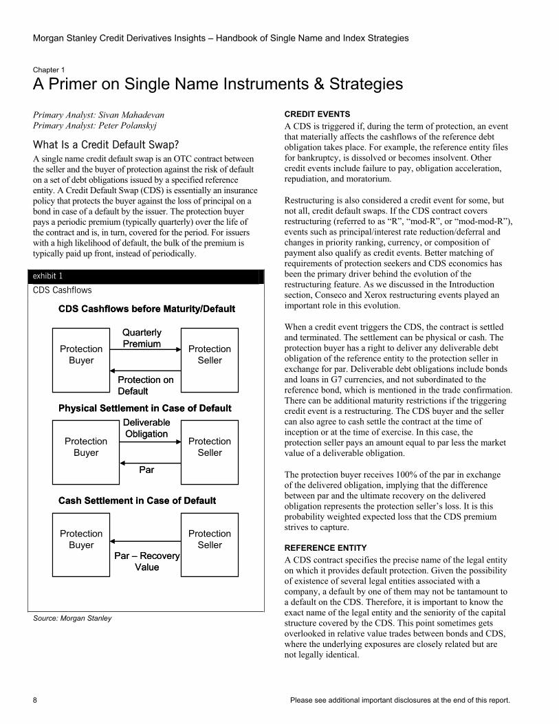
What Is a Credit Default Swap? A single name credit default swap is an OTC contract between the seller and the buyer of protection against the risk of default on a set of debt obligations issued by a specified reference entity. A Credit Default Swap (CDS) is essentially an insurance policy that protects the buyer against the loss of principal on a bond in case of a default by the issuer. The protection buyer pays a periodic premium (typically quarterly) over the life of the contract and is, in turn, covered for the period. For issuers with a high likelihood of default, the bulk of the premium is typically paid up front, instead of periodically.
exhibit 1
CDS Cashflows
Protection Buyer
Protection Seller
Quarterly Premium
Protection on Default
CDS Cashflows before Maturity/Default
Protection Buyer
Protection Seller
DeliverableObligation
Par
Physical Settlement in Case of Default
Protection Buyer
Protection Seller
Par – RecoveryValue
Cash Settlement in Case of Default
Protection Buyer
Protection Seller
Quarterly Premium
Protection on Default
CDS Cashflows before Maturity/Default
Protection Buyer
Protection Seller
DeliverableObligation
Par
Physical Settlement in Case of Default
Protection Buyer
Protection Seller
Par – RecoveryValue
Cash Settlement in Case of Default
Source: Morgan Stanley
CREDIT EVENTS A CDS is triggered if, during the term of protection, an event that materially affects the cashflows of the reference debt obligation takes place. For example, the reference entity files for bankruptcy, is dissolved or becomes insolvent. Other credit events include failure to pay, obligation acceleration, repudiation, and moratorium.
Restructuring is also considered a credit event for some, but not all, credit default swaps. If the CDS contract covers restructuring (referred to as “R”, “mod-R”, or “mod-mod-R”), events such as principal/interest rate reduction/deferral and changes in priority ranking, currency, or composition of payment also qualify as credit events. Better matching of requirements of protection seekers and CDS economics has been the primary driver behind the evolution of the restructuring feature. As we discussed in the Introduction section, Conseco and Xerox restructuring events played an important role in this evolution.
When a credit event triggers the CDS, the contract is settled and terminated. The settlement can be physical or cash. The protection buyer has a right to deliver any deliverable debt obligation of the reference entity to the protection seller in exchange for par. Deliverable debt obligations include bonds and loans in G7 currencies, and not subordinated to the reference bond, which is mentioned in the trade confirmation. There can be additional maturity restrictions if the triggering credit event is a restructuring. The CDS buyer and the seller can also agree to cash settle the contract at the time of inception or at the time of exercise. In this case, the protection seller pays an amount equal to par less the market value of a deliverable obligation.
The protection buyer receives 100% of the par in exchange of the delivered obligation, implying that the difference between par and the ultimate recovery on the delivered obligation represents the protection seller’s loss. It is this probability weighted expected loss that the CDS premium strives to capture.
REFERENCE ENTITY A CDS contract specifies the precise name of the legal entity on which it provides default protection. Given the possibility of existence of several legal entities associated with a company, a default by one of them may not be tantamount to a default on the CDS. Therefore, it is important to know the exact name of the legal entity and the seniority of the capital structure covered by the CDS. This point sometimes gets overlooked in relative value trades between bonds and CDS, where the underlying exposures are closely related but are not legally identical.
Section A, Chapter 1 A Primer on Single Name Instruments & Strategies
Please see additional important disclosures at the end of this report. 9
The Armstrong default was a case in point, as knowing the appropriate level in the capital structure covered by the CDS turned out to be key in determining which obligations were protected against default. We will discuss relative value trading in the Basis section of this primer.
On a related topic, changes in ownership of the reference entity’s bonds or loans can also result in a change in the reference entity covered by the CDS contract. The following table summarizes how the new reference entity is determined depending on the level of ownership changes:
exhibit 2
New Reference Entity When Ownership Changes
Ownership of bonds/loans New reference entity One entity assumes more than 75% Successor No entity assumes more than 75%, but
one of more entities assume 25-75% Divide the contract equally
among such entities No entity assumes more than 25% Original legal entity
Source: ISDA
If the legal entity does not survive, the CDS contract follows the entity that succeeds to highest percentage of bonds or loans.1
STANDARDIZED PAYMENT DATES Since 2002, a vast majority of CDS contracts have standardized quarterly payment and maturity dates to the 20th of March, June, September and December. This standardization has several benefits, including convenience in offsetting CDS trades, rolling over of contracts, relative value trading, single name versus the benchmark indices or tranched index products trading, etc.
1Please refer to Chapter 8.
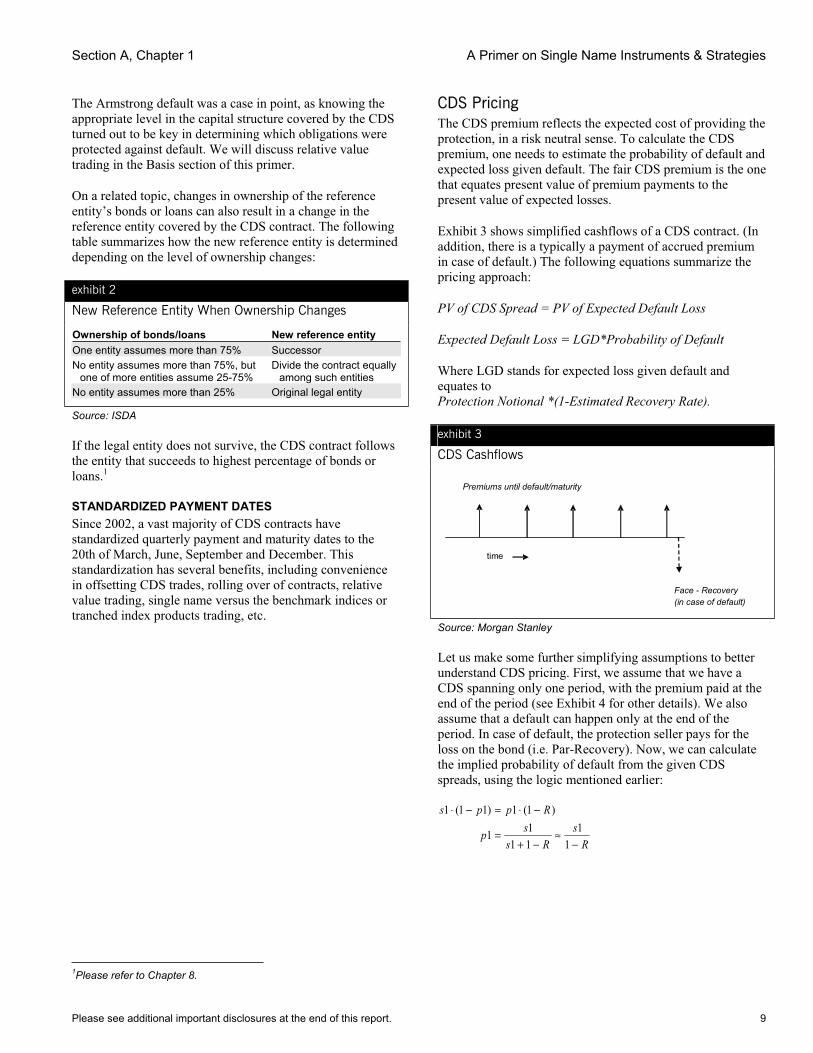
CDS Pricing The CDS premium reflects the expected cost of providing the protection, in a risk neutral sense. To calculate the CDS premium, one needs to estimate the probability of default and expected loss given default. The fair CDS premium is the one that equates present value of premium payments to the present value of expected losses.
Exhibit 3 shows simplified cashflows of a CDS contract. (In addition, there is a typically a payment of accrued premium in case of default.) The following equations summarize the pricing approach:
PV of CDS Spread = PV of Expected Default Loss
Expected Default Loss = LGD*Probability of Default
Where LGD stands for expected loss given default and equates to Protection Notional *(1-Estimated Recovery Rate).
exhibit 3
CDS Cashflows
Premiums until default/maturity
time
Face - Recovery(in case of default)
Source: Morgan Stanley
Let us make some further simplifying assumptions to better understand CDS pricing. First, we assume that we have a CDS spanning only one period, with the premium paid at the end of the period (see Exhibit 4 for other details). We also assume that a default can happen only at the end of the period. In case of default, the protection seller pays for the loss on the bond (i.e. Par-Recovery). Now, we can calculate the implied probability of default from the given CDS spreads, using the logic mentioned earlier:
Rs
Rssp
Rpps
−≈
−+=
−⋅=−⋅
11
1111
)1(1)11(1

Morgan Stanley Credit Derivatives Insights – Handbook of Single Name and Index Strategies
10 Please see additional important disclosures at the end of this report.
exhibit 4
Determining Default Probabilities
Assumptions
s1 CDS spread for single period maturitys2 CDS spread for two period maturityp1 probability of default in the first periodp2 probability of default in the second periodR recovery ratet time periodr riskfree rate
Single Period
s1
1-p1
p1
-(1-R)
Two Period s2
1-p2
s2
1-p1p2
-(1-R)Default
p1
-(1-R)
t
Source: Morgan Stanley
Now, we extend the model to two periods. Similar to one-period calculations, we can equate the present value of CDS spread to expected losses in the case of default to get the implied probability of default in the second period, as shown in the two-period probability tree. The following equation summarizes this calculation:
22 )1(2)11()1(
11)1(
)1()21()11(2
1)11(2
trppR
trpR
trpps
trps
⋅+⋅−⋅−+
⋅+⋅−=
⋅+−⋅−⋅+
⋅+−⋅
PV of Spread PV of Default
Since we know all the variables other than p2, we can calculate it from this equation.
NUMERICAL ILLUSTRATION In Exhibit 5, we have shown a numerical example using the discussed approach to calculate default probabilities, given a CDS curve and fixed recovery rate assumptions.
exhibit 5
Default Probability – Numerical Example
1 Year Spread 0.50%2 Year Spread 1.00% Recovery Rate 40%Risk-free Rate 2% p1 0.83%p2 2.48% PV Default 0.0190PV Premium 0.0190
Note: Calculation assumes annual premium payment. Source: Morgan Stanley
CONTINUOUS TIME IMPLEMENTATIONS Since defaults do not have to happen on payment dates, and premium frequency does not have to match the time steps in the calculation shown above, most commonly used CDS pricing models consider the default process as a continuous time phenomenon, along with discrete numerical techniques to estimate the present value of defaults and premiums. These models are calibrated to the market CDS curve (typically, to get a piecewise constant default intensity function for a given constant recovery rate).
The CDSW function on Bloomberg gives users an option to pick one of the three available numerical implementations of continuous time models. Further details on the three models are available in Bloomberg help.
Section A, Chapter 1 A Primer on Single Name Instruments & Strategies
Please see additional important disclosures at the end of this report. 11
Using these models, we can easily calculate a set of risk-neutral default probabilities from an issuer’s CDS curve. We can then use them to value other debt obligations – including bonds – and to calculate the mark-to-market value of a CDS struck at a price different from the prevailing market price. Additionally we can use these models to convert a running premium to upfront, and vice-versa.
POINTS UPFRONT As we mentioned earlier, default swaps on issuers with high default probabilities typically trade on an upfront plus running basis, rather than on a par spread basis (i.e. quarterly premium, no upfront payment). That is, the protection buyer pays a large part of the premium at the inception of the contract and a lower spread quarterly. For example, instead of paying 2000 bp running the protection buyer would pay 34% upfront and 500 bp running.
Theoretically, the present value of the two premium streams should match when we take default probabilities and timing of cashflows into consideration. However, a higher upfront payment and lower running premium result in better cashflow matching from a hedging perspective, given that the reference entity’s bonds would also be trading at a significant discount to par due to distress.
Given that the protection buyer stops paying quarterly premiums when a default occurs, the equivalent upfront payment should be lower than the simple present value of the running premium difference (1500 bp in our example) at risk-free rates.
The first step for conversion of par spread to upfront is to calculate default probabilities, as we explained in the CDS pricing section. Then using these probabilities we calculate the present value of the par spread (2000 bp in our example), by multiplying the spread with the probability of survival at the time of payment and then discounting back using risk-free zero rates. Now, this present value should equal the present value of upfront and running premiums (34% upfront and 500 bp running in our example), based on the same default probabilities.
A convenient way to do this conversion is to use the CDSW function on Bloomberg. We simply put “Deal Spread” to the running spread and value to the CDS using the par CDS spread. The “Market Value” represents the equivalent upfront payment. We provide additional details on this function in the Useful Bloomberg Functions section of this chapter.
IMPORTANCE OF RECOVERY RATE ASSUMPTION As we discussed earlier, default probabilities and recovery rate are intricately related. That is why the recovery rate assumption can have a significant impact on the mark-to-market of an off-market CDS and hence there exists the possibility of disagreement between two counterparties on the payment required to close such transactions, even when both parties are using identical models.
The bottom line is that to price a credit default swap, we need to have a view on market-implied recovery rates and default probabilities. However, we cannot directly observe these variables in the marketplace. That said, assuming one of the two is fixed, we can estimate the other using on-the-run CDS pricing. Additionally, since bond spreads also capture default risk, we can use bond data to estimate CDS pricing, if it is not available directly in the marketplace.
USEFUL BLOOMBERG FUNCTIONS There are a number of functions provided by Bloomberg for finding CDS levels and analyzing values. MSDU <GO> shows Morgan Stanley’s daily pricing for various credit derivatives. Another function that facilitates searching for the current market premium levels for protection on an issuer is CDSD <GO>. The screen also allows the user to search for available CDS for different entities related to the same issuer. Additionally, one can observe the term structure of CDS in a selected currency and for a selected debt type – senior, subordinated, or other.
WCDS <GO> is another useful screen, where one can scroll down a list of the term structure of CDS by industry sectors.
CDSW <GO> is a default swap calculator, with which we can calculate market value, DV01, cashflows, and other sensitivities of a default swap contract. Potential applications of this tool include calculating delta neutral hedge ratios, marking-to-market, and converting running premium to upfront.
Morgan Stanley Credit Derivatives Insights – Handbook of Single Name and Index Strategies
12 Please see additional important disclosures at the end of this report.
The Basis – CDS vs. Bond Arbitrage For most issuers with liquid bonds trading, one can get a good estimate of the market price of the credit risk, and hence, the trading range for the CDS, if not observable directly from the market. This brings us to the subject of basis between an issuer’s bonds and credit default swap, given that we can estimate the price of credit risk from both.
In our discussion, we have deliberately compared CDS levels to bond spreads above Libor, and not Treasuries. A CDS protection buyer and seller inadvertently takes counterparty risk to the banking system. This risk is captured by the difference between Libor and Treasury curves. As such, we tend to treat LIBOR as the risk-free rate throughout our research.
Conceptually, the CDS premium should equate to spread over LIBOR for the issuer’s floating rate note trading at par, and represents the compensation for the default risk. While not all issuers have floating-rate debt outstanding, one can interpret this amount by calculating the zero volatility OAS or Z-spread (defined on the next page) on the issuer’s fixed rate bonds, assuming the bonds are trading at par. If, however, the bonds are trading at a discount or premium, one needs to make some adjustments to determine the default risk premium.
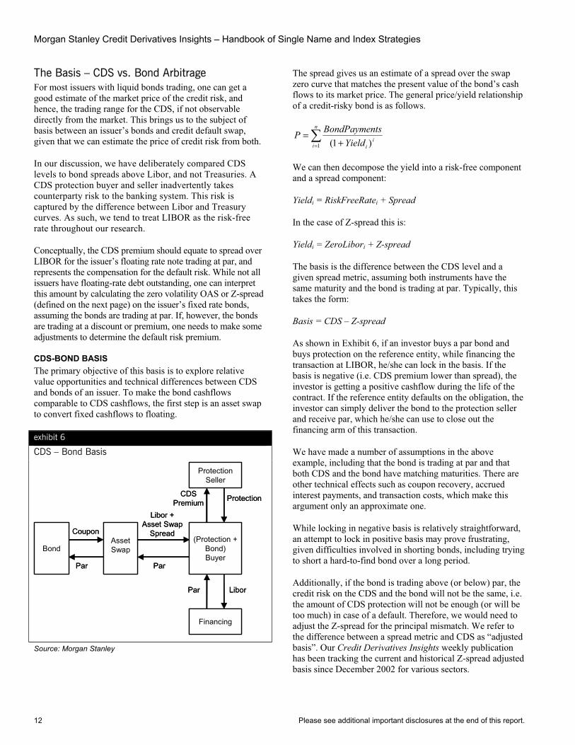
CDS-BOND BASIS The primary objective of this basis is to explore relative value opportunities and technical differences between CDS and bonds of an issuer. To make the bond cashflows comparable to CDS cashflows, the first step is an asset swap to convert fixed cashflows to floating.
exhibit 6
CDS – Bond Basis
Bond
CouponAssetSwap
Par
(Protection + Bond)Buyer
Libor +Asset Swap
Spread
Par
ProtectionSeller
Financing
Par
CDSPremium
Libor
Protection
Bond
CouponAssetSwap
Par
(Protection + Bond)Buyer
Libor +Asset Swap
Spread
Par
ProtectionSeller
Financing
Par
CDSPremium
Libor
Protection
Source: Morgan Stanley
The spread gives us an estimate of a spread over the swap zero curve that matches the present value of the bond’s cash flows to its market price. The general price/yield relationship of a credit-risky bond is as follows.
= +=
n
ii
iYieldtsBondPaymenP
1 )1(
We can then decompose the yield into a risk-free component and a spread component:
Yieldi = RiskFreeRatei + Spread
In the case of Z-spread this is:
Yieldi = ZeroLibori + Z-spread
The basis is the difference between the CDS level and a given spread metric, assuming both instruments have the same maturity and the bond is trading at par. Typically, this takes the form:
Basis = CDS – Z-spread
As shown in Exhibit 6, if an investor buys a par bond and buys protection on the reference entity, while financing the transaction at LIBOR, he/she can lock in the basis. If the basis is negative (i.e. CDS premium lower than spread), the investor is getting a positive cashflow during the life of the contract. If the reference entity defaults on the obligation, the investor can simply deliver the bond to the protection seller and receive par, which he/she can use to close out the financing arm of this transaction.
We have made a number of assumptions in the above example, including that the bond is trading at par and that both CDS and the bond have matching maturities. There are other technical effects such as coupon recovery, accrued interest payments, and transaction costs, which make this argument only an approximate one.
While locking in negative basis is relatively straightforward, an attempt to lock in positive basis may prove frustrating, given difficulties involved in shorting bonds, including trying to short a hard-to-find bond over a long period.
Additionally, if the bond is trading above (or below) par, the credit risk on the CDS and the bond will not be the same, i.e. the amount of CDS protection will not be enough (or will be too much) in case of a default. Therefore, we would need to adjust the Z-spread for the principal mismatch. We refer to the difference between a spread metric and CDS as “adjusted basis”. Our Credit Derivatives Insights weekly publication has been tracking the current and historical Z-spread adjusted basis since December 2002 for various sectors.

Section A, Chapter 1 A Primer on Single Name Instruments & Strategies
Please see additional important disclosures at the end of this report. 13
CURVE ADJUSTMENTS TO THE BASIS Having adjusted the basis measure for maturity gaps between the bond and the CDS, as well as for the bond’s market price being at a premium/discount to par, we can further sharpen our relative value measure by using the full term structure of CDS, which is now possible given the increased market liquidity across the curve.
For this adjustment, instead of using a constant CDS premium above the swap zero curve, we can use a spread that varies with the timing of the cashflows, in accordance with the term structure of default swaps. The first step is to determine probabilities of survival for various cashflow dates using the CDS curve. The next step is to calculate present value of cashflows, using survival probabilities for coupon and principal cashflows and default probabilities for the recovery value in case of default. Thus, we get a price for the bond that is consistent with the full CDS curve and current interest rate environment. The following equation summarizes the above calculation:
PRppp)1()1(
where
Pricer
RpCFi
ti
iiii
=+
.+−.
)1()1(
where
Pricer
RCFi
ti
iiii
=+
.+−.
)1()1(
where
Pricer
RCFi
ti
iiii
=+
.+−.
)1()1(
where
Pricer
CFi
ti
iiii
)( , Csfp ii= )( , Csfp ii= )( , Csfp ii= )( , Csfp ii=
=+
.+−.
)( , CsgP ii= )( , Cs ii= )( , Cs ii= )( , Cs ii=
,
PRppp)1()1(
where
Pricer
RpCFi
ti
iiii
=+
.+−.
)1()1(
where
Pricer
RCFi
ti
iiii
=+
.+−.
)1()1(
where
Pricer
RCFi
ti
iiii
=+
.+−.
)1()1(
where
Pricer
CFi
ti
iiii
)( , Csfp ii= )( , Csfp ii= )( , Csfp ii= )( , Csfp ii= )( , Csfp ii= )( , Csfp ii= )( , Csfp ii= )( , Csfp ii=
=+
.+−.
)( , CsgP ii= )( , Cs ii= )( , Cs ii= )( , Cs ii=
,
CFi represents the bond’s cashflows (coupon as well as principal), R is the recovery rate assumption, and ri is the discount rate (boot-strapped from the swap curve). The default probabilities (pi and Pi) above are determined from the CDS curve (si) and the constant C. The factor (1- pi)represents the probability of survival up to i while Pirepresents the incremental probability of default during period i. The constant C represents a parallel shift in the CDS curve, and by changing it we can match the present value of cashflows to the market price. For details on how to calculate default probabilities from spread, refer to the CDS pricing section of this primer.
Once we have the implied CDS curve from the bond price, we can calculate another measure of basis – this time between the actual default swap and the implied default swap spread. We call this measure the curve-adjusted or fair value basis, and have been tracking it in our publications since December 2004.
While the Curve-Adjusted basis indicates the true relative value taking into account the full CDS curve, the Z-spread basis captures the carry on the basis trade between the bond and the CDS (assuming that the bond is trading at par). When both the carry and the fair value basis measures point in the same direction and the gap is large enough to cover transaction costs, the relative value trade may be compelling, technical factors aside.
REASONS FOR NON-TRIVIAL BASIS There are several reasons for the existence of a basis between bonds and CDS. We discuss the salient ones here:
• Maturity Differences. Maturities of an issuer’s CDS seldom exactly match maturities of its bonds. Consequently, in most cases, one has to interpolate or extrapolate the CDS curve to estimate the default swap premium directly comparable to the bond spreads.
• Bond Price. In case of a default, the CDS pays the difference between par and recovery rate, implying that the protection would be insufficient for bonds trading at premium and too much for bonds trading at discount.
• Difficulty in Shorting Bonds. To arbitrage away positive basis, one needs to short the bond (and write protection in the form of CDS), which is not always easy, especially for an extended period of time.
• Bond Covenants. Bonds may have covenants, such as put/call options, tender with make-whole, coupon step-ups, change of control provisions, equity clawbacks, etc., which would affect their spread. This would distort the basis as CDS assumes a generic reference obligation and, in case of default, a protection buyer would look for a bond with the least attractive covenants for a physical settlement, given the embedded cheapest-to-deliver option.
• Restructuring Feature. Restructuring clauses in CDS contracts often create economic differences between taking credit risk in the form of CDS versus bonds (see the section on restructuring for more details). This would also tend to distort the basis.
• Technical Factors. Prevailing supply/demand imbalances in the marketplace between bonds and CDS also impact the basis.
• Liquidity. Liquidity may result in temporary misalignments between bonds and CDS, giving rise to negative or positive basis.
• Transaction Costs. To arbitrage the basis, one has to incur transaction costs associated with the bid-ask spread on bonds and CDS. Thus arbitrageurs have an incentive to trade only if the basis exceeds this band of transaction costs.
• Interest Rate Exposure. In case of a default, the cash flows of a CDS and the bond swapped into floating rate do not match. This is due to the reason that the interest rate swap does not disappear with default on the bond. Consequently, we have to incur additional transaction costs and bear the market risk of the interest rate swap.
Morgan Stanley Credit Derivatives Insights – Handbook of Single Name and Index Strategies
14 Please see additional important disclosures at the end of this report.
Implications of Restructuring as a Credit Event Earlier we briefly mentioned restructuring as one of the credit events covered by some default swaps. In this section, we further elaborate on this contract feature and analyze its potential implications on CDS pricing. Restructuring of a debt obligation refers to one or more of the following actions:
• A reduction in interest rate, amount payable or accrual
• A reduction in amount of principal or premium payable
• Postponement or deferral of interest or principal payments
• Change in ranking
• Change in currency to a “non permitted” currency
In order for the actions above to constitute a credit event, such actions must result, directly or indirectly, from a deterioration in the creditworthiness or financial condition of the reference entity.
The evolution of various restructuring options, which we will discuss shortly, directly reflects the motivation to improve the matching of economics behind protection selling and bond purchases. Not surprisingly, losses suffered by many protection sellers and buyers during various actual restructuring events were the main driver behind this evolution.
The most vibrant memory that comes to mind in this regard is that of Conseco, which restructured some of its debt. The restructuring did not materially affect the company’s bonds with comparable maturities; however, the outcome for the CDS protection seller was significantly worse, highlighting the dramatically different economics for default swaps and bonds. This motivated Modified-R changes (see below for details).
Current ISDA agreement offers four types of restructuring options that affect the protection buyer’s privileges:
Full Restructuring (Old-R) Under this definition, a bond of any maturity is deliverable after a restructuring credit event by the reference entity. There are no limitations on maturity of deliverable obligations (up to 30 years) and no multiple holder requirement on the restructured obligation (see more details on this point in the Mod-R section).
No Restructuring (No-R) This definition is typical in case of high yield CDS in the US and completely excludes restructuring as a credit event that could trigger the CDS. This feature gives a protection seller significant advantages over a bondholder. We will discuss the valuation implications shortly.
Modified Restructuring (Mod-R) Modified restructuring has become a market standard in the US for CDS on investment grade credits. Under this
definition, the most material change is the limitation on the maturity of deliverable obligations. In case of a restructuring credit event, the protection buyer must deliver obligations with a maturity date that is the earlier of a) 30 months following the restructuring, or b) the latest final maturity date of any restructured bond or loan, but not shorter than the CDS contract. The argument for this limitation on the universe of potentially deliverable bonds is to prevent certain abuses of the restructuring feature. Since longer maturity bonds are more likely to trade at a significant discount to par due to interest rate moves even when there are no changes in the creditworthiness of the issuer, this provision limits gains to a protection buyer in cases where restructuring does not have an economic impact on the bond by excluding these obligations from the list of deliverables.
Another important feature of Mod-R is related to limitations on debt obligations that can trigger a restructuring credit event. Under Mod-R, these obligations have to be held by more than three non-affiliated holders in order to qualify for a restructuring event. Consequently, for example, a bilateral agreement between a bank and the issuer to extend the maturity of an outstanding loan does not trigger the default swap.
Modified-Modified-Restructuring (Mod-Mod-R) Under this definition, which is more popular in Europe for both investment grade and high yield, the main difference from Mod-R is that the protection buyer can deliver a deliverable obligation with maturity up to 60 months after restructuring (in the case of the restructured bond or loan) and 30 months in the case of all other deliverable obligations. The goal of this improvement over mod-R is to allow for a wider range of deliverables, as in certain cases, the 30-month restriction may prove too limiting.
PRICING IMPLICATIONS OF RESTRUCTURING To understand the economic implications of these restructuring definitions, we assume that we have a fully hedged position combining a deliverable bond and a CDS. Now, if the CDS does not cover restructuring events, our hedge would not work perfectly in case of a restructuring of debt without an eventual default. On the other hand, if the CDS covers restructuring, it would protect us from any losses related to such an event. Furthermore, if the restructured obligation is not the obligation we own, there is a potential gain, even when there is no direct adverse impact on our position. Thus, we would be willing pay more for a CDS with restructuring than for a CDS without restructuring.
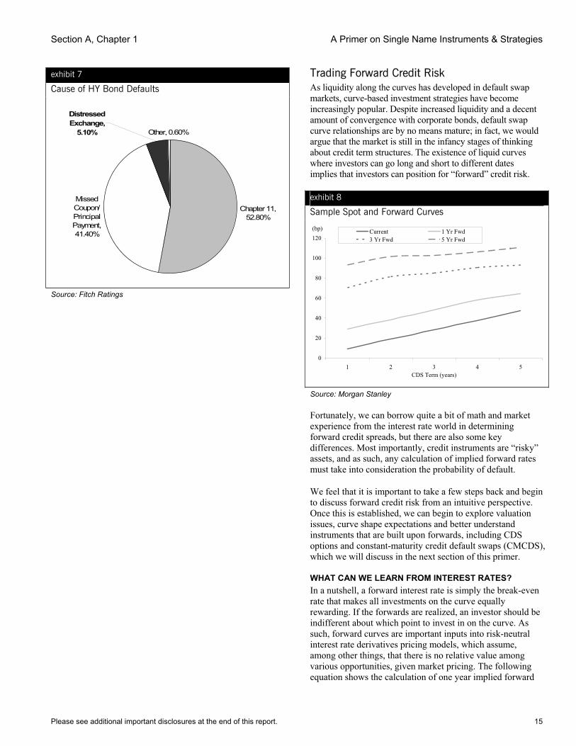
To get a sense of the magnitude of the impact of restructuring on CDS spreads, we looked at the US high yield market, where restructuring is more frequent. About 5% of total high yield defaults in the US result in some kind of restructuring (see Exhibit 7), implying a material difference between R and No-R contracts.
Section A, Chapter 1 A Primer on Single Name Instruments & Strategies
Please see additional important disclosures at the end of this report. 15
exhibit 7
Cause of HY Bond Defaults
Chapter 11, 52.80%
Missed Coupon/ Principal Payment, 41.40%
Other, 0.60%
Distressed Exchange,
5.10%
Source: Fitch Ratings
Trading Forward Credit Risk As liquidity along the curves has developed in default swap markets, curve-based investment strategies have become increasingly popular. Despite increased liquidity and a decent amount of convergence with corporate bonds, default swap curve relationships are by no means mature; in fact, we would argue that the market is still in the infancy stages of thinking about credit term structures. The existence of liquid curves where investors can go long and short to different dates implies that investors can position for “forward” credit risk.
exhibit 8
Sample Spot and Forward Curves
(bp)
0
20
40
60
80
100
120
1 2 3 4 5CDS Term (years)
Current 1 Yr Fwd3 Yr Fwd 5 Yr Fwd
Source: Morgan Stanley
Fortunately, we can borrow quite a bit of math and market experience from the interest rate world in determining forward credit spreads, but there are also some key differences. Most importantly, credit instruments are “risky” assets, and as such, any calculation of implied forward rates must take into consideration the probability of default.
We feel that it is important to take a few steps back and begin to discuss forward credit risk from an intuitive perspective. Once this is established, we can begin to explore valuation issues, curve shape expectations and better understand instruments that are built upon forwards, including CDS options and constant-maturity credit default swaps (CMCDS), which we will discuss in the next section of this primer.
WHAT CAN WE LEARN FROM INTEREST RATES? In a nutshell, a forward interest rate is simply the break-even rate that makes all investments on the curve equally rewarding. If the forwards are realized, an investor should be indifferent about which point to invest in on the curve. As such, forward curves are important inputs into risk-neutral interest rate derivatives pricing models, which assume, among other things, that there is no relative value among various opportunities, given market pricing. The following equation shows the calculation of one year implied forward
Morgan Stanley Credit Derivatives Insights – Handbook of Single Name and Index Strategies
16 Please see additional important disclosures at the end of this report.
rate starting at the end of year 1, F1-2, given the one year spot rate S1 and the two year spot rate S2:
F1-2=(1+S2)2/(1+S1) - 1
WHAT IS DIFFERENT IN CREDIT? – IMPLIED FORWARD CDS PREMIUMS On the surface, the same math and relationships used in interest rates should hold for credit, but a key difference is that credit is “risky.” As such, we have to make some adjustments to address the issue that if the reference entity defaults, the protection seller is not entitled to any future premiums and has to pay the difference between par and recovery value. From a set of CDS levels extending up to the end of the intended forward default swap, we can determine the forward spread using the following logic: A long position in a two-year CDS starting now is equivalent to a combination of a long position in a one-year CDS starting now and a long position in a one-year CDS starting one year from now.
The first step toward calculating implied forward rates is to calculate default probabilities for each payment period. To simplify, let us assume that we have two default swap contracts, CDS1 and CDS2, maturing at the end of year 1 and 2, respectively, with annual spread payments. Now we can determine the implied probability of default at the end of year 1 from CDS1, given a recovery rate. Similarly, given the probability of default in year 1 and CDS2 spread level, we can calculate the probability of default in year 2, given the reference entity does not default in year 1. Thus, we can impute default probabilities for each period from a whole credit curve. For more details, refer to the CDS Pricing section.
The combination of CDS1 and a forward default swap, which starts at the end of year 1, replicates CDS2. Therefore, by equating the two cashflow streams, we can determine the implied forward default swap level.
The following equations summarize the calculation of forward CDS rates (using the same notation as we used in the CDS Pricing section):
= −
−−
=
−
−+
⋅=
−+
⋅=
=+
T
itt
Ti
TitTi
T
tt
T
TtT
TTtt
RF
FDFFWDPV
RS
SDFCDSPV
whereCDSPVFWDPVCDSPV
11
)(
11
)(
)()()(
1
The first equation represents replication of a CDS maturity at T with a CDS of term t and a forward-starting CDS that starts at t and ends at T. DFt represent discount factors and can be calculated using the swap curve.
exhibit 9
Forward Trading – Hypothetical Example
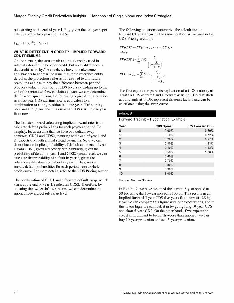
Year CDS Spread 5 Yr Forward CDS0 0.00% 0.50%1 0.10% 0.72%2 0.20% 0.97%3 0.30% 1.23%4 0.40% 1.53%5 0.50% 1.88%6 0.60%7 0.70% 8 0.80%9 0.90% 10 1.00%
Source: Morgan Stanley
In Exhibit 9, we have assumed the current 5-year spread at 50 bp, while the 10-year spread is 100 bp. This results in an implied forward 5-year CDS five years from now of 188 bp. Now we can compare this figure with our expectations, and if this is too high, we can lock it in by going long 10-year CDS and short 5-year CDS. On the other hand, if we expect the credit environment to be much worse than implied, we can buy 10-year protection and sell 5-year protection.
Section A, Chapter 1 A Primer on Single Name Instruments & Strategies
Please see additional important disclosures at the end of this report. 17
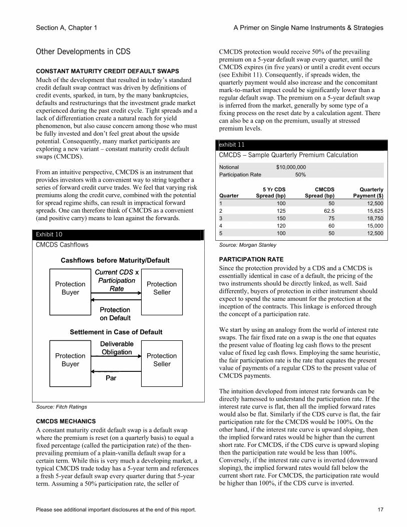
Other Developments in CDS
CONSTANT MATURITY CREDIT DEFAULT SWAPS Much of the development that resulted in today’s standard credit default swap contract was driven by definitions of credit events, sparked, in turn, by the many bankruptcies, defaults and restructurings that the investment grade market experienced during the past credit cycle. Tight spreads and a lack of differentiation create a natural reach for yield phenomenon, but also cause concern among those who must be fully invested and don’t feel great about the upside potential. Consequently, many market participants are exploring a new variant – constant maturity credit default swaps (CMCDS).
From an intuitive perspective, CMCDS is an instrument that provides investors with a convenient way to string together a series of forward credit curve trades. We feel that varying risk premiums along the credit curve, combined with the potential for spread regime shifts, can result in impractical forward spreads. One can therefore think of CMCDS as a convenient (and positive carry) means to lean against the forwards.
Exhibit 10
CMCDS Cashflows
BuyerProtection
Protection Seller
Current CDS xParticipation
Rate
Protection on Default
Cashflows before Maturity/Default
Protection Buyer
Protection Seller
Deliverable Obligation
Par
Settlement in Case of Default
Protection Buyer
Protection Seller
Current CDS xParticipation
Rate
Protection on Default
Protection Buyer
Protection Seller
Deliverable Obligation
Par
Source: Fitch Ratings
CMCDS MECHANICS A constant maturity credit default swap is a default swap where the premium is reset (on a quarterly basis) to equal a fixed percentage (called the participation rate) of the then-prevailing premium of a plain-vanilla default swap for a certain term. While this is very much a developing market, a typical CMCDS trade today has a 5-year term and references a fresh 5-year default swap every quarter during that 5-year term. Assuming a 50% participation rate, the seller of
CMCDS protection would receive 50% of the prevailing premium on a 5-year default swap every quarter, until the CMCDS expires (in five years) or until a credit event occurs (see Exhibit 11). Consequently, if spreads widen, the quarterly payment would also increase and the concomitant mark-to-market impact could be significantly lower than a regular default swap. The premium on a 5-year default swap is inferred from the market, generally by some type of a fixing process on the reset date by a calculation agent. There can also be a cap on the premium, usually at stressed premium levels.
exhibit 11
CMCDS – Sample Quarterly Premium Calculation
Notional $10,000,000 Participation Rate 50%
Quarter 5 Yr CDS
Spread (bp) CMCDS
Spread (bp)Quarterly
Payment ($)1 100 50 12,5002 125 62.5 15,6253 150 75 18,7504 120 60 15,0005 100 50 12,500
Source: Morgan Stanley
PARTICIPATION RATE Since the protection provided by a CDS and a CMCDS is essentially identical in case of a default, the pricing of the two instruments should be directly linked, as well. Said differently, buyers of protection in either instrument should expect to spend the same amount for the protection at the inception of the contracts. This linkage is enforced through the concept of a participation rate.
We start by using an analogy from the world of interest rate swaps. The fair fixed rate on a swap is the one that equates the present value of floating leg cash flows to the present value of fixed leg cash flows. Employing the same heuristic, the fair participation rate is the rate that equates the present value of payments of a regular CDS to the present value of CMCDS payments.
The intuition developed from interest rate forwards can be directly harnessed to understand the participation rate. If the interest rate curve is flat, then all the implied forward rates would also be flat. Similarly if the CDS curve is flat, the fair participation rate for the CMCDS would be 100%. On the other hand, if the interest rate curve is upward sloping, then the implied forward rates would be higher than the current short rate. For CMCDS, if the CDS curve is upward sloping then the participation rate would be less than 100%. Conversely, if the interest rate curve is inverted (downward sloping), the implied forward rates would fall below the current short rate. For CMCDS, the participation rate would be higher than 100%, if the CDS curve is inverted.
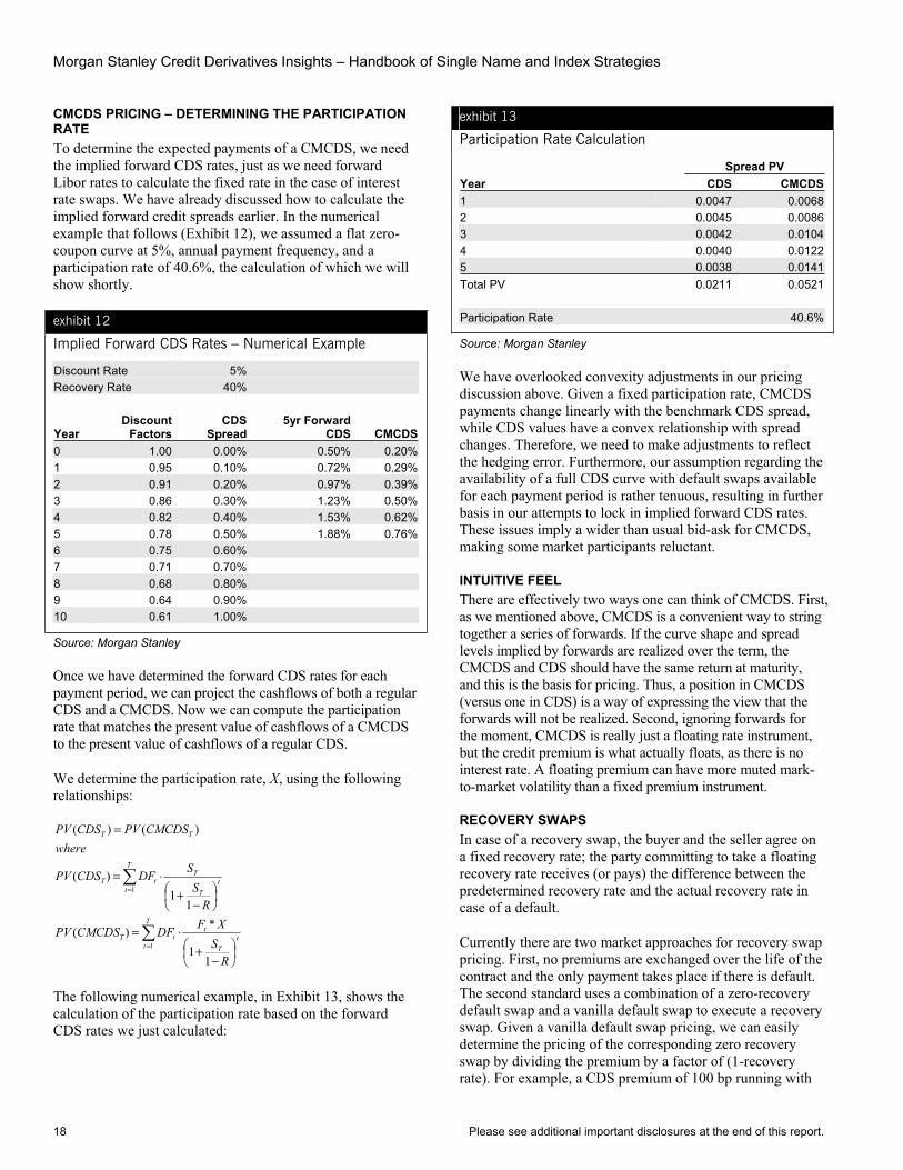
Morgan Stanley Credit Derivatives Insights – Handbook of Single Name and Index Strategies
18 Please see additional important disclosures at the end of this report.
CMCDS PRICING – DETERMINING THE PARTICIPATION RATE To determine the expected payments of a CMCDS, we need the implied forward CDS rates, just as we need forward Libor rates to calculate the fixed rate in the case of interest rate swaps. We have already discussed how to calculate the implied forward credit spreads earlier. In the numerical example that follows (Exhibit 12), we assumed a flat zero-coupon curve at 5%, annual payment frequency, and a participation rate of 40.6%, the calculation of which we will show shortly.
exhibit 12
Implied Forward CDS Rates – Numerical Example
Discount Rate 5%Recovery Rate 40%
YearDiscount
Factors CDS
Spread5yr Forward
CDS CMCDS0 1.00 0.00% 0.50% 0.20%1 0.95 0.10% 0.72% 0.29%2 0.91 0.20% 0.97% 0.39%3 0.86 0.30% 1.23% 0.50%4 0.82 0.40% 1.53% 0.62%5 0.78 0.50% 1.88% 0.76%6 0.75 0.60%7 0.71 0.70% 8 0.68 0.80%9 0.64 0.90% 10 0.61 1.00%
Source: Morgan Stanley
Once we have determined the forward CDS rates for each payment period, we can project the cashflows of both a regular CDS and a CMCDS. Now we can compute the participation rate that matches the present value of cashflows of a CMCDS to the present value of cashflows of a regular CDS.
We determine the participation rate, X, using the following relationships:
=
=
−+
⋅=
−+
⋅=
=
T
tt
T
ttT
T
tt
T
TtT
TT
RS
XFDFCMCDSPV
RS
SDFCDSPV
whereCMCDSPVCDSPV
1
1
11
*)(
11
)(
)()(
The following numerical example, in Exhibit 13, shows the calculation of the participation rate based on the forward CDS rates we just calculated:
exhibit 13
Participation Rate Calculation
Spread PV Year CDS CMCDS1 0.0047 0.00682 0.0045 0.00863 0.0042 0.01044 0.0040 0.01225 0.0038 0.0141Total PV 0.0211 0.0521
Participation Rate 40.6%
Source: Morgan Stanley
We have overlooked convexity adjustments in our pricing discussion above. Given a fixed participation rate, CMCDS payments change linearly with the benchmark CDS spread, while CDS values have a convex relationship with spread changes. Therefore, we need to make adjustments to reflect the hedging error. Furthermore, our assumption regarding the availability of a full CDS curve with default swaps available for each payment period is rather tenuous, resulting in further basis in our attempts to lock in implied forward CDS rates. These issues imply a wider than usual bid-ask for CMCDS, making some market participants reluctant.
INTUITIVE FEEL There are effectively two ways one can think of CMCDS. First, as we mentioned above, CMCDS is a convenient way to string together a series of forwards. If the curve shape and spread levels implied by forwards are realized over the term, the CMCDS and CDS should have the same return at maturity, and this is the basis for pricing. Thus, a position in CMCDS (versus one in CDS) is a way of expressing the view that the forwards will not be realized. Second, ignoring forwards for the moment, CMCDS is really just a floating rate instrument, but the credit premium is what actually floats, as there is no interest rate. A floating premium can have more muted mark-to-market volatility than a fixed premium instrument.
RECOVERY SWAPS In case of a recovery swap, the buyer and the seller agree on a fixed recovery rate; the party committing to take a floating recovery rate receives (or pays) the difference between the predetermined recovery rate and the actual recovery rate in case of a default.
Currently there are two market approaches for recovery swap pricing. First, no premiums are exchanged over the life of the contract and the only payment takes place if there is default. The second standard uses a combination of a zero-recovery default swap and a vanilla default swap to execute a recovery swap. Given a vanilla default swap pricing, we can easily determine the pricing of the corresponding zero recovery swap by dividing the premium by a factor of (1-recovery rate). For example, a CDS premium of 100 bp running with

Section A, Chapter 1 A Primer on Single Name Instruments & Strategies
Please see additional important disclosures at the end of this report. 19
40% recovery translates to 166.7 bp with 0% recovery. From our discussions, it appears that the market is leaning toward the former for pricing recovery swaps.2
CANCELABLE CDS A cancelable default swap (also known as a callable default swap) is a credit default swap where the buyer of protection has the right to cancel the protection after a non-call period. The motivation behind cancelable CDS is an effort to hedge loans or bonds with uncertain maturity, such as prepayable bank loans, convertible/callable bonds, etc. For example, we can hedge a callable bond by buying cancelable protection, as we can cancel the CDS if the bond is called away. The motivation for the protection seller is the opportunity to make some additional spread, to compensate him/her for being short the option. A short cancelable CDS position (long protection) is implicitly bullish on spread, since the cancelable option becomes more valuable as spread declines. In other words, as spreads tighten, the long protection position would have a negative mark-to-market, and the option to cancel this contract would now be in-the-money.
SPREAD OPTIONS Spread options provide a convenient way to hedge uncertain credit risk exposure and to position for volatility changes. Options to buy or sell protection on individual credits as well as diversified indices are now available in the marketplace, albeit liquidity may vary considerably depending on the credit.
Options on default swaps work in a fashion similar to the over-the-counter (OTC) options with a few subtle differences. Upon exercise of an option of CDS, the option buyer is enters a long or short default swap position, depending on the option.
2Please refer to Chapter 4.
TYPES OF OPTIONS There are two types of options on credit default swaps, as explained below:
• Option to buy protection (put/payer). Upon exercise, the option holder enters into a long protection position on the underlying reference entity.
• Option to sell protection (call/receiver). Upon exercise, the option holder enters into a short protection position on the underlying reference entity.
Option premium is typically quoted on an upfront basis. The strike is typically European in nature, i.e. the option can only be exercised on the expiration date. Upon exercise, the two parties enter into a default swap and the option seller makes an upfront payment reflecting the difference between the strike and the current CDS level, just as one does while entering into an off-market CDS transaction. Options with maturities up to one year are usually available, with the near term options typically being most liquid. The maturity dates usually coincide with the standard default swap payment dates.
It is noteworthy that single name spread options typically do not provide protection against default during their life. If a default occurs during this period, the option is simply knocked out. However, spread options on indices tend to trade without the knock-out feature, i.e. they provide protection during the option’s life and the buyer has the right to exercise on defaults at expiration.
The default swap option premium depends on the current CDS level, the strike spread, Libor interest rate curve, volatility of spread, and maturity dates of the option and the CDS. The payoff function of an option to buy protection looks similar to an equity call payoff, while it resembles an equity put option for an option to sell protection.

Morgan Stanley Credit Derivatives Insights – Handbook of Single Name and Index Strategies
20 Please see additional important disclosures at the end of this report.
Chapter 2
Understanding Synthetic Structured Finance – First Steps
The powerful credit derivatives force that began well over 10 years ago in the emerging markets sovereign debt arena and over time introduced a secular shift in the corporate credit markets has now reshaped the structured finance markets as well. In both corporate and emerging markets credit, it has paved the way for the emergence of innovative ways of transferring credit risk, implementing hedging strategies and expanding investment opportunities for a wide range of market participants. In our view, it is too early to tell whether the derivatives culture will be as welcomed in structured finance as it was in the other two markets, but investor demand, the instruments and standardization discussions have certainly progressed enough to make synthetics more than just a niche within the structured finance world.
By our measures, the synthetic structured finance market is at least five years old, but significant recent developments have served as important first steps in what will likely be a multi-year development process. From a research perspective, we begin describing our first thoughts on this market with a brief review of the original credit derivatives markets, which provide an important benchmark for the amount of development and the tests that were necessary for derivative instruments to mature in the sovereign emerging and corporate credit markets.
A BRIEF HISTORY OF THE CREDIT DEFAULT SWAP1
Within the corporate credit and sovereign emerging markets, credit default swap contracts experienced many important tests over the past 10 years that both shaped the contract and eventually provided the motivation for standardization. Indonesia’s debt restructuring in 1997 encouraged working groups to address standardization, but it was not until 1999 that the International Swaps and Derivatives Association (ISDA) published the first market standard terms. Between 2000 and 2003, numerous credit events had significant impacts on the standardization process – including Conseco and Xerox (restructuring), Armstrong (reference entity disagreements), Railtrack (deliverability of convertible bonds), and the trio of Enron, Argentina and Parmalat (volume of outstanding contracts).
Today’s standard credit derivatives definitions (published by ISDA in 2003) reflect lessons market participants learned during this period, and have encouraged explosive growth in both single-name derivatives and in structured credit. Commercial banks, which lend directly to corporations, continue to be among the biggest and most natural buyers of protection in the market. Other significant buyers of protection include hedge funds, and corporates themselves. Estimates of the global outstanding single-name credit default swaps
1Please refer to Chapter 1.
(Exhibit 1) by the Bank for International Settlements2
demonstrate the imposing size the credit derivatives market has now achieved (about $11 trillion notional).
SYNTHETIC STRUCTURED FINANCE In the initial few years of their introduction when there was no “street standard”, the corporate credit default swap market used to be small and fragmented with limited liquidity, wide bid-offer spreads and a narrow base of market participants. However, with the development of standardized contract terms and documentation, the corporate CDS market has quickly evolved into the force that we know today. While market participants can certainly take comfort in knowing that credit default swap contracts referencing sovereign and corporate entities went through a 10-year growing-up process, we argue that issues related to structured finance securities are different along almost every dimension, as are drivers of demand and the natural buyers and sellers.
Structured finance (SF) securities3 have been predominantly a long-only cash market, with limited opportunities for implementing sophisticated hedging or long/short strategies, thanks to the many unique and complex characteristics of SF securities. While CDS on SF securities have been in vogue for some years, mainly in the context of synthetic CDOs, the market for single-asset referencing SF CDS has been fairly limited. The absence of standardized documentation and a commonly accepted set of contract terms hampered the growth of a broader SF CDS market. With the publication of a standard confirmation by the ISDA for CDS designed for RMBS and CMBS reference obligations on June 21, 2005, standardization of documentation appears to be well on track.
As we will describe in more detail throughout this chapter, structured finance instruments have unique characteristics that motivate a different set of credit events and settlement mechanics from a standard default swap contract. These characteristics include available funds caps, payment-in-kind options, unscheduled amortizations, de-levering and principal writedowns, to name a few. In fact, the complexity of such instruments motivated many early users of derivatives to focus on total-return swaps, where cash flows and price movements are passed on directly from one party to the other. But with demand from structured vehicles (CDOs) combining with the recent advances in standardization (2005 ISDA definitions), we expect there to be quite a bit of focus on credit default swaps linked to structured finance instruments.
2See “OTC derivatives market activity in the first half of 2005,” Bank for International Settlements, November 2005. 3We categorize asset-backed securities (ABS), residential mortgage-backed securities (RMBS), commercial mortgage-backed securities (CMBS) and securities issued by collateralized debt obligations (CDO) vehicles under the broad term of structured finance securities.
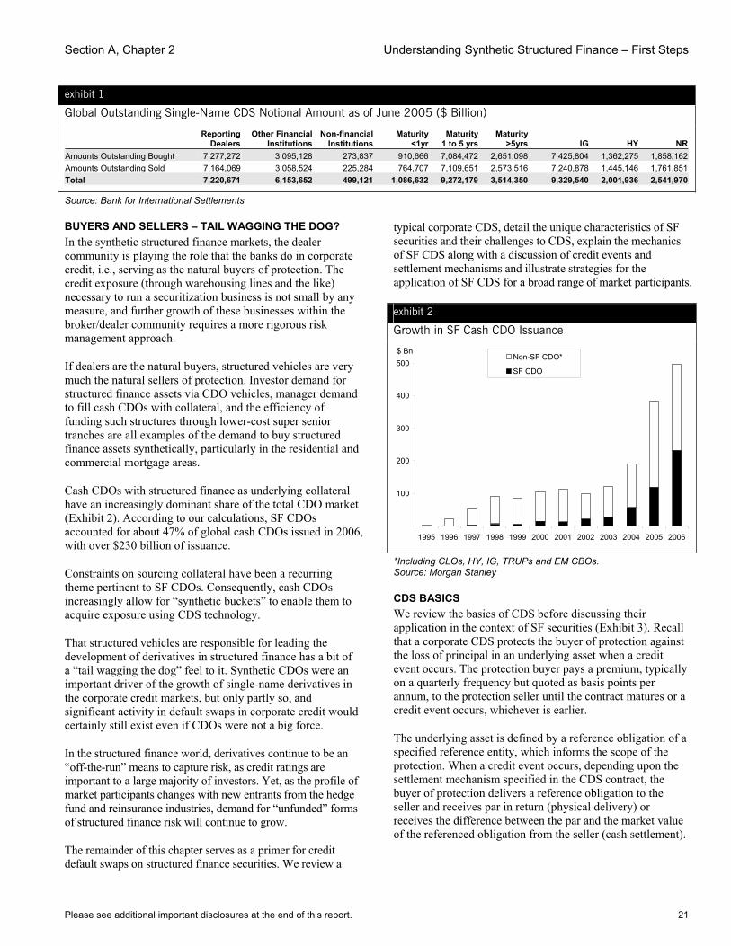
Section A, Chapter 2 Understanding Synthetic Structured Finance – First Steps
Please see additional important disclosures at the end of this report. 21
exhibit 1
Global Outstanding Single-Name CDS Notional Amount as of June 2005 ($ Billion)
Reporting Dealers
Other Financial Institutions
Non-financialInstitutions
Maturity <1yr
Maturity 1 to 5 yrs
Maturity >5yrs IG HY NR
Amounts Outstanding Bought 7,277,272 3,095,128 273,837 910,666 7,084,472 2,651,098 7,425,804 1,362,275 1,858,162Amounts Outstanding Sold 7,164,069 3,058,524 225,284 764,707 7,109,651 2,573,516 7,240,878 1,445,146 1,761,851Total 7,220,671 6,153,652 499,121 1,086,632 9,272,179 3,514,350 9,329,540 2,001,936 2,541,970
Source: Bank for International Settlements
BUYERS AND SELLERS – TAIL WAGGING THE DOG? In the synthetic structured finance markets, the dealer community is playing the role that the banks do in corporate credit, i.e., serving as the natural buyers of protection. The credit exposure (through warehousing lines and the like) necessary to run a securitization business is not small by any measure, and further growth of these businesses within the broker/dealer community requires a more rigorous risk management approach.
If dealers are the natural buyers, structured vehicles are very much the natural sellers of protection. Investor demand for structured finance assets via CDO vehicles, manager demand to fill cash CDOs with collateral, and the efficiency of funding such structures through lower-cost super senior tranches are all examples of the demand to buy structured finance assets synthetically, particularly in the residential and commercial mortgage areas.
Cash CDOs with structured finance as underlying collateral have an increasingly dominant share of the total CDO market (Exhibit 2). According to our calculations, SF CDOs accounted for about 47% of global cash CDOs issued in 2006, with over $230 billion of issuance.
Constraints on sourcing collateral have been a recurring theme pertinent to SF CDOs. Consequently, cash CDOs increasingly allow for “synthetic buckets” to enable them to acquire exposure using CDS technology.
That structured vehicles are responsible for leading the development of derivatives in structured finance has a bit of a “tail wagging the dog” feel to it. Synthetic CDOs were an important driver of the growth of single-name derivatives in the corporate credit markets, but only partly so, and significant activity in default swaps in corporate credit would certainly still exist even if CDOs were not a big force.
In the structured finance world, derivatives continue to be an “off-the-run” means to capture risk, as credit ratings are important to a large majority of investors. Yet, as the profile of market participants changes with new entrants from the hedge fund and reinsurance industries, demand for “unfunded” forms of structured finance risk will continue to grow.
The remainder of this chapter serves as a primer for credit default swaps on structured finance securities. We review a
typical corporate CDS, detail the unique characteristics of SF securities and their challenges to CDS, explain the mechanics of SF CDS along with a discussion of credit events and settlement mechanisms and illustrate strategies for the application of SF CDS for a broad range of market participants.
exhibit 2
Growth in SF Cash CDO Issuance
$ Bn
100
200
300
400
500
1995 1996 1997 1998 1999 2000 2001 2002 2003 2004 2005 2006
Non-SF CDO*
SF CDO
*Including CLOs, HY, IG, TRUPs and EM CBOs. Source: Morgan Stanley
CDS BASICS We review the basics of CDS before discussing their application in the context of SF securities (Exhibit 3). Recall that a corporate CDS protects the buyer of protection against the loss of principal in an underlying asset when a credit event occurs. The protection buyer pays a premium, typically on a quarterly frequency but quoted as basis points per annum, to the protection seller until the contract matures or a credit event occurs, whichever is earlier.
The underlying asset is defined by a reference obligation of a specified reference entity, which informs the scope of the protection. When a credit event occurs, depending upon the settlement mechanism specified in the CDS contract, the buyer of protection delivers a reference obligation to the seller and receives par in return (physical delivery) or receives the difference between the par and the market value of the referenced obligation from the seller (cash settlement).
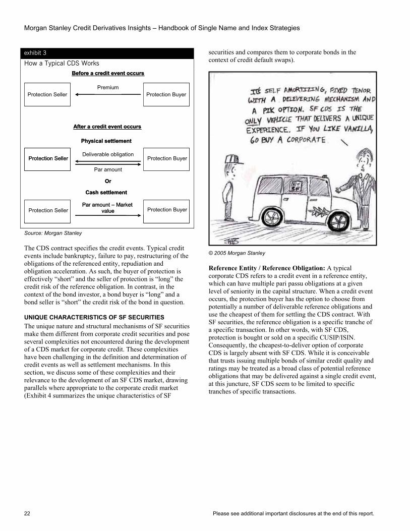
Morgan Stanley Credit Derivatives Insights – Handbook of Single Name and Index Strategies
22 Please see additional important disclosures at the end of this report.
exhibit 3
How a Typical CDS Works
Protection Seller
Before a credit event occurs
Deliverable obligationProtection Seller Protection Buyer
Premium
After a credit event occurs
Physical settlement
Par amount
Or
Protection Seller Protection Buyer
Cash settlement
Par amount – Market value
Protection BuyerProtection Seller
Before a credit event occurs
Deliverable obligationProtection Seller Protection Buyer
Premium
After a credit event occurs
Physical settlement
Par amount
Or
Protection Seller Protection Buyer
Cash settlement
Par amount – Market value
Protection Buyer
Source: Morgan Stanley
The CDS contract specifies the credit events. Typical credit events include bankruptcy, failure to pay, restructuring of the obligations of the referenced entity, repudiation and obligation acceleration. As such, the buyer of protection is effectively “short” and the seller of protection is “long” the credit risk of the reference obligation. In contrast, in the context of the bond investor, a bond buyer is “long” and a bond seller is “short” the credit risk of the bond in question.
UNIQUE CHARACTERISTICS OF SF SECURITIES The unique nature and structural mechanisms of SF securities make them different from corporate credit securities and pose several complexities not encountered during the development of a CDS market for corporate credit. These complexities have been challenging in the definition and determination of credit events as well as settlement mechanisms. In this section, we discuss some of these complexities and their relevance to the development of an SF CDS market, drawing parallels where appropriate to the corporate credit market (Exhibit 4 summarizes the unique characteristics of SF
securities and compares them to corporate bonds in the context of credit default swaps).
© 2005 Morgan Stanley
Reference Entity / Reference Obligation: A typical corporate CDS refers to a credit event in a reference entity, which can have multiple pari passu obligations at a given level of seniority in the capital structure. When a credit event occurs, the protection buyer has the option to choose from potentially a number of deliverable reference obligations and use the cheapest of them for settling the CDS contract. With SF securities, the reference obligation is a specific tranche of a specific transaction. In other words, with SF CDS, protection is bought or sold on a specific CUSIP/ISIN. Consequently, the cheapest-to-deliver option of corporate CDS is largely absent with SF CDS. While it is conceivable that trusts issuing multiple bonds of similar credit quality and ratings may be treated as a broad class of potential reference obligations that may be delivered against a single credit event, at this juncture, SF CDS seem to be limited to specific tranches of specific transactions.
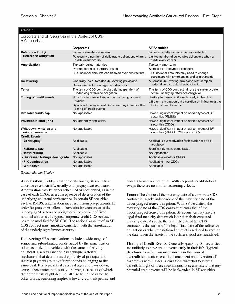
Section A, Chapter 2 Understanding Synthetic Structured Finance – First Steps
Please see additional important disclosures at the end of this report. 23
exhibit 4
Corporate and SF Securities in the Context of CDS: A Comparison
Corporates SF Securities Reference Entity/
Reference Obligation Issuer is usually a company. Potentially a number of deliverable obligations when a
credit event occurs
Issuer is usually a special purpose vehicle. Limited number of deliverable obligations when a
credit event occurs Amortization Typically bullet maturities
Prepayment risk is largely absent CDS notional amounts can be fixed over contract life
Typically amortizing Significant prepayment exposure CDS notional amounts may need to change
consistent with amortization and prepayments De-levering Generally, no automated de-levering provisions.
De-levering is by management discretion Automatic de-levering provisions with complex
waterfall and structural subordination Tenor The term of CDS contract largely independent of
underlying reference obligation The term of CDS contract mirrors the maturity date
of the underlying reference obligation Timing of credit events Structure has limited impact on the timing of credit
eventsSignificant management discretion may influence the
timing of credit events
Unlikely to have credit events early in their life Little or no management discretion on influencing the
timing of credit events
Available funds cap Not applicable Have a significant impact on certain types of SF securities (RMBS)
Payment-in-kind (PIK) Not generally applicable Have a significant impact on certain types of SF securities (CDOs)
Writedown, write up and reimbursements
Not applicable Have a significant impact on certain types of SF securities (RMBS, CMBS and CDOs)
Credit Events - Bankruptcy Applicable Applicable but motivation for inclusion may be
regulatory - Failure to pay Applicable Significantly more complicated - Restructuring Applicable Not applicable - Distressed Ratings downgrade Not applicable Applicable – not for CMBS - PIK continuation Not applicable Applicable – for CDOs - Writedown Not applicable Applicable
Source: Morgan Stanley
Amortization: Unlike most corporate bonds, SF securities amortize over their life, usually with prepayment exposure. Amortization may be either scheduled or accelerated, as in the case of cash CDOs, as a consequence of deterioration of the underlying collateral performance. In certain SF securities such as RMBS, amortization may result from pre-payments. In order for protection sellers to have similar economics as the underlying SF reference obligations, the concept of fixed notional amounts of a typical corporate credit CDS contract has to be modified for SF CDS. The notional amount of an SF CDS contract must amortize consistent with the amortization of the underlying reference security.
De-levering: SF securitizations include a wide range of senior and subordinated bonds issued by the same trust or other securitization vehicle with the same underlying collateral. Each transaction has a unique waterfall mechanism that determines the priority of principal and interest payments to the different bonds belonging to the same deal. It is typical that as a deal ages and pays down, some subordinated bonds may de-lever, as a result of which their credit risk might decline, all else being the same. In other words, seasoning implies a lower credit risk profile and
hence a lower risk premium. With corporate credit default swaps there are no similar seasoning effects.
Tenor: The choice of the maturity date of a corporate CDS contract is largely independent of the maturity date of the underlying reference obligation. With SF securities, the maturity date of the CDS contract mirrors that of the underlying reference obligation. SF securities may have a legal final maturity date much later than their expected maturity date. As such, the maturity date of SF CDS contracts is the earlier of the legal final date of the reference obligation or when the notional amount is reduced to zero or the date when the assets in the collateral pool are liquidated.
Timing of Credit Events: Generally speaking, SF securities are unlikely to have credit events early in their life. Typical structures have built-in mechanisms in the form of overcollateralization, credit enhancement and diversion of cash flows within a deal’s cash flow waterfall to avert a default. In light of these mechanisms, it seems likely that any potential credit events will be back-ended in SF securities.
Morgan Stanley Credit Derivatives Insights – Handbook of Single Name and Index Strategies
24 Please see additional important disclosures at the end of this report.
A notable difference between corporate credit and SF securities is the fact that in SF securities the built-in mechanisms mentioned above kick in automatically, with little discretion to the trustee or manager of the transaction. With a corporation, the management can potentially exercise a degree of control to affect the timing of a credit event, which is largely absent in SF securities.
Available Funds Cap (AFC): In general, US home equity loan ABS are floating rate instruments with coupon resets linked to an index such as LIBOR. Their underlying home loans are generally fixed rate or hybrid adjustable-rate mortgages (fixed for the initial 2-5 years and floating thereafter), with periodic and lifetime caps. Because of this embedded interest rate risk, US home equity loan securitizations include a feature that limits interest payments on a tranche if the level of the applicable floating index rate plus margin rises above a certain pre-specified rate, called the available funds cap rate,4 which is effectively the weighted average coupon of the underlying home equity loans. Therefore, when bond coupon rates rise above the AFC rate, there will be a shortfall in the interest payments received by the holders of the reference obligation, exposing them to interest rate risk unless there is enough excess interest in the deal to cover it.
Whether or not such interest rate risk is to be transferred to the sellers of protection in a CDS contract on an SF security has been a point of disagreement among market participants in the still-evolving SF CDS market. If the CDS contract is to mimic the economics of the underlying reference obligation, AFC risk has to be passed on as a part of the CDS contract. However, it introduces an element of interest rate risk to the CDS contract. We return to this topic in a later section to discuss the alternative ways this issue is being addressed.
Payment-in-Kind (PIK): Some SF securities, notably junior tranches of CDOs, permit the deferral of a scheduled coupon by increasing the outstanding principal balance of the transaction. Such a deferral may be temporary, caused by a cash flow mismatch in a deal and cured in a short period of time or permanent. If deferral continues over an extended period, it may trigger a credit event. Frequently, the risk of a PIK security is passed on to the seller of protection in a CDS contract by adjusting the fixed payment amounts paid by the protection buyer (CDS premium) by the PIK interest amount. When the reference obligation reverts to being current on its coupon and pays the accrued interest including the PIK-ed interest amount, such payments are passed back to the seller of protection.
Writedowns and Allocation of Losses: The principal balance of SF securities may be written down prior to their maturity date if losses experienced on the underlying 4This feature, while commonly prevalent in US home equity loan securitization, can also be seen in European CMBS and some US RMBS.
collateral pool exceed available credit enhancement for the tranche or if some portion of the principal is used to cover an interest shortfall. A principal writedown may not always occur before the maturity date, but some transactions (for example, European SF securitizations) provide for a principal deficiency ledger (PDL) to be used in place of an actual writedown. This accounting ledger is debited when losses in a given tranche exceed available credit enhancement and is credited if and when such losses are reversed. This creates an effective writedown in place of an actual writedown.
In practice, such writedowns may be either temporary – if the writedown is due to a short-term liquidity crunch and the principal written down is paid back to investors – or permanent when the deterioration in the collateral pool is severe enough and there is no possibility of an eventual recovery. For rated SF securities, rating agencies prescribe guidelines to determine when a writedown should be deemed permanent.5
Clean-Up Calls: Many securitization transactions have a provision by which the originator of a transaction can buy back the outstanding securitized instruments when the outstanding collateral balance has been substantially amortized, leaving a small amount of collateral to be serviced, which is often uneconomical. Usually, clean-up calls are exercised when the outstanding collateral balance falls below 10% of the original. In order to induce such clean-up calls to be exercised, there is usually a significant step-up in the coupon rate in the event the call is not exercised. In the event of such a step-up, the SF CDS protection buyer has the option to tear-up the contract. If the protection buyer chooses not to exercise that option, SF CDS premium also steps up. This is yet another characteristic unique to SF CDS, without a similar counterpart in the standard corporate CDS contract.
There are other more mundane differences as well. Payment dates on SF CDS are not standardized along the lines of corporate CDS (i.e., 20th of March, June, September and December). SF CDS payments dates are set to be five business days after the reference obligation’s coupon payment dates.
Given the many unique characteristics of SF securities discussed above, it follows that the mechanics of SF CDS, in terms of credit events and settlement mechanisms will be different from those of their corporate counterparts.
SF CDS: CREDIT EVENTS The meaning and the interpretation of a credit event in SF CDS may be significantly different from the same in 5For instance, in order to classify a writedown as permanent, Fitch requires the appointment of a qualified third-party to project the future performance of an SF security, the prevailing rating for the security to be less than an applicable rating threshold, and the effective writedown to have been in existence for a material period of time. (See “Synthetic Structured Finance CDOs,” Fitch Ratings, February 17, 2004.)
Section A, Chapter 2 Understanding Synthetic Structured Finance – First Steps
Please see additional important disclosures at the end of this report. 25
corporate CDS. As mentioned earlier, the three most common credit events for corporate CDS are bankruptcy, failure-to-pay and different variations of restructuring. Restructuring as a credit event is not meaningful for SF CDS. However, ratings downgrade, writedown and PIK continuation are frequently included as credit events within SF CDS. We discuss each of these credit events below.
Bankruptcy: Recall that unlike corporate issuers, bankruptcy-remote special purpose vehicles issue SF securities. Given that the sole raison d’être for the special purpose vehicle is to issue and service the SF securities based on a specifically delineated collateral pool of assets and there are no other businesses associated with the issuer, it is difficult to imagine bankruptcy as a credit event for SF securities. Notwithstanding this point, a Standard & Poor’s survey of synthetic CDO of ABS documentation found that 44% of the sample transactions included bankruptcy as a credit event.6 Satisfying regulatory capital requirements appears to be the motivation for the inclusion of bankruptcy as a credit event.
Failure-to-Pay: In a corporate CDS, failure-to-pay is easy to characterize and is triggered when the reference entity fails to make a payment when due, in excess of a specified threshold after the allowable grace period. With SF CDS, a failure-to-pay credit event is more complicated in two ways.
First, regarding principal payments, with the exception of the legal final maturity date, SF securities do not have a pre-defined schedule of dates when payments must be made. Instead, principal payments are “passed through” from the underlying collateral as and when available. Therefore, even when a default appears imminent, a failure-to-pay of principal may be determinable with certainty only at the legal final maturity date or upon an early termination of the referenced SF securities.
Second, the threshold should be specified such that superfluous, non-credit-related events do not trigger a credit event.7 At the same time, it is also necessary to ensure that the threshold is consistent with the tranche size, which could be significantly small in some cases.
In view of these complexities, the likelihood of a failure-to-pay event being triggered appears remote. However, from the perspective of a protection buyer, the inclusion of ratings downgrade and writedown as credit events might help mitigate the risks of failure to pay principal and/or interest since it is likely that they precede the triggering of a failure-to-pay event.
6See “Synthetic CDOs of ABS Documents Evolving Towards a Standard but Nuances Remain,” Standard and Poor’s, April 26, 2005. 7A report by Standard and Poor’s suggests the threshold to be $10,000. (See “Structural Issues in CDOs with Synthetic ABS Exposure,” Standard and Poor’s, March 7, 2005.)
Distressed Ratings Downgrade: A ratings downgrade does not constitute a credit event with corporate CDS. For SF CDS, ratings downgrade as a credit event may be extremely valuable from the perspective of protection buyers in that it might capture credit risks not captured in other credit events and be better reflective of the economic risks of a holder of the SF security in cash form. Ratings related triggers may be stand-alone or in some instances used in conjunction with other credit events. Standard & Poor’s has determined that in ABS transactions, a rating of CCC- is commensurate with default. The level at which a ratings downgrade credit event is triggered is often set above CCC- (or the equivalent Moody’s rating).
Under the present documentation a downgrade of the reference obligation by any rating agency to Caa2 or below (Moody’s ratings scale) or CCC or below (S&P/Fitch ratings scale) triggers a credit event. If the reference obligation had an original rating of Baa3 (or BBB-) or higher, it will have three months to recover to Caa1 (or CCC+) before a ratings downgrade credit event is triggered. For the purpose of a downgrade credit event, withdrawn ratings (not reinstated within five business days) are considered downgrades below the specified rating level.
Writedown: As long as the reference obligation does not provide for a reinstatement or reimbursement of written-down principal or does not pay interest on the written-down principal until reinstatement or reimbursement of principal, the occurrence of a writedown constitutes a credit event.
The determination of a writedown often rests with the calculation agent. Once a reference obligation is written down, the written-down amount is also the loss amount that the protection sellers owe protection buyers without any additional valuation mechanism to be put into place. Writedown as a credit event is not relevant in the context of pay-as-you-go, described in the next section.
SF CDS: SETTLEMENT MECHANISMS Upon the occurrence of a credit event, the protection buyer may deliver a credit event notice to the protection seller and settle all or any portion of the notional amount. There are essentially three settlement mechanisms for settling credit events with SF CDS – physical settlement, cash settlement and pay-as-you-go. There appears to be a “continental divide” of preferences in terms of settlement mechanisms: European transactions seem more inclined towards physical settlement with a cash settlement option, while US transactions lean towards pay-as-you-go settlements with a physical delivery option.
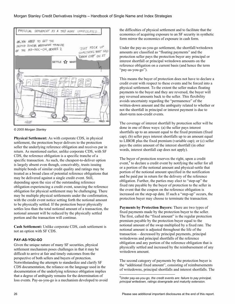
Morgan Stanley Credit Derivatives Insights – Handbook of Single Name and Index Strategies
26 Please see additional important disclosures at the end of this report.
© 2005 Morgan Stanley
Physical Settlement: As with corporate CDS, in physical settlement, the protection buyer delivers to the protection seller the underlying reference obligation and receives par in return. As mentioned earlier, unlike corporate CDS, with SF CDS, the reference obligation is a specific tranche of a specific transaction. As such, the cheapest-to-deliver option is largely absent even though, conceivably, trusts issuing multiple bonds of similar credit quality and ratings may be treated as a broad class of potential reference obligations that may be delivered against a single credit event. Still, depending upon the size of the outstanding reference obligation experiencing a credit event, sourcing the reference obligation for physical settlement may be challenging. There may be multiple physical settlements under the confirmation, with the credit event notice setting forth the notional amount to be physically settled. If the protection buyer physically settles less than the total notional amount of a transaction, the notional amount will be reduced by the physically settled portion and the transaction will continue.
Cash Settlement: Unlike corporate CDS, cash settlement is not an option with SF CDS.
PAY-AS-YOU-GO Given the unique nature of many SF securities, physical settlement mechanism poses challenges in that it may be difficult to arrive at fair and timely outcomes from the perspective of both sellers and buyers of protection. Notwithstanding the attempts to standardize and clarify SF CDS documentation, the reliance on the language used in the documentation of the underlying reference obligation implies that a degree of ambiguity remains for the determination of loss events. Pay-as-you-go is a mechanism developed to avoid
the difficulties of physical settlement and to facilitate that the economics of acquiring exposure to an SF security in synthetic form mirror the economics of exposure in cash form.
Under the pay-as-you-go settlement, the shortfall/writedown amounts are classified as “floating payments” and the protection seller pays the protection buyer any principal or interest shortfall or principal writedown amounts on the reference obligation on a current basis (and hence the term “pay-as-you-go”).
This means the buyer of protection does not have to declare a credit event with respect to these events and be forced into a physical settlement. To the extent the seller makes floating payments to the buyer and they are reversed, the buyer will pay reversed amounts back to the seller. This flexibility avoids uncertainty regarding the “permanence” of the written-down amount and the ambiguity related to whether or not the shortfall in principal or interest payment is due to short-term non-credit events.
The coverage of interest shortfall by protection seller will be done in one of three ways: (a) the seller pays interest shortfalls up to an amount equal to the fixed premium (fixed cap); (b) seller pays interest shortfalls up to an amount equal to LIBOR plus the fixed premium (variable cap); or (c) seller pays the entire amount of the interest shortfall (in other words, interest shortfall cap does not apply).
The buyer of protection reserves the right, upon a credit event,8 to declare a credit event by notifying the seller for all or a portion of the notional amount and physical-settle that portion of the notional amount specified in the notification and be paid par in return for the delivery of the reference obligation. Further, the parties may elect to “step-up” the fixed rate payable by the buyer of protection to the seller in the event that the coupon on the reference obligation is increased on the step-up date. If such a “step-up” occurs, the protection buyer may choose to terminate the transaction.
Payments by Protection Buyers: There are two types of fixed payments made by the protection buyer to the seller. The first, called the “fixed amount” is the regular protection premium payable by the protection buyer equal to the notional amount of the swap multiplied by a fixed rate. The notional amount is adjusted throughout the life of the transaction – decreased by principal payments, principal writedowns and principal shortfalls of the reference obligation and any portion of the reference obligation that is physically settled and increased by the reimbursement of any writedown amount.
The second category of payments by the protection buyer is the “additional fixed amount”, consisting of reimbursements of writedowns, principal shortfalls and interest shortfalls. The 8Under pay-as-you-go, the credit events are: failure to pay principal, principal writedown, ratings downgrade and maturity extension.
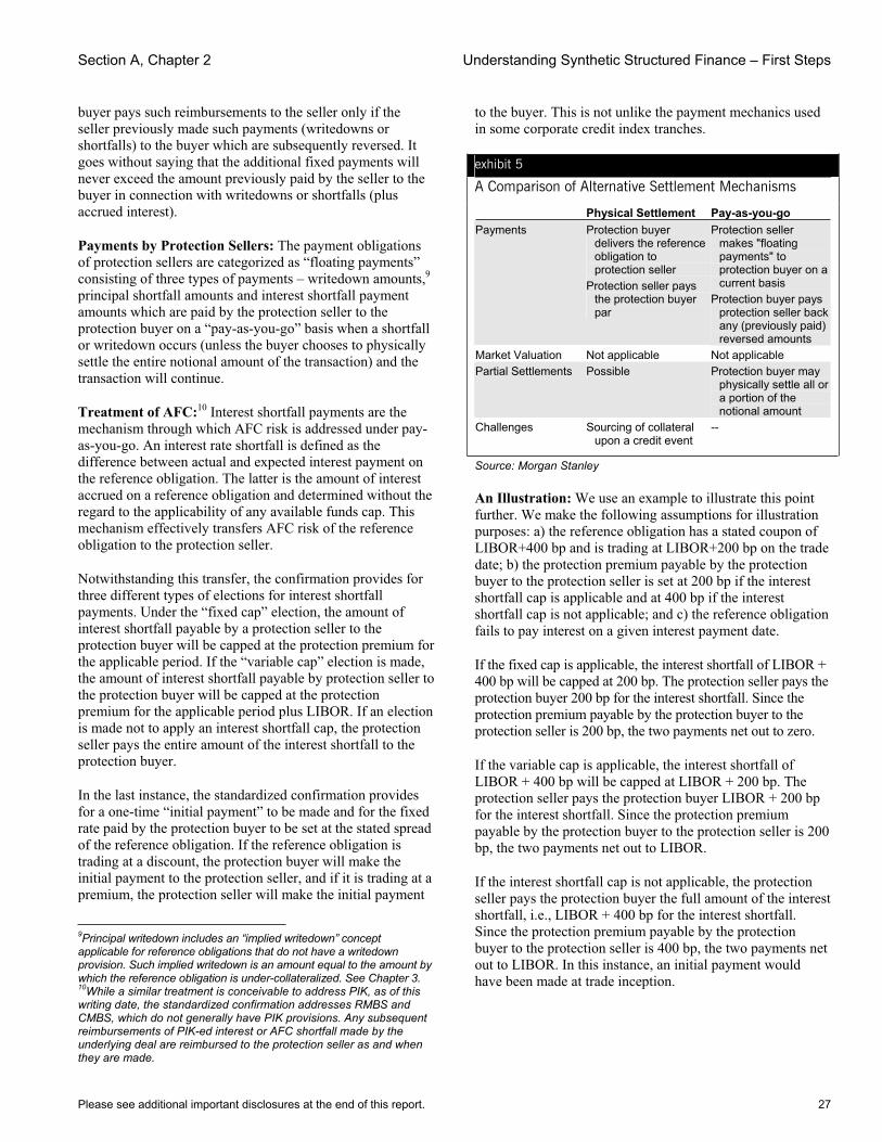
Section A, Chapter 2 Understanding Synthetic Structured Finance – First Steps
Please see additional important disclosures at the end of this report. 27
buyer pays such reimbursements to the seller only if the seller previously made such payments (writedowns or shortfalls) to the buyer which are subsequently reversed. It goes without saying that the additional fixed payments will never exceed the amount previously paid by the seller to the buyer in connection with writedowns or shortfalls (plus accrued interest).
Payments by Protection Sellers: The payment obligations of protection sellers are categorized as “floating payments” consisting of three types of payments – writedown amounts,9principal shortfall amounts and interest shortfall payment amounts which are paid by the protection seller to the protection buyer on a “pay-as-you-go” basis when a shortfall or writedown occurs (unless the buyer chooses to physically settle the entire notional amount of the transaction) and the transaction will continue.
Treatment of AFC:10 Interest shortfall payments are the mechanism through which AFC risk is addressed under pay-as-you-go. An interest rate shortfall is defined as the difference between actual and expected interest payment on the reference obligation. The latter is the amount of interest accrued on a reference obligation and determined without the regard to the applicability of any available funds cap. This mechanism effectively transfers AFC risk of the reference obligation to the protection seller.
Notwithstanding this transfer, the confirmation provides for three different types of elections for interest shortfall payments. Under the “fixed cap” election, the amount of interest shortfall payable by a protection seller to the protection buyer will be capped at the protection premium for the applicable period. If the “variable cap” election is made, the amount of interest shortfall payable by protection seller to the protection buyer will be capped at the protection premium for the applicable period plus LIBOR. If an election is made not to apply an interest shortfall cap, the protection seller pays the entire amount of the interest shortfall to the protection buyer.
In the last instance, the standardized confirmation provides for a one-time “initial payment” to be made and for the fixed rate paid by the protection buyer to be set at the stated spread of the reference obligation. If the reference obligation is trading at a discount, the protection buyer will make the initial payment to the protection seller, and if it is trading at a premium, the protection seller will make the initial payment
9Principal writedown includes an “implied writedown” concept applicable for reference obligations that do not have a writedown provision. Such implied writedown is an amount equal to the amount by which the reference obligation is under-collateralized. See Chapter 3. 10While a similar treatment is conceivable to address PIK, as of this writing date, the standardized confirmation addresses RMBS and CMBS, which do not generally have PIK provisions. Any subsequent reimbursements of PIK-ed interest or AFC shortfall made by the underlying deal are reimbursed to the protection seller as and when they are made.
to the buyer. This is not unlike the payment mechanics used in some corporate credit index tranches.
exhibit 5
A Comparison of Alternative Settlement Mechanisms
Physical Settlement Pay-as-you-go Payments Protection buyer
delivers the reference obligation to protection seller
Protection seller pays the protection buyer par
Protection seller makes "floating payments" to protection buyer on a current basis
Protection buyer pays protection seller back any (previously paid) reversed amounts
Market Valuation Not applicable Not applicable Partial Settlements Possible Protection buyer may
physically settle all or a portion of the notional amount
Challenges Sourcing of collateral upon a credit event
--
Source: Morgan Stanley
An Illustration: We use an example to illustrate this point further. We make the following assumptions for illustration purposes: a) the reference obligation has a stated coupon of LIBOR+400 bp and is trading at LIBOR+200 bp on the trade date; b) the protection premium payable by the protection buyer to the protection seller is set at 200 bp if the interest shortfall cap is applicable and at 400 bp if the interest shortfall cap is not applicable; and c) the reference obligation fails to pay interest on a given interest payment date.
If the fixed cap is applicable, the interest shortfall of LIBOR + 400 bp will be capped at 200 bp. The protection seller pays the protection buyer 200 bp for the interest shortfall. Since the protection premium payable by the protection buyer to the protection seller is 200 bp, the two payments net out to zero.
If the variable cap is applicable, the interest shortfall of LIBOR + 400 bp will be capped at LIBOR + 200 bp. The protection seller pays the protection buyer LIBOR + 200 bp for the interest shortfall. Since the protection premium payable by the protection buyer to the protection seller is 200 bp, the two payments net out to LIBOR.
If the interest shortfall cap is not applicable, the protection seller pays the protection buyer the full amount of the interest shortfall, i.e., LIBOR + 400 bp for the interest shortfall. Since the protection premium payable by the protection buyer to the protection seller is 400 bp, the two payments net out to LIBOR. In this instance, an initial payment would have been made at trade inception.

Morgan Stanley Credit Derivatives Insights – Handbook of Single Name and Index Strategies
28 Please see additional important disclosures at the end of this report.
exhibit 6
Transfer of AFC Risk: An Illustration i) Fixed cap applicable
200 bp(capped interest shortfall)
200 bp (protection premium)
ii) Variable cap applicableLIBOR + 200 bp
(capped interest shortfall)
200 bp (protection premium)
iii) Interest shortfall cap not applicable LIBOR + 400 bp
(entire interest shortfall)
400 bp (protection premium)
Protection Buyer Protection Seller
Net Payment = Zero
Protection Buyer Protection Seller
Net Payment = LIBOR
Protection Buyer Protection Seller
Net Payment = LIBOR
i) Fixed cap applicable200 bp
(capped interest shortfall)
200 bp (protection premium)
ii) Variable cap applicableLIBOR + 200 bp
(capped interest shortfall)
200 bp (protection premium)
iii) Interest shortfall cap not applicable LIBOR + 400 bp
(entire interest shortfall)
400 bp (protection premium)
Protection Buyer Protection Seller
Net Payment = Zero
Protection Buyer Protection Seller
Net Payment = LIBOR
Protection Buyer Protection Seller
Net Payment = LIBOR
Note: Under (iii) above, an initial payment would have been made at trade inception.
Source: Morgan Stanley
THE TOTAL RETURN SWAP (TRS) ALTERNATIVE An alternative to CDS structures for SF securities is to enter into a total return swap. A TRS can be funded or unfunded and involves two counterparties (A and B, for this illustration). In the funded form, counterparty A pays counterparty B the notional amount of the transaction on the effective date of the transaction and receives payments that exactly mirror the underlying reference obligation throughout the remaining life of the transaction as well as the price appreciation or depreciation of the underlying reference obligation.
In its unfunded form, there is no upfront payment. Instead, counterparty A makes periodic floating rate payments (LIBOR plus or minus a spread) and receives cash flows that exactly mirror the underlying reference obligation throughout the remaining life of the transaction as well as the price appreciation or depreciation of the underlying reference obligation. The maturity date of the TRS is generally set to match the legal final maturity date of the underlying reference obligation. The difference between a CDS structure and a TRS structure is that the latter includes a price return component and the former does not.
SF CDS: PRICING AND BASIS RELATIONSHIPS Notwithstanding the many unique features of SF securities and the complexities of SF CDS, the basic principles of risk-
neutral pricing remain similar to corporate CDS pricing11 and the CDS premium reflects the expected cost of providing protection in a risk-neutral sense. The fair SF CDS premium equals the present value of expected losses or payments made under the provisions of the SF CDS under the risk-neutral measure. Still, given the unique characteristics of SF securities and the complexities of alternative credit events and the many variations in settlement mechanisms, implementing a theoretical pricing model for SF CDS in a risk neutral framework is bound to be more intricate and is beyond the scope of this chapter.
However, analogous to Z spread in corporate bonds, with SF securities we can use the discount margins (DM) to define a basis relationship between cash and synthetic instruments. Recall that unlike corporate bonds, SF securities are typically floating rate instruments. DM is a pricing analytic associated with floating rate instruments and represents the margin relative to the benchmark index rate of the SF security that makes its current price equal to the discounted present value of its cash flows. In the context of SF CDS, the difference between the CDS premium of a reference obligation and its DM represents the basis between synthetic and cash instruments. If the economics of risk exposure to a specific reference obligation in cash form or synthetic form through CDS are identical, the basis would be zero. However, just as is the case with corporate CDS, there are several reasons for the basis to be different from zero.
While the concept of a “credit curve” with CDS trading to different maturities is common in corporate CDS, a comparable concept does not exist for SF CDS at this stage, mainly because SF CDS contracts do not have bullet maturities. Still, from what we know about the timing of losses in ABS, particularly in HEL ABS, we can reasonably posit that due to the back-loaded nature of losses, embedded credit curves in SF CDS are theoretically fairly steep.
Finally, there is a potential for survivor bias in portfolios of ABS securities such as indices and bespoke pools. Well-performing collateral pools prepay sooner – and consequently portfolios decline in their average credit quality over time because of prepayments.
SF CDS: APPLICATIONS Just as the introduction of CDS opened new avenues for the implementation of sophisticated hedging and investment strategies, there is a tremendous potential for their application within the broad arena of structured finance securities. SF CDS enable investors to be both long and short exposure and express directional views on specific securities or, more broadly, SF sectors, an opportunity that was hitherto difficult to implement. It would be possible to acquire exposure to assets that were difficult to source in the cash market as well as hedge existing exposures for better risk 11See Chapter 1 for a detailed exposition of risk neutral pricing as applied to CDS pricing.

Section A, Chapter 2 Understanding Synthetic Structured Finance – First Steps
Please see additional important disclosures at the end of this report. 29
management and achieve efficient allocation of economic and regulatory capital.
Further, SF CDS enable investors to obtain leveraged exposures and use synthetic CDO technology to customize and manage the amount of such leverage. In fact, CDOs are natural sellers of protection within the SF CDS market, given the long ramp-up time increasingly noticed in SF CDOs due to the paucity of the collateral in the cash market. SF CDS also contribute towards an expansion of the collateral universe for a CDO manager to choose from, resulting in better diversified portfolios and better managed risks than would be possible if totally constrained to cash instruments.
To a large extent, this is already happening. Synthetic buckets in SF CDOs have increased significantly over the last year. Hybrid SF CDOs, which provide the flexibility for managers to obtain collateral in cash or synthetic form, are an emerging trend in SF CDOs. Managed synthetic SF CDOs, as well as credit default swaps on managed and static pools in SF portfolios, have also been on the rise. According to data complied by Creditflux, a UK-based provider of news and analysis for credit derivatives and the structured credit market, $94 billion of ABS-referenced portfolio credit default swaps were done during 2005. Standardization of documentation should, in our opinion, provide additional impetus to this phenomenon.
Arrangers of CDOs, and more generally, warehousers of securitization products, would be natural buyers of protection. Even if SF CDS were to achieve only a fraction of the market acceptance of their corporate counterparts, it would still mean that a brave new world of opportunities has been opened for SF market participants.
FROM ABS CDS TO ABX INDICES Following the success of credit derivatives indices in the corporate credit market, the development of benchmark indices based on credit default swaps on structured finance securities was the next step in a logical progression of events in the evolution of synthetic structured finance. The first such group of benchmark indices, called ABX.HE, were launched in January 2006, focusing on the home equity ABS sector.
The objective of these indices is to create liquid, transparent and standardized CDS benchmarks that will allow a broad range of investors to obtain exposure to the different ABS sectors, express directional views on them, efficiently hedge risk exposures and employ trading strategies. Each of these benchmark indices will have a portfolio of credit default swaps referencing a standardized basket of reference
obligations. Such portfolios will be constructed using an objective, rules-based approach to promote transparency with a third-party administrator12 providing daily prices and valuation analytics. Credit default swaps included in each of these indices will use standardized documentation to promote operational efficiency.
ABX.HE OVERVIEW ABX.HE represents a series of standardized indices for CDS on a basket of 20 recent home equity securitization transactions, with five ratings-based sub-indices for AAA, AA, A, BBB and BBB- rating categories. Each sub-index consists of a portfolio of 20 credit default swaps, each referencing a specific cash bond from each of the 20 home equity securitization deals. While reference obligations are equally weighted in the portfolio at the launch of the series, the subsequent portfolio composition may change depending upon on the performance of the underlying pools (pre-payments, defaults and amortizations, etc.). There are no substitutions allowed in the underlying portfolio over time.
DIFFERENCES BETWEEN ABX.HE AND SF CDS The mechanics of the ABX.HE are similar to single-name SF CDS with a few important exceptions. First, while the single-name SF CDS documentation provides for alternative mechanisms for dealing with shortfalls (fixed cap, variable cap and no cap alternatives as described earlier), CDS referencing the ABX.HE will only have a fixed cap convention. Second, the pay-as-you-go mechanism applies but without the option for physical settlement if there is a credit event. Third, the treatment of the clean-up call is different. SF CDS contracts provide for optional termination of the CDS if the underlying transaction is not called, and if the CDS remains in effect, the premium usually steps up. With the ABX.HE, there is no optional termination provision when a clean-up call is not exercised and there is no step-up in premium.
ABX.HE MECHANICS Consistent with the pay-as-you-go approach, the obligation of the protection seller is to cover interest shortfall amounts up to the premium payments and any principal shortfall and write-down amounts of the reference obligations in the portfolio. Without the optional physical settlement provision, the maturity of the ABX.HE is effectively the maturity of the longest CDS within the underlying portfolio. The payments from the buyer and seller of protection are summarized in Exhibit 7 below.
12Markit is the administration, calculation and marketing agent for the ABX series of indices.

Morgan Stanley Credit Derivatives Insights – Handbook of Single Name and Index Strategies
30 Please see additional important disclosures at the end of this report.
exhibit 7
Payments by Protection Buyers and Sellers on ABX.HE
Protection Buyer (Fixed Rate Payer)
Protection Seller (Floating Rate Payer)
Pays a monthly premium (quoted as basis points per annum) to the protection seller on notional amount• The notional amount will decline
over time based on the reference obligation amortization and any principal writedown
Receives a monthly premium (quoted as basis points per annum) from the protection buyer on notional amount • The notional amount will decline
over time based on the reference obligation amortization and principal writedown
Receives payments from the protection seller in the event of the following • Interest shortfall (capped at the
fixed rate) • Principal shortfall • Writedown
Pays the protection buyer in the event of the following • Interest shortfall (capped at the
fixed rate) • Principal shortfall • Writedown
Pays to the protection seller in the event of the following • Interest shortfall reimbursement
amount• Principal shortfall reimbursement
amount• Writedown reimbursement amount
Receives from the protection buyer in the event of the following • Interest shortfall reimbursement
amount• Principal shortfall reimbursement
amount• Writedown reimbursement amount
Source: Morgan Stanley
To further illustrate the changes to the notional amount and payments in the event of a writedown, consider the following scenario. Say the fixed rate paid by the protection buyer on a notional of $100 million is 70 bps; at index inception the factor on the reference obligation was 1.0 and is now 0.75; and a writedown in the amount of 1% of the current principal balance occurs in year 3. The writedown amount is calculated as the product of (current factor * weighting of the reference obligation in the index * the writedown %) and the notional amount. In our example, this equals $37,500 = (0.75 * 0.05 * 0.01) * $100 mm. The index notional amount will be reduced by 0.0375% and subsequent fixed payments (70 bp) by the protection buyer will be on the remaining index notional amount.
ABX.HE TRADES ON PRICE, NOT SPREAD Since there are no standard prepayment conventions, and since different investors make different prepayment assumptions resulting in different durations for the underlying reference obligations, trading the indices on spread terms can be complicated. Consequently, the ABX.HE indices trade on price terms. Each index has a predetermined premium that is fixed (as a percentage of notional) over the life of the index. Index prices will be quoted in a typical bond convention, as a percentage of par and any premium or discount is exchanged upfront. To illustrate this, assume that the index is at 100 and the index fixed rate is the market spread. If on a subsequent trade date the index is at 98, it means that the implied spreads have widened. For a trade initiated that day, the protection buyer pays the protection seller 2% * notional * current factor. On the other hand, if on that trade date, the index is at 102, it means that the implied spreads have tightened and the
protection seller pays the protection buyer 2% * notional * current factor.
ABX.HE: PORTFOLIO CONSTRUCTION13
The portfolio of reference obligations for each ABX.HE series will be constructed such that the index is representative of the sub-prime home equity market. The third-party administrator will submit to each participating dealer two deals from the largest 25 sub-prime home equity bond issuers based on the following criterion:
(a) Issued within the previous six months.
(b) Minimum issue offering size of $500 million.
(c) At least 90% of the deal’s assets must be first lien mortgages.
(d) Weighted average FICO score of the borrowers in the pool < 660
(e) Referenced tranches must be floating rate payers indexed to one-month LIBOR
(f) At issuance, each deal must have tranches with ratings of each of the sub-indices with an average life greater than four years, except for the AAA tranche, which must have an average life greater than five years
(g) All tranches rated by both S&P and Moody’s – if split rated, the lower rating will apply
On the following day, each participating dealer will send to the third-party administrator a ranking of their deal preference for each issuer from the list provided. Based on this, the administrator will create a master list of 20 deals such that the list meets the concentration criteria that it contains no more than four deals with loans from the same originator and no more than six deals from the same master servicer.
One day before the index creation date, each participating dealer will submit the fixed rate for each index, and the average of all such submissions (after discarding the top and bottom quartiles) will be the fixed rate for each index. The composition of each index series will be published four days prior to the creation of each new index series. Each index will contain the same list of reference obligations until all reference obligations are fully paid off or have matured.
At the outset, the intention was for a new series of ABX to be issued every six months to reference a new set of home equity securitization transactions. As we go to print, we are unsure whether future index rolls will continue at the current frequency, given the recent issues in the ABS market.
13This section is largely drawn from the ABX Rules, January 17, 2006, available at http://www.markit.com/abx.jsp

Section A, Chapter 2 Understanding Synthetic Structured Finance – First Steps
Please see additional important disclosures at the end of this report. 31
NEXT STEPS On an analytical front, a significant benefit of the growth and liquidity in corporate CDS markets has been the ability to obtain market-implied forward-looking default probabilities based on CDS premiums. Hitherto, there was no clean way of isolating the credit risk component from the interest rate component using the market prices of credit risky fixed income securities. It has now become commonplace to discuss the credit risk of corporates in terms of CDS premiums. While some of the unique features of SF securities make such a clean isolation harder, improved
liquidity in SF CDS should be a step in the right direction for improved transparency and analytics.
In conclusion, we revert to the point we made at the outset of this chapter. Current efforts toward standardization of documentation for SF CDS are likely to result in innovative ways for transferring credit risk, implementing hedging strategies and expanding investment opportunities for a wide range of market participants in the structured finance market. Synthetics are now more than just a niche within the structured finance world.
Morgan Stanley Credit Derivatives Insights – Handbook of Single Name and Index Strategies
32 Please see additional important disclosures at the end of this report.
Chapter 3
CDS on CDOs: Back to the Future
Primary Analyst: Vishwanath Tirupattur Primary Analyst: Sivan Mahadevan
First came cash CDOs, way back in the late 1980s, as a first step in structured credit. Then came credit default swaps (CDS) on corporates, which rose from humble beginnings in the mid-to-late 1990s to become the de facto standard instrument for the corporate credit market today. Along the way, CDS went through a major growing up process driven by cyclical downturns in credit during 1997-2002, which made it possible for testing the then-fledgling CDS market. This led to standardization of contract terms, which further impelled liquidity and resulted in the widespread acceptance of CDS across a broad range of market participants today. It is fair to say that the much-discussed bespoke structured credit bid today is a direct consequence of the successful emergence of CDS as the instrument of choice in the corporate credit arena. Development of corporate CDS spawned the growth of CDS referencing other asset classes such as asset-backed securities (ABS) and leveraged loans. In each case, CDS documentation evolved to take into consideration the idiosyncrasies of the respective markets.
The release of an ISDA standard template for ABS CDS during June 2005 was a landmark development. A year later, the release of an ISDA standard template for CDS referencing cash CDO tranches completed the circle that started in the late 1980s. The “street standard” documentation that came out in June 2006 has provided an impetus for secondary trading of CDO tranches.
In this chapter, we discuss the main features of the ISDA template for CDS on CDOs, contrasting them with the ABS CDS mechanics, and we identify CDS applications for taking both long and short positions in the cash CDO market.
CDS ON ABS VERSUS CDS ON CDOS: WHAT IS DIFFERENT?Cash CDOs are a special case of asset-backed securities and share many unique characteristics with ABS, such as waterfall mechanisms, structural delevering, amortization, write-downs, and PIK, among others. As such, the broad chassis of the CDS contract developed for ABS CDS, most notably Pay-As-You-Go mechanics,1 is very much applicable to CDS on cash CDO tranches, as well. A few important features of the standardized template for CDS on CDOs are worth noting.
First, unlike the ABS CDS contract, CDS on CDO contemplates “implied write-down” as an electable credit event or a pay-as-you-go event. Implied write-down for
1See Chapter 2.
CDOs is effectively when the value of the over-collateralization ratio for the tranche falls below one.
Second, the interest shortfall clause – fixed cap, variable cap and no-cap – applies for CDO tranches as well. As with ABS CDS, the applicable cap is an election. However, the context of interest shortfall may be different for cash CDOs, compared to ABS. Unlike ABS, where interest shortfall is more likely to result from available funds cap provisions, thereby introducing an element of interest rate risk in a CDS contract, interest shortfalls with CDO tranches are more likely to be a result of deteriorating credit performance of the underlying collateral rather than the level of interest rates. As such, interest rate risk as a trigger for the shortfall is of secondary significance.
Third, the failure to pay interest credit event has an additional condition to settlement meant to take into consideration the PIK-ability feature common in mezzanine CDO tranches. If the reference obligation is PIK-able, it is a condition for settlement that at least 360 calendar days have elapsed since the occurrence of the failure to pay interest credit event without the relevant interest shortfall having been reimbursed in full. In other words, for a PIK-able reference obligation, for failure to pay interest to become a credit event, PIK-ed interest should not have been reimbursed in full for more than 360 days.
Finally, the step-up coupon and WAC cap concepts are not pertinent to CDO securities and hence not a feature of the CDS on CDO contract.
Apart from these distinguishing features, the rest of the ISDA standardized template is largely similar to the ABS CDS contract. The contract specifies a particular reference obligation, as opposed to a reference entity. The reference obligation is identified by its CUSIP or ISIN, legal final maturity date, original principal amount, initial factor, coupon, the reference entity and insurer, if any. The notional amount amortizes consistent with the amortization of the reference obligation. The protection buyer is the sole credit event notifying party. The standard credit events are as follows: failure to pay principal, failure to pay interest, distressed ratings downgrade and write-down. The applicability, or lack thereof, of implied write-down is an election at the inception of the CDS contract.
In case the buyer of protection declares a credit event for part of or the entire notional amount, this would result in a full or partial physical settlement. However, given the challenges of sourcing securities for physically settling CDS contracts, Pay-As-You-Go has emerged as the mechanism of choice for CDOs, as well.

Section A, Chapter 3 CDS on CDOs: Back to the Future
Please see additional important disclosures at the end of this report. 33
In our judgment, the choice of ‘variable cap’ and ‘no implied writedown’ makes the economics of the CDS contract most similar to that of the cash instrument.
APPLICATIONS We think that synthetics on cash CDOs open up a brave new world of opportunities for cash CDO investors. Most significantly, they offer a mechanism to go long, as well as short, cash CDO tranches, which have traditionally been a long-only market. CDS enable investors to express directional views on specific CDO tranches, CDO managers and more broadly CDO sectors, an opportunity that was hitherto difficult to implement. Buying protection on specified tranches of ABS CDOs as a means of expressing negative views on the US housing market and subprime HEL securitization has been a particularly successful strategy for several investors. Similarly, expressing a leveraged short view on the loan market was implemented successfully by some investors through being long protection on specified CLO tranches.
Another application of the CDS on CDO has been to acquire exposure to CDO securities that were difficult to source in the cash market, as well as to explore long-short strategies
within the cash CDO space. Hedging existing exposures for better risk management and achieving efficient allocation of economic and regulatory capital is yet another application of CDS on CDOs.
Further, CDS on CDOs pave the way for investors to obtain leveraged exposures and use synthetic CDO technology to customize and manage the amount of such leverage. In addition to the obvious CDO-squared applications, CDS on CDOs also contribute towards an expansion of the collateral universe for a CDO manager – of cash or synthetic or hybrid CDOs.
CONCLUSIONThe standardization of documentation of CDS on cash CDOs is a significant development. In our judgment, this has the potential to infuse liquidity and increase secondary trading of cash CDOs. In this chapter, we have barely scratched the surface of the many opportunities to go long and short in this space and to implement interesting strategies for acquiring CDO risk and managing CDO risk exposure.
We acknowledge the contributions of Simmi Sareen to this chapter.

Morgan Stanley Credit Derivatives Insights – Handbook of Single Name and Index Strategies
34 Please see additional important disclosures at the end of this report.
Chapter 4
Leveraged Loan CDS: A First Step Up
Primary Analyst: Vishwanath Tirupattur Primary Analyst: Sivan Mahadevan Primary Analyst: Peter Polanskyj
INTRODUCTIONMuch of the innovation in the corporate credit markets over the past decade has been either in derivatives (CDS), structures (CBOs and CLOs) or combinations of both (synthetic structured credit). One major development in the single-name cash markets has been in leveraged loans, which, in their two main forms (bank and institutional loans), have experienced tremendous growth over the past few years. As demand has increased for exposure to secured high yield credit, there has been an important shift from bank loans to those targeted to institutional investors. As such, the investor base in leveraged loans has grown both directly (specialized funds and traditional high yield investors) and indirectly (CLOs, which have replaced CBOs as the preferred method of gaining structured exposure to high yield credit).
Loans used to be seen as arcane, clubby, documentation-intensive bilateral instruments with limited liquidity and secondary trading opportunities. This perception is changing. Syndicated loans have emerged as the dominant way for issuers to tap banks and other institutional capital providers for loans. The adoption of market-flex language – which allowed arrangers to change the pricing and other terms based on investor demand, is often seen1 as the impetus for transforming the loan markets into the full-fledged capital markets we know them as today. Credit default swaps (CDS) referencing loans are the latest innovation in this market, which we expect to have a transformational impact on loan markets and, more broadly, corporate and structured credit markets. While leveraged loan CDS does have much in common with corporate CDS by virtue of the 2003 ISDA Credit Derivatives Definitions, there are important distinctions as well, both structurally and geographically.
In this chapter, we will discuss the unique characteristics of the loan market and highlight differences between bonds and loans to motivate a discussion of CDS on secured loans contrasted with the established CDS market for unsecured debt.2 Furthermore, we will describe the mechanics and features of the leveraged loan CDS contract (as it looks today) emphasizing the differences between the US and European
1See Standard and Poor’s “A Guide to the Loan Market,” September 2004 for a historical exposition. In later sections of this publication, we will draw upon the Standard and Poor’s publication to discuss certain features of the loan markets and their terminology. 2We will refer to the standard CDS on unsecured instruments, such as corporate bonds, throughout this publication as corporate CDS.
markets.3 We will also discuss the factors that determine basis relationships between cash and synthetic instruments, as well as between corporate CDS and leveraged loan CDS. Finally, we discuss the applications of leveraged loan CDS from different perspectives. Note that we use the terms “leveraged loan,” “secured loan” and even simply “loan” interchangeably in this chapter.
From a derivatives perspective, we want to make it clear upfront that plenty of evolution and maturing needs to occur for any standardized leveraged loan CDS contract. We feel the market is very much in the early stages, which readers will hopefully gather as they go through this publication, and we fully expect future credit events and the like to provide teething pains and to help create more mature contracts as the market moves forward.
exhibit 1
Global New-Issue Leveraged Loan Volume
$ Billion
0
100
200
300
400
500
600
700
1998 1999 2000 2001 2002 2003 2004 2005 2006
USA Non-USA
Source: S&P LCD
WHY LEVERAGED LOAN CDS? The market for secured loans has been booming for the last few years on both sides of the Atlantic (Exhibit 1). Record-breaking new issuance volumes amidst ever-tightening spreads, driven by the explosive growth in CLOs, as well as leveraged finance transactions, have been the hallmark of secured loans business. At the same time, significant changes are afoot that could have profound impacts on this market, with reverberations that could be felt in the broader corporate credit market. These include changes in the regulatory capital regime due to Basel II creating new demand for hedging bank loan exposures, changes to rating agency approaches to
3See our European colleagues’ report ”Leveraged Loan CDS: The Final Piece of the Jigsaw,” November 4, 2005, for details on European loans and CDS.

Section A, Chapter 4 Leveraged Loan CDS: A First Step Up
Please see additional important disclosures at the end of this report. 35
better distinguish the performance of secured loans as opposed to unsecured bonds, and growing institutionalization of the market, particularly in Europe.
The consistent and stable performance of the loan market (to date) has generated a large expansion of investor interest and consequent cash inflows into the loan market. The returns from loan investing as reflected in the S&P LSTA Loan Index over the last several years have been impressive in absolute terms (Exhibit 2). Further, measured on a risk-adjusted basis using Sharpe ratios, loans compare favorably relative to other competing asset classes (see Exhibit 3, based on S&P LCD data).
exhibit 2
Total Return of S&P LSTA Index (1997-2006)
0%
2%
4%
6%
8%
10%
12%
1997 1998 1999 2000 2001 2002 2003 2004 2005 2006
Source: S&P LCD
exhibit 3
Sharpe Ratio: S&P LSTA Index versus Other Asset Classes (1997-2006)
0.0
0.2
0.4
0.6
0.8
1.0
S&P LSTAIndex
ML High YieldBond Index
10 YTreasuries
S&P 500 Index ML HighGrade Bond
Index
Source: S&P LCD
As the credit cycle appears to be on the cusp of turning, credit investors have demonstrated a shift in sentiment to
move higher up in the capital structure by shifting from unsecured bonds to secured loans. This, coupled with the insatiable demand from CLOs, has made access to loans in the cash form a major constraint for investors trying to get long exposures to secured loans as an asset class. However, we caution that recovery value is a zero sum game, so to the degree that secured loans take the place of unsecured bonds in the capital structure, the historically high recoveries of loans are not sustainable.
At the same time, another section of investors is concerned with what is seen as declining credit quality, lack of diversity across CLO portfolios and exposure to LBOs embedded in the loan market; these investors seek instruments to short the loan market or efficiently hedge their exposures. In addition, commercial and investment banks require instruments that enable them to maintain relationships with issuers while simultaneously managing the capital risks of corporate lending.
Well constructed, standardized synthetic instruments can efficiently address these many demands from the long and short sides of this evolving market. Just as the development of CDS in corporate, emerging market and, more recently, asset-backed securities has radically transformed the underlying markets, development of a loan CDS contract has the potential to be similarly transformative for the loan sector. Current industry-wide efforts to develop a standardized contract for loan CDS are a natural outgrowth of these evolving dynamics in the marketplace for secured loans, paving the way for innovative methods of transferring risk, implementing hedging strategies and expanding opportunities for a wide range of market participants.
UNIQUE CHARACTERISTICS OF THE LEVERAGED LOAN MARKET Floating Rate Instruments: Leveraged loans are typically floating rate payers with an interest amount equal to a floating rate index that is periodically reset (usually quarterly) plus a fixed spread (margin). Bonds may have either fixed or floating coupons.
Ratings: Most bonds are rated by at least one rating agency. While it is a lot more common for US loans to be rated as well, European loans frequently do not carry public ratings.
Loan Structure: The majority of loans may be structured as one of two categories – revolving credit facilities and term loans. A revolver is a commitment to make loans to a borrower up to the maturity date of the facility, and a borrower may borrow and repay a revolving credit facility multiple times until the maturity of the facility at the discretion of the borrower. Revolvers are generally unfunded and mainly used by investment grade borrowers. A term loan is funded at closing and any repayment results in a permanent reduction in outstanding amount, i.e., no re-borrowing. Because of the largely unfunded nature of the revolvers, they are not traded frequently.

Morgan Stanley Credit Derivatives Insights – Handbook of Single Name and Index Strategies
36 Please see additional important disclosures at the end of this report.
There are two principal categories of term loans – amortizing term loans and institutional term loans. An amortizing term loan (“TLA”) is a fully funded term loan with a specified amortization schedule (usually weighted towards the later years); it is generally syndicated to banks, along with revolvers, as a part of larger syndications. Institutional term loans (“TLB”, “TLC”, “TLD,” etc.) are the type of loans that are of most interest to institutional lenders who generally do not maintain a relationship with the borrowers; these constitute the bulk of the traded loans and, as such, are the category of loans that will be of most interest in the context of loan CDS. Institutional term loans are secured, rank pari passu with other facilities, and usually have interest margins higher than revolvers or TLAs, repaid mostly in a bullet form (scheduled amortization, if any, is minimal and significantly back-ended). In addition, institutional term loans are longer dated (with maturities of five to seven years) but may be prepaid at any time at par (unless specifically structured with call protections) and used by leveraged borrowers (non-investment-grade borrowers with Debt/EBITDA greater than 2.0x). Multiple tranches with varying maturities can co-exist within a facility (TLB, TLC, TLD, and so on, are labeled as such for each maturity). The vast majority of the loan market is comprised of institutional loans.
While these structures (especially term loans) have some similarity to corporate bonds by way of differing maturities, their security, amortization and prepayability features are unique to loans.
Seniority and Security: Loans almost always rank senior to other parts of the debt capital structure. For non-investment-grade borrowers, they are also secured by all tangible and intangible assets of the borrower in the form of pledges of collateral. In some cases, loans are secured by specific assets. The secured and senior nature of leveraged loans is an extremely important feature that determines the recovery prospects for a loan if there is a default. Historically, the average recovery rates for secured loans have been significantly higher than unsecured debt (Exhibit 4).
exhibit 4
Average Recovery Rates for Corporate Debt Obligors (1982-2005)
1982-2005Loans Senior Secured 70.0% Senior Unsecured 57.6%Bonds Senior Secured 51.9% Senior Unsecured 36.0% Senior Subordinated 32.4% Subordinated 31.8% Junior Subordinated 23.9%
Source: “Default and Recovery Rates of Corporate Bond Issuers, 1920-2005,” Moody’s Investors Service, January 2006.
In this context, it is useful to discuss another growing type of syndicated leveraged loans – second-lien loans. As implied by their name, claims on second-liens rank behind those of the first-lien loans and, as such, trade at significantly wider premiums to first-lien loans. The recovery potential for second-lien loans is usually lower. The term “designated priority” is used to designate the lien status (whether the loan is first lien or second lien).
Covenants: A defining feature of leveraged loans, as opposed to bonds, is the significant and onerous set of restrictions on borrowers imposed through covenant protections. While there is a wide gamut of such restrictions specified in loan agreements, in general, the riskier the borrower, the larger the covenant package. Covenants can be affirmative (actions borrowers must take to be compliant with a loan), negative (limitations on the types and amounts of new debt, liens, asset sales, acquisitions, parent/subsidiary guarantees) and financial (enforcing minimum financial performance measures). Financial covenants can include limitations on coverage (minimum cash flow/earnings relative to interest and debt service), leverage (maximum level of debt relative to cash flow or earnings), current-ratio (minimum ratio of current assets to current liabilities), tangible net-worth (minimum levels of tangible assets excluding assets such as good will and intellectual assets) and maximum capital expenditure (limiting the purchase of property, plans and equipment).
The extent of covenant protection is critical in determining the riskiness of the borrower. While bonds, especially non-investment grade bonds, also have some form of such covenants, they are not typically as onerous as with loans. It is worth emphasizing that there is a wide variation in covenant packages across loan agreements. Furthermore, second lien loans typically have less restrictive covenant packages and maintenance covenants are set wide of the first lien loans.
Secondary Trading Conventions: Once a loan transaction is closed upon primary issuance, it can be traded in the secondary market. Such sales can be structured in one of two forms – assignments or participations. The differences between the two forms are mainly in terms of rights, as well as the degree of documentation and consents that need to be sought and obtained. Assignments usually require the consent of the borrower and the agent on a not-to-be-unreasonably-withheld basis; the assignee becomes the direct signatory to the loan and receives interest and principal payments from the administrative agent of the loan agreement. In the event of a borrower default, assignees will have complete rights and access to private information as lenders of record.
Participations do not have the consent requirements of assignments, and a buyer obtaining a loan through participation enters into a separate agreement with an
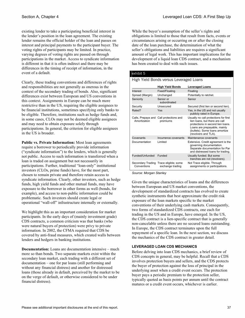
Section A, Chapter 4 Leveraged Loan CDS: A First Step Up
Please see additional important disclosures at the end of this report. 37
existing lender to take a participating beneficial interest in the lender’s position in the loan agreement. The existing lender remains the official holder of the loan and passes on interest and principal payments to the participant buyer. The voting rights of participants may be limited. In practice, varying degrees of voting rights are passed on through participations in the market. Access to syndicate information is different in that it is often indirect and there may be differences in the timing of receipt of information, in the event of a default.
Clearly, these trading conventions and differences of rights and responsibilities are not generally as onerous in the context of the secondary trading of bonds. Also, significant differences exist between European and US conventions in this context. Assignments in Europe can be much more restrictive than in the US, requiring the eligible assignees to be financial institutions, sometimes specifying only banks to be eligible. Therefore, institutions such as hedge funds and, in some cases, CLOs may not be deemed eligible assignees and may need to obtain exposure solely through participations. In general, the criterion for eligible assignees in the US is broader.
Public vs. Private Information: Most loan agreements require a borrower to periodically provide information (“syndicate information”) to the lenders, which is generally not public. Access to such information is transferred when a loan is traded on assignment but not necessarily in participations. Further, traditional “loan-only” institutional investors (CLOs, prime funds) have, for the most part, chosen to remain private and therefore retain access to syndicate information. Clearly, other investors, such as hedge funds, high yield funds and other mutual funds, may have exposure to the borrower in other forms as well (bonds, for example), and access to non-public information could be problematic. Such investors should create legal or operational “wall-off” infrastructure internally or externally.
We highlight this as an important consideration for market participants. In the early days of (mainly investment grade) CDS contracts, a common criticism was that banks (who were natural buyers of protection) were privy to private information. In 2002, the CFMA required that CDS be covered by anti-fraud measures, which created walls between lenders and hedgers in banking institutions.
Documentation: Loans are documentation intensive – much more so than bonds. Two separate markets exist within the secondary loan market, each trading with a different set of documentation – one for par loans (still performing and without any financial distress) and another for distressed loans (those already in default, perceived by the market to be on the verge of default, or otherwise considered to be under financial distress).
While the buyer’s assumption of the seller’s rights and obligations is limited to those that result from facts, events or circumstances arising or occurring on or after the closing date of the loan purchase, the determination of what the seller’s obligations and liabilities are requires a significant amount of legal work. This has important implications for the development of a liquid loan CDS contract, and a mechanism has been created to deal with such issues.
exhibit 5
High Yield Bonds versus Leveraged Loans
High Yield Bonds Leveraged Loans Interest Fixed/Floating FloatingSpread (Margin) Unchanged Potentially to ratchet. Seniority Senior or
subordinated Senior
Security Unsecured Secured (first lien or second lien).Rated? Yes Yes, in the US and not usually
publicly rated in Europe. Calls, Prepays and
Amortization Call protections and
premiumsUsually no call protections for first
lien loans, but there are call protections in second lien loans. Loans are prepayable, mainly (bullets). Some loans amortize (revolvers and TLA).
Covenants Incurrence covenants Maintenance covenants Documentation Limited Extensive. Credit agreement is the
governing documentation. Separate documentation for Par and distressed loans for trading.
Funded/Unfunded Funded Usually funded. But some tranches are not (revolvers).
Secondary Trading Conventions
Trace eligible; some exchange trading
Not Trace eligible. Through assignments or participations.
Source: Morgan Stanley
Given the unique characteristics of loans and the differences between European and US market conventions, the development of standardized contracts has evolved to create synthetic instruments that best approximate the credit risk exposure of the loan markets specific to the market conventions of their underlying cash markets. Consequently, two forms of standardized CDS contracts, one each for trading in the US and in Europe, have emerged. In the US, the CDS contract is a lien-specific contract that is generally non-cancelable unless there are no secured loans outstanding. In Europe, the CDS contract terminates upon the full repayment of a specific loan. In the next section, we discuss the mechanics of the CDS contract in greater detail.
LEVERAGED LOAN CDS MECHANICS Before delving into loan CDS mechanics, a brief review of CDS concepts in general, may be helpful. Recall that a CDS involves protection buyers and sellers, and the CDS protects the buyer of protection against the loss of principal in the underlying asset when a credit event occurs. The protection buyer pays a periodic premium to the protection seller, typically quoted as basis points per annum until the contract matures or a credit event occurs, whichever is earlier.
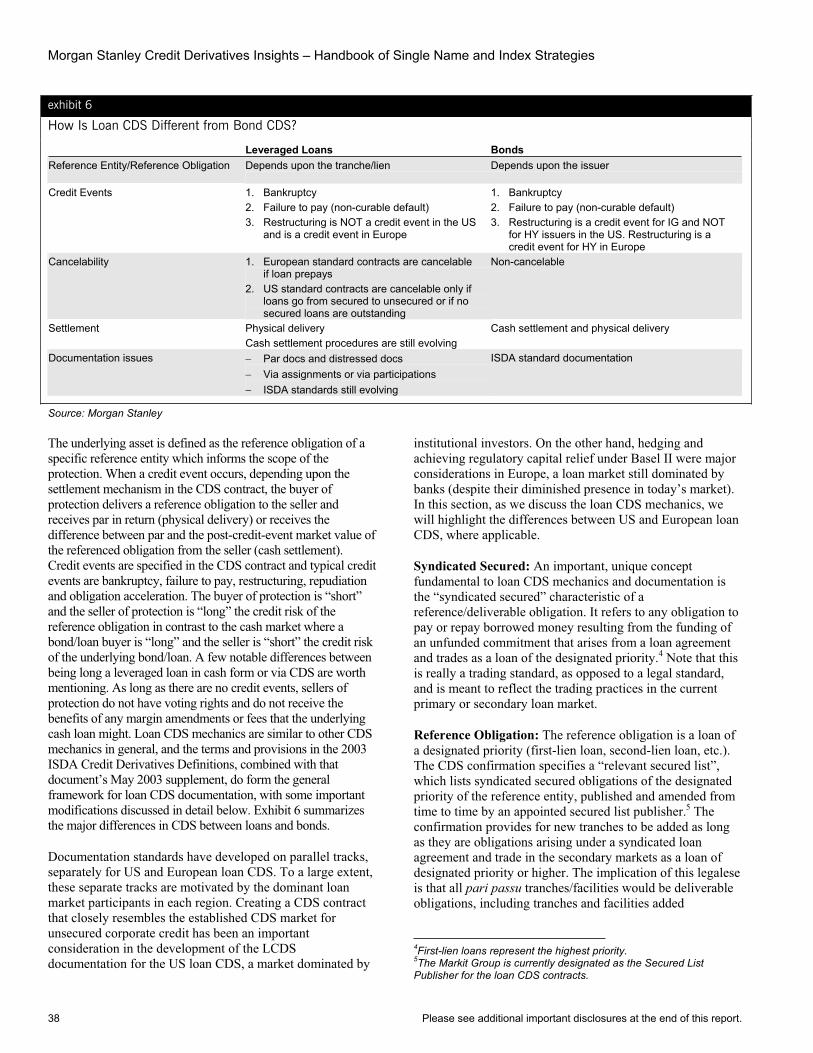
Morgan Stanley Credit Derivatives Insights – Handbook of Single Name and Index Strategies
38 Please see additional important disclosures at the end of this report.
exhibit 6
How Is Loan CDS Different from Bond CDS?
Leveraged Loans Bonds Reference Entity/Reference Obligation Depends upon the tranche/lien Depends upon the issuer
Credit Events 1. Bankruptcy 2. Failure to pay (non-curable default) 3. Restructuring is NOT a credit event in the US
and is a credit event in Europe
1. Bankruptcy 2. Failure to pay (non-curable default) 3. Restructuring is a credit event for IG and NOT
for HY issuers in the US. Restructuring is a credit event for HY in Europe
Cancelability 1. European standard contracts are cancelable if loan prepays
2. US standard contracts are cancelable only if loans go from secured to unsecured or if no secured loans are outstanding
Non-cancelable
Settlement Physical delivery Cash settlement procedures are still evolving
Cash settlement and physical delivery
Documentation issues − Par docs and distressed docs − Via assignments or via participations − ISDA standards still evolving
ISDA standard documentation
Source: Morgan Stanley
The underlying asset is defined as the reference obligation of a specific reference entity which informs the scope of the protection. When a credit event occurs, depending upon the settlement mechanism in the CDS contract, the buyer of protection delivers a reference obligation to the seller and receives par in return (physical delivery) or receives the difference between par and the post-credit-event market value of the referenced obligation from the seller (cash settlement). Credit events are specified in the CDS contract and typical credit events are bankruptcy, failure to pay, restructuring, repudiation and obligation acceleration. The buyer of protection is “short” and the seller of protection is “long” the credit risk of the reference obligation in contrast to the cash market where a bond/loan buyer is “long” and the seller is “short” the credit risk of the underlying bond/loan. A few notable differences between being long a leveraged loan in cash form or via CDS are worth mentioning. As long as there are no credit events, sellers of protection do not have voting rights and do not receive the benefits of any margin amendments or fees that the underlying cash loan might. Loan CDS mechanics are similar to other CDS mechanics in general, and the terms and provisions in the 2003 ISDA Credit Derivatives Definitions, combined with that document’s May 2003 supplement, do form the general framework for loan CDS documentation, with some important modifications discussed in detail below. Exhibit 6 summarizes the major differences in CDS between loans and bonds.
Documentation standards have developed on parallel tracks, separately for US and European loan CDS. To a large extent, these separate tracks are motivated by the dominant loan market participants in each region. Creating a CDS contract that closely resembles the established CDS market for unsecured corporate credit has been an important consideration in the development of the LCDS documentation for the US loan CDS, a market dominated by
institutional investors. On the other hand, hedging and achieving regulatory capital relief under Basel II were major considerations in Europe, a loan market still dominated by banks (despite their diminished presence in today’s market). In this section, as we discuss the loan CDS mechanics, we will highlight the differences between US and European loan CDS, where applicable.
Syndicated Secured: An important, unique concept fundamental to loan CDS mechanics and documentation is the “syndicated secured” characteristic of a reference/deliverable obligation. It refers to any obligation to pay or repay borrowed money resulting from the funding of an unfunded commitment that arises from a loan agreement and trades as a loan of the designated priority.4 Note that this is really a trading standard, as opposed to a legal standard, and is meant to reflect the trading practices in the current primary or secondary loan market.
Reference Obligation: The reference obligation is a loan of a designated priority (first-lien loan, second-lien loan, etc.). The CDS confirmation specifies a “relevant secured list”, which lists syndicated secured obligations of the designated priority of the reference entity, published and amended from time to time by an appointed secured list publisher.5 The confirmation provides for new tranches to be added as long as they are obligations arising under a syndicated loan agreement and trade in the secondary markets as a loan of designated priority or higher. The implication of this legalese is that all pari passu tranches/facilities would be deliverable obligations, including tranches and facilities added
4First-lien loans represent the highest priority. 5The Markit Group is currently designated as the Secured List Publisher for the loan CDS contracts.
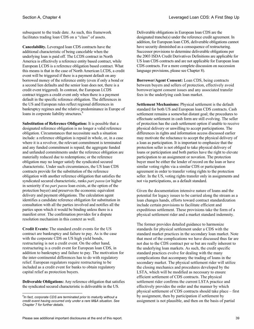
Section A, Chapter 4 Leveraged Loan CDS: A First Step Up
Please see additional important disclosures at the end of this report. 39
subsequent to the trade date. As such, this framework facilitates trading loan CDS on a “class” of assets.
Cancelability. Leveraged loan CDS contracts have the additional characteristic of being cancelable when the underlying loan is paid off. The LCDS contract in North America is effectively a reference entity based contract, while European LCDS is a reference obligation based contract. What this means is that in the case of North American LCDS, a credit event will be triggered if there is a payment default on any borrowed money of the reference entity (even if only a bond or a second lien defaults and the senior loan does not, there is a credit event triggered). In contrast, the European LCDS contract triggers a credit event only when there is a payment default in the specific reference obligation. The differences in the US and European rules reflect regional differences in bankruptcy regimes and the relative predominance in Europe of loans in corporate liability structures.6
Substitution of Reference Obligation: It is possible that a designated reference obligation is no longer a valid reference obligation. Circumstances that necessitate such a situation include: a reference obligation is repaid in whole, or, in a case where it is a revolver, the relevant commitment is terminated and any funded commitment is repaid; the aggregate funded and unfunded commitments under the reference obligation are materially reduced due to redemptions; or the reference obligation may no longer satisfy the syndicated secured characteristic. Under such circumstances, the US loan CDS contracts provide for the substitution of the reference obligation with another reference obligation that satisfies the syndicated secured characteristic, ranks pari passu (or higher in seniority if no pari passu loan exists, at the option of the protection buyer) and preserves the economic equivalent delivery and payment obligations. The calculation agent identifies a candidate reference obligation for substitution in consultation with all the parties involved and notifies all the parties upon which it would be binding unless there is a manifest error. The confirmation provides for a dispute resolution mechanism in this context as well.
Credit Events: The standard credit events for the US contract are bankruptcy and failure to pay. As is the case with the corporate CDS on US high yield bonds, restructuring is not a credit event. On the other hand, restructuring is a credit event for European loan CDS, in addition to bankruptcy and failure to pay. The motivation for the inter-continental differences has to do with regulatory relief. European regulators require restructuring to be included as a credit event for banks to obtain regulatory capital relief as protection buyers.
Deliverable Obligations: Any reference obligation that satisfies the syndicated secured characteristic is deliverable in the US. 6In fact, corporate CDS are terminated prior to maturity without a credit event having occurred only under a rare M&A situation. See Chapter 7 for further details.
Deliverable obligations in European loan CDS are the designated tranche(s) under the reference credit agreement. In addition, for European loan CDS, deliverable obligations cannot have security diminished as a consequence of restructuring. Successor provisions to determine deliverable obligations per the 2003 ISDA Credit Derivatives Definitions are applicable for US loan CDS contracts and are not applicable for European loan CDS contracts. For a more complete discussion on succession language provisions, please see Chapter 8).
Borrower/Agent Consent: Loan CDS, being contracts between buyers and sellers of protection, effectively avoid borrower/agent consent issues and any associated transfer fees in the underlying cash loan market.
Settlement Mechanisms: Physical settlement is the default standard for both US and European loan CDS contracts. Cash settlement remains a somewhat distant goal; the procedures to effectuate settlement in cash form are still evolving. The seller of protection has the cash settlement option if unable to receive physical delivery or unwilling to accept participations. The differences in rights and information access discussed earlier may motivate the reluctance to accept the physical delivery of a loan as participation. It is important to emphasize that the protection seller is not obliged to take physical delivery of loans or participation and both parties have the right to elevate participation to an assignment or novation. The protection buyer must be either the lender of record on the loan or have similar voting rights via a similar CDS or participation agreement in order to transfer voting rights to the protection seller. In the US, voting rights transfer only in assignments and not via participations, as a default standard.
Given the documentation intensive nature of loans and the potential for legacy issues to be carried along the stream as a loan changes hands, efforts toward contract standardization include certain provisions to facilitate efficient and expeditious settlement. These provisions take the form of a physical settlement rider and a market standard indemnity.
The former provides detailed guidance to harmonize standards for physical settlement under a CDS with the standard market practices in the secondary loan market. Note that most of the complications we have discussed thus far are not due to the CDS contract per se but are really inherent to the underlying loan markets. As such, the credit specific standard practices evolve for dealing with the many complications that accompany the trading of loans in the secondary market. The physical settlement rider will utilize the closing mechanics and procedures developed by the LSTA, which will be modified as necessary to ensure efficient settlement of CDS contracts. The physical settlement rider confirms the current LSTA practice and effectively provides the order and the manner by which physical settlement of CDS contracts should take place – first by assignment, then by participation if settlement by assignment is not plausible, and then on the basis of partial
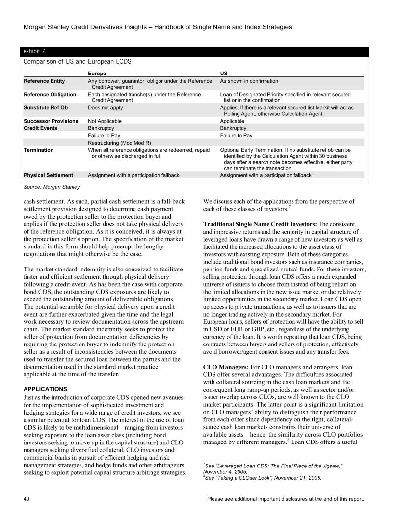
Morgan Stanley Credit Derivatives Insights – Handbook of Single Name and Index Strategies
40 Please see additional important disclosures at the end of this report.
exhibit 7
Comparison of US and European LCDS
Europe US Reference Entity Any borrower, guarantor, obligor under the Reference
Credit Agreement As shown in confirmation
Reference Obligation Each designated tranche(s) under the Reference Credit Agreement
Loan of Designated Priority specified in relevant secured list or in the confirmation
Substitute Ref Ob Does not apply Applies. If there is a relevant secured list Markit will act as Polling Agent, otherwise Calculation Agent.
Successor Provisions Not Applicable Applicable Credit Events Bankruptcy Bankruptcy
Failure to Pay Failure to Pay Restructuring (Mod Mod R)
Termination When all reference obligations are redeemed, repaid or otherwise discharged in full
Optional Early Termination: If no substitute ref ob can be identified by the Calculation Agent within 30 business days after a search note becomes effective, either party can terminate the transaction
Physical Settlement Assignment with a participation fallback Assignment with a participation fallback
Source: Morgan Stanley
cash settlement. As such, partial cash settlement is a fall-back settlement provision designed to determine cash payment owed by the protection seller to the protection buyer and applies if the protection seller does not take physical delivery of the reference obligation. As it is conceived, it is always at the protection seller’s option. The specification of the market standard in this form should help preempt the lengthy negotiations that might otherwise be the case.
The market standard indemnity is also conceived to facilitate faster and efficient settlement through physical delivery following a credit event. As has been the case with corporate bond CDS, the outstanding CDS exposures are likely to exceed the outstanding amount of deliverable obligations. The potential scramble for physical delivery upon a credit event are further exacerbated given the time and the legal work necessary to review documentation across the upstream chain. The market standard indemnity seeks to protect the seller of protection from documentation deficiencies by requiring the protection buyer to indemnify the protection seller as a result of inconsistencies between the documents used to transfer the secured loan between the parties and the documentation used in the standard market practice applicable at the time of the transfer.
APPLICATIONS Just as the introduction of corporate CDS opened new avenues for the implementation of sophisticated investment and hedging strategies for a wide range of credit investors, we see a similar potential for loan CDS. The interest in the use of loan CDS is likely to be multidimensional – ranging from investors seeking exposure to the loan asset class (including bond investors seeking to move up in the capital structure) and CLO managers seeking diversified collateral, CLO investors and commercial banks in pursuit of efficient hedging and risk management strategies, and hedge funds and other arbitrageurs seeking to exploit potential capital structure arbitrage strategies.
We discuss each of the applications from the perspective of each of these classes of investors.7
Traditional Single Name Credit Investors: The consistent and impressive returns and the seniority in capital structure of leveraged loans have drawn a range of new investors as well as facilitated the increased allocations to the asset class of investors with existing exposure. Both of these categories include traditional bond investors such as insurance companies, pension funds and specialized mutual funds. For these investors, selling protection through loan CDS offers a much expanded universe of issuers to choose from instead of being reliant on the limited allocations in the new issue market or the relatively limited opportunities in the secondary market. Loan CDS open up access to private transactions, as well as to issuers that are no longer trading actively in the secondary market. For European loans, sellers of protection will have the ability to sell in USD or EUR or GBP, etc., regardless of the underlying currency of the loan. It is worth repeating that loan CDS, being contracts between buyers and sellers of protection, effectively avoid borrower/agent consent issues and any transfer fees.
CLO Managers: For CLO managers and arrangers, loan CDS offer several advantages. The difficulties associated with collateral sourcing in the cash loan markets and the consequent long ramp-up periods, as well as sector and/or issuer overlap across CLOs, are well known to the CLO market participants. The latter point is a significant limitation on CLO managers’ ability to distinguish their performance from each other since dependency on the tight, collateral-scarce cash loan markets constrains their universe of available assets – hence, the similarity across CLO portfolios managed by different managers.8 Loan CDS offers a useful
7See “Leveraged Loan CDS: The Final Piece of the Jigsaw,” November 4, 2005. 8See “Taking a CLOser Look”, November 21, 2005.
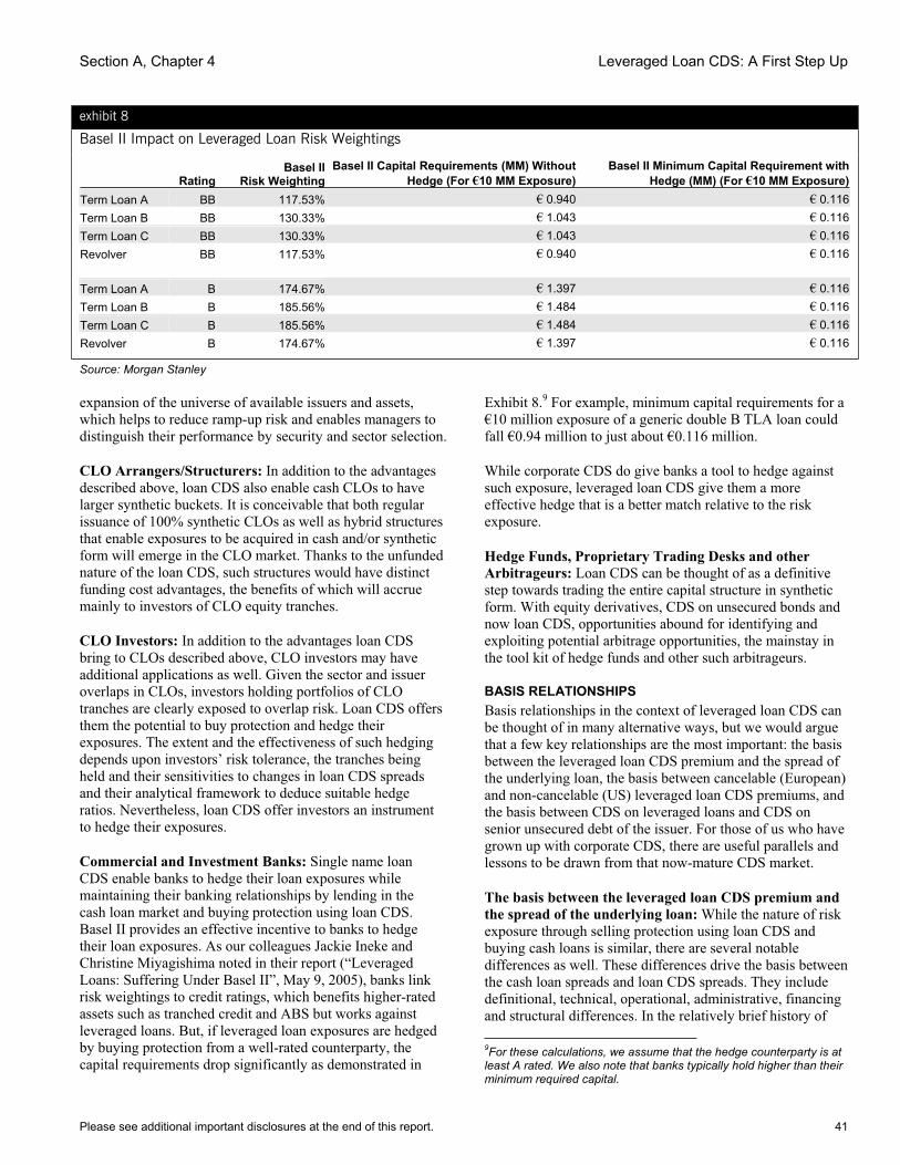
Section A, Chapter 4 Leveraged Loan CDS: A First Step Up
Please see additional important disclosures at the end of this report. 41
exhibit 8
Basel II Impact on Leveraged Loan Risk Weightings
Rating Basel II
Risk Weighting Basel II Capital Requirements (MM) Without
Hedge (For €10 MM Exposure)Basel II Minimum Capital Requirement with
Hedge (MM) (For €10 MM Exposure)Term Loan A BB 117.53% € 0.940 € 0.116Term Loan B BB 130.33% € 1.043 € 0.116Term Loan C BB 130.33% € 1.043 € 0.116Revolver BB 117.53% € 0.940 € 0.116 Term Loan A B 174.67% € 1.397 € 0.116Term Loan B B 185.56% € 1.484 € 0.116Term Loan C B 185.56% € 1.484 € 0.116Revolver B 174.67% € 1.397 € 0.116
Source: Morgan Stanley
expansion of the universe of available issuers and assets, which helps to reduce ramp-up risk and enables managers to distinguish their performance by security and sector selection.
CLO Arrangers/Structurers: In addition to the advantages described above, loan CDS also enable cash CLOs to have larger synthetic buckets. It is conceivable that both regular issuance of 100% synthetic CLOs as well as hybrid structures that enable exposures to be acquired in cash and/or synthetic form will emerge in the CLO market. Thanks to the unfunded nature of the loan CDS, such structures would have distinct funding cost advantages, the benefits of which will accrue mainly to investors of CLO equity tranches.
CLO Investors: In addition to the advantages loan CDS bring to CLOs described above, CLO investors may have additional applications as well. Given the sector and issuer overlaps in CLOs, investors holding portfolios of CLO tranches are clearly exposed to overlap risk. Loan CDS offers them the potential to buy protection and hedge their exposures. The extent and the effectiveness of such hedging depends upon investors’ risk tolerance, the tranches being held and their sensitivities to changes in loan CDS spreads and their analytical framework to deduce suitable hedge ratios. Nevertheless, loan CDS offer investors an instrument to hedge their exposures.
Commercial and Investment Banks: Single name loan CDS enable banks to hedge their loan exposures while maintaining their banking relationships by lending in the cash loan market and buying protection using loan CDS. Basel II provides an effective incentive to banks to hedge their loan exposures. As our colleagues Jackie Ineke and Christine Miyagishima noted in their report (“Leveraged Loans: Suffering Under Basel II”, May 9, 2005), banks link risk weightings to credit ratings, which benefits higher-rated assets such as tranched credit and ABS but works against leveraged loans. But, if leveraged loan exposures are hedged by buying protection from a well-rated counterparty, the capital requirements drop significantly as demonstrated in
Exhibit 8.9 For example, minimum capital requirements for a €10 million exposure of a generic double B TLA loan could fall €0.94 million to just about €0.116 million.
While corporate CDS do give banks a tool to hedge against such exposure, leveraged loan CDS give them a more effective hedge that is a better match relative to the risk exposure.
Hedge Funds, Proprietary Trading Desks and other Arbitrageurs: Loan CDS can be thought of as a definitive step towards trading the entire capital structure in synthetic form. With equity derivatives, CDS on unsecured bonds and now loan CDS, opportunities abound for identifying and exploiting potential arbitrage opportunities, the mainstay in the tool kit of hedge funds and other such arbitrageurs.
BASIS RELATIONSHIPS Basis relationships in the context of leveraged loan CDS can be thought of in many alternative ways, but we would argue that a few key relationships are the most important: the basis between the leveraged loan CDS premium and the spread of the underlying loan, the basis between cancelable (European) and non-cancelable (US) leveraged loan CDS premiums, and the basis between CDS on leveraged loans and CDS on senior unsecured debt of the issuer. For those of us who have grown up with corporate CDS, there are useful parallels and lessons to be drawn from that now-mature CDS market.
The basis between the leveraged loan CDS premium and the spread of the underlying loan: While the nature of risk exposure through selling protection using loan CDS and buying cash loans is similar, there are several notable differences as well. These differences drive the basis between the cash loan spreads and loan CDS spreads. They include definitional, technical, operational, administrative, financing and structural differences. In the relatively brief history of 9For these calculations, we assume that the hedge counterparty is at least A rated. We also note that banks typically hold higher than their minimum required capital.

Morgan Stanley Credit Derivatives Insights – Handbook of Single Name and Index Strategies
42 Please see additional important disclosures at the end of this report.
the LCDS market thus far, these differences have driven the basis between loan CDS spreads and cash loan spreads to be negative (cash loan spreads wider than LCDS premiums on the same obligors).
Cash loans are prepayable and often do prepay, in contrast to LCDS contracts that are designed to be non-cancellable. The prepayment option that the cash loan investors are “short” is valuable even in today’s environment of low implied volatility and is a significant determinant of the basis. In addition, loan holders benefit from being “long” covenants, amendment/fees and coupon flexes to which LCDS holders do not have access.
On the other hand, besides the obvious funding advantages, getting long risk exposure through LCDS contracts is far less operationally intensive compared to its cash counterpart.
However, these relationships could change when the credit cycle ultimately turns. When the spreads are wider, the call option investors are selling might be worth less. LCDS may widen more than cash loans in such an environment, as the LCDS contract would be the natural instrument to short loan risk. We provide a more comprehensive explanation of the LCDS basis in Chapter 38.
The basis between leveraged loan CDS and senior unsecured CDS of the issuer: The basis between CDS premiums on secured and unsecured parts of the capital structure of the same issuer will be a function of the basis between loans and unsecured debt, which itself is driven by a myriad of factors, the most important of which we list below:
1. The size of the borrowings at the various levels of seniority (loans, senior secured debt, senior unsecured debt, subordinated debt, etc.) relative to the total borrowings of the company.
2. The absolute likelihood of default for the issuer.
3. The relative quality of covenants of the loan and senior bond obligations.
4. The likelihood of any capital structure changes and relative pricing of the loan and bond portions of a new capital structure in any corporate restructuring.
5. Any differentials in maturity profiles between the loans and bonds of the issuer.
CONCLUSIONIf it feels like we covered a lot of ground in this chapter, we have our reasons. In our view, the community of investors with significant experience in both credit derivatives and leveraged loans is small, and therefore there are experience curves that most need to climb. Furthermore, credit derivatives tied to leveraged loans have unique issues that should result in some interesting tests of contract language over time. We are indeed excited about strategic opportunities in the secured high yield credit space involving both single-names and CLOs, as well as full capital structure plays. However, we do caution that we are in the early days of a market that will need time (and increased credit risk) to mature.

Section A, Chapter 4 Leveraged Loan CDS: A First Step Up
Please see additional important disclosures at the end of this report. 43
exhibit 9
Applications of Leveraged Loan CDS
Traditional Single Name Investors - Expanded universe of issuers - Ability to sell protection in different currencies in the European market - Avoid borrower/agent consent issues and transfer fees
CLO Managers - Shorter ramp-up periods - Expanded reference universe decreases sector/issuer overlap - Increased potential to distinguish performance by security and sector selection - Improved funding efficiency
CLO Arrangers/Structurers - Shorter ramp-up periods - Improved collateral sourcing thanks to expanded universe - Funding cost advantages will accrue to equity investors - Facilitate use of larger synthetic buckets (up to 100%)
CLO Investors - Hedge CLO exposure and minimize overlap risks - Funding cost advantages will accrue to equity investors - Shorter ramp-up periods - Expanded universe of issuers
Commercial and Investment Banks - Hedge loan exposure while maintaining banking relationships - Hedging reduces risk weightings and provides regulatory capital relief under Basel II regime - Proprietary trading opportunities
Hedge Funds, Prop Desks & Other Arbitrageurs - Capital structure arbitrage - Ability to short credit in the loan space - Risk management and minimization of overlap risks - Expanded universe of issuers - Avoid borrower/agent consent issues and transfer fees
Source: Morgan Stanley
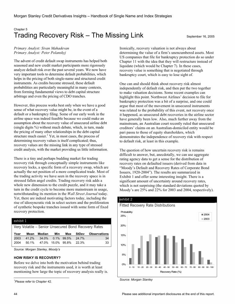
Morgan Stanley Credit Derivatives Insights – Handbook of Single Name and Index Strategies
44 Please see additional important disclosures at the end of this report.
Chapter 5
Trading Recovery Risk – The Missing Link September 16, 2005
Primary Analyst: Sivan Mahadevan Primary Analyst: Peter Polanskyj
The advent of credit default swap instruments has helped both seasoned and new credit market participants more rigorously analyze default risk over the past several years. We now have very important tools to determine default probabilities, which helps in the pricing of both single-name and structured credit instruments. As credits become stressed, these default probabilities are particularly meaningful in many contexts, from forming fundamental views to debt capital structure arbitrage and even the pricing of CDO tranches.
However, this process works best only when we have a good sense of what recovery value might be, in the event of a default or a bankruptcy filing. Some of our early work in the airline space was indeed feasible because we could make an assumption about the recovery value of unsecured airline debt (single digits %) without much debate, which, in turn, made the pricing of many other relationships in the debt capital structure much easier.1 Yet, in most cases, the process of determining recovery values is itself complicated; thus, recovery values are the missing link in any type of stressed credit analysis, with the market providing us little information.
There is a tiny and perhaps budding market for trading recovery risk through conceptually simple instruments like recovery locks, a specific form of a recovery swap, which are actually the net position of a more complicated trade. Most of the trading activity we have seen in the recovery space is in stressed fallen angel credits. Trading recovery risk adds a whole new dimension to the credit puzzle, and it may take a turn in the credit cycle to become more mainstream in usage, notwithstanding its mention in the Wall Street Journal today. Yet, there are indeed motivating factors today, including the rise of idiosyncratic risk in select sectors and the proliferation of synthetic bespoke tranches issued with some form of fixed recovery protection.
exhibit 1
Very Volatile – Senior Unsecured Bond Recovery Rates
Year Mean Median Min Max StDev Observations2003 41.2% 34.0% 0.1% 99.5% 24.7% 342004 50.1% 47.0% 15.0% 95.8% 22.3% 33
Source: Morgan Stanley, Moody’s
HOW RISKY IS RECOVERY? Before we delve into both the motivation behind trading recovery risk and the instruments used, it is worth at least mentioning how large the topic of recovery analysis really is. 1Please refer to Chapter 42.
Ironically, recovery valuation is not always about determining the value of a firm’s unencumbered assets. Most US companies that file for bankruptcy protection do so under Chapter 11 with the idea that they will restructure instead of liquidate (which would be Chapter 7). In these cases, recovery value is something that is negotiated through bankruptcy court, which is easy to lose sight of.
One can and should think about recovery risk almost independently of default risk, and then put the two together to make valuation decisions. Some recent examples can highlight this point. Northwest Airlines’ decision to file for bankruptcy protection was a bit of a surprise, and one could argue that most of the movement in unsecured instruments was related to the probability of this event, not recovery once it happened, as unsecured debt recoveries in the airline sector have generally been low. Also, much further away from the mainstream, an Australian court recently ruled that unsecured creditors’ claims on an Australian-domiciled entity would be pari passu to those of equity shareholders, which demonstrates the independence of recovery risk with respect to default risk, at least in this example.
The question of how uncertain recovery risk is remains difficult to answer, but, anecdotally, we can use aggregate rating agency data to get a sense for the distribution of recovery rates on defaulted issuers (derived from data in “Moody’s Default and Recovery Rates of Corporate Bond Issuers, 1920-2004”). The results are summarized in Exhibit 1 and offer some interesting insight. There is a significant amount of uncertainty around recovery rates, which is not surprising (the standard deviations quoted by Moody’s are 25% and 22% for 2003 and 2004, respectively).
exhibit 2
Fitted Recovery Rate Distributions
0%
5%
10%
15%
20%
25%
0 - 10 10 - 20 20 - 30 30 - 40 40 - 50 50 - 60 60 - 70 70 - 80 80 - 90 90 - 100
Recovery Rate (%)
Probability2004
2003
Source: Morgan Stanley
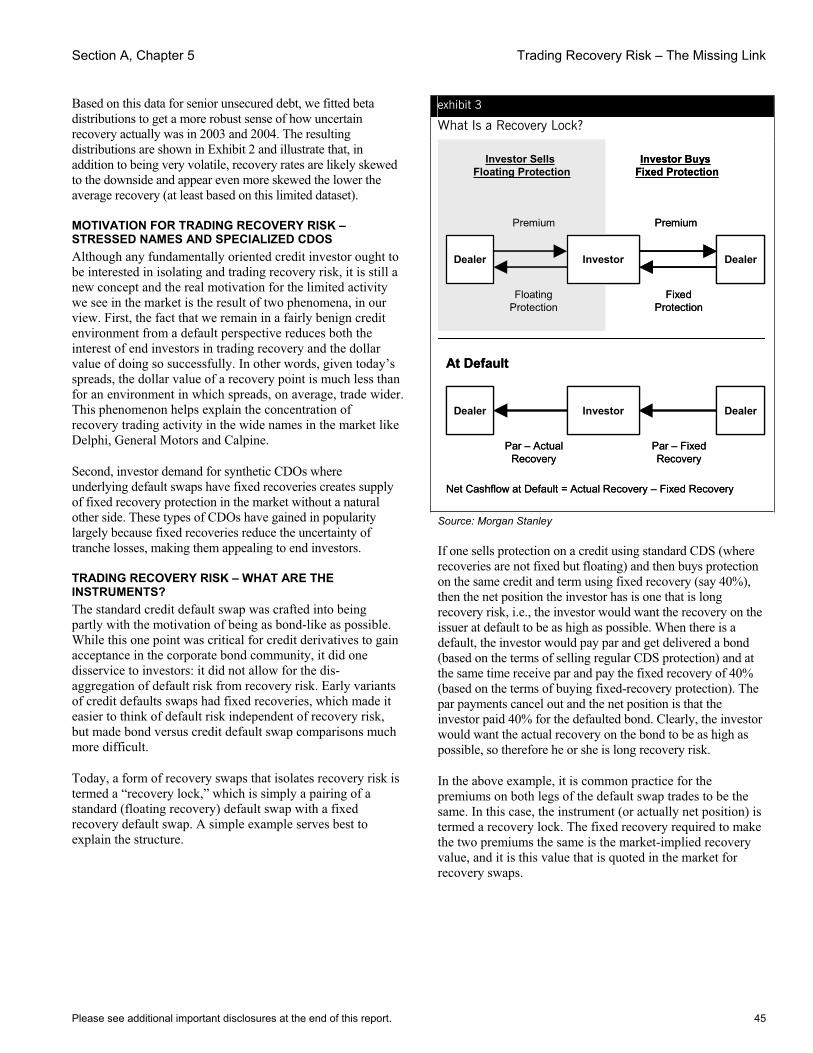
Section A, Chapter 5 Trading Recovery Risk – The Missing Link
Please see additional important disclosures at the end of this report. 45
Based on this data for senior unsecured debt, we fitted beta distributions to get a more robust sense of how uncertain recovery actually was in 2003 and 2004. The resulting distributions are shown in Exhibit 2 and illustrate that, in addition to being very volatile, recovery rates are likely skewed to the downside and appear even more skewed the lower the average recovery (at least based on this limited dataset).
MOTIVATION FOR TRADING RECOVERY RISK – STRESSED NAMES AND SPECIALIZED CDOS Although any fundamentally oriented credit investor ought to be interested in isolating and trading recovery risk, it is still a new concept and the real motivation for the limited activity we see in the market is the result of two phenomena, in our view. First, the fact that we remain in a fairly benign credit environment from a default perspective reduces both the interest of end investors in trading recovery and the dollar value of doing so successfully. In other words, given today’s spreads, the dollar value of a recovery point is much less than for an environment in which spreads, on average, trade wider. This phenomenon helps explain the concentration of recovery trading activity in the wide names in the market like Delphi, General Motors and Calpine.
Second, investor demand for synthetic CDOs where underlying default swaps have fixed recoveries creates supply of fixed recovery protection in the market without a natural other side. These types of CDOs have gained in popularity largely because fixed recoveries reduce the uncertainty of tranche losses, making them appealing to end investors.
TRADING RECOVERY RISK – WHAT ARE THE INSTRUMENTS?The standard credit default swap was crafted into being partly with the motivation of being as bond-like as possible. While this one point was critical for credit derivatives to gain acceptance in the corporate bond community, it did one disservice to investors: it did not allow for the dis-aggregation of default risk from recovery risk. Early variants of credit defaults swaps had fixed recoveries, which made it easier to think of default risk independent of recovery risk, but made bond versus credit default swap comparisons much more difficult.
Today, a form of recovery swaps that isolates recovery risk is termed a “recovery lock,” which is simply a pairing of a standard (floating recovery) default swap with a fixed recovery default swap. A simple example serves best to explain the structure.
exhibit 3
What Is a Recovery Lock?
Investor Sells Floating Protection
Investor Buys Fixed Protection
Premium Premium
FloatingProtection
FixedProtection
At Default
Par – ActualRecovery
Par – FixedRecovery
Net Cashflow at Default = Actual Recovery – Fixed Recovery
InvestorDealer Dealer
InvestorDealer Dealer
Investor Sells Floating Protection
Investor Buys Fixed Protection
Premium Premium
FloatingProtection
FixedProtection
At Default
Par – ActualRecovery
Par – FixedRecovery
Net Cashflow at Default = Actual Recovery – Fixed Recovery
InvestorDealer Dealer
InvestorDealer Dealer
Source: Morgan Stanley
If one sells protection on a credit using standard CDS (where recoveries are not fixed but floating) and then buys protection on the same credit and term using fixed recovery (say 40%), then the net position the investor has is one that is long recovery risk, i.e., the investor would want the recovery on the issuer at default to be as high as possible. When there is a default, the investor would pay par and get delivered a bond (based on the terms of selling regular CDS protection) and at the same time receive par and pay the fixed recovery of 40% (based on the terms of buying fixed-recovery protection). The par payments cancel out and the net position is that the investor paid 40% for the defaulted bond. Clearly, the investor would want the actual recovery on the bond to be as high as possible, so therefore he or she is long recovery risk.
In the above example, it is common practice for the premiums on both legs of the default swap trades to be the same. In this case, the instrument (or actually net position) is termed a recovery lock. The fixed recovery required to make the two premiums the same is the market-implied recovery value, and it is this value that is quoted in the market for recovery swaps.
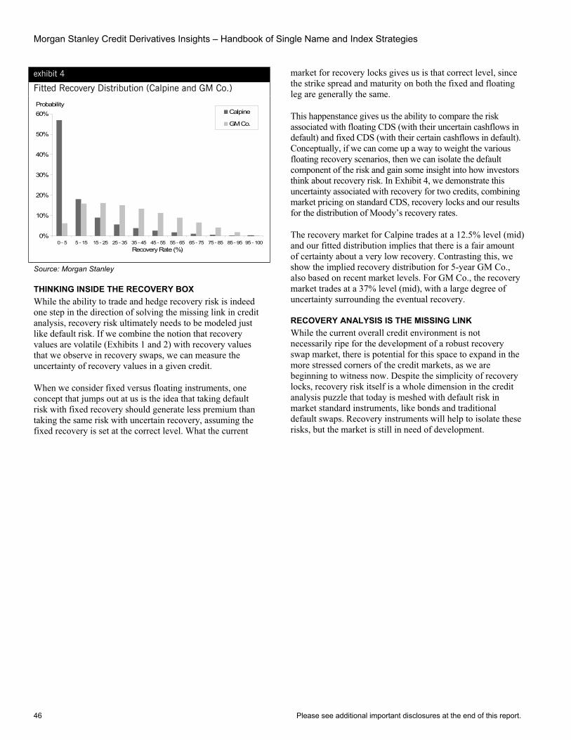
Morgan Stanley Credit Derivatives Insights – Handbook of Single Name and Index Strategies
46 Please see additional important disclosures at the end of this report.
exhibit 4
Fitted Recovery Distribution (Calpine and GM Co.)
0%
10%
20%
30%
40%
50%
60%
0 - 5 5 - 15 15 - 25 25 - 35 35 - 45 45 - 55 55 - 65 65 - 75 75 - 85 85 - 95 95 - 100Recovery Rate (%)
ProbabilityCalpine
GM Co.
Source: Morgan Stanley
THINKING INSIDE THE RECOVERY BOX While the ability to trade and hedge recovery risk is indeed one step in the direction of solving the missing link in credit analysis, recovery risk ultimately needs to be modeled just like default risk. If we combine the notion that recovery values are volatile (Exhibits 1 and 2) with recovery values that we observe in recovery swaps, we can measure the uncertainty of recovery values in a given credit.
When we consider fixed versus floating instruments, one concept that jumps out at us is the idea that taking default risk with fixed recovery should generate less premium than taking the same risk with uncertain recovery, assuming the fixed recovery is set at the correct level. What the current
market for recovery locks gives us is that correct level, since the strike spread and maturity on both the fixed and floating leg are generally the same.
This happenstance gives us the ability to compare the risk associated with floating CDS (with their uncertain cashflows in default) and fixed CDS (with their certain cashflows in default). Conceptually, if we can come up a way to weight the various floating recovery scenarios, then we can isolate the default component of the risk and gain some insight into how investors think about recovery risk. In Exhibit 4, we demonstrate this uncertainty associated with recovery for two credits, combining market pricing on standard CDS, recovery locks and our results for the distribution of Moody’s recovery rates.
The recovery market for Calpine trades at a 12.5% level (mid) and our fitted distribution implies that there is a fair amount of certainty about a very low recovery. Contrasting this, we show the implied recovery distribution for 5-year GM Co., also based on recent market levels. For GM Co., the recovery market trades at a 37% level (mid), with a large degree of uncertainty surrounding the eventual recovery.
RECOVERY ANALYSIS IS THE MISSING LINK While the current overall credit environment is not necessarily ripe for the development of a robust recovery swap market, there is potential for this space to expand in the more stressed corners of the credit markets, as we are beginning to witness now. Despite the simplicity of recovery locks, recovery risk itself is a whole dimension in the credit analysis puzzle that today is meshed with default risk in market standard instruments, like bonds and traditional default swaps. Recovery instruments will help to isolate these risks, but the market is still in need of development.
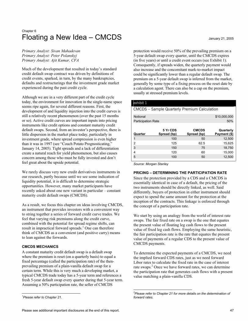
Please see additional important disclosures at the end of this report. 47
Chapter 6
Floating a New Idea – CMCDS January 21, 2005
Primary Analyst: Sivan Mahadevan Primary Analyst: Peter Polanskyj Primary Analyst: Ajit Kumar, CFA
Much of the development that resulted in today’s standard credit default swap contract was driven by definitions of credit events, sparked, in turn, by the many bankruptcies, defaults and restructurings that the investment grade market experienced during the past credit cycle.
Although we are in a very different part of the credit cycle today, the environment for innovation in the single-name space seems ripe again, for several different reasons. First, the development of and liquidity injection into the credit curves is still a relatively recent phenomenon (over the past 15 months or so). Active credit curves are important inputs into pricing instruments like credit options and constant maturity credit default swaps. Second, from an investor’s perspective, there is little dispersion in the market place today, particularly in investment grade, where spread compression is even higher than it was in 1997 (see “Couch Potato Prognosticating,” January 14, 2005). Tight spreads and a lack of differentiation create a natural reach for yield phenomenon, but also causes concern among those who must be fully invested and don’t feel great about the upside potential.
We rarely discuss very new credit derivatives instruments in our research, partly because until we see some indication of liquidity potential, it is difficult to determine strategic opportunities. However, many market participants have recently asked about one new variant in particular – constant maturity credit default swaps (CMCDS).
As a result, we focus this chapter on ideas involving CMCDS, an instrument that provides investors with a convenient way to string together a series of forward credit curve trades. We feel that varying risk premiums along the credit curve, combined with the potential for spread regime shifts, can result in impractical forward spreads.1 One can therefore think of CMCDS as a convenient (and positive carry) means to lean against the forwards.
CMCDS MECHANICS A constant maturity credit default swap is a default swap where the premium is reset (on a quarterly basis) to equal a fixed percentage (called the participation rate) of the then-prevailing premium of a plain-vanilla default swap for a certain term. While this is very much a developing market, a typical CMCDS trade today has a 5-year term and references a fresh 5-year default swap every quarter during that 5-year term. Assuming a 50% participation rate, the seller of CMCDS
1Please refer to Chapter 21.
protection would receive 50% of the prevailing premium on a 5-year default swap every quarter, until the CMCDS expires (in five years) or until a credit event occurs (see Exhibit 1). Consequently, if spreads widen, the quarterly payment would also increase and the concomitant mark-to-market impact could be significantly lower than a regular default swap. The premium on a 5-year default swap is inferred from the market, generally by some type of a fixing process on the reset date by a calculation agent. There can also be a cap on the premium, usually at stressed premium levels.
exhibit 1
CMCDS – Sample Quarterly Premium Calculation
Notional $10,000,000Participation Rate 50%
Quarter 5 Yr CDS
Spread (bp) CMCDS
Spread (bp)Quarterly
Payment ($)1 100 50 12,5002 125 62.5 15,6253 150 75 18,7504 120 60 15,0005 100 50 12,500
Source: Morgan Stanley
PRICING – DETERMINING THE PARTICIPATION RATE Since the protection provided by a CDS and a CMCDS is essentially identical in case of a default, the pricing of the two instruments should be directly linked, as well. Said differently, buyers of protection in either instrument should expect to spend the same amount for the protection at the inception of the contracts. This linkage is enforced through the concept of a participation rate.
We start by using an analogy from the world of interest rate swaps. The fair fixed rate on a swap is the one that equates the present value of floating leg cash flows to the present value of fixed leg cash flows. Employing the same heuristic, the fair participation rate is the rate that equates the present value of payments of a regular CDS to the present value of CMCDS payments.
To determine the expected payments of a CMCDS, we need the implied forward CDS rates, just as we need forward Libor rates to calculate the fixed rate in the case of interest rate swaps.2 Once we have forward rates, we can determine the participation rate that generates cash flows with a present value matching a plain-vanilla CDS.
2Please refer to Chapter 21 for more details on the determination of forward rates.
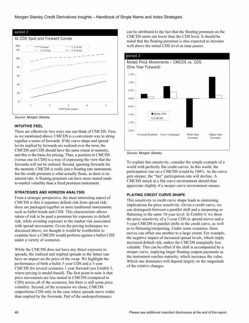
Morgan Stanley Credit Derivatives Insights – Handbook of Single Name and Index Strategies
48 Please see additional important disclosures at the end of this report.
exhibit 2
IG CDX Spot and Forward Curves
(bp)
0
20
40
60
80
100
120
1 2 3 4 5CDS Term (years)
Current 1 Yr Fwd3 Yr Fwd 5 Yr Fwd
Source: Morgan Stanley
INTUITIVE FEEL There are effectively two ways one can think of CMCDS. First, as we mentioned above, CMCDS is a convenient way to string together a series of forwards. If the curve shape and spread levels implied by forwards are realized over the term, the CMCDS and CDS should have the same return at maturity, and this is the basis for pricing. Thus, a position in CMCDS (versus one in CDS) is a way of expressing the view that the forwards will not be realized. Second, ignoring forwards for the moment, CMCDS is really just a floating rate instrument, but the credit premium is what actually floats, as there is no interest rate. A floating premium can have more muted mark-to-market volatility than a fixed premium instrument.
STRATEGIES AND HORIZON ANALYSIS From a strategic perspective, the most interesting aspect of CMCDS is that it separates default risk from spread risk; these are packaged together in more traditional instruments, such as bullet bonds and CDS. This characteristic allows takers of risk to be paid a premium for exposure to default risk, while avoiding exposure to the market risk associated with spread movements. Given the pricing techniques we discussed above, we thought it would be worthwhile to examine how a CMCDS would perform against a bullet CDS under a variety of scenarios.
While the CMCDS does not have any direct exposure to spreads, the realized and implied spreads in the future can have an impact on the price of the swap. We highlight the performance of both a bullet 5-year CDS and a 5-year CMCDS for several scenarios 1 year forward (see Exhibit 3, where pricing is model-based). The first point to note is that price movements are less muted in CMCDS (compared to CDS) across all of the scenarios, but there is still some price volatility. Second, of the scenarios we chose, CMCDS outperforms CDS only in the case where spreads move wider than implied by the forwards. Part of the underperformance
can be attributed to the fact that the floating premium on the CMCDS starts out lower than the CDS level. It should be noted that the floating premium is also expected to increase well above the initial CDS level as time passes.
exhibit 3
Muted Price Movements – CMCDS vs. CDS (One Year Forward)
-2.0%
-1.5%
-1.0%
-0.5%
0.0%
0.5%
1.0%
1.5%
Forwards Realized Curve Unchanged Wider thanForwards
Tighter thanForwards
Bullet CDS
CMCDS
Source: Morgan Stanley
To explain this sensitivity, consider the simple example of a world with perfectly flat credit curves. In this world, the participation rate on a CMCDS would be 100%. As the curve gets steeper, the “fair” participation rate will decline. A CMCDS struck in a flat curve environment should thus appreciate slightly if a steeper curve environment ensues.
PLAYING CREDIT CURVE SHAPE This sensitivity to credit curve shape leads to interesting implications for price sensitivity. Given a credit curve, we can distinguish between a parallel shift and a steepening or flattening to the same 10-year level. In Exhibit 4, we show the price sensitivity of a 5-year CDS to spread moves and a 5-year CMCDS to parallel shifts in the credit curve, as well as to flattening/steepening. Under some scenarios, these moves can offset one another to a large extent. For example, the negative impact of increased spread levels, which imply increased default risk, makes the CMCDS marginally less valuable. This can be offset if the shift is accompanied by a steeper curve, implying larger floating coupon payments as the instrument reaches maturity, which increases the value. Which one dominates will depend largely on the magnitude of the relative changes.

Section A, Chapter 6 Floating a New Idea – CMCDS
Please see additional important disclosures at the end of this report. 49
exhibit 4
CDS and CMCDS Spread and Curve Exposures(Price Sensitivity of $10MM 5 Year Positions)
-6,000 -5,000 -4,000 -3,000 -2,000 -1,000 0 1,000 2,000 3,000
5 Year Bullet DV01(Wider)
PV of Parallel 01Shift (Wider)
PV of 01 of CurveSteepness
PV of Wider Spreadwith Steepening
Bullet CDS
CMCDS
Source: Morgan Stanley
WHO ARE THE NATURAL BUYERS AND SELLERS? Right now, there are not many of either, and there may never be. Yet, as we saw above, the risk and return implications of CMCDS are significantly different from CDS in many scenarios (except when the forwards are realized) so it is indeed worth considering who might benefit from buying or selling CMCDS protection. In the current credit curve environment, the seller of protection gives up quite a bit of current premium, but could have less mark-to-market volatility and will outperform CDS when spreads go wider than implied by the forwards. For those who must be invested, but have a negative view on credit (over and above what is implied by forwards), selling CMCDS protection would be beneficial. It is also a simple way of implementing the view that default risk is benign, but spread levels are not very exciting (which fits our view, see “Breaking Down the Barriers,” December 17, 2004). Long/short strategies in tranches can also implement this view, but can be more complicated in nature.
The natural buyer of CMCDS protection is perhaps more straightforward, given that lower current premiums might seem appealing. For any protection buyer who feels that the forwards overstate spread widening over the term, buying CMCDS protection on its own would be more attractive than CDS protection itself. In either case (buyer or seller), lower potential mark-to-market volatility of CMCDS may be appealing to investors who value the lower volatility, or who must treat cash and derivative instruments differently.
SOME PRACTICAL ISSUES For investors who are excited about the convenience of packaging forwards into a single instrument, and the resulting different risk and return characteristics (compared to traditional CDS), we caution that these instruments are still relatively nascent. Transaction costs and the potential that market prices can drift away from model-based valuations are important practical implications (consider how correlation skew has moved with spread levels). Also, while the cap in CMCDS is generally deep out of the money at inception, the pricing of this cap as stress enters a particular credit can be somewhat subjective, as well.
What little activity we have seen in the market for CMCDS has been centered around the benchmark indices, rather than individual credits. One debate in the market has focused on how to treat the index roll. From a risk-management perspective, we find it simpler to think of a CMCDS on an index to always be based on today’s composition of the index; however, as indices roll and become off-the-run, it may prove difficult to apply a fixing process to levels on an off-the-run index. As a result, some market participants have proposed that, as the index rolls, the CMCDS should refer to the new index, which leaves the CMCDS users exposed to changes in index constituents. In any event, what we find interesting about this instrument is its vastly different risk and return profile, which can encourage investors to think outside of the box.
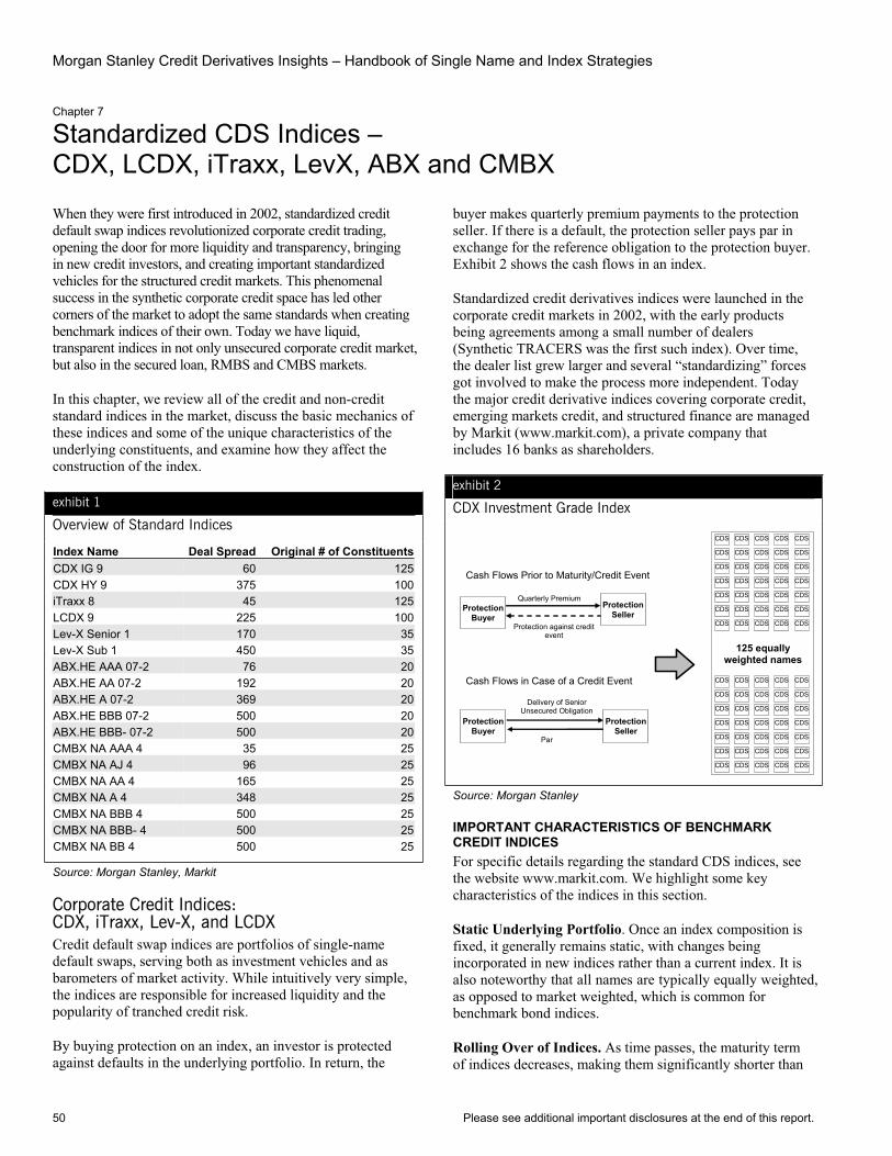
Morgan Stanley Credit Derivatives Insights – Handbook of Single Name and Index Strategies
50 Please see additional important disclosures at the end of this report.
Chapter 7
Standardized CDS Indices –CDX, LCDX, iTraxx, LevX, ABX and CMBX
When they were first introduced in 2002, standardized credit default swap indices revolutionized corporate credit trading, opening the door for more liquidity and transparency, bringing in new credit investors, and creating important standardized vehicles for the structured credit markets. This phenomenal success in the synthetic corporate credit space has led other corners of the market to adopt the same standards when creating benchmark indices of their own. Today we have liquid, transparent indices in not only unsecured corporate credit market, but also in the secured loan, RMBS and CMBS markets.
In this chapter, we review all of the credit and non-credit standard indices in the market, discuss the basic mechanics of these indices and some of the unique characteristics of the underlying constituents, and examine how they affect the construction of the index.
exhibit 1
Overview of Standard Indices
Index Name Deal Spread Original # of ConstituentsCDX IG 9 60 125CDX HY 9 375 100iTraxx 8 45 125LCDX 9 225 100Lev-X Senior 1 170 35Lev-X Sub 1 450 35ABX.HE AAA 07-2 76 20ABX.HE AA 07-2 192 20ABX.HE A 07-2 369 20ABX.HE BBB 07-2 500 20ABX.HE BBB- 07-2 500 20CMBX NA AAA 4 35 25CMBX NA AJ 4 96 25CMBX NA AA 4 165 25CMBX NA A 4 348 25CMBX NA BBB 4 500 25CMBX NA BBB- 4 500 25CMBX NA BB 4 500 25
Source: Morgan Stanley, Markit
Corporate Credit Indices: CDX, iTraxx, Lev-X, and LCDX Credit default swap indices are portfolios of single-name default swaps, serving both as investment vehicles and as barometers of market activity. While intuitively very simple, the indices are responsible for increased liquidity and the popularity of tranched credit risk.
By buying protection on an index, an investor is protected against defaults in the underlying portfolio. In return, the
buyer makes quarterly premium payments to the protection seller. If there is a default, the protection seller pays par in exchange for the reference obligation to the protection buyer. Exhibit 2 shows the cash flows in an index.
Standardized credit derivatives indices were launched in the corporate credit markets in 2002, with the early products being agreements among a small number of dealers (Synthetic TRACERS was the first such index). Over time, the dealer list grew larger and several “standardizing” forces got involved to make the process more independent. Today the major credit derivative indices covering corporate credit, emerging markets credit, and structured finance are managed by Markit (www.markit.com), a private company that includes 16 banks as shareholders.
exhibit 2
CDX Investment Grade Index
Delivery of Senior Unsecured Obligation
Par
Cash Flows in Case of a Credit Event
Protection Seller
Quarterly Premium
Protection against credit event
CDS CDS CDS CDS CDS
CDS CDS CDS CDS CDS
CDS CDS CDS CDS CDS
CDS CDS CDS CDS CDS
CDS CDS CDS CDS CDS
CDS CDS CDS CDS CDS
CDS CDS CDS CDS CDS
CDS CDS CDS CDS CDS
CDS CDS CDS CDS CDS
CDS CDS CDS CDS CDS
CDS CDS CDS CDS CDS
CDS CDS CDS CDS CDS
CDS CDS CDS CDS CDS
CDS CDS CDS CDS CDS
125 equally weighted names
Protection Buyer
Protection Buyer
Protection Seller
Cash Flows Prior to Maturity/Credit Event
Source: Morgan Stanley
IMPORTANT CHARACTERISTICS OF BENCHMARK CREDIT INDICES For specific details regarding the standard CDS indices, see the website www.markit.com. We highlight some key characteristics of the indices in this section.
Static Underlying Portfolio. Once an index composition is fixed, it generally remains static, with changes being incorporated in new indices rather than a current index. It is also noteworthy that all names are typically equally weighted, as opposed to market weighted, which is common for benchmark bond indices.
Rolling Over of Indices. As time passes, the maturity term of indices decreases, making them significantly shorter than
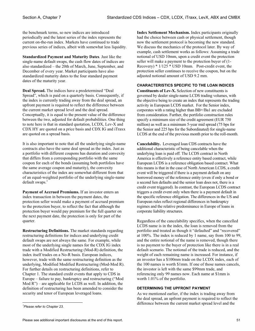
Section A, Chapter 7 Standardized CDS Indices – CDX, LCDX, iTraxx, LevX, ABX and CMBX
Please see additional important disclosures at the end of this report. 51
the benchmark terms, so new indices are introduced periodically and the latest series of the index represents the current on-the-run index. Markets have continued to trade previous series of indices, albeit with somewhat less liquidity.
Standardized Payment and Maturity Dates. Just like the single-name default swaps, the cash flow dates of indices are also standardized – the 20th of March, June, September, and December of every year. Market participants have also standardized maturity dates to the four standard payment dates of the maturity year.
Deal Spread. The indices have a predetermined “Deal Spread”, which is paid on a quarterly basis. Consequently, if the index is currently trading away from the deal spread, an upfront payment is required to reflect the difference between the current market spread level and the deal spread. Conceptually, it is equal to the present value of the difference between the two, adjusted for default probabilities. One thing to note here is that in standard quotation, LCDX, Lev-X and CDX HY are quoted on a price basis and CDX IG and iTraxx are quoted on a spread basis.
It is also important to note that all the underlying single-name contracts also have the same deal spread as the index. Just as a portfolio with different coupons has duration and convexity that differs from a corresponding portfolio with the same coupon for each of the bonds (assuming both portfolios have the same average coupon and maturity), the convexity characteristics of the index are somewhat different from that of an equal-weighted portfolio of the underlying single-name default swaps.1
Payment of Accrued Premiums. If an investor enters an index transaction in between the payment dates, the protection seller would make a payment of accrued premium to the protection buyer, to reflect the fact that although the protection buyer would pay premium for the full quarter on the next payment date, the protection is only for part of the quarter.
Restructuring Definitions. The market standards regarding restructuring definitions for indices and underlying credit default swaps are not always the same. For example, while most of the underlying single names for the CDX IG index trade with a Modified Restructuring (Mod-R) definition, the index itself trades on a No-R basis. European indices, however, trade with the same restructuring definition as the underlying, Modified Modified Restructuring (Mod-Mod R). For further details on restructuring definitions, refer to Chapter 1. The standard credit events that apply to CDS in Europe – failure to pay, bankruptcy and restructuring (“Mod Mod R”) – are applicable for LCDS as well. In addition, the definition of restructuring has been amended to consider the security and tenor of European leveraged loans.
1Please refer to Chapter 23.
Index Settlement Mechanism. Index participants originally had the choice between cash or physical settlement, though now the settlement protocol is becoming the new standard. We discuss the mechanics of the protocol later. By way of example, cash settlement works as follows: Assuming a trade notional of USD 10mm, upon a credit event the protection seller will make a payment to the protection buyer of (1-Recovery) * 1/125 * USD 10mm. Post-credit event, the protection seller continues to receive the coupon, but on the adjusted notional amount of USD 9.2 mm.
CHARACTERISTICS SPECIFIC TO THE LOAN INDICES Constituents of Lev-X. Selection of new constituents is governed by dealer single-name LCDS trading volumes, with the objective being to create an index that represents the trading activity in European LCDS market. For the Senior index, corporates with a rating higher than BB+/Ba1 are excluded from consideration. Further, the portfolio construction rules specify a minimum size of the credit agreement (EUR 750 million) as well as a minimum 5-year mid spread (75 bps for the Senior and 225 bps for the Subordinated) for single-name LCDS at the end of the previous month prior to the roll-month.
Cancelability. Leveraged loan CDS contracts have the additional characteristic of being cancelable when the underlying loan is paid off. The LCDS contract in North America is effectively a reference entity based contract, while European LCDS is a reference obligation based contract. What this means is that in the case of North American LCDS, a credit event will be triggered if there is a payment default on any borrowed money of the reference entity (even if only a bond or a second lien defaults and the senior loan does not, there is a credit event triggered). In contrast, the European LCDS contract triggers a credit event only when there is a payment default in the specific reference obligation. The differences in the US and European rules reflect regional differences in bankruptcy regimes and the relative predominance in Europe of loans in corporate liability structures.
Regardless of the cancelability specifics, when the cancelled LCDS name is in the index, the loan is removed from the portfolio and treated as though it “defaulted” and “recovered” at 100%. The index is reduced by 1 name, say from 100 to 99, and the entire notional of the name is removed, though there is no payment to the buyer of protection like there is in a real default scenario. The notional of the trade is reduced, and the weight of each remaining name is increased. For instance, if an investor has a $100mm trade on the LCDX index, each of the 100 names is worth $1mm. If one of those names cancels, the investor is left with the same $99mm trade, and referencing only 99 names now. Each name at $1mm is worth 1.01% of the portfolio.
DETERMINING THE UPFRONT PAYMENT As we mentioned earlier, if the index is trading away from the deal spread, an upfront payment is required to reflect the difference between the current market spread level and the
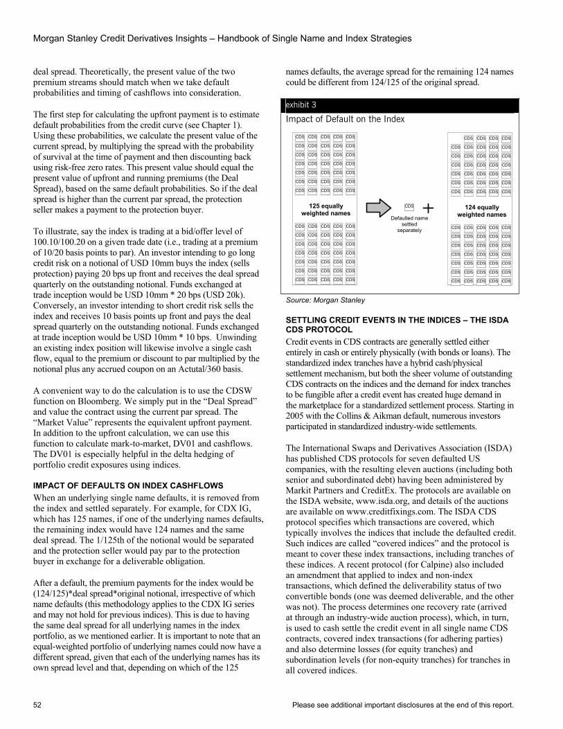
Morgan Stanley Credit Derivatives Insights – Handbook of Single Name and Index Strategies
52 Please see additional important disclosures at the end of this report.
deal spread. Theoretically, the present value of the two premium streams should match when we take default probabilities and timing of cashflows into consideration.
The first step for calculating the upfront payment is to estimate default probabilities from the credit curve (see Chapter 1). Using these probabilities, we calculate the present value of the current spread, by multiplying the spread with the probability of survival at the time of payment and then discounting back using risk-free zero rates. This present value should equal the present value of upfront and running premiums (the Deal Spread), based on the same default probabilities. So if the deal spread is higher than the current par spread, the protection seller makes a payment to the protection buyer.
To illustrate, say the index is trading at a bid/offer level of 100.10/100.20 on a given trade date (i.e., trading at a premium of 10/20 basis points to par). An investor intending to go long credit risk on a notional of USD 10mm buys the index (sells protection) paying 20 bps up front and receives the deal spread quarterly on the outstanding notional. Funds exchanged at trade inception would be USD 10mm * 20 bps (USD 20k). Conversely, an investor intending to short credit risk sells the index and receives 10 basis points up front and pays the deal spread quarterly on the outstanding notional. Funds exchanged at trade inception would be USD 10mm * 10 bps. Unwinding an existing index position will likewise involve a single cash flow, equal to the premium or discount to par multiplied by the notional plus any accrued coupon on an Actutal/360 basis.
A convenient way to do the calculation is to use the CDSW function on Bloomberg. We simply put in the “Deal Spread” and value the contract using the current par spread. The “Market Value” represents the equivalent upfront payment. In addition to the upfront calculation, we can use this function to calculate mark-to-market, DV01 and cashflows. The DV01 is especially helpful in the delta hedging of portfolio credit exposures using indices.
IMPACT OF DEFAULTS ON INDEX CASHFLOWS When an underlying single name defaults, it is removed from the index and settled separately. For example, for CDX IG, which has 125 names, if one of the underlying names defaults, the remaining index would have 124 names and the same deal spread. The 1/125th of the notional would be separated and the protection seller would pay par to the protection buyer in exchange for a deliverable obligation.
After a default, the premium payments for the index would be (124/125)*deal spread*original notional, irrespective of which name defaults (this methodology applies to the CDX IG series and may not hold for previous indices). This is due to having the same deal spread for all underlying names in the index portfolio, as we mentioned earlier. It is important to note that an equal-weighted portfolio of underlying names could now have a different spread, given that each of the underlying names has its own spread level and that, depending on which of the 125
names defaults, the average spread for the remaining 124 names could be different from 124/125 of the original spread.
exhibit 3
Impact of Default on the Index
CDS
CDS CDS CDS CDS
CDS CDS CDS CDS CDS
CDS CDS CDS CDS CDS
CDS CDS CDS CDS CDS
CDS CDS CDS CDS CDS
CDS CDS CDS CDS CDS
CDS CDS CDS CDS CDS
CDS CDS CDS CDS CDS
CDS CDS CDS CDS CDS
CDS CDS CDS CDS CDS
CDS CDS CDS CDS CDS
CDS CDS CDS CDS CDS
CDS CDS CDS CDS CDS
CDS CDS CDS CDS CDS
124 equally weighted names
CDS CDS CDS CDS CDS
CDS CDS CDS CDS CDS
CDS CDS CDS CDS CDS
CDS CDS CDS CDS CDS
CDS CDS CDS CDS CDS
CDS CDS CDS CDS CDS
CDS CDS CDS CDS CDS
CDS CDS CDS CDS CDS
CDS CDS CDS CDS CDS
CDS CDS CDS CDS CDS
CDS CDS CDS CDS CDS
CDS CDS CDS CDS CDS
CDS CDS CDS CDS CDS
CDS CDS CDS CDS CDS
125 equally weighted names
Defaulted name settled
separately
Source: Morgan Stanley
SETTLING CREDIT EVENTS IN THE INDICES – THE ISDA CDS PROTOCOL Credit events in CDS contracts are generally settled either entirely in cash or entirely physically (with bonds or loans). The standardized index tranches have a hybrid cash/physical settlement mechanism, but both the sheer volume of outstanding CDS contracts on the indices and the demand for index tranches to be fungible after a credit event has created huge demand in the marketplace for a standardized settlement process. Starting in 2005 with the Collins & Aikman default, numerous investors participated in standardized industry-wide settlements.
The International Swaps and Derivatives Association (ISDA) has published CDS protocols for seven defaulted US companies, with the resulting eleven auctions (including both senior and subordinated debt) having been administered by Markit Partners and CreditEx. The protocols are available on the ISDA website, www.isda.org, and details of the auctions are available on www.creditfixings.com. The ISDA CDS protocol specifies which transactions are covered, which typically involves the indices that include the defaulted credit. Such indices are called “covered indices” and the protocol is meant to cover these index transactions, including tranches of these indices. A recent protocol (for Calpine) also included an amendment that applied to index and non-index transactions, which defined the deliverability status of two convertible bonds (one was deemed deliverable, and the other was not). The process determines one recovery rate (arrived at through an industry-wide auction process), which, in turn, is used to cash settle the credit event in all single name CDS contracts, covered index transactions (for adhering parties) and also determine losses (for equity tranches) and subordination levels (for non-equity tranches) for tranches in all covered indices.
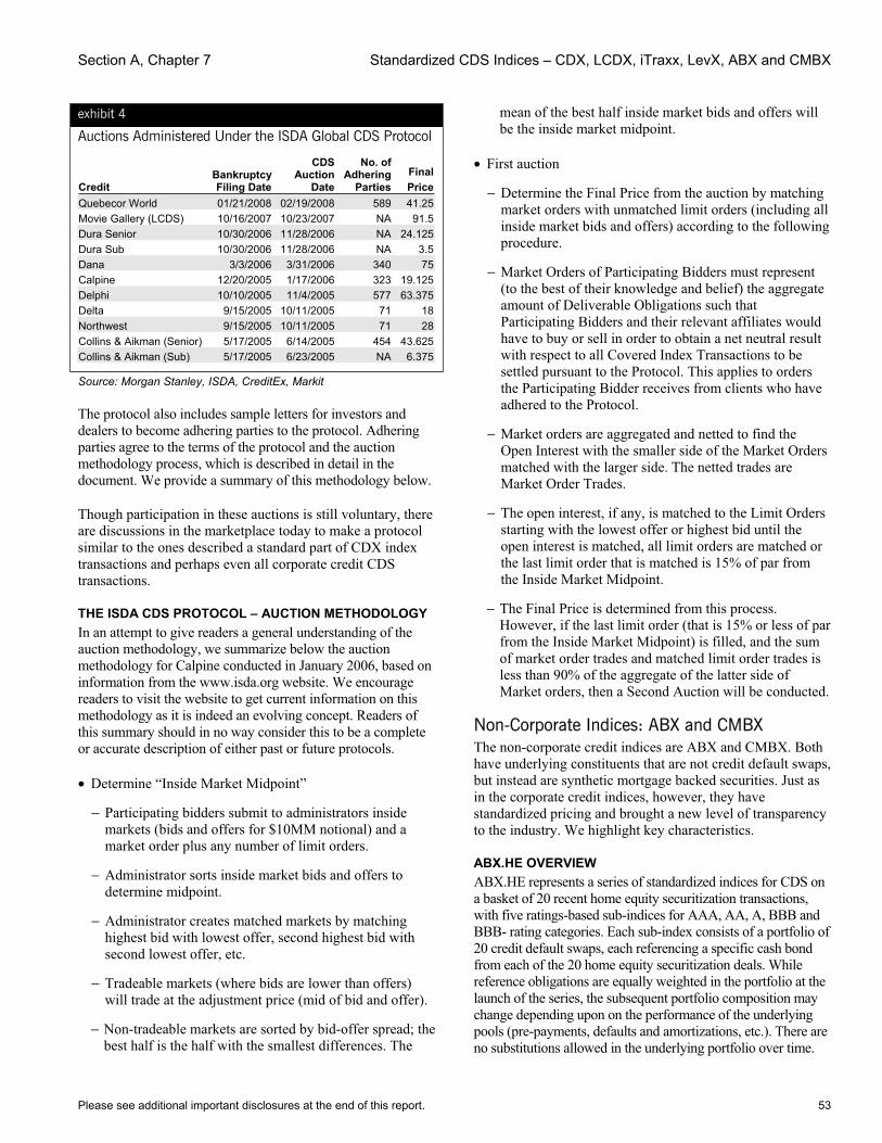
Section A, Chapter 7 Standardized CDS Indices – CDX, LCDX, iTraxx, LevX, ABX and CMBX
Please see additional important disclosures at the end of this report. 53
exhibit 4
Auctions Administered Under the ISDA Global CDS Protocol
Credit Bankruptcy Filing Date
CDSAuction
Date
No. of Adhering
PartiesFinalPrice
Quebecor World 01/21/2008 02/19/2008 589 41.25Movie Gallery (LCDS) 10/16/2007 10/23/2007 NA 91.5Dura Senior 10/30/2006 11/28/2006 NA 24.125Dura Sub 10/30/2006 11/28/2006 NA 3.5Dana 3/3/2006 3/31/2006 340 75Calpine 12/20/2005 1/17/2006 323 19.125Delphi 10/10/2005 11/4/2005 577 63.375Delta 9/15/2005 10/11/2005 71 18Northwest 9/15/2005 10/11/2005 71 28Collins & Aikman (Senior) 5/17/2005 6/14/2005 454 43.625Collins & Aikman (Sub) 5/17/2005 6/23/2005 NA 6.375
Source: Morgan Stanley, ISDA, CreditEx, Markit
The protocol also includes sample letters for investors and dealers to become adhering parties to the protocol. Adhering parties agree to the terms of the protocol and the auction methodology process, which is described in detail in the document. We provide a summary of this methodology below.
Though participation in these auctions is still voluntary, there are discussions in the marketplace today to make a protocol similar to the ones described a standard part of CDX index transactions and perhaps even all corporate credit CDS transactions.
THE ISDA CDS PROTOCOL – AUCTION METHODOLOGY In an attempt to give readers a general understanding of the auction methodology, we summarize below the auction methodology for Calpine conducted in January 2006, based on information from the www.isda.org website. We encourage readers to visit the website to get current information on this methodology as it is indeed an evolving concept. Readers of this summary should in no way consider this to be a complete or accurate description of either past or future protocols.
• Determine “Inside Market Midpoint”
− Participating bidders submit to administrators inside markets (bids and offers for $10MM notional) and a market order plus any number of limit orders.
− Administrator sorts inside market bids and offers to determine midpoint.
− Administrator creates matched markets by matching highest bid with lowest offer, second highest bid with second lowest offer, etc.
− Tradeable markets (where bids are lower than offers) will trade at the adjustment price (mid of bid and offer).
− Non-tradeable markets are sorted by bid-offer spread; the best half is the half with the smallest differences. The
mean of the best half inside market bids and offers will be the inside market midpoint.
• First auction
− Determine the Final Price from the auction by matching market orders with unmatched limit orders (including all inside market bids and offers) according to the following procedure.
− Market Orders of Participating Bidders must represent (to the best of their knowledge and belief) the aggregate amount of Deliverable Obligations such that Participating Bidders and their relevant affiliates would have to buy or sell in order to obtain a net neutral result with respect to all Covered Index Transactions to be settled pursuant to the Protocol. This applies to orders the Participating Bidder receives from clients who have adhered to the Protocol.
− Market orders are aggregated and netted to find the Open Interest with the smaller side of the Market Orders matched with the larger side. The netted trades are Market Order Trades.
− The open interest, if any, is matched to the Limit Orders starting with the lowest offer or highest bid until the open interest is matched, all limit orders are matched or the last limit order that is matched is 15% of par from the Inside Market Midpoint.
− The Final Price is determined from this process. However, if the last limit order (that is 15% or less of par from the Inside Market Midpoint) is filled, and the sum of market order trades and matched limit order trades is less than 90% of the aggregate of the latter side of Market orders, then a Second Auction will be conducted.
Non-Corporate Indices: ABX and CMBX The non-corporate credit indices are ABX and CMBX. Both have underlying constituents that are not credit default swaps, but instead are synthetic mortgage backed securities. Just as in the corporate credit indices, however, they have standardized pricing and brought a new level of transparency to the industry. We highlight key characteristics.
ABX.HE OVERVIEW ABX.HE represents a series of standardized indices for CDS on a basket of 20 recent home equity securitization transactions, with five ratings-based sub-indices for AAA, AA, A, BBB and BBB- rating categories. Each sub-index consists of a portfolio of 20 credit default swaps, each referencing a specific cash bond from each of the 20 home equity securitization deals. While reference obligations are equally weighted in the portfolio at the launch of the series, the subsequent portfolio composition may change depending upon on the performance of the underlying pools (pre-payments, defaults and amortizations, etc.). There are no substitutions allowed in the underlying portfolio over time.

Morgan Stanley Credit Derivatives Insights – Handbook of Single Name and Index Strategies
54 Please see additional important disclosures at the end of this report.
DIFFERENCES BETWEEN ABX.HE AND SF CDS The mechanics of the ABX.HE are similar to single-name SF CDS with a few important exceptions. First, while the single-name SF CDS documentation provides for alternative mechanisms for dealing with shortfalls (fixed cap, variable cap and no cap alternatives as described earlier), CDS referencing the ABX.HE will only have a fixed cap convention. Second, the pay-as-you-go mechanism applies but without the option for physical settlement if there is a credit event. Third, the treatment of the clean-up call is different. SF CDS contracts provide for optional termination of the CDS if the underlying transaction is not called, and if the CDS remains in effect, the premium usually steps up. With the ABX.HE, there is no optional termination provision when a clean-up call is not exercised and there is no step-up in premium.
ABX.HE MECHANICS Consistent with the pay-as-you-go approach, the obligation of the protection seller is to cover interest shortfall amounts up to the premium payments and any principal shortfall and writedown amounts of the reference obligations in the portfolio. Without the optional physical settlement provision, the maturity of the ABX.HE is effectively the maturity of the longest CDS within the underlying portfolio. The payments from the buyer and seller of protection are summarized in Exhibit 5 below.
exhibit 5
Payments by Protection Buyers and Sellers on ABX.HE
Protection Buyer (Fixed Rate Payer)
Protection Seller (Floating Rate Payer)
Pays a monthly premium (quoted as basis points per annum) to the protection seller on notional amount• The notional amount will decline
over time based on the reference obligation amortization and any principal writedown
Receives a monthly premium (quoted as basis points per annum) from the protection buyer on notional amount • The notional amount will decline
over time based on the reference obligation amortization and principal writedown
Receives payments from the protection seller in the event of the following • Interest shortfall (capped at the
fixed rate) • Principal shortfall • Writedown
Pays the protection buyer in the event of the following • Interest shortfall (capped at the
fixed rate) • Principal shortfall • Writedown
Pays to the protection seller in the event of the following • Interest shortfall reimbursement
amount• Principal shortfall reimbursement
amount• Writedown reimbursement amount
Receives from the protection buyer in the event of the following • Interest shortfall reimbursement
amount• Principal shortfall reimbursement
amount• Writedown reimbursement amount
Source: Morgan Stanley
To further illustrate the changes to the notional amount and payments in the event of a writedown, consider the following scenario. Say the fixed rate paid by the protection buyer on a notional of $100 million is 70 bps; at index inception the factor on the reference obligation was 1.0 and is now 0.75; and a writedown in the amount of 1% of the current principal balance
occurs in year 3. The writedown amount is calculated as the product of (current factor * weighting of the reference obligation in the index * the writedown %) and the notional amount. In our example, this equals $37,500 = (0.75 * 0.05 * 0.01) * $100 mm. The index notional amount will be reduced by 0.0375% and subsequent fixed payments (70 bp) by the protection buyer will be on the remaining index notional amount.
ABX.HE TRADES ON PRICE NOT SPREAD Since there are no standard prepayment conventions, and since different investors make different prepayment assumptions resulting in different durations for the underlying reference obligations, trading the indices on spread terms can be complicated. Consequently, the ABX.HE indices trade on price terms. Each index has a predetermined premium that is fixed (as a percentage of notional) over the life of the index. Index prices will be quoted in a typical bond convention, as a percentage of par and any premium or discount is exchanged upfront. To illustrate this, assume that the index is at 100 and the index fixed rate is the market spread. If on a subsequent trade date the index is at 98, it means that the implied spreads have widened. For a trade initiated that day, the protection buyer pays the protection seller 2% * notional * current factor. On the other hand, if on that trade date, the index is at 102, it means that the implied spreads have tightened and the protection seller pays the protection buyer 2% * notional * current factor.
ABX.HE: PORTFOLIO CONSTRUCTION2
The portfolio of reference obligations for each ABX.HE series will be constructed such that the index is representative of the sub-prime home equity market. The third-party administrator will submit to each participating dealer two deals from the largest 25 sub-prime home equity bond issuers based on the following criterion:
(a) Issued within the previous six months.
(b) Minimum issue offering size of $500 million.
(c) At least 90% of the deal’s assets must be first lien mortgages.
(d) Weighted average FICO score of the borrowers in the pool < 660
(e) Referenced tranches must be floating rate payers indexed to one-month LIBOR
(f) At issuance, each deal must have tranches with ratings of each of the sub-indices with an average life greater than four years, except for the AAA tranche which must have an average life greater than five years
(g) All tranches rated by both S&P and Moody’s – if split rated, the lower rating will apply
2This section is largely drawn from the ABX Rules, January 17, 2006, available at http://www.markit.com/abx.jsp
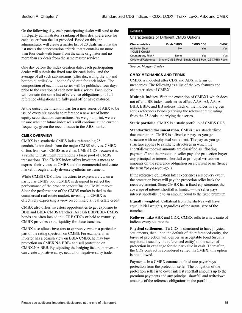
Section A, Chapter 7 Standardized CDS Indices – CDX, LCDX, iTraxx, LevX, ABX and CMBX
Please see additional important disclosures at the end of this report. 55
On the following day, each participating dealer will send to the third-party administrator a ranking of their deal preference for each issuer from the list provided. Based on this, the administrator will create a master list of 20 deals such that the list meets the concentration criteria that it contains no more than four deals with loans from the same originator and no more than six deals from the same master servicer.
One day before the index creation date, each participating dealer will submit the fixed rate for each index, and the average of all such submissions (after discarding the top and bottom quartiles) will be the fixed rate for each index. The composition of each index series will be published four days prior to the creation of each new index series. Each index will contain the same list of reference obligations until all reference obligations are fully paid off or have matured.
At the outset, the intention was for a new series of ABX to be issued every six months to reference a new set of home equity securitization transactions. As we go to print, we are unsure whether future index rolls will continue at the current frequency, given the recent issues in the ABS market.
CMBX OVERVIEW CMBX is a synthetic CMBS index referencing 25 conduit/fusion deals from the major CMBS shelves. CMBX differs from cash CMBS as well as CMBS CDS because it is a synthetic instrument referencing a large pool of CMBS transactions. The CMBX index offers investors a means to express their views on CMBS and the commercial real estate market through a fairly diverse synthetic instrument.
While CMBS CDS allow investors to express a view on a particular CMBS pool, CMBX is designed to reflect the performance of the broader conduit/fusion CMBS market. Since the performance of the CMBS market is tied to the commercial real estate market, investing in CMBX is effectively expressing a view on commercial real estate credit.
CMBX also offers investors opportunities to get exposure to BBB and BBB- CMBS tranches. As cash BBB/BBB- CMBS bonds are often locked into CRE CDOs or held to maturity, CMBX provides extra liquidity for these tranches.
CMBX also allows investors to express views on a particular part of the rating spectrum on CMBS. For example, if an investor has a bearish view on BBB- CMBS, he may buy protection on CMBX.NA.BBB- and sell protection on CMBX.NA.BBB. By adjusting the hedging factor, an investor can create a positive-carry, neutral, or negative-carry trade.
exhibit 6
Characteristics of Different CMBS Options
Characteristics Cash CMBS CMBS CDS CMBX Ability to Short
CMBS Credit? No Yes Yes
Counterparty Risk? None Yes Yes Collateral/Reference Single CMBS Pool Single CMBS Pool 25 CMBS Pools
Source: Morgan Stanley
CMBX MECHANICS AND TERMS CMBX is modeled after CDX and ABX in terms of mechanics. The following is a list of the key features and characteristics of CMBX.
Multiple Indices. With the exception of CMBX1 which does not offer a BB index, each series offers AAA, AJ, AA, A, BBB, BBB-, and BB indices. Each of the indices in a given series references bonds (carrying the relevant credit rating) from the 25 deals underlying that series.
Static portfolio. CMBX is a static portfolio of CMBS CDS.
Standardized documentation. CMBX uses standardized documentation. CMBX is a fixed-cap pay-as-you-go structure with no physical settlement. The pay-as-you-go structure applies to synthetic structures in which the shortfall/writedown amounts are classified as “floating payments” and the protection seller pays the protection buyer any principal or interest shortfall or principal writedown amounts on the reference obligation on a current basis (hence the term “pay-as-you-go”).
If the reference obligation later experiences a recovery event, the protection buyer will pay the protection seller back the recovery amount. Since CMBX has a fixed-cap structure, the coverage of interest shortfall is limited — the seller pays interest shortfalls up to an amount equal to the fixed premium.
Equally weighted. Collateral from the shelves will have equal initial weights, regardless of the actual size of the tranches.
Rollover. Like ABX and CDX, CMBX rolls to a new suite of indices every six months.
Physical settlement. If a CDS is structured to have physical settlements, then upon the default of the referenced entity, the buyer of protection will deliver an acceptable bond (usually any bond issued by the referenced entity) to the seller of protection in exchange for the par value in cash. Thereafter, the CDS contract is considered settled. In CMBX, this option is not allowed.
Payments. In a CMBX contract, a fixed rate payer buys protection from the protection seller. The obligation of the protection seller is to cover interest shortfall amounts up to the premium payments and any principal shortfall and writedown amounts of the reference obligations in the portfolio
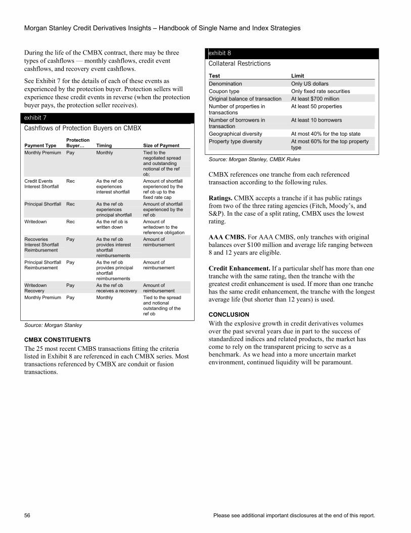
Morgan Stanley Credit Derivatives Insights – Handbook of Single Name and Index Strategies
56 Please see additional important disclosures at the end of this report.
During the life of the CMBX contract, there may be three types of cashflows — monthly cashflows, credit event cashflows, and recovery event cashflows.
See Exhibit 7 for the details of each of these events as experienced by the protection buyer. Protection sellers will experience these credit events in reverse (when the protection buyer pays, the protection seller receives).
exhibit 7
Cashflows of Protection Buyers on CMBX
Payment Type Protection Buyer… Timing Size of Payment
Monthly Premium Pay Monthly Tied to the negotiated spread and outstanding notional of the ref ob;
Credit Events Interest Shortfall
Rec As the ref ob experiences interest shortfall
Amount of shortfall experienced by the ref ob up to the fixed rate cap
Principal Shortfall Rec As the ref ob experiences principal shortfall
Amount of shortfall experienced by the ref ob
Writedown Rec As the ref ob is written down
Amount of writedown to the reference obligation
Recoveries Interest Shortfall Reimbursement
Pay As the ref ob provides interest shortfall reimbursements
Amount of reimbursement
Principal Shortfall Reimbursement
Pay As the ref ob provides principal shortfall reimbursements
Amount of reimbursement
Writedown Recovery
Pay As the ref ob receives a recovery
Amount of reimbursement
Monthly Premium Pay Monthly Tied to the spread and notional outstanding of the ref ob
Source: Morgan Stanley
CMBX CONSTITUENTS The 25 most recent CMBS transactions fitting the criteria listed in Exhibit 8 are referenced in each CMBX series. Most transactions referenced by CMBX are conduit or fusion transactions.
exhibit 8
Collateral Restrictions
Test Limit Denomination Only US dollars Coupon type Only fixed rate securities Original balance of transaction At least $700 million Number of properties in transactions
At least 50 properties
Number of borrowers in transaction
At least 10 borrowers
Geographical diversity At most 40% for the top state Property type diversity At most 60% for the top property
type
Source: Morgan Stanley, CMBX Rules
CMBX references one tranche from each referenced transaction according to the following rules.
Ratings. CMBX accepts a tranche if it has public ratings from two of the three rating agencies (Fitch, Moody’s, and S&P). In the case of a split rating, CMBX uses the lowest rating.
AAA CMBS. For AAA CMBS, only tranches with original balances over $100 million and average life ranging between 8 and 12 years are eligible.
Credit Enhancement. If a particular shelf has more than one tranche with the same rating, then the tranche with the greatest credit enhancement is used. If more than one tranche has the same credit enhancement, the tranche with the longest average life (but shorter than 12 years) is used.
CONCLUSIONWith the explosive growth in credit derivatives volumes over the past several years due in part to the success of standardized indices and related products, the market has come to rely on the transparent pricing to serve as a benchmark. As we head into a more uncertain market environment, continued liquidity will be paramount.
Please see additional important disclosures at the end of this report. 57
Chapter 8
Succeeding in an Activist World –Succession Language February 10, 2006
Primary Analyst: Sivan Mahadevan Primary Analyst: Peter Polanskyj Primary Analyst: Pinar Onur
As the volume of corporate actions rapidly increases, bankers, private equity and hedge funds spend much of their time poring over thick financial statements in search of the optimal debt capital structure for the various entities involved. One large document they are most likely not reading is the 2003 ISDA Credit Derivatives Definitions. This nearly 100-page tome is what governs most corporate credit CDS transactions today. Successor language has important implications for what obligations are deliverable into CDS following a series of corporate actions. From the perspective of sponsors, this language is arbitrary, but from the perspective of credit markets, it is immensely important as it defines what direction (or directions) CDS can take, which, in many cases, can be quite different from the direction of any given debt obligation.
We provide an interpretation of successor language in the 2003 ISDA definitions and focus on how corporate actions can potentially push CDS in different directions relative to debt obligations. There are a few rules of thumb that we can deduce from the 2003 ISDA definitions; but the devil is in the details, as there are numerous corporate situations where the timing of debt exchanges and the ultimate par value of debt that moves between entities determines successor behavior in CDS. We would also like to quell a common myth. Market participants often say that many events can result in CDS either terminating or being worthless. However, both of these situations are rare, and we offer up some examples.
WHERE DOES CDS GO? RULES OF THUMB For credit investors, we provide some basic rules of thumb regarding the impact of succession events (or the lack thereof) on CDS contracts, based on the 2003 ISDA definitions.
• When there are corporate successions, CDS contracts follow the debt of a company, rather than equity value, revenues or corporate structure. A corporate succession must result in a “Succession Event,” under the 2003 ISDA definitions, for CDS to change, although CDS can be implicitly impacted without such an event.
• The key difference between bonds and CDS in the event of succession is that CDS can be formulaically split, while bonds, by definition, have to go one direction or another (or get taken out).
• Contrary to popular belief, it is rare for CDS to be terminated as a result of corporate succession. The only
situation where it can happen is where the party to the corporate action is also the protection seller, in which case a “Termination Event” occurs. Even then, it results in a mark-to-market unwind at the option of the protection buyer.
• A debt exchange that is not in connection with a merger (or other terms of a “Succession Event”) will not qualify as a “Succession Event.” As such, there could be situations where no obligations are left to be deliverable into the CDS, although debt issued in the future could be.
• One company guaranteeing the debt of another company (say, after buying its stock) does not qualify as a “Succession Event.” If the debt is assumed by the parent company and released by the original obligor, then it is a “Succession Event.”
DEFINING SUCCESSION For bond purposes, succession really has more to do with making the credit risk of the instruments of one issuer economically similar to the instruments of another issuer. For CDS contracts, succession is a legal term with a very specific definition (from 2003 ISDA Credit Derivatives Definitions):
“Succession Event” means an event such as a merger, consolidation, amalgamation, transfer of assets or liabilities, demerger, spin-off or other similar event in which one entity succeeds to the obligations of another entity, whether by operation of law or pursuant to any agreement. Notwithstanding the foregoing, “Succession Event” shall not include an event in which the holders of obligations of the Reference Entity exchange such obligations for the obligations of another entity, unless such exchange occurs in connection with a merger, consolidation, amalgamation, transfer of assets or liabilities, demerger, spin-off or other similar event.
The definition, it would seem, is intended to capture most merger and acquisition activity, but because of the exchange exclusion, the actual timing of events can affect whether they qualify as successor events. For example, does an exchange offer that occurs several weeks or months subsequent to a merger automatically qualify as being “in connection” with the merger? It seems reasonable that interpretations could differ.
THE MATH BEHIND SUCCESSORS AND CDS Once we have defined whether an event is a successor event, we next need to consider how various instruments react. For cash bonds and loans, generally, the corporation will specify the intention to either buy back debt and have it assumed by the new entity or any other action, which may or may not be subject to approval by bondholders. So the fate of any individual bond is fairly clear.
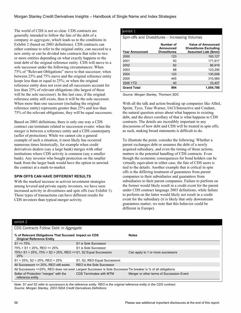
Morgan Stanley Credit Derivatives Insights – Handbook of Single Name and Index Strategies
58 Please see additional important disclosures at the end of this report.
The world of CDS is not so clear. CDS contracts are generally intended to follow the fate of the debt of a company in aggregate, which leads us to the conditions in Exhibit 2 (based on 2003 definitions). CDS contracts can either continue to refer to the original entity, can succeed to a new entity or can be divided into contracts that refer to two or more entities depending on what exactly happens to the total debt of the original reference entity. CDS will move to a sole successor under the following circumstances: When 75% of “Relevant Obligations” move to that successor; when between 25% and 75% move and the original reference entity keeps less than or equal to 25%; or when the original reference entity does not exist and all successors account for less than 25% of relevant obligations (the largest of these will be the sole successor). In this last case, if the original reference entity still exists, then it will be the sole successor. When more than one successor (including the original reference entity) represents greater than 25% and less than 75% of the relevant obligations, they will be equal successors.
Based on 2003 definitions, there is only one way a CDS contract can terminate related to succession events: when the merger is between a reference entity and a CDS counterparty (seller of protection). While we cannot cite a general example of such a situation, it most likely has occurred numerous times historically, for example when credit derivatives dealers (say a large bank) merges with other institutions where CDS activity is common (say a smaller bank). Any investor who bought protection on the smaller bank from the larger bank would have the option to unwind the contract at a mark-to-market.
SPIN OFFS CAN HAVE DIFFERENT RESULTS With the marked increase in activist investment strategies among levered and private equity investors, we have seen increased activity in divestitures and spin offs (see Exhibit 1). These types of transactions can have different results for CDS investors than typical merger activity.
exhibit 1
Spin-offs and Divestitures – Increasing Volumes
Year Announced
Number of Announced Divestitures
Value of Announced Divestitures Excluding
Assumed Liab ($mm)2000 123 193,1272001 93 171,9172002 82 86,9192003 88 123,2952004 123 135,5582005 445 310,5652006 YTD 40 33,407Grand Total 994 1,054,788
Source: Morgan Stanley, Thomson SDC
With all the talk and action breaking up companies like Alltel, Sprint, Tyco, Time Warner, IACI/Interactive and Cendant, the natural question arises about what happens to existing debt, and the direct corollary of that is what happens to CDS contracts. The details are incredibly important in any discussions of how debt and CDS will be treated in spin offs; as such, making broad statements is difficult to do.
To illustrate the point, consider the following: Whether a parent exchanges debt or assumes the debt of a newly acquired subsidiary, and even the timing of those actions, matters in the potential handling of CDS contracts. Even though the economic consequences for bond holders can be virtually equivalent in either case, the fate of CDS users is tied to the details. Another example that is critical in spin offs is the differing treatment of guarantees from parent companies to their subsidiaries and guarantees from subsidiaries to their parent companies. Failure to perform on the former would likely result in a credit event for the parent under CDS contract language 2003 definitions, while failure to perform on the latter would likely not result in a credit event for the subsidiary (it is likely that only downstream guarantees matter; we note that this behavior could be different in Europe).
exhibit 2
CDS Contracts Follow Debt in Aggregate
% of Relevant Obligations That Succeed Original Reference Entity
Impact on CDS Notes
S1 >= 75% S1 is Sole Successor 75% > S1 > 25%, REO <= 25% S1 is Sole Successor 75%> S1 > 25%, 75% > S2 > 25%, REO <=
25%S1, S2 Equal Successors Can apply to 1 or more successors
S1 > 25%, S2 > 25%, REO > 25% S1, S2, REO Equal Successors All Successors <= 25%, REO still exists REO is the Sole Successor All Successors <=25%, REO does not exist Largest Successor is Sole SuccessorTie breaker is % of all obligations Seller of Protection “merges” with the
reference entity CDS Terminates with MTM Merger or other terms of Succession Event
Note: S1 and S2 refer to successors to the reference entity. REO is the original reference entity in the CDS contract. Source: Morgan Stanley, 2003 ISDA Credit Derivatives Definitions
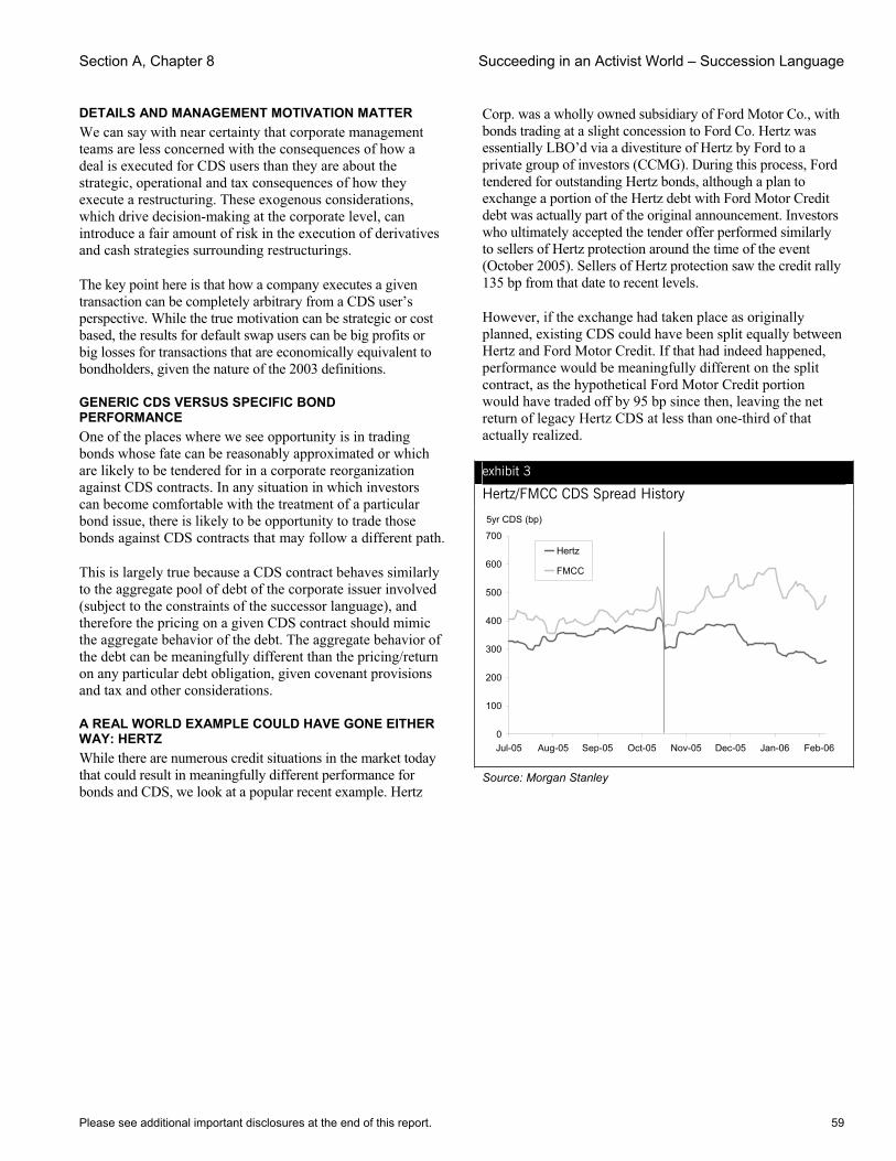
Section A, Chapter 8 Succeeding in an Activist World – Succession Language
Please see additional important disclosures at the end of this report. 59
DETAILS AND MANAGEMENT MOTIVATION MATTER We can say with near certainty that corporate management teams are less concerned with the consequences of how a deal is executed for CDS users than they are about the strategic, operational and tax consequences of how they execute a restructuring. These exogenous considerations, which drive decision-making at the corporate level, can introduce a fair amount of risk in the execution of derivatives and cash strategies surrounding restructurings.
The key point here is that how a company executes a given transaction can be completely arbitrary from a CDS user’s perspective. While the true motivation can be strategic or cost based, the results for default swap users can be big profits or big losses for transactions that are economically equivalent to bondholders, given the nature of the 2003 definitions.
GENERIC CDS VERSUS SPECIFIC BOND PERFORMANCE One of the places where we see opportunity is in trading bonds whose fate can be reasonably approximated or which are likely to be tendered for in a corporate reorganization against CDS contracts. In any situation in which investors can become comfortable with the treatment of a particular bond issue, there is likely to be opportunity to trade those bonds against CDS contracts that may follow a different path.
This is largely true because a CDS contract behaves similarly to the aggregate pool of debt of the corporate issuer involved (subject to the constraints of the successor language), and therefore the pricing on a given CDS contract should mimic the aggregate behavior of the debt. The aggregate behavior of the debt can be meaningfully different than the pricing/return on any particular debt obligation, given covenant provisions and tax and other considerations.
A REAL WORLD EXAMPLE COULD HAVE GONE EITHER WAY: HERTZ While there are numerous credit situations in the market today that could result in meaningfully different performance for bonds and CDS, we look at a popular recent example. Hertz
Corp. was a wholly owned subsidiary of Ford Motor Co., with bonds trading at a slight concession to Ford Co. Hertz was essentially LBO’d via a divestiture of Hertz by Ford to a private group of investors (CCMG). During this process, Ford tendered for outstanding Hertz bonds, although a plan to exchange a portion of the Hertz debt with Ford Motor Credit debt was actually part of the original announcement. Investors who ultimately accepted the tender offer performed similarly to sellers of Hertz protection around the time of the event (October 2005). Sellers of Hertz protection saw the credit rally 135 bp from that date to recent levels.
However, if the exchange had taken place as originally planned, existing CDS could have been split equally between Hertz and Ford Motor Credit. If that had indeed happened, performance would be meaningfully different on the split contract, as the hypothetical Ford Motor Credit portion would have traded off by 95 bp since then, leaving the net return of legacy Hertz CDS at less than one-third of that actually realized.
exhibit 3
Hertz/FMCC CDS Spread History
0
100
200
300
400
500
600
700
Jul-05 Aug-05 Sep-05 Oct-05 Nov-05 Dec-05 Jan-06 Feb-06
5yr CDS (bp)
Hertz
FMCC
Source: Morgan Stanley
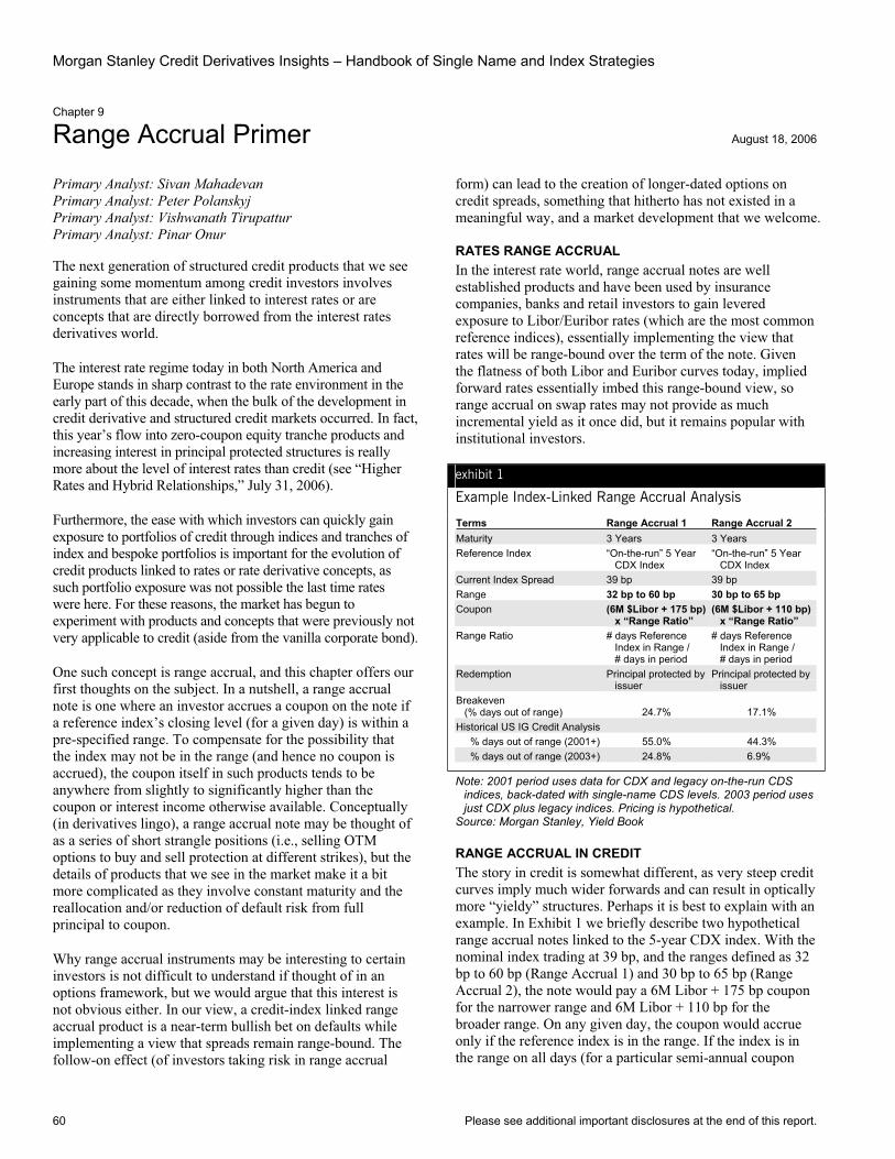
Morgan Stanley Credit Derivatives Insights – Handbook of Single Name and Index Strategies
60 Please see additional important disclosures at the end of this report.
Chapter 9
Range Accrual Primer August 18, 2006
Primary Analyst: Sivan Mahadevan Primary Analyst: Peter Polanskyj Primary Analyst: Vishwanath Tirupattur Primary Analyst: Pinar Onur
The next generation of structured credit products that we see gaining some momentum among credit investors involves instruments that are either linked to interest rates or are concepts that are directly borrowed from the interest rates derivatives world.
The interest rate regime today in both North America and Europe stands in sharp contrast to the rate environment in the early part of this decade, when the bulk of the development in credit derivative and structured credit markets occurred. In fact, this year’s flow into zero-coupon equity tranche products and increasing interest in principal protected structures is really more about the level of interest rates than credit (see “Higher Rates and Hybrid Relationships,” July 31, 2006).
Furthermore, the ease with which investors can quickly gain exposure to portfolios of credit through indices and tranches of index and bespoke portfolios is important for the evolution of credit products linked to rates or rate derivative concepts, as such portfolio exposure was not possible the last time rates were here. For these reasons, the market has begun to experiment with products and concepts that were previously not very applicable to credit (aside from the vanilla corporate bond).
One such concept is range accrual, and this chapter offers our first thoughts on the subject. In a nutshell, a range accrual note is one where an investor accrues a coupon on the note if a reference index’s closing level (for a given day) is within a pre-specified range. To compensate for the possibility that the index may not be in the range (and hence no coupon is accrued), the coupon itself in such products tends to be anywhere from slightly to significantly higher than the coupon or interest income otherwise available. Conceptually (in derivatives lingo), a range accrual note may be thought of as a series of short strangle positions (i.e., selling OTM options to buy and sell protection at different strikes), but the details of products that we see in the market make it a bit more complicated as they involve constant maturity and the reallocation and/or reduction of default risk from full principal to coupon.
Why range accrual instruments may be interesting to certain investors is not difficult to understand if thought of in an options framework, but we would argue that this interest is not obvious either. In our view, a credit-index linked range accrual product is a near-term bullish bet on defaults while implementing a view that spreads remain range-bound. The follow-on effect (of investors taking risk in range accrual
form) can lead to the creation of longer-dated options on credit spreads, something that hitherto has not existed in a meaningful way, and a market development that we welcome.
RATES RANGE ACCRUAL In the interest rate world, range accrual notes are well established products and have been used by insurance companies, banks and retail investors to gain levered exposure to Libor/Euribor rates (which are the most common reference indices), essentially implementing the view that rates will be range-bound over the term of the note. Given the flatness of both Libor and Euribor curves today, implied forward rates essentially imbed this range-bound view, so range accrual on swap rates may not provide as much incremental yield as it once did, but it remains popular with institutional investors.
exhibit 1
Example Index-Linked Range Accrual Analysis
Terms Range Accrual 1 Range Accrual 2 Maturity 3 Years 3 Years Reference Index “On-the-run” 5 Year
CDX Index “On-the-run” 5 Year
CDX Index Current Index Spread 39 bp 39 bp Range 32 bp to 60 bp 30 bp to 65 bp Coupon (6M $Libor + 175 bp)
x “Range Ratio” (6M $Libor + 110 bp)
x “Range Ratio” Range Ratio # days Reference
Index in Range / # days in period
# days Reference Index in Range / # days in period
Redemption Principal protected by issuer
Principal protected by issuer
Breakeven (% days out of range) 24.7% 17.1%
Historical US IG Credit Analysis % days out of range (2001+) 55.0% 44.3% % days out of range (2003+) 24.8% 6.9%
Note: 2001 period uses data for CDX and legacy on-the-run CDS indices, back-dated with single-name CDS levels. 2003 period uses just CDX plus legacy indices. Pricing is hypothetical.
Source: Morgan Stanley, Yield Book
RANGE ACCRUAL IN CREDIT The story in credit is somewhat different, as very steep credit curves imply much wider forwards and can result in optically more “yieldy” structures. Perhaps it is best to explain with an example. In Exhibit 1 we briefly describe two hypothetical range accrual notes linked to the 5-year CDX index. With the nominal index trading at 39 bp, and the ranges defined as 32 bp to 60 bp (Range Accrual 1) and 30 bp to 65 bp (Range Accrual 2), the note would pay a 6M Libor + 175 bp coupon for the narrower range and 6M Libor + 110 bp for the broader range. On any given day, the coupon would accrue only if the reference index is in the range. If the index is in the range on all days (for a particular semi-annual coupon
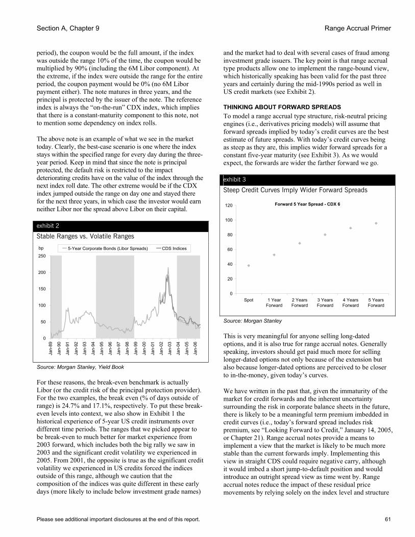
Section A, Chapter 9 Range Accrual Primer
Please see additional important disclosures at the end of this report. 61
period), the coupon would be the full amount, if the index was outside the range 10% of the time, the coupon would be multiplied by 90% (including the 6M Libor component). At the extreme, if the index were outside the range for the entire period, the coupon payment would be 0% (no 6M Libor payment either). The note matures in three years, and the principal is protected by the issuer of the note. The reference index is always the “on-the-run” CDX index, which implies that there is a constant-maturity component to this note, not to mention some dependency on index rolls.
The above note is an example of what we see in the market today. Clearly, the best-case scenario is one where the index stays within the specified range for every day during the three-year period. Keep in mind that since the note is principal protected, the default risk is restricted to the impact deteriorating credits have on the value of the index through the next index roll date. The other extreme would be if the CDX index jumped outside the range on day one and stayed there for the next three years, in which case the investor would earn neither Libor nor the spread above Libor on their capital.
exhibit 2
Stable Ranges vs. Volatile Ranges
bp
0
50
100
150
200
250
Jan-
89
Jan-
90
Jan-
91
Jan-
92
Jan-
93
Jan-
94
Jan-
95
Jan-
96
Jan-
97
Jan-
98
Jan-
99
Jan-
00
Jan-
01
Jan-
02
Jan-
03
Jan-
04
Jan-
05
Jan-
06
5-Year Corporate Bonds (Libor Spreads) CDS Indices
Source: Morgan Stanley, Yield Book
For these reasons, the break-even benchmark is actually Libor (or the credit risk of the principal protection provider). For the two examples, the break even (% of days outside of range) is 24.7% and 17.1%, respectively. To put these break-even levels into context, we also show in Exhibit 1 the historical experience of 5-year US credit instruments over different time periods. The ranges that we picked appear to be break-even to much better for market experience from 2003 forward, which includes both the big rally we saw in 2003 and the significant credit volatility we experienced in 2005. From 2001, the opposite is true as the significant credit volatility we experienced in US credits forced the indices outside of this range, although we caution that the composition of the indices was quite different in these early days (more likely to include below investment grade names)
and the market had to deal with several cases of fraud among investment grade issuers. The key point is that range accrual type products allow one to implement the range-bound view, which historically speaking has been valid for the past three years and certainly during the mid-1990s period as well in US credit markets (see Exhibit 2).
THINKING ABOUT FORWARD SPREADS To model a range accrual type structure, risk-neutral pricing engines (i.e., derivatives pricing models) will assume that forward spreads implied by today’s credit curves are the best estimate of future spreads. With today’s credit curves being as steep as they are, this implies wider forward spreads for a constant five-year maturity (see Exhibit 3). As we would expect, the forwards are wider the farther forward we go.
exhibit 3
Steep Credit Curves Imply Wider Forward Spreads
Forward 5 Year Spread - CDX 6
0
20
40
60
80
100
120
Spot 1 YearForward
2 YearsForward
3 YearsForward
4 YearsForward
5 YearsForward
Source: Morgan Stanley
This is very meaningful for anyone selling long-dated options, and it is also true for range accrual notes. Generally speaking, investors should get paid much more for selling longer-dated options not only because of the extension but also because longer-dated options are perceived to be closer to in-the-money, given today’s curves.
We have written in the past that, given the immaturity of the market for credit forwards and the inherent uncertainty surrounding the risk in corporate balance sheets in the future, there is likely to be a meaningful term premium imbedded in credit curves (i.e., today’s forward spread includes risk premium, see “Looking Forward to Credit,” January 14, 2005, or Chapter 21). Range accrual notes provide a means to implement a view that the market is likely to be much more stable than the current forwards imply. Implementing this view in straight CDS could require negative carry, although it would imbed a short jump-to-default position and would introduce an outright spread view as time went by. Range accrual notes reduce the impact of these residual price movements by relying solely on the index level and structure

Morgan Stanley Credit Derivatives Insights – Handbook of Single Name and Index Strategies
62 Please see additional important disclosures at the end of this report.
to determine the coupon cashflows while the principal remains unexposed to defaults or spread moves.
Another point worth raising is that investors are not simply selling volatility in these structures. Because of steep credit curves, the series of options actually being sold in these structures vary in their moneyness. Clearly, near term options are out of the money but because of steep credit curves, the longer-dated options appear in the money (at least based on forwards). Therefore, the impact of changing volatility on these notes is not as obvious as one would think. Volatility in the short term is likely a negative but increased volatility in the long term can actually be beneficial as it could result in spreads staying within the range while market expectations may be the opposite. So the net volatility position is more muted than that of just purely selling a strangle.
THE INDEX ROLL – CHANGING CREDIT PROFILE The index roll is much harder to model in a derivative framework, but what a range accrual buyer signs up for is exposure to a new index every roll period, based on the market conventions for rolling . Current market practice is as follows. Every six months, indices are rebalanced based on specific guidelines including S&P and Moody’s ratings, recent corporate actions, and outstanding debt or liquidity. In particular, based on each CDX member firm’s judgment, entities rated below investment grade by either S&P or Moody’s should not be included in the new index. We caution that these guidelines and market practices could change.
Why is rolling better or worse than sticking to the same index for the life of the trade? Rolling clearly improves liquidity, although there is “uncertainty” associated with which credits an investor is exposed to. However, getting exposure to a new index every six months that promises to be investment grade changes the risk profile quite substantially compared to a constant index. Based on ratings history, investment grade credits tend to have net negative ratings migration patterns – see Exhibit 4, where 18% of Baa credits have experienced a downgrade to high yield (including defaults) over all three-year periods since 1983, according to Moody’s.
exhibit 4
Three-Year Transition
Aaa Aa A Baa Below IG WRAaa 85.4% 13.7% 0.2% 0.0% 0.0% 0.7%Aa 11.6% 79.3% 3.5% 0.1% 0.0% 5.4%A 0.4% 7.4% 78.0% 7.1% 2.0% 5.1%Baa 0.0% 0.7% 19.5% 50.8% 17.9% 11.2%
Note: 3-year ratings transitions are based on annual Moody’s cohorts from 1983 forward.
Source: Morgan Stanley, Moody’s
From a long credit perspective, exposure to credits that are investment grade at the beginning of a six-month period is perhaps a better macro bet on credit quality than one where
credits are allowed to deteriorate as we see in the Moody’s data. Also, the default risk that one is exposed to is clearly jump-to-default fallen-angel type risk (IG to default in six months), which we would argue is markedly less likely than an investment grade name moving to default over several years.
THE INDEX ROLL – RANGE MECHANICS In terms of mechanics, the range in some range accrual notes resets at every index roll to reflect any spread differential between the now off-the-run index and the new on-the-run index. The idea is to avoid exposing investors to changes in the index spread related solely to the change in constituent names. While there is no market standard, typical structures have a mechanism to calculate a maturity equivalent spread for both the new and the old index and would then adjust the range so the new range is roughly equivalent to the old range given the absolute price level. For example, if the old index maturity equivalent spread is 50 bp with an old range of 40 to 60 bp (+/-20%), and the new index is 40 bp, the range would be reset to 32 to 48 bp (also +/- 20%).
PRINCIPAL PROTECTION Another feature we see in the market is that the seller of protection on an index with range accrual is not really selling protection because the principal is not exposed to defaults. One can think of this as principal protection (where the principal protection is offered by a counterparty like a broker-dealer, but could also be provided by another entity), but the default exposure in the index does not disappear.
The default risk is reflected through adjustments to the range based on the price impact of a default on the index. The result is to treat extreme widenings in spreads and actual defaults in the same way. Again, we will use an example to illustrate. Let’s assume the on-the-run index trades at 40 bp and examine the price impact of two scenarios. First, a credit trades down 55 points in price but does not default and, second, a credit defaults with a 45% recovery.
In the first case, the price impact of the widening would be worth about 10 bp running on the index (55% loss / PV01 / 125 names) with that widening reflected when the index rolled (as we illustrate above) and the name likely removed from the new index. The second case (default) is actually treated the same way in a range accrual note by reflecting the value of the default on the index in the roll calculation, even though in a simple index transaction, the seller of protection would have to pay out to settle the default.
From a practical perspective, the impact of a deteriorating credit (including a default) is to effectively narrow the range of the range accrual note upon an index roll, which at the extreme (after many defaults), could be small enough to result in a low likelihood of receiving coupon income. So the coupon in this type of range accrual note is very sensitive to defaults, while the principal is protected from them.

Section A, Chapter 9 Range Accrual Primer
Please see additional important disclosures at the end of this report. 63
CONCLUSIONWe are very much in the early days of applying concepts like range accrual to the credit markets. At one level, we are happy to see it happen as it gives investors a convenient way to implement (with leverage) the range-bound spread view that gets espoused by investors, traders and even strategists frequently. At another level, range accrual will help a long-dated options market develop as well, which is something the market needs if option-strategies are to become a dependable tool in the credit portfolio manager’s toolkit.
We stop short of making investment recommendations on range accrual at this point, and instead encourage investors who are not afraid to test innovation to take the first steps in this direction, especially if they have the range-bound view. The mechanics that we have described in this chapter are somewhat specialized, but the concept is not, which is what investors should probably focus on first.
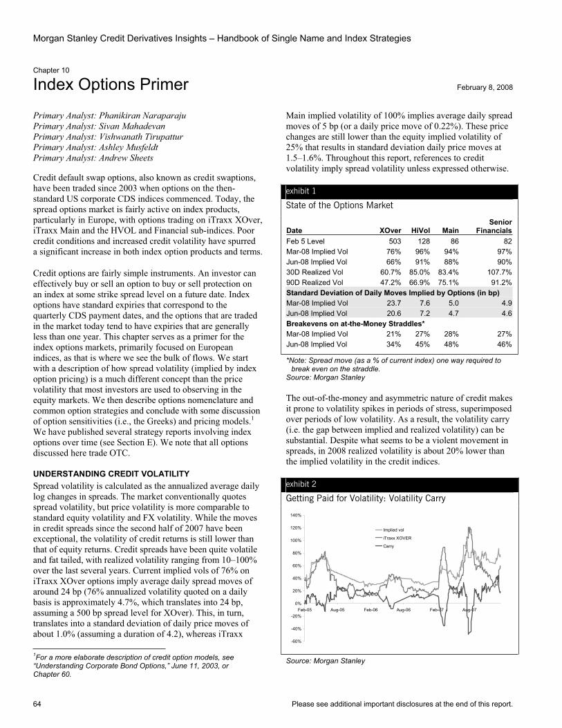
Morgan Stanley Credit Derivatives Insights – Handbook of Single Name and Index Strategies
64 Please see additional important disclosures at the end of this report.
Chapter 10
Index Options Primer February 8, 2008
Primary Analyst: Phanikiran Naraparaju Primary Analyst: Sivan Mahadevan Primary Analyst: Vishwanath Tirupattur Primary Analyst: Ashley Musfeldt Primary Analyst: Andrew Sheets
Credit default swap options, also known as credit swaptions, have been traded since 2003 when options on the then-standard US corporate CDS indices commenced. Today, the spread options market is fairly active on index products, particularly in Europe, with options trading on iTraxx XOver, iTraxx Main and the HVOL and Financial sub-indices. Poor credit conditions and increased credit volatility have spurred a significant increase in both index option products and terms.
Credit options are fairly simple instruments. An investor can effectively buy or sell an option to buy or sell protection on an index at some strike spread level on a future date. Index options have standard expiries that correspond to the quarterly CDS payment dates, and the options that are traded in the market today tend to have expiries that are generally less than one year. This chapter serves as a primer for the index options markets, primarily focused on European indices, as that is where we see the bulk of flows. We start with a description of how spread volatility (implied by index option pricing) is a much different concept than the price volatility that most investors are used to observing in the equity markets. We then describe options nomenclature and common option strategies and conclude with some discussion of option sensitivities (i.e., the Greeks) and pricing models.1We have published several strategy reports involving index options over time (see Section E). We note that all options discussed here trade OTC.
UNDERSTANDING CREDIT VOLATILITY Spread volatility is calculated as the annualized average daily log changes in spreads. The market conventionally quotes spread volatility, but price volatility is more comparable to standard equity volatility and FX volatility. While the moves in credit spreads since the second half of 2007 have been exceptional, the volatility of credit returns is still lower than that of equity returns. Credit spreads have been quite volatile and fat tailed, with realized volatility ranging from 10–100% over the last several years. Current implied vols of 76% on iTraxx XOver options imply average daily spread moves of around 24 bp (76% annualized volatility quoted on a daily basis is approximately 4.7%, which translates into 24 bp, assuming a 500 bp spread level for XOver). This, in turn, translates into a standard deviation of daily price moves of about 1.0% (assuming a duration of 4.2), whereas iTraxx 1For a more elaborate description of credit option models, see “Understanding Corporate Bond Options,” June 11, 2003, or Chapter 60.
Main implied volatility of 100% implies average daily spread moves of 5 bp (or a daily price move of 0.22%). These price changes are still lower than the equity implied volatility of 25% that results in standard deviation daily price moves at 1.5–1.6%. Throughout this report, references to credit volatility imply spread volatility unless expressed otherwise.
exhibit 1
State of the Options Market
Date XOver HiVol MainSenior
FinancialsFeb 5 Level 503 128 86 82Mar-08 Implied Vol 76% 96% 94% 97%Jun-08 Implied Vol 66% 91% 88% 90%30D Realized Vol 60.7% 85.0% 83.4% 107.7%90D Realized Vol 47.2% 66.9% 75.1% 91.2%Standard Deviation of Daily Moves Implied by Options (in bp) Mar-08 Implied Vol 23.7 7.6 5.0 4.9Jun-08 Implied Vol 20.6 7.2 4.7 4.6Breakevens on at-the-Money Straddles* Mar-08 Implied Vol 21% 27% 28% 27%Jun-08 Implied Vol 34% 45% 48% 46%
*Note: Spread move (as a % of current index) one way required to break even on the straddle.
Source: Morgan Stanley
The out-of-the-money and asymmetric nature of credit makes it prone to volatility spikes in periods of stress, superimposed over periods of low volatility. As a result, the volatility carry (i.e. the gap between implied and realized volatility) can be substantial. Despite what seems to be a violent movement in spreads, in 2008 realized volatility is about 20% lower than the implied volatility in the credit indices.
exhibit 2
Getting Paid for Volatility: Volatility Carry
-60%
-40%
-20%
0%
20%
40%
60%
80%
100%
120%
140%
Feb-05 Aug-05 Feb-06 Aug-06 Feb-07 Aug-07
Implied vol
iTraxx XOVER
Carry
Source: Morgan Stanley
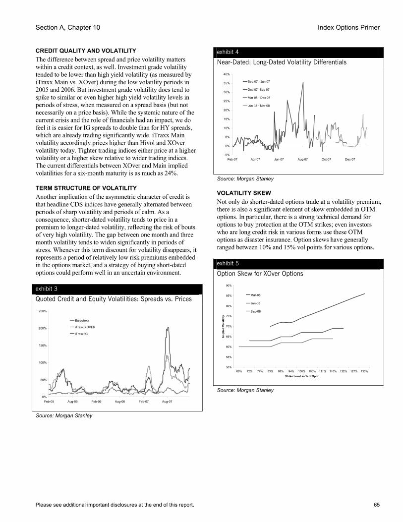
Section A, Chapter 10 Index Options Primer
Please see additional important disclosures at the end of this report. 65
CREDIT QUALITY AND VOLATILITY The difference between spread and price volatility matters within a credit context, as well. Investment grade volatility tended to be lower than high yield volatility (as measured by iTraxx Main vs. XOver) during the low volatility periods in 2005 and 2006. But investment grade volatility does tend to spike to similar or even higher high yield volatility levels in periods of stress, when measured on a spread basis (but not necessarily on a price basis). While the systemic nature of the current crisis and the role of financials had an impact, we do feel it is easier for IG spreads to double than for HY spreads, which are already trading significantly wide. iTraxx Main volatility accordingly prices higher than Hivol and XOver volatility today. Tighter trading indices either price at a higher volatility or a higher skew relative to wider trading indices. The current differentials between XOver and Main implied volatilities for a six-month maturity is as much as 24%.
TERM STRUCTURE OF VOLATILITY Another implication of the asymmetric character of credit is that headline CDS indices have generally alternated between periods of sharp volatility and periods of calm. As a consequence, shorter-dated volatility tends to price in a premium to longer-dated volatility, reflecting the risk of bouts of very high volatility. The gap between one month and three month volatility tends to widen significantly in periods of stress. Whenever this term discount for volatility disappears, it represents a period of relatively low risk premiums embedded in the options market, and a strategy of buying short-dated options could perform well in an uncertain environment.
exhibit 3
Quoted Credit and Equity Volatilities: Spreads vs. Prices
0%
50%
100%
150%
200%
250%
Feb-05 Aug-05 Feb-06 Aug-06 Feb-07 Aug-07
Eurostoxx
iTraxx XOVER
iTraxx IG
Source: Morgan Stanley
exhibit 4
Near-Dated: Long-Dated Volatility Differentials
-5%
0%
5%
10%
15%
20%
25%
30%
35%
40%
Feb-07 Apr-07 Jun-07 Aug-07 Oct-07 Dec-07
Sep 07 - Jun 07
Dec 07 -Sep 07
Mar 08 - Dec 07
Jun 08 - Mar 08
Source: Morgan Stanley
VOLATILITY SKEW Not only do shorter-dated options trade at a volatility premium, there is also a significant element of skew embedded in OTM options. In particular, there is a strong technical demand for options to buy protection at the OTM strikes; even investors who are long credit risk in various forms use these OTM options as disaster insurance. Option skews have generally ranged between 10% and 15% vol points for various options.
exhibit 5
Option Skew for XOver Options
50%
55%
60%
65%
70%
75%
80%
85%
90%
66% 72% 77% 83% 88% 94% 100% 105% 111% 116% 122% 127% 133%
Strike Level as % of Spot
Impl
ied
Vola
tility
Mar-08
Jun-08
Sep-08
Source: Morgan Stanley
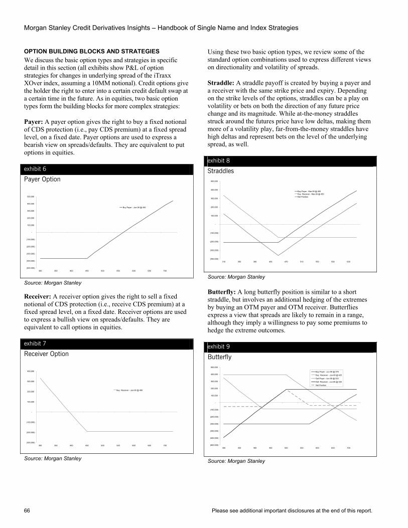
Morgan Stanley Credit Derivatives Insights – Handbook of Single Name and Index Strategies
66 Please see additional important disclosures at the end of this report.
OPTION BUILDING BLOCKS AND STRATEGIES We discuss the basic option types and strategies in specific detail in this section (all exhibits show P&L of option strategies for changes in underlying spread of the iTraxx XOver index, assuming a 10MM notional). Credit options give the holder the right to enter into a certain credit default swap at a certain time in the future. As in equities, two basic option types form the building blocks for more complex strategies:
Payer: A payer option gives the right to buy a fixed notional of CDS protection (i.e., pay CDS premium) at a fixed spread level, on a fixed date. Payer options are used to express a bearish view on spreads/defaults. They are equivalent to put options in equities.
exhibit 6
Payer Option
(500,000)
(400,000)
(300,000)
(200,000)
(100,000)
-
100,000
200,000
300,000
400,000
500,000
300 350 400 450 500 550 600 650 700
Buy Payer - Jun-08 @ 450
Source: Morgan Stanley
Receiver: A receiver option gives the right to sell a fixed notional of CDS protection (i.e., receive CDS premium) at a fixed spread level, on a fixed date. Receiver options are used to express a bullish view on spreads/defaults. They are equivalent to call options in equities.
exhibit 7
Receiver Option
(300,000)
(200,000)
(100,000)
-
100,000
200,000
300,000
400,000
300 350 400 450 500 550 600 650 700
Buy Receiver - Jun-08 @ 450
Source: Morgan Stanley
Using these two basic option types, we review some of the standard option combinations used to express different views on directionality and volatility of spreads.
Straddle: A straddle payoff is created by buying a payer and a receiver with the same strike price and expiry. Depending on the strike levels of the options, straddles can be a play on volatility or bets on both the direction of any future price change and its magnitude. While at-the-money straddles struck around the futures price have low deltas, making them more of a volatility play, far-from-the-money straddles have high deltas and represent bets on the level of the underlying spread, as well.
exhibit 8
Straddles
(400,000)
(300,000)
(200,000)
(100,000)
-
100,000
200,000
300,000
400,000
500,000
310 350 390 430 470 510 550 590 630
Buy Payer - Mar-08 @ 450Buy Receiver - Mar-08 @ 450Net Position
Source: Morgan Stanley
Butterfly: A long butterfly position is similar to a short straddle, but involves an additional hedging of the extremes by buying an OTM payer and OTM receiver. Butterflies express a view that spreads are likely to remain in a range, although they imply a willingness to pay some premiums to hedge the extreme outcomes.
exhibit 9
Butterfly
(600,000)
(500,000)
(400,000)
(300,000)
(200,000)
(100,000)
-
100,000
200,000
300,000
400,000
500,000
300 350 400 450 500 550 600 650 700
Buy Payer - Jun-08 @ 575
Buy Receiver - Jun-08 @ 425
Sell Payer - Jun-08 @ 500
Sell Receiver - Jun-08 @ 500
Net Position
Source: Morgan Stanley
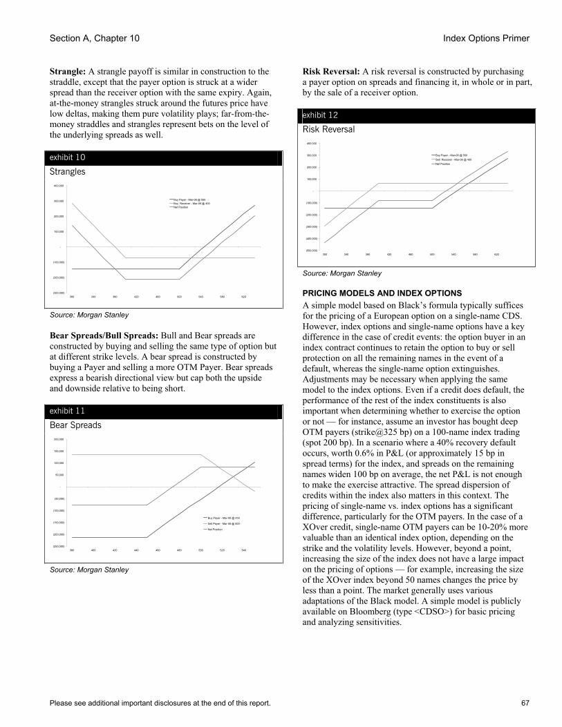
Section A, Chapter 10 Index Options Primer
Please see additional important disclosures at the end of this report. 67
Strangle: A strangle payoff is similar in construction to the straddle, except that the payer option is struck at a wider spread than the receiver option with the same expiry. Again, at-the-money strangles struck around the futures price have low deltas, making them pure volatility plays; far-from-the-money straddles and strangles represent bets on the level of the underlying spreads as well.
exhibit 10
Strangles
(300,000)
(200,000)
(100,000)
-
100,000
200,000
300,000
400,000
300 340 380 420 460 500 540 580 620
Buy Payer - Mar-08 @ 500Buy Receiver - Mar-08 @ 400Net Position
Source: Morgan Stanley
Bear Spreads/Bull Spreads: Bull and Bear spreads are constructed by buying and selling the same type of option but at different strike levels. A bear spread is constructed by buying a Payer and selling a more OTM Payer. Bear spreads express a bearish directional view but cap both the upside and downside relative to being short.
exhibit 11
Bear Spreads
(250,000)
(200,000)
(150,000)
(100,000)
(50,000)
-
50,000
100,000
150,000
200,000
380 400 420 440 460 480 500 520 540
Buy Payer - Mar-08 @ 450
Sell Payer - Mar-08 @ 500
Net Position
Source: Morgan Stanley
Risk Reversal: A risk reversal is constructed by purchasing a payer option on spreads and financing it, in whole or in part, by the sale of a receiver option.
exhibit 12
Risk Reversal
(500,000)
(400,000)
(300,000)
(200,000)
(100,000)
-
100,000
200,000
300,000
400,000
300 340 380 420 460 500 540 580 620
Buy Payer - Mar-08 @ 500Sell Receiver - Mar-08 @ 400Net Position
Source: Morgan Stanley
PRICING MODELS AND INDEX OPTIONS A simple model based on Black’s formula typically suffices for the pricing of a European option on a single-name CDS. However, index options and single-name options have a key difference in the case of credit events: the option buyer in an index contract continues to retain the option to buy or sell protection on all the remaining names in the event of a default, whereas the single-name option extinguishes. Adjustments may be necessary when applying the same model to the index options. Even if a credit does default, the performance of the rest of the index constituents is also important when determining whether to exercise the option or not — for instance, assume an investor has bought deep OTM payers (strike@325 bp) on a 100-name index trading (spot 200 bp). In a scenario where a 40% recovery default occurs, worth 0.6% in P&L (or approximately 15 bp in spread terms) for the index, and spreads on the remaining names widen 100 bp on average, the net P&L is not enough to make the exercise attractive. The spread dispersion of credits within the index also matters in this context. The pricing of single-name vs. index options has a significant difference, particularly for the OTM payers. In the case of a XOver credit, single-name OTM payers can be 10-20% more valuable than an identical index option, depending on the strike and the volatility levels. However, beyond a point, increasing the size of the index does not have a large impact on the pricing of options — for example, increasing the size of the XOver index beyond 50 names changes the price by less than a point. The market generally uses various adaptations of the Black model. A simple model is publicly available on Bloomberg (type <CDSO>) for basic pricing and analyzing sensitivities.
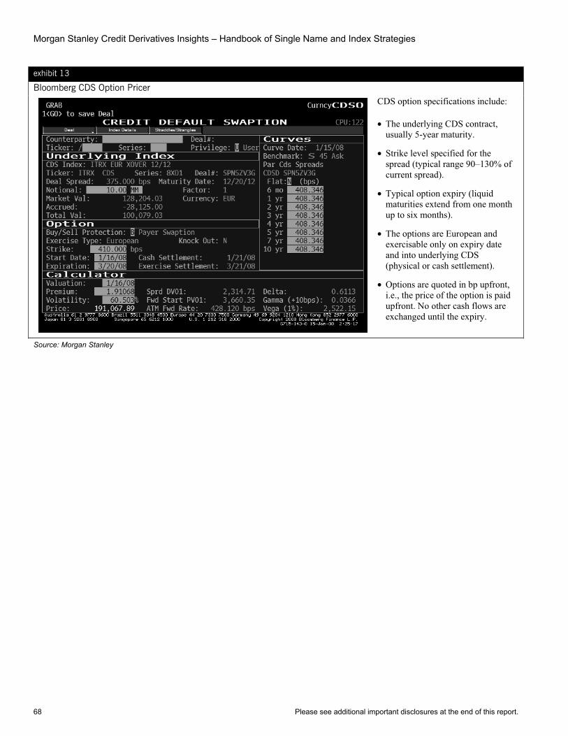
Morgan Stanley Credit Derivatives Insights – Handbook of Single Name and Index Strategies
68 Please see additional important disclosures at the end of this report.
exhibit 13
Bloomberg CDS Option Pricer CDS option specifications include:
• The underlying CDS contract, usually 5-year maturity.
• Strike level specified for the spread (typical range 90–130% of current spread).
• Typical option expiry (liquid maturities extend from one month up to six months).
• The options are European and exercisable only on expiry date and into underlying CDS (physical or cash settlement).
• Options are quoted in bp upfront, i.e., the price of the option is paid upfront. No other cash flows are exchanged until the expiry.
Source: Morgan Stanley
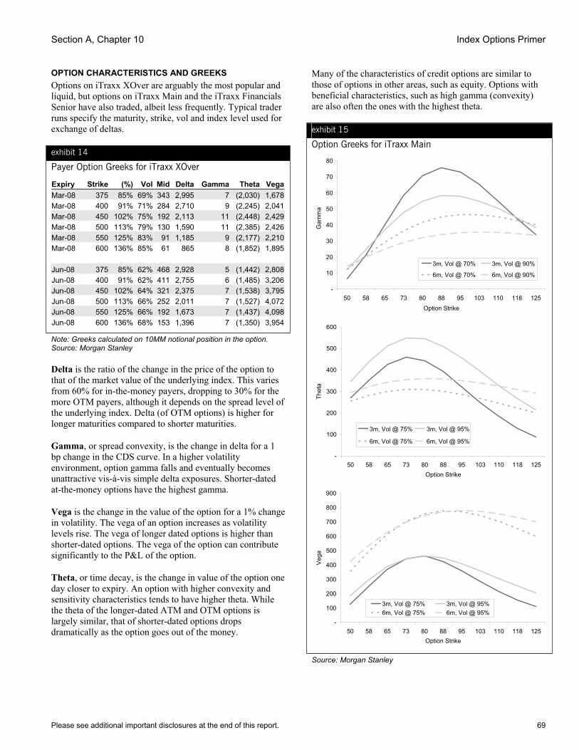
Section A, Chapter 10 Index Options Primer
Please see additional important disclosures at the end of this report. 69
OPTION CHARACTERISTICS AND GREEKS Options on iTraxx XOver are arguably the most popular and liquid, but options on iTraxx Main and the iTraxx Financials Senior have also traded, albeit less frequently. Typical trader runs specify the maturity, strike, vol and index level used for exchange of deltas.
exhibit 14
Payer Option Greeks for iTraxx XOver
Expiry Strike (%) Vol Mid Delta Gamma Theta VegaMar-08 375 85% 69% 343 2,995 7 (2,030) 1,678Mar-08 400 91% 71% 284 2,710 9 (2,245) 2,041Mar-08 450 102% 75% 192 2,113 11 (2,448) 2,429Mar-08 500 113% 79% 130 1,590 11 (2,385) 2,426Mar-08 550 125% 83% 91 1,185 9 (2,177) 2,210Mar-08 600 136% 85% 61 865 8 (1,852) 1,895 Jun-08 375 85% 62% 468 2,928 5 (1,442) 2,808Jun-08 400 91% 62% 411 2,755 6 (1,485) 3,206Jun-08 450 102% 64% 321 2,375 7 (1,538) 3,795Jun-08 500 113% 66% 252 2,011 7 (1,527) 4,072Jun-08 550 125% 66% 192 1,673 7 (1,437) 4,098Jun-08 600 136% 68% 153 1,396 7 (1,350) 3,954
Note: Greeks calculated on 10MM notional position in the option. Source: Morgan Stanley
Delta is the ratio of the change in the price of the option to that of the market value of the underlying index. This varies from 60% for in-the-money payers, dropping to 30% for the more OTM payers, although it depends on the spread level of the underlying index. Delta (of OTM options) is higher for longer maturities compared to shorter maturities.
Gamma, or spread convexity, is the change in delta for a 1 bp change in the CDS curve. In a higher volatility environment, option gamma falls and eventually becomes unattractive vis-à-vis simple delta exposures. Shorter-dated at-the-money options have the highest gamma.
Vega is the change in the value of the option for a 1% change in volatility. The vega of an option increases as volatility levels rise. The vega of longer dated options is higher than shorter-dated options. The vega of the option can contribute significantly to the P&L of the option.
Theta, or time decay, is the change in value of the option one day closer to expiry. An option with higher convexity and sensitivity characteristics tends to have higher theta. While the theta of the longer-dated ATM and OTM options is largely similar, that of shorter-dated options drops dramatically as the option goes out of the money.
Many of the characteristics of credit options are similar to those of options in other areas, such as equity. Options with beneficial characteristics, such as high gamma (convexity) are also often the ones with the highest theta.
exhibit 15
Option Greeks for iTraxx Main
-
10
20
30
40
50
60
70
80
50 58 65 73 80 88 95 103 110 118 125Option Strike
Gam
ma
3m, Vol @ 70% 3m, Vol @ 90%
6m, Vol @ 70% 6m, Vol @ 90%
-
100
200
300
400
500
600
50 58 65 73 80 88 95 103 110 118 125Option Strike
Thet
a
3m, Vol @ 75% 3m, Vol @ 95%
6m, Vol @ 75% 6m, Vol @ 95%
-
100
200
300
400
500
600
700
800
900
50 58 65 73 80 88 95 103 110 118 125Option Strike
Veg
a
3m, Vol @ 75% 3m, Vol @ 95%6m, Vol @ 75% 6m, Vol @ 95%
Source: Morgan Stanley

Morgan Stanley Credit Derivatives Insights – Handbook of Single Name and Index Strategies
70 Please see additional important disclosures at the end of this report.
Chapter 11
Muni Mania February 1, 2008
Primary Analyst: Ashley Musfeldt Primary Analyst: Sivan Mahadevan Primary Analyst: Vishwanath Tirupattur Primary Analyst: Andrew Sheets Primary Analyst: Phanikiran Naraparaju
One of the strongest themes that emerged in the latter half of 2007 was the significant pickup in systemic risk across the global financial system. The impact of this systemic risk had and continues to have huge negative implications on risky credit assets, but it has also led to growth and participation in new credit market instruments. In Europe there has been an explosion in the usage of sovereign CDS as a tool to hedge systemic risk, position for sovereign stress and also capture the unprecedented wide spreads on sovereign entities in leveraged and structured products. CDS on European sovereign names now trade in the 10 to 40 bp range.
These same systemic market themes have played a role in the explosive recent growth of credit default swaps on US municipal issuers. US housing stress, state-specific economic conditions and the monoline debacle have clearly played a role as well. Up until last summer the over $2.2 trillion US municipal market was, despite its size, a quiet market. States, counties, cities, school districts and other entities that could borrow at tax-exempt rates would bring their issue to market, where much of it would be sold to individual investors and nearly all of it was purchased with the expectation that it would be held to maturity.
exhibit 1
Current Indicative Levels for Muni CDS (As of January 31, 2008)
Issuer State Moody’s S&P 10YR CDSCalifornia CA A1 A+ 58/65New York, NY NY Aa3 AA 46/53Florida FL Aa1 AAA 44/52Michigan MI Aa3 AA- 43/51Ohio OH Aa1 AA+ 37/43New Jersey NJ Aa3 AA 36/42New York State NY Aa3 AA 35/41Illinois IL Aa3 AA 25/31Massachusetts MA Aa2 AA 22/28Texas TX Aa1 AA 21/27
Source: Morgan Stanley Research
When the first signs of the impending housing issues began to surface in February, market participants began to connect the dots. If foreclosures and bankruptcies really were on the rise, this could lead to a dramatic reduction in tax revenues. The virtually non-existent municipal CDS market suddenly seemed like a good place to speculate on the state of the US
housing market. We estimate that the volume of muni CDS trading has gone from several hundred million total in the 5 years prior to July 2007 to over $50 billion in the 6 months since then.
exhibit 2
Historical Spreads on Muni CDS
0
10
20
30
40
50
60
70
Jun-07 Jul-07 Sep-07 Oct-07 Dec-07 Jan-08
California New York State New Jersey Florida
Source: Morgan Stanley Research
Further compounding the trouble in the municipal market is the uncertain monoline situation. Though the monolines have run into trouble insuring ABS CDO paper, their original business plan was insuring the municipal bond market (indeed, MBIA initially stood for Municipal Bond Insurance Association). With the monolines’ future ability to pay out claims or even write new business in question, the municipal market was threatened with the notion that hundreds of billions of dollars of insurance wraps are deemed much less valuable than just a few months ago. While most of the G.O. debt that is referenced in the CDS market isn’t wrapped by monolines, the deteriorating credit quality of the monolines was causing more uncertainty in an already shaken market. Many new issues were put on hold, while the market waited for some resolution.
Finally, many investors realized that municipalities’ expenses tend to be rather fixed, while tax revenues can vary widely year to year based on economic conditions and that municipalities can be reluctant to raise taxes prematurely.
Meanwhile, as the new issue market was coming under pressure, the CDS volumes were increasing. Buyers of protection further pushed the credit spreads wider as more non-traditional funds entered the market from the short side. Exhibit 2 shows the CDS spreads, historically in the single digits, widen to 40, 50, 60 bps and Exhibit 1 shows indicative levels on 10 liquid names as of January 31.
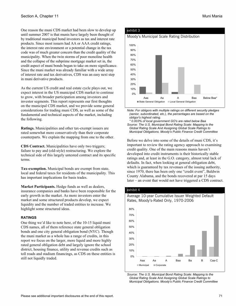
Section A, Chapter 11 Muni Mania
Please see additional important disclosures at the end of this report. 71
One reason the muni CDS market had been slow to develop up until summer 2007 is that munis have largely been thought of by traditional municipal bond investors as tax and interest rate products. Since most issuers had AA or AAA credit ratings, the interest rate environment or a potential change in the tax code was of much greater concern than the credit quality of the municipality. When the twin storms of poor monoline health and the collapse of the subprime mortgage market set in, the credit aspect of muni bonds began to take on more significance. Since the muni market was already familiar with a wide array of interest rate and tax derivatives, CDS was an easy next step in muni derivative products.
As the current US credit and real estate cycle plays out, we expect interest in the US municipal CDS market to continue to grow, with broader participation among investors and investor segments. This report represents our first thoughts on the municipal CDS market, and we provide some general considerations for trading muni CDS, as well as some of the fundamental and technical aspects of the market, including the following.
Ratings. Municipalities and other tax-exempt issuers are rated somewhat more conservatively than their corporate counterparts. We explain the mapping from one to the other.
CDS Contract. Municipalities have only two triggers; failure to pay and (old-style) restructuring. We explore the technical side of this largely untested contract and its specific terms.
Tax-exemption. Municipal bonds are exempt from state, local and federal taxes for residents of the municipality. This has important implications for basis trades.
Market Participants. Hedge funds as well as dealers, insurance companies and banks have been responsible for the early growth in the market. As more investors enter the market and some structured products develop, we expect liquidity and the number of traded entities to increase. We highlight some structured ideas.
RATINGS One thing we’d like to note here, of the 10-15 liquid muni CDS names, all of them reference state general obligation bonds and one city general obligation bond (NYC). Though the muni market as a whole has a range of credits, in this report we focus on the larger, more liquid and more highly rated general obligation debt and largely ignore the school district, housing finance, utility and revenue credits such as toll roads and stadium financings, as CDS on these entities is still not liquidly traded.
exhibit 3
Moody’s Municipal Scale Rating Distribution
0%
10%
20%
30%
40%
50%
60%
70%
80%
90%
100%
Aaa Aa A Baa Below Baa*State General Obligation Local General Obligation
Note: For obligors with multiple ratings on different security pledges (senior, subordinated, etc.), the percentages are based on the obligor's highest rating. * 0.003% of local government GO's are rated below Baa
Source: The U.S. Municipal Bond Rating Scale: Mapping to the Global Rating Scale And Assigning Global Scale Ratings to Municipal Obligations. Moody's Public Finance Credit Committee
Before we delve into some of the details of muni CDS, it’s important to review the rating agency approach to examining credit quality. One of the main reasons munis haven’t developed into credit instruments is their historically stable ratings and, at least in the G.O. category, almost total lack of defaults. In fact, when looking at general obligation debt, which is guaranteed by tax revenues of the issuing authority, since 1970, there has been only one “credit event”, Baldwin County Alabama, and the bonds recovered at par 15 days later – an event that would not have triggered a CDS contract.
exhibit 4
Average 10-year Cumulative Issuer Weighted Default Rates, Moody’s-Rated Only, 1970-2006
0%
10%
20%
30%
40%
50%
60%
70%
80%
Aaa Aa A Baa Ba B Caa-CMunicipal Corporate
Source: The U.S. Municipal Bond Rating Scale: Mapping to the Global Rating Scale And Assigning Global Scale Ratings to Municipal Obligations. Moody's Public Finance Credit Committee
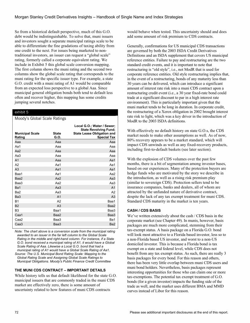
Morgan Stanley Credit Derivatives Insights – Handbook of Single Name and Index Strategies
72 Please see additional important disclosures at the end of this report.
So from a historical default perspective, much of this G.O. debt would be indistinguishable. To solve that, muni issuers and investors sought a separate municipal ratings scale to be able to differentiate the fine gradations of taxing ability from one credit to the next. For issues being marketed to non-traditional investors, an issuer can request a “global scale” rating, formerly called a corporate equivalent rating. We include in Exhibit 5 this global scale conversion mapping. The first column shows the muni rating and the second two columns show the global scale rating that corresponds to the muni rating for the specific issuer type. For example, a state G.O. credit with a muni rating of A1 would be comparable from an expected loss perspective to a global Aaa. Since municipal general obligation bonds both tend to default less often and recover higher, this mapping has some credits jumping several notches.
exhibit 5
Moody’s Global Scale Ratings
Municipal Scale Rating
StateG.O.
Local G.O.; Water / Sewer; State Revolving Fund;
State Lease Obligation and Special Tax
Aaa Aaa AaaAa1 Aaa AaaAa2 Aaa AaaAa3 Aaa AaaA1 Aaa Aa1A2 Aa1 Aa1A3 Aa1 Aa1Baa1 Aa1 Aa2Baa2 Aa2 Aa3Baa3 Aa2 Aa3Ba1 Aa3 A1Ba2 Aa3 A2Ba3 A1 A3B1 A2 Baa1B2 A3 Baa2B3 Baa1 Baa3Caa1 Baa2 Baa3Caa2 Baa3 Ba1Caa3 Baa3 Ba2
Note: The chart above is a conversion scale from the municipal rating awarded to an issuer in the far left column to the Global Scale Rating in the middle and right-hand column. For instance, if a State G.O. bond received a municipal rating of A1, it would have a Global Scale Rating of Aaa. Likewise a Local G.O. bond that had a municipal rating of A1 would have a Global Scale Rating of Aa1.
Source: The U.S. Municipal Bond Rating Scale: Mapping to the Global Rating Scale and Assigning Global Scale Ratings to Municipal Obligations. Moody's Public Finance Credit Committee
THE MUNI CDS CONTRACT – IMPORTANT DETAILS While history tells us that default likelihood for the state G.O. municipal issuers that are commonly traded in the muni CDS market are effectively zero, there is some amount of uncertainty related to how features of muni CDS contracts
would behave when tested. This uncertainty should and does add some amount of risk premium to CDS contracts.
Generally, confirmations for US municipal CDS transactions are governed by both the 2003 ISDA Credit Derivatives Definitions and an ISDA supplement that covers US municipal reference entities. Failure to pay and restructuring are the two standard credit events, and it is important to note that restructuring is “old style”, i.e., not ModR that is used for corporate reference entities. Old style restructuring implies that, in the event of a restructuring, bonds of any maturity less than 30 years can be delivered, which can introduce a significant amount of interest rate risk into a muni CDS contract upon a restructuring credit event (i.e., a 30 year fixed-rate bond could trade at a significant discount to par in a high interest rate environment). This is particularly important given that the muni market tends to be long in duration. In corporate credit, the restructuring of a Xerox obligation in 2002 brought interest rate risk to light, which was a key driver in the introduction of ModR to the 2003 ISDA definitions.
With effectively no default history on state G.O.s, the CDS market needs to make other assumptions as well. As of now, 80% recovery appears to be a market standard, which will impact CDS unwinds as well as any fixed-recovery products, including first-to-default baskets (see later section).
With the explosion of CDS volumes over the past few months, there is a bit of segmentation among investor bases, based on our experiences. Many of the protection buyers are hedge funds who are motivated by the story we describe in the introduction, as well as a rising risk premium play (similar to sovereign CDS). Protection sellers tend to be insurance companies, banks and dealers, all of whom are attracted by the unfunded nature of derivative contract, despite the lack of any tax exempt treatment for muni CDS. Standard CDS maturity in the market is ten years.
CASH / CDS BASIS We’ve written extensively about the cash / CDS basis in the corporate market (see Chapter 49). In munis, however, basis packages are much more complicated, stemming from their tax-exempt status. A basis package on a Florida G.O. bond will look most attractive to a Florida based investor, less so to a non-Florida based US investor, and worst to a non-US domiciled investor. This is because a Florida bond is tax exempt on a state and federal level, while CDS does not benefit from any tax exempt status. As such, there are really 3 basis packages for every bond. For this reason and others, there has been very little overlap between muni CDS users and muni bond holders. Nevertheless, basis packages represent interesting opportunities for those who can claim one or more tax-exemptions. The potential tax exempt treatment of G.O. bonds (for a given investor) impacts the funding side of the trade as well, and the market uses different BMA and MMD curves instead of Libor for this reason.

Section A, Chapter 11 Muni Mania
Please see additional important disclosures at the end of this report. 73
STRUCTURED SOLUTIONS If muni CDS continues to trade at the wide levels, we see interesting ways of playing the market from a structured perspective. Prior to this year there have been just a handful muni cash CDOs, and this has largely been the extent of munis in structured finance land.
To take a structured view on the muni market we prefer first-to-default (FTD) and more generally nth-to-default trades. Current market pricing suggests that implied correlation on these baskets is very high, reflecting the systemic nature of underlying risk. As such, from a correlation perspective, good long credit positions would be 2nd to default or 2nd-to-nth trades, while FTDs might look more attractive on a short credit basis. However, the biggest issue for these trades isn’t so much the correlation as the assumed recovery. With almost no historical loss data to draw from, recovery could easily be as high as 95% or even 100% (rating agency assumptions). Though if this market truly represents an unprecedented and highly correlated paradigm shift, recovery could be much lower. The market standard right now is to use 80% as the floating recovery amount, which makes pricing look very unusual for those used to playing in the corporate FTD space. Exhibit 6 shows pricing on a 5 name muni CDS basket with a 10-year maturity and a sum-of-spreads of approximately 220 bps. In this exhibit we show the impact of fixed vs. floating recovery on FTD pricing.
exhibit 6
Sample Muni FTD Pricing (Pricing as of January 31, 2008)
Recovery Indicative FTD Level40% Fixed 22580% Floating 83
Note: Pricing assumes a 5 name basket with a 10yr maturity and a 220bps sum of spreads
Source: Morgan Stanley Research
We’ve heard some investors explore the idea of using 40% fixed recovery to make pricing on muni FTDs more attractive. In our hypothetical basket this would give an FTD price of roughly 225bps and would look much more like the corporate FTD pricing many investors are used to.
CONCLUSION – INVESTMENT STRATEGIES Thanks in part to regional economic stress, falling real estate prices, poor health in monolines and generally high systemic risk, the municipal market is now one that must consider the implications of credit risk. Muni CDS is a burgeoning but still niche sector of the credit derivatives markets, but it does offer important tools to position for higher or lower levels of credit risk, hedge existing portfolios of muni risk, or participate in the market through simple structured solutions. We expect greater two-way liquidity and a wider variety of reference entities to choose from, but we also caution that low levels of actual default risk may leave the finer details of the CDS contract untested.
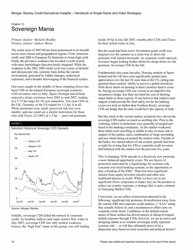
Morgan Stanley Credit Derivatives Insights – Handbook of Single Name and Index Strategies
74 Please see additional important disclosures at the end of this report.
Chapter 12
Sovereign Mania
Primary Analyst: Michelle Bradley Primary Analyst: Andrew Sheets
The credit crisis of 2007/08 has been pronounced in its breadth across asset classes and geographical regions. From American credit card ABS to European IG financials to Asian high yield bonds, the pervasive weakness has revealed a credit system with more interlinkages than previously imagined. While the weakness in the 2001-2002 credit cycle was a story of defaults and idiosyncratic risk, systemic fears define the current environment, generated by hidden linkages, undeclared exposures, and a broader deleveraging of the financial system.
One asset caught in the middle of these mingling forces has been CDS on developed European sovereign countries. CDS on names such as Italy, Spain, Portugal and Ireland enjoyed a sleepy existence from 2003 to mid-2007, trading in a 5-15 bp range for 10-year maturities. Ten-year CDS on the UK, Germany or the US traded for 1-2 bp, if at all. While premiums were small, perceived risk was even smaller, and one could see a similar motivation for those who sold iTraxx 22-100% at 1.5 bp — pure risk premium.
exhibit 1
Selected Historical Sovereign CDS Spreads
10yr Spread (bp)
0
10
20
30
40
50
60
Jun-02 Jun-03 Jun-04 Jun-05 Jun-06 Jun-07
Greece 10Y
Belgium 10Y
Italy 10Y
Spain 10Y
Source: Morgan Stanley
Initially, sovereign CDS faded the turmoil in corporate credit. As headline indices (and super senior) flew wider in July 2007, sovereign CDS saw only modest weakness. Greece, the “high beta” name in this group, was still trading
inside 20 bp in late fall 2007, months after CDX and iTraxx hit their initial wides in July.
But the seeds had been sown. Investment grade credit was targeted over the summer as a clean way to short risk premium with limited downside. As corporate credit repriced, investors began looking farther afield for cheap shorts on risk premium. Sovereign CDS fit the bill.
Fundamentals also came into play. Housing markets in Spain, Ireland and the UK have seen significantly greater price appreciation over the last 10 years than in the US, calling into question these markets’ ability to survive a global slowdown. With direct shorts on housing in these countries hard to come by, buying sovereign CDS was viewed as an imperfect but inexpensive hedge, less than one-third the cost of shorting major banks in these regions. If one believes that implicit state support would provide the final safety net for the banking sector (we look no further than Northern Rock), sovereign CDS can hedge that the state would have the capacity to help.
But like much in the current market, technicals have driven the sovereign CDS market as much as anything else. Prior to the widening, sellers of protection were generally leveraged and based in the banking community. As the market weakened, these banks were unwilling or unable to take on more risk in support of the market, and a combination of longs unwinding and new shorts being set pushed the market wider. Outside of the banks, few natural takers of risk existed; spreads had been so tight for so long that few EM or corporate credit investors had bothered with the market over the previous five years.
This is changing. With spreads in a decisively new postcode, a more balanced opportunity exists. We see buyers of protection motivated by a liquid hedge for systemic risk, concerns over local banking systems, or the opportunity to play a breakup of the EMU. There has been significant interest from equity investors (stocks) and other non-traditional players in credit. While we have yet to see significant flows, corporates or banks may use the product to reduce net country exposure, a strategy that is quite common in Emerging Market CDS.
Conversely, we see sellers of protection attracted to the following: significant risk premium, diversification away from the current ABS and corporate-credit malaise, a “AAA” rating they actually believe in, and a mechanism to offset carry on corporate credit shorts. Confidence in the default-remote nature of these entities has driven interest in taking leveraged default exposure through FTDs; however, we see an active and intriguing debate as to whether sovereigns really represent systemic risk — or will they ultimately prove to be a dispersion story based on local economic and political factors?

Section A, Chapter 12 Sovereign Mania
Please see additional important disclosures at the end of this report. 75
SOVEREIGN CDS CONTRACT SPECIFICS In most aspects, sovereign CDS is similar to the standard corporate CDS contract described in Chapter 1 of this book. But details are important, and we attempt to highlight salient features that distinguish the sovereign CDS contract. We note that the contract is fairly flexible and that much of the following is based on specifications investors make during the CDS confirmation at the time of the trade.
CURRENCY AND TENOR Ten-year CDS serves as the benchmark tenor for European sovereigns, rather than the 5-year point in corporate markets. In contrast to corporates, sovereign CDS is quoted in a non-native currency, so swaps on countries using the euro will trade in USD (while a CDS on the US will have cashflows in euros). Flexibility does exist in the marketplace to trade across currency types, which can be specified in the trade confirmation documentation.
DELIVERABLE OBLIGATIONS Reference Entity: Successor reference entity – direct or indirect successor, regardless of whether the successor assumes the obligations of the reference entity.
Reference Obligation: The reference obligation will be specified in the confirmation.
Characteristics of Deliverable Obligations:
• Maximum maturity (30-year), as of the physical settlement date
• Not bearer, although bearer bonds that are cleared via an internationally recognised clearing system are deliverable
• May not be contingent
• Convertible, exchangeable and accreting obligations are allowed so long as the rights have not been exercised before the delivery date
• May be transferable
• There is no contractual statutory or regulatory restriction to sale (144A and RegS do not count as restrictions to sale)
• Standard specified currencies: Canada, Japan, Switzerland, UK, US and the euro (and any successor to any such currency)
CREDIT EVENTS The following quality as credit events for sovereign CDS: • Bankruptcy • Failure to pay • Obligation acceleration • Obligation default • Repudiation/moratorium • Restructuring
Failure to Pay: If the reference entity fails to make a payment when the payment is due or fails to pay the entire amount due for one or more obligation, CDS is triggered.
Failure to pay either a redemption or coupon would qualify as an event of default, provided the failed amount in question is greater than US$1,000,000 (or as specified in the confirmation).
Exception to “Failure to Pay”: Grace Period – A grace period extension provides for the case when the end of the grace period runs beyond the termination date of the CDS. In this case, the grace period extension and hence the CDS protection will run beyond the termination date. This will be specified in the CDS confirmation.
Repudiation/Moratorium: The authorised authority refuses to pay some of the obligations outstanding or challenges its validity. Or, a moratorium is imposed whereby payment can be delayed or deferred. If a failure to pay or restructuring occurs as a result of the imposition of the repudiation/moratorium, this will trigger CDS. This is regardless of the payment or default requirement. Historical examples have been Mexico, Brazil, Argentina, and Russia’s 90-day debt moratorium.
Restructuring: One of the following events occur that changes the value of one or more obligation by more than the default requirement amount (this amount is discussed later). The event must be binding for all holders of such obligations and must be agreed upon between the government authority and a sufficient number of holders, or announced to be binding to all holders of such obligation. Qualifying events would be:
• Reduction in rate, interest payable or interest accruals
• Reduction in principal or premium payable at maturity or on scheduled redemption dates
• Postponement or deferral of interest, or the accrual of interest, or the payment of principal
• Change in the ranking of payment that would cause subordination
• Change in currency or composition of any interest or principal to a currency which is not a permitted currency. Permitted currency is either of the following:
(a) The legal tender of any G7 country: Canada, France, Germany, Italy, Japan, UK, US
(b) The legal tender of any OECD country that has a local currency long-term rating of “AAA” by Fitch, Moody’s, or Standard & Poor’s: Australia, Austria, Canada, Denmark, Finland, France, Germany, Iceland, Ireland, Luxembourg, Netherlands, New Zealand, Norway, Spain, Sweden, Switzerland, UK and US

Morgan Stanley Credit Derivatives Insights – Handbook of Single Name and Index Strategies
76 Please see additional important disclosures at the end of this report.
When is restructuring not an event of default?
1) If a state has adopted or adopts the euro and makes interest or principal payments in euros, this would not be considered a restructuring event.
Example – Poland joining the EMU and adopting the euro
2) If any stated restructuring events result from administrative adjustment, accounting adjustment, tax adjustment or any other technical adjustment occurring in the ordinary course of business.
Example – Change in tax legislation that affected coupon payments
3) If any of the restructuring events occur, but the events do not directly or indirectly result from a deterioration in the creditworthiness or financial condition of the reference entity.
Example – Sovereign refinances its debt, but in way beneficial to investors
Default requirement: The minimum amount of bonds on which the reference entity must default in order to trigger the contract. Specified in the confirmation; if not specified, US$10,000,000.
WHAT DOES AN EMU BREAK-UP MEAN FOR SOVEREIGN CDS? Sovereign CDS has generated significant investor interest as a way to position for a break-up of the EMU. Details here are important, as we can foresee a number of scenarios where, even if an EMU break-up does occur, protection buyers would be disappointed by the performance of their contracts.
If a country decides to leave the EMU and changes its legal tender, this does not necessarily imply that the current outstanding euro bonds would be re-denominated. As there is no treaty or provision for a country leaving the euro, a country could re-denominate its debt into its new currency, or it could leave the debt outstanding in euros. In a scenario where a country revalues its currency but leaves its debt in euros (for example, if it felt that it would deter investors by
re-denominating to a lower-valued currency), CDS would not be triggered.
Additionally, if debt were redenominated, this again would not necessarily trigger CDS. At issue is whether the new currency is part of the “G7” (Canada, France, Germany, Italy, Japan, UK, US). Below, we show a decision tree for navigating how leaving the EMU can impact CDS.
exhibit 2
Decision Tree for Sovereign CDS upon Leaving EMU
Source: Morgan Stanley
We use the following hypothetical scenario to illustrate this: Italy, Austria and Greece pull out of the European Union and each create a new legal tender. Would this be a restructuring event of default?
Italy: Not a credit event – Italy is a member of the G7, and hence Italy’s legal tender would be a permitted currency
Austria: Not a credit event – Austria is not a G7 country. But it is an OECD country and as long as it maintains its triple-A rating then the re-denomination would be into a permitted currency
Greece: Yes, a credit event – Greece is not a G7 country. It is an OECD country, but does not have a AAA rating. Therefore, the re-domination would not be in a permitted currency. However, as long as Greece keeps paying its outstanding euro debt in euros, CDS will not be triggered.
Country Leaves EMU
Re-Denominates Debt Leaves Debt in Euro
Is the Country G7 or Triple A OECD?
Doesn’t Trigger CDS
Permitted Currency
Doesn’t Trigger CDS
Not a Permitted Currency
Trigger CDS

Section B
Valuation and Investment Frameworks
Morgan Stanley Credit Derivatives Insights – Handbook of Single Name and Index Strategies
78 Please see additional important disclosures at the end of this report.
Chapter 13
Valuing Corporate Credit:Quantitative Approaches vs. Fundamental Analysis October 8, 2002
Primary Analyst: Sivan Mahadevan Primary Analyst: Young-Sup Lee Primary Analyst: David Schwartz Primary Analyst: Stephen Dulake Primary Analyst: Viktor Hjort
Introduction and Executive Summary INTRODUCTIONThe confluence of several major events in the credit markets has put a new focus on valuing corporate credit. First, the excesses of the 1990s equity bull market have created a harsh market environment, characterized by historically high default rates and investigations into the management and reporting of corporate balance sheets. Second, the rapid development of the credit derivatives market has brought together previously disparate credit markets and created the opportunity to trade credit risk in an isolated form. Third, the market for structured credit products such as CDOs has grown rapidly, with investors in these structures requiring a rigorous understanding of default risk within the context of a portfolio of correlated assets. Finally, speculators have entered the credit markets seeking to identify arbitrage opportunities and implement relative value strategies.
Given this evolution of the credit markets, what methodologies can be used to value corporate credit? There are many potential answers to this question. Quantitative approaches have gained popularity recently, particularly structural models based on equity market inputs. The traditional fundamental approach, used by most credit analysts, requires company and industry knowledge and has been in practice for decades, if not centuries.
In this chapter, we compare fundamental approaches to valuing corporate credit with quantitative approaches, commenting on their relative merits and predictive powers. On the quantitative front, we first review structural models, such as KMV and CreditGradesTM, which use information from the equity markets and corporate balance sheets to determine default probabilities or fair market spreads. Second, we describe reduced form models, which use information from the fixed income markets to directly model default probabilities. Third, we review simple statistical techniques such as factor models, which aid in determining relative value. With respect to fundamental approaches, we examine rating agency and credit analyst methodologies in detail.
KEY CONCLUSIONS We have drawn two sets of conclusions from this research effort. First, we summarize key points, both negative and positive, of various quantitative and fundamental approaches
to valuing credit described in this chapter. Second, in deciding which approach should be used, we conclude that the approaches are not mutually exclusive. Both structural models and traditional fundamental analysis require the same set of balance sheet inputs. In determining which approaches are applicable, both investor profile and the situation specific to a given credit should be considered. An investor’s choice of a technique can be related to mark-to-market requirements as well as the performance goals (relative to a benchmark versus absolute). With respect to a specific company, we feel it is important to consider three dimensions:
How far is the company from its default barrier? Structural approaches are less useful when companies are very close to the default barrier. In these cases, fundamental issues such as the likelihood of capital structure changes, possible corporate actions and potential changes in the business model are the real drivers of credit valuation. In structural models, the “distance to default” is the difference between a firm’s asset value and its liabilities, measured in units of the standard deviation of the asset value. Asset value is inferred from the equity markets.
How levered is the company? The importance of company-specific fundamental analysis increases as leverage levels rise because default is related to the success of the business model. We define leverage levels through metrics like debt-to-EBITDA ratios, which measure a company’s ability to service its debt from operations and are often included in a credit analyst’s valuation. This is distinct from the notion of distance to default in structural models defined above.
How likely is it that management significantly alters the capital structure of the company? An associated high probability should dominate valuation. Subjective views on the nature and timing of capital structure changes, if available from analysts, are very important in determining valuation. One framework for thinking about this “management option” is to analyze where a company lies along its weighted average cost of capital (WACC) curve. Quantitative approaches can help the credit expert understand the sensitivity of valuation to changes in the capital structure.
QUANTITATIVE APPROACHES: KEY POINTS • There have been many enhancements to Merton’s original
structural model, such as KMV and CreditGrades, which have been calibrated to produce realistic default probabilities and spreads. These models incorporate company-specific details and can include credit analyst projections.

Section B, Chapter 13 Valuing Corporate Credit: Quantitative Approaches vs. Fundamental Analysis
Please see additional important disclosures at the end of this report. 79
• Structural models are based on equity values and volatility. Equity markets are generally more liquid and transparent than corporate bond markets; however, if equity prices become irrationally inflated or deflated, they may be questionable indicators of actual asset values.
• In the structural framework, financial institutions should be modeled with caution, since it can be harder to assess their assets and liabilities.
• Reduced form models are calibrated using fixed income instruments, and do not rely on equity market information. They are well-suited for pricing credit derivatives and credit portfolio products, but do not reveal much new information about the securities used in the calibration.
FUNDAMENTAL APPROACHES: KEY POINTS • In some cases, there may no substitute for the credit expert
who can formulate subjective views on business, financial and strategic risks associated with a company or industry.
• In the fundamental approach, special considerations such as pension liabilities and off-balance-sheet items, which have been a focus in the market recently, can be easily incorporated in an analysis.
• The motivation for changing the capital structure of a company, and the likelihood of such a change occurring, can drive the valuation of corporate credit in a significant manner. Fundamental approaches allow for important subjective views on capital structure changes.
• Fundamental approaches do not directly lead to market prices. Valuations are usually made in a relative value context.
HISTORICAL EXPERIENCE: KEY POINTS • Based on our simple historical study, KMV Expected
Default FrequenciesTM (EDFTM) were good predictors of default and performed consistently over different categories of risk.
• In a similar study, market-implied default probabilities (i.e., using spread as a predictor) overestimated default in most cases, given risk premiums inherent in market spreads. Furthermore, they were inconsistent predictors of default at different risk levels.
• As a quantifiable measure of the performance of the fundamental approach, changes in free cash flow generation relative to debt were a good predictor of relative spread movements, based on our historical study.
• Over long periods of time for the market at large, actual ratings migration and default behavior have been consistent with ratings expectations from both Moody’s and S&P.
Quantitative Approaches to Valuing Corporate Credit Quantitative approaches for analyzing credit have existed for decades, but have surged in popularity over the last few years. This is due, in large part, to several trends in the credit markets:
• As credit spreads have widened and default rates have increased, investors have looked to increase their arsenal of tools for analyzing corporate bonds. Quantitative models can be used to provide warning signals or to determine whether the spread on a corporate bond adequately compensates the investor for the risk.
• The number of investors interested in credit products has grown worldwide. In part, this can be attributed to declining yields on competing investments and the expansion of the European corporate bond market following the introduction of the euro. Commercially available credit models have been developed to meet the growing investor demand.
• The rapidly expanding credit derivatives market, which includes credit default swaps and collateralized debt obligations, has spurred a new generation of quantitative models. For derivative products, quantitative techniques are critical for valuation and hedging.
• Risk management has become increasingly important for financial institutions. The need to compute “value at risk” and determine appropriate regulatory capital reserves has led to the development of sophisticated quantitative credit models.
In this section, we introduce some popular quantitative techniques for analyzing individual credits. (We discuss quantitative methods for portfolio products later in this publication.) The goal of these methods is to estimate default probabilities or fair market spreads. Although many different quantitative techniques are practiced in the market, we focus on two different approaches for modeling default: structural models and reduced form models. For comparison, we also review a simple factor model of corporate bond spreads.
• Structural models – These models use information from the equity market and corporate balance sheets to model a corporation’s assets and liabilities. Default occurs when the value of the corporation’s assets falls below its liabilities. Structural models are used to infer default probabilities and fair market spreads. KMV and CreditGrades are two commercial examples of this approach.
• Reduced form models – Unlike structural models, reduced form models rely on information from the fixed income market, such as asset swap spreads or default swap spreads. In these models, default probabilities are modeled directly, similar to the way interest rates are modeled for the purpose of pricing fixed income derivatives. These models
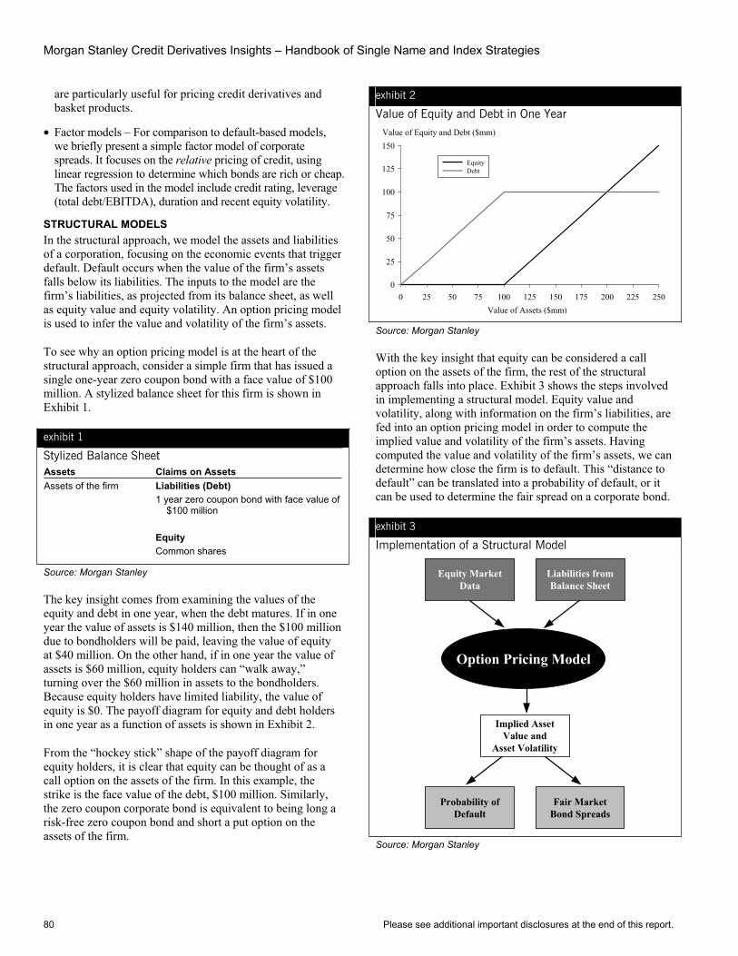
Morgan Stanley Credit Derivatives Insights – Handbook of Single Name and Index Strategies
80 Please see additional important disclosures at the end of this report.
are particularly useful for pricing credit derivatives and basket products.
• Factor models – For comparison to default-based models, we briefly present a simple factor model of corporate spreads. It focuses on the relative pricing of credit, using linear regression to determine which bonds are rich or cheap. The factors used in the model include credit rating, leverage (total debt/EBITDA), duration and recent equity volatility.
STRUCTURAL MODELS In the structural approach, we model the assets and liabilities of a corporation, focusing on the economic events that trigger default. Default occurs when the value of the firm’s assets falls below its liabilities. The inputs to the model are the firm’s liabilities, as projected from its balance sheet, as well as equity value and equity volatility. An option pricing model is used to infer the value and volatility of the firm’s assets.
To see why an option pricing model is at the heart of the structural approach, consider a simple firm that has issued a single one-year zero coupon bond with a face value of $100 million. A stylized balance sheet for this firm is shown in Exhibit 1.
exhibit 1
Stylized Balance Sheet Assets Claims on Assets Assets of the firm Liabilities (Debt) 1 year zero coupon bond with face value of
$100 million
Equity Common shares
Source: Morgan Stanley
The key insight comes from examining the values of the equity and debt in one year, when the debt matures. If in one year the value of assets is $140 million, then the $100 million due to bondholders will be paid, leaving the value of equity at $40 million. On the other hand, if in one year the value of assets is $60 million, equity holders can “walk away,” turning over the $60 million in assets to the bondholders. Because equity holders have limited liability, the value of equity is $0. The payoff diagram for equity and debt holders in one year as a function of assets is shown in Exhibit 2.
From the “hockey stick” shape of the payoff diagram for equity holders, it is clear that equity can be thought of as a call option on the assets of the firm. In this example, the strike is the face value of the debt, $100 million. Similarly, the zero coupon corporate bond is equivalent to being long a risk-free zero coupon bond and short a put option on the assets of the firm.
exhibit 2
Value of Equity and Debt in One Year Value of Equity and Debt ($mm)
0
25
50
75
100
125
150
0 25 50 75 100 125 150 175 200 225 250Value of Assets ($mm)
EquityDebt
Source: Morgan Stanley
With the key insight that equity can be considered a call option on the assets of the firm, the rest of the structural approach falls into place. Exhibit 3 shows the steps involved in implementing a structural model. Equity value and volatility, along with information on the firm’s liabilities, are fed into an option pricing model in order to compute the implied value and volatility of the firm’s assets. Having computed the value and volatility of the firm’s assets, we can determine how close the firm is to default. This “distance to default” can be translated into a probability of default, or it can be used to determine the fair spread on a corporate bond.
exhibit 3
Implementation of a Structural Model
Implied AssetValue and
Asset Volatility
Equity MarketData
Probability ofDefault
Liabilities fromBalance Sheet
Fair MarketBond Spreads
Option Pricing Model
Source: Morgan Stanley
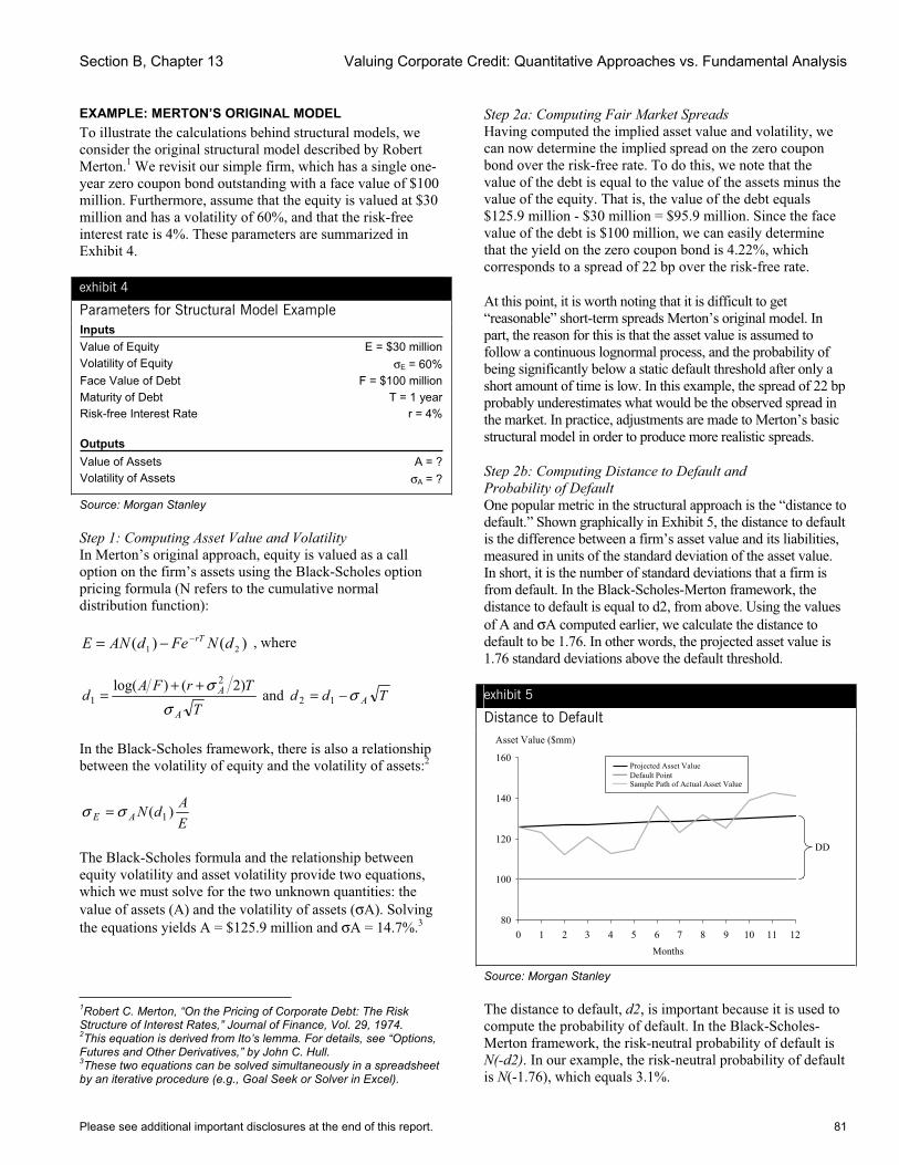
Section B, Chapter 13 Valuing Corporate Credit: Quantitative Approaches vs. Fundamental Analysis
Please see additional important disclosures at the end of this report. 81
EXAMPLE: MERTON’S ORIGINAL MODEL To illustrate the calculations behind structural models, we consider the original structural model described by Robert Merton.1 We revisit our simple firm, which has a single one-year zero coupon bond outstanding with a face value of $100 million. Furthermore, assume that the equity is valued at $30 million and has a volatility of 60%, and that the risk-free interest rate is 4%. These parameters are summarized in Exhibit 4.
exhibit 4
Parameters for Structural Model Example Inputs Value of Equity E = $30 millionVolatility of Equity σE = 60%Face Value of Debt F = $100 millionMaturity of Debt T = 1 yearRisk-free Interest Rate r = 4%
Outputs Value of Assets A = ?Volatility of Assets σA = ?
Source: Morgan Stanley
Step 1: Computing Asset Value and Volatility In Merton’s original approach, equity is valued as a call option on the firm’s assets using the Black-Scholes option pricing formula (N refers to the cumulative normal distribution function):
)()( 21 dNFedANE rT−−= , where
TTrFA
dA
A
σσ )2()log( 2
1++
= and Tdd Aσ−= 12
In the Black-Scholes framework, there is also a relationship between the volatility of equity and the volatility of assets:2
EAdNAE )( 1σσ =
The Black-Scholes formula and the relationship between equity volatility and asset volatility provide two equations, which we must solve for the two unknown quantities: the value of assets (A) and the volatility of assets (σA). Solving the equations yields A = $125.9 million and σA = 14.7%.3
1Robert C. Merton, “On the Pricing of Corporate Debt: The Risk Structure of Interest Rates,” Journal of Finance, Vol. 29, 1974. 2This equation is derived from Ito’s lemma. For details, see “Options, Futures and Other Derivatives,” by John C. Hull. 3These two equations can be solved simultaneously in a spreadsheet by an iterative procedure (e.g., Goal Seek or Solver in Excel).
Step 2a: Computing Fair Market Spreads Having computed the implied asset value and volatility, we can now determine the implied spread on the zero coupon bond over the risk-free rate. To do this, we note that the value of the debt is equal to the value of the assets minus the value of the equity. That is, the value of the debt equals $125.9 million - $30 million = $95.9 million. Since the face value of the debt is $100 million, we can easily determine that the yield on the zero coupon bond is 4.22%, which corresponds to a spread of 22 bp over the risk-free rate.
At this point, it is worth noting that it is difficult to get “reasonable” short-term spreads Merton’s original model. In part, the reason for this is that the asset value is assumed to follow a continuous lognormal process, and the probability of being significantly below a static default threshold after only a short amount of time is low. In this example, the spread of 22 bp probably underestimates what would be the observed spread in the market. In practice, adjustments are made to Merton’s basic structural model in order to produce more realistic spreads.
Step 2b: Computing Distance to Default and Probability of Default One popular metric in the structural approach is the “distance to default.” Shown graphically in Exhibit 5, the distance to default is the difference between a firm’s asset value and its liabilities, measured in units of the standard deviation of the asset value. In short, it is the number of standard deviations that a firm is from default. In the Black-Scholes-Merton framework, the distance to default is equal to d2, from above. Using the values of A and σA computed earlier, we calculate the distance to default to be 1.76. In other words, the projected asset value is 1.76 standard deviations above the default threshold.
exhibit 5
Distance to Default
80
100
120
140
160
0 1 2 3 4 5 6 7 8 9 10 11 12Months
Asset Value ($mm)
Projected Asset ValueDefault PointSample Path of Actual Asset Value
DD
Source: Morgan Stanley
The distance to default, d2, is important because it is used to compute the probability of default. In the Black-Scholes-Merton framework, the risk-neutral probability of default is N(-d2). In our example, the risk-neutral probability of default is N(-1.76), which equals 3.1%.
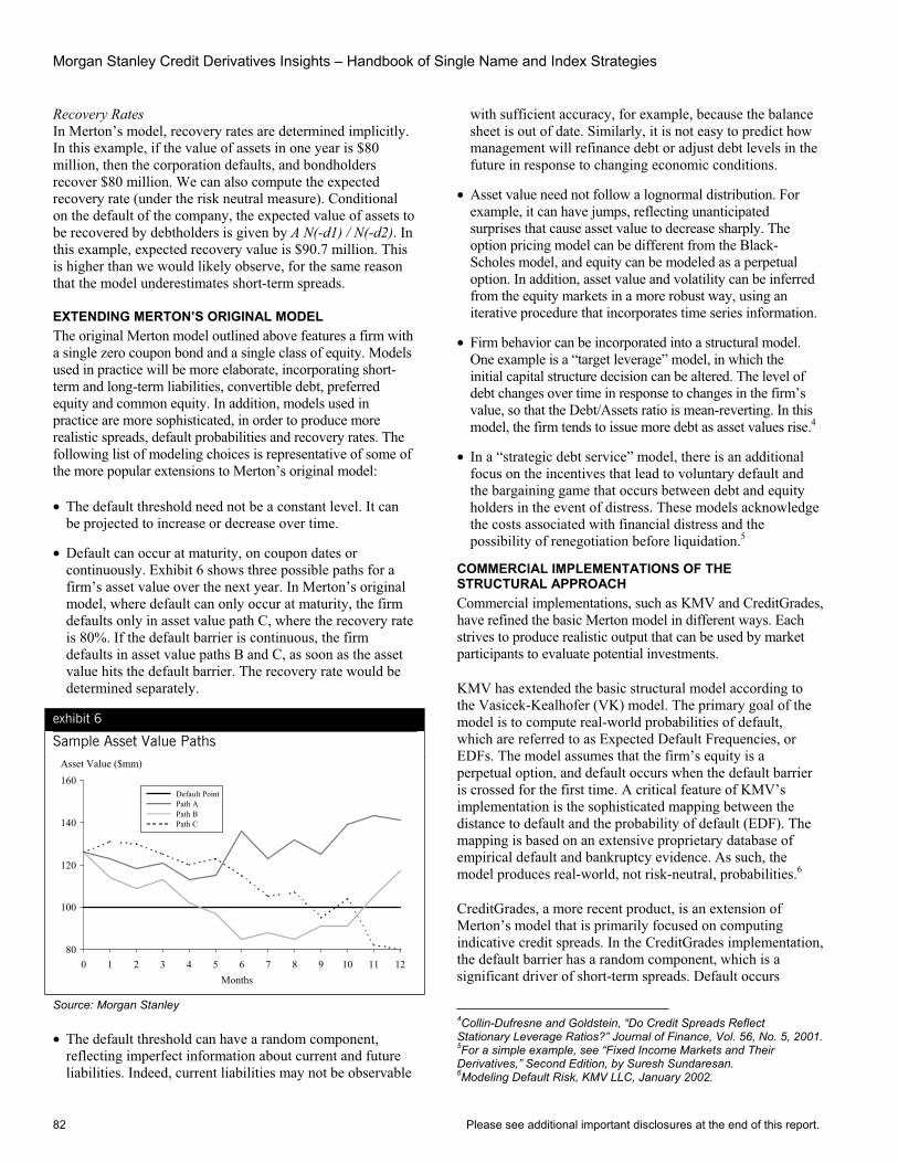
Morgan Stanley Credit Derivatives Insights – Handbook of Single Name and Index Strategies
82 Please see additional important disclosures at the end of this report.
Recovery Rates In Merton’s model, recovery rates are determined implicitly. In this example, if the value of assets in one year is $80 million, then the corporation defaults, and bondholders recover $80 million. We can also compute the expected recovery rate (under the risk neutral measure). Conditional on the default of the company, the expected value of assets to be recovered by debtholders is given by A N(-d1) / N(-d2). In this example, expected recovery value is $90.7 million. This is higher than we would likely observe, for the same reason that the model underestimates short-term spreads.
EXTENDING MERTON’S ORIGINAL MODEL The original Merton model outlined above features a firm with a single zero coupon bond and a single class of equity. Models used in practice will be more elaborate, incorporating short-term and long-term liabilities, convertible debt, preferred equity and common equity. In addition, models used in practice are more sophisticated, in order to produce more realistic spreads, default probabilities and recovery rates. The following list of modeling choices is representative of some of the more popular extensions to Merton’s original model:
• The default threshold need not be a constant level. It can be projected to increase or decrease over time.
• Default can occur at maturity, on coupon dates or continuously. Exhibit 6 shows three possible paths for a firm’s asset value over the next year. In Merton’s original model, where default can only occur at maturity, the firm defaults only in asset value path C, where the recovery rate is 80%. If the default barrier is continuous, the firm defaults in asset value paths B and C, as soon as the asset value hits the default barrier. The recovery rate would be determined separately.
exhibit 6
Sample Asset Value Paths
80
100
120
140
160
0 1 2 3 4 5 6 7 8 9 10 11 12Months
Asset Value ($mm)
Path B
Default PointPath A
Path C
Source: Morgan Stanley
• The default threshold can have a random component, reflecting imperfect information about current and future liabilities. Indeed, current liabilities may not be observable
with sufficient accuracy, for example, because the balance sheet is out of date. Similarly, it is not easy to predict how management will refinance debt or adjust debt levels in the future in response to changing economic conditions.
• Asset value need not follow a lognormal distribution. For example, it can have jumps, reflecting unanticipated surprises that cause asset value to decrease sharply. The option pricing model can be different from the Black-Scholes model, and equity can be modeled as a perpetual option. In addition, asset value and volatility can be inferred from the equity markets in a more robust way, using an iterative procedure that incorporates time series information.
• Firm behavior can be incorporated into a structural model. One example is a “target leverage” model, in which the initial capital structure decision can be altered. The level of debt changes over time in response to changes in the firm’s value, so that the Debt/Assets ratio is mean-reverting. In this model, the firm tends to issue more debt as asset values rise.4
• In a “strategic debt service” model, there is an additional focus on the incentives that lead to voluntary default and the bargaining game that occurs between debt and equity holders in the event of distress. These models acknowledge the costs associated with financial distress and the possibility of renegotiation before liquidation.5
COMMERCIAL IMPLEMENTATIONS OF THE STRUCTURAL APPROACH Commercial implementations, such as KMV and CreditGrades, have refined the basic Merton model in different ways. Each strives to produce realistic output that can be used by market participants to evaluate potential investments.
KMV has extended the basic structural model according to the Vasicek-Kealhofer (VK) model. The primary goal of the model is to compute real-world probabilities of default, which are referred to as Expected Default Frequencies, or EDFs. The model assumes that the firm’s equity is a perpetual option, and default occurs when the default barrier is crossed for the first time. A critical feature of KMV’s implementation is the sophisticated mapping between the distance to default and the probability of default (EDF). The mapping is based on an extensive proprietary database of empirical default and bankruptcy evidence. As such, the model produces real-world, not risk-neutral, probabilities.6
CreditGrades, a more recent product, is an extension of Merton’s model that is primarily focused on computing indicative credit spreads. In the CreditGrades implementation, the default barrier has a random component, which is a significant driver of short-term spreads. Default occurs
4Collin-Dufresne and Goldstein, “Do Credit Spreads Reflect Stationary Leverage Ratios?” Journal of Finance, Vol. 56, No. 5, 2001. 5For a simple example, see “Fixed Income Markets and Their Derivatives,” Second Edition, by Suresh Sundaresan. 6Modeling Default Risk, KMV LLC, January 2002.

Section B, Chapter 13 Valuing Corporate Credit: Quantitative Approaches vs. Fundamental Analysis
Please see additional important disclosures at the end of this report. 83
whenever the default threshold is crossed for the first time. Parameters for the model have been estimated in order to achieve consistency with historical default swap spreads.7
ADVANTAGES OF STRUCTURAL MODELS • Equity markets are generally more liquid and transparent
than corporate bond markets, and some argue that they provide more reliable information. Using equity market information allows fixed income instruments to be priced independently, without requiring credit spread information from related fixed income instruments.
• Structural models attempt to explain default from an economic perspective. They are oriented toward the fundamentals of the company, focusing on its balance sheet and asset value.
• Credit analysts’ forecasts can be incorporated into the model to enhance the quality of its output. For example, balance sheet projections can be used to create a more realistic default threshold. The model can also be run under different scenarios for future liabilities.
• Structural models are well-suited for handling different securities of the same issuer, including bonds of various seniorities and convertible bonds.
• A variety of structural models are commercially available. They can be used as a screening tool for large portfolios, especially when credit analyst resources are limited.
• Structural models can be enhanced, for example, to incorporate firm behavior. Examples include target leverage models and strategic debt service models.
• Default correlation can be modeled quite naturally in the structural framework. In a portfolio context, correlation in asset values drives default correlation.
DISADVANTAGES OF STRUCTURAL MODELS • If equity prices become irrationally inflated, they may be
poor indicators of actual asset value. The Internet and telecom bubbles of the past few years are perhaps the most striking examples. Generally, users of structural models must believe that they can reasonably imply asset values from equity market information. This can become a significant issue when current earnings are low or negative and equity valuations are high.
• Bond prices and credit default swap spreads, which arguably contain valuable information about the probability of default, are outputs of the model, not inputs.
• In Merton’s structural model, implied credit spreads on short-term debt and very high quality debt are very low when compared to empirical data. Refinements to the model have alleviated this problem, at the expense of simplicity.
7CreditGrades Technical Document, RiskMetrics Group, Inc., May 2002.
• The determination of a unique arbitrage-free option price implicitly assumes that the value of the whole firm is tradable and available as a hedge instrument, which is a questionable assumption. In addition, it may not be clear how to best model a firm’s asset value.
• Structural models can be difficult to calibrate. In practice, asset values and volatilities are best calibrated using time series information. Assumptions for equity volatility can have a significant impact on the model.
• Structural models can be complex, depending on the capital structure of the issuer and the level of detail captured by the model. An issuer may have multiple classes of short-term and long-term debt, convertible bonds, preferred shares and common equity.
• It can be difficult to get reliable, current data on a firm’s liabilities. Issues regarding transparency and accounting treatment are, of course, not unique to structural models. In addition, once adequate information on the liabilities is obtained, the information must be consolidated to project a default barrier.
• Notwithstanding innovations such as target leverage models and strategic debt service models, it is difficult to model future corporate behavior.
• It can be difficult to model a firm that is close to its default threshold, since firms will often adjust their liabilities as they near default. Firms will vary in terms of their ability to adjust their leverage as they begin to encounter difficulties. (For this reason, KMV reports a maximum EDF of 20%.)
• Financial institutions should be modeled with caution, since it can be harder to assess their assets and liabilities. In addition, since financial institutions are highly regulated, default may not be the point where the value of assets falls below the firm’s liabilities.
• Structural models are generally inappropriate for sovereign issuers.
REDUCED FORM MODELS In the reduced form approach, default is modeled as a surprise event. Rather than modeling the value of a firm’s assets, here we directly model the probability of default. This approach is similar to the way interest rates are modeled for the purpose of pricing fixed income derivatives. Unlike the structural models described above, the inputs for reduced form models come from the fixed income markets in the form of default swap spreads or asset swap spreads.
The quantity we are actually modeling in the reduced form approach is called the hazard rate, which we denote by h(t).The hazard rate is a forward probability of default, similar to a forward interest rate. The hazard rate has the following interpretation: given that a firm survives until time t, h(t)Δt
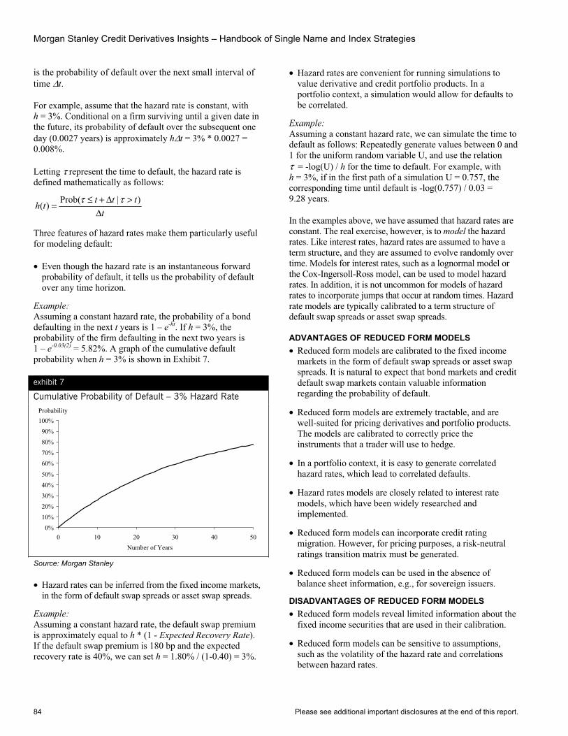
Morgan Stanley Credit Derivatives Insights – Handbook of Single Name and Index Strategies
84 Please see additional important disclosures at the end of this report.
is the probability of default over the next small interval of time Δt.
For example, assume that the hazard rate is constant, with h = 3%. Conditional on a firm surviving until a given date in the future, its probability of default over the subsequent one day (0.0027 years) is approximately hΔt = 3% * 0.0027 = 0.008%.
Letting τ represent the time to default, the hazard rate is defined mathematically as follows:
ttttth
Δ>Δ+≤
=)|(Prob)( ττ
Three features of hazard rates make them particularly useful for modeling default:
• Even though the hazard rate is an instantaneous forward probability of default, it tells us the probability of default over any time horizon.
Example:Assuming a constant hazard rate, the probability of a bond defaulting in the next t years is 1 – e-ht. If h = 3%, the probability of the firm defaulting in the next two years is 1 – e-0.03(2) = 5.82%. A graph of the cumulative default probability when h = 3% is shown in Exhibit 7.
exhibit 7
Cumulative Probability of Default – 3% Hazard Rate
0%10%20%30%40%50%
60%70%80%90%
100%
0 10 20 30 40 50Number of Years
Probability
Source: Morgan Stanley
• Hazard rates can be inferred from the fixed income markets, in the form of default swap spreads or asset swap spreads.
Example:Assuming a constant hazard rate, the default swap premium is approximately equal to h * (1 - Expected Recovery Rate). If the default swap premium is 180 bp and the expected recovery rate is 40%, we can set h = 1.80% / (1-0.40) = 3%.
• Hazard rates are convenient for running simulations to value derivative and credit portfolio products. In a portfolio context, a simulation would allow for defaults to be correlated.
Example:Assuming a constant hazard rate, we can simulate the time to default as follows: Repeatedly generate values between 0 and 1 for the uniform random variable U, and use the relation τ = -log(U) / h for the time to default. For example, with h = 3%, if in the first path of a simulation U = 0.757, the corresponding time until default is -log(0.757) / 0.03 = 9.28 years.
In the examples above, we have assumed that hazard rates are constant. The real exercise, however, is to model the hazard rates. Like interest rates, hazard rates are assumed to have a term structure, and they are assumed to evolve randomly over time. Models for interest rates, such as a lognormal model or the Cox-Ingersoll-Ross model, can be used to model hazard rates. In addition, it is not uncommon for models of hazard rates to incorporate jumps that occur at random times. Hazard rate models are typically calibrated to a term structure of default swap spreads or asset swap spreads.
ADVANTAGES OF REDUCED FORM MODELS • Reduced form models are calibrated to the fixed income
markets in the form of default swap spreads or asset swap spreads. It is natural to expect that bond markets and credit default swap markets contain valuable information regarding the probability of default.
• Reduced form models are extremely tractable, and are well-suited for pricing derivatives and portfolio products. The models are calibrated to correctly price the instruments that a trader will use to hedge.
• In a portfolio context, it is easy to generate correlated hazard rates, which lead to correlated defaults.
• Hazard rates models are closely related to interest rate models, which have been widely researched and implemented.
• Reduced form models can incorporate credit rating migration. However, for pricing purposes, a risk-neutral ratings transition matrix must be generated.
• Reduced form models can be used in the absence of balance sheet information, e.g., for sovereign issuers.
DISADVANTAGES OF REDUCED FORM MODELS • Reduced form models reveal limited information about the
fixed income securities that are used in their calibration.
• Reduced form models can be sensitive to assumptions, such as the volatility of the hazard rate and correlations between hazard rates.
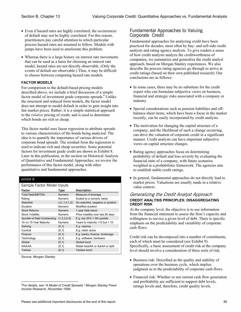
Section B, Chapter 13 Valuing Corporate Credit: Quantitative Approaches vs. Fundamental Analysis
Please see additional important disclosures at the end of this report. 85
• Even if hazard rates are highly correlated, the occurrences of default may not be highly correlated. For this reason, practitioners pay careful attention to which particular process hazard rates are assumed to follow. Models with jumps have been used to ameliorate this problem.
• Whereas there is a large history on interest rate movements that can be used as a basis for choosing an interest rate model, hazard rates are not directly observable. (Only the events of default are observable.) Thus, it may be difficult to choose between competing hazard rate models.
FACTOR MODELS For comparison to the default-based pricing models described above, we include a brief discussion of a simple factor model of investment grade corporate spreads.8 Unlike the structural and reduced form models, the factor model does not attempt to model default in order to gain insight into fair market prices. Rather, it is a simple statistical approach to the relative pricing of credit, and is used to determine which bonds are rich or cheap.
This factor model uses linear regression to attribute spreads to various characteristics of the bonds being analyzed. The idea is to quantify the importance of various drivers of corporate bond spreads. The residual from the regression is used to indicate rich and cheap securities. Some potential factors for investment grade credit are shown in Exhibit 8. Later in this publication, in the section on Historical Analysis of Quantitative and Fundamental Approaches, we review the performance of this factor model, along with other quantitative and fundamental approaches.
exhibit 8
Sample Factor Model Inputs Factor Type Description Total Debt/EBITDA Numeric Measure of leverage Rating Numeric Scaled to a numeric value Watchlist {-2,-1,0,1,2} On watchlist, negative or positive Duration Numeric Modified duration Stock Returns Numeric 1 year total return Stock Volatility Numeric Price volatility over last 90 days Quintile of Debt Outstanding {1,2,3,4,5} E.g. top 20% = 5th quintile 10- to 15-Year Maturity Numeric Years to maturity >10 but < 15 Gaming {0,1} E.g. casinos Cyclical {0,1} E.g. retail, autos Finance {0,1} E.g. banks, finance, brokerage Technology {0,1} E.g. software, hardware Global {0,1} Global bond AAA/AA {0,1} Rated Aaa/AA or Aa/AA or split Yankee {0,1} Yankee bond
Source: Morgan Stanley
8For details, see “A Model of Credit Spreads,” Morgan Stanley Fixed Income Research, November 1999.
Fundamental Approaches to Valuing Corporate Credit Fundamental approaches for analyzing credit have been practiced for decades, most often by buy- and sell-side credit analysts and rating agency analysts. To give readers a sense of how credit analysts analyze the creditworthiness of companies, we summarize and generalize the credit analyst approach, based on Morgan Stanley experiences. We also describe the process rating agencies go through to arrive at credit ratings (based on their own published research). Our conclusions are as follows:
• In some cases, there may be no substitute for the credit expert who can formulate subjective views on business, financial and strategic risks associated with a company or industry.
• Special considerations such as pension liabilities and off-balance-sheet items, which have been a focus in the market recently, can be easily incorporated by credit analysts.
• The motivation for changing the capital structure of a company, and the likelihood of such a change occurring, can drive the valuation of corporate credit in a significant manner. Credit analysts can have important subjective views on capital structure changes.
• Rating agency approaches focus on determining probability of default and loss severity by evaluating the financial state of a company, with future scenarios weighted in a probabilistic framework. The agencies aim to establish stable credit ratings.
• In general, fundamental approaches do not directly lead to market prices. Valuations are usually made in a relative value context.
Generalizing the Credit Analyst Approach CREDIT ANALYSIS PRINCIPLES: DISAGGREGATING CREDIT RISK At the company level, the objective is to use information from the financial statement to assess the firm’s capacity and willingness to service a given level of debt. There is specific emphasis on the predictability and variability of corporate cash flows.
Credit risk can be decomposed into a number of constituents, each of which must be considered (see Exhibit 9). Specifically, a basic assessment of credit risk at the company level should involve a consideration of three sorts of risk.
• Business risk: Described as the quality and stability of operations over the business cycle, which implies judgment as to the predictability of corporate cash flows.
• Financial risk: Whether or not current cash flow generation and profitability are sufficient to support debt levels, ratings levels and, therefore, credit quality levels.
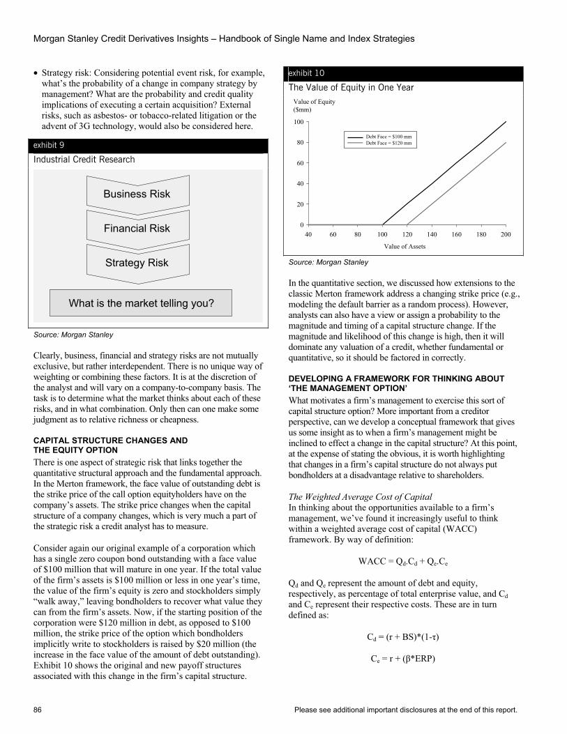
Morgan Stanley Credit Derivatives Insights – Handbook of Single Name and Index Strategies
86 Please see additional important disclosures at the end of this report.
• Strategy risk: Considering potential event risk, for example, what’s the probability of a change in company strategy by management? What are the probability and credit quality implications of executing a certain acquisition? External risks, such as asbestos- or tobacco-related litigation or the advent of 3G technology, would also be considered here.
exhibit 9
Industrial Credit Research
Business Risk
Financial Risk
Strategy Risk
What is the market telling you?
Source: Morgan Stanley
Clearly, business, financial and strategy risks are not mutually exclusive, but rather interdependent. There is no unique way of weighting or combining these factors. It is at the discretion of the analyst and will vary on a company-to-company basis. The task is to determine what the market thinks about each of these risks, and in what combination. Only then can one make some judgment as to relative richness or cheapness.
CAPITAL STRUCTURE CHANGES AND THE EQUITY OPTION There is one aspect of strategic risk that links together the quantitative structural approach and the fundamental approach. In the Merton framework, the face value of outstanding debt is the strike price of the call option equityholders have on the company’s assets. The strike price changes when the capital structure of a company changes, which is very much a part of the strategic risk a credit analyst has to measure.
Consider again our original example of a corporation which has a single zero coupon bond outstanding with a face value of $100 million that will mature in one year. If the total value of the firm’s assets is $100 million or less in one year’s time, the value of the firm’s equity is zero and stockholders simply “walk away,” leaving bondholders to recover what value they can from the firm’s assets. Now, if the starting position of the corporation were $120 million in debt, as opposed to $100 million, the strike price of the option which bondholders implicitly write to stockholders is raised by $20 million (the increase in the face value of the amount of debt outstanding). Exhibit 10 shows the original and new payoff structures associated with this change in the firm’s capital structure.
exhibit 10
The Value of Equity in One Year
0
20
40
60
80
100
40 60 80 100 120 140 160 180 200
Value of Assets
Value of Equity($mm)
Debt Face = $120 mmDebt Face = $100 mm
Source: Morgan Stanley
In the quantitative section, we discussed how extensions to the classic Merton framework address a changing strike price (e.g., modeling the default barrier as a random process). However, analysts can also have a view or assign a probability to the magnitude and timing of a capital structure change. If the magnitude and likelihood of this change is high, then it will dominate any valuation of a credit, whether fundamental or quantitative, so it should be factored in correctly.
DEVELOPING A FRAMEWORK FOR THINKING ABOUT ‘THE MANAGEMENT OPTION’ What motivates a firm’s management to exercise this sort of capital structure option? More important from a creditor perspective, can we develop a conceptual framework that gives us some insight as to when a firm’s management might be inclined to effect a change in the capital structure? At this point, at the expense of stating the obvious, it is worth highlighting that changes in a firm’s capital structure do not always put bondholders at a disadvantage relative to shareholders.
The Weighted Average Cost of Capital In thinking about the opportunities available to a firm’s management, we’ve found it increasingly useful to think within a weighted average cost of capital (WACC) framework. By way of definition:
WACC = Qd.Cd + Qe.Ce
Qd and Qe represent the amount of debt and equity, respectively, as percentage of total enterprise value, and Cdand Ce represent their respective costs. These are in turn defined as:
Cd = (r + BS)*(1- )
Ce = r + ( *ERP)

Section B, Chapter 13 Valuing Corporate Credit: Quantitative Approaches vs. Fundamental Analysis
Please see additional important disclosures at the end of this report. 87
Here, r is the risk-free rate (or benchmark government bond yield), BS is the borrowing spread on top of the risk-free rate, is the corporate tax rate, is a measure of the volatility of
the company’s stock vis-à-vis the broader equity market, and ERP is the market-wide equity risk premium.
Mapping the WACC to credit ratings, one would typically expect to observe the “hockey stick” profile shown in Exhibit 11. Remember, interest is tax deductible and dividends are only distributed after taxes. This is why, as more debt is added to the balance sheet and the firm migrates down the ratings spectrum, we initially observe a negatively-sloped WACC curve. Beyond a certain point, however, the incremental tax benefit associated with adding more debt to the balance sheet is more than offset by a combination of a higher borrowing spread and a rising .Thus, when we map the WACC to leverage and credit ratings, we observe an eventual shift from a negatively-sloped to a positively-sloped curve.
exhibit 11
A Stylized Version of the Weighted Average Cost of Capital
0
20
40
60
80
100
40 60 80 100 120 140 160 180 200
Value of Assets
Value of Equity($mm)
Debt Face = $120 mmDebt Face = $100 mm
Source: Morgan Stanley
The WACC is a theoretical concept, but it provides an extremely useful framework for thinking about the circumstances in which management might change the firm’s capital structure. A WACC framework helps us put bounds on the risk-reward structure associated with the “management option.” Specifically, we believe that it is at the tails of the leverage distribution where the risk-reward mismatch associated with a change in the capital structure is greatest, and therefore the incentive to change the capital structure is arguably the greatest. For example, at the high-end of the ratings spectrum, there is a strong incentive for a company to increase leverage and lower its cost of capital. Similarly, the incentive to pursue a strategy of balance sheet reparation is much stronger at the opposite end of the leverage distribution.
THE OPERATING ENVIRONMENT: INDUSTRY ANALYSIS Any fundamental assessment of corporate credit risk for a given company must necessarily extend beyond the latest set
of financials and consider the ‘macro’ operating environment including issues related to industry structure and evolution, the regulatory environment and barriers to entry.
To illustrate the questions that one will typically ask, it is important to consider whether, for example, we are dealing with a monopoly or a highly competitive business from an industry structure perspective. Barriers to entry have clear implications for pricing and earnings power. Is the business global or regional? For example, in the case of autos, what is the viability of a regional car maker in a global business?
On the regulatory front, deregulation has been a clear driver of capital structure and credit quality trends in the utility sector. Again, what is important from a credit risk perspective are the ex ante and ex post implications of any regulatory change on pricing power and the ability for a company to generate cash flow and support a given level of debt and credit quality.
exhibit 12
Forces Shaping the Operating Environment
Industry Structure
Industry Evolution
Regulation/De-regulation
Barriers to Entry
Global/Regional
Cyclicality
Industry Analysis
Source: Morgan Stanley
Regarding industry evolution, a classic case in point is the telecommunications business and the advent of 3G technology. As has been the case with deregulation in the utility sector, 3G has been the principal driver of the telecom credit quality rollercoaster of the past two years.
THE OUTPUT FROM CREDIT ANALYSTS: DETERMINING RELATIVE VALUE AND SPREADS At this point, a natural question to ask is how credit analysts translate their company-specific analyses into a spread? In our experience, we find that credit analysts formulate appropriate valuation levels through a relative value framework based on comparability. Such a framework takes the current market level for spreads as given, and suggests valuations through a peer group of comparable credits. Statements such as “company X should trade 20 bp behind company Y” are common, however subjective they may appear. We explore the importance of ratings versus sectors in determining these peer groups in the next section.

Morgan Stanley Credit Derivatives Insights – Handbook of Single Name and Index Strategies
88 Please see additional important disclosures at the end of this report.
exhibit 13
Single As – Sector Correlation Coefficients Based on Weekly Asset Swap Spread Changes End-1999 to Present Banks Non Bank Fins Con Disc Con Staples Energy Industrials Technology Telecoms UtilitiesBanks 1Non Bank Fins 0.55 1 Con Disc 0.41 0.59 1Con Staples 0.23 0.24 0.33 1 Energy 0.30 0.32 0.33 0.23 1Industrials 0.26 0.30 0.44 0.21 0.33 1 Technology 0.10 0.01 0.11 0.13 0.16 -0.04 1Telecoms 0.17 0.11 0.40 0.22 0.12 0.22 0.37 1Utilities 0.44 0.45 0.37 0.41 0.31 0.36 0.11 0.31 1
Source: Moody’s
exhibit 14
Telecoms – Cross-Credit Correlation Coefficients VOD TELECO OTE BRITEL FRTEL DT TIIM OLIVET KPNVOD 1TELECO 0.29 1 OTE 0.21 0.31 1BRITEL 0.54 0.04 0.37 1 FRTEL 0.47 0.13 0.48 0.68 1DT 0.41 -0.17 0.39 0.66 0.83 1 TIIM 0.60 0.39 0.35 0.61 0.60 0.44 1OLIVET 0.53 0.49 0.20 0.33 0.25 0.06 0.77 1KPN 0.33 0.23 0.39 0.36 0.58 0.39 0.53 0.38 1
Source: Morgan Stanley
COMPARABILITY: SECTORS VS. RATINGS Given the focus by credit analysts on identifying and utilizing an appropriate peer group for determining spreads, how should such a group of comparable credits be constructed? As an example, in Exhibit 13 we present inter-sector correlation coefficients for single-A rated segments of MSCI’s Euro Corporate Credit Index. The average pairwise correlation coefficient of weekly changes in asset swap spreads is 0.28, quite low in our opinion. Similarly, for BBB-rated corporate bonds (not shown), the average pairwise correlation coefficient is 0.24. From this analysis we can conclude that peer groupings based purely on credit ratings may not be appropriate.
What is the degree of correlation within a given sector between different credits with different ratings? We have focused our example on two of the more liquid sectors in the European credit markets, autos and telecommunications. Exhibit 15 presents the results of this exercise for the auto sector. We have selected five credits rated mid-A to mid-BBB with relatively liquid bonds of similar maturities outstanding. The lowest pair-wise correlation in the auto sector, at 0.31 between Ford and Renault, is higher than the average observed for either single As or triple Bs (see Exhibit 15). The average pair-wise correlation for the auto sector is 0.62, which would suggest that sector groupings are more important than ratings groups, at least when considering the auto sector.
The results for the telecom sector are shown in Exhibit 14. Again we have selected a group of credits that cover a reasonable spectrum of European credits. The average pair-wise correlation for the telecom sector is 0.40, which is again higher than that observed between different sectors within a given rating class.
exhibit 15
Autos – Cross-Credit Correlation Coefficients GM DCX FIAT RENAUL FGM 1DCX 0.84 1 FIAT 0.80 0.67 1RENAUL 0.34 0.42 0.50 1F 0.82 0.77 0.73 0.31 1
Source: Morgan Stanley
Section B, Chapter 13 Valuing Corporate Credit: Quantitative Approaches vs. Fundamental Analysis
Please see additional important disclosures at the end of this report. 89
Rating Agency Approaches No institution wields anywhere near as much influence on how the market perceives the credit quality of an individual borrower as the credit rating agencies. The agencies themselves see their role as being the providers of truly independent credit opinions, and as such, helping to overcome the information asymmetry between borrowers and lenders. With such monumental influence on pricing decisions, rating agencies, unsurprisingly, regularly receive criticism for not achieving all of their aims. Market participants have traditionally criticized the agencies for being too slow to react to new information. Lately the criticism has tended to be that agencies are too quick to change opinions. Nevertheless, given the crucial role the agencies play in the capital markets, it is important to understand the rating process and the factors that influence the agencies’ decisions.9
REDUCING INFORMATION ASYMMETRY Corporate borrowers have access to more detailed information on their businesses and credit profiles than do lenders. This is particularly true for capital market lenders. For commercial banks, which work closely with their clients, lending decisions are based on a detailed understanding of the borrowers. The process of lending is characterized by constant monitoring of credit quality and actively using covenants to restrict potentially credit-detrimental activities of borrowers. Ultimately, banks can agree to restructure loans as a final attempt to recover funds before allowing default.
The capital markets, on the other hand, are anonymous to the borrowers in the sense that borrowers will never know nor control who ultimately lent them the money. Precisely because of this distance between borrowers and lenders, bond investors rely on credit analysts to bridge the information asymmetry.
ARRIVING AT A RATING Credit rating agencies try to assess the probability of default and loss severity. The product of the two yields the expected loss. Based on this, a rating is produced. The rating is expected, over time, to map to a subsequent expected loss, based on historical experience. The process involves three main steps:
• Evaluating the financial status: Observing hard facts associated with the financial state of a particular company.
• Evaluating management: Subjectively evaluating the ability and interest in maintaining a particular credit profile.
• Conducting scenario analysis: Making assumptions about the probability of various scenarios that may impact the future credit profile.
Finally, arriving at a particular rating requires anchoring the two components, default probability and loss severity, to the historical experience. In estimating the default probability,
9For a more comprehensive survey, see Euro Credit Basis Report: “What’s Going on at the Rating Agencies?” Morgan Stanley Fixed Income Research, May 31, 2002.
rating agencies target relative risk over time. In estimating loss severity, analysts evaluate security and seniority, as well as sector differences. In addition, recovery rates may differ over time and across jurisdictions.
CREDITWORTHINESS IS A STABLE CONCEPT Underlying this process lies a crucial assumption: creditworthiness is a stable concept. Fundamentally, creditworthiness changes only gradually over time or at least is only confirmed over time. In theory, this ought to make multi-notch rating changes unlikely, and the rating agencies therefore use tools such as outlooks and watch lists to flag changes. Even these, however, tend to have a built-in lag. Moody’s, for instance, has an 18-month horizon for its outlooks and 90 days for its Watch List, whereas S&P targets 90 days for its CreditWatch listings, with a longer but unspecified time-horizon for Outlooks. This gradual approach gives credit ratings a serially correlated pattern. This is also what creates the impression that ratings activity lags the market so significantly.
HAVE THE AGENCIES CHANGED THEIR APPROACH? The rating agencies have been criticized for the market-lagging approach and serially correlated ratings pattern. The main criticism is that the approach causes ratings to lag their information content, and therefore lose their value as investor protection. In the case of Enron, for example, senior bonds and loans were already trading below 20 cents to the dollar when the company was downgraded to non-investment grade, which was less than a week before the company filed for Chapter 11 bankruptcy protection.
In response to this criticism, Moody’s put its ratings process under review early in 2002. Moody’s asked investors whether they wanted ratings decisions to be quicker and more severe. The use of so-called market-based tools for evaluating credit was also suggested. The answer to the consultation was overwhelmingly “no.” Investors showed little interest for a quicker ratings process, nor did they show any interest in the use of market-based tools to enhance the process. What there was a need for, according to the published feedback, was transparency.10
Standard & Poor’s, has not (publicly) put its process up for review, but has increasingly focused on issues that will enhance and complement the information content of the ratings. In particular, S&P has (i) begun surveying its corporate issuers for information on ratings contingent commitments, such as ratings triggers; (ii) indicated that it will start rating the transparency, disclosure and corporate governance practices of the companies in the S&P 500; (iii) introduced Core Earnings, a concept reflecting the agency’s belief of how fundamental earnings performance should be reflected; and (iv) introduced liquidity reports on individual companies.11
10Understanding Moody’s Corporate Bond Ratings and Ratings Process, Moody’s, May 2002. 11Enhancing Financial Transparency: The View from Standard & Poor’s, S&P, July 2002.
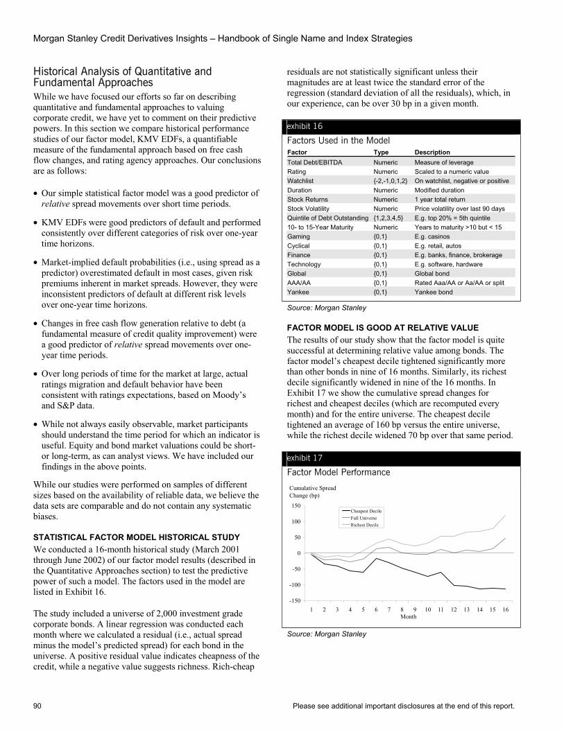
Morgan Stanley Credit Derivatives Insights – Handbook of Single Name and Index Strategies
90 Please see additional important disclosures at the end of this report.
Historical Analysis of Quantitative and Fundamental Approaches While we have focused our efforts so far on describing quantitative and fundamental approaches to valuing corporate credit, we have yet to comment on their predictive powers. In this section we compare historical performance studies of our factor model, KMV EDFs, a quantifiable measure of the fundamental approach based on free cash flow changes, and rating agency approaches. Our conclusions are as follows:
• Our simple statistical factor model was a good predictor of relative spread movements over short time periods.
• KMV EDFs were good predictors of default and performed consistently over different categories of risk over one-year time horizons.
• Market-implied default probabilities (i.e., using spread as a predictor) overestimated default in most cases, given risk premiums inherent in market spreads. However, they were inconsistent predictors of default at different risk levels over one-year time horizons.
• Changes in free cash flow generation relative to debt (a fundamental measure of credit quality improvement) were a good predictor of relative spread movements over one-year time periods.
• Over long periods of time for the market at large, actual ratings migration and default behavior have been consistent with ratings expectations, based on Moody’s and S&P data.
• While not always easily observable, market participants should understand the time period for which an indicator is useful. Equity and bond market valuations could be short- or long-term, as can analyst views. We have included our findings in the above points.
While our studies were performed on samples of different sizes based on the availability of reliable data, we believe the data sets are comparable and do not contain any systematic biases.
STATISTICAL FACTOR MODEL HISTORICAL STUDY We conducted a 16-month historical study (March 2001 through June 2002) of our factor model results (described in the Quantitative Approaches section) to test the predictive power of such a model. The factors used in the model are listed in Exhibit 16.
The study included a universe of 2,000 investment grade corporate bonds. A linear regression was conducted each month where we calculated a residual (i.e., actual spread minus the model’s predicted spread) for each bond in the universe. A positive residual value indicates cheapness of the credit, while a negative value suggests richness. Rich-cheap
residuals are not statistically significant unless their magnitudes are at least twice the standard error of the regression (standard deviation of all the residuals), which, in our experience, can be over 30 bp in a given month.
exhibit 16
Factors Used in the Model Factor Type Description Total Debt/EBITDA Numeric Measure of leverage Rating Numeric Scaled to a numeric value Watchlist {-2,-1,0,1,2} On watchlist, negative or positive Duration Numeric Modified duration Stock Returns Numeric 1 year total return Stock Volatility Numeric Price volatility over last 90 days Quintile of Debt Outstanding {1,2,3,4,5} E.g. top 20% = 5th quintile 10- to 15-Year Maturity Numeric Years to maturity >10 but < 15 Gaming {0,1} E.g. casinos Cyclical {0,1} E.g. retail, autos Finance {0,1} E.g. banks, finance, brokerage Technology {0,1} E.g. software, hardware Global {0,1} Global bond AAA/AA {0,1} Rated Aaa/AA or Aa/AA or split Yankee {0,1} Yankee bond
Source: Morgan Stanley
FACTOR MODEL IS GOOD AT RELATIVE VALUE The results of our study show that the factor model is quite successful at determining relative value among bonds. The factor model’s cheapest decile tightened significantly more than other bonds in nine of 16 months. Similarly, its richest decile significantly widened in nine of the 16 months. In Exhibit 17 we show the cumulative spread changes for richest and cheapest deciles (which are recomputed every month) and for the entire universe. The cheapest decile tightened an average of 160 bp versus the entire universe, while the richest decile widened 70 bp over that same period.
exhibit 17
Factor Model Performance
-150
-100
-50
0
50
100
150
1 2 3 4 5 6 7 8 9 10 11 12 13 14 15 16Month
Cheapest DecileFull UniverseRichest Decile
Cumulative SpreadChange (bp)
Source: Morgan Stanley

Section B, Chapter 13 Valuing Corporate Credit: Quantitative Approaches vs. Fundamental Analysis
Please see additional important disclosures at the end of this report. 91
KMV EDFS ARE NOT AS USEFUL FOR RELATIVE VALUE Since many market participants are attempting to use KMV EDF data to predict relative spread changes, we studied how well this worked. It is important to note, however, that KMV is meant to be a predictor of default, not spreads.
In studying how well KMV predicted spread changes, we determined richness and cheapness by comparing KMV EDFs to market-implied probabilities of default. These implied default probabilities are derived from the market spread and an assumed recovery rate.
Similarly to our factor model study, we observed the ensuing month’s spread change for the cheapest and richest deciles of this EDF-based relative value measure. The results for the EDF signals, shown in Exhibit 18, are not as compelling as the factor model. In the EDF study, the cheapest bonds rallied by 68 bp, while the richest widened by only 24 bp.
exhibit 18
KMV Spread Model Performance
-150
-100
-50
0
50
100
150
1 2 3 4 5 6 7 8 9 10 11 12 13 14 15 16
Month
Cheapest DecileFull UniverseRichest Decile
Cumulative SpreadChange (bp)
Source: Morgan Stanley
KMV WORKED WELL AT PREDICTING DEFAULT The fact that KMV EDFs are poorer predictors of relative spread movements than our factor model does not surprise us. EDFs are designed to be predictors of default probability, not spread movement. To test this hypothesis, we conducted a default probability study using over 800 investment grade and high yield issuers covered by KMV for the years 2000 and 2001. We ranked all companies by their prior year-end EDFs, divided the universe into deciles based on absolute EDFs, and calculated the average EDF for each decile. If EDFs are a good predictor of the actual probability of default, companies in each decile should default over the next year by roughly that same average EDF. Exhibit 19 shows the results for our study for years 2000 and 2001. Our conclusions are as follows.
• KMV default predictions were within 0% to 3% of actual default experience within each decile.
• During 2001, a more active year for corporate defaults than 2000, KMV default predictions were remarkably close to
actual default experience, particularly in the highest deciles (those with the highest default probabilities).
We believe these results are robust, demonstrating that KMV EDFs are good predictors of default, at least over this period. Furthermore, our study did not show that KMV EDFs raised too many false negatives (high EDFs that were disproportionate to default experience), a common market criticism. Default experience was consistent with default probability.
exhibit 19a
EDF as Predictor of Default Year 2000
0%
5%
10%
15%
20%
25%
30%
35%
40%
1 2 3 4 5 6 7 8 9 10Decile
Average EDF
Actual Default Rate
Source: Morgan Stanley
exhibit 19b
EDF as Predictor of Default Year 2001
0%
5%
10%
15%
20%
25%
30%
35%
40%
1 2 3 4 5 6 7 8 9 10Decile
Average EDF
Actual Default Rate
Source: Morgan Stanley
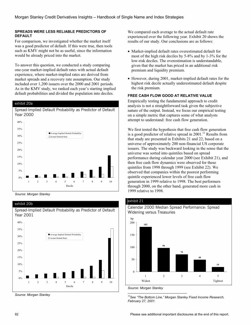
Morgan Stanley Credit Derivatives Insights – Handbook of Single Name and Index Strategies
92 Please see additional important disclosures at the end of this report.
SPREADS WERE LESS RELIABLE PREDICTORS OF DEFAULT For comparison, we investigated whether the market itself was a good predictor of default. If this were true, then tools such as KMV might not be as useful, since the information would be already priced into the market.
To answer this question, we conducted a study comparing one-year market-implied default rates with actual default experience, where market-implied rates are derived from market spreads and a recovery rate assumption. Our study included over 1,200 issuers over the 2000 and 2001 periods. As in the KMV study, we ranked each year’s starting implied default probabilities and divided the population into deciles.
exhibit 20a
Spread-Implied Default Probability as Predictor of Default Year 2000
0%
5%
10%
15%
20%
25%
30%
35%
40%
1 2 3 4 5 6 7 8 9 10Decile
Average Implied Default ProbabilityActual Default Rate
Source: Morgan Stanley
exhibit 20b
Spread-Implied Default Probability as Predictor of Default Year 2001
0%
5%
10%
15%
20%
25%
30%
35%
40%
1 2 3 4 5 6 7 8 9 10Decile
Average Implied Default Probability
Actual Default Rate
Source: Morgan Stanley
We compared each average to the actual default rate experienced over the following year. Exhibit 20 shows the results of our study. Our conclusions are as follows:
• Market-implied default rates overestimated default for most of the high risk deciles by 5-8% and by 1-3% for the low-risk deciles. The overestimation is understandable, given that the market has priced in an additional risk premium and liquidity premium.
• However, during 2001, market-implied default rates for the highest risk decile actually underestimated default despite the risk premium.
FREE CASH FLOW GOOD AT RELATIVE VALUE Empirically testing the fundamental approach to credit analysis is not a straightforward task given the subjective nature of the output. Instead, we focus our empirical testing on a simple metric that captures some of what analysts attempt to understand: free cash flow generation.
We first tested the hypothesis that free cash flow generation is a good predictor of relative spread in 2001.12 Results from that study are presented in Exhibits 21 and 22, based on a universe of approximately 200 non-financial US corporate issuers. The study was backward looking in the sense that the universe was sorted into quintiles based on spread performance during calendar year 2000 (see Exhibit 21), and then free cash flow dynamics were observed for these quintiles from 1998 through 1999 (see Exhibit 22). We observed that companies within the poorest performing quintile experienced lower levels of free cash flow generation in 1999 relative to 1998. The best performers through 2000, on the other hand, generated more cash in 1999 relative to 1998.
exhibit 21
Calendar 2000 Median Spread Performance: Spread Widening versus Treasuries
182
96
48
19
70
0
50
100
150
200
1 2 3 4 5Widest Tightest
bp
Source: Morgan Stanley 12See “The Bottom Line,” Morgan Stanley Fixed Income Research, February 27, 2001.

Section B, Chapter 13 Valuing Corporate Credit: Quantitative Approaches vs. Fundamental Analysis
Please see additional important disclosures at the end of this report. 93
exhibit 22
Median Free Cash Flow/Debt Changes: 1998 versus 1999
-3.3%
1.1%0.4%
5.0%
2.2%
-6%
-4%
-2%
0%
2%
4%
6%
1 2 3 4 5Widest Tightest
Source: Morgan Stanley
Exhibit 23 shows median spread performance versus free cash flow trends for the major sectors. Again, prior free cash flow trends are reasonably descriptive of subsequent performance.
exhibit 23
Sector 1998-1999 Free Cash Flow and 2000 Spread Performance
Utilities
Retail
RailsPipes
PhonesMedia
LeisureHealth
EnergyConsumer
Basic
Autos
Airlines
Aero
R2 = 0.1049
-100
-50
0
50
100
150
-15.0% -10.0% -5.0% 0.0% 5.0% 10.0% 15.0% 20.0%
Avg Change in FCF/Debt 1998-1999
2000 Spread Perf. Rel. to Mkt. (bp)
Source: Morgan Stanley
We conducted a similar study for European issuers more recently (spread changes in 2001 based on free cash flow dynamics from 1999 to 2000). In Exhibit 24 we show the free cash flow sector relationships based on a universe of the top 50 non-financial European corporate bond issuers, which account for about 70-80% of all European corporate debt outstanding. Again, we believe that free cash flow generation was a good predictor of spread change.
exhibit 24
Sector 1999-2000 Free Cash Flow Changes versus 2001 Spread Performance
-10
0
10
20
30
40
50
-4,000 -3,000 -2,000 -1,000 0 1,000 2,000 3,000
Sector FCF Change 1999-2000, € mm
2001 Spread Perf.Rel. to Mkt. (bp)
Autos
Industrials
Consumer Staples
Telecoms
Utilities
Source: Morgan Stanley
RATINGS ARE CONSISTENT WITH HISTORICAL EXPERIENCE Ratings agencies have been criticized for being both too slow and too quick in their ratings decisions. The agencies, for their part, consider it their job to produce ratings that, over time, match a default rate (expected loss), which in turn is based on historical experience. Hence, when judging the performance of the agencies, one needs to focus on the historical relationship between ratings and default rates.
Exhibit 26 shows average cumulative default rates by rating using Moody’s historical data from 1970-2001. The data show a strong correlation between ratings and default rates. Over a five-year horizon, for instance, the cumulative default rate of Baa-rated companies is almost 14 times that of Aaa-rated companies. Similarly, the cumulative default rate of speculative grade companies is almost 23 times that of investment grade companies.

Morgan Stanley Credit Derivatives Insights – Handbook of Single Name and Index Strategies
94 Please see additional important disclosures at the end of this report.
Exhibit 25 illustrates the relationship between ratings outlooks and subsequent defaults. Speculative-grade issuers with negative outlooks are, on average, nearly five times more likely to default than those with positive outlooks. The multiple is highest for the one-year default rate, in which companies with negative outlooks are over nine times more likely to default.
exhibit 25
S&P Average Cumulative Default Rates (1987-2000) Outlook Rating Year 1 (%) Year 2 (%) Year 3 (%)Stable AAA 0.00 0.00 0.00Negative AAA 0.00 0.00 0.00Positive AA 0.00 0.00 0.00Stable AA 0.00 0.03 0.07Negative AA 0.10 0.22 0.35Positive A 0.00 0.00 0.00Stable A 0.03 0.05 0.07Negative A 0.07 0.21 0.29Positive BBB 0.10 0.33 0.33Stable BBB 0.15 0.20 0.39Negative BBB 0.19 0.52 1.04Positive BB 0.12 1.30 2.35Stable BB 0.34 1.72 3.59Negative BB 2.64 6.86 10.44Positive B 2.42 7.55 12.63Stable B 2.76 8.45 12.80Negative B 9.65 18.05 23.72Positive CCC 2.08 2.08 6.25Stable CCC 7.84 15.16 20.42Negative CCC 29.18 37.95 44.53
Source: S&P
ConclusionClearly the topics we have discussed in this chapter are individually worthy of much more in-depth research. Our purpose in juxtaposing them in this chapter is to help investors gain insight into valuing corporate credit and select the most appropriate approach, or combinations of approaches, for a given situation. As we alluded to in our introduction to this chapter, these approaches each have their benefits and drawbacks, and we recommend that investors think about a given company along the three dimensions noted earlier to help decide which approach is best:
• Distance to default
• Leverage, or the ability to service debt from operations
• The management option to change the capital structure
Another issue which can dictate the usefulness of the various approaches is investor profile. In particular, it is important to distinguish those investors who are sensitive to mark-to-market fluctuations from those who are focused on absolute return to maturity. The latter may find the long-term signals provided by credit analysts, rating agencies, and quantitative models to be more important than the near-term risks priced into the market.
Finally, it is important to understand that credit investors, traders, and analysts do not have to select a single approach to value corporate credit as combinations of approaches may prove to be particularly insightful. For example, credit analysts could find structural models very useful in measuring the sensitivity of company valuations to changes in balance sheet items and cash flow projections. Similarly, investors and traders may combine analysts’ projections for a company with structural models to understand the potential impact corporate actions could have on valuation. In conclusion, rather than idealistically selecting a single approach, we encourage market participants to understand all approaches and select the best method or combinations of methods for a given investment situation.
exhibit 26
Moody’s Average Cumulative Default Rates by Letter Rating, 1970-2001 1 2 3 4 5 6 7 8 9 10 11 12 13 14 15 16 17 18 19 20Aaa - - - 0.04 0.14 0.25 0.37 0.49 0.64 0.79 0.96 1.15 1.36 1.48 1.60 1.74 1.88 2.03 2.03 2.03Aa 0.02 0.04 0.08 0.20 0.31 0.44 0.56 0.69 0.79 0.89 1.01 1.18 1.37 1.64 1.76 1.90 2.13 2.31 2.62 2.87A 0.02 0.07 0.21 0.35 0.51 0.68 0.87 1.07 1.32 1.57 1.84 2.09 2.38 2.62 2.97 3.35 3.78 4.30 4.88 5.44Baa 0.15 0.46 0.97 1.44 1.95 2.54 3.16 3.75 4.40 5.09 5.85 6.64 7.42 8.23 9.10 9.94 10.76 11.48 12.05 12.47Ba 1.27 3.57 6.20 8.83 11.42 13.75 15.63 17.58 19.46 21.27 23.23 25.36 27.38 29.14 30.75 32.62 34.24 35.68 36.88 37.97B 6.66 13.99 20.51 26.01 31.00 35.15 39.11 42.14 44.80 47.60 49.65 51.23 52.91 54.70 55.95 56.73 57.20 57.20 57.20 57.20Caa-C 21.99 34.69 44.43 51.85 56.82 62.07 66.61 71.18 74.64 77.31 80.55 80.55 80.55 80.55 80.55 80.55 80.55 80.55 80.55 80.55Investment Grade 0.06 0.19 0.38 0.65 0.90 1.19 1.50 1.81 2.15 2.15 2.51 2.89 3.30 3.72 4.15 4.60 5.08 5.58 6.55 6.96Speculative Grade 4.73 9.55 13.88 17.62 20.98 23.84 26.25 28.42 30.40 32.31 34.19 36.05 37.83 39.44 40.84 42.37 43.67 44.78 45.71 46.58All Corps 1.54 3.08 4.46 5.65 6.67 7.57 8.34 9.04 9.71 10.37 11.03 11.70 12.36 12.98 13.58 14.22 14.84 15.42 15.96 16.43
Source: Moody’s

Please see additional important disclosures at the end of this report. 95
Chapter 14
Libor Metrics June 27, 2003
Primary Analyst: Sivan Mahadevan Primary Analyst: Peter Polanskyj Primary Analyst: Rizwan Hussain Anisha Ambardar
A combination of low spreads, high dollar prices and a steep yield curve has made relative value analyses difficult today, both within the universe of corporate bonds and between bonds and default swaps. Looking at bonds on a Libor basis is supposed to be the common denominator approach, but confusion persists. Using Libor spreads is a bit like the Metric System: everyone agrees that it is better, but it is hard to develop intuition for the measures when the market trades on Treasury spread and dollar price.
We focus on describing the various Libor spread measures in simple terms, recommend using the intuitive Z-Spread approach for relative value purposes (for both cash investors and derivatives users), and show some practical examples to illustrate relative value in an environment where a handful of basis points really matter.
FOUR LIBOR MEASURES Four Libor spread measures are commonly used by market participants. Par and market value asset swaps are meant to be used by those doing real asset swaps (i.e., converting a fixed rate bond to a floating rate instrument), while interpolated swap curve spreads and Z-Spreads are relative value measures used by those who are focusing on fixed rate assets.
exhibit 1
Par Asset Swap – 8% 10-Year Bond Priced at $110
0 3 6 120Months
110
4
F F F
4
10
4
104
Investor
Bond
Swap Counterparty
Notional Amount = 100
Note: The floating payment F equals Notional Amount*(LIBOR + Spread) / 4.
Source: Morgan Stanley
ASSET SWAPS A par asset swap is the most common type of fixed for floating swap used by credit investors. If a bond trades at par, then the swap simply involves an exchange of coupon payments for
floating rate Libor plus a fixed spread. When a bond trades at a premium, the swap becomes off-market, and there is typically an upfront payment from the swap counterparty to the investor to make up for the premium (see Exhibit 1).
A market value asset swap is less common and involves converting the fixed-rate bond into a floating rate note with par equal to the original bond’s dollar price.
MAKING UP FOR UNACCOUNTED CREDIT RISK While asset swaps are practical vehicles for converting fixed-rate bonds to floating rate, the “spread” over Libor paid out by the swap counterparty is not necessarily an accurate measure of the credit risk of the bond. This is even truer when there are upfront or residual payments.
In a par asset swap, the present value of all the periodic cash flows is equal to the premium or discount on the bond. This present value is calculated using the Libor term structure, while the premium on the bond is a result of cash flows, which are discounted using a credit-risky rate. As a result, asset swap spreads reflect the shape of the Libor yield curve but fail to fully incorporate the impact of the credit-risky nature of the bond cash flows. This mismatch in discount rates introduces a bias in the asset swap spreads, which is particularly acute for bonds with significant premiums or discounts, as well as bonds with wide credit spreads.
One point we want to make clear is that asset swaps are not incorrectly measuring credit risk. Indeed, the swap itself has no credit exposure (to the bond issuer) because all of the payments on the swap are due whether or not the bond defaults prior to maturity.
GOING BACK TO BASICS For investors who are simply using Libor measures to make relative value decisions between bonds and/or default swaps, we consider two other measures more relevant. Both measures involve a common and intuitive practice, namely comparing a bond’s yield or cash flows to a benchmark. An interpolated swap spread is one measure and is simply the yield to maturity of a bond minus the interpolated yield on the swap curve. This spread is termed I-Spread (or yield-on-yield spread by asset swappers).
I-Spread ignores the shape of both the Libor yield curve and the credit curve, and thus does not reflect any impact for the actual timing of payments. Two bonds with the same maturity and yield but different coupons (and thus different duration) would get the same I-Spread.
The second solution is to take a step back and think about bond basics. What investors require is a method to compare a
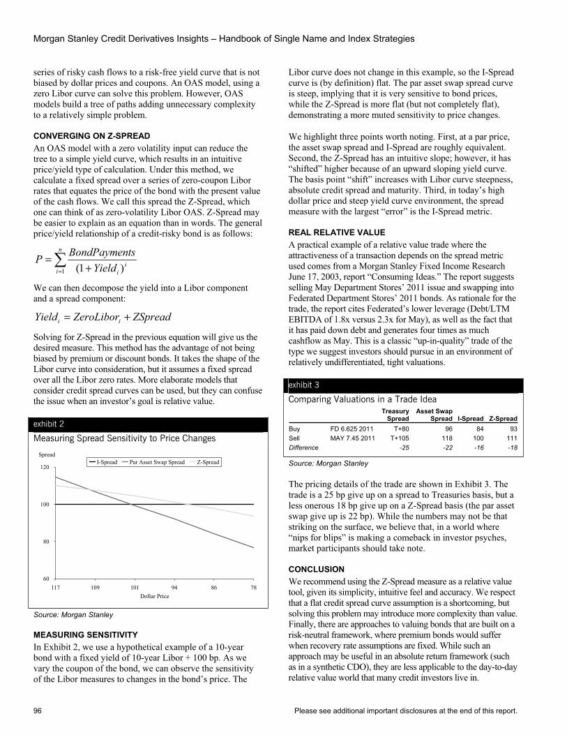
Morgan Stanley Credit Derivatives Insights – Handbook of Single Name and Index Strategies
96 Please see additional important disclosures at the end of this report.
series of risky cash flows to a risk-free yield curve that is not biased by dollar prices and coupons. An OAS model, using a zero Libor curve can solve this problem. However, OAS models build a tree of paths adding unnecessary complexity to a relatively simple problem.
CONVERGING ON Z-SPREAD An OAS model with a zero volatility input can reduce the tree to a simple yield curve, which results in an intuitive price/yield type of calculation. Under this method, we calculate a fixed spread over a series of zero-coupon Libor rates that equates the price of the bond with the present value of the cash flows. We call this spread the Z-Spread, which one can think of as zero-volatility Libor OAS. Z-Spread may be easier to explain as an equation than in words. The general price/yield relationship of a credit-risky bond is as follows:
= +=
n
ii
iYieldtsBondPaymenP
1 )1(
We can then decompose the yield into a Libor component and a spread component:
ZSpreadZeroLiborYield ii +=
Solving for Z-Spread in the previous equation will give us the desired measure. This method has the advantage of not being biased by premium or discount bonds. It takes the shape of the Libor curve into consideration, but it assumes a fixed spread over all the Libor zero rates. More elaborate models that consider credit spread curves can be used, but they can confuse the issue when an investor’s goal is relative value.
exhibit 2
Measuring Spread Sensitivity to Price Changes
Spread
60
80
100
120
117 109 101 94 86 78Dollar Price
I-Spread Par Asset Swap Spread Z-Spread
Source: Morgan Stanley
MEASURING SENSITIVITY In Exhibit 2, we use a hypothetical example of a 10-year bond with a fixed yield of 10-year Libor + 100 bp. As we vary the coupon of the bond, we can observe the sensitivity of the Libor measures to changes in the bond’s price. The
Libor curve does not change in this example, so the I-Spread curve is (by definition) flat. The par asset swap spread curve is steep, implying that it is very sensitive to bond prices, while the Z-Spread is more flat (but not completely flat), demonstrating a more muted sensitivity to price changes.
We highlight three points worth noting. First, at a par price, the asset swap spread and I-Spread are roughly equivalent. Second, the Z-Spread has an intuitive slope; however, it has “shifted” higher because of an upward sloping yield curve. The basis point “shift” increases with Libor curve steepness, absolute credit spread and maturity. Third, in today’s high dollar price and steep yield curve environment, the spread measure with the largest “error” is the I-Spread metric.
REAL RELATIVE VALUE A practical example of a relative value trade where the attractiveness of a transaction depends on the spread metric used comes from a Morgan Stanley Fixed Income Research June 17, 2003, report “Consuming Ideas.” The report suggests selling May Department Stores’ 2011 issue and swapping into Federated Department Stores’ 2011 bonds. As rationale for the trade, the report cites Federated’s lower leverage (Debt/LTM EBITDA of 1.8x versus 2.3x for May), as well as the fact that it has paid down debt and generates four times as much cashflow as May. This is a classic “up-in-quality” trade of the type we suggest investors should pursue in an environment of relatively undifferentiated, tight valuations.
exhibit 3
Comparing Valuations in a Trade Idea Treasury
SpreadAsset Swap
Spread I-Spread Z-SpreadBuy FD 6.625 2011 T+80 96 84 93Sell MAY 7.45 2011 T+105 118 100 111Difference -25 -22 -16 -18
Source: Morgan Stanley
The pricing details of the trade are shown in Exhibit 3. The trade is a 25 bp give up on a spread to Treasuries basis, but a less onerous 18 bp give up on a Z-Spread basis (the par asset swap give up is 22 bp). While the numbers may not be that striking on the surface, we believe that, in a world where “nips for blips” is making a comeback in investor psyches, market participants should take note.
CONCLUSIONWe recommend using the Z-Spread measure as a relative value tool, given its simplicity, intuitive feel and accuracy. We respect that a flat credit spread curve assumption is a shortcoming, but solving this problem may introduce more complexity than value. Finally, there are approaches to valuing bonds that are built on a risk-neutral framework, where premium bonds would suffer when recovery rate assumptions are fixed. While such an approach may be useful in an absolute return framework (such as in a synthetic CDO), they are less applicable to the day-to-day relative value world that many credit investors live in.

Please see additional important disclosures at the end of this report. 97
Chapter 15
A Tale of Two Credit Markets August 8, 2003
Primary Analyst: Sivan Mahadevan Primary Analyst: Peter Polanskyj Anisha Ambardar
We have an interesting story to tell. It may be not as literary as those of Charles Dickens, but it is certainly relevant to credit investors wondering what happened to corporate credit with all of the swap spread dynamics over the past several trading days. In a nutshell, the gigantic move in interest rates forced mortgage investors to hedge, which blew out swap spreads by 20-30 bp. Initially, corporate credit markets did not react, leaving many “spread over Libor” advocates kind of puzzled. Eventually credit markets moved (and maybe by too much), but the correction was forced by derivatives users, who were able to capitalize on the “dislocation.” Spreads over Treasuries are now even wider than they were before the swap spread episode, leaving the ball in the “real money” court.
Market participants learned quite a bit during this process, and we argue that it is important to put this down in writing so that we don’t forget (or get caught on the wrong side) the next time it happens.
IT WAS THE WORST OF TIMES Everyone knows that mortgage-backed securities are prepayment sensitive instruments that are negatively convex and effectively “short” an option that is influenced by the level and volatility of Treasury rates. The historically significant move in Treasury rates over the past three weeks put this phenomenon in the spotlight and forced mortgage investors (and the agencies) to chase the market to readjust duration and battle the negative convexity of their instruments. As a result, swap spreads blew out by 20-30 bp, based purely on flows from these institutions.
IMMEDIATE REACTION: A TIME OF WISDOM OR FOOLISHNESS?Credit instruments that are “linked” directly to Libor (floating rate paper, ABS and even agencies) became instantly cheaper versus Treasuries as swap spreads blew out, even though perceived “credit” risk in the financial markets did not really change. This cheapness occurred while fixed-rate corporate bonds remained stable on a Treasury spread basis and thus became rich to Libor. Credit default swaps did not move much, driving the basis (CDS minus cash bond Libor spread) significantly wider, into positive territory.
Flows in mortgages and other Libor products have subsequently driven swap spreads back down. This swap spread boomerang suggests that the recent swap spread widening was based on technical factors rather than fundamental changes in perceived risk.
THIS TIME IT WAS DIFFERENT Turning the clock back, we note that many sharp moves in swap spreads were accompanied by severe moves in corporate credit spreads as well, generally without much of a lead or lag (see Exhibit 1). During those periods, corporate credit risk increased, and arguably the same fear that drove corporate spreads wider influenced swaps spreads as well.
exhibit 1
Strong Links in Times of Crisis bp
0
50
100
150
200
250
300
Jul-95 Mar-97 Oct-98 May-00 Dec-01 Aug-03
5 Year Swap Spread Investment Grade Credit
Russia / LTCM Crisis
End of Equity Bull Market
Corporate Governance Crisis
Source: Bloomberg, Salomon Analytics
Yet, the recent market activity is telling us that it was different this time. When swap spreads began moving wider (July 28, 2003), corporate bonds did not react. Effectively, corporates “rallied” versus swaps. If we were in a new swap spread regime, the rational trade would be to sell corporates outright or at least in favor of credit instruments that are “linked” to Libor. The idea behind this trade is that corporates would eventually catch up. “Real money” did not do this trade because, in our view, they did not feel that the swap spread move reflected increased systemic risk. It was hard to let go of those bonds based solely on a technicality, albeit a strong one.
This lack of action by corporate bond investors spurred a lot of discussion. Mortgage, agency and ABS investors wondered why corporates “still trade to Treasuries” while corporate investors wondered why they should care.
ENTER THE CREDIT DERIVATIVES MARKET: THE SPRING OF HOPE Many credit derivatives users have been positioned in a “negative basis” trade. With bonds trading wider than default swaps, the trade of buying a bond and buying protection was a
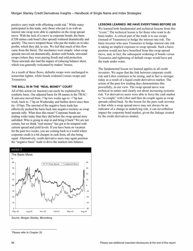
Morgan Stanley Credit Derivatives Insights – Handbook of Single Name and Index Strategies
98 Please see additional important disclosures at the end of this report.
positive carry trade with offsetting credit risk.1 While many participated in this trade, only those who put it on with an interest rate swap were able to capitalize on the swap spread move. With the lack of a move in corporate bonds, the basis (CDS minus cash bond Libor spread) widened dramatically and quickly. This move tempted those who put the trades on to take profits, which they did, in size. We feel that much of this flow came from the Street. The mechanics were simple: when swap spreads moved out dramatically, dealers sold bonds, unwound swaps (where they were paying fixed) and sold protection. These unwinds also had the impact of reducing balance sheet, which was generally welcomed by traders’ bosses.
As a result of these flows, defaults swaps were unchanged to somewhat tighter, while bonds widened (versus swaps and Treasuries).
THE BALL IS IN THE “REAL MONEY” COURT All of this action (or inaction) can easily be explained by the synthetic basis. Our adjusted basis for 88 names in the TRAC-X universe moved from -7 bp two weeks ago to +7 bp last week, back to -7 bp on Wednesday and further down since then (to -10 bp). The unwind of the negative basis trade has effectively pushed the basis back into negative territory as swap spreads rally. What does this mean? Corporate bonds are trading wider today than they did before the swap spread story unfolded. Who is going to step in and bring it back? We are not certain, but we think “real-money” has got to be tempted with current spread and yield levels. If you have been on vacation for the past two weeks, you are coming back to a world where corporate credit is a bit cheaper in cash form, all else being equal. Alternatively, credit derivative users may again position the “negative basis” trade to drive the markets into balance.
exhibit 2
The Basis Move bp
0
10
20
30
40
50
60
70
80
May-02 Aug-02 Nov-02 Feb-03 May-03 Aug-03-40
-30
-20
-10
0
10
20
30
405Y Swap Spread Unadjusted Basis
Source: Morgan Stanley, Bloomberg
1Please refer to Chapter 35.
LESSONS LEARNED: WE HAVE EVERYTHING BEFORE US We learned both fundamental and technical lessons from this “event.” The technical lesson is for those who want to do basis trades. A critical part of the trade is to use swaps (instead of Treasuries) to hedge the interest rate risk. The basis investor who uses Treasuries to hedge interest rate risk is taking an implicit exposure to swap spreads. Such a basis position would not have benefited from this swap spread move, and, in fact, the subsequent widening of bonds versus Treasuries and tightening of default swaps would have put the trade under water.
The fundamental lesson we learned applies to all credit investors. We argue that the link between corporate credit risk and Libor continues to be strong, and in fact is stronger today as a result of a liquid credit derivatives market. The action of the past few trading days demonstrates this powerfully, in our view. The swap spread move was technical in nature and clearly not about increasing systemic risk. Yet derivatives users were able to force the cash market to “re-couple” with Libor and then de-couple again as swap spreads rallied back. So the lesson for the pure cash investor is that while a swap spread move may not always be an indicator of a change in underlying risk, it can nevertheless impact the corporate bond market, given the linkage created by the credit derivatives market.

Please see additional important disclosures at the end of this report. 99
Chapter 16
Making a Point – Upfront September 19, 2003
Primary Analyst: Sivan Mahadevan Primary Analyst: Peter Polanskyj Anisha Ambardar
A year ago, single-name credit derivatives were in the spotlight, given the high levels of credit volatility, idiosyncratic risk and hedging activity. Market participants focused on flows and liquidity, and, when they could, thought about things like the value of restructuring and expected ISDA definitions. Today, with markets much quieter, we argue for more of a relative value play, and we encourage investors to brush up on the details, as doing so may define fourth quarter and 2004 opportunities.
We have addressed bond versus default swap trading strategies in previous research,1 but one detail that continues to draw questions is the motivation and mechanics behind credits trading with “points upfront.” We focus on this concept in a relative value framework, considering American Airlines unsecured protection the relevant example.
THE MECHANICS OF TRADING UPFRONT When a credit is distressed, it often trades with points upfront. Dealers quote the CDS with a fixed premium (say 500 bp running) and then adjust for bid-offer and market movements with a points upfront quote. For example, American Airlines (AMR) unsecured protection to September 2013 currently trades at 39/44 points upfront plus 500 bp running (with no restructuring). The buyer of protection will pay 44% of notional upfront, and then pay 500 bp per annum until the protection maturity date, if there is no credit event to terminate the swap. The seller of protection receives 39 points upfront and 500 bp running. Why do credits trade with points upfront, and when does the market decide to change quoting conventions?
MOTIVATION FOR TRADING UPFRONT – ARBITRAGE FORCES The motivation and details behind a credit trading upfront has everything to do with arbitrage forces. A trader who bids protection on AMR may look for a cash bond to use as a hedge for the protection. The fixed rate bond “plus” the protection results in a default-risk free position; thus, the numbers need to add up, otherwise an arbitrage opportunity arises.
If we consider the AMR 9% of 2012 as a reference bond, the terms of the AMR protection begin to make sense. Given the protection pricing (the points upfront curve is flat from 2008 through 2013), if a trader can purchase the AMR bond for a hypothetical price of $61 (it doesn’t actually trade there – see below), then he or she has built a default-risk free position, more or less (see Exhibit 1). The combined bond and
1Please refer to Section C.
protection position results in an annual coupon stream of 4% (9% minus 5%), which is approximately equal to 10-year Libor. A 10-year credit-risk free instrument with fixed coupons equal to 10-year Libor should have a price near par, which is what the trader has effectively paid ($61 for the bond plus 39 points upfront for the protection).
In theory, this market behavior should be true for any credit trading away from par, but in practice, market makers only demand upfront payments when there is a significant deviation, as that is when carry and the timing of cash flows begin to really matter. Clearly, they matter even more if the credit has a high probability of default.
exhibit 1
AMR Bonds and Protection – Back of the Envelope Arbitrage Relation
Instrument Maturity Price/Points
Upfront CouponPrincipal Payment
Buy Protection 2012 (39) (5%) 0Buy AMR 9% 2012 2012 (Implied = 61)* 9% 100Net Position 2012 (100) 4% 100
Note: Arbitrage relationship implies a $61 price for the AMR bond. Source: Morgan Stanley
DISCOUNT BONDS AND DEFAULT EXPOSURE From Exhibit 1 we can see that selling protection with an upfront fee has the same economics as buying a bond at a discount. This risk profile is similar to a par bond with a coupon roughly equal to swaps + 2100 bp. Yet this coupon is not certain and the seller of protection therefore has a different default exposure than the seller who gets paid upfront. The exposure for the par CDS is nominally greater, initially, but it converges with the upfront trade over time (see Exhibit 2). While it is clear that the seller of protection on
exhibit 2
Less Near-Term Default Exposure: Upfront vs. Par CDS
2003 2004 2005 2006 2007 2008 2009 2010 2011 2012 2013
Upfront CDSPar CDS
50%
55%
60%
65%
70%
75%
80%
85%
90%
95%
100%
Calendar Year
Upfront CDSPar CDS
Source: Morgan Stanley
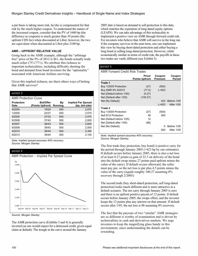
Morgan Stanley Credit Derivatives Insights – Handbook of Single Name and Index Strategies
100 Please see additional important disclosures at the end of this report.
a par basis is taking more risk, he/she is compensated for that risk by the much higher coupon. To understand the nature of the increased coupon, consider that the PV of 1600 bp (the difference in coupons) is much greater than 39 points (the upfront CDS fee) when discounted at Libor; however, the two are equivalent when discounted at Libor plus 2100 bp.
AMR – UPFRONT RELATIVE VALUE Going back to the AMR example, although the “arbitrage free” price of the 9% of 2012 is $61, the bonds actually trade much richer (75½/77½). We attribute this richness to important technicalities, including difficulty shorting the bond and demand from bond investors for the “optionality” associated with American Airlines surviving.
Given this implied richness, are there others ways of betting that AMR survives?
exhibit 3
AMR Protection Curve Protection Date
Bid/Offer (Points Upfront)
BpRunning
Implied Par Spread (bp, bid side)
9/2004 19/24 500 2,8751/2005 22/27 500 2,5759/2005 27/32 500 2,5759/2006 37/42 500 2,8009/2007 38/43 500 2,6009/2008 39/43 500 2,5009/2010 39/44 500 2,3009/2013 39/44 500 2,100
Note: Implied spread assumes 40% recovery. Source: Morgan Stanley
exhibit 4
AMR Protection – Implied Par Spread Curve
bp
2,000
2,200
2,400
2,600
2,800
3,000
Sep-04 Sep-05 Sep-06 Sep-07 Sep-08 Sep-09 Sep-10 Sep-11 Sep-12 Sep-13
Source: Morgan Stanley
The AMR protection curve (Exhibits 3 and 4) is generally inverted (as one would expect for a distressed credit, given equal claim at default). The trough in the curve around the January
2005 date is based on demand to sell protection to this date, which matches the expiration of long-dated equity options (LEAPS). We can take advantage of this technicality to implement a positive view on AMR through forward credit risk. For investors who believe that AMR will survive in the long run if the company survives in the near-term, one can implement this view by buying short-dated protection and either buying a long bond or selling long-dated protection. However, while economically similar in terms of credit risk, the payoffs in these two trades are vastly different (see Exhibit 5).
exhibit 5
AMR Forward Credit Risk Trades Price/
Points Upfront Coupon/Premium
CouponPeriod
Trade 1 Buy 1/2005 Protection (27) (500)Buy AMR 9% 8/2012 (77.5) L+923Net (Default before 1/05) (0.27)Net (Default after 1/05) (100.27) Net (No Default) 423
L+923Before 1/05
After 1/05Trade 2 Buy 1/2005 Protection (27) (500)Sell 9/12 Protection 39 500Net (Default before 1/05) 12 Net (Default after 1/05) (88) Net (No Default) 0
500Before 1/05
After 1/05
Note: Implied spread assumes 40% recovery. Source: Morgan Stanley
The first trade (buy protection, buy bond) is positive carry for the period through January 2005 (+423 bp by our estimates). If default occurs before January 2005, there is also a net loss of at least 0.27 points (a gain of 22.5 on delivery of the bond into the default swap minus 27 points paid upfront minus the value of the carry). If default occurs afterward, the seller must pay par, so the net loss is par plus 4.5 points minus the value of the carry (equals roughly 100.27 assuming 0% recovery through 2/2005).
The second trade (buy short-dated protection, sell long-dated protection) looks much different and is more attractive in a default scenario. The net carry through January 2005 is zero and there is an upfront positive payout of 12 points. If default occurs before January 2005, the swaps offset, and the investor keeps the 12 points plus any interest on that amount. If default occurs after 1/05, the net loss is 88 assuming 0% recovery.
The fact that the payouts of two “similar” AMR strategies are so different is worthy of examination and is driven by technicalities in cash and derivatives markets. We urge investors to keep the magnifying glass handy in this environment, since understanding the details can be rewarding.
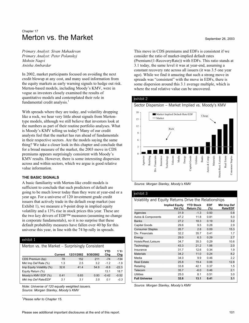
Please see additional important disclosures at the end of this report. 101
Chapter 17
Merton vs. the Market September 26, 2003
Primary Analyst: Sivan Mahadevan Primary Analyst: Peter Polanskyj Mohsin Naqvi Anisha Ambardar
In 2002, market participants focused on avoiding the next credit blowup at any cost, and many used information from the equity markets as early warning signals to hedge out risk. Merton-based models, including Moody’s KMV, were in vogue as investors closely examined the results of quantitative models and contemplated their role in fundamental credit analysis.1
With spreads where they are today, and volatility dropping like a rock, we hear very little about signals from Merton-type models, although we still believe that investors look at the numbers as part of their routine portfolio analyses. What is Moody’s KMV telling us today? Many of our credit analysts feel that the market has run ahead of fundamentals in their respective sectors. Are the models saying the same thing? We take a closer look in this chapter and conclude that for a broad measure of the market, the 2003 move in CDS premiums appears surprisingly consistent with Moody’s KMV results. However, there is some interesting dispersion across and within sectors, which we argue is good relative value information.
THE BASIC SIGNALS A basic familiarity with Merton-like credit models is sufficient to conclude that such predictors of default are going to be much lower today than they were at year-end or a year ago. For a universe of 120 investment grade credit issuers that actively trade in the default swap market (see Exhibit 1), we measure a 9-point drop in implied equity volatility and a 13% rise in stock prices this year. These are the two key drivers of EDF™ measures (assuming no change in corporate fundamentals), so it is no surprise that these default probability measures have fallen over 40 bp for this universe this year, in line with the 74 bp rally in spreads.
exhibit 1
Merton vs. the Market – Surprisingly Consistent
Current 12/31/2002 9/30/2002 YTDChg
1 Yr Chg
CDS Premium (bp) 78 152 211 -74 -134Mkt Imp Def Rate (%) 1.3 2.5 3.2 -1.2 -1.9Imp Equity Volatility (%) 32.6 41.4 54.9 -8.8 -22.3Equity Return (%) 13.1 18.7Moody’s KMV EDF (%) 0.41 0.83 0.93 -0.42 -0.52Mkt Imp Def Rate/EDF 3.1 3.1 3.5 0.1 -0.3
Note: Universe of 120 equally weighted issuers. Source: Morgan Stanley, Moody’s KMV 1Please refer to Chapter 15.
This move in CDS premiums and EDFs is consistent if we consider the ratio of market-implied default rates (Premium/(1-RecoveryRate)) with EDFs. This ratio stands at 3.1 today, the same level it was at year-end, assuming a constant recovery rate across all issuers (it was 3.5 one year ago). While we find it amazing that such a strong move in spreads was “consistent” with the move in EDFs, there is some dispersion around this 3.1 average multiple, which is where the real relative value can be uncovered.
exhibit 2
Sector Dispersion – Market Implied vs. Moody’s KMV
0
3
6
9
12
15
18
Age
ncie
s
Ret
ailin
g
Div
. Fin
anci
als
Insu
ranc
e
Tech
nolo
gy
Tele
com
Med
ia
Ener
gy
Cap
ital G
oods
Util
ities
Ban
ks
Aut
os &
Com
p.
Mat
eria
ls
Hot
els/
Res
t./Le
isur
e
Rea
l Est
ate
Con
sum
er S
tapl
es
Market Implied Default Rate/EDFMarket
Rich
Cheap
Source: Morgan Stanley, Moody’s KMV
exhibit 3
Volatility and Equity Returns Drive the Relationships Implied Equity
Vol (%) YTD Stock Return (%)
EDF(%)
Mkt Imp Def Rate/EDF
Agencies 31.9 -1.3 0.50 0.8Autos & Components 47.2 11.8 0.81 5.0Banks 27.2 18.3 0.19 3.2Capital Goods 29.6 9.5 0.28 2.9Consumer Staples 26.7 2.8 0.09 15.3Div. Financials 32.2 35.7 0.41 1.7Energy 29.0 6.3 0.29 2.7Hotels/Rest./Leisure 34.7 35.3 0.29 10.6Technology 43.3 21.2 1.06 2.0Insurance 31.7 12.6 0.34 1.9Materials 34.2 11.0 0.24 8.2Media 34.0 9.9 0.46 2.2Real Estate 25.8 19.4 0.06 12.8Retailing 33.8 42.1 0.37 1.5Telecom 35.7 -6.0 0.46 2.1Utilities 25.0 8.1 0.51 3.0Full Universe 32.6 13.1 0.41 3.1
Source: Morgan Stanley, Moody’s KMV
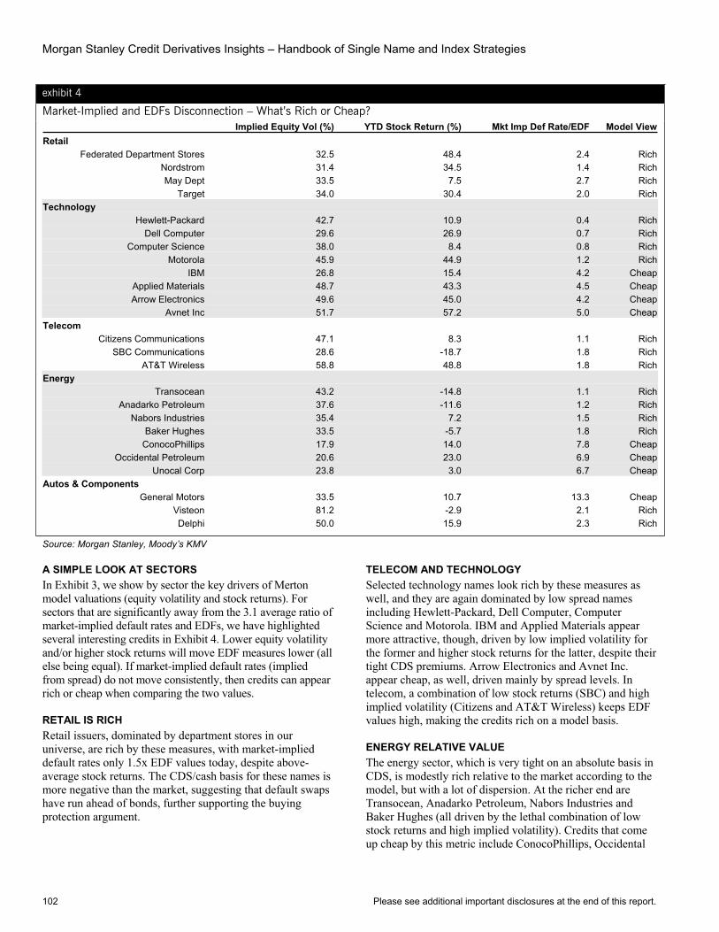
Morgan Stanley Credit Derivatives Insights – Handbook of Single Name and Index Strategies
102 Please see additional important disclosures at the end of this report.
exhibit 4
Market-Implied and EDFs Disconnection – What’s Rich or Cheap? Implied Equity Vol (%) YTD Stock Return (%) Mkt Imp Def Rate/EDF Model View
RetailFederated Department Stores 32.5 48.4 2.4 Rich
Nordstrom 31.4 34.5 1.4 RichMay Dept 33.5 7.5 2.7 Rich
Target 34.0 30.4 2.0 RichTechnology
Hewlett-Packard 42.7 10.9 0.4 RichDell Computer 29.6 26.9 0.7 Rich
Computer Science 38.0 8.4 0.8 RichMotorola 45.9 44.9 1.2 Rich
IBM 26.8 15.4 4.2 CheapApplied Materials 48.7 43.3 4.5 CheapArrow Electronics 49.6 45.0 4.2 Cheap
Avnet Inc 51.7 57.2 5.0 CheapTelecom
Citizens Communications 47.1 8.3 1.1 RichSBC Communications 28.6 -18.7 1.8 Rich
AT&T Wireless 58.8 48.8 1.8 RichEnergy
Transocean 43.2 -14.8 1.1 RichAnadarko Petroleum 37.6 -11.6 1.2 Rich
Nabors Industries 35.4 7.2 1.5 RichBaker Hughes 33.5 -5.7 1.8 Rich
ConocoPhillips 17.9 14.0 7.8 CheapOccidental Petroleum 20.6 23.0 6.9 Cheap
Unocal Corp 23.8 3.0 6.7 CheapAutos & Components
General Motors 33.5 10.7 13.3 CheapVisteon 81.2 -2.9 2.1 RichDelphi 50.0 15.9 2.3 Rich
Source: Morgan Stanley, Moody’s KMV
A SIMPLE LOOK AT SECTORS In Exhibit 3, we show by sector the key drivers of Merton model valuations (equity volatility and stock returns). For sectors that are significantly away from the 3.1 average ratio of market-implied default rates and EDFs, we have highlighted several interesting credits in Exhibit 4. Lower equity volatility and/or higher stock returns will move EDF measures lower (all else being equal). If market-implied default rates (implied from spread) do not move consistently, then credits can appear rich or cheap when comparing the two values.
RETAIL IS RICH Retail issuers, dominated by department stores in our universe, are rich by these measures, with market-implied default rates only 1.5x EDF values today, despite above-average stock returns. The CDS/cash basis for these names is more negative than the market, suggesting that default swaps have run ahead of bonds, further supporting the buying protection argument.
TELECOM AND TECHNOLOGY Selected technology names look rich by these measures as well, and they are again dominated by low spread names including Hewlett-Packard, Dell Computer, Computer Science and Motorola. IBM and Applied Materials appear more attractive, though, driven by low implied volatility for the former and higher stock returns for the latter, despite their tight CDS premiums. Arrow Electronics and Avnet Inc. appear cheap, as well, driven mainly by spread levels. In telecom, a combination of low stock returns (SBC) and high implied volatility (Citizens and AT&T Wireless) keeps EDF values high, making the credits rich on a model basis.
ENERGY RELATIVE VALUE The energy sector, which is very tight on an absolute basis in CDS, is modestly rich relative to the market according to the model, but with a lot of dispersion. At the richer end are Transocean, Anadarko Petroleum, Nabors Industries and Baker Hughes (all driven by the lethal combination of low stock returns and high implied volatility). Credits that come up cheap by this metric include ConocoPhillips, Occidental

Section B, Chapter 17 Merton vs. the Market
Please see additional important disclosures at the end of this report. 103
Petroleum and Unocal Corp, with low implied volatility being a key driver.
AUTOS AND CONSUMER STAPLES Ford and GM both look cheap on this model basis, which we attribute to wide spreads, combined with above-average equity performance for Ford and tame implied volatility for GM. The suppliers (Visteon and Delphi) come up rich, though, as significantly higher levels of implied volatility and stock underperformance drive EDF values higher. Consumer staples credits are surprisingly cheap per the model, but this is driven by incredibly low EDF values, which are in turn driven by a big drop off in implied equity volatility.
WHAT DOES ALL THIS MEAN? Many would argue that it is not easy to compare valuations from a risk-neutral world (where default risk is derived from
spreads) and the Merton (or structural) world. Yet we are doing so anyway because we believe investors need to synch-up the two worlds occasionally, as both approaches are used in the investment process. The Merton methodology is popular in the single-name world, but investors ultimately are motivated by spread, so we think the simple comparisons make for interesting relative value information.
There is an important disconnect between the single-name world and structured credit products (tranches and options), where risk-neutral approaches are employed to evaluate default risk. For the market at large, structured credit investors should be comforted by the consistency in the move in both worlds. However, the relative richness or cheapness of credits when cross comparisons are made should not go unnoticed by structured credit investors when making investment decisions.
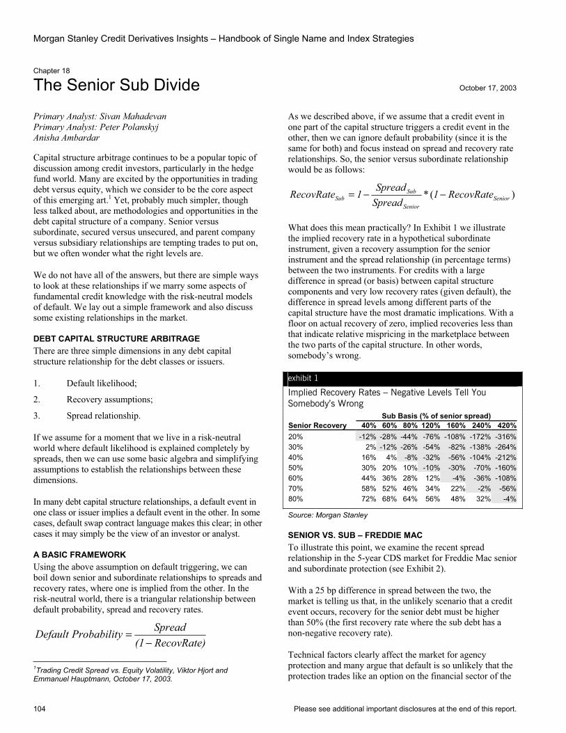
Morgan Stanley Credit Derivatives Insights – Handbook of Single Name and Index Strategies
104 Please see additional important disclosures at the end of this report.
Chapter 18
The Senior Sub Divide October 17, 2003
Primary Analyst: Sivan Mahadevan Primary Analyst: Peter Polanskyj Anisha Ambardar
Capital structure arbitrage continues to be a popular topic of discussion among credit investors, particularly in the hedge fund world. Many are excited by the opportunities in trading debt versus equity, which we consider to be the core aspect of this emerging art.1 Yet, probably much simpler, though less talked about, are methodologies and opportunities in the debt capital structure of a company. Senior versus subordinate, secured versus unsecured, and parent company versus subsidiary relationships are tempting trades to put on, but we often wonder what the right levels are.
We do not have all of the answers, but there are simple ways to look at these relationships if we marry some aspects of fundamental credit knowledge with the risk-neutral models of default. We lay out a simple framework and also discuss some existing relationships in the market.
DEBT CAPITAL STRUCTURE ARBITRAGE There are three simple dimensions in any debt capital structure relationship for the debt classes or issuers.
1. Default likelihood;
2. Recovery assumptions;
3. Spread relationship.
If we assume for a moment that we live in a risk-neutral world where default likelihood is explained completely by spreads, then we can use some basic algebra and simplifying assumptions to establish the relationships between these dimensions.
In many debt capital structure relationships, a default event in one class or issuer implies a default event in the other. In some cases, default swap contract language makes this clear; in other cases it may simply be the view of an investor or analyst.
A BASIC FRAMEWORK Using the above assumption on default triggering, we can boil down senior and subordinate relationships to spreads and recovery rates, where one is implied from the other. In the risk-neutral world, there is a triangular relationship between default probability, spread and recovery rates.
RecovRate)(1SpreadyProbabilitDefault
−=
1Trading Credit Spread vs. Equity Volatility, Viktor Hjort and Emmanuel Hauptmann, October 17, 2003.
As we described above, if we assume that a credit event in one part of the capital structure triggers a credit event in the other, then we can ignore default probability (since it is the same for both) and focus instead on spread and recovery rate relationships. So, the senior versus subordinate relationship would be as follows:
)(* SeniorSenior
SubSub RecovRate1
SpreadSpread
1RecovRate −−=
What does this mean practically? In Exhibit 1 we illustrate the implied recovery rate in a hypothetical subordinate instrument, given a recovery assumption for the senior instrument and the spread relationship (in percentage terms) between the two instruments. For credits with a large difference in spread (or basis) between capital structure components and very low recovery rates (given default), the difference in spread levels among different parts of the capital structure have the most dramatic implications. With a floor on actual recovery of zero, implied recoveries less than that indicate relative mispricing in the marketplace between the two parts of the capital structure. In other words, somebody’s wrong.
exhibit 1
Implied Recovery Rates – Negative Levels Tell You Somebody’s Wrong Sub Basis (% of senior spread) Senior Recovery 40% 60% 80% 120% 160% 240% 420%20% -12% -28% -44% -76% -108% -172% -316%30% 2% -12% -26% -54% -82% -138% -264%40% 16% 4% -8% -32% -56% -104% -212%50% 30% 20% 10% -10% -30% -70% -160%60% 44% 36% 28% 12% -4% -36% -108%70% 58% 52% 46% 34% 22% -2% -56%80% 72% 68% 64% 56% 48% 32% -4%
Source: Morgan Stanley
SENIOR VS. SUB – FREDDIE MAC To illustrate this point, we examine the recent spread relationship in the 5-year CDS market for Freddie Mac senior and subordinate protection (see Exhibit 2).
With a 25 bp difference in spread between the two, the market is telling us that, in the unlikely scenario that a credit event occurs, recovery for the senior debt must be higher than 50% (the first recovery rate where the sub debt has a non-negative recovery rate).
Technical factors clearly affect the market for agency protection and many argue that default is so unlikely that the protection trades like an option on the financial sector of the
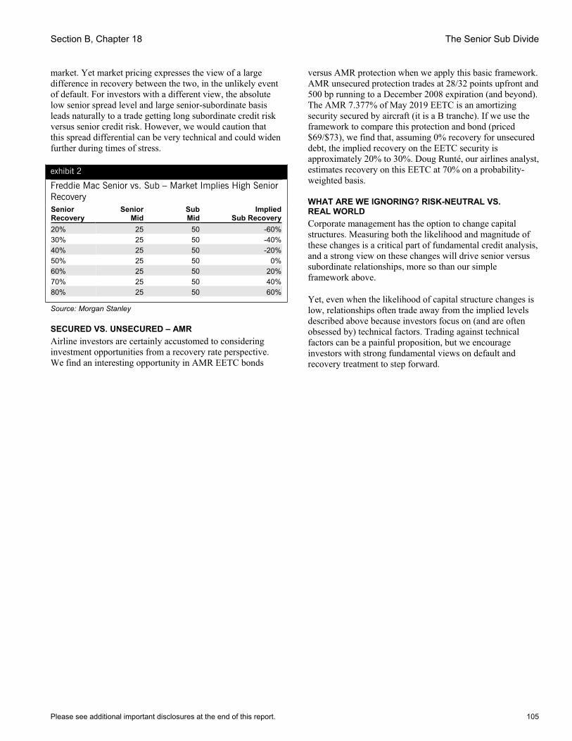
Section B, Chapter 18 The Senior Sub Divide
Please see additional important disclosures at the end of this report. 105
market. Yet market pricing expresses the view of a large difference in recovery between the two, in the unlikely event of default. For investors with a different view, the absolute low senior spread level and large senior-subordinate basis leads naturally to a trade getting long subordinate credit risk versus senior credit risk. However, we would caution that this spread differential can be very technical and could widen further during times of stress.
exhibit 2
Freddie Mac Senior vs. Sub – Market Implies High Senior RecoverySeniorRecovery
SeniorMid
SubMid
Implied Sub Recovery
20% 25 50 -60%30% 25 50 -40%40% 25 50 -20%50% 25 50 0%60% 25 50 20%70% 25 50 40%80% 25 50 60%
Source: Morgan Stanley
SECURED VS. UNSECURED – AMR Airline investors are certainly accustomed to considering investment opportunities from a recovery rate perspective. We find an interesting opportunity in AMR EETC bonds
versus AMR protection when we apply this basic framework. AMR unsecured protection trades at 28/32 points upfront and 500 bp running to a December 2008 expiration (and beyond). The AMR 7.377% of May 2019 EETC is an amortizing security secured by aircraft (it is a B tranche). If we use the framework to compare this protection and bond (priced $69/$73), we find that, assuming 0% recovery for unsecured debt, the implied recovery on the EETC security is approximately 20% to 30%. Doug Runté, our airlines analyst, estimates recovery on this EETC at 70% on a probability-weighted basis.
WHAT ARE WE IGNORING? RISK-NEUTRAL VS. REAL WORLD Corporate management has the option to change capital structures. Measuring both the likelihood and magnitude of these changes is a critical part of fundamental credit analysis, and a strong view on these changes will drive senior versus subordinate relationships, more so than our simple framework above.
Yet, even when the likelihood of capital structure changes is low, relationships often trade away from the implied levels described above because investors focus on (and are often obsessed by) technical factors. Trading against technical factors can be a painful proposition, but we encourage investors with strong fundamental views on default and recovery treatment to step forward.
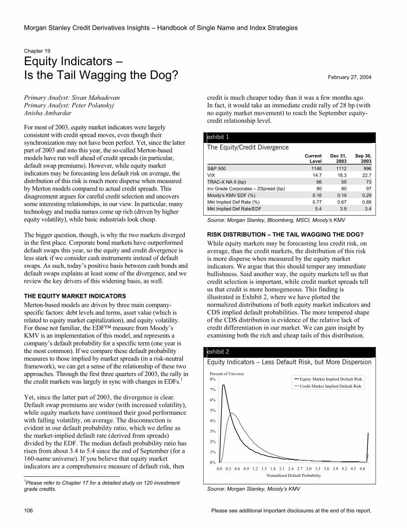
Morgan Stanley Credit Derivatives Insights – Handbook of Single Name and Index Strategies
106 Please see additional important disclosures at the end of this report.
Chapter 19
Equity Indicators –Is the Tail Wagging the Dog? February 27, 2004
Primary Analyst: Sivan Mahadevan Primary Analyst: Peter Polanskyj Anisha Ambardar
For most of 2003, equity market indicators were largely consistent with credit spread moves, even though their synchronization may not have been perfect. Yet, since the latter part of 2003 and into this year, the so-called Merton-based models have run well ahead of credit spreads (in particular, default swap premiums). However, while equity market indicators may be forecasting less default risk on average, the distribution of this risk is much more disperse when measured by Merton models compared to actual credit spreads. This disagreement argues for careful credit selection and uncovers some interesting relationships, in our view. In particular, many technology and media names come up rich (driven by higher equity volatility), while basic industrials look cheap.
The bigger question, though, is why the two markets diverged in the first place. Corporate bond markets have outperformed default swaps this year, so the equity and credit divergence is less stark if we consider cash instruments instead of default swaps. As such, today’s positive basis between cash bonds and default swaps explains at least some of the divergence, and we review the key drivers of this widening basis, as well.
THE EQUITY MARKET INDICATORS Merton-based models are driven by three main company-specific factors: debt levels and terms, asset value (which is related to equity market capitalization), and equity volatility. For those not familiar, the EDF™ measure from Moody’s KMV is an implementation of this model, and represents a company’s default probability for a specific term (one year is the most common). If we compare these default probability measures to those implied by market spreads (in a risk-neutral framework), we can get a sense of the relationship of these two approaches. Through the first three quarters of 2003, the rally in the credit markets was largely in sync with changes in EDFs.1
Yet, since the latter part of 2003, the divergence is clear. Default swap premiums are wider (with increased volatility), while equity markets have continued their good performance with falling volatility, on average. The disconnection is evident in our default probability ratio, which we define as the market-implied default rate (derived from spreads) divided by the EDF. The median default probability ratio has risen from about 3.4 to 5.4 since the end of September (for a 160-name universe). If you believe that equity market indicators are a comprehensive measure of default risk, then 1Please refer to Chapter 17 for a detailed study on 120 investment grade credits.
credit is much cheaper today than it was a few months ago. In fact, it would take an immediate credit rally of 28 bp (with no equity market movement) to reach the September equity-credit relationship level.
exhibit 1
The Equity/Credit Divergence Current
Level Dec 31,
2003Sep 30,
2003S&P 500 1146 1112 996VIX 14.7 18.3 22.7TRAC-X NA II (bp) 66 55 73Inv Grade Corporates – ZSpread (bp) 80 80 97Moody’s KMV EDF (%) 0.16 0.19 0.29Mkt Implied Def Rate (%) 0.77 0.67 0.88Mkt Implied Def Rate/EDF 5.4 3.9 3.4
Source: Morgan Stanley, Bloomberg, MSCI, Moody’s KMV
RISK DISTRIBUTION – THE TAIL WAGGING THE DOG? While equity markets may be forecasting less credit risk, on average, than the credit markets, the distribution of this risk is more disperse when measured by the equity market indicators. We argue that this should temper any immediate bullishness. Said another way, the equity markets tell us that credit selection is important, while credit market spreads tell us that credit is more homogeneous. This finding is illustrated in Exhibit 2, where we have plotted the normalized distributions of both equity market indicators and CDS implied default probabilities. The more tempered shape of the CDS distribution is evidence of the relative lack of credit differentiation in our market. We can gain insight by examining both the rich and cheap tails of this distribution.
exhibit 2
Equity Indicators – Less Default Risk, but More Dispersion
Percent of Universe
0%
1%
2%
3%
4%
5%
6%
7%
8%
0.0 0.3 0.6 0.9 1.2 1.5 1.8 2.1 2.4 2.7 3.0 3.3 3.6 3.9 4.2 4.5 4.8Normalized Default Probability
Equity Market Implied Default Risk
Credit Market Implied Default Risk
Source: Morgan Stanley, Moody’s KMV
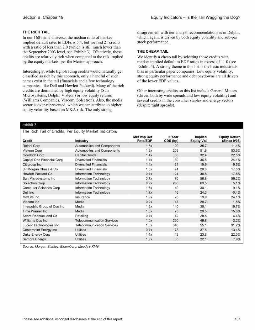
Section B, Chapter 19 Equity Indicators – Is the Tail Wagging the Dog?
Please see additional important disclosures at the end of this report. 107
THE RICH TAIL In our 160-name universe, the median ratio of market-implied default rates to EDFs is 5.4, but we find 21 credits with a ratio of less than 2.0 (which is still much lower than the September 2003 level, see Exhibit 3). Effectively, these credits are relatively rich when compared to the risk implied by the equity markets, per the Merton approach.
Interestingly, while tight-trading credits would naturally get classified as rich by this approach, only a handful of such names exist in the tail (financials and a few technology companies, like Dell and Hewlett Packard). Many of the rich credits are dominated by high equity volatility (Sun Microsystems, Delphi, Visteon) or low equity returns (Williams Companies, Viacom, Solectron). Also, the media sector is over-represented, which we can attribute to higher equity volatility based on M&A risk. The only strong
disagreement with our analyst recommendations is in Delphi, which, again, is driven by both equity volatility and sub-par stock performance.
THE CHEAP TAIL We identify a cheap tail by selecting those credits with market-implied default to EDF ratios in excess of 11.0 (see Exhibit 4). A strong theme in this list is the basic industrials bias in particular paper companies. Low equity volatility, strong equity performance and debt paydowns are all drivers of the lower EDF values.
Other interesting credits on this list include General Motors (driven both by wide spreads and low equity volatility) and several credits in the consumer staples and energy sectors (despite tight spreads).
exhibit 3
The Rich Tail of Credits, Per Equity Market Indicators
Credit Industry Mkt Imp Def
Rate/EDF5 Year
CDS (bp)Implied
Equity VolEquity Return
(Since 9/03)Delphi Corp Automobiles and Components 1.8x 100 35.7 11.4%Visteon Corp Automobiles and Components 1.8x 203 51.8 53.6%Goodrich Corp Capital Goods 1.4x 63 32.4 22.5%Capital One Financial Corp Diversified Financials 1.1x 60 36.5 24.1%Citigroup Inc Diversified Financials 1.4x 21 19.9 9.5%JP Morgan Chase & Co Diversified Financials 1.6x 24 20.6 17.5%Hewlett-Packard Co Information Technology 0.7x 24 30.8 17.5%Sun Microsystems Inc Information Technology 0.7x 75 56.8 56.2%Solectron Corp Information Technology 0.9x 280 69.5 5.1%Computer Sciences Corp Information Technology 1.6x 40 30.1 9.1%Dell Inc Information Technology 1.7x 16 24.3 -0.4%MetLife Inc Insurance 1.9x 25 19.9 24.1%Viacom Inc Media 0.2x 47 29.7 1.8%Interpublic Group of Cos Inc Media 1.6x 140 35.1 19.7%Time Warner Inc Media 1.8x 73 29.5 15.6%Sears Roebuck and Co Retailing 0.7x 42 28.5 6.4%Williams Cos Inc Telecommunication Services 1.0x 250 49.8 -2.2%Lucent Technologies Inc Telecommunication Services 1.6x 340 55.1 91.2%Centerpoint Energy Inc Utilities 0.7x 178 37.6 13.4%Duke Energy Corp Utilities 1.1x 43 23.8 22.0%Sempra Energy Utilities 1.9x 35 22.1 7.9%
Source: Morgan Stanley, Bloomberg, Moody’s KMV
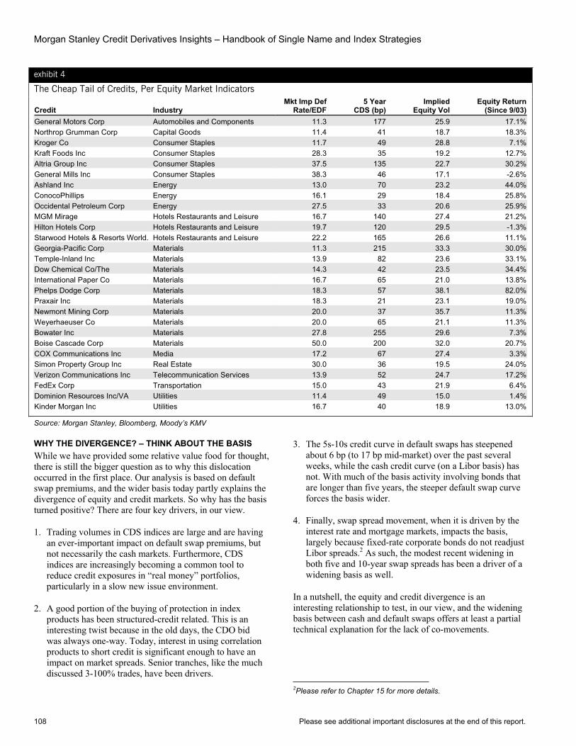
Morgan Stanley Credit Derivatives Insights – Handbook of Single Name and Index Strategies
108 Please see additional important disclosures at the end of this report.
exhibit 4
The Cheap Tail of Credits, Per Equity Market Indicators
Credit Industry Mkt Imp Def
Rate/EDF5 Year
CDS (bp)Implied
Equity Vol Equity Return
(Since 9/03)General Motors Corp Automobiles and Components 11.3 177 25.9 17.1%Northrop Grumman Corp Capital Goods 11.4 41 18.7 18.3%Kroger Co Consumer Staples 11.7 49 28.8 7.1%Kraft Foods Inc Consumer Staples 28.3 35 19.2 12.7%Altria Group Inc Consumer Staples 37.5 135 22.7 30.2%General Mills Inc Consumer Staples 38.3 46 17.1 -2.6%Ashland Inc Energy 13.0 70 23.2 44.0%ConocoPhillips Energy 16.1 29 18.4 25.8%Occidental Petroleum Corp Energy 27.5 33 20.6 25.9%MGM Mirage Hotels Restaurants and Leisure 16.7 140 27.4 21.2%Hilton Hotels Corp Hotels Restaurants and Leisure 19.7 120 29.5 -1.3%Starwood Hotels & Resorts World. Hotels Restaurants and Leisure 22.2 165 26.6 11.1%Georgia-Pacific Corp Materials 11.3 215 33.3 30.0%Temple-Inland Inc Materials 13.9 82 23.6 33.1%Dow Chemical Co/The Materials 14.3 42 23.5 34.4%International Paper Co Materials 16.7 65 21.0 13.8%Phelps Dodge Corp Materials 18.3 57 38.1 82.0%Praxair Inc Materials 18.3 21 23.1 19.0%Newmont Mining Corp Materials 20.0 37 35.7 11.3%Weyerhaeuser Co Materials 20.0 65 21.1 11.3%Bowater Inc Materials 27.8 255 29.6 7.3%Boise Cascade Corp Materials 50.0 200 32.0 20.7%COX Communications Inc Media 17.2 67 27.4 3.3%Simon Property Group Inc Real Estate 30.0 36 19.5 24.0%Verizon Communications Inc Telecommunication Services 13.9 52 24.7 17.2%FedEx Corp Transportation 15.0 43 21.9 6.4%Dominion Resources Inc/VA Utilities 11.4 49 15.0 1.4%Kinder Morgan Inc Utilities 16.7 40 18.9 13.0%
Source: Morgan Stanley, Bloomberg, Moody’s KMV
WHY THE DIVERGENCE? – THINK ABOUT THE BASIS While we have provided some relative value food for thought, there is still the bigger question as to why this dislocation occurred in the first place. Our analysis is based on default swap premiums, and the wider basis today partly explains the divergence of equity and credit markets. So why has the basis turned positive? There are four key drivers, in our view.
1. Trading volumes in CDS indices are large and are having an ever-important impact on default swap premiums, but not necessarily the cash markets. Furthermore, CDS indices are increasingly becoming a common tool to reduce credit exposures in “real money” portfolios, particularly in a slow new issue environment.
2. A good portion of the buying of protection in index products has been structured-credit related. This is an interesting twist because in the old days, the CDO bid was always one-way. Today, interest in using correlation products to short credit is significant enough to have an impact on market spreads. Senior tranches, like the much discussed 3-100% trades, have been drivers.
3. The 5s-10s credit curve in default swaps has steepened about 6 bp (to 17 bp mid-market) over the past several weeks, while the cash credit curve (on a Libor basis) has not. With much of the basis activity involving bonds that are longer than five years, the steeper default swap curve forces the basis wider.
4. Finally, swap spread movement, when it is driven by the interest rate and mortgage markets, impacts the basis, largely because fixed-rate corporate bonds do not readjust Libor spreads.2 As such, the modest recent widening in both five and 10-year swap spreads has been a driver of a widening basis as well.
In a nutshell, the equity and credit divergence is an interesting relationship to test, in our view, and the widening basis between cash and default swaps offers at least a partial technical explanation for the lack of co-movements.
2Please refer to Chapter 15 for more details.
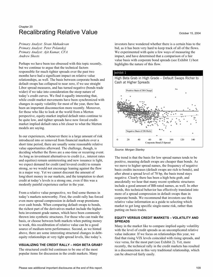
Please see additional important disclosures at the end of this report. 109
Chapter 20
Recalibrating Relative Value October 15, 2004
Primary Analyst: Sivan Mahadevan Primary Analyst: Peter Polanskyj Primary Analyst: Ajit Kumar, CFA Andrew Sheets
Perhaps we have been too obsessed with this topic recently, but we continue to argue that the technical factors responsible for much tighter spreads over the past two months have had a significant impact on relative value relationships, as well. The basis between corporate bonds and default swaps has collapsed to near zero, if we use straight Libor spread measures, and has turned negative (bonds trade wider) if we take into consideration the steep nature of today’s credit curves. We find it equally interesting that, while credit market movements have been synchronized with changes in equity volatility for most of the year, there has been an important disconnection more recently. Moreover, for those who like to look at the world from a Merton perspective, equity-market implied default rates continue to be quite low, and tighter spreads have now forced credit-market implied default rates a bit closer to what the Merton models are saying.
In our experiences, whenever there is a large amount of risk introduced into or removed from financial markets over a short time period, there are usually some reasonable relative value opportunities afterward. The challenge, though, is deciding whether the flows are a one-time or recurring event. As long as investment alternatives to credit (i.e., interest rates and equities) remain uninteresting and new issuance is light, we expect demand for credit (and levered credit) to remain strong, so we would not encourage leaning against the flow in a major way. Yet we cannot discount the amount of long/short money in our markets, and the temptation to short credit at today’s levels is a strong one, even if this was a modestly painful experience earlier in the year.
From a relative value perspective, we find some themes in today’s markets noteworthy. First, the credit rally has forced even more spread compression in default swap premiums over cash bonds. When comparing default swaps to bonds, the richest part of the derivatives market include the higher-beta investment grade names, which have been commonly thrown into synthetic structures. For those who can trade the basis, or choose between both markets when putting money to work, this recalibration of relative value can be a good source of medium-term performance. Second, as we hinted above, there are some interesting structural changes in debt-equity relationships at very tight spread levels, like today’s.
VISUALIZING THE CREDIT RALLY – HIGH BETA GRAB? The structured credit bid continues to be one of the most popular items for discussion in the credit markets. Many
investors have wondered whether there is a certain bias to the bid, as it has been very hard to keep track of all of the flows. We experimented with quite a few ways of measuring the impact, and have determined that a comparison of a fair value basis with corporate bond spreads (see Exhibit 1) best highlights the nature of this flow.
exhibit 1
High Beta Grab in High Grade – Default Swaps Richer to Cash at Higher Spreads
0 20 40 60 80 100 120 140Corporate Bond Z-Spread
Positive Basis (CDS Cheap)
Negative Basis (CDS Rich)
Source: Morgan Stanley
The trend is that the basis for low spread names tends to be positive, meaning default swaps are cheaper than bonds. As we move to higher spread names, the frequency of negative basis credits increases (default swaps are rich to bonds), and after about a spread level of 70 bp, the basis trend stays negative. Clearly there has been a high beta grab, and anecdotally we hear that many recent synthetic structures include a good amount of BB-rated names, as well. In other words, this technical behavior has effectively translated into more of a spread compression in default swaps than in corporate bonds. We recommend that investors use this relative value information as a guide to selecting which market to get long specific single-name risk, rather than putting on basis trades.
EQUITY VERSUS CREDIT MARKETS – VOLATILITY AND SPREADS Many in the market like to compare implied equity volatility with the level of credit spreads as an uncomplicated relative value indicator. If we focus on relationships this year, we find that rising VIX levels coincided with rising spreads, and vice versa, for the most part (see Exhibit 2). Yet, more recently, the technical rally in the credit markets has resulted in a disconnection in this very traditional relationship, which can be observed fairly easily.
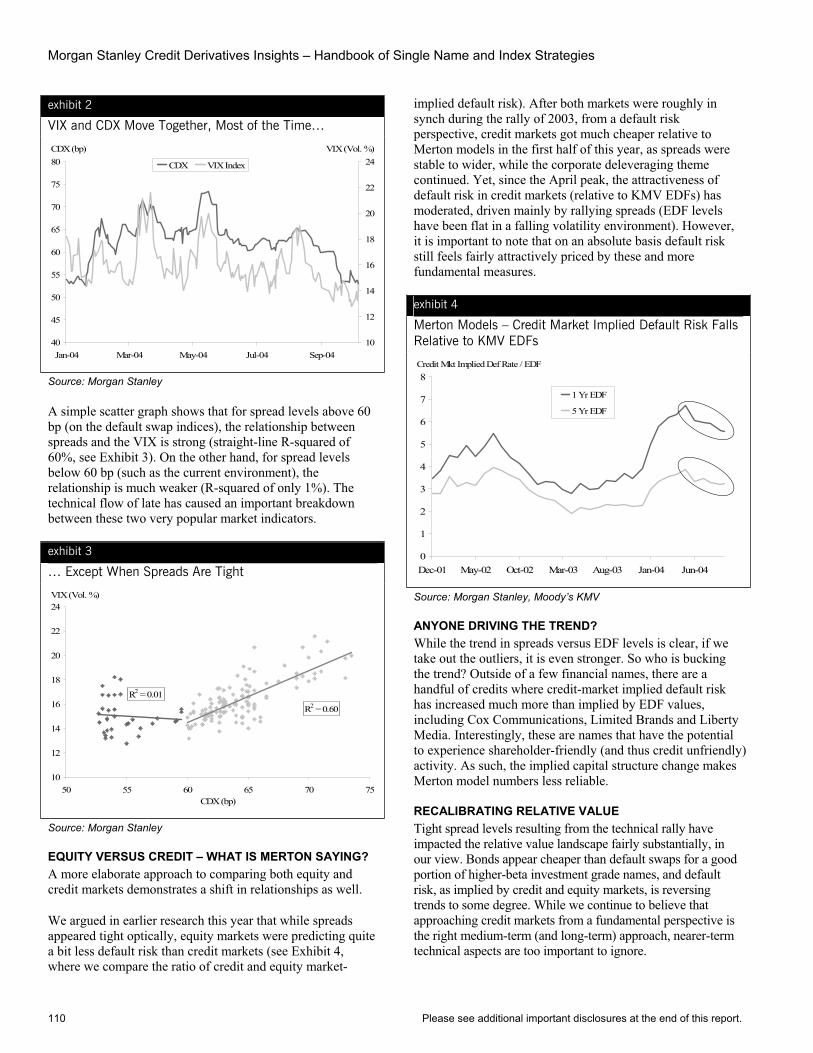
Morgan Stanley Credit Derivatives Insights – Handbook of Single Name and Index Strategies
110 Please see additional important disclosures at the end of this report.
exhibit 2
VIX and CDX Move Together, Most of the Time…
40
45
50
55
60
65
70
75
80
Jan-04 Mar-04 May-04 Jul-04 Sep-04
CDX (bp)
10
12
14
16
18
20
22
24VIX (Vol. %)
CDX VIX Index
Source: Morgan Stanley
A simple scatter graph shows that for spread levels above 60 bp (on the default swap indices), the relationship between spreads and the VIX is strong (straight-line R-squared of 60%, see Exhibit 3). On the other hand, for spread levels below 60 bp (such as the current environment), the relationship is much weaker (R-squared of only 1%). The technical flow of late has caused an important breakdown between these two very popular market indicators.
exhibit 3
… Except When Spreads Are Tight
10
12
14
16
18
20
22
24
50 55 60 65 70 75CDX (bp)
VIX (Vol. %)
R2 = 0.01
R2 = 0.60
Source: Morgan Stanley
EQUITY VERSUS CREDIT – WHAT IS MERTON SAYING? A more elaborate approach to comparing both equity and credit markets demonstrates a shift in relationships as well.
We argued in earlier research this year that while spreads appeared tight optically, equity markets were predicting quite a bit less default risk than credit markets (see Exhibit 4, where we compare the ratio of credit and equity market-
implied default risk). After both markets were roughly in synch during the rally of 2003, from a default risk perspective, credit markets got much cheaper relative to Merton models in the first half of this year, as spreads were stable to wider, while the corporate deleveraging theme continued. Yet, since the April peak, the attractiveness of default risk in credit markets (relative to KMV EDFs) has moderated, driven mainly by rallying spreads (EDF levels have been flat in a falling volatility environment). However, it is important to note that on an absolute basis default risk still feels fairly attractively priced by these and more fundamental measures.
exhibit 4
Merton Models – Credit Market Implied Default Risk Falls Relative to KMV EDFs
Credit Mkt Implied Def Rate / EDF
0
1
2
3
4
5
6
7
8
Dec-01 May-02 Oct-02 Mar-03 Aug-03 Jan-04 Jun-04
1 Yr EDF
5 Yr EDF
Source: Morgan Stanley, Moody’s KMV
ANYONE DRIVING THE TREND? While the trend in spreads versus EDF levels is clear, if we take out the outliers, it is even stronger. So who is bucking the trend? Outside of a few financial names, there are a handful of credits where credit-market implied default risk has increased much more than implied by EDF values, including Cox Communications, Limited Brands and Liberty Media. Interestingly, these are names that have the potential to experience shareholder-friendly (and thus credit unfriendly) activity. As such, the implied capital structure change makes Merton model numbers less reliable.
RECALIBRATING RELATIVE VALUE Tight spread levels resulting from the technical rally have impacted the relative value landscape fairly substantially, in our view. Bonds appear cheaper than default swaps for a good portion of higher-beta investment grade names, and default risk, as implied by credit and equity markets, is reversing trends to some degree. While we continue to believe that approaching credit markets from a fundamental perspective is the right medium-term (and long-term) approach, nearer-term technical aspects are too important to ignore.
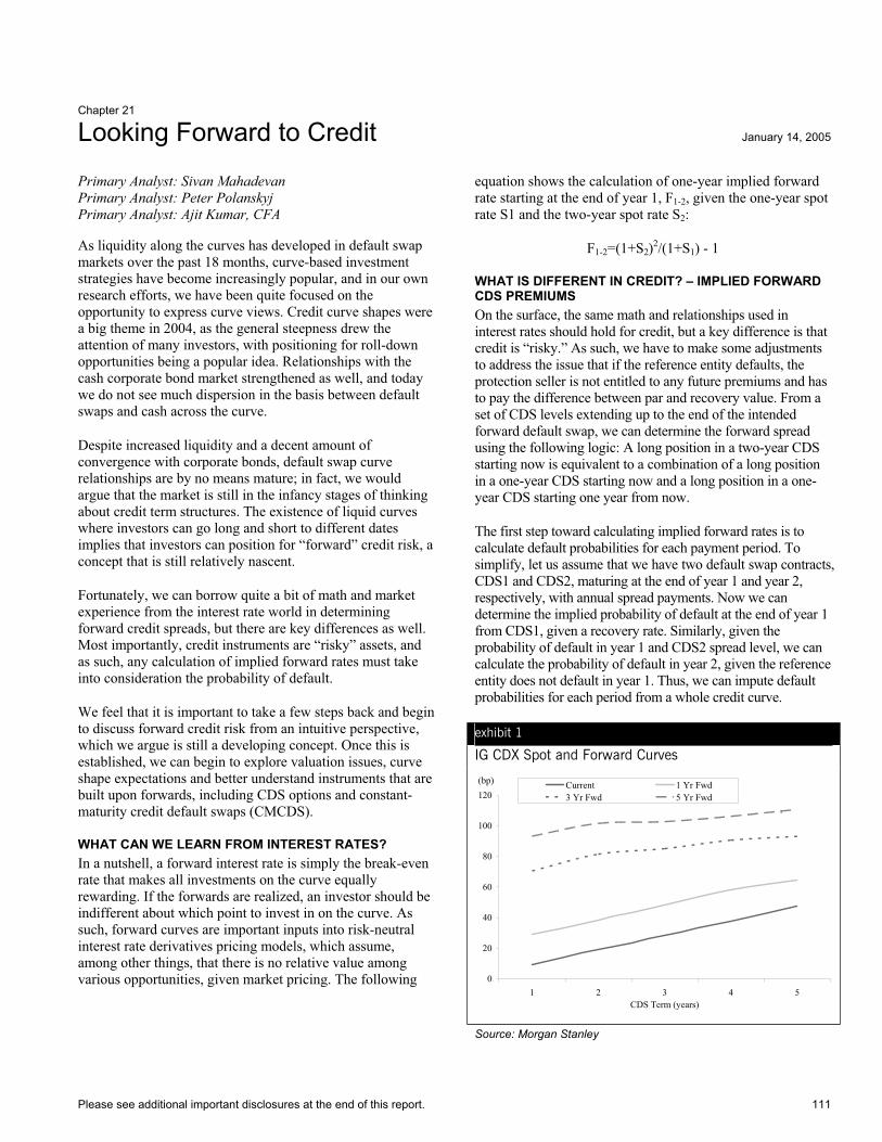
Please see additional important disclosures at the end of this report. 111
Chapter 21
Looking Forward to Credit January 14, 2005
Primary Analyst: Sivan Mahadevan Primary Analyst: Peter Polanskyj Primary Analyst: Ajit Kumar, CFA
As liquidity along the curves has developed in default swap markets over the past 18 months, curve-based investment strategies have become increasingly popular, and in our own research efforts, we have been quite focused on the opportunity to express curve views. Credit curve shapes were a big theme in 2004, as the general steepness drew the attention of many investors, with positioning for roll-down opportunities being a popular idea. Relationships with the cash corporate bond market strengthened as well, and today we do not see much dispersion in the basis between default swaps and cash across the curve.
Despite increased liquidity and a decent amount of convergence with corporate bonds, default swap curve relationships are by no means mature; in fact, we would argue that the market is still in the infancy stages of thinking about credit term structures. The existence of liquid curves where investors can go long and short to different dates implies that investors can position for “forward” credit risk, a concept that is still relatively nascent.
Fortunately, we can borrow quite a bit of math and market experience from the interest rate world in determining forward credit spreads, but there are key differences as well. Most importantly, credit instruments are “risky” assets, and as such, any calculation of implied forward rates must take into consideration the probability of default.
We feel that it is important to take a few steps back and begin to discuss forward credit risk from an intuitive perspective, which we argue is still a developing concept. Once this is established, we can begin to explore valuation issues, curve shape expectations and better understand instruments that are built upon forwards, including CDS options and constant-maturity credit default swaps (CMCDS).
WHAT CAN WE LEARN FROM INTEREST RATES? In a nutshell, a forward interest rate is simply the break-even rate that makes all investments on the curve equally rewarding. If the forwards are realized, an investor should be indifferent about which point to invest in on the curve. As such, forward curves are important inputs into risk-neutral interest rate derivatives pricing models, which assume, among other things, that there is no relative value among various opportunities, given market pricing. The following
equation shows the calculation of one-year implied forward rate starting at the end of year 1, F1-2, given the one-year spot rate S1 and the two-year spot rate S2:
F1-2=(1+S2)2/(1+S1) - 1
WHAT IS DIFFERENT IN CREDIT? – IMPLIED FORWARD CDS PREMIUMS On the surface, the same math and relationships used in interest rates should hold for credit, but a key difference is that credit is “risky.” As such, we have to make some adjustments to address the issue that if the reference entity defaults, the protection seller is not entitled to any future premiums and has to pay the difference between par and recovery value. From a set of CDS levels extending up to the end of the intended forward default swap, we can determine the forward spread using the following logic: A long position in a two-year CDS starting now is equivalent to a combination of a long position in a one-year CDS starting now and a long position in a one-year CDS starting one year from now.
The first step toward calculating implied forward rates is to calculate default probabilities for each payment period. To simplify, let us assume that we have two default swap contracts, CDS1 and CDS2, maturing at the end of year 1 and year 2, respectively, with annual spread payments. Now we can determine the implied probability of default at the end of year 1 from CDS1, given a recovery rate. Similarly, given the probability of default in year 1 and CDS2 spread level, we can calculate the probability of default in year 2, given the reference entity does not default in year 1. Thus, we can impute default probabilities for each period from a whole credit curve.
exhibit 1
IG CDX Spot and Forward Curves
(bp)
0
20
40
60
80
100
120
1 2 3 4 5CDS Term (years)
Current 1 Yr Fwd3 Yr Fwd 5 Yr Fwd
Source: Morgan Stanley

Morgan Stanley Credit Derivatives Insights – Handbook of Single Name and Index Strategies
112 Please see additional important disclosures at the end of this report.
The combination of CDS1 and a forward default swap, which starts at the end of year 1, replicates CDS2. Therefore, by equating the two cashflow streams, we can determine the implied forward default swap level. We show spot and selected forward curves for the CDX index curve in Exhibit 1.
FORWARDS – A DOSE OF REALITY How realistic are implied forward credit spreads? On a credit-specific basis, almost any curve shape, from very steep to inverted, is justifiable. Distressed credits tend to have inverted curves because of the pari passu claim that bonds of the same seniority (but different terms) have on assets. Market-wide investment grade credit curves (As and BBBs) have indeed been inverted during the worst parts of past credit cycles (1991 and 2002, see Exhibit 2), although the inversion in both periods did not last very long.
exhibit 2
Flat to Inverted Credit Curves Have Occurred at Much Wider Spreads (BBBs)
-200
-150
-100
-50
0
50
100
150
200
Jan-89 Mar-92 May-95 Aug-98 Oct-01 Jan-05
bp
-500
-400
-300
-200
-100
0
100
200
300
400
500bp
2's-5's Curve (Left Axis)
5's-10's Curve (Left Axis)
5yr Libor Spread (Right Axis)
Source: Morgan Stanley, The YieldBook
Forwards in interest rate markets have tended to overestimate the realized rates (providing evidence of an increasing risk premium for taking longer-duration rate risk). The implied forwards in the credit markets may reflect the expected future spread, as well as the risk premium for taking longer-dated credit risk. Even more so than the interest rate markets, the risk premium associated with taking credit risk with varying maturities can be highly volatile over time and can also vary substantially by credit.
TRADING AGAINST THE CREDIT FORWARDS While forwards are important inputs into risk-neutral pricing models, forwards rarely get realized, and as such, strategies that lean against the forwards can be interesting ways to implement both credit-specific and macro credit views over time.
Today’s steep curves imply relatively flat front-end credit curves 4 to 5 years forward (see Exhibit 1), which, based on historical experience, would suggest a time of substantially increased credit risk. If the forwards are correct from a curve shape perspective, we would argue that spreads ought to be wider than implied by the forwards (based on historical experience, see Exhibit 2). One credit-based argument for this view is that, in investment grade, there tends to be a net negative ratings migration over time, which is an argument against curves staying flat or inverted at relatively tight spread levels.1
Furthermore, the linkage between curve shape and absolute spread has intuitive appeal when we consider how investors will perceive credit risk across the term structure. When credit fundamentals are strong and spreads tight (like today), investors will be very comfortable with credit risk in the short end but will charge some incremental premium for longer-dated risk because of a lack of clarity on business conditions or corporate actions in the long term. In times of financial uncertainty and wide spreads, investors will have a lack of clarity over the short term and will charge a large risk premium even for short-dated risk. Longer-dated risk, on the other hand, may be viewed as marginally less risky, as investors view survival in the short term as the key business risk (consider the airlines over the last year).
PUTTING ON THE FLATTENER – AT WHAT COST? For investors who disagree with the forwards, there are many ways to implement the views, including curve trades and products built upon forwards like options and constant-maturity default swaps. The curve flattening trade is both tempting and rather popular today, and as such, we chose to study three simple flattening trades in the CDX index (sell long-dated protection, buy shorter-dated protection, duration neutral) as ways to position against the forwards. In particular, there are two points worth noting. First, unlike in the interest rate world, a trade that is not notionally neutral has an added risk, namely, the default risk on the incremental difference in notional values. In the case of flatteners, this will imply a positive default P/L. Second, the spread duration of each leg will drift over time, but not uniformly, which will lead to residual spread exposures over time (see Exhibit 3).
1Please refer to Chapter 50.
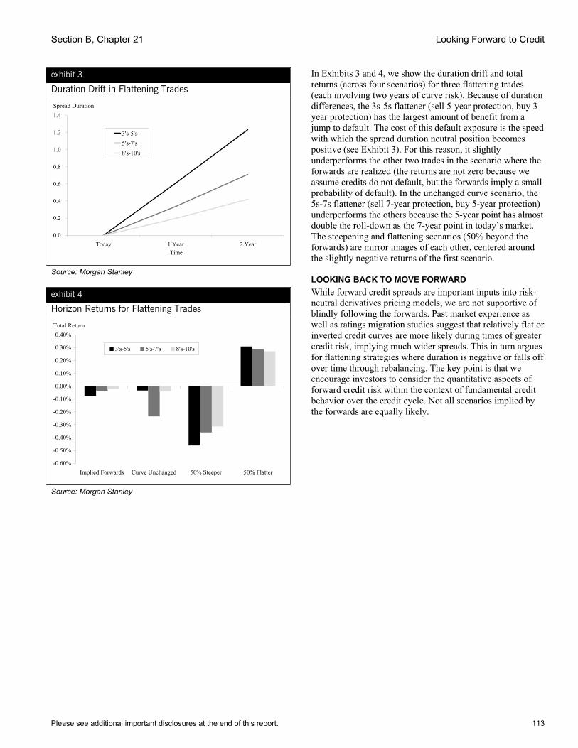
Section B, Chapter 21 Looking Forward to Credit
Please see additional important disclosures at the end of this report. 113
exhibit 3
Duration Drift in Flattening Trades
Spread Duration
0.0
0.2
0.4
0.6
0.8
1.0
1.2
1.4
Today 1 Year 2 YearTime
3's-5's5's-7's8's-10's
Source: Morgan Stanley
exhibit 4
Horizon Returns for Flattening Trades
Total Return
-0.60%
-0.50%
-0.40%
-0.30%
-0.20%
-0.10%
0.00%
0.10%
0.20%
0.30%
0.40%
Implied Forwards Curve Unchanged 50% Steeper 50% Flatter
3's-5's 5's-7's 8's-10's
Source: Morgan Stanley
In Exhibits 3 and 4, we show the duration drift and total returns (across four scenarios) for three flattening trades (each involving two years of curve risk). Because of duration differences, the 3s-5s flattener (sell 5-year protection, buy 3-year protection) has the largest amount of benefit from a jump to default. The cost of this default exposure is the speed with which the spread duration neutral position becomes positive (see Exhibit 3). For this reason, it slightly underperforms the other two trades in the scenario where the forwards are realized (the returns are not zero because we assume credits do not default, but the forwards imply a small probability of default). In the unchanged curve scenario, the 5s-7s flattener (sell 7-year protection, buy 5-year protection) underperforms the others because the 5-year point has almost double the roll-down as the 7-year point in today’s market. The steepening and flattening scenarios (50% beyond the forwards) are mirror images of each other, centered around the slightly negative returns of the first scenario.
LOOKING BACK TO MOVE FORWARD While forward credit spreads are important inputs into risk-neutral derivatives pricing models, we are not supportive of blindly following the forwards. Past market experience as well as ratings migration studies suggest that relatively flat or inverted credit curves are more likely during times of greater credit risk, implying much wider spreads. This in turn argues for flattening strategies where duration is negative or falls off over time through rebalancing. The key point is that we encourage investors to consider the quantitative aspects of forward credit risk within the context of fundamental credit behavior over the credit cycle. Not all scenarios implied by the forwards are equally likely.
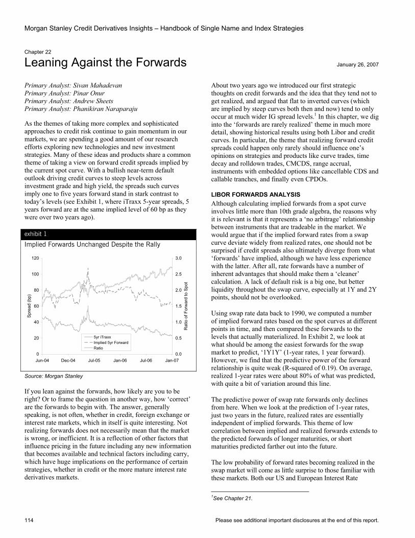
Morgan Stanley Credit Derivatives Insights – Handbook of Single Name and Index Strategies
114 Please see additional important disclosures at the end of this report.
Chapter 22
Leaning Against the Forwards January 26, 2007
Primary Analyst: Sivan Mahadevan Primary Analyst: Pinar Onur Primary Analyst: Andrew Sheets Primary Analyst: Phanikiran Naraparaju
As the themes of taking more complex and sophisticated approaches to credit risk continue to gain momentum in our markets, we are spending a good amount of our research efforts exploring new technologies and new investment strategies. Many of these ideas and products share a common theme of taking a view on forward credit spreads implied by the current spot curve. With a bullish near-term default outlook driving credit curves to steep levels across investment grade and high yield, the spreads such curves imply one to five years forward stand in stark contrast to today’s levels (see Exhibit 1, where iTraxx 5-year spreads, 5 years forward are at the same implied level of 60 bp as they were over two years ago).
exhibit 1
Implied Forwards Unchanged Despite the Rally
0
20
40
60
80
100
120
Jun-04 Dec-04 Jul-05 Jan-06 Jul-06 Jan-07
Spre
ad (b
p)
0.0
0.5
1.0
1.5
2.0
2.5
3.0
Rat
io o
f For
war
d to
Spo
t
5yr iTraxxImplied 5yr ForwardRatio
Source: Morgan Stanley
If you lean against the forwards, how likely are you to be right? Or to frame the question in another way, how ‘correct’ are the forwards to begin with. The answer, generally speaking, is not often, whether in credit, foreign exchange or interest rate markets, which in itself is quite interesting. Not realizing forwards does not necessarily mean that the market is wrong, or inefficient. It is a reflection of other factors that influence pricing in the future including any new information that becomes available and technical factors including carry, which have huge implications on the performance of certain strategies, whether in credit or the more mature interest rate derivatives markets.
About two years ago we introduced our first strategic thoughts on credit forwards and the idea that they tend not to get realized, and argued that flat to inverted curves (which are implied by steep curves both then and now) tend to only occur at much wider IG spread levels.1 In this chapter, we dig into the ‘forwards are rarely realized’ theme in much more detail, showing historical results using both Libor and credit curves. In particular, the theme that realizing forward credit spreads could happen only rarely should influence one’s opinions on strategies and products like curve trades, time decay and rolldown trades, CMCDS, range accrual, instruments with embedded options like cancellable CDS and callable tranches, and finally even CPDOs.
LIBOR FORWARDS ANALYSIS Although calculating implied forwards from a spot curve involves little more than 10th grade algebra, the reasons why it is relevant is that it represents a ‘no arbitrage’ relationship between instruments that are tradeable in the market. We would argue that if the implied forward rates from a swap curve deviate widely from realized rates, one should not be surprised if credit spreads also ultimately diverge from what ‘forwards’ have implied, although we have less experience with the latter. After all, rate forwards have a number of inherent advantages that should make them a ‘cleaner’ calculation. A lack of default risk is a big one, but better liquidity throughout the swap curve, especially at 1Y and 2Y points, should not be overlooked.
Using swap rate data back to 1990, we computed a number of implied forward rates based on the spot curves at different points in time, and then compared these forwards to the levels that actually materialized. In Exhibit 2, we look at what should be among the easiest forwards for the swap market to predict, ‘1Y1Y’ (1-year rates, 1 year forward). However, we find that the predictive power of the forward relationship is quite weak (R-squared of 0.19). On average, realized 1-year rates were about 80% of what was predicted, with quite a bit of variation around this line.
The predictive power of swap rate forwards only declines from here. When we look at the prediction of 1-year rates, just two years in the future, realized rates are essentially independent of implied forwards. This theme of low correlation between implied and realized forwards extends to the predicted forwards of longer maturities, or short maturities predicted farther out into the future.
The low probability of forward rates becoming realized in the swap market will come as little surprise to those familiar with these markets. Both our US and European Interest Rate
1See Chapter 21.
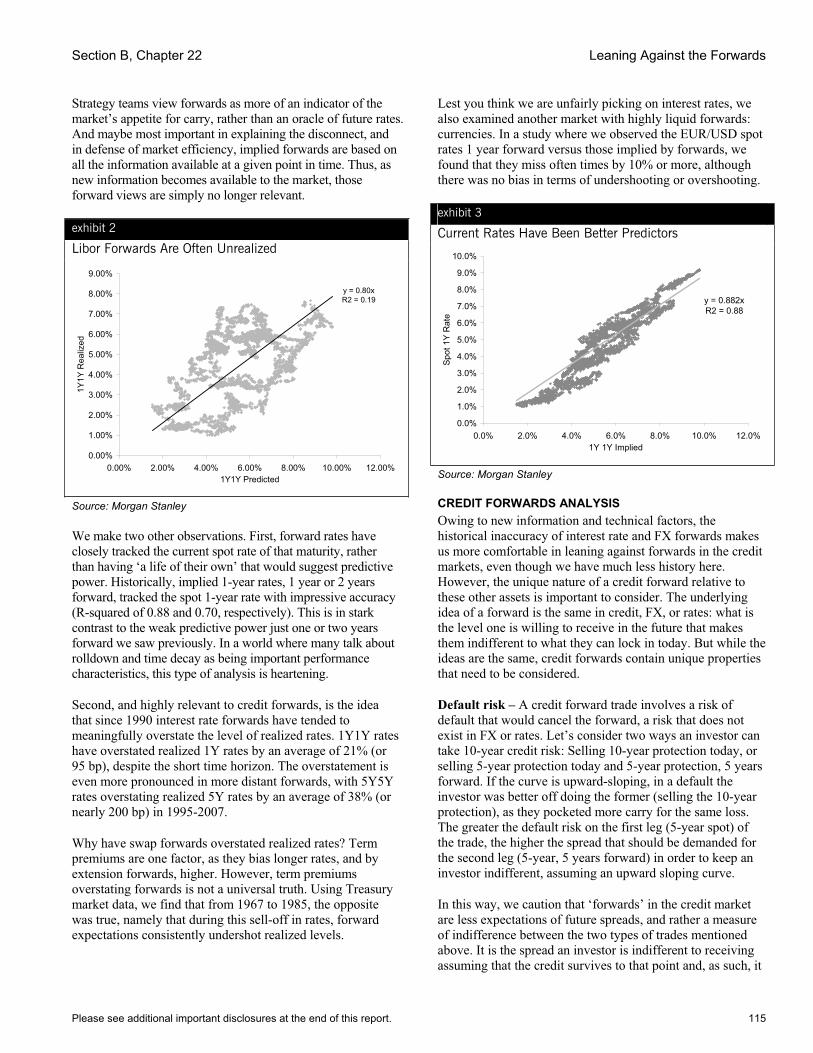
Section B, Chapter 22 Leaning Against the Forwards
Please see additional important disclosures at the end of this report. 115
Strategy teams view forwards as more of an indicator of the market’s appetite for carry, rather than an oracle of future rates. And maybe most important in explaining the disconnect, and in defense of market efficiency, implied forwards are based on all the information available at a given point in time. Thus, as new information becomes available to the market, those forward views are simply no longer relevant.
exhibit 2
Libor Forwards Are Often Unrealized
y = 0.80xR2 = 0.19
0.00%
1.00%
2.00%
3.00%
4.00%
5.00%
6.00%
7.00%
8.00%
9.00%
0.00% 2.00% 4.00% 6.00% 8.00% 10.00% 12.00%1Y1Y Predicted
1Y1Y
Rea
lized
Source: Morgan Stanley
We make two other observations. First, forward rates have closely tracked the current spot rate of that maturity, rather than having ‘a life of their own’ that would suggest predictive power. Historically, implied 1-year rates, 1 year or 2 years forward, tracked the spot 1-year rate with impressive accuracy (R-squared of 0.88 and 0.70, respectively). This is in stark contrast to the weak predictive power just one or two years forward we saw previously. In a world where many talk about rolldown and time decay as being important performance characteristics, this type of analysis is heartening.
Second, and highly relevant to credit forwards, is the idea that since 1990 interest rate forwards have tended to meaningfully overstate the level of realized rates. 1Y1Y rates have overstated realized 1Y rates by an average of 21% (or 95 bp), despite the short time horizon. The overstatement is even more pronounced in more distant forwards, with 5Y5Y rates overstating realized 5Y rates by an average of 38% (or nearly 200 bp) in 1995-2007.
Why have swap forwards overstated realized rates? Term premiums are one factor, as they bias longer rates, and by extension forwards, higher. However, term premiums overstating forwards is not a universal truth. Using Treasury market data, we find that from 1967 to 1985, the opposite was true, namely that during this sell-off in rates, forward expectations consistently undershot realized levels.
Lest you think we are unfairly picking on interest rates, we also examined another market with highly liquid forwards: currencies. In a study where we observed the EUR/USD spot rates 1 year forward versus those implied by forwards, we found that they miss often times by 10% or more, although there was no bias in terms of undershooting or overshooting.
exhibit 3
Current Rates Have Been Better Predictors
y = 0.882xR2 = 0.88
0.0%
1.0%
2.0%
3.0%
4.0%
5.0%
6.0%
7.0%
8.0%
9.0%
10.0%
0.0% 2.0% 4.0% 6.0% 8.0% 10.0% 12.0%1Y 1Y Implied
Spot
1Y
Rat
e
Source: Morgan Stanley
CREDIT FORWARDS ANALYSIS Owing to new information and technical factors, the historical inaccuracy of interest rate and FX forwards makes us more comfortable in leaning against forwards in the credit markets, even though we have much less history here. However, the unique nature of a credit forward relative to these other assets is important to consider. The underlying idea of a forward is the same in credit, FX, or rates: what is the level one is willing to receive in the future that makes them indifferent to what they can lock in today. But while the ideas are the same, credit forwards contain unique properties that need to be considered.
Default risk – A credit forward trade involves a risk of default that would cancel the forward, a risk that does not exist in FX or rates. Let’s consider two ways an investor can take 10-year credit risk: Selling 10-year protection today, or selling 5-year protection today and 5-year protection, 5 years forward. If the curve is upward-sloping, in a default the investor was better off doing the former (selling the 10-year protection), as they pocketed more carry for the same loss. The greater the default risk on the first leg (5-year spot) of the trade, the higher the spread that should be demanded for the second leg (5-year, 5 years forward) in order to keep an investor indifferent, assuming an upward sloping curve.
In this way, we caution that ‘forwards’ in the credit market are less expectations of future spreads, and rather a measure of indifference between the two types of trades mentioned above. It is the spread an investor is indifferent to receiving assuming that the credit survives to that point and, as such, it

Morgan Stanley Credit Derivatives Insights – Handbook of Single Name and Index Strategies
116 Please see additional important disclosures at the end of this report.
must compensate an investor for all the scenarios where it did not survive. It will therefore overstate the spread we would expect to see if we, say, held an option to invest 5 years forward, and could therefore check for survival. This overstatement will be very small at tighter spreads, but it increases with default risk and curve steepness.
Liquidity – Another factor affecting the ‘efficiency’ of forward trades is that liquidity issues can make the forwards harder to monetize. Long 7-year CDX 7, short 5-year CDX 7 is a long 2-year position, 5 years forward, constructed from two of the most liquid points on today’s curve. But 5 years forward, we will be on CDX 17, and the market for 2-year CDX 7 risk will likely suffer.
Ratings migration risk – When thinking about forward spreads in corporate credit, we note that any company can possibly look different several years down the road. A steep curve in an investment grade name could simply represent an expectation that the entity will be lower rated in five years time, rather than a mispricing.
Current CDX and iTraxx pricing suggest 1-5-year forward spreads that are much wider and flatter than we see today. Assuming for a moment that these levels accurately represent market expectations, they would at first glance suggest a much weaker macro credit environment, with wider and flatter curves. Flat investment grade credit curves have existed but are rare (1991, 2002). Such environments have been short-lived, and have generally coincided with market spreads greater than 100 bp and high default rates that have justified flat or inverted curves. This presents an interesting scenario to lean against. But how much of this ‘wider and flatter’ expectation is a weaker macro picture, and how much is credit deterioration over time?
To better understand the impact of credit deterioration over time, we show a pair of relationships in Exhibit 4 for generic A- rated credits versus the current iTraxx index (whose average rating is A-). The A- rated curve represents average agency expected losses over time for credits with this rating and is more or less a constant in CDO models. From this curve, we can compute a forward, which tells us what the steepness of the curve says about future losses, even these future losses are not implied because they are not derived from tradable instruments.
The relative differences of these agency loss curves and the market curves (for iTraxx) offer important insights, in our view, and show that the implied forward iTraxx curve is almost off the charts with respect to these other curves.
There is at least one flaw to this methodology, as it relies on the average deterioration of average ‘A-’ credit. As we have noted repeatedly in the past, credit losses and spreads are highly cyclical, so averages can be misleading. Several of our fellow strategists have noted a similarity between today’s
environment and 1996, and so we consider a 10-year cohort with iTraxx ratings formed in that year. This cohort saw 85% of its defaults in its back five years (2001-2006), and so we feel it is a fitting example, given the back-weighted defaults implied by current pricing.
exhibit 4
How Should Credit Deterioration Effect Forwards?
bp
0
10
20
30
40
50
60
70
1 2 3 4 5Years to Maturity
iTraxx 5 Yrs Fwd iTraxx SpotA- Loss Curve Fwd A- Loss Curve Spot
Source: Morgan Stanley Research, S&P, Moody’s
Using the same methodology as above, we find that with very few defaults between 1996-2000, the 5-year curve is understandably tight.
exhibit 5
Pricing a Back-Loaded Scenario – 1996 Perspective (bp)
0
10
20
30
40
50
60
70
1 2 3 4 5
iTraxx 5 Yrs Fwd iTraxx Spot1996 A- Loss Curve Fwd 1996 A- Loss Curve Spot
Source: Morgan Stanley Research, S&P, Moody’s
However, even under the heavily back-loaded losses of 2001-2006, spreads that would have compensated you for those losses are much, much lower than we currently observe in the iTraxx forwards. For the 1996 cohort, we see the curve 5 years forward invert, reflecting high defaults between 2000 and 2002. But after this spike, defaults crept back down, and ultimately dropped off sharply in 2004-2006. This suggests to us that iTraxx and CDX 5s10s are too steep based on

Section B, Chapter 22 Leaning Against the Forwards
Please see additional important disclosures at the end of this report. 117
historical losses, as 5Y5Y forwards are implying a scenario much worse than a back-loaded 2001-2002. But there are good arguments for curves to stay relatively steep.
CONCLUSION – IN WHICH DIRECTION DO WE LEAN? Going back to our initial theme, if one believes that the realization of credit forwards is only a rare event, and one has some intuition as to why they may not be realized, then there are trades to do. Here are some thoughts on products and strategies that are greatly influenced by the realization (or lack thereof) of forward credit spreads.
• Today’s duration-neutral steepeners in the single-name space are a reflection that the large amounts of positive carry and rolldown are so attractive that they serve as a self-fulfilling prophecy in keeping curves steep, even though forwards say they ought to flatten to make up for the carry. But taking the other side in tranches may make sense, as the absolute yield that longer-duration structured credit affords relative to shorter-duration instruments (because of term premium) is attractive to many types of market participants.
• Rolldown and time decay are concepts that have no place in a pure ‘no arbitrage’ world of forwards, but are key trade characteristics today, and if one believes that current rates/spreads are reasonable predictors of future levels, then they are important characteristics in general.
• CMCDS is an instrument that is priced directly from the forwards, and if one believes that forwards are too wide, then buying CMCDS protection makes sense to us, since the initially low premiums (in today’s steep curves) will not step up as much as implied by the forwards.
• Range accrual instruments in credit are quite new, but the concept of positioning for spreads to stay in a narrow range is in many ways taking an implicit view on forwards.
• Forwards are clearly central to the pricing of credit options, but since most option instruments are short-dated in nature, the forward component is less important. But embedded longer-dated ATM spot options in products like cancellable CDS and callable tranches may actually be more valuable (all else being equal), given that spreads may stay tighter (making refinancing more likely).
• CPDOs, in their current form, are trades that would perform poorly if forward credit spreads are realized. The agencies clearly do not take this into consideration in their ratings approaches, although perhaps they should. Regardless, long CPDO positions are ways of leaning against credit forwards; however, they can still significantly underperform for other reasons, given the leverage in the structures.

Morgan Stanley Credit Derivatives Insights – Handbook of Single Name and Index Strategies
118 Please see additional important disclosures at the end of this report.
Chapter 23
Credit Volatility – The Unintended Consequences April 1, 2005
Primary Analyst: Sivan Mahadevan Primary Analyst: Peter Polanskyj Primary Analyst: Ajit Kumar, CFA
Idiosyncratic events in the auto and media sectors, combined with a sharp jump into a new interest rate regime, have introduced a type of negative credit volatility that we have not seen in some time in the investment grade space. The credit-specific issues of a few have been impacting the market at large, and for the first time in a while, we have the opportunity to visualize the pricing impact of convexity in everything from a plain vanilla credit default swap to a first-loss tranche in a synthetic CDO.
When the big moves in spread that some welcome (or fear) actually are experienced, the realities of this convexity actually come to the forefront, however unintended they may be. The liquidity and standardization in today’s default swap market means that unwinding off-market swaps with standard par swaps can result in residual default risk, in the form of credit risky residual coupon streams, otherwise known as credit I/Os. This phenomenon can be even more exaggerated in index versus single-name positions, where credit default swaps are ‘fixed’ at inception at off-market levels, especially for credits that trade far away from index averages. Furthermore, we remind investors that the biggest impacts of sharp single-name moves are in the subordinate tranches of synthetic CDOs, and we explain some of the recent price movements on both an absolute basis and relative to what model deltas would have predicted.
SINGLE-NAME IMPLICATIONS: BUY/SELL VERSUS UNWINDConvexity is a well understood phenomenon in corporate bonds, both the convexity associated with large changes in interest rates or spreads and the changes in default risk for instruments that trade away from par, given that most bonds have a par claim in default. There is one significant difference between bonds and default swaps when it comes to credit convexity, namely the residual default risk resulting from unwinding positions. When an investor trades in and out of a specific bond, he or she is left with no residual risk, because the specific instrument that was initially bought (or sold) is subsequently sold (or bought). This may seem like an obvious statement, but it is important to understand that with default swaps, trading in and out of risk over time as swaps move ‘off-market’ can leave residual risks, depending on how the trades are actually performed.
Let’s consider the following example (see Exhibit 1), where an investor purchased 5-year protection on Delphi at 187 bp three months ago and then subsequently elected to ‘get out of the risk’ more recently at 516 bp. If the investor chose to simply sell protection at 516 bp (par swap) to the same date, then he/she would effectively earn the difference of 329 bp per annum (approximately $131,867 – $47,789 = $84,078 quarterly, assuming $10 million notional) until maturity, assuming both swaps were struck at prevailing market spreads when they traded. Since both contracts are still outstanding, there is still some residual risk to the investor in the event of an unexpected default, as the coupon stream would stop. In fact, if an immediate default occurred, the value of the missed coupon payments would be worth approximately $1.7 million, or 17% of the initial notional.
exhibit 1
Unwinding Delphi CDS – Two Scenarios
Original Contract
Off-Market Unwind
Scenario 1: Net Payments from Unwind
Unwind with New Par Swap
Scenario 2: Net Payments from an
Offsetting Par SwapContract Notional ($) 10,000,000 10,000,000 10,000,000Contract Strike (bp) 187 187 516Payments ($)
3/20/2005 1,212,929 1,212,929 6/20/2005 47,789 47,789 0 131,867 84,0789/20/2005 47,789 47,789 0 131,867 84,078
… … … … … …12/20/2009 47,269 47,269 0 130,433 83.164
3/20/2010 46,750 46,750 0 129,000 82,250
Residual Jump To Default Exposure ($ Undiscounted) 0 1,668,761
Source: Morgan Stanley
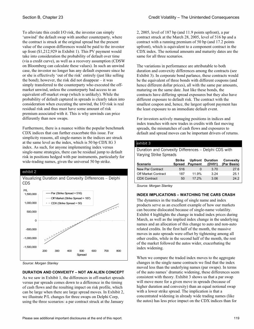
Section B, Chapter 23 Credit Volatility – The Unintended Consequences
Please see additional important disclosures at the end of this report. 119
To alleviate this credit I/O risk, the investor can simply ‘unwind’ the default swap with another counterparty, where the contract is struck at the original spread but the present value of the coupon differences would be paid to the investor up front ($1,212,929 in Exhibit 1). This PV payment would take into consideration the probability of default over time (via a credit curve), as well as a recovery assumption (CDSW on Bloomberg can calculate these values). In such an unwind case, the investor no longer has any default exposure since he or she is effectively ‘out of the risk’ entirely (just like selling the bond); however, the risk did not disappear – it was simply transferred to the counterparty who executed the off-market unwind, unless the counterparty had access to an equivalent off-market swap (which is unlikely). While the probability of default captured in spreads is clearly taken into consideration when executing the unwind, the I/O risk is real residual risk and thus must have some amount of risk premium associated with it. This is why unwinds can price differently than new swaps.
Furthermore, there is a nuance within the popular benchmark CDX indices that can further exacerbate this issue. For simplicity reasons, all single-names in the indices are struck at the same level as the index, which is 50 bp CDX IG 3 index. As such, for anyone implementing index versus single-name strategies, there can be residual jump to default risk in positions hedged with par instruments, particularly for wide-trading names, given the universal 50 bp strike.
exhibit 2
Visualizing Duration and Convexity Differences – Delphi CDS
P/L
-1,500,000
-1,000,000
-500,000
0
500,000
1,000,000
1,500,000
200 300 400 500 600 700 800Spread
Par (Strike Spread = 516)
Off Market (Strike Spread = 187)
CDX (Strike Spread = 50)
Source: Morgan Stanley
DURATION AND CONVEXITY – NOT AN ALIEN CONCEPT As we saw in Exhibit 1, the differences in off-market spreads versus par spreads comes down to a difference in the timing of cash flows and the resulting impact on risk profile, which can be large when there are large spread moves. In Exhibit 2, we illustrate P/L changes for three swaps on Delphi Corp, using the three scenarios: a par contract struck at the January
2, 2005, level of 187 bp (and 11.9 points upfront), a par contract struck at the March 28, 2005, level of 516 bp and a contract with a running premium of 50 bp (and 17.2 points upfront), which is equivalent to a component contract in the CDX index. The notional amounts and maturity dates are the same for all three scenarios.
The variations in performance are attributable to both duration and convexity differences among the contracts (see Exhibit 3). In corporate bond parlance, these contracts would be the equivalent of three bonds with different coupons (and hence different dollar prices), all with the same par amounts, maturing on the same date. Just like these bonds, the contracts have differing spread exposures but they also have different exposure to default risk. The contract with the smallest coupon and, hence, the largest upfront payment has the least exposure to an immediate default event.
For investors actively managing positions in indices and index tranches with new trades in credits with fast moving spreads, the mismatches of cash flows and exposures to default and spread moves can be important drivers of returns.
exhibit 3
Duration and Convexity Differences – Delphi CDS with Varying Strike Spreads
ScenarioStrike
SpreadUpfront
Payment Duration
(DV01)Convexity
(Par Basis)New Par Contract 516 0 3.70 27.6Off Market Contract 187 11.9% 3.24 25.1CDX Contract 50 17.2% 3.06 24.2
Source: Morgan Stanley
INDEX IMPLICATIONS – WATCHING THE CARS CRASH The dynamics in the trading of single name and index products serve as an excellent example of how our markets can become dislocated because of single-name volatility. Exhibit 4 highlights the change in traded index prices during March, as well as the implied index change in the underlying names and an allocation of this change to auto and non-auto related credits. In the first half of the month, the massive moves in auto spreads were offset by tightening among all other credits, while in the second half of the month, the rest of the market followed the autos wider, exacerbating the index widening.
When we compare the traded index moves to the aggregate changes in the single name contracts we find that the index moved less than the underlying names (par swaps). In terms of the auto names’ dramatic widening, these differences seem consistent with theory. Exhibit 3 shows us that a par swap will move more for a given move in spreads (because of higher duration and convexity) than an equal notional swap with a lower strike spread. The implication is that a concentrated widening in already wide trading names (like the autos) has less price impact on the CDX indices than for
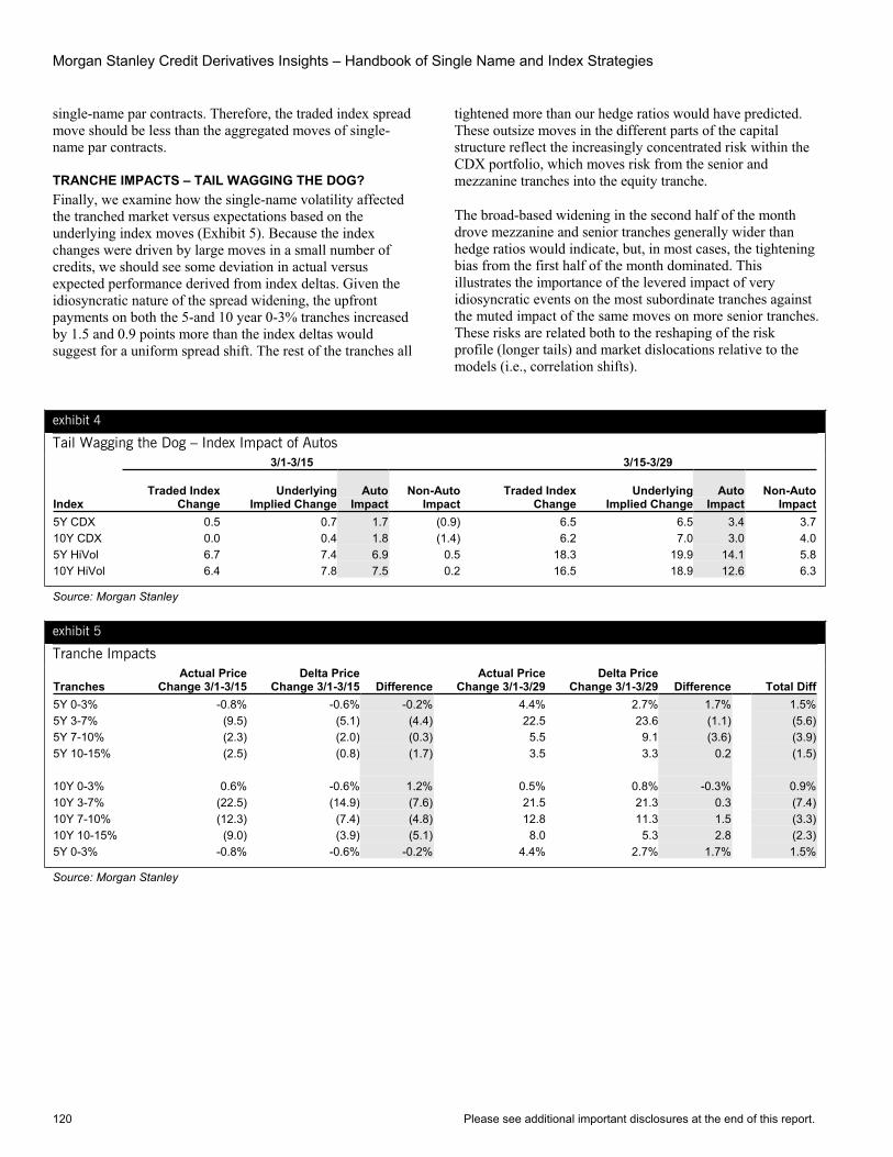
Morgan Stanley Credit Derivatives Insights – Handbook of Single Name and Index Strategies
120 Please see additional important disclosures at the end of this report.
single-name par contracts. Therefore, the traded index spread move should be less than the aggregated moves of single-name par contracts.
TRANCHE IMPACTS – TAIL WAGGING THE DOG? Finally, we examine how the single-name volatility affected the tranched market versus expectations based on the underlying index moves (Exhibit 5). Because the index changes were driven by large moves in a small number of credits, we should see some deviation in actual versus expected performance derived from index deltas. Given the idiosyncratic nature of the spread widening, the upfront payments on both the 5-and 10 year 0-3% tranches increased by 1.5 and 0.9 points more than the index deltas would suggest for a uniform spread shift. The rest of the tranches all
tightened more than our hedge ratios would have predicted. These outsize moves in the different parts of the capital structure reflect the increasingly concentrated risk within the CDX portfolio, which moves risk from the senior and mezzanine tranches into the equity tranche.
The broad-based widening in the second half of the month drove mezzanine and senior tranches generally wider than hedge ratios would indicate, but, in most cases, the tightening bias from the first half of the month dominated. This illustrates the importance of the levered impact of very idiosyncratic events on the most subordinate tranches against the muted impact of the same moves on more senior tranches. These risks are related both to the reshaping of the risk profile (longer tails) and market dislocations relative to the models (i.e., correlation shifts).
exhibit 4
Tail Wagging the Dog – Index Impact of Autos 3/1-3/15 3/15-3/29
IndexTraded Index
Change Underlying
Implied Change Auto
ImpactNon-Auto
ImpactTraded Index
ChangeUnderlying
Implied Change Auto
ImpactNon-Auto
Impact5Y CDX 0.5 0.7 1.7 (0.9) 6.5 6.5 3.4 3.710Y CDX 0.0 0.4 1.8 (1.4) 6.2 7.0 3.0 4.05Y HiVol 6.7 7.4 6.9 0.5 18.3 19.9 14.1 5.810Y HiVol 6.4 7.8 7.5 0.2 16.5 18.9 12.6 6.3
Source: Morgan Stanley
exhibit 5
Tranche Impacts
Tranches Actual Price
Change 3/1-3/15 Delta Price
Change 3/1-3/15 DifferenceActual Price
Change 3/1-3/29Delta Price
Change 3/1-3/29 Difference Total Diff5Y 0-3% -0.8% -0.6% -0.2% 4.4% 2.7% 1.7% 1.5%5Y 3-7% (9.5) (5.1) (4.4) 22.5 23.6 (1.1) (5.6)5Y 7-10% (2.3) (2.0) (0.3) 5.5 9.1 (3.6) (3.9)5Y 10-15% (2.5) (0.8) (1.7) 3.5 3.3 0.2 (1.5) 10Y 0-3% 0.6% -0.6% 1.2% 0.5% 0.8% -0.3% 0.9%10Y 3-7% (22.5) (14.9) (7.6) 21.5 21.3 0.3 (7.4)10Y 7-10% (12.3) (7.4) (4.8) 12.8 11.3 1.5 (3.3)10Y 10-15% (9.0) (3.9) (5.1) 8.0 5.3 2.8 (2.3)5Y 0-3% -0.8% -0.6% -0.2% 4.4% 2.7% 1.7% 1.5%
Source: Morgan Stanley

Please see additional important disclosures at the end of this report. 121
Chapter 24
Volatility Confuses Credit Spreads June 3, 2005
Primary Analyst: Sivan Mahadevan Primary Analyst: Peter Polanskyj Primary Analyst: Ajit Kumar, CFA
There are many aspects of credit markets that we find confusing today. While it is easy to dismiss market activity as being technical in nature given both dealer and hedge fund activity, such a sentiment is not very helpful for investors attempting to position credit portfolios going forward. When technicals dominate, looking for answers in other markets can sometimes be helpful, but there can be technical issues there as well.
We have been fans of at least garnering indications of default risk and credit valuation from the equity markets through equity volatility, Merton models and the like. While equity volatility and credit spreads have been directionally consistent since volatility itself kicked up nearly 3 months ago, changes in equity volatility (both realized and implied) have been far more muted than changes in credit spreads, in both directions. Using a Merton framework, credit at today’s wider spread levels looks the cheapest it has been since we started tracking the relationship in 2001, for both investment grade and high yield issuers. Furthermore, if we simply focus on the equity volatility and credit spread relationship, we can easily observe the differences in magnitude of the shifts, particularly in sectors where credit investors fear capital structure changes.
However, we caution that volatility implied from the equity options markets can be misleading in this environment, as technical factors related to structured equity products have been keeping implied volatility low. As such, when we compare implied with historical volatility, we find some interesting differences, particularly in the auto, energy and financial sectors.
MERTON MODELS VS. SPREADS – CREDIT MARKETS IMPLY MUCH MORE DEFAULT RISK In a Merton context, we have found the relationship of default risk measured by both markets (equity via KMV EDFs and credit via default swap levels) to be an interesting relative value measure. Credit markets will generally imply more default risk because of risk premium in credit spreads, but the ratio of the two has never been higher since we first started tracking it at the end of 2001 (see Exhibit 1 for both investment grade and high yield). Muted shifts in equity volatility (realized instead of implied for KMV EDFs), nearly unchanged stock prices (the S&P 500 is flat since the end of February) and still very healthy corporate leverage levels are the main reasons why EDFs continue to stay low despite wider spreads.
exhibit 1
Credit Markets Imply More Default Risk– Ratio of Spread-Implied Default Rates and EDFs
Spread Implied Def Rate / EDF
0
2
4
6
8
10
12
Dec-01 Sep-02 May-03 Jan-04 Sep-04 May-05
Investment Grade
High Yield
Source: Morgan Stanley, Moody’s KMV
If we dig a little deeper into the analysis, we find that the rise in credit market implied default risk relative to EDFs is actually only partially driven by the wider trading names in the investment grade space. Credits in the 40 to 60 bp zipcode are the biggest drivers of the change, as low leverage levels and low equity volatility have pushed EDFs to near zero levels. Our universe is comprised of 160 investment grade names and another 160 high yield names, although for the latter, the universe was much smaller historically. We compare one-year EDFs with five-year CDS levels, which does have some curve risk in it, but we find that five-year EDFs show similarly-shaped results.
VOLATILITY VS. CREDIT SPREADS – A SIMPLER APPROACH For those who might be skeptical of complicated credit models like KMV, one can examine equity volatility and credit spread relationships using a much more simple approach. We find that although credit spreads today (CDS levels) are well off their wides from two weeks ago, they have indeed widened more than implied equity volatility has risen, when compared on an apples-to-apples basis (see Exhibit 2). In fact, the magnitude shift in this relationship is the largest it has been since we started tracking it in 2002.
To make comparisons legitimate, we normalize the data by using historical Z-Scores, which is the number of standard deviations away from the mean (we track these values at the credit specific level regularly in our weekly CreditDerivatives Insights publication). Our universe includes 185 largely investment grade credits. Note that implied equity volatility is for a 2-month maturity at-the-money put option.
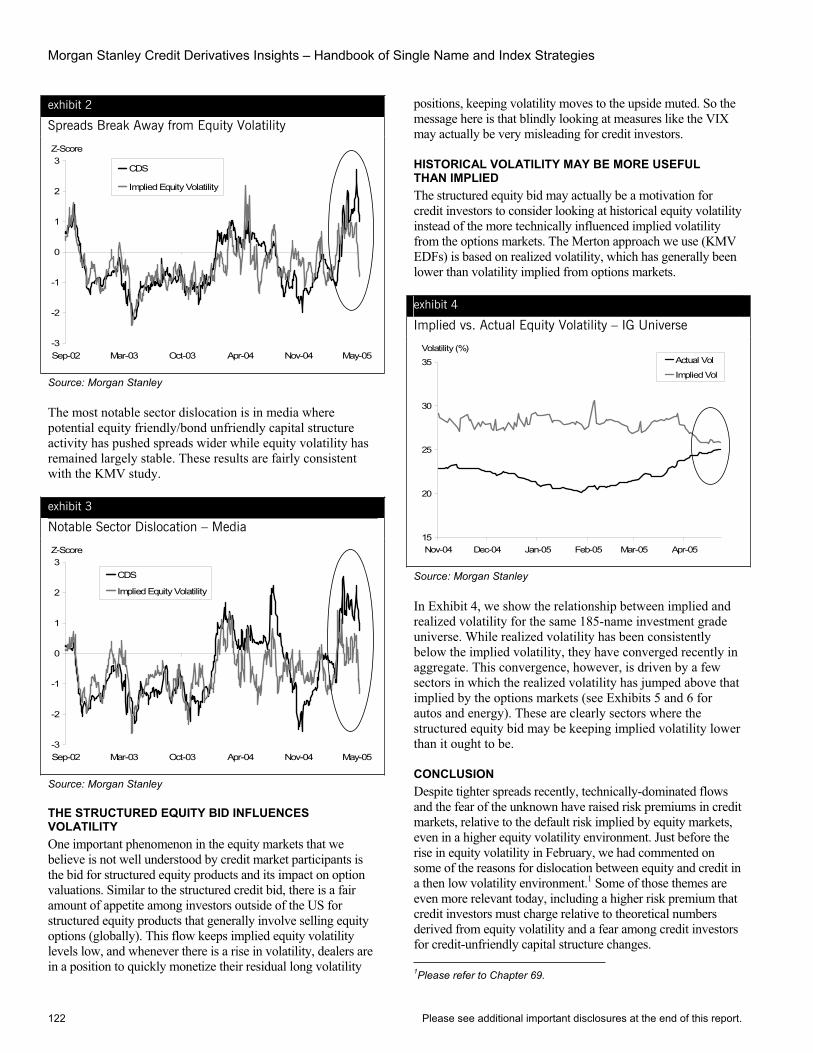
Morgan Stanley Credit Derivatives Insights – Handbook of Single Name and Index Strategies
122 Please see additional important disclosures at the end of this report.
exhibit 2
Spreads Break Away from Equity Volatility
Z-Score
-3
-2
-1
0
1
2
3
Sep-02 Mar-03 Oct-03 Apr-04 Nov-04 May-05
CDS
Implied Equity Volatility
Source: Morgan Stanley
The most notable sector dislocation is in media where potential equity friendly/bond unfriendly capital structure activity has pushed spreads wider while equity volatility has remained largely stable. These results are fairly consistent with the KMV study.
exhibit 3
Notable Sector Dislocation – Media
Z-Score
-3
-2
-1
0
1
2
3
Sep-02 Mar-03 Oct-03 Apr-04 Nov-04 May-05
CDS
Implied Equity Volatility
Source: Morgan Stanley
THE STRUCTURED EQUITY BID INFLUENCES VOLATILITY One important phenomenon in the equity markets that we believe is not well understood by credit market participants is the bid for structured equity products and its impact on option valuations. Similar to the structured credit bid, there is a fair amount of appetite among investors outside of the US for structured equity products that generally involve selling equity options (globally). This flow keeps implied equity volatility levels low, and whenever there is a rise in volatility, dealers are in a position to quickly monetize their residual long volatility
positions, keeping volatility moves to the upside muted. So the message here is that blindly looking at measures like the VIX may actually be very misleading for credit investors.
HISTORICAL VOLATILITY MAY BE MORE USEFUL THAN IMPLIED The structured equity bid may actually be a motivation for credit investors to consider looking at historical equity volatility instead of the more technically influenced implied volatility from the options markets. The Merton approach we use (KMV EDFs) is based on realized volatility, which has generally been lower than volatility implied from options markets.
exhibit 4
Implied vs. Actual Equity Volatility – IG Universe
Volatility (%)
15
20
25
30
35
Nov-04 Dec-04 Jan-05 Feb-05 Mar-05 Apr-05
Actual Vol
Implied Vol
Source: Morgan Stanley
In Exhibit 4, we show the relationship between implied and realized volatility for the same 185-name investment grade universe. While realized volatility has been consistently below the implied volatility, they have converged recently in aggregate. This convergence, however, is driven by a few sectors in which the realized volatility has jumped above that implied by the options markets (see Exhibits 5 and 6 for autos and energy). These are clearly sectors where the structured equity bid may be keeping implied volatility lower than it ought to be.
CONCLUSIONDespite tighter spreads recently, technically-dominated flows and the fear of the unknown have raised risk premiums in credit markets, relative to the default risk implied by equity markets, even in a higher equity volatility environment. Just before the rise in equity volatility in February, we had commented on some of the reasons for dislocation between equity and credit in a then low volatility environment.1 Some of those themes are even more relevant today, including a higher risk premium that credit investors must charge relative to theoretical numbers derived from equity volatility and a fear among credit investors for credit-unfriendly capital structure changes. 1Please refer to Chapter 69.
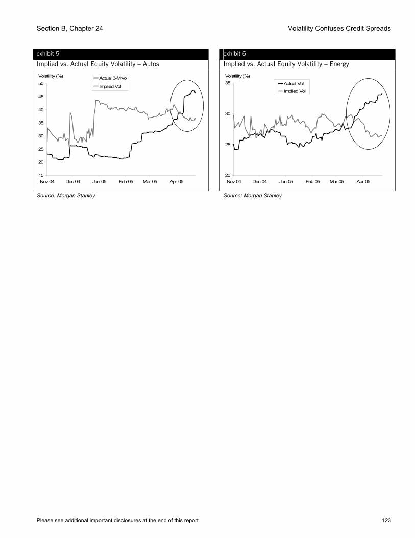
Section B, Chapter 24 Volatility Confuses Credit Spreads
Please see additional important disclosures at the end of this report. 123
exhibit 5
Implied vs. Actual Equity Volatility – Autos
Volatility (%)
15
20
25
30
35
40
45
50
Nov-04 Dec-04 Jan-05 Feb-05 Mar-05 Apr-05
Actual 3-M vol
Implied Vol
Source: Morgan Stanley
exhibit 6
Implied vs. Actual Equity Volatility – Energy
Volatility (%)
20
25
30
35
Nov-04 Dec-04 Jan-05 Feb-05 Mar-05 Apr-05
Actual Vol
Implied Vol
Source: Morgan Stanley
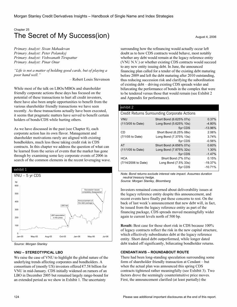
Morgan Stanley Credit Derivatives Insights – Handbook of Single Name and Index Strategies
124 Please see additional important disclosures at the end of this report.
Chapter 25
The Secret of My Success(ion) August 4, 2006
Primary Analyst: Sivan Mahadevan Primary Analyst: Peter Polanskyj Primary Analyst: Vishwanath Tirupattur Primary Analyst: Pinar Onur
“Life is not a matter of holding good cards, but of playing a poor hand well.”
– Robert Louis Stevenson
While most of the talk on LBOs/MBOs and shareholder friendly corporate actions these days has focused on the potential of these transactions to hurt all credit investors, there have also been ample opportunities to benefit from the various shareholder friendly transactions we have seen recently. As these transactions actually have been executed, it seems that pragmatic matters have served to benefit certain holders of bonds/CDS while hurting others.
As we have discussed in the past (see Chapter 8), each corporate action has its own flavor. Management and shareholder motivations rarely are aligned with existing bondholders, much less those taking credit risk in CDS contracts. In this chapter we address the question of what can be learned from the series of events that the market has gone through by examining some key corporate events of 2006 in search of the common elements in the recent leveraging wave.
exhibit 1
VNU – 5 yr CDS
0
100
200
300
400
500
600
Jan-05 May-05 Aug-05 Oct-05 Jan-06 May-06 Jul-06
bp
Succession issues completely disappeared
Announcement of the debt package
LBO speculation in the press
LBO bid
Source: Morgan Stanley
VNU – STEREOTYPICAL LBO We raise the case of VNU to highlight the global nature of the underlying trends affecting corporates and bondholders. A consortium of (mostly US) investors offered €7.58 billion for VNU in mid-January. CDS initially widened on rumors of an LBO in December 2005 but remained largely range-bound for an extended period as we show in Exhibit 1. The uncertainty
surrounding how the refinancing would actually occur left doubt as to how CDS contracts would behave, most notably whether any debt would remain at the legacy reference entity (VNU N.V.) or whether existing CDS contracts would succeed to any new entity issuing debt. In June, the announced financing plan called for a tender of the existing debt maturing before 2009 and left the debt maturing after 2010 outstanding, thus reducing succession risk and clarifying the subordination of existing debt – driving existing CDS spreads wider and bifurcating the performance of bonds in the complex that were to be tendered versus those that would remain (see Exhibit 2 and Appendix for performance).
exhibit 2
Credit Returns Surrounding Corporate Actions VNU Short Bond (6.625% 07s) 0.37%(11/3/05 to Date) Long Bond (5.625% 10s) -4.80%
5yr CDS -13.96%CD Short Bond (6.25% 08s) 2.06%(7/1/05 to Date) Long Bond (7.375% 13s) 3.74% 5yr CDS -0.56%AT Short Bond (4.656% 07s) 0.60%(11/1/05 to Date) Long Bond (7.875% 32s) 1.30%
5yr CDS -1.47%HCA Short Bond (7% 07s) 0.15%(7/14/2006 to Date) Long Bond (7.5% 33s) -19.37% 5yr CDS -10.71%
Note: Bond returns exclude interest rate impact. Assumes duration neutral treasury hedge.
Source: Morgan Stanley, Bloomberg
Investors remained concerned about deliverability issues at the legacy reference entity despite this announcement, and recent events have finally put these concerns to rest. On the back of last week’s announcement that new debt will, in fact, be issued from the legacy reference entity as part of the financing package, CDS spreads moved meaningfully wider again to current levels north of 500 bp.
Result: Best case for those short risk in CDS because 100% of legacy contracts reflect the risk in the new capital structure, which effectively subordinates debt at the legacy reference entity. Short dated debt outperformed, while longer dated debt traded off significantly, bifurcating bondholder returns.
CENDANT/AVIS – ROUNDABOUT ROUTE There had been long-standing speculation surrounding some form of shareholder friendly transaction at Cendant – but when the actual plan was announced this spring CDS contracts tightened rather meaningfully (see Exhibit 3). Two factors drove the seemingly counterintuitive price moves. First, the announcement clarified (at least partially) the

Section B, Chapter 25 The Secret of My Success(ion)
Please see additional important disclosures at the end of this report. 125
mechanics of the plan to divide the company into its various segments. This brought to the forefront the possibility that existing Cendant CDS contracts may not succeed to any of the new entities, while the legacy reference entity retained virtually no debt because the company planned to largely pay the existing debt down in a manner that would not trigger succession language. Second, the well-established short base in the name created a technical environment that could exacerbate the tightening.
exhibit 3
CD and JNY – Spreads Can Be Very Jumpy
0
50
100
150
200
250
Aug-05 Oct-05 Dec-05 Mar-06 May-06 Jul-06
CDJNY
Source: Morgan Stanley, Bloomberg
Interestingly, actual holders of Cendant debt fared well as most of the debt at the Cendant level was tendered for and Cendant protection continued to trade in the 50-60 bp range. Recently this rather sanguine view of the risk at Cendant may have changed as the market has come to appreciate that the old Cendant reference entity is essentially a holding company for the Avis business, which is subordinated to any newly issued debt at Avis, yet Cendant CDS trades well inside Avis debt and CDS levels (just north of 200 bp). The change in perception has driven Cendant CDS from around 50 to the 90-100 range (Exhibit 3) in a very short period.
Result: Most existing Cendant bondholders benefited from tender; CDS spreads remain 45 basis points tighter than preannouncement levels after recent widening (see Exhibit 2 and the Appendix for performance).
TELECOM SECTOR – MERGER MANIA TO SPIN-OFF SPRINTThe telecom space has been through a rather dramatic shift in the last several years, not just in terms of business model but also in terms of the industry theme of consolidation that was dominant over the last several years, moving to the theme of monetizing balance sheet assets we are seeing today. Several years ago we were recommending structured credit trades to investors who wanted to play the consolidation theme (see Credit Derivative Insights, “Trekking the TMT Terrain,”
December 5, 2003). Today, the opposite theme has clearly taken hold with various companies looking to extract value from balance sheet assets.
Alltel, Sprint Nextel and Verizon are the recent (and current) examples of this trend and highlight how the structure of deals can be driven by considerations like taxes while at the same time directly affecting bond and CDS holders. A common theme among the recent telecom corporate events is that the assets identified for monetization are likely to have relatively low tax bases and are generally underleveraged.
Using Alltel as an example, the company essentially swapped existing debt for new debt issued by the new wireline entity, driven by tax efficiency and a desire to leverage the wireline entity. Because the swap was “in conjunction with” the event, it generally triggered succession language under CDS contracts. This resulted in the effective split of legacy contracts into two: one referring to the original legacy company and one referring to the new wireline company. While the transaction was credit-enhancing for the original entity, the new entity is more highly levered and the weighted average impact was a widening of CDS spreads, although muted because only a portion of the original contract notional succeeds to the entity that actually trades wider (see Exhibit 2 for performance).
Result: Very short end bondholders benefited from tenders. Longer dated bondholders benefited from perceived credit enhancement, and being short risk in CDS worked out as well but the price impact was muted by the succession contract split.
LOOKING FORWARD The LBO/MBO and M&A environment continues to be hot, and the credit market seems hyper-sensitive to this trend – but only to the extent that it affects specific names, as the broader market has remained largely unaffected. As those who were involved in VNU learned, credit spreads can move early but clarity on the actual transaction terms is required for the market to fully price in the risk. As an example, the Jones NY CDS spread moved wider by 100 bp in late March (see Exhibit 3) on the back of news of a potential sale of the company but has been range-bound since, given uncertainty related to any transaction.
HCA appears to be developing in a manner similar to VNU, although it is a much bigger transaction with a much more severe bifurcation in cash performance: We have seen shorter dated bonds outperforming and longer dated bonds trading off significantly after the announcement that most of the short dated debt would be “tendered or repaid” (see Exhibit 2 for performance). CDS contracts widened markedly given the majority of existing debt seems likely to remain at the legacy reference entity, which looks to be subordinated to the new financing.
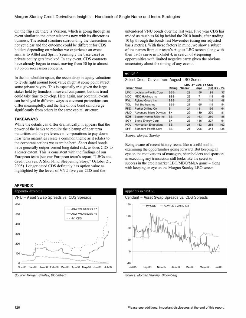
Morgan Stanley Credit Derivatives Insights – Handbook of Single Name and Index Strategies
126 Please see additional important disclosures at the end of this report.
On the flip side there is Verizon, which is going through an event similar to the other telecoms now with its directories business. The actual structure surrounding the transaction is not yet clear and the outcome could be different for CDS holders depending on whether we experience an event similar to Alltel and Sprint (seemingly the base case) or private equity gets involved. In any event, CDS contracts have already begun to react, moving from 30 bp to almost 80 bp on succession concerns.
In the homebuilder space, the recent drop in equity valuations to levels right around book value might at some point attract some private buyers. This is especially true given the large stakes held by founders in several companies, but this trend could take time to develop. Here again, any potential events can be played in different ways as covenant protections can differ meaningfully, and the fate of one bond can diverge significantly from others in the same capital structure.
TAKEAWAYS While the details can differ dramatically, it appears that the power of the banks to require the cleanup of near term maturities and the preference of corporations to pay down near term maturities create a common theme as it relates to the corporate actions we examine here. Short dated bonds have generally outperformed long dated risk, as does CDS to a lesser extent. This is consistent with the findings of our European team (see our European team’s report, “LBOs and Credit Curves: A Short-End Steepening Story,” October 21, 2005). Longer dated CDS definitely has option value as highlighted by the levels of VNU five year CDS and the
untendered VNU bonds over the last year. Five year CDS has traded as much as 86 bp behind the 2010 bonds, after trading 10 bp through the bonds last November (using our adjusted basis metric). With these factors in mind, we show a subset of the names from our team’s August LBO screen along with their 3s-5s curve in Exhibit 4, in search of steepening opportunities with limited negative carry given the obvious uncertainty about the timing of any events.
exhibit 4
Select Credit Curves from August LBO Screen
Ticker Name Rating LBO
“Score” 3Y CDS
(bp)5Y CDS
(bp) 3’s - 5'sLPX Louisiana-Pacific Corp BBB- 22 56 93 37MDC MDC Holdings Inc BBB- 22 71 119 48RYL Ryland Group Inc BBB- 22 71 119 48TOL Toll Brothers Inc BBB- 21 65 119 54PKD Parker Drilling Co B 24 131 195 64AMD Advanced Micro Devices B+ 22 189 270 81BZH Beazer Homes USA Inc BB 22 163 250 88SGY Stone Energy Corp B+ 23 136 227 91HOV Hovnanian Enterprises BB 21 153 255 102SPF Standard-Pacific Corp BB 21 206 344 138
Source: Morgan Stanley
Being aware of recent history seems like a useful tool in examining the opportunities going forward. But keeping an eye on the motivations of managers, shareholders and sponsors in executing any transaction still looks like the secret to success in the credit market LBO/MBO/M&A game – along with keeping an eye on the Morgan Stanley LBO screen.
APPENDIX appendix exhibit 1
VNU – Asset Swap Spreads vs. CDS Spreads
0
100
200
300
400
500
600
Nov-05 Dec-05 Jan-06 Feb-06 Mar-06 Apr-06 May-06 Jun-06 Jul-06
ASW VNU 6.625% 07
ASW VNU 5.625% 10
5Yr CDS
Source: Morgan Stanley, Bloomberg
appendix exhibit 2
Cendant – Asset Swap Spreads vs. CDS Spreads
-40
0
40
80
120
160
Jul-05 Sep-05 Nov-05 Jan-06 Mar-06 May-06 Jul-06
5yr CDS ASW CD 7.375% 13s
Source: Morgan Stanley, Bloomberg
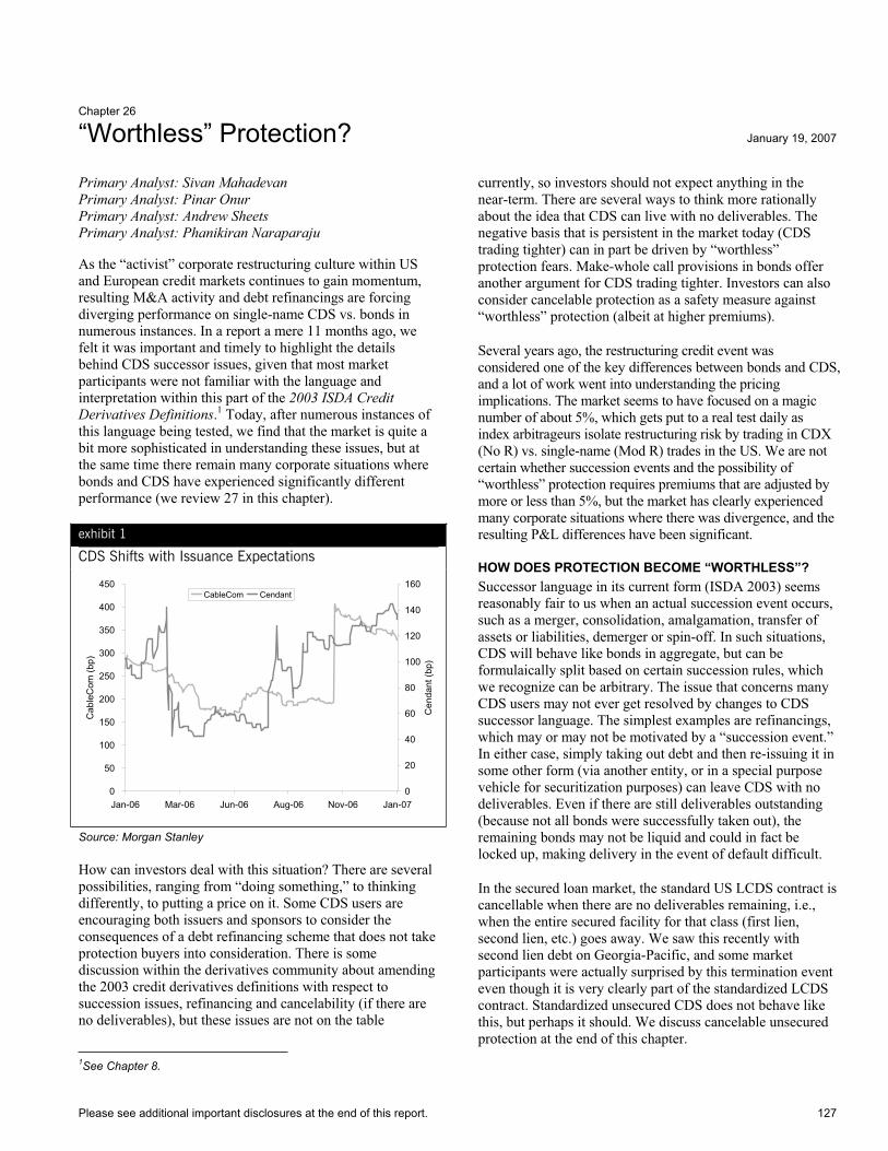
Please see additional important disclosures at the end of this report. 127
Chapter 26
“Worthless” Protection? January 19, 2007
Primary Analyst: Sivan Mahadevan Primary Analyst: Pinar Onur Primary Analyst: Andrew Sheets Primary Analyst: Phanikiran Naraparaju
As the “activist” corporate restructuring culture within US and European credit markets continues to gain momentum, resulting M&A activity and debt refinancings are forcing diverging performance on single-name CDS vs. bonds in numerous instances. In a report a mere 11 months ago, we felt it was important and timely to highlight the details behind CDS successor issues, given that most market participants were not familiar with the language and interpretation within this part of the 2003 ISDA Credit Derivatives Definitions.1 Today, after numerous instances of this language being tested, we find that the market is quite a bit more sophisticated in understanding these issues, but at the same time there remain many corporate situations where bonds and CDS have experienced significantly different performance (we review 27 in this chapter).
exhibit 1
CDS Shifts with Issuance Expectations
0
50
100
150
200
250
300
350
400
450
Jan-06 Mar-06 Jun-06 Aug-06 Nov-06 Jan-07
Cab
leC
om (b
p)
0
20
40
60
80
100
120
140
160
Cen
dant
(bp)
CableCom Cendant
Source: Morgan Stanley
How can investors deal with this situation? There are several possibilities, ranging from “doing something,” to thinking differently, to putting a price on it. Some CDS users are encouraging both issuers and sponsors to consider the consequences of a debt refinancing scheme that does not take protection buyers into consideration. There is some discussion within the derivatives community about amending the 2003 credit derivatives definitions with respect to succession issues, refinancing and cancelability (if there are no deliverables), but these issues are not on the table
1See Chapter 8.
currently, so investors should not expect anything in the near-term. There are several ways to think more rationally about the idea that CDS can live with no deliverables. The negative basis that is persistent in the market today (CDS trading tighter) can in part be driven by “worthless” protection fears. Make-whole call provisions in bonds offer another argument for CDS trading tighter. Investors can also consider cancelable protection as a safety measure against “worthless” protection (albeit at higher premiums).
Several years ago, the restructuring credit event was considered one of the key differences between bonds and CDS, and a lot of work went into understanding the pricing implications. The market seems to have focused on a magic number of about 5%, which gets put to a real test daily as index arbitrageurs isolate restructuring risk by trading in CDX (No R) vs. single-name (Mod R) trades in the US. We are not certain whether succession events and the possibility of “worthless” protection requires premiums that are adjusted by more or less than 5%, but the market has clearly experienced many corporate situations where there was divergence, and the resulting P&L differences have been significant.
HOW DOES PROTECTION BECOME “WORTHLESS”? Successor language in its current form (ISDA 2003) seems reasonably fair to us when an actual succession event occurs, such as a merger, consolidation, amalgamation, transfer of assets or liabilities, demerger or spin-off. In such situations, CDS will behave like bonds in aggregate, but can be formulaically split based on certain succession rules, which we recognize can be arbitrary. The issue that concerns many CDS users may not ever get resolved by changes to CDS successor language. The simplest examples are refinancings, which may or may not be motivated by a “succession event.” In either case, simply taking out debt and then re-issuing it in some other form (via another entity, or in a special purpose vehicle for securitization purposes) can leave CDS with no deliverables. Even if there are still deliverables outstanding (because not all bonds were successfully taken out), the remaining bonds may not be liquid and could in fact be locked up, making delivery in the event of default difficult.
In the secured loan market, the standard US LCDS contract is cancellable when there are no deliverables remaining, i.e., when the entire secured facility for that class (first lien, second lien, etc.) goes away. We saw this recently with second lien debt on Georgia-Pacific, and some market participants were actually surprised by this termination event even though it is very clearly part of the standardized LCDS contract. Standardized unsecured CDS does not behave like this, but perhaps it should. We discuss cancelable unsecured protection at the end of this chapter.
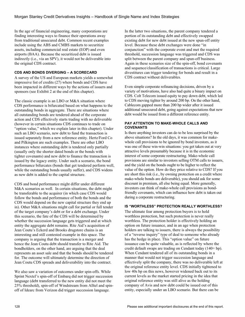
Morgan Stanley Credit Derivatives Insights – Handbook of Single Name and Index Strategies
128 Please see additional important disclosures at the end of this report.
In the age of financial engineering, many corporations are finding interesting ways to finance their operations away from traditional unsecured debt. Common recent examples include using the ABS and CMBS markets to securitize assets, including commercial real estate (EOP) and even airports (BAA). Because the securitized debt is issued indirectly (i.e., via an SPV), it would not be deliverable into the original CDS contract.
CDS AND BONDS DIVERGING – A SCORECARD A survey of the US and European markets yields a somewhat impressive list of credits (27) where bonds and CDS have been impacted in different ways by the actions of issuers and sponsors (see Exhibit 2 at the end of this chapter).
The classic example is an LBO or M&A situation where CDS performance is bifurcated based on what happens to the outstanding bonds in aggregate. There are situations where all outstanding bonds are tendered ahead of the corporate action and CDS effectively starts trading with no deliverable (however in certain situations CDS continues to trade on “option value,” which we explain later in this chapter). Under such an LBO scenario, new debt to fund the transaction is issued separately from a new reference entity. Hertz/Ford Co and Pilkington are such examples. There are other LBO instances where outstanding debt is tendered only partially (usually only the shorter dated bonds or the bonds with tighter covenants) and new debt to finance the transaction is issued by the legacy entity. Under such a scenario, the bond performance bifurcates (bonds that get tendered perform well, while the outstanding bonds usually suffer), and CDS widens as new debt is added to the capital structure.
CDS and bond performance might differ under different M&A scenarios as well. In certain situations, the debt might be transferable to the acquirer (in which case CDS would follow the bonds and performance of both the bonds and the CDS would depend on the new capital structure they end up in). Other M&A situations might call for partial or full tender of the target company’s debt or for a debt exchange. Under this scenario, the fate of the CDS will be determined by whether the succession language gets triggered and at which entity the aggregate debt remains. Rite Aid’s acquisition of Jean Coutu’s Eckerd and Brooks drugstore chains is an interesting and still contested example in this space. The company is arguing that the transaction is a merger and hence the Jean Coutu debt should transfer to Rite Aid. The bondholders, on the other hand, are arguing that the deal represents an asset sale and that the bonds should be tendered for. The outcome will ultimately determine the direction of Jean Coutu CDS spreads and deliverability into the contract.
We also saw a variation of outcomes under spin-offs. While Sprint Nextel’s spin-off of Embarq did not trigger succession language (debt transferred to the new entity did not meet the 25% threshold), spin-off of Windstream from Alltel and spin-off of Idearc from Verizon did trigger succession language.
In the latter two situations, the parent company tendered a portion of its outstanding debt and effectively swapped existing debt for new debt issued at the new spun-off entity level. Because these debt exchanges were done “in conjunction” with the corporate event and met the required threshold, succession language was triggered and CDS was split between the parent company and spun-off business. Again in these scenarios size of the spin-off, bond covenants and sequence/classification of transactions is critical. Large divestitures can trigger tendering for bonds and result in a CDS contract without deliverables.
Even simple corporate refinancing decisions, driven by a variety of motivations, have also had quite a binary impact on CDS. Colt Telecom issued equity to pay down debt, which led to CDS moving tighter by around 200 bp. On the other hand, Cablecom gapped more than 200 bp wider after it issued additional unsecured debt, going against expectations that new debt would be issued from a different reference entity.
PAY ATTENTION TO MAKE-WHOLE CALLS AND COVENANTS Is there anything investors can do to be less surprised by the above situations? In the old days, it was common for make-whole call provisions to be ignored by bond investors, as it was one of these win-win situations: you get taken out at very attractive levels presumably because it is in the economic interest of some corporate restructuring. Make-whole call provisions are similar to investors selling OTM calls to issuers, and the yield on the bonds ought to be higher to reflect the value of the option. How do they price relative to CDS? If you are short this risk (i.e., by owning protection on a credit where make-whole bonds are deliverable), you should ask for some discount in premium, all else being equal. More generally, investors can think of make-whole call provisions as bond-friendly covenants, which can influence how debt is taken out during a corporate restructuring.
IS “WORTHLESS” PROTECTION REALLY WORTHLESS? The ultimate fear among protection buyers is to hold worthless protection, but such protection is never really worthless. The protection holder is effectively holding an option on future issuance, and in an age when protection holders are talking to issuers, there is always the possibility of a “reverse inquiry” type of deal to someone who already has the hedge in place. This “option value” on future issuance can be quite valuable, as is reflected by where the credit default swaps are trading on Cendant today (140+ bp). When Cendant tendered all of its outstanding bonds in a manner that would not trigger succession language and effectively split the company, there was no deliverable left at the original reference entity level. CDS initially tightened to low 40s bp on this news, however widened back out to its current levels as the market started pricing in the idea that original reference entity was still alive as the holding company of Avis and new debt could be issued out of this entity, especially under an LBO scenario. But there can be

Section B, Chapter 26 “Worthless” Protection?
Please see additional important disclosures at the end of this report. 129
many situations where the probability of future issuance is very low, or zero if the original reference entity ceases to exist as a result of corporate action.
CONCLUSION – WHAT CAN INVESTORS DO? As we hinted at the start of this chapter, there are several approaches one can take to deal with important differences between bonds and CDS in connection with successions and refinancings. The simplest approach may be to consider buying and selling cancelable protection as an alternative to standard protection. In cancelable protection, the protection buyer has the right (but not the obligation) to cancel protection, generally after some non-call period, for any reason.2 The downside of this strategy is that it would cost additional premium for the protection buyer (think callable bond vs. bullet bond), and it would be less liquid as well, but in a market environment where there is a hunt for yield, there could be demand for the other side of the trade too in single-name or structured credit form.
2For a description of cancelable CDS, see Chapter 59.
As another approach, justification for the current situation of being left with “worthless” protection on many investment grade names is quite easy in today’s negative basis environment. In many cases, compensation is quite generous in this regard. And as we discussed above, thinking more rigorously about make-whole call provisions as a bond covenant or even a short OTM call can justify protection trading tighter. Finally, if you don’t buy any of this logic, then “worthless” protection is by no means completely worthless, as the Cendant situation has taught us that the market establishes some value to the option on issuance logic.
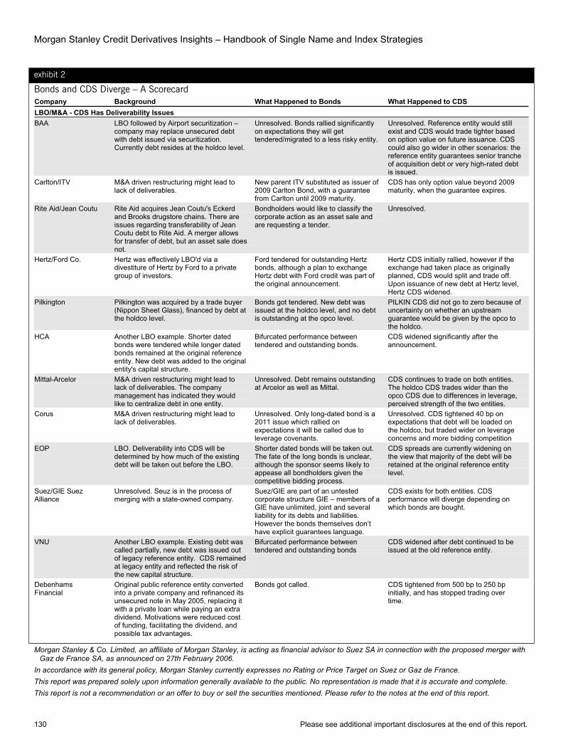
Morgan Stanley Credit Derivatives Insights – Handbook of Single Name and Index Strategies
130 Please see additional important disclosures at the end of this report.
exhibit 2
Bonds and CDS Diverge – A Scorecard Company Background What Happened to Bonds What Happened to CDS LBO/M&A - CDS Has Deliverability Issues BAA LBO followed by Airport securitization –
company may replace unsecured debt with debt issued via securitization. Currently debt resides at the holdco level.
Unresolved. Bonds rallied significantly on expectations they will get tendered/migrated to a less risky entity.
Unresolved. Reference entity would still exist and CDS would trade tighter based on option value on future issuance. CDS could also go wider in other scenarios: the reference entity guarantees senior tranche of acquisition debt or very high-rated debt is issued.
Carlton/ITV M&A driven restructuring might lead to lack of deliverables.
New parent ITV substituted as issuer of 2009 Carlton Bond, with a guarantee from Carlton until 2009 maturity.
CDS has only option value beyond 2009 maturity, when the guarantee expires.
Rite Aid/Jean Coutu Rite Aid acquires Jean Coutu's Eckerd and Brooks drugstore chains. There are issues regarding transferability of Jean Coutu debt to Rite Aid. A merger allows for transfer of debt, but an asset sale does not.
Bondholders would like to classify the corporate action as an asset sale and are requesting a tender.
Unresolved.
Hertz/Ford Co. Hertz was effectively LBO'd via a divestiture of Hertz by Ford to a private group of investors.
Ford tendered for outstanding Hertz bonds, although a plan to exchange Hertz debt with Ford credit was part of the original announcement.
Hertz CDS initially rallied, however if the exchange had taken place as originally planned, CDS would split and trade off. Upon issuance of new debt at Hertz level, Hertz CDS widened.
Pilkington Pilkington was acquired by a trade buyer (Nippon Sheet Glass), financed by debt at the holdco level.
Bonds got tendered. New debt was issued at the holdco level, and no debt is outstanding at the opco level.
PILKIN CDS did not go to zero because of uncertainty on whether an upstream guarantee would be given by the opco to the holdco.
HCA Another LBO example. Shorter dated bonds were tendered while longer dated bonds remained at the original reference entity. New debt was added to the original entity's capital structure.
Bifurcated performance between tendered and outstanding bonds.
CDS widened significantly after the announcement.
Mittal-Arcelor M&A driven restructuring might lead to lack of deliverables. The company management has indicated they would like to centralize debt in one entity.
Unresolved. Debt remains outstanding at Arcelor as well as Mittal.
CDS continues to trade on both entities. The holdco CDS trades wider than the opco CDS due to differences in leverage, perceived strength of the two entities.
Corus M&A driven restructuring might lead to lack of deliverables.
Unresolved. Only long-dated bond is a 2011 issue which rallied on expectations it will be called due to leverage covenants.
Unresolved. CDS tightened 40 bp on expectations that debt will be loaded on the holdco, but traded wider on leverage concerns and more bidding competition
EOP LBO. Deliverability into CDS will be determined by how much of the existing debt will be taken out before the LBO.
Shorter dated bonds will be taken out. The fate of the long bonds is unclear, although the sponsor seems likely to appease all bondholders given the competitive bidding process.
CDS spreads are currently widening on the view that majority of the debt will be retained at the original reference entity level.
Suez/GIE Suez Alliance
Unresolved. Seuz is in the process of merging with a state-owned company.
Suez/GIE are part of an untested corporate structure GIE – members of a GIE have unlimited, joint and several liability for its debts and liabilities. However the bonds themselves don’t have explicit guarantees language.
CDS exists for both entities. CDS performance will diverge depending on which bonds are bought.
VNU Another LBO example. Existing debt was called partially, new debt was issued out of legacy reference entity. CDS remained at legacy entity and reflected the risk of the new capital structure.
Bifurcated performance between tendered and outstanding bonds
CDS widened after debt continued to be issued at the old reference entity.
Debenhams Financial
Original public reference entity converted into a private company and refinanced its unsecured note in May 2005, replacing it with a private loan while paying an extra dividend. Motivations were reduced cost of funding, facilitating the dividend, and possible tax advantages.
Bonds got called. CDS tightened from 500 bp to 250 bp initially, and has stopped trading over time.
Morgan Stanley & Co. Limited, an affiliate of Morgan Stanley, is acting as financial advisor to Suez SA in connection with the proposed merger with Gaz de France SA, as announced on 27th February 2006.
In accordance with its general policy, Morgan Stanley currently expresses no Rating or Price Target on Suez or Gaz de France. This report was prepared solely upon information generally available to the public. No representation is made that it is accurate and complete. This report is not a recommendation or an offer to buy or sell the securities mentioned. Please refer to the notes at the end of this report.

Section B, Chapter 26 “Worthless” Protection?
Please see additional important disclosures at the end of this report. 131
exhibit 2
Bonds and CDS Diverge – A Scorecard (cont'd) Company Background What Happened to Bonds What Happened to CDS Spin-off/Divestiture Alltel A stereotypical example of recent telecom
spin-offs – Alltel monetized assets on balance sheet (wireline business) that has a relatively low tax base and underleveraged. The company swapped existing debt for new debt issued by the new wireline entity. The swap was executed "in conjunction with" the event, triggering succession language.
Very short end bonds benefited from tenders, longer term bonds benefited from decreased leverage at the original entity level.
CDS split between Alltel and the new wireline business Windstream. The new entity was more highly levered and the weighted average impact was a widening in CDS spreads right after the spin-off.
Cendant/Avis Legacy reference entity Cendant split into various segments. Debt at legacy entity was paid down in full in a manner that would not trigger succession language.
Fully paid, bonds benefited from tenders.
Spreads tightened initially, however reversed direction on the view that old Cendant reference entity is essentially a holdco for Avis and new debt (especially in relation to a future LBO) might be issued out of it.
FKI A sale of businesses by FKI may force the company to buy back its bonds ahead of corporate action (to avoid a technical default).
Plans not announced yet. CDS should go to 0/option value based on the bonds being called. However, company announced it will consider "looking after credit default swap holders". They could reissue additional debt at the same entity.
GUS Demerger of credit business from retail business could lead to CDS becoming worthless.
Uncertainty on whether the bonds will be tendered for/terms of the tender. Company agreed to change the terms of the bonds and left bonds outstanding.
CDS was quite volatile within a range of 35-55 bp due to the uncertainty about both existing bonds and new issuance. A new holdco was created which led to worries about lack of new bonds at the opco.
Sprint Sprint’s spin-off of Embarq. In this case, succession language was not triggered as total amount of debt transferred did not exceed the 25% threshold.
Inter-company debt exchange. Sprint CDS widened before completion of spin-off and there was no significant move in spreads after completion.
Tyco Announced a plan to separate the company's current portfolio of diverse businesses into three publicly traded companies.
Existing debt is expected to be allocated among the three companies or refinanced. The bonds rallied in anticipation of a tender.
CDS trading tight, but started trading up slightly since mid-December. It is not clear whether succession language will be triggered.
Verizon Verizon spun off of Yellow Pages business to Idearc and reduced total debt by more than 7 billion in a debt-for-debt exchange.
A portion of the debt got tendered. CDS split between Verizon and Idearc. Idearc CDS initially widened, but tightened later on once Idearc bonds priced
Six Continents Plc De-merger into pubs and hotels. Initially proposed structure stated the company's intention to tender for all bonds prior to de-merger, then issue new debt at Intercontinental Hotels entity. Rationalization of business into hotels and pubs entities.
Six Continents Successor. A small piece of debt was left outstanding.
Ultimately guarantees from Int Hotels and a piece of Six Continents debt outstanding left CDS with deliverables. CDS rallied initially on the fear of lack of deliverables. Subsequently widened but not to earlier levels.
Morgan Stanley Credit Derivatives Insights – Handbook of Single Name and Index Strategies
132 Please see additional important disclosures at the end of this report.
exhibit 2
Bonds and CDS Diverge – A Scorecard (cont'd) Company Background What Happened to Bonds What Happened to CDS Pure Refinancing Colt UK Plc Colt Telecom raised equity to pay-off
existing debt and deleverage. Bonds get bought out, except for the ‘09s.
CDS gapped in tighter around 200 bp tighter. CDS could potentially gap in further in future if new debt is issued only out of the holdco and the ‘09s mature.
Liberty Global/Cablecom
New bond issuance came out of the opco (Cablecom), when the market expected the bonds to be issued at the holdco level.
- CDS gapped more than 200 bp wider on the unexpected issuance.
Rentokil Initial Plc Company does not have enough distributable reserves to continue paying dividends, so they executed a sale to a new holding company, to create the surplus and payout a dividend. A new holdco CDS started trading while the opco CDS stopped trading.
No opco bonds were left outstanding. Holdco CDS started trading while opco CDS became worthless, trading to option value on new issuance.
BCP Caylux Holdings (Celanese)
Restructuring moving company's debt and assets to BCP Crystal US Holdings, making it successor entity. New contracts may have been written on original entity subsequent to the transfer, hence not automatically governed by successor language.
Bonds transferred to BCP Crystal US Holdings.
BCP Crystal US Holdings Successor.
Land Securities Plc Land Securities Plc changed its funding structure by issuing ‘hybrid’ secured debt. Existing bondholders, both secured and unsecured, were offered to switch their exposure to the new secured structure.
Achieving higher leverage while maintaining a degree of flexibility for management to operate and trade property as part of business.
Bonds exchanged for new secured notes. CDS quoted tighter from 35 to 10 bp. No successor, given the nature of the bond exchange. CDS on the original reference entity remained outstanding with no deliverables.
Source: Morgan Stanley

Please see additional important disclosures at the end of this report. 133
Chapter 27
Recovery Lessons
Primary Analyst: Sivan Mahadevan Primary Analyst: Peter Polanskyj Primary Analyst: Pinar Onur
Two of the most interesting developments last year in the single-name space were the ISDA-coordinated global protocol to settle credit events and the emergence of recovery locks as a means to hedge recovery risk. The two themes, in fact, are quite inter-related, as recovery locks are a play on recovery during the period immediately following bankruptcy filing, which is in many cases determined by the auction process under the global protocol. The market now has experience with global settlements on five bankrupt US companies (see Exhibit 1) and recovery locks were actively traded on two.
exhibit 1
Auctions Administered Under the ISDA Global CDS Protocol
Credit Bankruptcy Filing Date
CDSAuction
Date
No. ofAdhering
PartiesFinalPrice
Quebecor World 01/21/2008 02/19/2008 589 41.25Movie Gallery (LCDS) 10/16/2007 10/23/2007 NA 91.5Dura Senior 10/30/2006 11/28/2006 NA 24.125Dura Sub 10/30/2006 11/28/2006 NA 3.5Dana 3/3/2006 3/31/2006 340 75Calpine 12/20/2005 1/17/2006 323 19.125Delphi 10/10/2005 11/4/2005 577 63.375Delta 9/15/2005 10/11/2005 71 18Northwest 9/15/2005 10/11/2005 71 28Collins & Aikman (Senior) 5/17/2005 6/14/2005 454 43.625Collins & Aikman (Sub) 5/17/2005 6/23/2005 NA 6.375
Source: Morgan Stanley, ISDA, CreditEx, Markit
Since we published our first thoughts on recovery locks a few months ago, we have witnessed a greater than expected acceptance of the instruments among investors, partly as a result of recent credit events.1 In the month leading up to the bankruptcy filing, unsecured Calpine recovery locks traded very close (17% to 20% range) to Calpine’s ultimate recovery in the global settlement (19.125%). Delphi was less stable, with recovery locks at lower levels compared to the recovery value that came out of the auction. The only issue we have seen was inconsistency among dealers with notice of physical settlement (NOPS) language. In a recovery lock, the seller of protection may have an economic incentive to trigger a contract (i.e., when the actual recovery is higher than “locked” in, the recovery lock buyer will want to trigger), so it is important that recovery locks allows for NOPS from either party, in our view.
1Please refer to Chapter 5.
We remind investors that recovery locks are not instruments for recovery risk management through the whole bankruptcy process, instead they are meant for short-term recovery management (post-bankruptcy until CDS settlement). As such, they are actually good instruments to use in strategies with existing CDS, CDX, or index tranche positions, given the increased fungibility with these instruments. We go through our thoughts on how recovery locks can be incorporated into to the credit portfolio management process in this chapter and see if we can learn anything from the auction process.
WHAT CAN WE OPINE FROM THE GLOBAL CDS PROTOCOL? In Exhibit 2 we show the market price of selected deliverable obligations for the CKC, DPH and CPN settlement auctions, focused on the period immediately surrounding the actual credit events. For both Delphi and Calpine, deliverable bonds rallied immediately following the credit events and prices remained generally higher through the auction. For Collins & Aikman, we did not see a similar rally, as pricing remained reasonably flat through the action settlement. But we would argue that the Collins & Aikman default was less well telegraphed given the significant price drop leading into the default.
exhibit 2
Price Shifts – Pre-Bankruptcy to Post-CDS Auction
Price
0
10
20
30
40
50
60
70
80
90
100
-60
-48
-36
-24
-12 0 12 24 36 48 60
Days From Bankruptcy Filing
CKC
DPH
CPN
Source: Morgan Stanley
While the bond price history in Exhibit 2 could indicate the CDS settlement process affected the trading of the underlying obligations, we find that, in these 3 cases at least, the impact was limited to about 10 points on the bonds. We caution that there is only a limited amount of data on this dynamic and therefore we consider any interpretation to be anecdotal. We are also reluctant to predict similar instances universally in the future (see below).
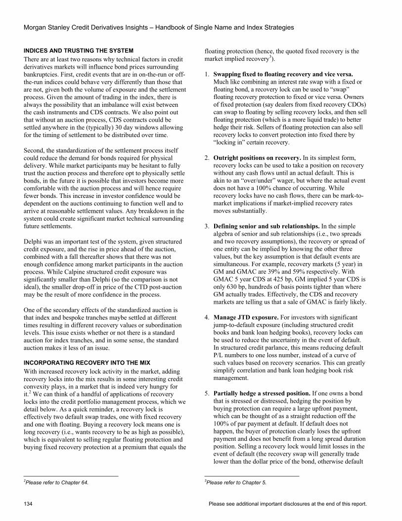
Morgan Stanley Credit Derivatives Insights – Handbook of Single Name and Index Strategies
134 Please see additional important disclosures at the end of this report.
INDICES AND TRUSTING THE SYSTEM There are at least two reasons why technical factors in credit derivatives markets will influence bond prices surrounding bankruptcies. First, credit events that are in on-the-run or off-the-run indices could behave very differently than those that are not, given both the volume of exposure and the settlement process. Given the amount of trading in the index, there is always the possibility that an imbalance will exist between the cash instruments and CDS contracts. We also point out that without an auction process, CDS contracts could be settled anywhere in the (typically) 30 day windows allowing for the timing of settlement to be distributed over time.
Second, the standardization of the settlement process itself could reduce the demand for bonds required for physical delivery. While market participants may be hesitant to fully trust the auction process and therefore opt to physically settle bonds, in the future it is possible that investors become more comfortable with the auction process and will hence require fewer bonds. This increase in investor confidence would be dependent on the auctions continuing to function well and to arrive at reasonable settlement values. Any breakdown in the system could create significant market technical surrounding future settlements.
Delphi was an important test of the system, given structured credit exposure, and the rise in price ahead of the auction, combined with a fall thereafter shows that there was not enough confidence among market participants in the auction process. While Calpine structured credit exposure was significantly smaller than Delphi (so the comparison is not ideal), the smaller drop-off in price of the CTD post-auction may be the result of more confidence in the process.
One of the secondary effects of the standardized auction is that index and bespoke tranches maybe settled at different times resulting in different recovery values or subordination levels. This issue exists whether or not there is a standard auction for index tranches, and in some sense, the standard auction makes it less of an issue.
INCORPORATING RECOVERY INTO THE MIX With increased recovery lock activity in the market, adding recovery locks into the mix results in some interesting credit convexity plays, in a market that is indeed very hungry for it.2 We can think of a handful of applications of recovery locks into the credit portfolio management process, which we detail below. As a quick reminder, a recovery lock is effectively two default swap trades, one with fixed recovery and one with floating. Buying a recovery lock means one is long recovery (i.e., wants recovery to be as high as possible), which is equivalent to selling regular floating protection and buying fixed recovery protection at a premium that equals the
2Please refer to Chapter 64.
floating protection (hence, the quoted fixed recovery is the market implied recovery3).
1. Swapping fixed to floating recovery and vice versa. Much like combining an interest rate swap with a fixed or floating bond, a recovery lock can be used to “swap” floating recovery protection to fixed or vice versa. Owners of fixed protection (say dealers from fixed recovery CDOs) can swap to floating by selling recovery locks, and then sell floating protection (which is a more liquid trade) to better hedge their risk. Sellers of floating protection can also sell recovery locks to convert protection into fixed there by “locking in” certain recovery.
2. Outright positions on recovery. In its simplest form, recovery locks can be used to take a position on recovery without any cash flows until an actual default. This is akin to an “over/under” wager, but where the actual event does not have a 100% chance of occurring. While recovery locks have no cash flows, there can be mark-to-market implications if market-implied recovery rates moves substantially.
3. Defining senior and sub relationships. In the simple algebra of senior and sub relationships (i.e., two spreads and two recovery assumptions), the recovery or spread of one entity can be implied by knowing the other three values, but the key assumption is that default events are simultaneous. For example, recovery markets (5 year) in GM and GMAC are 39% and 59% respectively. With GMAC 5 year CDS at 425 bp, GM implied 5 year CDS is only 630 bp, hundreds of basis points tighter than where GM actually trades. Effectively, the CDS and recovery markets are telling us that a sale of GMAC is fairly likely.
4. Manage JTD exposure. For investors with significant jump-to-default exposure (including structured credit books and bank loan hedging books), recovery locks can be used to reduce the uncertainty in the event of default. In structured credit parlance, this means reducing default P/L numbers to one loss number, instead of a curve of such values based on recovery scenarios. This can greatly simplify correlation and bank loan hedging book risk management.
5. Partially hedge a stressed position. If one owns a bond that is stressed or distressed, hedging the position by buying protection can require a large upfront payment, which can be thought of as a straight reduction off the 100% of par payment at default. If default does not happen, the buyer of protection clearly loses the upfront payment and does not benefit from a long spread duration position. Selling a recovery lock would limit losses in the event of default (the recovery swap will generally trade lower than the dollar price of the bond, otherwise default
3Please refer to Chapter 5.
Section B, Chapter 27 Recovery Lessons
Please see additional important disclosures at the end of this report. 135
is 100% certain), but no cash flows are required, and the investor still keeps most of the spread duration in case the credit rallies. There are MTM risks on the recovery lock, but this could be less severe than CDS movements.
6. Debt/equity strategies. The credit leg of debt/equity strategies generally involves using CDS even though the investor may want the “default option” component of the CDS more than the spread duration component. In fact, the failure of many debt/equity strategies can be blamed on long protection positions in the face of significant credit rallies. A recovery lock can be used instead, where the payout would only be at default and only if one is right about a recovery view. Again, we caution about MTM issues on the recovery lock, but they could be more muted than straight CDS.
7. Hedging general company risk. It has become increasingly common for corporations to hedge exposure they have to other companies (through receivables and the like) by using default swaps. Selling a recovery lock could be another way of hedging this risk, the idea being that a lower recovery default would negatively impact any claim by a corporate with receivables exposure, so the recovery lock would help to hedge this risk. The recovery lock (with no cash flows) may be a cheaper hedge to owning protection.
8. Credit I/O risk from unwinds. There is a lot of credit I/O risk in the markets given all of the CDS unwind activity.4 In an unwind where premiums have moved a lot from where trades were put on, investors often ask to unwind earlier positions rather than keeping two legs alive. This eliminates the I/O risk (for the investor) when a credit event occurs. Dealers calculate the unwind value in part by making a recovery assumption, and this recovery assumption can be hedged (to some degree) with a recovery lock.
CONCLUSION – THE MARKETS FORCE MATURITY Enough has happened over the past few months for us to state that recovery markets are a bit more mature. We find numerous applications of recovery instruments in the credit portfolio management process, given different duration and default exposure of the instruments relative to plain vanilla CDS. However, we remind investors that market activity in recovery instruments is limited to only a handful of credits, so building out portfolio strategies is difficult.
4Please refer to Chapter 23.
Morgan Stanley Credit Derivatives Insights – Handbook of Single Name and Index Strategies
136 Please see additional important disclosures at the end of this report.
Chapter 28
The Recovery Market’s Next Leg – Indices October 20, 2006
Primary Analyst: Sivan Mahadevan Primary Analyst: Phanikiran Naraparaju Primary Analyst: Pinar Onur Primary Analyst: Andrew Sheets
As the market for “recovery” instruments continues to gain momentum, a new dimension is coming to the surface: fixed recovery swaps on indices. These relatively new instruments complement single-name recovery products (recovery swaps) and synthetic CDOs with fixed recovery swaps on the underlying names. In our view, each of these three areas is quite distinct, with different valuation approaches and technical factors.1
The single-name recovery market has garnered significant attention over the past 18 months, and there have been a handful of good tests for this market among defaulted US credits (Delphi, Calpine and Dana). We remind investors that trading recovery risk is nothing new to the credit derivatives markets (early instruments were fixed recovery in nature), but with the advent of standardization and the goal of making the CDS contract as bond-like as possible, separate recovery information was lost in the process, in favor of “floating” recovery or physical settlement in standard CDS contracts.
On the portfolio side, fixed recovery CDOs have existed for years, and even gained some momentum as we move beyond the 2002 corporate environment, when low recoveries were feared. Ratings agencies give some benefit for the certainty that comes along with fixed recovery on the underlying names in CDOs, but high recovery defaults recently have led to some underperformance in these early deals (where recovery was generally fixed in the 35% to 40% range). Today we are also seeing deals with significantly higher fixed recoveries.
Although it is still early in the market, we believe that fixed recovery on straight untranched portfolios (or indices) will behave somewhat differently from the other two parts of the recovery market (single-names and CDOs). For the purposes of this chapter, we focus on zero-recovery swaps on the popular European indices (iTraxx Main, HiVol and XOver).
We will go through the details of our view on fixed recovery indices in this chapter, but here are the main points.
• We are beginning to see activity in zero recovery swaps on the iTraxx indices. Rather than focusing on implied recovery values, it is perhaps simplest to think of zero recovery iTraxx instruments as subordinated debt or a more levered play on default risk.
1For earlier thoughts on recovery swaps, please see chapters 5 and 27 and “Recovery Trading: Unbundling the Credit Risk Package,” November 18, 2005.
• Long investors get increased yield for pure default exposure, while short investors lean against implied recoveries for a more explicit bet on default risk. Market beta and DV01 measures are important to consider in this context.
• Removing recovery uncertainly adds value, a fact that agencies acknowledge in their CDO ratings. By isolating default risk, investors can bet on embedded IG risk premiums, something markets have historically overestimated.
• Current market pricing implies a low index recovery (high 30s). This is in direct contrast to the strongest recovery environment on record (averaging mid-50s), which we are in right now.
• Index recovery products are also influenced by structured credit technicals, in this case related to fixed recovery CDOs. Fixed Recovery CDO Flows can push implied recovery lower, especially on the IG indices.
• For lots of reasons, there is tendency for implied recovery on specific companies to be high today, but this is not an argument for implied recovery to be high on an index of credits that is far away from default.
• One of the big differences between indices and a single credit is that the single-name has much more jump-to-default risk (for a given notional size, given the lack of diversity). The JTD risk premium pushes implied recovery values in the market higher, in today’s high recovery environment. The opposite would probably be true in a more negative credit environment.
• In the current environment, recovery on low-quality names could be a bit higher because the names are more likely to go through a recovery process that is well supported. The argument for recoveries falling when defaults rise is well understood historically; the opposite seems to be true in the pricing of index recovery instruments.
ITRAXX ZERO RECOVERY INDICES While we refer to this space broadly as the recovery market, from an index perspective, most of the activity we see is in the form of zero recovery CDS rather than the recovery swap (which can be easily derived from the former, see Appendix A). Like its name implies, a zero recovery CDS contract is effectively identical to a standard CDS contract on the index, except that any credit event would be settled with a 0% recovery (buyer of protection would receive 100% of the notional and neither pay nor deliver anything to the seller of protection).

Section B, Chapter 28 The Recovery Market’s Next Leg – Indices
Please see additional important disclosures at the end of this report. 137
A zero recovery CDS (ZRCDS) on the iTraxx indices can be viewed like generic subordinated debt. The higher spread that one earns by selling protection is compensation for zero recovery at default, so assuming both contracts are triggered by the same credit events, one can compute implied recoveries from both legs of the trade. But implied recovery is not the only difference. A zero recovery CDS contract is also more levered (i.e., a higher beta product) relative to standard floating recovery protection. So measures like beta and duration will differ, as well.
exhibit 1
Zero Recovery iTraxx Indices (5-Year Maturity) Main6 HiVol6 Xover6Index 27.4 51.5 259.5ZRCDS spread (mid) 41.5 81.25 405.25Recovery (Mid) 34.0% 36.5% 36.0%Annualized Def. Probability 0.42% 0.81% 4.05%Historical Def. Probability 0.26% 0.47% 5.93%Spread Beta 1.52 1.57 1.56Index Sprd DV01 (bp) 4.71 4.66 4.27ZRCDS Sprd DV01 (bp) 7.13 7.28 6.78ZRCDS DV R01 (bp) 3.08 6.14 29.03ZR Index Default Impact -0.8% -3.3% -2.2%Breakeven Defaults 2.5 1.1 8.5Breakeven Default Rate 2.0% 3.7% 18.9%
ZRCDS DV01: Change in Dollar Value of the ZRCDS for 1 bp change in the standard CDS.
ZRCDS DV R01: Change in Dollar Value of the ZRCDS for 1% change in the Recovery Swap (but same index spread). Spread Beta: ZRCDS spread change for 1 bp change in CDS spread, unchanged recovery. Breakeven Defaults and Default Rate: Given investor is long ZRCDS. Assume defaults evenly spaced, and assumes no discounting factor.
Source: Morgan Stanley
In Exhibit 1, we show levels for iTraxx indices (Main, HiVol and XOver) for both standard (floating) recovery and 0% recovery. From these levels, fairly simple algebra will give us implied recovery, and CDSW pricing engines can give us DV01 type measures.
• The ZRCDS spread is the same as annualized default probability of the credit, i.e., current XOver and IG default rates are 4.05% and 0.42%, respectively.
• The spread duration (to standard CDS spread) of the ZRCDS is roughly 1.5-1.6X that of standard CDS, currently about 6.78 for the main ZRCDS. The spread DV01 keeps increasing as the implied recovery rises.
• The ZRCDS is also sensitive to recovery moves: a one-point change in recovery translates to 3.08 bp in the mark-to-market of the IG ZRCDS. The higher the default probability, the greater the DVR01; for example, the XOver index has a DVR01 of 29.03 bp, roughly 10 times that of the IG index.
• It takes about eight defaults to break even on the XOver ZRCDS (assuming no discounting factor). The break-even number of defaults for the main and HiVol ZRCDS index are 2.5 and 1.1, respectively.
MARKET ACTIVITY – ZERO RECOVERY INDICES To be clear, market activity in zero recovery iTraxx indices has been limited and has been in existence by our measures only since the spring of this year. Investor participation appears to be mainly from hedge funds/proprietary desks and structured credit hedgers, and even dealer activity is limited. But given broader interest level in zero recovery CDS on single-names, we expect activity to pick up at the index level, as well, perhaps once a bit more standardization appears in the index market.
A primary motivation for many investors, very simply put, appears to be yield. Investors who have sold outright protection on zero recovery indices or single names have been comfortable enough with default risk (either at the single-name or market level) to lever the view with 0% recovery. Additionally appealing, from both the long and the short side, is that ZRCDS makes credit an explicit bet on defaults, rather than default and recovery.
The subordinated nature of ZRCDS makes it behave as a high beta instrument – which can create interesting opportunities from a breakeven default perspective. When XOver traded off earlier in the year from around 230 bp to 290 bp, implied recovery moved higher by about 5% to 39%. The ZRCDS thus widened 127 bp to 475 bp, with recovery repricing accounting for 36 bp of the spread widening. The break-even number of defaults would be as many as 10 defaults (assuming periodic defaults and no discounting factors). The incremental beta added because of recovery repricing could reduce at wider spread levels as investors become attracted to locking in high recoveries by selling ZRCDS protection and buying excess (beta weighted) CDS protection.
TODAY’S RECOVERY MARKET: A BIT NON-INTUITIVE Before we attempt to explain pricing in zero recovery indices (which requires a view on implied recovery at the index level), we feel it is important to discuss the current recovery market to some degree. We live in a high recovery world today (see Exhibit 2) for lots of reasons, including the fact that the US and Europe are not in recessions or high default environments, the healthy bid in the market for distressed assets, and enormous derivative volumes, which can lead to some imbalances when default events have to be settled. For these reasons, single-name recovery swaps tend to trade at levels (40% to 70%) that are higher than historical average recoveries.
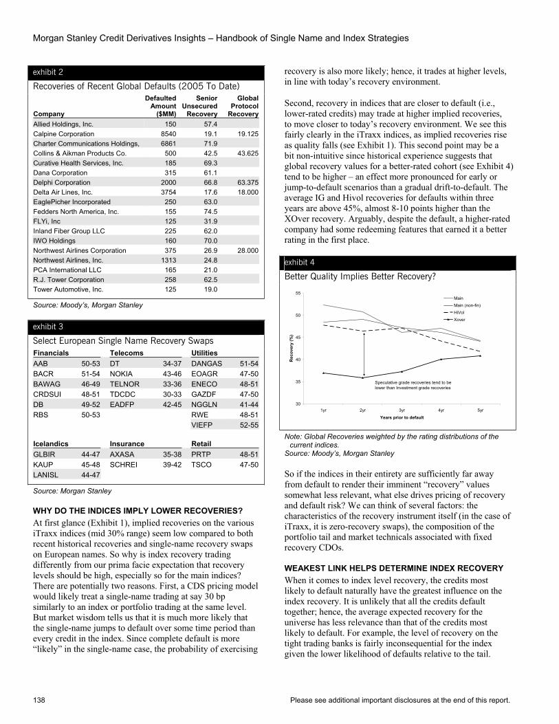
Morgan Stanley Credit Derivatives Insights – Handbook of Single Name and Index Strategies
138 Please see additional important disclosures at the end of this report.
exhibit 2
Recoveries of Recent Global Defaults (2005 To Date)
Company
Defaulted Amount
($MM)
Senior Unsecured
Recovery
Global Protocol
RecoveryAllied Holdings, Inc. 150 57.4 Calpine Corporation 8540 19.1 19.125Charter Communications Holdings, 6861 71.9 Collins & Aikman Products Co. 500 42.5 43.625Curative Health Services, Inc. 185 69.3 Dana Corporation 315 61.1 Delphi Corporation 2000 66.8 63.375Delta Air Lines, Inc. 3754 17.6 18.000EaglePicher Incorporated 250 63.0 Fedders North America, Inc. 155 74.5 FLYi, Inc 125 31.9 Inland Fiber Group LLC 225 62.0 IWO Holdings 160 70.0 Northwest Airlines Corporation 375 26.9 28.000Northwest Airlines, Inc. 1313 24.8 PCA International LLC 165 21.0 R.J. Tower Corporation 258 62.5 Tower Automotive, Inc. 125 19.0
Source: Moody’s, Morgan Stanley
exhibit 3
Select European Single Name Recovery Swaps Financials Telecoms Utilities AAB 50-53 DT 34-37 DANGAS 51-54BACR 51-54 NOKIA 43-46 EOAGR 47-50BAWAG 46-49 TELNOR 33-36 ENECO 48-51CRDSUI 48-51 TDCDC 30-33 GAZDF 47-50DB 49-52 EADFP 42-45 NGGLN 41-44RBS 50-53 RWE 48-51 VIEFP 52-55 Icelandics Insurance Retail GLBIR 44-47 AXASA 35-38 PRTP 48-51KAUP 45-48 SCHREI 39-42 TSCO 47-50LANISL 44-47
Source: Morgan Stanley
WHY DO THE INDICES IMPLY LOWER RECOVERIES? At first glance (Exhibit 1), implied recoveries on the various iTraxx indices (mid 30% range) seem low compared to both recent historical recoveries and single-name recovery swaps on European names. So why is index recovery trading differently from our prima facie expectation that recovery levels should be high, especially so for the main indices? There are potentially two reasons. First, a CDS pricing model would likely treat a single-name trading at say 30 bp similarly to an index or portfolio trading at the same level. But market wisdom tells us that it is much more likely that the single-name jumps to default over some time period than every credit in the index. Since complete default is more “likely” in the single-name case, the probability of exercising
recovery is also more likely; hence, it trades at higher levels, in line with today’s recovery environment.
Second, recovery in indices that are closer to default (i.e., lower-rated credits) may trade at higher implied recoveries, to move closer to today’s recovery environment. We see this fairly clearly in the iTraxx indices, as implied recoveries rise as quality falls (see Exhibit 1). This second point may be a bit non-intuitive since historical experience suggests that global recovery values for a better-rated cohort (see Exhibit 4) tend to be higher – an effect more pronounced for early or jump-to-default scenarios than a gradual drift-to-default. The average IG and Hivol recoveries for defaults within three years are above 45%, almost 8-10 points higher than the XOver recovery. Arguably, despite the default, a higher-rated company had some redeeming features that earned it a better rating in the first place.
exhibit 4
Better Quality Implies Better Recovery?
30
35
40
45
50
55
1yr 2yr 3yr 4yr 5yr
Years prior to default
Rec
over
y (%
)MainMain (non-fin)HiVolXover
Speculative grade recoveries tend to be lower than Investment grade recoveries
Note: Global Recoveries weighted by the rating distributions of the current indices.
Source: Moody’s, Morgan Stanley
So if the indices in their entirety are sufficiently far away from default to render their imminent “recovery” values somewhat less relevant, what else drives pricing of recovery and default risk? We can think of several factors: the characteristics of the recovery instrument itself (in the case of iTraxx, it is zero-recovery swaps), the composition of the portfolio tail and market technicals associated with fixed recovery CDOs.
WEAKEST LINK HELPS DETERMINE INDEX RECOVERY When it comes to index level recovery, the credits most likely to default naturally have the greatest influence on the index recovery. It is unlikely that all the credits default together; hence, the average expected recovery for the universe has less relevance than that of the credits most likely to default. For example, the level of recovery on the tight trading banks is fairly inconsequential for the index given the lower likelihood of defaults relative to the tail.
Section B, Chapter 28 The Recovery Market’s Next Leg – Indices
Please see additional important disclosures at the end of this report. 139
As of now, the non-HiVol part of the tail is dominated by consumer credits followed by TMT, the same sectors which resulted in low recoveries in the 2001-2003 credit cycle. This partly explains the low recovery on the indices despite the high single name recoveries in various sectors.
RISK PREMIUM AND FIXED RECOVERY CDO FLOWS As we have noted previously in our research, risk and liquidity premiums (over and above default compensation) are generally higher in IG spreads than in the HY space – hence the huge IG structured issuance. This IG risk premium could manifest itself in both the default probability (higher than expected) and implied recovery (lower than expected).
An important technical for the fixed recovery index market in this context is flows from fixed recovery CDOs. The reduced uncertainty associated with fixed recoveries provides a bit of a ratings boost to bespoke tranches, and there is a reasonable flow into fixed recovery CDOs for this reason. Further, the simplicity of knowing exactly how many defaults it takes to touch a tranche is a popular driver of flows, as well.
Fixed recovery CDO activity by itself has a bias to push the implied recoveries lower. Structured credit desks can effectively sell fixed recovery protection into the market and buy floating recovery protection, which is equivalent to being
a net seller of recovery in a recovery swap sense. What this means is that the risk premiums on the default probability side find an outlet via fixed recovery CDOs, but there is no similar equivalent on the recovery side leading to suppressed implied recoveries. This could be another explanation for why higher quality iTraxx Main recovery trades at lower levels than the lower quality HiVol and XOver indices (given the preference for higher quality credit in bespokes).
CONCLUSIONS – THINK SUBORDINATED DEBT There are some good technical reasons why the implied recovery on the indices trades at levels that are lower than lower quality single-names, however non-intuitive it may feel. And as investors continue to be comfortable with the current low default environment, we could find zero recovery protection on the iTraxx indices trading at these levels or even tighter relative to standard floating recovery indices (pushing implied recovery even lower).
From an investment strategy perspective, we believe it makes more sense to think of zero recovery index protection as subordinate debt, or a more levered way to gain exposure to the same set of credits. With this leverage comes market beta and different sensitivities to spread moves, which investors need to be aware of.
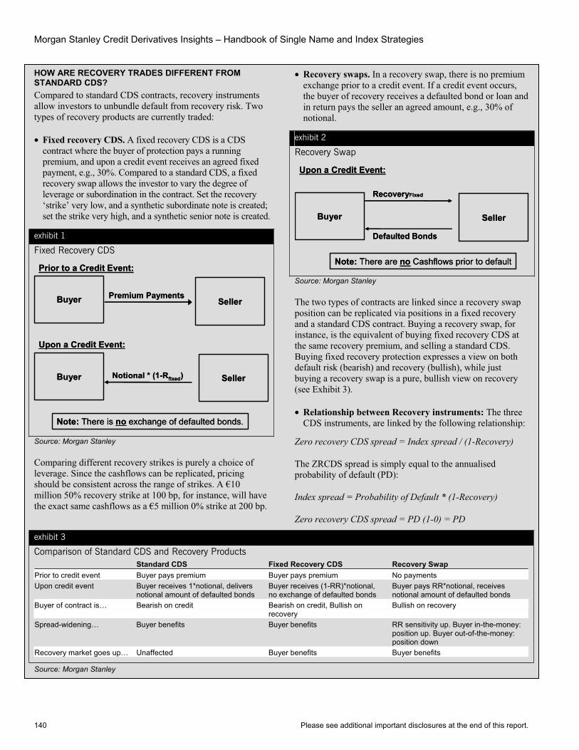
Morgan Stanley Credit Derivatives Insights – Handbook of Single Name and Index Strategies
140 Please see additional important disclosures at the end of this report.
HOW ARE RECOVERY TRADES DIFFERENT FROM STANDARD CDS? Compared to standard CDS contracts, recovery instruments allow investors to unbundle default from recovery risk. Two types of recovery products are currently traded:
• Fixed recovery CDS. A fixed recovery CDS is a CDS contract where the buyer of protection pays a running premium, and upon a credit event receives an agreed fixed payment, e.g., 30%. Compared to a standard CDS, a fixed recovery swap allows the investor to vary the degree of leverage or subordination in the contract. Set the recovery ‘strike’ very low, and a synthetic subordinate note is created; set the strike very high, and a synthetic senior note is created.
exhibit 1
Fixed Recovery CDS
Buyer Seller
Prior to a Credit Event:
Premium Payments
Buyer Seller
Upon a Credit Event:
Notional * (1-Rfixed)
Note: There is no exchange of defaulted bonds.
Buyer Seller
Prior to a Credit Event:
Premium Payments
Buyer Seller
Upon a Credit Event:
Notional * (1-Rfixed)
Note: There is no exchange of defaulted bonds.
Source: Morgan Stanley
Comparing different recovery strikes is purely a choice of leverage. Since the cashflows can be replicated, pricing should be consistent across the range of strikes. A €10 million 50% recovery strike at 100 bp, for instance, will have the exact same cashflows as a €5 million 0% strike at 200 bp.
• Recovery swaps. In a recovery swap, there is no premium exchange prior to a credit event. If a credit event occurs, the buyer of recovery receives a defaulted bond or loan and in return pays the seller an agreed amount, e.g., 30% of notional.
exhibit 2
Recovery Swap
Buyer Seller
Upon a Credit Event:
Defaulted Bonds
Note: There are no Cashflows prior to default
RecoveryFixed
Buyer Seller
Upon a Credit Event:
Defaulted Bonds
Note: There are no Cashflows prior to default
RecoveryFixed
Source: Morgan Stanley
The two types of contracts are linked since a recovery swap position can be replicated via positions in a fixed recovery and a standard CDS contract. Buying a recovery swap, for instance, is the equivalent of buying fixed recovery CDS at the same recovery premium, and selling a standard CDS. Buying fixed recovery protection expresses a view on both default risk (bearish) and recovery (bullish), while just buying a recovery swap is a pure, bullish view on recovery (see Exhibit 3).
• Relationship between Recovery instruments: The three CDS instruments, are linked by the following relationship:
Zero recovery CDS spread = Index spread / (1-Recovery)
The ZRCDS spread is simply equal to the annualised probability of default (PD):
Index spread = Probability of Default * (1-Recovery)
Zero recovery CDS spread = PD (1-0) = PD
exhibit 3
Comparison of Standard CDS and Recovery Products Standard CDS Fixed Recovery CDS Recovery Swap Prior to credit event Buyer pays premium Buyer pays premium No payments Upon credit event Buyer receives 1*notional, delivers
notional amount of defaulted bonds Buyer receives (1-RR)*notional, no exchange of defaulted bonds
Buyer pays RR*notional, receives notional amount of defaulted bonds
Buyer of contract is… Bearish on credit Bearish on credit, Bullish on recovery
Bullish on recovery
Spread-widening… Buyer benefits Buyer benefits RR sensitivity up. Buyer in-the-money: position up. Buyer out-of-the-money: position down
Recovery market goes up… Unaffected Buyer benefits Buyer benefits
Source: Morgan Stanley
Please see additional important disclosures at the end of this report. 141
Chapter 29
What Exactly Is Index Arb? September 15, 2006
Primary Analyst: Sivan Mahadevan Primary Analyst: Peter Polanskyj Primary Analyst: Pinar Onur Primary Analyst: Andrew Sheets Primary Analyst: Phanikiran Naraparaju
The notion that CDS indices have boosted credit market trading volumes, introduced market transparency and have brought in a whole new set of credit investors and speculators is at this point a truism. What may not be so obvious is that index arbitrage activity, which is practiced only by a few market participants, is also changing the character of the credit markets, forcing an “instant” synchronization of macro credit activity on underlying bonds and CDS. For these reasons, any activity in the indices cannot be ignored, even by those who dread the behavior of short-term oriented investors.
What causes the dislocations between indices and underlying names in the first place? The answer, very simply put, is flows, sometimes massive flows. Bid lists for protection (BWICs) related to structured credit activity often have lots of overlap with index constituents but may not actually involve the indices. At the other end, macro hedge funds can implement short-term views in size in the indices without ever executing a single-name trade. These are just two examples.
Based on our experiences, most active credit investors have heard of index arbitrage flows, or the act of “synchronizing” the price of indices with their underlying instruments and capturing any “mispricings.” On the surface, this is no different than it is in other markets where index products are also very active. But CDS index arbitrage is no simple exercise, neither from a basis risk nor operational perspective. Only those who can do both well can play, which is why it remains an art that only a few can practice.
To use an old Wall Street term, index arbitrage is a “ticket intensive” business in a derivatives market where everything trades OTC and not much is electronic yet. Executing can be a Herculean operational feat requiring several hundred transactions, which is the main reason why only a handful of players are prepared to participate. But it is also a business that requires taking other types of basis risks that can be very detailed in nature, but are indeed significant enough to make the entire strategy far from being a free lunch, even for those who are comfortable with the operational side of it. The remainder of this chapter is our attempt to give credit investors an appreciation for these risks, as we have been asked about it numerous times. In a nutshell, here is a laundry list of index arbitrage risk factors that we can think of.
• Liquidity: Indices can be significantly more liquid than the underlying names, particularly in high yield, where
single names may not trade much despite being part of actively traded indices.
• Maturity: Based on industry standard practices, 50% of the time, standard index maturity does not match standard CDS maturity (because one rolls semi-annually and the other rolls quarterly). Arbitragers either deal with the illiquidity of nonstandard dates, or take maturity risk.
• Strikes: In theory, all names in an index are “off-market” swaps since they are “struck” at the same level (e.g., 40 bp for CDX.NA.IG.6 5-year) which will be different than in the single-name market where standard swaps are “par” swaps, struck at the prevailing premium. Why does this matter?
• Duration/Convexity: The differences in strikes (off-market vs. par swaps) results in duration and convexity differences, so for big moves in the spread of any given name, index performance (for that name) can be meaningfully different than the performance of the par.
• I/O risk in default: At the extreme, the actual cash flow differences result in I/O type risk when a name defaults, because the par and off-market swaps have mismatched running premiums that would suddenly terminate upon default.
• Restructuring: In the US, CDX IG indices trade with No R while standard single-name CDS (IG) trades Mod R. There are no restructuring standard differences for HY CDX (No R) or iTraxx (Mod Mod R) indices.
INDEX ARBITRAGE IN THEORY Excluding liquidity, the factors we described above can be adjusted theoretically to help us compute a “fair” basis between the indices and underlying names. We analyzed this fair basis between the market price and the “intrinsic” value of the various CDX and iTraxx indices since March 2005 (see Exhibits 1-5 where a positive basis means that the index trades wider than the intrinsics). Intrinsic value describes the fair spread an investor would pay or receive for a portfolio of individual CDS contracts that replicates an index. In our analysis, we assumed that these single-name contracts were entered into at the index strike level (although in practice, as highlighted above, these contracts might be struck at the prevailing market premium). Furthermore, we use pricing for single name contracts with the same restructuring rule as the index to make an apples-to-apples comparison. We then calculated the present value of each contract to produce the total present value of the “replicating” index. Next, we converted this present value into a running premium, which we used to calculate the basis. It is market convention that an upfront payment is made when the index trades away from the index strike spread. Our premium calculations are based on the “replicating” index factor in such upfront payments.

Morgan Stanley Credit Derivatives Insights – Handbook of Single Name and Index Strategies
142 Please see additional important disclosures at the end of this report.
A quick look through the basis across time reveals that the basis has compressed somewhat, especially compared to the spring of 2005 when the index and single name market flows were out of sync due to auto-related volatility. In addition, as expected, the basis exhibits some volatility around index rolls as a result of roll-related flows into the indices. The HVOL story is particularly interesting, where we see probably the biggest index arbitrage flows due to relative simplicity of execution (only 30 names). The CDX HVOL 5 year index is currently trading ~5 bp wider vs. intrinsics, compared to 13 bp in July 2005.
INDEX ARBITRAGE IN PRACTICE The theoretical process described above is a reasonably “fair” way to measure the basis between indices and their underlying names. But implementing an actual basis trade to take advantage of any mispricing will involve many of the risks we described up front in this chapter. This is where equity market differences can be stark, but also where some of the best value can be found, which is sometimes the actual motivation for index arbitrage. Consider that credit, even in one of its most commoditized forms (generic CDS contract), has actual differences in terms: maturity, trigger events and strikes all differ and the last of these differs with every trade. None of these factors are even under consideration for equities.
So digging into these practical considerations, on the investment grade side (for CDX and HVOL), index arbitragers can generally do the single-name side of the trade with or without restructuring, but the market standard Mod R contracts will carry better liquidity, not to mention higher spread which will benefit when index arbitragers are selling single-name protection. The motivation in doing index arb on investment grade names can be to capture a good amount of premium for being long restructuring risk, for example.
On the high yield side, there can be numerous other challenges that can both make the index arb activity riskier and add value. It is not uncommon for index arb activity to include most but not all names in the HY CDX indices. For names that are difficult to source, bonds are often used instead of CDS, or very different maturity dates are utilized as well. We also point out that any duration and convexity differences in high yield can be much more in that the strikes of contracts can be hundreds of basis points different rather than tens of basis points as is mostly the case in investment grade. Given these difference it becomes much more complex to be both DV01 and default neutral in an index arb trade. To deal with these differences, arbitragers can execute non-notionally equivalent trades or curve trades, but the tradeoff is spread risk vs. default risk.
In general, one of the biggest basis risks that we see in these strategies is “cash flow” related, owing to the differences between par swaps in the single-name market and off-market swaps within the indices (see Chapter 20). Big moves in credits can result in different performance due to different duration and convexity, and there is real I/O risk when credits actually default, even after index arbitrage trades are monetized (if offsetting swaps are left on instead of unwound). This is a significant risk both in investment grade strategies and high yield, where dealing with points up front on single names (and their duration and convexity differences with indices) is no small risk.
CONCLUSIONThe point of this chapter is not to recommend CDS index arbitrage as an investment strategy, but to shed some light on it since it does meaningfully impact the broader credit markets. In many ways, index arbitrage is just another step in making credit markets open to the type of trading strategies that exist in other financial markets, which can make markets a bit more efficient, at least from a classical economic perspective. But the act of making them efficient is by no means riskless arbitrage, it is more about being paid a premium for taking on certain types of risks.
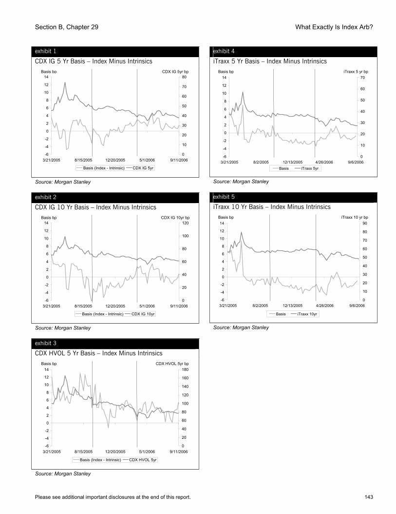
Section B, Chapter 29 What Exactly Is Index Arb?
Please see additional important disclosures at the end of this report. 143
exhibit 1
CDX IG 5 Yr Basis – Index Minus Intrinsics
-6
-4
-2
0
2
4
6
8
10
12
14
3/21/2005 8/15/2005 12/20/2005 5/1/2006 9/11/20060
10
20
30
40
50
60
70
80
Basis (Index - Intrinsic) CDX IG 5yr
Basis bp CDX IG 5yr bp
Source: Morgan Stanley
exhibit 2
CDX IG 10 Yr Basis – Index Minus Intrinsics
-6
-4
-2
0
2
4
6
8
10
12
14
3/21/2005 8/15/2005 12/20/2005 5/1/2006 9/11/20060
20
40
60
80
100
120
Basis (Index - Intrinsic) CDX IG 10yr
Basis bp CDX IG 10yr bp
Source: Morgan Stanley
exhibit 3
CDX HVOL 5 Yr Basis – Index Minus Intrinsics
-6
-4
-2
0
2
4
6
8
10
12
14
3/21/2005 8/15/2005 12/20/2005 5/1/2006 9/11/20060
20
40
60
80
100
120
140
160
180
Basis (Index - Intrinsic) CDX HVOL 5yr
Basis bp CDX HVOL 5yr bp
Source: Morgan Stanley
exhibit 4
iTraxx 5 Yr Basis – Index Minus Intrinsics
-6
-4
-2
0
2
4
6
8
10
12
14
3/21/2005 8/2/2005 12/13/2005 4/26/2006 9/6/20060
10
20
30
40
50
60
70
Basis iTraxx 5yr
Basis bp iTraxx 5 yr bp
Source: Morgan Stanley
exhibit 5
iTraxx 10 Yr Basis – Index Minus Intrinsics
-6
-4
-2
0
2
4
6
8
10
12
14
3/21/2005 8/2/2005 12/13/2005 4/26/2006 9/6/20060
10
20
30
40
50
60
70
80
90
Basis iTraxx 10yr
Basis bp iTraxx 10 yr bp
Source: Morgan Stanley
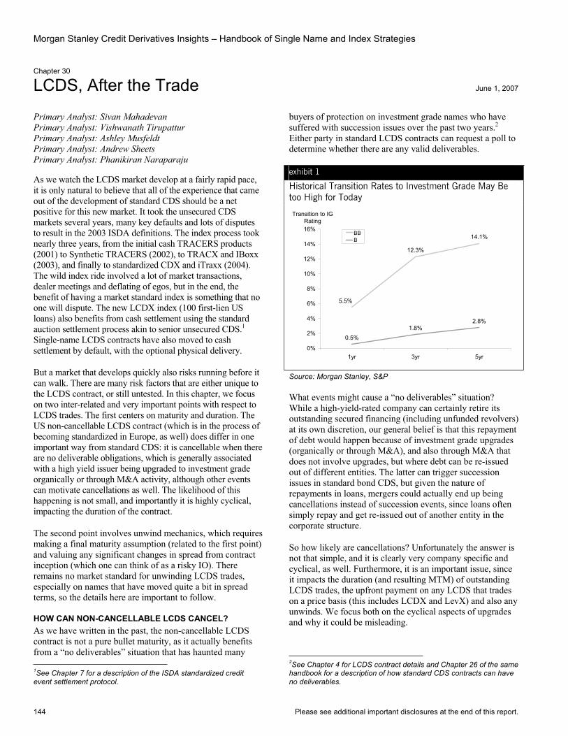
Morgan Stanley Credit Derivatives Insights – Handbook of Single Name and Index Strategies
144 Please see additional important disclosures at the end of this report.
Chapter 30
LCDS, After the Trade June 1, 2007
Primary Analyst: Sivan Mahadevan Primary Analyst: Vishwanath Tirupattur Primary Analyst: Ashley Musfeldt Primary Analyst: Andrew Sheets Primary Analyst: Phanikiran Naraparaju
As we watch the LCDS market develop at a fairly rapid pace, it is only natural to believe that all of the experience that came out of the development of standard CDS should be a net positive for this new market. It took the unsecured CDS markets several years, many key defaults and lots of disputes to result in the 2003 ISDA definitions. The index process took nearly three years, from the initial cash TRACERS products (2001) to Synthetic TRACERS (2002), to TRACX and IBoxx (2003), and finally to standardized CDX and iTraxx (2004). The wild index ride involved a lot of market transactions, dealer meetings and deflating of egos, but in the end, the benefit of having a market standard index is something that no one will dispute. The new LCDX index (100 first-lien US loans) also benefits from cash settlement using the standard auction settlement process akin to senior unsecured CDS.1Single-name LCDS contracts have also moved to cash settlement by default, with the optional physical delivery.
But a market that develops quickly also risks running before it can walk. There are many risk factors that are either unique to the LCDS contract, or still untested. In this chapter, we focus on two inter-related and very important points with respect to LCDS trades. The first centers on maturity and duration. The US non-cancellable LCDS contract (which is in the process of becoming standardized in Europe, as well) does differ in one important way from standard CDS: it is cancellable when there are no deliverable obligations, which is generally associated with a high yield issuer being upgraded to investment grade organically or through M&A activity, although other events can motivate cancellations as well. The likelihood of this happening is not small, and importantly it is highly cyclical, impacting the duration of the contract.
The second point involves unwind mechanics, which requires making a final maturity assumption (related to the first point) and valuing any significant changes in spread from contract inception (which one can think of as a risky IO). There remains no market standard for unwinding LCDS trades, especially on names that have moved quite a bit in spread terms, so the details here are important to follow.
HOW CAN NON-CANCELLABLE LCDS CANCEL? As we have written in the past, the non-cancellable LCDS contract is not a pure bullet maturity, as it actually benefits from a “no deliverables” situation that has haunted many 1See Chapter 7 for a description of the ISDA standardized credit event settlement protocol.
buyers of protection on investment grade names who have suffered with succession issues over the past two years.2Either party in standard LCDS contracts can request a poll to determine whether there are any valid deliverables.
exhibit 1
Historical Transition Rates to Investment Grade May Be too High for Today
12.3%
14.1%
0.5%1.8%
2.8%
5.5%
0%
2%
4%
6%
8%
10%
12%
14%
16%
1yr 3yr 5yr
Transition to IG Rating
BBB
Source: Morgan Stanley, S&P
What events might cause a “no deliverables” situation? While a high-yield-rated company can certainly retire its outstanding secured financing (including unfunded revolvers) at its own discretion, our general belief is that this repayment of debt would happen because of investment grade upgrades (organically or through M&A), and also through M&A that does not involve upgrades, but where debt can be re-issued out of different entities. The latter can trigger succession issues in standard bond CDS, but given the nature of repayments in loans, mergers could actually end up being cancellations instead of succession events, since loans often simply repay and get re-issued out of another entity in the corporate structure.
So how likely are cancellations? Unfortunately the answer is not that simple, and it is clearly very company specific and cyclical, as well. Furthermore, it is an important issue, since it impacts the duration (and resulting MTM) of outstanding LCDS trades, the upfront payment on any LCDS that trades on a price basis (this includes LCDX and LevX) and also any unwinds. We focus both on the cyclical aspects of upgrades and why it could be misleading.
2See Chapter 4 for LCDS contract details and Chapter 26 of the same handbook for a description of how standard CDS contracts can have no deliverables.
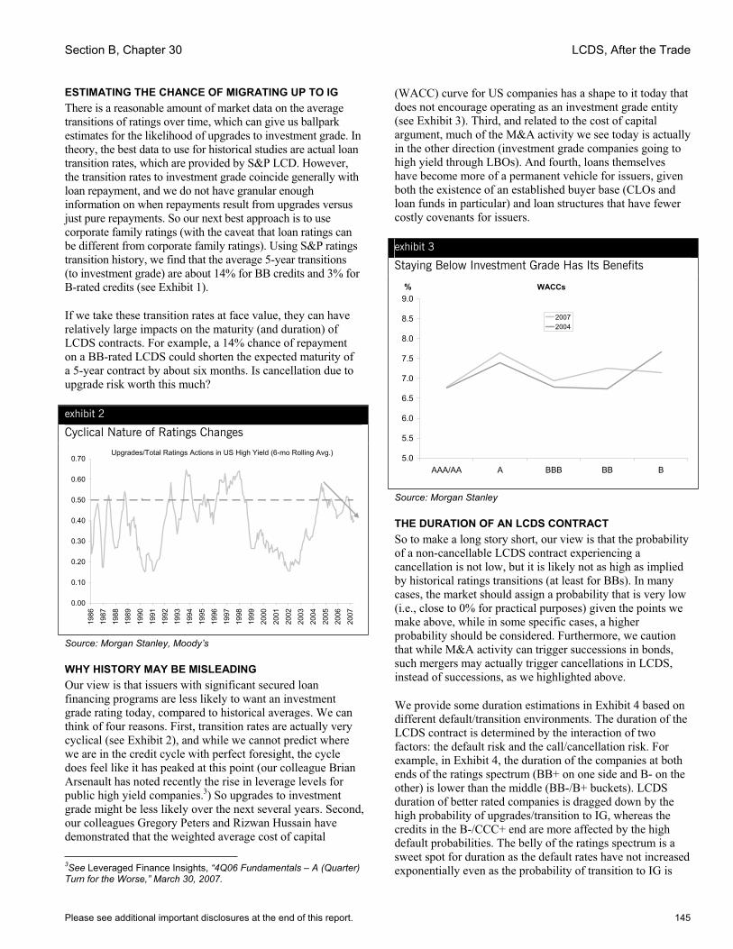
Section B, Chapter 30 LCDS, After the Trade
Please see additional important disclosures at the end of this report. 145
ESTIMATING THE CHANCE OF MIGRATING UP TO IG There is a reasonable amount of market data on the average transitions of ratings over time, which can give us ballpark estimates for the likelihood of upgrades to investment grade. In theory, the best data to use for historical studies are actual loan transition rates, which are provided by S&P LCD. However, the transition rates to investment grade coincide generally with loan repayment, and we do not have granular enough information on when repayments result from upgrades versus just pure repayments. So our next best approach is to use corporate family ratings (with the caveat that loan ratings can be different from corporate family ratings). Using S&P ratings transition history, we find that the average 5-year transitions (to investment grade) are about 14% for BB credits and 3% for B-rated credits (see Exhibit 1).
If we take these transition rates at face value, they can have relatively large impacts on the maturity (and duration) of LCDS contracts. For example, a 14% chance of repayment on a BB-rated LCDS could shorten the expected maturity of a 5-year contract by about six months. Is cancellation due to upgrade risk worth this much?
exhibit 2
Cyclical Nature of Ratings Changes
Upgrades/Total Ratings Actions in US High Yield (6-mo Rolling Avg.)
0.00
0.10
0.20
0.30
0.40
0.50
0.60
0.70
1986
1987
1988
1989
1990
1991
1992
1993
1994
1995
1996
1997
1998
1999
2000
2001
2002
2003
2004
2005
2006
2007
Source: Morgan Stanley, Moody’s
WHY HISTORY MAY BE MISLEADING Our view is that issuers with significant secured loan financing programs are less likely to want an investment grade rating today, compared to historical averages. We can think of four reasons. First, transition rates are actually very cyclical (see Exhibit 2), and while we cannot predict where we are in the credit cycle with perfect foresight, the cycle does feel like it has peaked at this point (our colleague Brian Arsenault has noted recently the rise in leverage levels for public high yield companies.3) So upgrades to investment grade might be less likely over the next several years. Second, our colleagues Gregory Peters and Rizwan Hussain have demonstrated that the weighted average cost of capital 3See Leveraged Finance Insights, “4Q06 Fundamentals – A (Quarter) Turn for the Worse,” March 30, 2007.
(WACC) curve for US companies has a shape to it today that does not encourage operating as an investment grade entity (see Exhibit 3). Third, and related to the cost of capital argument, much of the M&A activity we see today is actually in the other direction (investment grade companies going to high yield through LBOs). And fourth, loans themselves have become more of a permanent vehicle for issuers, given both the existence of an established buyer base (CLOs and loan funds in particular) and loan structures that have fewer costly covenants for issuers.
exhibit 3
Staying Below Investment Grade Has Its Benefits
WACCs
5.0
5.5
6.0
6.5
7.0
7.5
8.0
8.5
9.0
AAA/AA A BBB BB B
%
20072004
Source: Morgan Stanley
THE DURATION OF AN LCDS CONTRACT So to make a long story short, our view is that the probability of a non-cancellable LCDS contract experiencing a cancellation is not low, but it is likely not as high as implied by historical ratings transitions (at least for BBs). In many cases, the market should assign a probability that is very low (i.e., close to 0% for practical purposes) given the points we make above, while in some specific cases, a higher probability should be considered. Furthermore, we caution that while M&A activity can trigger successions in bonds, such mergers may actually trigger cancellations in LCDS, instead of successions, as we highlighted above.
We provide some duration estimations in Exhibit 4 based on different default/transition environments. The duration of the LCDS contract is determined by the interaction of two factors: the default risk and the call/cancellation risk. For example, in Exhibit 4, the duration of the companies at both ends of the ratings spectrum (BB+ on one side and B- on the other) is lower than the middle (BB-/B+ buckets). LCDS duration of better rated companies is dragged down by the high probability of upgrades/transition to IG, whereas the credits in the B-/CCC+ end are more affected by the high default probabilities. The belly of the ratings spectrum is a sweet spot for duration as the default rates have not increased exponentially even as the probability of transition to IG is
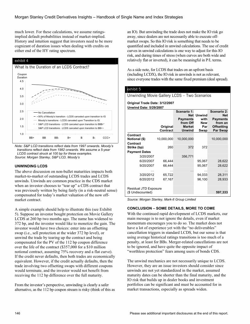
Morgan Stanley Credit Derivatives Insights – Handbook of Single Name and Index Strategies
146 Please see additional important disclosures at the end of this report.
much lower. For these calculations, we assume ratings-implied default probabilities instead of market-implied. History and intuition suggest that investors need to be more cognizant of duration issues when dealing with credits on either end of the HY rating spectrum.
exhibit 4
What Is the Duration of an LCDS Contract?
1.0
1.5
2.0
2.5
3.0
3.5
4.0
4.5
BB+ BB BB- B+ B B- CCC+
Coupon Duration
No Cancellation 50% of Moody's transition - LCDS canceled upon transition to IGMoody's transitions - LCDS canceled upon Transition to IGS&P LCD transitions - LCDS canceled upon transition to BBB-*S&P LCD transitions - LCDS canceled upon transition to BB+~
Note: S&P LCD transitions reflect data from 1997 onwards. Moody’s transitions reflect data from 1982 onwards. We assume a 5-year LCDS contract struck at 100 bp for these examples.
Source: Morgan Stanley, S&P LCD, Moody’s
UNWINDING LCDS The above discussion on non-bullet maturities impacts both market-to-market of outstanding LCDS trades and LCDS unwinds. Unwinds are common practice in the CDS market when an investor chooses to “tear up” a CDS contract that was previously written by being fairly (in a risk-neutral sense) compensated for today’s market valuation of the now off-market contract.
A simple example should help to illustrate this (see Exhibit 5). Suppose an investor bought protection on Movie Gallery LCDS at 260 bp two months ago. The name has widened to 372 bp, and the investor would like to monetize the gain. The investor would have two choices: enter into an offsetting swap (i.e., sell protection at the wider 372 bp level), or unwind the trade by tearing up the contract and being compensated for the PV of the 112 bp coupon difference over the life of the contract ($357,000 for a $10 million notional contract, assuming 75% recovery and a flat curve). If the credit never defaults, then both trades are economically equivalent. However, if the credit actually defaults, then the trade involving two offsetting swaps with different coupons would terminate, and the investor would not benefit from receiving the 112 bp difference over the full maturity.
From the investor’s perspective, unwinding is clearly a safer alternative, as the 112 bp coupon stream is risky (think of this as
an IO). But unwinding the trade does not make the IO risk go away, since dealers are not necessarily able to execute off-market swaps. So this IO risk is something that needs to be quantified and included in unwind calculations. The use of credit curves in unwind calculations is one way to adjust for this IO risk, and during times of stress (when curves are both wide and relatively flat or inverted), it can be meaningful in P/L terms.
As a side note, for LCDS that trades on an upfront basis (including LCDX), the IO risk in unwinds is not as relevant, since everyone trades with the same fixed premium (deal spread).
exhibit 5
Unwinding Movie Gallery LCDS – Two Scenarios
Original Trade Date: 3/12/2007Unwind Date: 5/29/2007
Original Contract
Scenario 1: Net
Payments from Off
MarketUnwind
Unwind with New Par
Swap
Scenario 2: Net
Payments from an
Offsetting Par Swap
Contract Notional ($) 10,000,000 10,000,000 10,000,000Contract Strike (bp) 260 372 372Payment Dates
3/20/2007 356,7716/20/2007 66,444 95,067 28,6229/20/2007 66,444 95,067 28,622
… … … … …3/20/2012 65,722 94,033 28,3116/20/2012 67,167 96,100 28,933
Residual JTD Exposure($ Undiscounted) 597,333
Source: Morgan Stanley, Mark-It Group Limited
CONCLUSION – SOME DETAILS, MORE TO COME With the continued rapid development of LCDS markets, our main message is to not ignore the details, even if market momentum encourages you to do so. The market does not have a lot of experience yet with the “no deliverables”cancellation triggers in standard LCDS, but our sense is that using average historical ratings transitions is too much of a penalty, at least for BBs. Merger-related cancellations are not to be ignored, and have quite the opposite impact of “worthless protection” fears among users of bonds CDS.
The unwind mechanics are not necessarily unique to LCDS. However, they are an issue investors should consider since unwinds are not yet standardized in the market, assumed maturity dates can be shorter than the final maturity, and the IO risk that builds up in dealer books and investment portfolios can be significant and must be accounted for in market transactions, especially as spreads widen.
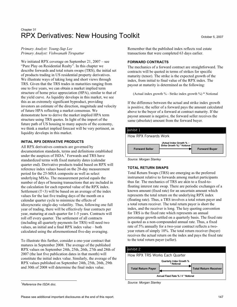
Please see additional important disclosures at the end of this report. 147
Chapter 31
RPX Derivatives: New Housing Toolkit October 5, 2007
Primary Analyst: Young-Sup Lee Primary Analyst: Vishwanath Tirupattur
We initiated RPX coverage on September 21, 2007 – see “Pure Play on Residential Realty”. In this chapter we describe forwards and total return swaps (TRS), the initial set of products trading in US residential property derivatives. We illustrate ways of taking long and short views through TRS. Given that the TRS trades in maturities ranging from one to five years, we can obtain a market implied term structure of home price appreciation (HPA), similar to that of the yield curve. As liquidity develops in this market, we see this as an extremely significant byproduct, providing investors an estimate of the direction, magnitude and velocity of future HPA reflecting a market consensus. We demonstrate how to derive the market implied HPA term structure using TRS quotes. In light of the import of the future path of US housing to many aspects of the economy, we think a market implied forecast will be very pertinent, as liquidity develops in this market.
INITIAL RPX DERIVATIVE PRODUCTS All RPX derivatives contracts are governed by documentation standards, terms and definitions established under the auspices of ISDA.1 Forwards and TRS have standardized terms with fixed maturity dates (calendar quarter end). Derivative products traded based on RPX will reference index values based on the 28-day measurement period for the 25-MSA composite as well as select underlying MSAs. The measurement period equals the number of days of housing transactions that are included in the calculation for each reported value of the RPX index. Settlement (T+3) will be based on an average of the index values for the last five trading days of the month on a calendar quarter cycle to minimize the effects of idiosyncratic single-day volatility. Thus, following one full year of trading, there will be effectively four contracts per year, maturing at each quarter for 1-5 years. Contracts will roll off every quarter. The settlement of all contracts (including all quarterly payments for TRS) will need two values, an initial and a final RPX index value – both calculated using the aforementioned five-day averaging.
To illustrate this further, consider a one-year contract that matures in September 2008. The average of the published RPX values on September 24th, 25th, 26th, 27th and 28th of 2007 (the last five publication dates in that month) will constitute the initial index value. Similarly, the average of the RPX values published on September 24th, 25th, 26th, 29th and 30th of 2008 will determine the final index value.
1Reference the ISDA doc.
Remember that the published index reflects real estate transactions that were completed 63 days earlier.
FORWARD CONTRACTS The mechanics of a forward contract are straightforward. The contracts will be quoted in terms of strikes for specific maturity (tenor). The strike is the expected growth of the index, from initial to final value of the RPX index. The payout at maturity is determined as the following:
(Actual index growth % - Strike index growth %) * Notional
If the difference between the actual and strike index growth is positive, the seller of a forward pays the amount calculated above to the buyer of a forward at contract maturity. If the payout amount is negative, the forward seller receives the same (absolute) amount from the forward buyer.
exhibit 1
How RPX Forwards Work
(Actual Index Growth % –Strike Growth %) * Notional
Forward Seller Forward Buyer
(Actual Index Growth % –Strike Growth %) * Notional
Forward Seller Forward Buyer
Source: Morgan Stanley
TOTAL RETURN SWAPS Total Return Swaps (TRS) are emerging as the preferred instrument relative to forwards among market participants thus far. The mechanics of TRS are akin to a fixed-to-floating interest rate swap. There are periodic exchanges of a known amount (fixed rate) for an uncertain amount which represents the total return on the underlying RPX index (floating rate). Thus, a TRS involves a total return payer and a total return receiver. The total return payer is short the index, and the receiver is long. The key quoting convention for TRS is the fixed rate which represents an annual percentage growth settled on a quarterly basis. The fixed rate is quoted as a non-compounded annual rate. Thus, a fixed rate of 5% annually for a two-year contract reflects a two-year return of simply 10%. The total return receiver (buyer) receives the actual return on the index and pays the fixed rate to the total return payer (seller).
exhibit 2
How RPX TRS Works Each Quarter Quarterly Index Growth %
* Notional
Annual Fixed Rate % / 4 * Notional
Total Return Payer Total Return Receiver
Quarterly Index Growth %* Notional
Annual Fixed Rate % / 4 * Notional
Total Return Payer Total Return Receiver
Source: Morgan Stanley
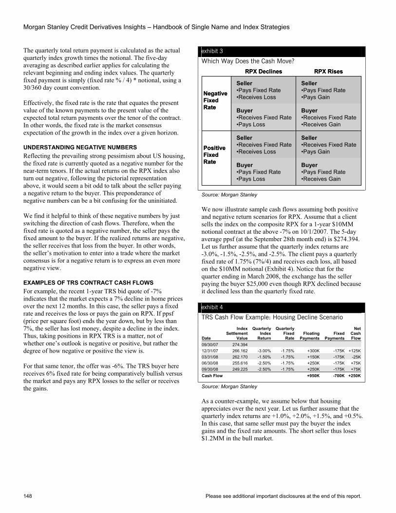
Morgan Stanley Credit Derivatives Insights – Handbook of Single Name and Index Strategies
148 Please see additional important disclosures at the end of this report.
The quarterly total return payment is calculated as the actual quarterly index growth times the notional. The five-day averaging as described earlier applies for calculating the relevant beginning and ending index values. The quarterly fixed payment is simply (fixed rate % / 4) * notional, using a 30/360 day count convention.
Effectively, the fixed rate is the rate that equates the present value of the known payments to the present value of the expected total return payments over the tenor of the contract. In other words, the fixed rate is the market consensus expectation of the growth in the index over a given horizon.
UNDERSTANDING NEGATIVE NUMBERS Reflecting the prevailing strong pessimism about US housing, the fixed rate is currently quoted as a negative number for the near-term tenors. If the actual returns on the RPX index also turn out negative, following the pictorial representation above, it would seem a bit odd to talk about the seller paying a negative return to the buyer. This preponderance of negative numbers can be a bit confusing for the uninitiated.
We find it helpful to think of these negative numbers by just switching the direction of cash flows. Therefore, when the fixed rate is quoted as a negative number, the seller pays the fixed amount to the buyer. If the realized returns are negative, the seller receives that loss from the buyer. In other words, the seller’s motivation to enter into a trade where the market consensus is for a negative return is to express an even more negative view.
EXAMPLES OF TRS CONTRACT CASH FLOWS For example, the recent 1-year TRS bid quote of -7% indicates that the market expects a 7% decline in home prices over the next 12 months. In this case, the seller pays a fixed rate and receives the loss or pays the gain on RPX. If ppsf (price per square foot) ends the year down, but by less than 7%, the seller has lost money, despite a decline in the index. Thus, taking positions in RPX TRS is a matter, not of whether one’s outlook is negative or positive, but rather the degree of how negative or positive the view is.
For that same tenor, the offer was -6%. The TRS buyer here receives 6% fixed rate for being comparatively bullish versus the market and pays any RPX losses to the seller or receives the gains.
exhibit 3
Which Way Does the Cash Move?
Seller•Receives Fixed Rate•Pays Gain
Seller•Receives Fixed Rate•Receives Loss
Seller•Pays Fixed Rate•Pays Gain
Seller•Pays Fixed Rate•Receives Loss
RPX RisesRPX Declines
PositiveFixedRate
NegativeFixedRate
Buyer•Pays Fixed Rate•Receives Gain
Buyer•Pays Fixed Rate•Pays Loss
Buyer•Receives Fixed Rate•Receives Gain
Buyer•Receives Fixed Rate•Pays Loss
Source: Morgan Stanley
We now illustrate sample cash flows assuming both positive and negative return scenarios for RPX. Assume that a client sells the index on the composite RPX for a 1-year $10MM notional contract at the above -7% on 10/1/2007. The 5-day average ppsf (at the September 28th month end) is $274.394. Let us further assume that the quarterly index returns are -3.0%, -1.5%, -2.5%, and -2.5%. The client pays a quarterly fixed rate of 1.75% (7%/4) and receives each loss, all based on the $10MM notional (Exhibit 4). Notice that for the quarter ending in March 2008, the exchange has the seller paying the buyer $25,000 even though RPX declined because it declined less than the quarterly fixed rate.
exhibit 4
TRS Cash Flow Example: Housing Decline Scenario
Date
IndexSettlement
Value
Quarterly Index
Return
Quarterly FixedRate
FloatingPayments
FixedPayments
NetCashFlow
09/30/07 274.39412/31/07 266.162 -3.00% -1.75% +300K -175K +125K03/31/08 262.170 -1.50% -1.75% +150K -175K -25K06/30/08 255.616 -2.50% -1.75% +250K -175K +75K09/30/08 249.225 -2.50% -1.75% +250K -175K +75KCash Flow +950K -700K +250K
Source: Morgan Stanley
As a counter-example, we assume below that housing appreciates over the next year. Let us further assume that the quarterly index returns are +1.0%, +2.0%, +1.5%, and +0.5%. In this case, that same seller must pay the buyer the index gains and the fixed rate amounts. The short seller thus loses $1.2MM in the bull market.

Section B, Chapter 31 RPX Derivatives: New Housing Toolkit
Please see additional important disclosures at the end of this report. 149
exhibit 5
TRS Cash Flow Example: Housing Gain Scenario
Date
IndexSettlement
Value
Quarterly Index
Return
Quarterly FixedRate
FloatingPayments
FixedPayments
NetCashFlow
09/30/07 274.394 12/31/07 277.138 1.00% -1.75% -100K -175K -275K03/31/08 282.681 2.00% -1.75% -200K -175K -375K06/30/08 286.921 1.50% -1.75% -150K -175K -325K09/30/08 288.356 0.50% -1.75% -50K -175K -225KCash Flow -500K -700K -1200K
Source: Morgan Stanley
TERM STRUCTURE OF HOME PRICES Much like the cash bond market, the pricing of multiple tenors (maturities) can be used to estimate the implied forward rates. Radar Logic publishes daily mid-market closing levels (1-5 year TRS) using a dealer poll on each trading day for the RPX 25-MSA composite index. We show the market implied term structure of HPA using the fixings as of October 3, 2007.
exhibit 6
TRS Official Fixings
Date 1-year 2-year 3-year 4-year 5-year10/03/07 -6.38% -4.78% -3.69% -1.69% -0.44%
Source: Radar Logic
The one-year expectation is simply that contract’s fixed rate, -6.4%. Since the rates are additive, not compounded, from year to year, it is clear that the second year’s loss is not as dramatic. The two-year contract level of -4.8% implies a total loss of 9.6% over the two-year period. Thus, the second year’s incremental loss is only 3.2%. Continuing with this recursion, we see forward gains in the 4th year. Thus, the market is implying a rebound in HPA sometime in 2011. RPX TRS offers opportunities to make bets on quicker or slower rebound.
This analysis is meant to be illustrative. We have made a few simplifying assumptions which are worth pointing out. We have ignored the quarterly nature of cash flows and related compounding. For longer tenors, this could be meaningful. Further, the quarterly settlement also implies path dependency for cash flows. High intra-year volatility in the index will result in forward curves significantly different than the simplified approach above suggests.
As an example of a forward-looking bet with RPX TRS, we look at a long year-3 bet: an investor buys 3-year TRS and sells 2-year TRS. Using the quotes from Exhibit 6, for the first two years, this investor would pay 4.78% and receive 3.69% for a net outlay of 1.09% each year, or a total of 2.18% of the notional. During the first two years, there is no net exposure to RPX. In the third year, however, the investor receives the 3.69% fixed rate. Subtracting the 2.18% (nominal) outlay of the first two years, this leaves a net inflow of 1.51%. The investor is long the index in the third year. Neglecting the borrowing expense of the first 2-year outlays, this means that the investor can withstand a loss of
1.51% and still break even. Investors who believe that housing will rebound sooner than the market implies can benefit from such a curve trade in RPX TRS. Similar trades can occur for a variety of forward periods. Remember that bid/offer would increase that breakeven.
exhibit 7
Four Years to a Rebound
-12%
-10%
-8%
-6%
-4%
-2%
0%
2%
4%
6%
1 2 3 4 5
Years
Mid-Market Quote Cumulative Return Forward Return
Source: Radar Logic, Morgan Stanley
EYE ON CITIES As continued evidence of the growing interest in RPX, this week marks the start of trading quotes on MSA level 1-year contracts. While only three cities (New York, Los Angeles and Miami) receive this distinction (and at wider-than-composite bid/offers), we do note that New York and Los Angeles are the two largest MSAs in the RPX composite. Along with Miami, this trio accounts for 44% of index weight and 34% of the covered population.2
The ppsf of this group is 18% higher than the composite. Historically, the group has experienced a 95% correlation to the 25-MSA composite suggesting potential for long/short trading strategies. Initial indications for one-year HPA are negative for all three cities (Miami -15.5%, Los Angeles -9.5% and New York, -1.5%), based on mid-market expectations. Given our quest for geographical specificity, we will keep a watchful eye on these (and hopefully more) MSAs.
CONCLUSIONEncouraged by the increasing focus, tightening bid/offer, and the expansion of the US residential property derivatives market into the MSA level, we continue our discussions into the new tool kit for investors made possible through residential property derivatives market. Forestalling the credit crunch intensifying the correction in housing was a major motivation for the Fed cutting rates on September 18, 2007. In the current state of the US economy, the housing market is seen as a key risk and anticipation of further deterioration is widespread from many quarters ranging from market participants to policy makers. As such, the market implied estimates of the timing, magnitude and velocity of HPA provide a good point of reference. 2The three cities account for 16% of US population. The 25 MSAs cover almost half the country.
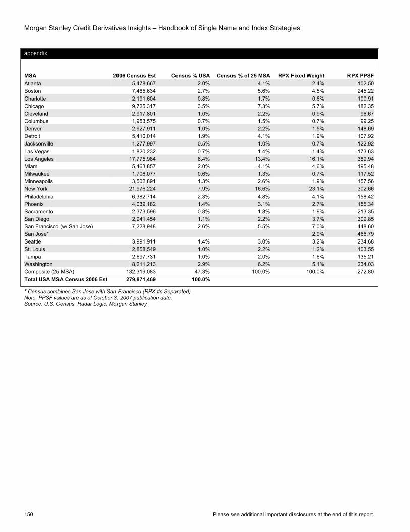
Morgan Stanley Credit Derivatives Insights – Handbook of Single Name and Index Strategies
150 Please see additional important disclosures at the end of this report.
appendix
MSA 2006 Census Est Census % USA Census % of 25 MSA RPX Fixed Weight RPX PPSFAtlanta 5,478,667 2.0% 4.1% 2.4% 102.50Boston 7,465,634 2.7% 5.6% 4.5% 245.22Charlotte 2,191,604 0.8% 1.7% 0.6% 100.91Chicago 9,725,317 3.5% 7.3% 5.7% 182.35Cleveland 2,917,801 1.0% 2.2% 0.9% 96.67Columbus 1,953,575 0.7% 1.5% 0.7% 99.25Denver 2,927,911 1.0% 2.2% 1.5% 148.69Detroit 5,410,014 1.9% 4.1% 1.9% 107.92Jacksonville 1,277,997 0.5% 1.0% 0.7% 122.92Las Vegas 1,820,232 0.7% 1.4% 1.4% 173.63Los Angeles 17,775,984 6.4% 13.4% 16.1% 389.94Miami 5,463,857 2.0% 4.1% 4.6% 195.48Milwaukee 1,706,077 0.6% 1.3% 0.7% 117.52Minneapolis 3,502,891 1.3% 2.6% 1.9% 157.56New York 21,976,224 7.9% 16.6% 23.1% 302.66Philadelphia 6,382,714 2.3% 4.8% 4.1% 158.42Phoenix 4,039,182 1.4% 3.1% 2.7% 155.34Sacramento 2,373,596 0.8% 1.8% 1.9% 213.35San Diego 2,941,454 1.1% 2.2% 3.7% 309.85San Francisco (w/ San Jose) 7,228,948 2.6% 5.5% 7.0% 448.60San Jose* 2.9% 466.79Seattle 3,991,911 1.4% 3.0% 3.2% 234.68St. Louis 2,858,549 1.0% 2.2% 1.2% 103.55Tampa 2,697,731 1.0% 2.0% 1.6% 135.21Washington 8,211,213 2.9% 6.2% 5.1% 234.03Composite (25 MSA) 132,319,083 47.3% 100.0% 100.0% 272.80Total USA MSA Census 2006 Est 279,871,469 100.0%
* Census combines San Jose with San Francisco (RPX #s Separated) Note: PPSF values are as of October 3, 2007 publication date. Source: U.S. Census, Radar Logic, Morgan Stanley
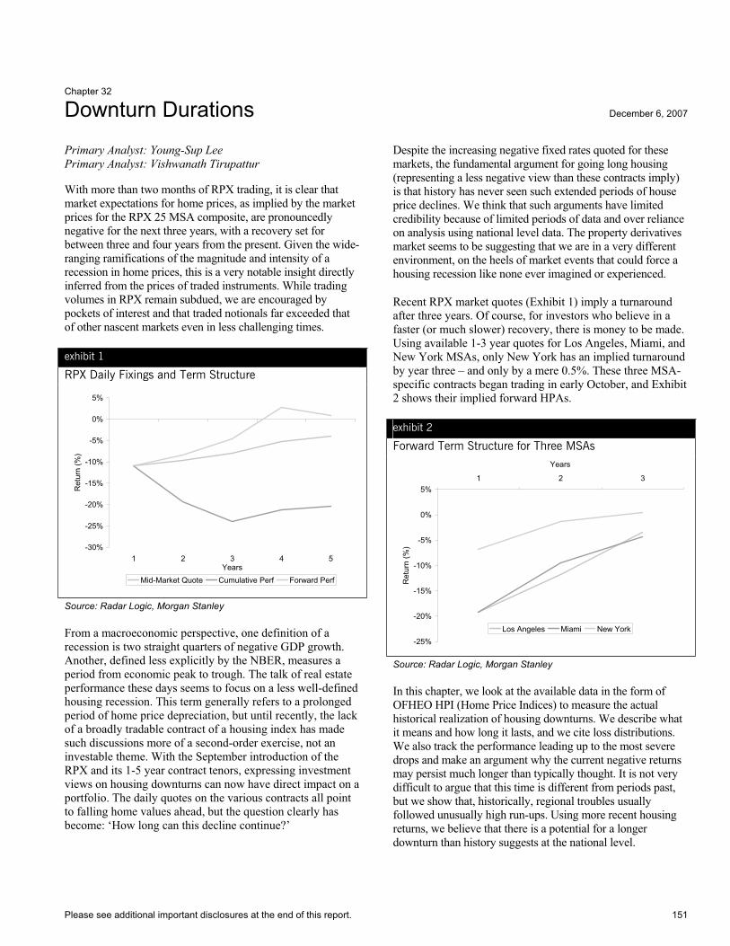
Please see additional important disclosures at the end of this report. 151
Chapter 32
Downturn Durations December 6, 2007
Primary Analyst: Young-Sup Lee Primary Analyst: Vishwanath Tirupattur
With more than two months of RPX trading, it is clear that market expectations for home prices, as implied by the market prices for the RPX 25 MSA composite, are pronouncedly negative for the next three years, with a recovery set for between three and four years from the present. Given the wide-ranging ramifications of the magnitude and intensity of a recession in home prices, this is a very notable insight directly inferred from the prices of traded instruments. While trading volumes in RPX remain subdued, we are encouraged by pockets of interest and that traded notionals far exceeded that of other nascent markets even in less challenging times.
exhibit 1
RPX Daily Fixings and Term Structure
-30%
-25%
-20%
-15%
-10%
-5%
0%
5%
1 2 3 4 5Years
Ret
urn
(%)
Mid-Market Quote Cumulative Perf Forward Perf
Source: Radar Logic, Morgan Stanley
From a macroeconomic perspective, one definition of a recession is two straight quarters of negative GDP growth. Another, defined less explicitly by the NBER, measures a period from economic peak to trough. The talk of real estate performance these days seems to focus on a less well-defined housing recession. This term generally refers to a prolonged period of home price depreciation, but until recently, the lack of a broadly tradable contract of a housing index has made such discussions more of a second-order exercise, not an investable theme. With the September introduction of the RPX and its 1-5 year contract tenors, expressing investment views on housing downturns can now have direct impact on a portfolio. The daily quotes on the various contracts all point to falling home values ahead, but the question clearly has become: ‘How long can this decline continue?’
Despite the increasing negative fixed rates quoted for these markets, the fundamental argument for going long housing (representing a less negative view than these contracts imply) is that history has never seen such extended periods of house price declines. We think that such arguments have limited credibility because of limited periods of data and over reliance on analysis using national level data. The property derivatives market seems to be suggesting that we are in a very different environment, on the heels of market events that could force a housing recession like none ever imagined or experienced.
Recent RPX market quotes (Exhibit 1) imply a turnaround after three years. Of course, for investors who believe in a faster (or much slower) recovery, there is money to be made. Using available 1-3 year quotes for Los Angeles, Miami, and New York MSAs, only New York has an implied turnaround by year three – and only by a mere 0.5%. These three MSA-specific contracts began trading in early October, and Exhibit 2 shows their implied forward HPAs.
exhibit 2
Forward Term Structure for Three MSAs
-25%
-20%
-15%
-10%
-5%
0%
5%1 2 3
Years
Ret
urn
(%)
Los Angeles Miami New York
Source: Radar Logic, Morgan Stanley
In this chapter, we look at the available data in the form of OFHEO HPI (Home Price Indices) to measure the actual historical realization of housing downturns. We describe what it means and how long it lasts, and we cite loss distributions. We also track the performance leading up to the most severe drops and make an argument why the current negative returns may persist much longer than typically thought. It is not very difficult to argue that this time is different from periods past, but we show that, historically, regional troubles usually followed unusually high run-ups. Using more recent housing returns, we believe that there is a potential for a longer downturn than history suggests at the national level.

Morgan Stanley Credit Derivatives Insights – Handbook of Single Name and Index Strategies
152 Please see additional important disclosures at the end of this report.
THE DATA Our choice to use OFHEO data is simply to get as long a history as possible. RPX only has data since 2000, so it would only measure through a single economic recession. Although the HPI only includes houses backed by conforming (i.e., smaller) mortgages, we believe that any relevant impacts of prolonged underperformance can be felt in this segment of the marketplace. To narrow the focus, we look only at the 25 MSAs (metropolitan statistical areas) that are also covered by RPX. These cities represent about 44% of the nation’s population. Despite OFHEO’s quarterly releases, we concentrate on full annual returns to minimize any seasonal effects in the analysis. The largest time series across all areas begins in 1979, and we consider only full-year returns through 2006.
THE DISTRIBUTION Interestingly enough, the OFHEO national composite index has never had a negative return year. This may in part be due to the lower volatility of conforming home loans, but we do not see this as a major drawback (to be explained later). We knew going in that negative return observations would be few and far between (if any, and in this case none). Bear in mind our original point: it is the lack of historical downturns which investors are using to argue that things could not be as bad as the market implies. We want to dig deeper into the available data to uncover the not so obvious. By looking at the individual MSA numbers, we know that regional downturns happen about 11% of the time (80 out of a possible 700 MSA-years). This is highlighted in Exhibit 3. The average negative streak lasts 1.5 years (80 MSA-years over 53 observations).
exhibit 3
Distribution of Downturns
Streak Length (Yrs) # Observations # Included Yrs # MSAs1 41 41 142 5 10 43 2 6 24 2 8 25 3 15 3Total 53 80 25
Source: OFHEO, Morgan Stanley
However, there were seven instances of 3+ consecutive years of home price losses out of 53 episodes of downturns (13%), which does not appear to be such a small frequency to us. As Exhibit 4 shows, in every case, the previous 3 years to that streak were marked by very strong gains. Boston in 1989-1992 is the only case where the previous three years did not beat the positive years’ average for the same time period (yet it still returned 37% during 1986-1988). The other examples show prior 3-year performance in the 40-70% range.
exhibit 4
The Worst of the Worst
MSA Streak Length
(Yrs) YearsTotal Loss
(%)Prior 3-Yrs
(%)New York 3 89-91 -7.4 51.7Sacramento 3 92-94 -12.9 42.0Boston 4 89-92 -11.3 36.5San Diego 4 91-94 -9.7 41.9San Francisco 5 90-94 -11.0 72.3San Jose 5 90-94 -12.7 74.1Los Angeles 5 90-94 -19.4 71.3
Source: OFHEO, Morgan Stanley
To strengthen our case, Exhibit 5 shows a scatter plot of all downturn streaks. Note the strong correlation (-46%) between the size and duration of the losses versus the prior 3-year performance. We would argue that since the most recent composite performance is 34% (OFHEO 3-year ending in 2006), there is a stronger likelihood that any downturn (which we are already experiencing) could last longer than “typical” declines. Because of the higher perceived correlation of the different regions due to more universal themes, we believe in less “diversification” effects this time around.
exhibit 5
Downturns and Prior Run-Ups
Downturns and Prior Run-ups
-20
-10
0
10
20
30
40
50
60
70
80
-25.00 -20.00 -15.00 -10.00 -5.00 0.00Negative Streak Return (%)
Prio
r 3-Y
ears
Ret
urn
(%)
1 streak2 streak3 streak4 streak5 streak
Source: OFHEO, Morgan Stanley
For those who are still convinced that OFHEO HPI is not representative of the market at large, we repeat our original distribution, but this time on returns that are one standard deviation below the historical average for each MSA. In this case, the number of observed below-average streaks rises to 83, but the concentration is more focused on shorter streaks. The average length is still about 1.5 years, so even liberal interpretations of housing downturns do not dramatically change the aggregate results much.

Section B, Chapter 32 Downturn Durations
Please see additional important disclosures at the end of this report. 153
CONCLUSIONWe see that 16 of the 25 MSAs have had recent 3-year returns (2004-2006) higher than is typical; we also see this for the national composite (at close to double its 3-year average). We notice that in 23 cases, the 2006 return is slowing versus 2004-05; this may also be an indication of a pronounced downturn. Subprime delinquencies for the 2006-07 vintages remain at levels much higher than for any previous vintage — and a large chunk of them will lead to foreclosures, and forced liquidations, which we expect to put further pressure on home prices. Further, the rising supply of
homes, falling home sales, declining consumer confidence and widening jumbo-conforming mortgage rate spreads all point to more broad-based housing price pressures this time around. The recent trend of more negative TRS levels across all contracts confirms our belief that the downturn can be with us for a while. Yes, there is always a chance that things can change quickly, but given the tremendous overhang of subprime pressures, risk of recession, and the higher cross-regional correlations, we think the probability of a 3+ year downturn is substantial. We believe that the regional behaviors of the past can serve as guides on a larger scale.


Section C
Basis Ideas
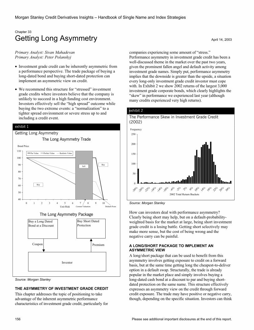
Morgan Stanley Credit Derivatives Insights – Handbook of Single Name and Index Strategies
156 Please see additional important disclosures at the end of this report.
Chapter 33
Getting Long Asymmetry April 14, 2003
Primary Analyst: Sivan Mahadevan Primary Analyst: Peter Polanskyj
• Investment grade credit can be inherently asymmetric from a performance perspective. The trade package of buying a long-dated bond and buying short-dated protection can implement an asymmetric view on credit.
• We recommend this structure for “stressed” investment grade credits where investors believe that the company is unlikely to succeed in a high funding cost environment. Investors effectively sell the “high spread” outcome while buying the two extreme events: a “normalization” to a tighter spread environment or severe stress up to and including a credit event.
exhibit 1
Getting Long Asymmetry
The Long Asymmetry Trade
Bond Price
40
50
60
70
80
90
100
110
0 1 2 3 4 5 6 7 8 9 10Unit Risk
Par Value Perfect Value Realistic Value
Buy
Buy
Default Point
Sell
Current Valuation
The Long Asymmetry Package
Investor
Buy a Long Dated Bond at a Discount
Buy Short Dated Protection
Coupon Premium
Source: Morgan Stanley
THE ASYMMETRY OF INVESTMENT GRADE CREDIT This chapter addresses the topic of positioning to take advantage of the inherent asymmetric performance characteristics of investment grade credit, particularly for
companies experiencing some amount of “stress.” Performance asymmetry in investment grade credit has been a well-discussed theme in the market over the past two years, given the prominent fallen angel and default activity among investment grade names. Simply put, performance asymmetry implies that the downside is greater than the upside, a situation every long-only investment grade credit investor must cope with. In Exhibit 2 we show 2002 returns of the largest 3,000 investment grade corporate bonds, which clearly highlights the “skew” in performance we experienced last year (although many credits experienced very high returns).
exhibit 2
The Performance Skew in Investment Grade Credit (2002)
Frequency
0
50
100
150
200
250
-30%
-26%
-22%
-18%
-14%
-10% -6% -2% 2% 6% 10
%14
%18
%22
%26
%30
%
2002 Total Return Buckets
Source: Morgan Stanley
How can investors deal with performance asymmetry? Clearly being short may help, but on a default-probability-weighted basis for the market at large, being short investment grade credit is a losing battle. Getting short selectively may make more sense, but the cost of being wrong and the negative carry can be painful.
A LONG/SHORT PACKAGE TO IMPLEMENT AN ASYMMETRIC VIEW A long/short package that can be used to benefit from this asymmetry involves getting exposure to credit on a forward basis, but at the same time getting long the cheapest-to-deliver option in a default swap. Structurally, the trade is already popular in the market place and simply involves buying a long-dated cash bond at a discount to par and buying short-dated protection on the same name. This structure effectively expresses an asymmetry view on the credit through forward credit exposure. The trade may have positive or negative carry, though, depending on the specific situation. Investors can think
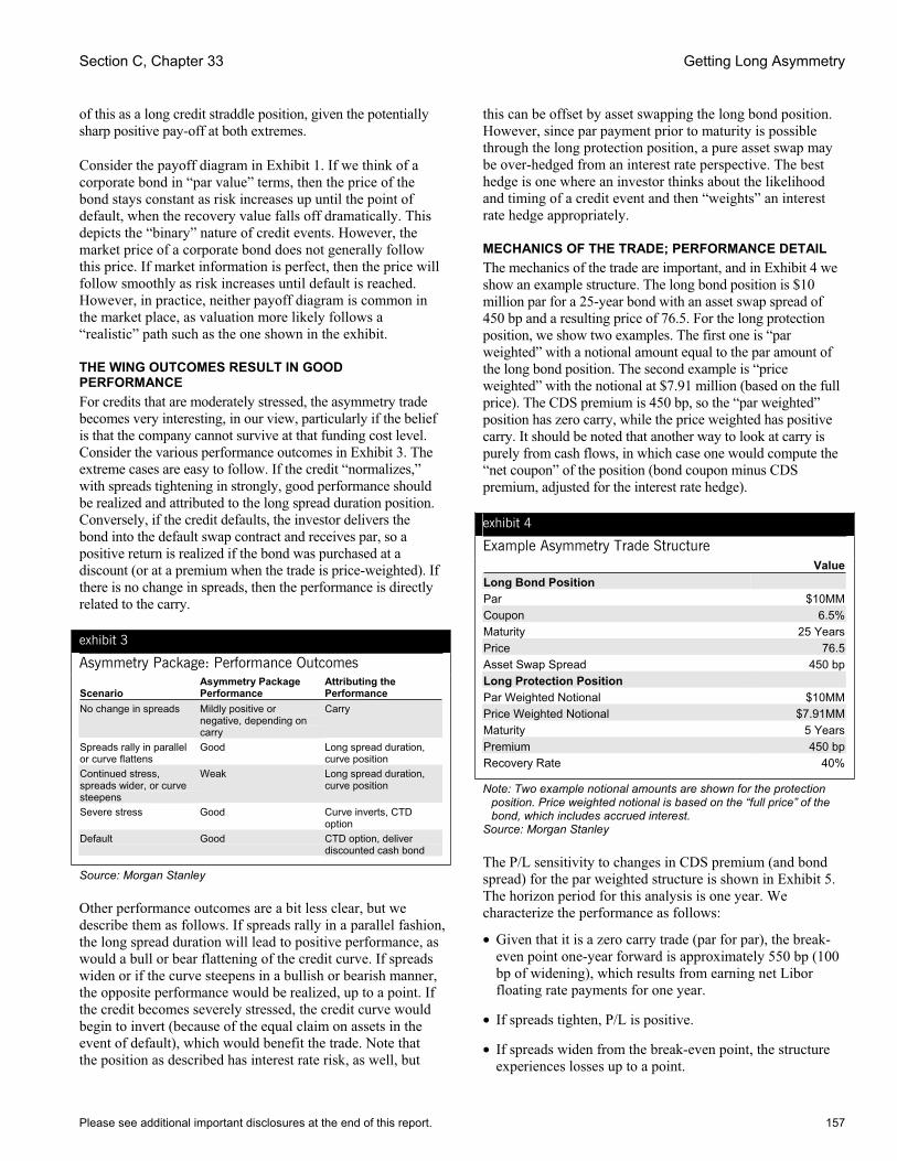
Section C, Chapter 33 Getting Long Asymmetry
Please see additional important disclosures at the end of this report. 157
of this as a long credit straddle position, given the potentially sharp positive pay-off at both extremes.
Consider the payoff diagram in Exhibit 1. If we think of a corporate bond in “par value” terms, then the price of the bond stays constant as risk increases up until the point of default, when the recovery value falls off dramatically. This depicts the “binary” nature of credit events. However, the market price of a corporate bond does not generally follow this price. If market information is perfect, then the price will follow smoothly as risk increases until default is reached. However, in practice, neither payoff diagram is common in the market place, as valuation more likely follows a “realistic” path such as the one shown in the exhibit.
THE WING OUTCOMES RESULT IN GOOD PERFORMANCE For credits that are moderately stressed, the asymmetry trade becomes very interesting, in our view, particularly if the belief is that the company cannot survive at that funding cost level. Consider the various performance outcomes in Exhibit 3. The extreme cases are easy to follow. If the credit “normalizes,” with spreads tightening in strongly, good performance should be realized and attributed to the long spread duration position. Conversely, if the credit defaults, the investor delivers the bond into the default swap contract and receives par, so a positive return is realized if the bond was purchased at a discount (or at a premium when the trade is price-weighted). If there is no change in spreads, then the performance is directly related to the carry.
exhibit 3
Asymmetry Package: Performance Outcomes
ScenarioAsymmetry Package Performance
Attributing the Performance
No change in spreads Mildly positive or negative, depending on carry
Carry
Spreads rally in parallel or curve flattens
Good Long spread duration, curve position
Continued stress, spreads wider, or curve steepens
Weak Long spread duration, curve position
Severe stress Good Curve inverts, CTD option
Default Good CTD option, deliver discounted cash bond
Source: Morgan Stanley
Other performance outcomes are a bit less clear, but we describe them as follows. If spreads rally in a parallel fashion, the long spread duration will lead to positive performance, as would a bull or bear flattening of the credit curve. If spreads widen or if the curve steepens in a bullish or bearish manner, the opposite performance would be realized, up to a point. If the credit becomes severely stressed, the credit curve would begin to invert (because of the equal claim on assets in the event of default), which would benefit the trade. Note that the position as described has interest rate risk, as well, but
this can be offset by asset swapping the long bond position. However, since par payment prior to maturity is possible through the long protection position, a pure asset swap may be over-hedged from an interest rate perspective. The best hedge is one where an investor thinks about the likelihood and timing of a credit event and then “weights” an interest rate hedge appropriately.
MECHANICS OF THE TRADE; PERFORMANCE DETAIL The mechanics of the trade are important, and in Exhibit 4 we show an example structure. The long bond position is $10 million par for a 25-year bond with an asset swap spread of 450 bp and a resulting price of 76.5. For the long protection position, we show two examples. The first one is “par weighted” with a notional amount equal to the par amount of the long bond position. The second example is “price weighted” with the notional at $7.91 million (based on the full price). The CDS premium is 450 bp, so the “par weighted” position has zero carry, while the price weighted has positive carry. It should be noted that another way to look at carry is purely from cash flows, in which case one would compute the “net coupon” of the position (bond coupon minus CDS premium, adjusted for the interest rate hedge).
exhibit 4
Example Asymmetry Trade Structure ValueLong Bond Position Par $10MMCoupon 6.5%Maturity 25 YearsPrice 76.5Asset Swap Spread 450 bpLong Protection Position Par Weighted Notional $10MMPrice Weighted Notional $7.91MMMaturity 5 YearsPremium 450 bpRecovery Rate 40%
Note: Two example notional amounts are shown for the protection position. Price weighted notional is based on the “full price” of the bond, which includes accrued interest.
Source: Morgan Stanley
The P/L sensitivity to changes in CDS premium (and bond spread) for the par weighted structure is shown in Exhibit 5. The horizon period for this analysis is one year. We characterize the performance as follows:
• Given that it is a zero carry trade (par for par), the break-even point one-year forward is approximately 550 bp (100 bp of widening), which results from earning net Libor floating rate payments for one year.
• If spreads tighten, P/L is positive.
• If spreads widen from the break-even point, the structure experiences losses up to a point.
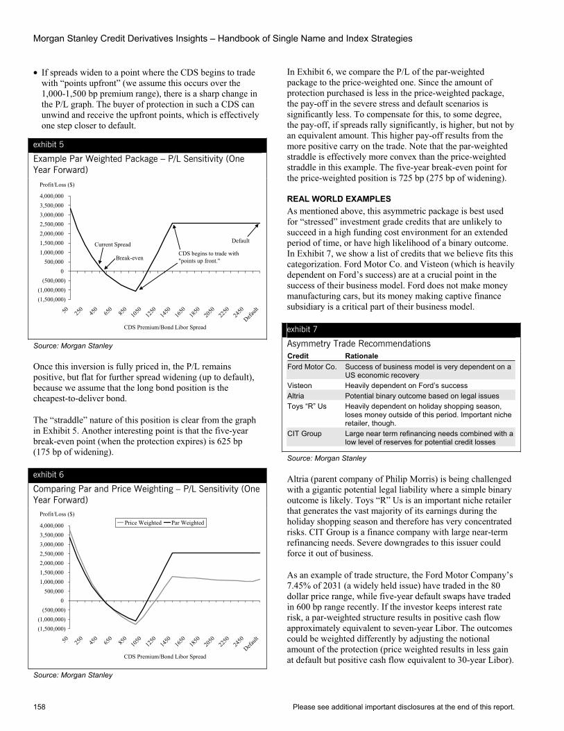
Morgan Stanley Credit Derivatives Insights – Handbook of Single Name and Index Strategies
158 Please see additional important disclosures at the end of this report.
• If spreads widen to a point where the CDS begins to trade with “points upfront” (we assume this occurs over the 1,000-1,500 bp premium range), there is a sharp change in the P/L graph. The buyer of protection in such a CDS can unwind and receive the upfront points, which is effectively one step closer to default.
exhibit 5
Example Par Weighted Package – P/L Sensitivity (One Year Forward)
Profit/Loss ($)
(1,500,000)(1,000,000)
(500,000)0
500,0001,000,0001,500,0002,000,0002,500,0003,000,0003,500,0004,000,000
50 250
450
650
850
1050
1250
1450
1650
1850
2050
2250
2450
Default
CDS Premium/Bond Libor Spread
Current Spread
Break-even
Default
CDS begins to trade with"points up front."
Source: Morgan Stanley
Once this inversion is fully priced in, the P/L remains positive, but flat for further spread widening (up to default), because we assume that the long bond position is the cheapest-to-deliver bond.
The “straddle” nature of this position is clear from the graph in Exhibit 5. Another interesting point is that the five-year break-even point (when the protection expires) is 625 bp (175 bp of widening).
exhibit 6
Comparing Par and Price Weighting – P/L Sensitivity (One Year Forward)
Profit/Loss ($)
(1,500,000)(1,000,000)
(500,000)0
500,0001,000,0001,500,0002,000,0002,500,0003,000,0003,500,0004,000,000
50 250
450
650
850
1050
1250
1450
1650
1850
2050
2250
2450
Default
CDS Premium/Bond Libor Spread
Price Weighted Par Weighted
Source: Morgan Stanley
In Exhibit 6, we compare the P/L of the par-weighted package to the price-weighted one. Since the amount of protection purchased is less in the price-weighted package, the pay-off in the severe stress and default scenarios is significantly less. To compensate for this, to some degree, the pay-off, if spreads rally significantly, is higher, but not by an equivalent amount. This higher pay-off results from the more positive carry on the trade. Note that the par-weighted straddle is effectively more convex than the price-weighted straddle in this example. The five-year break-even point for the price-weighted position is 725 bp (275 bp of widening).
REAL WORLD EXAMPLES As mentioned above, this asymmetric package is best used for “stressed” investment grade credits that are unlikely to succeed in a high funding cost environment for an extended period of time, or have high likelihood of a binary outcome. In Exhibit 7, we show a list of credits that we believe fits this categorization. Ford Motor Co. and Visteon (which is heavily dependent on Ford’s success) are at a crucial point in the success of their business model. Ford does not make money manufacturing cars, but its money making captive finance subsidiary is a critical part of their business model.
exhibit 7
Asymmetry Trade Recommendations Credit Rationale Ford Motor Co. Success of business model is very dependent on a
US economic recovery Visteon Heavily dependent on Ford’s success Altria Potential binary outcome based on legal issues Toys “R” Us Heavily dependent on holiday shopping season,
loses money outside of this period. Important niche retailer, though.
CIT Group Large near term refinancing needs combined with a low level of reserves for potential credit losses
Source: Morgan Stanley
Altria (parent company of Philip Morris) is being challenged with a gigantic potential legal liability where a simple binary outcome is likely. Toys “R” Us is an important niche retailer that generates the vast majority of its earnings during the holiday shopping season and therefore has very concentrated risks. CIT Group is a finance company with large near-term refinancing needs. Severe downgrades to this issuer could force it out of business.
As an example of trade structure, the Ford Motor Company’s 7.45% of 2031 (a widely held issue) have traded in the 80 dollar price range, while five-year default swaps have traded in 600 bp range recently. If the investor keeps interest rate risk, a par-weighted structure results in positive cash flow approximately equivalent to seven-year Libor. The outcomes could be weighted differently by adjusting the notional amount of the protection (price weighted results in less gain at default but positive cash flow equivalent to 30-year Libor).
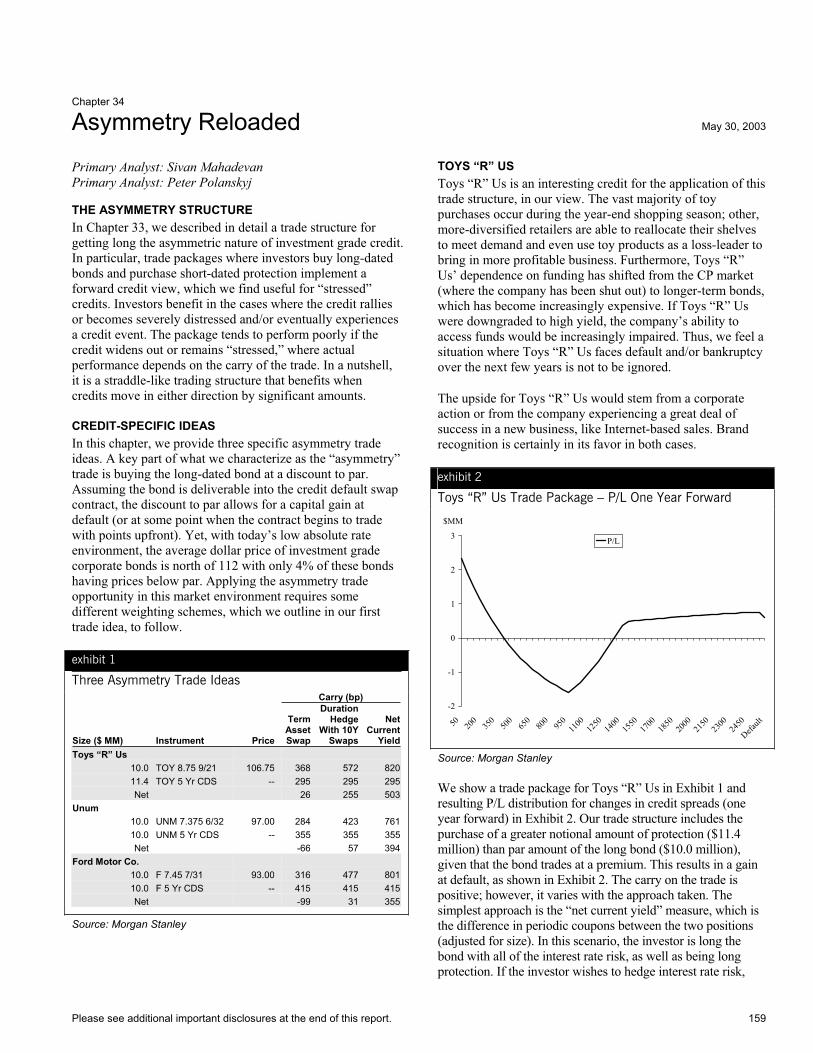
Please see additional important disclosures at the end of this report. 159
Chapter 34
Asymmetry Reloaded May 30, 2003
Primary Analyst: Sivan Mahadevan Primary Analyst: Peter Polanskyj
THE ASYMMETRY STRUCTURE In Chapter 33, we described in detail a trade structure for getting long the asymmetric nature of investment grade credit. In particular, trade packages where investors buy long-dated bonds and purchase short-dated protection implement a forward credit view, which we find useful for “stressed” credits. Investors benefit in the cases where the credit rallies or becomes severely distressed and/or eventually experiences a credit event. The package tends to perform poorly if the credit widens out or remains “stressed,” where actual performance depends on the carry of the trade. In a nutshell, it is a straddle-like trading structure that benefits when credits move in either direction by significant amounts.
CREDIT-SPECIFIC IDEAS In this chapter, we provide three specific asymmetry trade ideas. A key part of what we characterize as the “asymmetry” trade is buying the long-dated bond at a discount to par. Assuming the bond is deliverable into the credit default swap contract, the discount to par allows for a capital gain at default (or at some point when the contract begins to trade with points upfront). Yet, with today’s low absolute rate environment, the average dollar price of investment grade corporate bonds is north of 112 with only 4% of these bonds having prices below par. Applying the asymmetry trade opportunity in this market environment requires some different weighting schemes, which we outline in our first trade idea, to follow.
exhibit 1
Three Asymmetry Trade Ideas Carry (bp)
Size ($ MM) Instrument Price
Term Asset Swap
Duration Hedge
With 10Y Swaps
NetCurrent
YieldToys “R” Us
10.0 TOY 8.75 9/21 106.75 368 572 82011.4 TOY 5 Yr CDS -- 295 295 295Net 26 255 503
Unum 10.0 UNM 7.375 6/32 97.00 284 423 76110.0 UNM 5 Yr CDS -- 355 355 355Net -66 57 394
Ford Motor Co. 10.0 F 7.45 7/31 93.00 316 477 80110.0 F 5 Yr CDS -- 415 415 415Net -99 31 355
Source: Morgan Stanley
TOYS “R” US Toys “R” Us is an interesting credit for the application of this trade structure, in our view. The vast majority of toy purchases occur during the year-end shopping season; other, more-diversified retailers are able to reallocate their shelves to meet demand and even use toy products as a loss-leader to bring in more profitable business. Furthermore, Toys “R” Us’ dependence on funding has shifted from the CP market (where the company has been shut out) to longer-term bonds, which has become increasingly expensive. If Toys “R” Us were downgraded to high yield, the company’s ability to access funds would be increasingly impaired. Thus, we feel a situation where Toys “R” Us faces default and/or bankruptcy over the next few years is not to be ignored.
The upside for Toys “R” Us would stem from a corporate action or from the company experiencing a great deal of success in a new business, like Internet-based sales. Brand recognition is certainly in its favor in both cases.
exhibit 2
Toys “R” Us Trade Package – P/L One Year Forward
$MM
-2
-1
0
1
2
3
50 200
350
500
650
800
950
1100
1250
1400
1550
1700
1850
2000
2150
2300
2450
Default
P/L
Source: Morgan Stanley
We show a trade package for Toys “R” Us in Exhibit 1 and resulting P/L distribution for changes in credit spreads (one year forward) in Exhibit 2. Our trade structure includes the purchase of a greater notional amount of protection ($11.4 million) than par amount of the long bond ($10.0 million), given that the bond trades at a premium. This results in a gain at default, as shown in Exhibit 2. The carry on the trade is positive; however, it varies with the approach taken. The simplest approach is the “net current yield” measure, which is the difference in periodic coupons between the two positions (adjusted for size). In this scenario, the investor is long the bond with all of the interest rate risk, as well as being long protection. If the investor wishes to hedge interest rate risk,
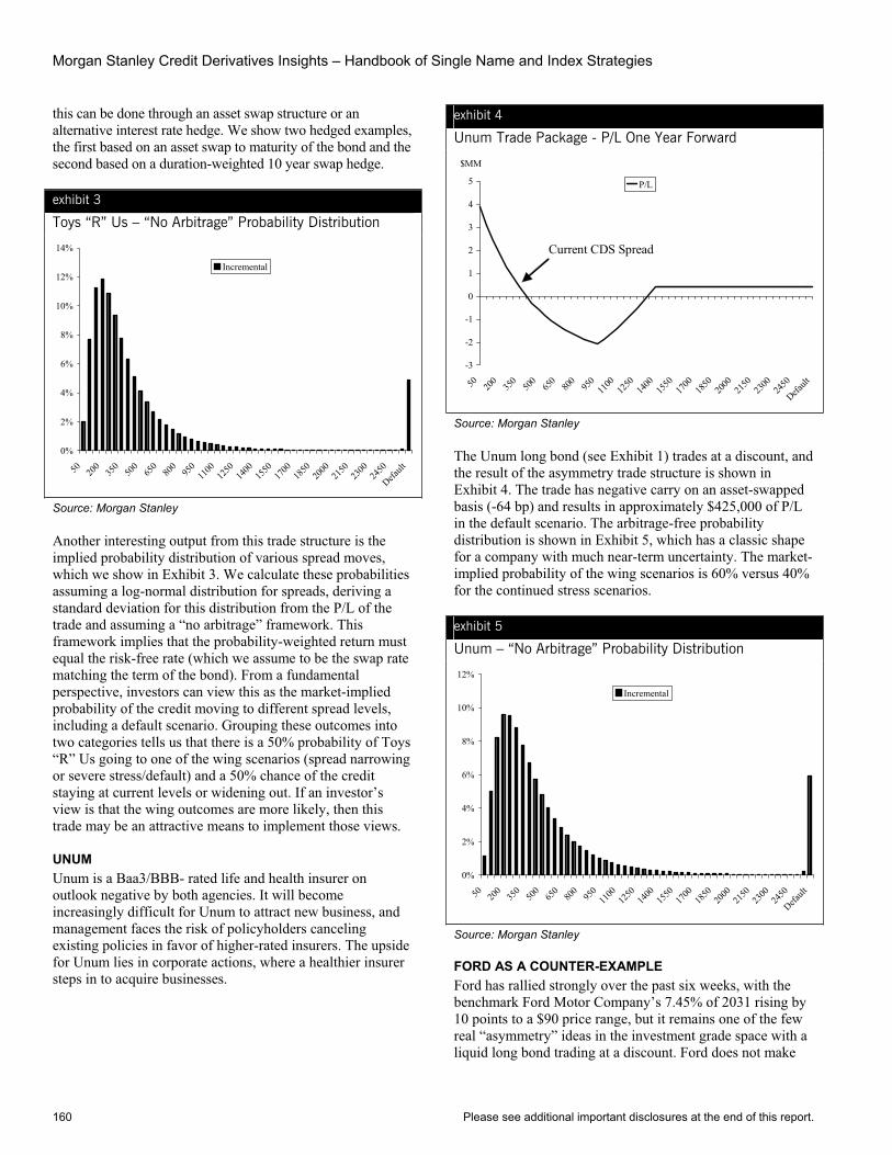
Morgan Stanley Credit Derivatives Insights – Handbook of Single Name and Index Strategies
160 Please see additional important disclosures at the end of this report.
this can be done through an asset swap structure or an alternative interest rate hedge. We show two hedged examples, the first based on an asset swap to maturity of the bond and the second based on a duration-weighted 10 year swap hedge.
exhibit 3
Toys “R” Us – “No Arbitrage” Probability Distribution
0%
2%
4%
6%
8%
10%
12%
14%
50 200
350
500
650
800
950
1100
1250
1400
1550
1700
1850
2000
2150
2300
2450
Default
Incremental
Source: Morgan Stanley
Another interesting output from this trade structure is the implied probability distribution of various spread moves, which we show in Exhibit 3. We calculate these probabilities assuming a log-normal distribution for spreads, deriving a standard deviation for this distribution from the P/L of the trade and assuming a “no arbitrage” framework. This framework implies that the probability-weighted return must equal the risk-free rate (which we assume to be the swap rate matching the term of the bond). From a fundamental perspective, investors can view this as the market-implied probability of the credit moving to different spread levels, including a default scenario. Grouping these outcomes into two categories tells us that there is a 50% probability of Toys “R” Us going to one of the wing scenarios (spread narrowing or severe stress/default) and a 50% chance of the credit staying at current levels or widening out. If an investor’s view is that the wing outcomes are more likely, then this trade may be an attractive means to implement those views.
UNUMUnum is a Baa3/BBB- rated life and health insurer on outlook negative by both agencies. It will become increasingly difficult for Unum to attract new business, and management faces the risk of policyholders canceling existing policies in favor of higher-rated insurers. The upside for Unum lies in corporate actions, where a healthier insurer steps in to acquire businesses.
exhibit 4
Unum Trade Package - P/L One Year Forward
$MM
-3
-2
-1
0
1
2
3
4
5
50 200
350
500
650
800
950
1100
1250
1400
1550
1700
1850
2000
2150
2300
2450
Default
P/L
Current CDS Spread
Source: Morgan Stanley
The Unum long bond (see Exhibit 1) trades at a discount, and the result of the asymmetry trade structure is shown in Exhibit 4. The trade has negative carry on an asset-swapped basis (-64 bp) and results in approximately $425,000 of P/L in the default scenario. The arbitrage-free probability distribution is shown in Exhibit 5, which has a classic shape for a company with much near-term uncertainty. The market-implied probability of the wing scenarios is 60% versus 40% for the continued stress scenarios.
exhibit 5
Unum – “No Arbitrage” Probability Distribution
0%
2%
4%
6%
8%
10%
12%
50 200
350
500
650
800
950
1100
1250
1400
1550
1700
1850
2000
2150
2300
2450
Default
Incremental
Source: Morgan Stanley
FORD AS A COUNTER-EXAMPLE Ford has rallied strongly over the past six weeks, with the benchmark Ford Motor Company’s 7.45% of 2031 rising by 10 points to a $90 price range, but it remains one of the few real “asymmetry” ideas in the investment grade space with a liquid long bond trading at a discount. Ford does not make
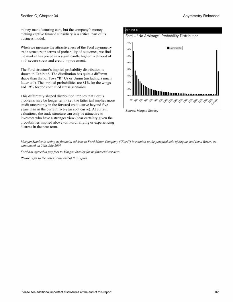
Section C, Chapter 34 Asymmetry Reloaded
Please see additional important disclosures at the end of this report. 161
money manufacturing cars, but the company’s money-making captive finance subsidiary is a critical part of its business model.
When we measure the attractiveness of the Ford asymmetry trade structure in terms of probability of outcomes, we find the market has priced in a significantly higher likelihood of both severe stress and credit improvement.
The Ford structure’s implied probability distribution is shown in Exhibit 6. The distribution has quite a different shape than that of Toys “R” Us or Unum (including a much fatter tail). The implied probabilities are 81% for the wings and 19% for the continued stress scenarios.
This differently shaped distribution implies that Ford’s problems may be longer term (i.e., the fatter tail implies more credit uncertainty in the forward credit curve beyond five years than in the current five-year spot curve). At current valuations, the trade structure can only be attractive to investors who have a stronger view (near certainty given the probabilities implied above) on Ford rallying or experiencing distress in the near term.
exhibit 6
Ford – “No Arbitrage” Probability Distribution
0%
2%
4%
6%
8%
10%
12%
14%
16%
50 200
350
500
650
800
950
1100
1250
1400
1550
1700
1850
2000
2150
2300
2450
Default
Incremental
Source: Morgan Stanley
Morgan Stanley is acting as financial advisor to Ford Motor Company ("Ford") in relation to the potential sale of Jaguar and Land Rover, as announced on 26th July 2007
Ford has agreed to pay fees to Morgan Stanley for its financial services.
Please refer to the notes at the end of this report.
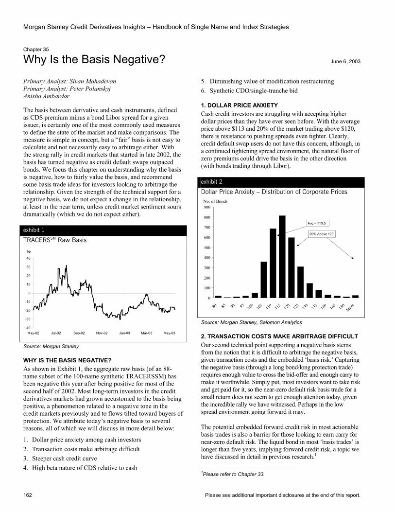
Morgan Stanley Credit Derivatives Insights – Handbook of Single Name and Index Strategies
162 Please see additional important disclosures at the end of this report.
Chapter 35
Why Is the Basis Negative? June 6, 2003
Primary Analyst: Sivan Mahadevan Primary Analyst: Peter Polanskyj Anisha Ambardar
The basis between derivative and cash instruments, defined as CDS premium minus a bond Libor spread for a given issuer, is certainly one of the most commonly used measures to define the state of the market and make comparisons. The measure is simple in concept, but a “fair” basis is not easy to calculate and not necessarily easy to arbitrage either. With the strong rally in credit markets that started in late 2002, the basis has turned negative as credit default swaps outpaced bonds. We focus this chapter on understanding why the basis is negative, how to fairly value the basis, and recommend some basis trade ideas for investors looking to arbitrage the relationship. Given the strength of the technical support for a negative basis, we do not expect a change in the relationship, at least in the near term, unless credit market sentiment sours dramatically (which we do not expect either).
exhibit 1
TRACERSSM Raw Basis
bp
-40
-30
-20
-10
0
10
20
30
40
May-02 Jul-02 Sep-02 Nov-02 Jan-03 Mar-03 May-03
Source: Morgan Stanley
WHY IS THE BASIS NEGATIVE? As shown in Exhibit 1, the aggregate raw basis (of an 88-name subset of the 100-name synthetic TRACERSSM) has been negative this year after being positive for most of the second half of 2002. Most long-term investors in the credit derivatives markets had grown accustomed to the basis being positive, a phenomenon related to a negative tone in the credit markets previously and to flows tilted toward buyers of protection. We attribute today’s negative basis to several reasons, all of which we will discuss in more detail below:
1. Dollar price anxiety among cash investors 2. Transaction costs make arbitrage difficult 3. Steeper cash credit curve 4. High beta nature of CDS relative to cash
5. Diminishing value of modification restructuring 6. Synthetic CDO/single-tranche bid
1. DOLLAR PRICE ANXIETY Cash credit investors are struggling with accepting higher dollar prices than they have ever seen before. With the average price above $113 and 20% of the market trading above $120, there is resistance to pushing spreads even tighter. Clearly, credit default swap users do not have this concern, although, in a continued tightening spread environment, the natural floor of zero premiums could drive the basis in the other direction (with bonds trading through Libor).
exhibit 2
Dollar Price Anxiety – Distribution of Corporate Prices No. of Bonds
0
100
200
300
400
500
600
700
800
900
80 85 90 95 100
105
110
115
120
125
130
135
140
145
150
More
Avg = 113.5
20% Above 120
Source: Morgan Stanley, Salomon Analytics
2. TRANSACTION COSTS MAKE ARBITRAGE DIFFICULT Our second technical point supporting a negative basis stems from the notion that it is difficult to arbitrage the negative basis, given transaction costs and the embedded ‘basis risk.’ Capturing the negative basis (through a long bond/long protection trade) requires enough value to cross the bid-offer and enough carry to make it worthwhile. Simply put, most investors want to take risk and get paid for it, so the near-zero default risk basis trade for a small return does not seem to get enough attention today, given the incredible rally we have witnessed. Perhaps in the low spread environment going forward it may.
The potential embedded forward credit risk in most actionable basis trades is also a barrier for those looking to earn carry for near-zero default risk. The liquid bond in most ‘basis trades’ is longer than five years, implying forward credit risk, a topic we have discussed in detail in previous research.1
1Please refer to Chapter 33.
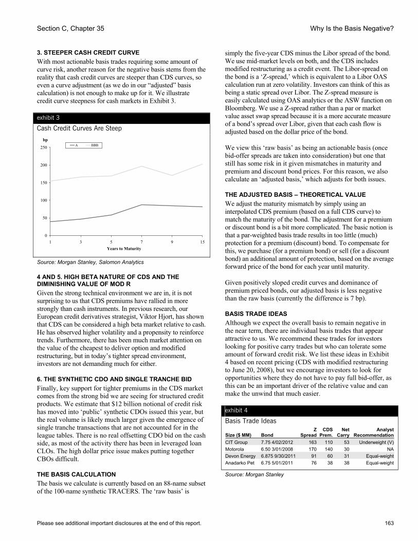
Section C, Chapter 35 Why Is the Basis Negative?
Please see additional important disclosures at the end of this report. 163
3. STEEPER CASH CREDIT CURVE With most actionable basis trades requiring some amount of curve risk, another reason for the negative basis stems from the reality that cash credit curves are steeper than CDS curves, so even a curve adjustment (as we do in our “adjusted” basis calculation) is not enough to make up for it. We illustrate credit curve steepness for cash markets in Exhibit 3.
exhibit 3
Cash Credit Curves Are Steep
0
50
100
150
200
250
1 3 5 7 9 15
A BBBbp
Years to Maturity
Source: Morgan Stanley, Salomon Analytics
4 AND 5. HIGH BETA NATURE OF CDS AND THE DIMINISHING VALUE OF MOD R Given the strong technical environment we are in, it is not surprising to us that CDS premiums have rallied in more strongly than cash instruments. In previous research, our European credit derivatives strategist, Viktor Hjort, has shown that CDS can be considered a high beta market relative to cash. He has observed higher volatility and a propensity to reinforce trends. Furthermore, there has been much market attention on the value of the cheapest to deliver option and modified restructuring, but in today’s tighter spread environment, investors are not demanding much for either.
6. THE SYNTHETIC CDO AND SINGLE TRANCHE BID Finally, key support for tighter premiums in the CDS market comes from the strong bid we are seeing for structured credit products. We estimate that $12 billion notional of credit risk has moved into ‘public’ synthetic CDOs issued this year, but the real volume is likely much larger given the emergence of single tranche transactions that are not accounted for in the league tables. There is no real offsetting CDO bid on the cash side, as most of the activity there has been in leveraged loan CLOs. The high dollar price issue makes putting together CBOs difficult.
THE BASIS CALCULATION The basis we calculate is currently based on an 88-name subset of the 100-name synthetic TRACERS. The ‘raw basis’ is
simply the five-year CDS minus the Libor spread of the bond. We use mid-market levels on both, and the CDS includes modified restructuring as a credit event. The Libor-spread on the bond is a ‘Z-spread,’ which is equivalent to a Libor OAS calculation run at zero volatility. Investors can think of this as being a static spread over Libor. The Z-spread measure is easily calculated using OAS analytics or the ASW function on Bloomberg. We use a Z-spread rather than a par or market value asset swap spread because it is a more accurate measure of a bond’s spread over Libor, given that each cash flow is adjusted based on the dollar price of the bond.
We view this ‘raw basis’ as being an actionable basis (once bid-offer spreads are taken into consideration) but one that still has some risk in it given mismatches in maturity and premium and discount bond prices. For this reason, we also calculate an ‘adjusted basis,’ which adjusts for both issues.
THE ADJUSTED BASIS – THEORETICAL VALUE We adjust the maturity mismatch by simply using an interpolated CDS premium (based on a full CDS curve) to match the maturity of the bond. The adjustment for a premium or discount bond is a bit more complicated. The basic notion is that a par-weighted basis trade results in too little (much) protection for a premium (discount) bond. To compensate for this, we purchase (for a premium bond) or sell (for a discount bond) an additional amount of protection, based on the average forward price of the bond for each year until maturity.
Given positively sloped credit curves and dominance of premium priced bonds, our adjusted basis is less negative than the raw basis (currently the difference is 7 bp).
BASIS TRADE IDEAS Although we expect the overall basis to remain negative in the near term, there are individual basis trades that appear attractive to us. We recommend these trades for investors looking for positive carry trades but who can tolerate some amount of forward credit risk. We list these ideas in Exhibit 4 based on recent pricing (CDS with modified restructuring to June 20, 2008), but we encourage investors to look for opportunities where they do not have to pay full bid-offer, as this can be an important driver of the relative value and can make the unwind that much easier.
exhibit 4
Basis Trade Ideas
Size ($ MM) Bond Z
SpreadCDS
Prem. Net
CarryAnalyst
RecommendationCIT Group 7.75 4/02/2012 163 110 53 Underweight (V)Motorola 6.50 3/01/2008 170 140 30 NADevon Energy 6.875 9/30/2011 91 60 31 Equal-weightAnadarko Pet 6.75 5/01/2011 76 38 38 Equal-weight
Source: Morgan Stanley
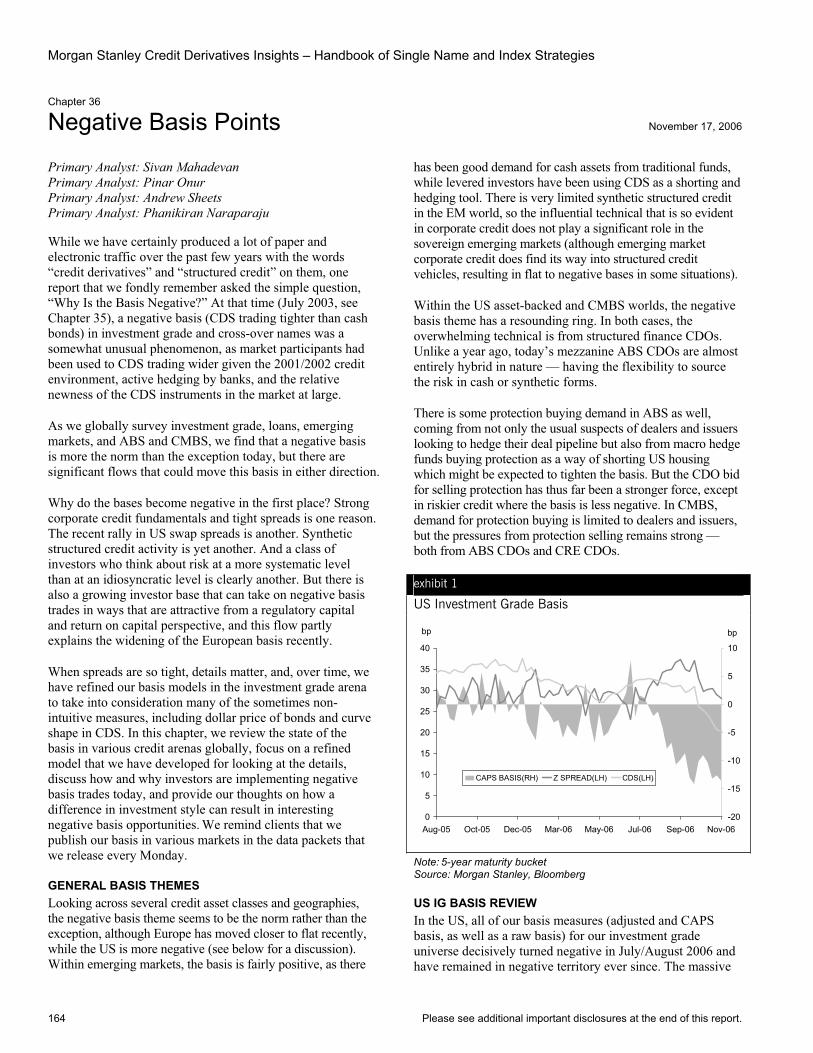
Morgan Stanley Credit Derivatives Insights – Handbook of Single Name and Index Strategies
164 Please see additional important disclosures at the end of this report.
Chapter 36
Negative Basis Points November 17, 2006
Primary Analyst: Sivan Mahadevan Primary Analyst: Pinar Onur Primary Analyst: Andrew Sheets Primary Analyst: Phanikiran Naraparaju
While we have certainly produced a lot of paper and electronic traffic over the past few years with the words “credit derivatives” and “structured credit” on them, one report that we fondly remember asked the simple question, “Why Is the Basis Negative?” At that time (July 2003, see Chapter 35), a negative basis (CDS trading tighter than cash bonds) in investment grade and cross-over names was a somewhat unusual phenomenon, as market participants had been used to CDS trading wider given the 2001/2002 credit environment, active hedging by banks, and the relative newness of the CDS instruments in the market at large.
As we globally survey investment grade, loans, emerging markets, and ABS and CMBS, we find that a negative basis is more the norm than the exception today, but there are significant flows that could move this basis in either direction.
Why do the bases become negative in the first place? Strong corporate credit fundamentals and tight spreads is one reason. The recent rally in US swap spreads is another. Synthetic structured credit activity is yet another. And a class of investors who think about risk at a more systematic level than at an idiosyncratic level is clearly another. But there is also a growing investor base that can take on negative basis trades in ways that are attractive from a regulatory capital and return on capital perspective, and this flow partly explains the widening of the European basis recently.
When spreads are so tight, details matter, and, over time, we have refined our basis models in the investment grade arena to take into consideration many of the sometimes non-intuitive measures, including dollar price of bonds and curve shape in CDS. In this chapter, we review the state of the basis in various credit arenas globally, focus on a refined model that we have developed for looking at the details, discuss how and why investors are implementing negative basis trades today, and provide our thoughts on how a difference in investment style can result in interesting negative basis opportunities. We remind clients that we publish our basis in various markets in the data packets that we release every Monday.
GENERAL BASIS THEMES Looking across several credit asset classes and geographies, the negative basis theme seems to be the norm rather than the exception, although Europe has moved closer to flat recently, while the US is more negative (see below for a discussion). Within emerging markets, the basis is fairly positive, as there
has been good demand for cash assets from traditional funds, while levered investors have been using CDS as a shorting and hedging tool. There is very limited synthetic structured credit in the EM world, so the influential technical that is so evident in corporate credit does not play a significant role in the sovereign emerging markets (although emerging market corporate credit does find its way into structured credit vehicles, resulting in flat to negative bases in some situations).
Within the US asset-backed and CMBS worlds, the negative basis theme has a resounding ring. In both cases, the overwhelming technical is from structured finance CDOs. Unlike a year ago, today’s mezzanine ABS CDOs are almost entirely hybrid in nature — having the flexibility to source the risk in cash or synthetic forms.
There is some protection buying demand in ABS as well, coming from not only the usual suspects of dealers and issuers looking to hedge their deal pipeline but also from macro hedge funds buying protection as a way of shorting US housing which might be expected to tighten the basis. But the CDO bid for selling protection has thus far been a stronger force, except in riskier credit where the basis is less negative. In CMBS, demand for protection buying is limited to dealers and issuers, but the pressures from protection selling remains strong — both from ABS CDOs and CRE CDOs.
exhibit 1
US Investment Grade Basis
bp
0
5
10
15
20
25
30
35
40
Aug-05 Oct-05 Dec-05 Mar-06 May-06 Jul-06 Sep-06 Nov-06-20
-15
-10
-5
0
5
10
CAPS BASIS(RH) Z SPREAD(LH) CDS(LH)
bp
Note: 5-year maturity bucket Source: Morgan Stanley, Bloomberg
US IG BASIS REVIEW In the US, all of our basis measures (adjusted and CAPS basis, as well as a raw basis) for our investment grade universe decisively turned negative in July/August 2006 and have remained in negative territory ever since. The massive
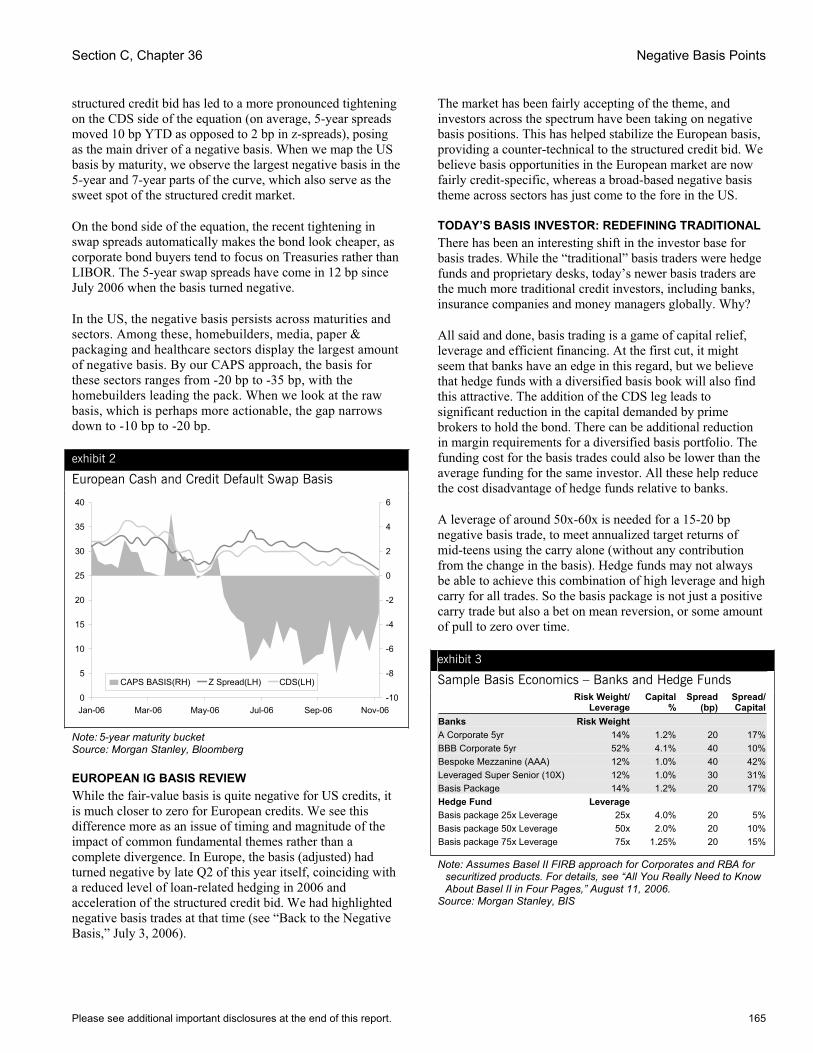
Section C, Chapter 36 Negative Basis Points
Please see additional important disclosures at the end of this report. 165
structured credit bid has led to a more pronounced tightening on the CDS side of the equation (on average, 5-year spreads moved 10 bp YTD as opposed to 2 bp in z-spreads), posing as the main driver of a negative basis. When we map the US basis by maturity, we observe the largest negative basis in the 5-year and 7-year parts of the curve, which also serve as the sweet spot of the structured credit market.
On the bond side of the equation, the recent tightening in swap spreads automatically makes the bond look cheaper, as corporate bond buyers tend to focus on Treasuries rather than LIBOR. The 5-year swap spreads have come in 12 bp since July 2006 when the basis turned negative.
In the US, the negative basis persists across maturities and sectors. Among these, homebuilders, media, paper & packaging and healthcare sectors display the largest amount of negative basis. By our CAPS approach, the basis for these sectors ranges from -20 bp to -35 bp, with the homebuilders leading the pack. When we look at the raw basis, which is perhaps more actionable, the gap narrows down to -10 bp to -20 bp.
exhibit 2
European Cash and Credit Default Swap Basis
0
5
10
15
20
25
30
35
40
Jan-06 Mar-06 May-06 Jul-06 Sep-06 Nov-06-10
-8
-6
-4
-2
0
2
4
6
CAPS BASIS(RH) Z Spread(LH) CDS(LH)
Note: 5-year maturity bucket Source: Morgan Stanley, Bloomberg
EUROPEAN IG BASIS REVIEW While the fair-value basis is quite negative for US credits, it is much closer to zero for European credits. We see this difference more as an issue of timing and magnitude of the impact of common fundamental themes rather than a complete divergence. In Europe, the basis (adjusted) had turned negative by late Q2 of this year itself, coinciding with a reduced level of loan-related hedging in 2006 and acceleration of the structured credit bid. We had highlighted negative basis trades at that time (see “Back to the Negative Basis,” July 3, 2006).
The market has been fairly accepting of the theme, and investors across the spectrum have been taking on negative basis positions. This has helped stabilize the European basis, providing a counter-technical to the structured credit bid. We believe basis opportunities in the European market are now fairly credit-specific, whereas a broad-based negative basis theme across sectors has just come to the fore in the US.
TODAY’S BASIS INVESTOR: REDEFINING TRADITIONAL There has been an interesting shift in the investor base for basis trades. While the “traditional” basis traders were hedge funds and proprietary desks, today’s newer basis traders are the much more traditional credit investors, including banks, insurance companies and money managers globally. Why?
All said and done, basis trading is a game of capital relief, leverage and efficient financing. At the first cut, it might seem that banks have an edge in this regard, but we believe that hedge funds with a diversified basis book will also find this attractive. The addition of the CDS leg leads to significant reduction in the capital demanded by prime brokers to hold the bond. There can be additional reduction in margin requirements for a diversified basis portfolio. The funding cost for the basis trades could also be lower than the average funding for the same investor. All these help reduce the cost disadvantage of hedge funds relative to banks.
A leverage of around 50x-60x is needed for a 15-20 bp negative basis trade, to meet annualized target returns of mid-teens using the carry alone (without any contribution from the change in the basis). Hedge funds may not always be able to achieve this combination of high leverage and high carry for all trades. So the basis package is not just a positive carry trade but also a bet on mean reversion, or some amount of pull to zero over time.
exhibit 3
Sample Basis Economics – Banks and Hedge Funds Risk Weight/
Leverage Capital
%Spread
(bp)Spread/Capital
Banks Risk Weight A Corporate 5yr 14% 1.2% 20 17%BBB Corporate 5yr 52% 4.1% 40 10%Bespoke Mezzanine (AAA) 12% 1.0% 40 42%Leveraged Super Senior (10X) 12% 1.0% 30 31%Basis Package 14% 1.2% 20 17%Hedge Fund Leverage Basis package 25x Leverage 25x 4.0% 20 5%Basis package 50x Leverage 50x 2.0% 20 10%Basis package 75x Leverage 75x 1.25% 20 15%
Note: Assumes Basel II FIRB approach for Corporates and RBA for securitized products. For details, see “All You Really Need to Know About Basel II in Four Pages,” August 11, 2006.
Source: Morgan Stanley, BIS
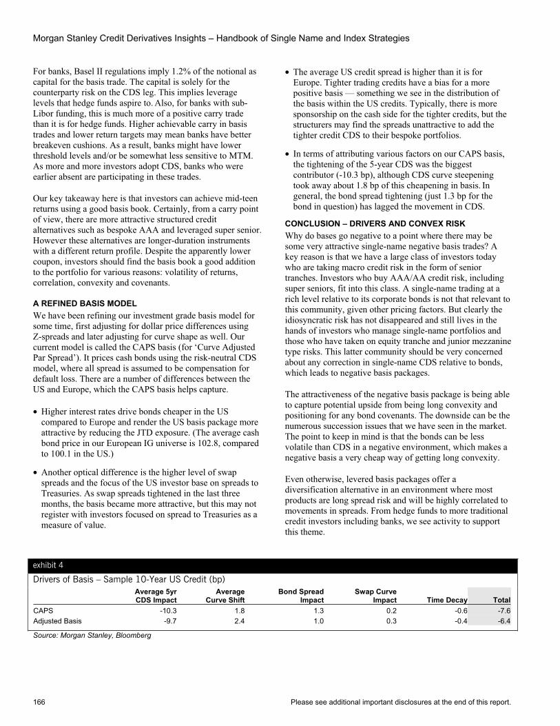
Morgan Stanley Credit Derivatives Insights – Handbook of Single Name and Index Strategies
166 Please see additional important disclosures at the end of this report.
For banks, Basel II regulations imply 1.2% of the notional as capital for the basis trade. The capital is solely for the counterparty risk on the CDS leg. This implies leverage levels that hedge funds aspire to. Also, for banks with sub-Libor funding, this is much more of a positive carry trade than it is for hedge funds. Higher achievable carry in basis trades and lower return targets may mean banks have better breakeven cushions. As a result, banks might have lower threshold levels and/or be somewhat less sensitive to MTM. As more and more investors adopt CDS, banks who were earlier absent are participating in these trades.
Our key takeaway here is that investors can achieve mid-teen returns using a good basis book. Certainly, from a carry point of view, there are more attractive structured credit alternatives such as bespoke AAA and leveraged super senior. However these alternatives are longer-duration instruments with a different return profile. Despite the apparently lower coupon, investors should find the basis book a good addition to the portfolio for various reasons: volatility of returns, correlation, convexity and covenants.
A REFINED BASIS MODEL We have been refining our investment grade basis model for some time, first adjusting for dollar price differences using Z-spreads and later adjusting for curve shape as well. Our current model is called the CAPS basis (for ‘Curve Adjusted Par Spread’). It prices cash bonds using the risk-neutral CDS model, where all spread is assumed to be compensation for default loss. There are a number of differences between the US and Europe, which the CAPS basis helps capture.
• Higher interest rates drive bonds cheaper in the US compared to Europe and render the US basis package more attractive by reducing the JTD exposure. (The average cash bond price in our European IG universe is 102.8, compared to 100.1 in the US.)
• Another optical difference is the higher level of swap spreads and the focus of the US investor base on spreads to Treasuries. As swap spreads tightened in the last three months, the basis became more attractive, but this may not register with investors focused on spread to Treasuries as a measure of value.
• The average US credit spread is higher than it is for Europe. Tighter trading credits have a bias for a more positive basis — something we see in the distribution of the basis within the US credits. Typically, there is more sponsorship on the cash side for the tighter credits, but the structurers may find the spreads unattractive to add the tighter credit CDS to their bespoke portfolios.
• In terms of attributing various factors on our CAPS basis, the tightening of the 5-year CDS was the biggest contributor (-10.3 bp), although CDS curve steepening took away about 1.8 bp of this cheapening in basis. In general, the bond spread tightening (just 1.3 bp for the bond in question) has lagged the movement in CDS.
CONCLUSION – DRIVERS AND CONVEX RISK Why do bases go negative to a point where there may be some very attractive single-name negative basis trades? A key reason is that we have a large class of investors today who are taking macro credit risk in the form of senior tranches. Investors who buy AAA/AA credit risk, including super seniors, fit into this class. A single-name trading at a rich level relative to its corporate bonds is not that relevant to this community, given other pricing factors. But clearly the idiosyncratic risk has not disappeared and still lives in the hands of investors who manage single-name portfolios and those who have taken on equity tranche and junior mezzanine type risks. This latter community should be very concerned about any correction in single-name CDS relative to bonds, which leads to negative basis packages.
The attractiveness of the negative basis package is being able to capture potential upside from being long convexity and positioning for any bond covenants. The downside can be the numerous succession issues that we have seen in the market. The point to keep in mind is that the bonds can be less volatile than CDS in a negative environment, which makes a negative basis a very cheap way of getting long convexity.
Even otherwise, levered basis packages offer a diversification alternative in an environment where most products are long spread risk and will be highly correlated to movements in spreads. From hedge funds to more traditional credit investors including banks, we see activity to support this theme.
exhibit 4
Drivers of Basis – Sample 10-Year US Credit (bp) Average 5yr CDS Impact
Average Curve Shift
Bond Spread Impact
Swap Curve Impact Time Decay Total
CAPS -10.3 1.8 1.3 0.2 -0.6 -7.6Adjusted Basis -9.7 2.4 1.0 0.3 -0.4 -6.4
Source: Morgan Stanley, Bloomberg
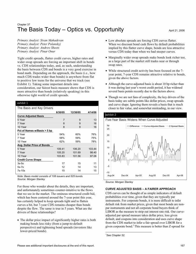
Please see additional important disclosures at the end of this report. 167
Chapter 37
The Basis Today – Optics vs. Opportunity April 21, 2006
Primary Analyst: Sivan Mahadevan Primary Analyst: Peter Polanskyj Primary Analyst: Andrew Sheets Primary Analyst: Pinar Onur
Tight credit spreads, flatter credit curves, higher rates and wider swap spreads are forcing an important shift in bonds vs. CDS relationships today, and, as such, understanding the basis between CDS and bonds is a very good exercise in bond math. Depending on the approach, the basis (i.e., how much CDS trades wider than bonds) is anywhere from flat to positive low teens for the universe that we track (see Exhibit 1). Taking some important details into consideration, our fairest basis measure shows that CDS is more attractive than bonds (relatively speaking) in this otherwise tight world of credit spreads.
exhibit 1
The Basis and Key Drivers 6/30/05 12/30/05 4/14/06Curve Adjusted Basis 5 Year 7 9 137 Year 8 9 1610 Year 8 9 16Pct of Names w/Basis > 5 bp 5 Year 54% 60% 76%7 Year 58% 59% 75%10 Year 62% 59% 78%Avg. Dollar Price of Bonds 5 Year 109.41 106.20 103.447 Year 105.20 101.69 98.4010 Year 103.83 101.56 97.06Credit Curve Shape 3s-5s 17 15 115s-7s 12 14 137s-10s 15 14 15
Note: Basis model consists of 108 issuers and 525 bonds. Source: Morgan Stanley
For those who wonder about the details, they are important, and unfortunately sometimes counter-intuitive to the flows that we see in the market. The ominous structured credit bid, which has been centered around the 7-year point this year, has certainly helped to keep spreads tight and to flatten curves a bit, but 7-year CDS remains cheaper than bonds despite the flow. The same is true in 5 years. What are the drivers of these relationships?
• The dollar price impact of significantly higher rates is both making bonds less risky (from a jump-to-default perspective) and tightening bond spreads (investors like lower-priced bonds).
• Low absolute spreads are forcing CDS curves flatter. When we discount bond cash flows by default probabilities implied by this flatter curve shape, bonds are less attractive versus CDS today than when we had steeper curves.
• Marginally wider swap spreads make bonds look richer too, as a large part of the market still trades near or through swap rates.
• While structured credit activity has been focused on the 7-year point, 7-year CDS remains attractive relative to bonds, given the above factors.
• Although the curve-adjusted basis is about 10 bp richer than it was during last year’s worst credit period, it has widened several basis points recently due to the factors above.
• Though we are not fans of complexity, the key drivers of the basis today are subtle points like dollar prices, swap spreads and curve shape. Ignoring them reveals a basis that is much closer to fair value, and somewhat misleading, in our view.
exhibit 2
Five-Year Basis Widens When Curve-Adjusted
bp
-10
-5
0
5
10
15
20
25
Aug-04 Dec-04 Apr-05 Aug-05 Dec-05 Apr-06
Difference Curve-Adjusted Basis Z-Spread Basis
Source: Morgan Stanley
CURVE ADJUSTED BASIS – A FAIRER APPROACH CDS curves can be thought of as simple indicators of default probabilities over time, given that they are typically par instruments. For corporate bonds, it is more difficult to infer default risk from market prices, given that most bonds are non-par instruments and not all corporate bond buyers think of LIBOR as the measure to strip out interest rate risk. Our curve-adjusted par spread measure takes dollar price, loss given default, and coupons into consideration and uses curve shape from the CDS market to infer a fair spread over LIBOR for a given corporate bond.1 This measure is better than Z-spread for
1See Chapter 52.

Morgan Stanley Credit Derivatives Insights – Handbook of Single Name and Index Strategies
168 Please see additional important disclosures at the end of this report.
two reasons. First, it assumes that default risk varies over time (CDS curves). Second, it assumes that losses from default are a function of dollar price and a recovery assumption (Z-spread effectively assumes zero recovery).
When CDS curves steepen, this approach will make bonds look cheaper than on a Z-spread scale, since early coupon payments are deemed less risky. This was a key theme in the market in mid-2004, resulting in a smaller (less positive) basis and thus a more attractive view of bonds versus CDS. Today, with a short-end credit curve flattening, the opposite is true as we see our curve-adjusted basis widening.
We should note that while a simple Z-spread basis has issues, it does reflect a practical way to implement a basis trade. Although our curve-adjusted basis approach shows some additional value in CDS versus cash, it is not an argument for putting on a basis trade, as it is hard to capture the value that we describe using market standard instruments. Rather, it is a guide that today demonstrates that one is paid better for default risk in CDS than bonds in aggregate for our universe of issuers.
THE BOND SIDE OF THE EQUATION As we alluded to, corporate bonds are much more complicated instruments than par CDS instruments. We will make a few obvious but important points. The hybrid (interest rate and credit risk) nature of corporate bonds makes any significant interest rate move relevant to the credit risk of the instrument. Lower dollar prices reduce losses given default (all else being equal), but smaller relative coupons (given higher rates) may more than make up for the reduced risk. However, the general sentiment in the market is that buying bonds with lower dollar prices reduces losses on jump-to-defaults, even if that jump-to-default risk is so remote (based on CDS pricing) that it makes the bond look rich. In today’s environment, both statements are true in that the bonds are looking richer, but investors push them even tighter because they are attracted by lower dollar prices. The other important factor to keep in mind is that in today’s environment, corporate bond buyers have been ignoring LIBOR and focusing on Treasuries, so any swap spread widening makes bonds look automatically richer when compared to CDS. We see many opportunities in corporate bonds, given large relative differences in dollar prices, and address them in a companion report (see the April 21, 2006, Credit Basis Report, “Shooting Below Par”).
THE CDS SIDE OF THE EQUATION While it is hard to argue for one side offering better value than the other in such a tight spread world, one of our key points in this chapter is to go beyond the optics to the opportunities. If current trends continue, CDS is poised to be less risky than bonds (given our basis model). Furthermore, the structured credit machine will stay warm and possibly heat up even more as spring holidays diminish, FAS 155 related trades gain momentum, and the ominous Basel II impact looms even larger.
A key detail on the CDS side is flatter credit curves, although this is really a short-end phenomenon (see Exhibits 1 and 3). In a tighter spread environment, a flatter short-end CDS curve makes near-term default risk marginally higher for bonds (when benchmarked against CDS), so bonds need to price wider to compensate. When this does not happen, bonds appear richer, which is what our basis model is saying.
exhibit 3
The Short-End Is Flatter (YTD)
Spread (bp)
10
15
20
25
30
35
40
45
50
55
3yr 5yr 7yrMaturity
12/31/2005 4/14/2006
Note: Aggregate CDS premiums of 108 issuers in our basis model. Source: Morgan Stanley
exhibit 4
Seven-Year Basis Still Wide Despite Structured Credit Bid
bp
-5
0
5
10
15
20
25
Aug-04 Dec-04 Apr-05 Aug-05 Dec-05 Apr-06
Difference Curve-Adjusted Basis Z-Spread Basis
Source: Morgan Stanley
CONCLUSIONWith the spring holidays behind us, we expect the structured credit bid to pick up in magnitude as the secular themes we have been harping on for the past six months have not changed. That flow, combined with what our relative value tools are telling us, points to the attractiveness of CDS versus bonds in many cases, despite the misleading optics of simply subtracting bond spreads from CDS premiums.
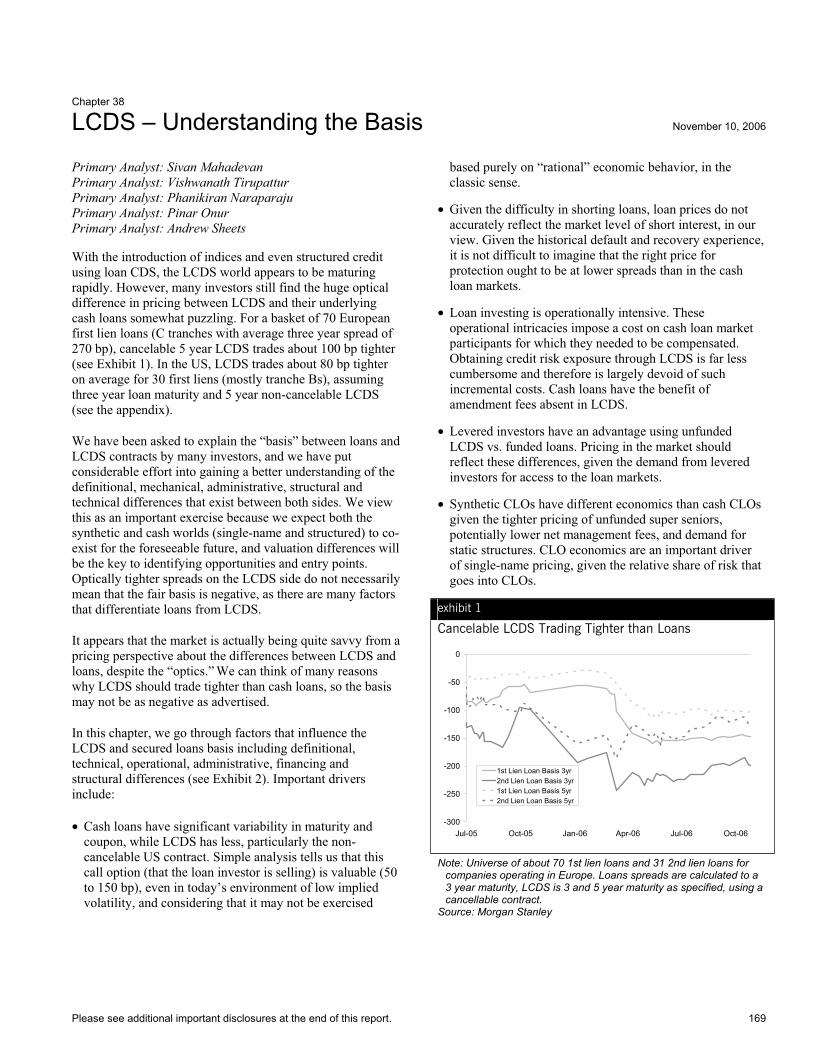
Please see additional important disclosures at the end of this report. 169
Chapter 38
LCDS – Understanding the Basis November 10, 2006
Primary Analyst: Sivan Mahadevan Primary Analyst: Vishwanath Tirupattur Primary Analyst: Phanikiran Naraparaju Primary Analyst: Pinar Onur Primary Analyst: Andrew Sheets
With the introduction of indices and even structured credit using loan CDS, the LCDS world appears to be maturing rapidly. However, many investors still find the huge optical difference in pricing between LCDS and their underlying cash loans somewhat puzzling. For a basket of 70 European first lien loans (C tranches with average three year spread of 270 bp), cancelable 5 year LCDS trades about 100 bp tighter (see Exhibit 1). In the US, LCDS trades about 80 bp tighter on average for 30 first liens (mostly tranche Bs), assuming three year loan maturity and 5 year non-cancelable LCDS (see the appendix).
We have been asked to explain the “basis” between loans and LCDS contracts by many investors, and we have put considerable effort into gaining a better understanding of the definitional, mechanical, administrative, structural and technical differences that exist between both sides. We view this as an important exercise because we expect both the synthetic and cash worlds (single-name and structured) to co-exist for the foreseeable future, and valuation differences will be the key to identifying opportunities and entry points. Optically tighter spreads on the LCDS side do not necessarily mean that the fair basis is negative, as there are many factors that differentiate loans from LCDS.
It appears that the market is actually being quite savvy from a pricing perspective about the differences between LCDS and loans, despite the “optics.” We can think of many reasons why LCDS should trade tighter than cash loans, so the basis may not be as negative as advertised.
In this chapter, we go through factors that influence the LCDS and secured loans basis including definitional, technical, operational, administrative, financing and structural differences (see Exhibit 2). Important drivers include:
• Cash loans have significant variability in maturity and coupon, while LCDS has less, particularly the non-cancelable US contract. Simple analysis tells us that this call option (that the loan investor is selling) is valuable (50 to 150 bp), even in today’s environment of low implied volatility, and considering that it may not be exercised
based purely on “rational” economic behavior, in the classic sense.
• Given the difficulty in shorting loans, loan prices do not accurately reflect the market level of short interest, in our view. Given the historical default and recovery experience, it is not difficult to imagine that the right price for protection ought to be at lower spreads than in the cash loan markets.
• Loan investing is operationally intensive. These operational intricacies impose a cost on cash loan market participants for which they needed to be compensated. Obtaining credit risk exposure through LCDS is far less cumbersome and therefore is largely devoid of such incremental costs. Cash loans have the benefit of amendment fees absent in LCDS.
• Levered investors have an advantage using unfunded LCDS vs. funded loans. Pricing in the market should reflect these differences, given the demand from levered investors for access to the loan markets.
• Synthetic CLOs have different economics than cash CLOs given the tighter pricing of unfunded super seniors, potentially lower net management fees, and demand for static structures. CLO economics are an important driver of single-name pricing, given the relative share of risk that goes into CLOs.
exhibit 1
Cancelable LCDS Trading Tighter than Loans
-300
-250
-200
-150
-100
-50
0
Jul-05 Oct-05 Jan-06 Apr-06 Jul-06 Oct-06
1st Lien Loan Basis 3yr2nd Lien Loan Basis 3yr1st Lien Loan Basis 5yr2nd Lien Loan Basis 5yr
Note: Universe of about 70 1st lien loans and 31 2nd lien loans for companies operating in Europe. Loans spreads are calculated to a 3 year maturity, LCDS is 3 and 5 year maturity as specified, using a cancellable contract.
Source: Morgan Stanley
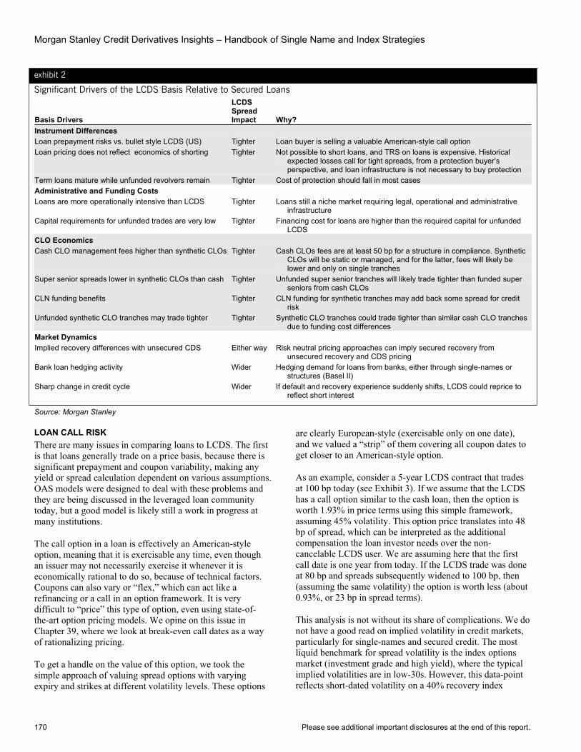
Morgan Stanley Credit Derivatives Insights – Handbook of Single Name and Index Strategies
170 Please see additional important disclosures at the end of this report.
exhibit 2
Significant Drivers of the LCDS Basis Relative to Secured Loans
Basis Drivers
LCDSSpreadImpact Why?
Instrument Differences Loan prepayment risks vs. bullet style LCDS (US) Tighter Loan buyer is selling a valuable American-style call option Loan pricing does not reflect economics of shorting Tighter Not possible to short loans, and TRS on loans is expensive. Historical
expected losses call for tight spreads, from a protection buyer’s perspective, and loan infrastructure is not necessary to buy protection
Term loans mature while unfunded revolvers remain Tighter Cost of protection should fall in most cases Administrative and Funding Costs Loans are more operationally intensive than LCDS Tighter Loans still a niche market requiring legal, operational and administrative
infrastructureCapital requirements for unfunded trades are very low Tighter Financing cost for loans are higher than the required capital for unfunded
LCDSCLO Economics Cash CLO management fees higher than synthetic CLOs Tighter Cash CLOs fees are at least 50 bp for a structure in compliance. Synthetic
CLOs will be static or managed, and for the latter, fees will likely be lower and only on single tranches
Super senior spreads lower in synthetic CLOs than cash Tighter Unfunded super senior tranches will likely trade tighter than funded super seniors from cash CLOs
CLN funding benefits Tighter CLN funding for synthetic tranches may add back some spread for credit risk
Unfunded synthetic CLO tranches may trade tighter Tighter Synthetic CLO tranches could trade tighter than similar cash CLO tranches due to funding cost differences
Market Dynamics Implied recovery differences with unsecured CDS Either way Risk neutral pricing approaches can imply secured recovery from
unsecured recovery and CDS pricing Bank loan hedging activity Wider Hedging demand for loans from banks, either through single-names or
structures (Basel II) Sharp change in credit cycle Wider If default and recovery experience suddenly shifts, LCDS could reprice to
reflect short interest
Source: Morgan Stanley
LOAN CALL RISK There are many issues in comparing loans to LCDS. The first is that loans generally trade on a price basis, because there is significant prepayment and coupon variability, making any yield or spread calculation dependent on various assumptions. OAS models were designed to deal with these problems and they are being discussed in the leveraged loan community today, but a good model is likely still a work in progress at many institutions.
The call option in a loan is effectively an American-style option, meaning that it is exercisable any time, even though an issuer may not necessarily exercise it whenever it is economically rational to do so, because of technical factors. Coupons can also vary or “flex,” which can act like a refinancing or a call in an option framework. It is very difficult to “price” this type of option, even using state-of-the-art option pricing models. We opine on this issue in Chapter 39, where we look at break-even call dates as a way of rationalizing pricing.
To get a handle on the value of this option, we took the simple approach of valuing spread options with varying expiry and strikes at different volatility levels. These options
are clearly European-style (exercisable only on one date), and we valued a “strip” of them covering all coupon dates to get closer to an American-style option.
As an example, consider a 5-year LCDS contract that trades at 100 bp today (see Exhibit 3). If we assume that the LCDS has a call option similar to the cash loan, then the option is worth 1.93% in price terms using this simple framework, assuming 45% volatility. This option price translates into 48 bp of spread, which can be interpreted as the additional compensation the loan investor needs over the non-cancelable LCDS user. We are assuming here that the first call date is one year from today. If the LCDS trade was done at 80 bp and spreads subsequently widened to 100 bp, then(assuming the same volatility) the option is worth less (about 0.93%, or 23 bp in spread terms).
This analysis is not without its share of complications. We do not have a good read on implied volatility in credit markets, particularly for single-names and secured credit. The most liquid benchmark for spread volatility is the index options market (investment grade and high yield), where the typical implied volatilities are in low-30s. However, this data-point reflects short-dated volatility on a 40% recovery index
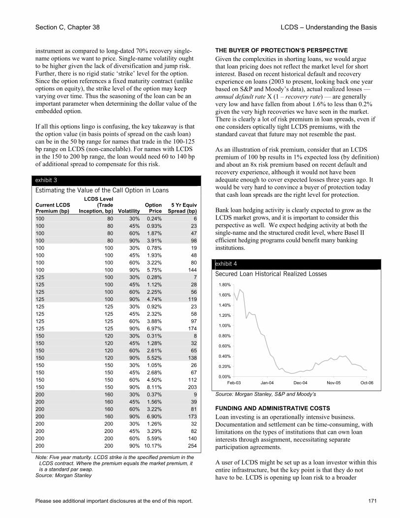
Section C, Chapter 38 LCDS – Understanding the Basis
Please see additional important disclosures at the end of this report. 171
instrument as compared to long-dated 70% recovery single-name options we want to price. Single-name volatility ought to be higher given the lack of diversification and jump risk. Further, there is no rigid static ‘strike’ level for the option. Since the option references a fixed maturity contract (unlike options on equity), the strike level of the option may keep varying over time. Thus the seasoning of the loan can be an important parameter when determining the dollar value of the embedded option.
If all this options lingo is confusing, the key takeaway is that the option value (in basis points of spread on the cash loan) can be in the 50 bp range for names that trade in the 100-125 bp range on LCDS (non-cancelable). For names with LCDS in the 150 to 200 bp range, the loan would need 60 to 140 bp of additional spread to compensate for this risk.
exhibit 3
Estimating the Value of the Call Option in Loans
Current LCDS Premium (bp)
LCDS Level (Trade
Inception, bp) Volatility Option
Price5 Yr Equiv
Spread (bp)100 80 30% 0.24% 6100 80 45% 0.93% 23100 80 60% 1.87% 47100 80 90% 3.91% 98100 100 30% 0.78% 19100 100 45% 1.93% 48100 100 60% 3.22% 80100 100 90% 5.75% 144125 100 30% 0.28% 7125 100 45% 1.12% 28125 100 60% 2.25% 56125 100 90% 4.74% 119125 125 30% 0.92% 23125 125 45% 2.32% 58125 125 60% 3.88% 97125 125 90% 6.97% 174150 120 30% 0.31% 8150 120 45% 1.28% 32150 120 60% 2.61% 65150 120 90% 5.52% 138150 150 30% 1.05% 26150 150 45% 2.68% 67150 150 60% 4.50% 112150 150 90% 8.11% 203200 160 30% 0.37% 9200 160 45% 1.56% 39200 160 60% 3.22% 81200 160 90% 6.90% 173200 200 30% 1.26% 32200 200 45% 3.29% 82200 200 60% 5.59% 140200 200 90% 10.17% 254
Note: Five year maturity. LCDS strike is the specified premium in the LCDS contract. Where the premium equals the market premium, it is a standard par swap.
Source: Morgan Stanley
THE BUYER OF PROTECTION’S PERSPECTIVE Given the complexities in shorting loans, we would argue that loan pricing does not reflect the market level for short interest. Based on recent historical default and recovery experience on loans (2003 to present, looking back one year based on S&P and Moody’s data), actual realized losses — annual default rate X (1 – recovery rate) — are generally very low and have fallen from about 1.6% to less than 0.2% given the very high recoveries we have seen in the market. There is clearly a lot of risk premium in loan spreads, even if one considers optically tight LCDS premiums, with the standard caveat that future may not resemble the past.
As an illustration of risk premium, consider that an LCDS premium of 100 bp results in 1% expected loss (by definition) and about an 8x risk premium based on recent default and recovery experience, although it would not have been adequate enough to cover expected losses three years ago. It would be very hard to convince a buyer of protection today that cash loan spreads are the right level for protection.
Bank loan hedging activity is clearly expected to grow as the LCDS market grows, and it is important to consider this perspective as well. We expect hedging activity at both the single-name and the structured credit level, where Basel II efficient hedging programs could benefit many banking institutions.
exhibit 4
Secured Loan Historical Realized Losses
0.00%
0.20%
0.40%
0.60%
0.80%
1.00%
1.20%
1.40%
1.60%
1.80%
Feb-03 Jan-04 Dec-04 Nov-05 Oct-06
Source: Morgan Stanley, S&P and Moody’s
FUNDING AND ADMINISTRATIVE COSTS Loan investing is an operationally intensive business. Documentation and settlement can be time-consuming, with limitations on the types of institutions that can own loan interests through assignment, necessitating separate participation agreements.
A user of LCDS might be set up as a loan investor within this entire infrastructure, but the key point is that they do not have to be. LCDS is opening up loan risk to a broader
Morgan Stanley Credit Derivatives Insights – Handbook of Single Name and Index Strategies
172 Please see additional important disclosures at the end of this report.
audience of investors, and only those who ultimately take delivery of loans physically would have to deal with some of these operational issues. This is another argument for LCDS trading tighter, all else being equal.
On the funding cost side, LCDS premiums are also affected by the nature of investors who seek access to the loan market. As a funded investment, loans require considerable capital compared to what counterparties require for selling protection using the LCDS contract. The fully funded (unlevered) investor might be indifferent to using loans versus LCDS, but for the large majority of loan participants who can use leverage, the difference is important, as funding costs for LCDS can be one-tenth that of other unfunded derivatives (like total return swaps referencing single term loans). Why is this issue not as prevalent in the unsecured investment grade and high yield markets? Simply put, unlevered investors are a much larger share of the investor pool in those markets than in loans.
CLO ECONOMICS CLOs account for two-thirds of the term loan activity in the US, and about 35% of it in Europe. Consequently, we argue that CLO capital structure and fee structure have an effect on the underlying loan spreads, so differences in cash and synthetic CLOs should matter as well.
Super senior AAA tranches account for about 75% of the CLO capital structure, pricing currently at about 25 bps. AAA tranches are usually placed using the so-called negative basis technology (where balance sheet providers take on the funded risk and buy unfunded protection on this risk at lower spreads from other investors, earning typically 8 to 10 bp in the process). The entire AAA tranche needs to be placed on a funded basis as long as the underlying CLO collateral is acquired in cash form. If a substantial part of the collateral is acquired through synthetic means, there could be a substantial unfunded senior/super senior tranche which would significantly improve the economics for the CLO capital structure, as unfunded super senior buyers can bypass the balance sheet providers. We argue that these inefficiencies of the fully funded capital structure in current cash CLOs are reflected in the cash loan spreads, since CLOs are such significant players in the cash loan market. By extension, the efficiencies that synthetic collateral would bring to CLO capital structure would also feed back in to the tighter LCDS spreads relative to cash loans.
Typical CLO manager fees are paid in three parts – about 20 bps of senior management fees at the top of the CLO cash flow waterfall, about 30 bps of junior management fees at the bottom of the waterfall, and incentive fees after the equity returns exceed an incentive fee hurdle. These manager fees are reflected in cash loan spreads in some form. Synthetic CLOs are likely to be static portfolios involving no manager — or they could be managed but with fees applied on a single-tranche basis, like we see in other single-tranche products. In either case, the overall manager fees are likely to be lower, which in our judgment should result in tighter LCDS spreads relative to cash loans.
The point here is that because of cash CLO funding “inefficiencies” and potentially higher embedded manager fees, they effectively impose a floor on cash loan spreads, i.e., if spreads tighten below some level, CLO economics won’t work and the CLO bid will back away. Since CLOs are such influential segment of the institutional term loan market, any such back-up will likely widen cash loan spreads. LCDS spreads don’t have a similar floor on their levels.
LCDS VS. LOANS – A WORLD OF DIFFERENCE The definitional, structural, operational and technical differences between LCDS and underlying secured loans are quite substantial, more so than we see in any other credit market where credit derivatives are active. As such the seemingly negative basis that we see in the market appears to be intuitively correct, even though the market is not yet ready to quantify it down to the basis point.
There are clearly a lot of technical forces that can keep LCDS premiums tight and push the optically negative basis into even more negative territory. Furthermore, protection buyers will demand low premiums in the current default and recovery environment. However, we caution that these relationships could change when the credit cycle ultimately turns, particularly if recovery experience is much lower than we have seen historically for secured loans. Could the basis change character at that time? We offer two points, both pointing to a less negative optical basis. First, at wider spreads, the call option loan investors are selling can be worth much less. Second, LCDS may widen more than cash loans in such an environment because this is the natural instrument to short loan risk. We have seen this behavior in investment grade markets over time (i.e., positive basis during times of stress).
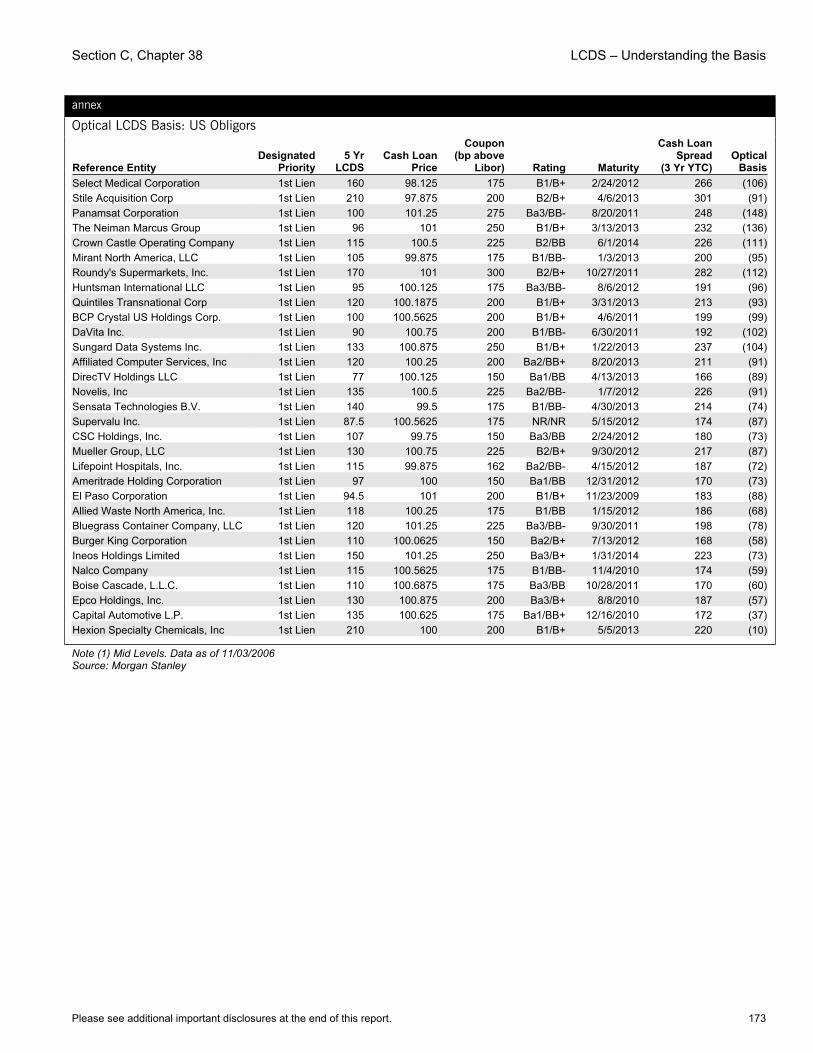
Section C, Chapter 38 LCDS – Understanding the Basis
Please see additional important disclosures at the end of this report. 173
annex
Optical LCDS Basis: US Obligors
Reference Entity Designated
Priority 5 Yr
LCDSCash Loan
Price
Coupon (bp above
Libor) Rating Maturity
Cash Loan Spread
(3 Yr YTC)Optical
BasisSelect Medical Corporation 1st Lien 160 98.125 175 B1/B+ 2/24/2012 266 (106)Stile Acquisition Corp 1st Lien 210 97.875 200 B2/B+ 4/6/2013 301 (91)Panamsat Corporation 1st Lien 100 101.25 275 Ba3/BB- 8/20/2011 248 (148)The Neiman Marcus Group 1st Lien 96 101 250 B1/B+ 3/13/2013 232 (136)Crown Castle Operating Company 1st Lien 115 100.5 225 B2/BB 6/1/2014 226 (111)Mirant North America, LLC 1st Lien 105 99.875 175 B1/BB- 1/3/2013 200 (95)Roundy's Supermarkets, Inc. 1st Lien 170 101 300 B2/B+ 10/27/2011 282 (112)Huntsman International LLC 1st Lien 95 100.125 175 Ba3/BB- 8/6/2012 191 (96)Quintiles Transnational Corp 1st Lien 120 100.1875 200 B1/B+ 3/31/2013 213 (93)BCP Crystal US Holdings Corp. 1st Lien 100 100.5625 200 B1/B+ 4/6/2011 199 (99)DaVita Inc. 1st Lien 90 100.75 200 B1/BB- 6/30/2011 192 (102)Sungard Data Systems Inc. 1st Lien 133 100.875 250 B1/B+ 1/22/2013 237 (104)Affiliated Computer Services, Inc 1st Lien 120 100.25 200 Ba2/BB+ 8/20/2013 211 (91)DirecTV Holdings LLC 1st Lien 77 100.125 150 Ba1/BB 4/13/2013 166 (89)Novelis, Inc 1st Lien 135 100.5 225 Ba2/BB- 1/7/2012 226 (91)Sensata Technologies B.V. 1st Lien 140 99.5 175 B1/BB- 4/30/2013 214 (74)Supervalu Inc. 1st Lien 87.5 100.5625 175 NR/NR 5/15/2012 174 (87)CSC Holdings, Inc. 1st Lien 107 99.75 150 Ba3/BB 2/24/2012 180 (73)Mueller Group, LLC 1st Lien 130 100.75 225 B2/B+ 9/30/2012 217 (87)Lifepoint Hospitals, Inc. 1st Lien 115 99.875 162 Ba2/BB- 4/15/2012 187 (72)Ameritrade Holding Corporation 1st Lien 97 100 150 Ba1/BB 12/31/2012 170 (73)El Paso Corporation 1st Lien 94.5 101 200 B1/B+ 11/23/2009 183 (88)Allied Waste North America, Inc. 1st Lien 118 100.25 175 B1/BB 1/15/2012 186 (68)Bluegrass Container Company, LLC 1st Lien 120 101.25 225 Ba3/BB- 9/30/2011 198 (78)Burger King Corporation 1st Lien 110 100.0625 150 Ba2/B+ 7/13/2012 168 (58)Ineos Holdings Limited 1st Lien 150 101.25 250 Ba3/B+ 1/31/2014 223 (73)Nalco Company 1st Lien 115 100.5625 175 B1/BB- 11/4/2010 174 (59)Boise Cascade, L.L.C. 1st Lien 110 100.6875 175 Ba3/BB 10/28/2011 170 (60)Epco Holdings, Inc. 1st Lien 130 100.875 200 Ba3/B+ 8/8/2010 187 (57)Capital Automotive L.P. 1st Lien 135 100.625 175 Ba1/BB+ 12/16/2010 172 (37)Hexion Specialty Chemicals, Inc 1st Lien 210 100 200 B1/B+ 5/5/2013 220 (10)
Note (1) Mid Levels. Data as of 11/03/2006 Source: Morgan Stanley
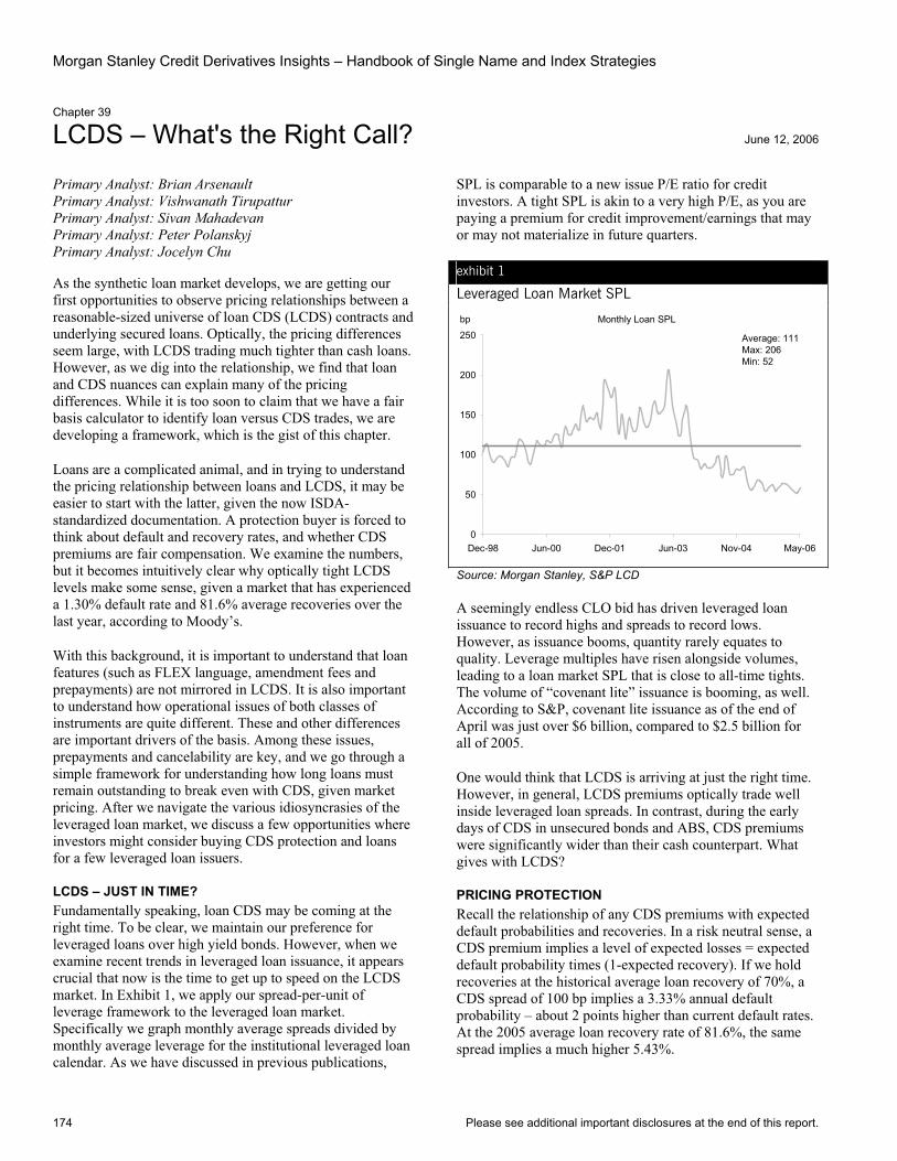
Morgan Stanley Credit Derivatives Insights – Handbook of Single Name and Index Strategies
174 Please see additional important disclosures at the end of this report.
Chapter 39
LCDS – What's the Right Call? June 12, 2006
Primary Analyst: Brian Arsenault Primary Analyst: Vishwanath Tirupattur Primary Analyst: Sivan Mahadevan Primary Analyst: Peter Polanskyj Primary Analyst: Jocelyn Chu
As the synthetic loan market develops, we are getting our first opportunities to observe pricing relationships between a reasonable-sized universe of loan CDS (LCDS) contracts and underlying secured loans. Optically, the pricing differences seem large, with LCDS trading much tighter than cash loans. However, as we dig into the relationship, we find that loan and CDS nuances can explain many of the pricing differences. While it is too soon to claim that we have a fair basis calculator to identify loan versus CDS trades, we are developing a framework, which is the gist of this chapter.
Loans are a complicated animal, and in trying to understand the pricing relationship between loans and LCDS, it may be easier to start with the latter, given the now ISDA-standardized documentation. A protection buyer is forced to think about default and recovery rates, and whether CDS premiums are fair compensation. We examine the numbers, but it becomes intuitively clear why optically tight LCDS levels make some sense, given a market that has experienced a 1.30% default rate and 81.6% average recoveries over the last year, according to Moody’s.
With this background, it is important to understand that loan features (such as FLEX language, amendment fees and prepayments) are not mirrored in LCDS. It is also important to understand how operational issues of both classes of instruments are quite different. These and other differences are important drivers of the basis. Among these issues, prepayments and cancelability are key, and we go through a simple framework for understanding how long loans must remain outstanding to break even with CDS, given market pricing. After we navigate the various idiosyncrasies of the leveraged loan market, we discuss a few opportunities where investors might consider buying CDS protection and loans for a few leveraged loan issuers.
LCDS – JUST IN TIME? Fundamentally speaking, loan CDS may be coming at the right time. To be clear, we maintain our preference for leveraged loans over high yield bonds. However, when we examine recent trends in leveraged loan issuance, it appears crucial that now is the time to get up to speed on the LCDS market. In Exhibit 1, we apply our spread-per-unit of leverage framework to the leveraged loan market. Specifically we graph monthly average spreads divided by monthly average leverage for the institutional leveraged loan calendar. As we have discussed in previous publications,
SPL is comparable to a new issue P/E ratio for credit investors. A tight SPL is akin to a very high P/E, as you are paying a premium for credit improvement/earnings that may or may not materialize in future quarters.
exhibit 1
Leveraged Loan Market SPL
Monthly Loan SPL
0
50
100
150
200
250
Dec-98 Jun-00 Dec-01 Jun-03 Nov-04 May-06
bp
Average: 111Max: 206Min: 52
Source: Morgan Stanley, S&P LCD
A seemingly endless CLO bid has driven leveraged loan issuance to record highs and spreads to record lows. However, as issuance booms, quantity rarely equates to quality. Leverage multiples have risen alongside volumes, leading to a loan market SPL that is close to all-time tights. The volume of “covenant lite” issuance is booming, as well. According to S&P, covenant lite issuance as of the end of April was just over $6 billion, compared to $2.5 billion for all of 2005.
One would think that LCDS is arriving at just the right time. However, in general, LCDS premiums optically trade well inside leveraged loan spreads. In contrast, during the early days of CDS in unsecured bonds and ABS, CDS premiums were significantly wider than their cash counterpart. What gives with LCDS?
PRICING PROTECTION Recall the relationship of any CDS premiums with expected default probabilities and recoveries. In a risk neutral sense, a CDS premium implies a level of expected losses = expected default probability times (1-expected recovery). If we hold recoveries at the historical average loan recovery of 70%, a CDS spread of 100 bp implies a 3.33% annual default probability – about 2 points higher than current default rates. At the 2005 average loan recovery rate of 81.6%, the same spread implies a much higher 5.43%.
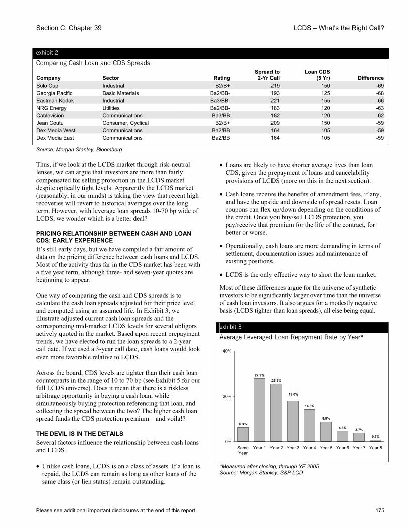
Section C, Chapter 39 LCDS – What's the Right Call?
Please see additional important disclosures at the end of this report. 175
exhibit 2
Comparing Cash Loan and CDS Spreads
Company Sector RatingSpread to
2-Yr CallLoan CDS
(5 Yr) DifferenceSolo Cup Industrial B2/B+ 219 150 -69Georgia Pacific Basic Materials Ba2/BB- 193 125 -68Eastman Kodak Industrial Ba3/BB- 221 155 -66NRG Energy Utilities Ba2/BB- 183 120 -63Cablevision Communications Ba3/BB 182 120 -62Jean Coutu Consumer, Cyclical B2/B+ 209 150 -59Dex Media West Communications Ba2/BB 164 105 -59Dex Media East Communications Ba2/BB 164 105 -59
Source: Morgan Stanley, Bloomberg
Thus, if we look at the LCDS market through risk-neutral lenses, we can argue that investors are more than fairly compensated for selling protection in the LCDS market despite optically tight levels. Apparently the LCDS market (reasonably, in our minds) is taking the view that recent high recoveries will revert to historical averages over the long term. However, with leverage loan spreads 10-70 bp wide of LCDS, we wonder which is a better deal?
PRICING RELATIONSHIP BETWEEN CASH AND LOAN CDS: EARLY EXPERIENCE It’s still early days, but we have compiled a fair amount of data on the pricing difference between cash loans and LCDS. Most of the activity thus far in the CDS market has been with a five year term, although three- and seven-year quotes are beginning to appear.
One way of comparing the cash and CDS spreads is to calculate the cash loan spreads adjusted for their price level and computed using an assumed life. In Exhibit 3, we illustrate adjusted current cash loan spreads and the corresponding mid-market LCDS levels for several obligors actively quoted in the market. Based upon recent prepayment trends, we have elected to run the loan spreads to a 2-year call date. If we used a 3-year call date, cash loans would look even more favorable relative to LCDS.
Across the board, CDS levels are tighter than their cash loan counterparts in the range of 10 to 70 bp (see Exhibit 5 for our full LCDS universe). Does it mean that there is a riskless arbitrage opportunity in buying a cash loan, while simultaneously buying protection referencing that loan, and collecting the spread between the two? The higher cash loan spread funds the CDS protection premium – and voila!?
THE DEVIL IS IN THE DETAILS Several factors influence the relationship between cash loans and LCDS.
• Unlike cash loans, LCDS is on a class of assets. If a loan is repaid, the LCDS can remain as long as other loans of the same class (or lien status) remain outstanding.
• Loans are likely to have shorter average lives than loan CDS, given the prepayment of loans and cancelability provisions of LCDS (more on this in the next section).
• Cash loans receive the benefits of amendment fees, if any, and have the upside and downside of spread resets. Loan coupons can flex up/down depending on the conditions of the credit. Once you buy/sell LCDS protection, you pay/receive that premium for the life of the contract, for better or worse.
• Operationally, cash loans are more demanding in terms of settlement, documentation issues and maintenance of existing positions.
• LCDS is the only effective way to short the loan market.
Most of these differences argue for the universe of synthetic investors to be significantly larger over time than the universe of cash loan investors. It also argues for a modestly negative basis (LCDS tighter than loan spreads), all else being equal.
exhibit 3
Average Leveraged Loan Repayment Rate by Year*
6.3%
27.9%25.5%
14.3%
8.8%
4.6% 3.7%
0.7%
18.0%
0%
20%
40%
SameYear
Year 1 Year 2 Year 3 Year 4 Year 5 Year 6 Year 7 Year 8
*Measured after closing; through YE 2005 Source: Morgan Stanley, S&P LCD
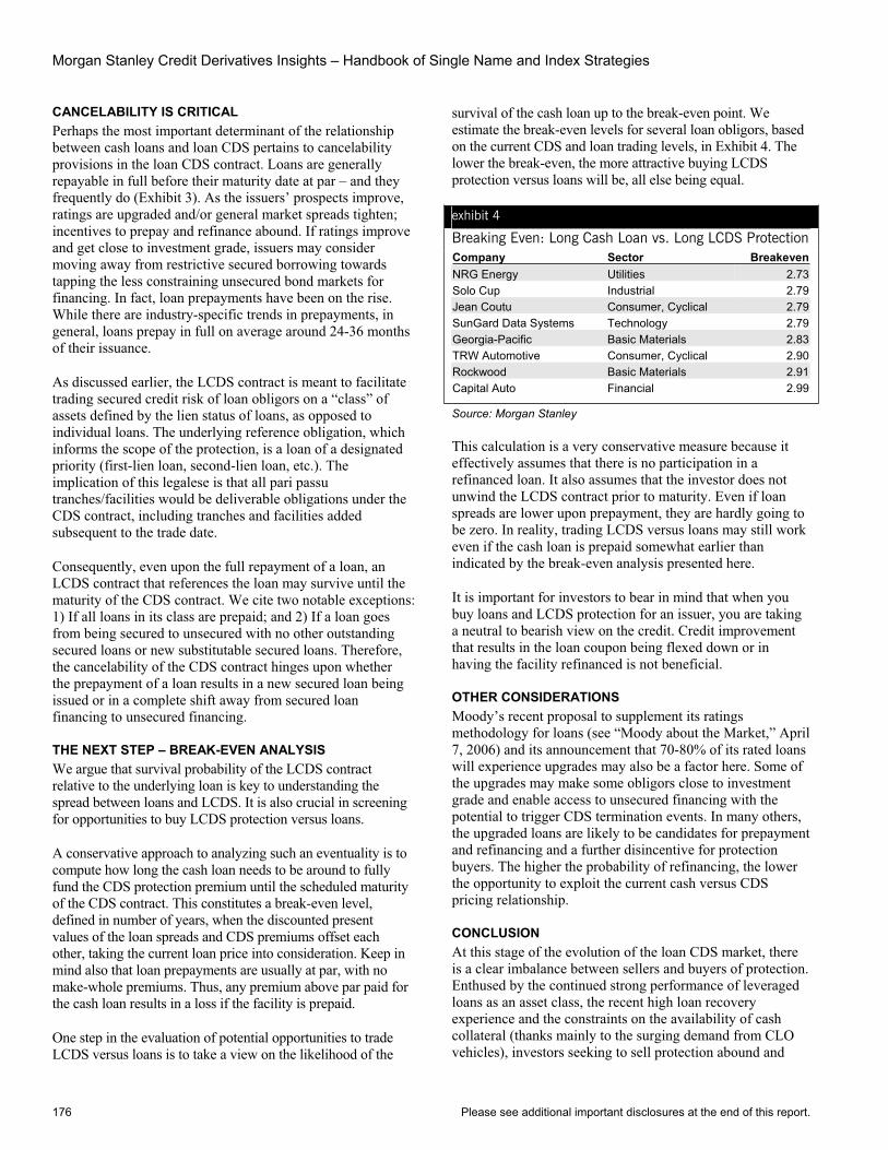
Morgan Stanley Credit Derivatives Insights – Handbook of Single Name and Index Strategies
176 Please see additional important disclosures at the end of this report.
CANCELABILITY IS CRITICAL Perhaps the most important determinant of the relationship between cash loans and loan CDS pertains to cancelability provisions in the loan CDS contract. Loans are generally repayable in full before their maturity date at par – and they frequently do (Exhibit 3). As the issuers’ prospects improve, ratings are upgraded and/or general market spreads tighten; incentives to prepay and refinance abound. If ratings improve and get close to investment grade, issuers may consider moving away from restrictive secured borrowing towards tapping the less constraining unsecured bond markets for financing. In fact, loan prepayments have been on the rise. While there are industry-specific trends in prepayments, in general, loans prepay in full on average around 24-36 months of their issuance.
As discussed earlier, the LCDS contract is meant to facilitate trading secured credit risk of loan obligors on a “class” of assets defined by the lien status of loans, as opposed to individual loans. The underlying reference obligation, which informs the scope of the protection, is a loan of a designated priority (first-lien loan, second-lien loan, etc.). The implication of this legalese is that all pari passu tranches/facilities would be deliverable obligations under the CDS contract, including tranches and facilities added subsequent to the trade date.
Consequently, even upon the full repayment of a loan, an LCDS contract that references the loan may survive until the maturity of the CDS contract. We cite two notable exceptions: 1) If all loans in its class are prepaid; and 2) If a loan goes from being secured to unsecured with no other outstanding secured loans or new substitutable secured loans. Therefore, the cancelability of the CDS contract hinges upon whether the prepayment of a loan results in a new secured loan being issued or in a complete shift away from secured loan financing to unsecured financing.
THE NEXT STEP – BREAK-EVEN ANALYSIS We argue that survival probability of the LCDS contract relative to the underlying loan is key to understanding the spread between loans and LCDS. It is also crucial in screening for opportunities to buy LCDS protection versus loans.
A conservative approach to analyzing such an eventuality is to compute how long the cash loan needs to be around to fully fund the CDS protection premium until the scheduled maturity of the CDS contract. This constitutes a break-even level, defined in number of years, when the discounted present values of the loan spreads and CDS premiums offset each other, taking the current loan price into consideration. Keep in mind also that loan prepayments are usually at par, with no make-whole premiums. Thus, any premium above par paid for the cash loan results in a loss if the facility is prepaid.
One step in the evaluation of potential opportunities to trade LCDS versus loans is to take a view on the likelihood of the
survival of the cash loan up to the break-even point. We estimate the break-even levels for several loan obligors, based on the current CDS and loan trading levels, in Exhibit 4. The lower the break-even, the more attractive buying LCDS protection versus loans will be, all else being equal.
exhibit 4
Breaking Even: Long Cash Loan vs. Long LCDS Protection Company Sector BreakevenNRG Energy Utilities 2.73Solo Cup Industrial 2.79Jean Coutu Consumer, Cyclical 2.79SunGard Data Systems Technology 2.79Georgia-Pacific Basic Materials 2.83TRW Automotive Consumer, Cyclical 2.90Rockwood Basic Materials 2.91Capital Auto Financial 2.99
Source: Morgan Stanley
This calculation is a very conservative measure because it effectively assumes that there is no participation in a refinanced loan. It also assumes that the investor does not unwind the LCDS contract prior to maturity. Even if loan spreads are lower upon prepayment, they are hardly going to be zero. In reality, trading LCDS versus loans may still work even if the cash loan is prepaid somewhat earlier than indicated by the break-even analysis presented here.
It is important for investors to bear in mind that when you buy loans and LCDS protection for an issuer, you are taking a neutral to bearish view on the credit. Credit improvement that results in the loan coupon being flexed down or in having the facility refinanced is not beneficial.
OTHER CONSIDERATIONS Moody’s recent proposal to supplement its ratings methodology for loans (see “Moody about the Market,” April 7, 2006) and its announcement that 70-80% of its rated loans will experience upgrades may also be a factor here. Some of the upgrades may make some obligors close to investment grade and enable access to unsecured financing with the potential to trigger CDS termination events. In many others, the upgraded loans are likely to be candidates for prepayment and refinancing and a further disincentive for protection buyers. The higher the probability of refinancing, the lower the opportunity to exploit the current cash versus CDS pricing relationship.
CONCLUSIONAt this stage of the evolution of the loan CDS market, there is a clear imbalance between sellers and buyers of protection. Enthused by the continued strong performance of leveraged loans as an asset class, the recent high loan recovery experience and the constraints on the availability of cash collateral (thanks mainly to the surging demand from CLO vehicles), investors seeking to sell protection abound and
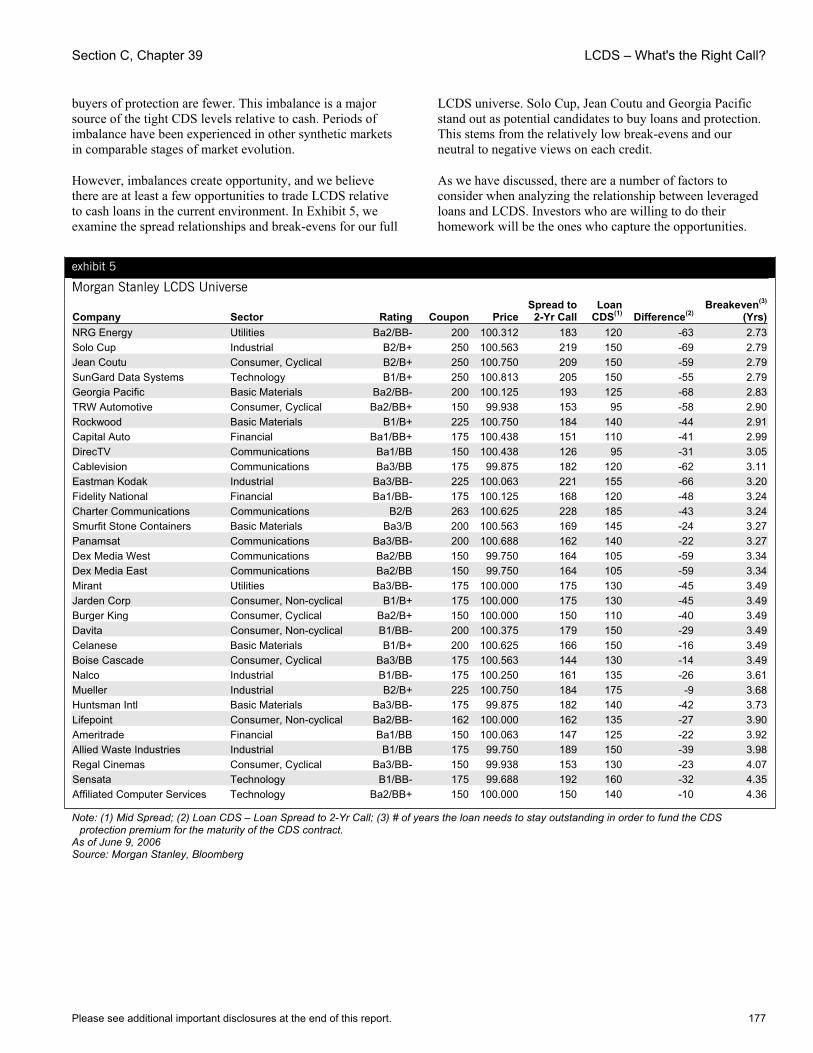
Section C, Chapter 39 LCDS – What's the Right Call?
Please see additional important disclosures at the end of this report. 177
buyers of protection are fewer. This imbalance is a major source of the tight CDS levels relative to cash. Periods of imbalance have been experienced in other synthetic markets in comparable stages of market evolution.
However, imbalances create opportunity, and we believe there are at least a few opportunities to trade LCDS relative to cash loans in the current environment. In Exhibit 5, we examine the spread relationships and break-evens for our full
LCDS universe. Solo Cup, Jean Coutu and Georgia Pacific stand out as potential candidates to buy loans and protection. This stems from the relatively low break-evens and our neutral to negative views on each credit.
As we have discussed, there are a number of factors to consider when analyzing the relationship between leveraged loans and LCDS. Investors who are willing to do their homework will be the ones who capture the opportunities.
exhibit 5
Morgan Stanley LCDS Universe
Company Sector Rating Coupon PriceSpread to
2-Yr Call Loan
CDS(1) Difference(2)Breakeven(3)
(Yrs)NRG Energy Utilities Ba2/BB- 200 100.312 183 120 -63 2.73Solo Cup Industrial B2/B+ 250 100.563 219 150 -69 2.79Jean Coutu Consumer, Cyclical B2/B+ 250 100.750 209 150 -59 2.79SunGard Data Systems Technology B1/B+ 250 100.813 205 150 -55 2.79Georgia Pacific Basic Materials Ba2/BB- 200 100.125 193 125 -68 2.83TRW Automotive Consumer, Cyclical Ba2/BB+ 150 99.938 153 95 -58 2.90Rockwood Basic Materials B1/B+ 225 100.750 184 140 -44 2.91Capital Auto Financial Ba1/BB+ 175 100.438 151 110 -41 2.99DirecTV Communications Ba1/BB 150 100.438 126 95 -31 3.05Cablevision Communications Ba3/BB 175 99.875 182 120 -62 3.11Eastman Kodak Industrial Ba3/BB- 225 100.063 221 155 -66 3.20Fidelity National Financial Ba1/BB- 175 100.125 168 120 -48 3.24Charter Communications Communications B2/B 263 100.625 228 185 -43 3.24Smurfit Stone Containers Basic Materials Ba3/B 200 100.563 169 145 -24 3.27Panamsat Communications Ba3/BB- 200 100.688 162 140 -22 3.27Dex Media West Communications Ba2/BB 150 99.750 164 105 -59 3.34Dex Media East Communications Ba2/BB 150 99.750 164 105 -59 3.34Mirant Utilities Ba3/BB- 175 100.000 175 130 -45 3.49Jarden Corp Consumer, Non-cyclical B1/B+ 175 100.000 175 130 -45 3.49Burger King Consumer, Cyclical Ba2/B+ 150 100.000 150 110 -40 3.49Davita Consumer, Non-cyclical B1/BB- 200 100.375 179 150 -29 3.49Celanese Basic Materials B1/B+ 200 100.625 166 150 -16 3.49Boise Cascade Consumer, Cyclical Ba3/BB 175 100.563 144 130 -14 3.49Nalco Industrial B1/BB- 175 100.250 161 135 -26 3.61Mueller Industrial B2/B+ 225 100.750 184 175 -9 3.68Huntsman Intl Basic Materials Ba3/BB- 175 99.875 182 140 -42 3.73Lifepoint Consumer, Non-cyclical Ba2/BB- 162 100.000 162 135 -27 3.90Ameritrade Financial Ba1/BB 150 100.063 147 125 -22 3.92Allied Waste Industries Industrial B1/BB 175 99.750 189 150 -39 3.98Regal Cinemas Consumer, Cyclical Ba3/BB- 150 99.938 153 130 -23 4.07Sensata Technology B1/BB- 175 99.688 192 160 -32 4.35Affiliated Computer Services Technology Ba2/BB+ 150 100.000 150 140 -10 4.36
Note: (1) Mid Spread; (2) Loan CDS – Loan Spread to 2-Yr Call; (3) # of years the loan needs to stay outstanding in order to fund the CDS protection premium for the maturity of the CDS contract.
As of June 9, 2006 Source: Morgan Stanley, Bloomberg
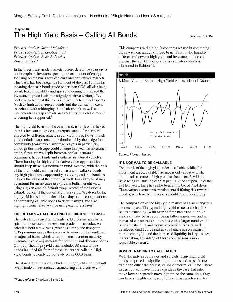
Morgan Stanley Credit Derivatives Insights – Handbook of Single Name and Index Strategies
178 Please see additional important disclosures at the end of this report.
Chapter 40
The High Yield Basis – Calling All Bonds February 6, 2004
Primary Analyst: Sivan Mahadevan Primary Analyst: Brian Arsenault Primary Analyst: Peter Polanskyj Anisha Ambardar
In the investment grade markets, where default swap usage is commonplace, investors spend quite an amount of energy focusing on the basis between cash and derivatives markets. This basis has been negative for most of the past 15 months, meaning that cash bonds trade wider than CDS, all else being equal. Recent volatility and spread widening has moved the investment grade basis into slightly positive territory. We continue to feel that this basis is driven by technical aspects (such as high dollar-priced bonds and the transaction costs associated with arbitraging the relationship), as well as movements in swap spreads and volatility, which the recent widening has supported.1
The high yield basis, on the other hand, is far less trafficked than its investment grade counterpart, and is furthermore affected by different issues, in our view. First, flows in high yield default swaps tend to be dominated by the hedge fund community (convertible arbitrage players in particular), although this landscape could change this year. In investment grade, flows are well split between banks, insurance companies, hedge funds and synthetic structured vehicles. Those hunting for high yield relative value opportunities should keep these distinctions in mind. Second, with the bulk of the high yield cash market consisting of callable bonds, any high yield basis opportunity involving callable bonds is a play on the value of the option, as well. For example, it may be natural for an investor to express a bullish credit view using a given credit’s default swap instead of the issuer’s callable bonds, if the option itself has value. We describe the high yield basis in more detail focusing on the complications of comparing callable bonds to default swaps. We also highlight some relative value using example issuers.
THE DETAILS – CALCULATING THE HIGH YIELD BASIS The calculations used in the high yield basis are similar, in spirit, to those used in investment grade. In particular, we calculate both a raw basis (which is simply the five-year CDS premium minus the Z-spread to worst of the bond) and an adjusted basis, which takes into consideration maturity mismatches and adjustments for premium and discount bonds. Our published high yield basis includes 38 issuers. The bonds included for four of these issuers are callable. High yield bonds typically do not trade on an OAS basis.
The standard terms under which US high yield credit default swaps trade do not include restructuring as a credit event.
1Please refer to Chapters 15 and 35.
This compares to the Mod R contracts we use in computing the investment grade synthetic basis. Finally, the liquidity differences between high yield and investment grade can increase the volatility of our basis estimates (which is illustrated in Exhibit 1).
exhibit 1
A More Volatile Basis – High Yield vs. Investment Grade
-45
-35
-25
-15
-5
5
15
Aug-03 Sep-03 Oct-03 Nov-03 Dec-03 Jan-04 Feb-04
High Yield Ex-AirlinesInvestment Grade
Source: Morgan Stanley
IT’S NORMAL TO BE CALLABLE Two-thirds of the high yield index is callable, while, for investment grade, callable issuance is only about 4%. The traditional structure in high yield has been 10nc5, with the issue being callable in year 5 at par + 1/2 the coupon. Over the last few years, there have also been a number of 7nc4 deals. These variable structures translate into differing risk reward profiles, which we feel investors should consider carefully.
The composition of the high yield market has also changed in the recent past. The typical high yield issuer once had 2-3 issues outstanding. With over half the names on our high yield synthetic basis report being fallen angels, we find an increased concentration of credits with a larger number of issues outstanding and extensive credit curves. A well developed credit curve makes synthetic-cash comparison more meaningful, and the increased liquidity in large issues makes taking advantage of these comparisons a more reasonable exercise.
BONDS TRADING TO CALL DATES With the rally in both rates and spreads, many high yield bonds are priced at significant premiums and, as such, are trading to either the nearest, or some interim, call date. These issues now can have limited upside in the case that rates move lower or spreads move tighter. At the same time, they can have a heightened susceptibility to rising interest rates.
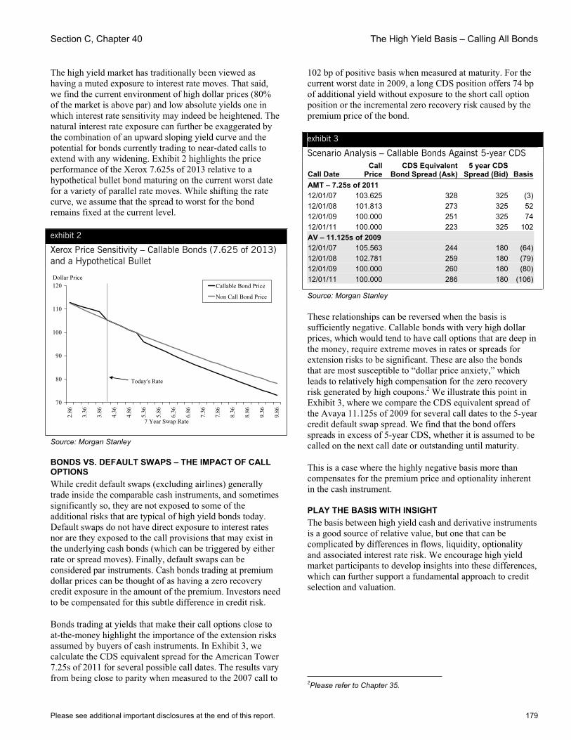
Section C, Chapter 40 The High Yield Basis – Calling All Bonds
Please see additional important disclosures at the end of this report. 179
The high yield market has traditionally been viewed as having a muted exposure to interest rate moves. That said, we find the current environment of high dollar prices (80% of the market is above par) and low absolute yields one in which interest rate sensitivity may indeed be heightened. The natural interest rate exposure can further be exaggerated by the combination of an upward sloping yield curve and the potential for bonds currently trading to near-dated calls to extend with any widening. Exhibit 2 highlights the price performance of the Xerox 7.625s of 2013 relative to a hypothetical bullet bond maturing on the current worst date for a variety of parallel rate moves. While shifting the rate curve, we assume that the spread to worst for the bond remains fixed at the current level.
exhibit 2
Xerox Price Sensitivity – Callable Bonds (7.625 of 2013) and a Hypothetical Bullet
Dollar Price
70
80
90
100
110
120
2.86
3.36
3.86
4.36
4.86
5.36
5.86
6.36
6.86
7.36
7.86
8.36
8.86
9.36
9.86
7 Year Swap Rate
Callable Bond Price
Non Call Bond Price
Today's Rate
Source: Morgan Stanley
BONDS VS. DEFAULT SWAPS – THE IMPACT OF CALL OPTIONSWhile credit default swaps (excluding airlines) generally trade inside the comparable cash instruments, and sometimes significantly so, they are not exposed to some of the additional risks that are typical of high yield bonds today. Default swaps do not have direct exposure to interest rates nor are they exposed to the call provisions that may exist in the underlying cash bonds (which can be triggered by either rate or spread moves). Finally, default swaps can be considered par instruments. Cash bonds trading at premium dollar prices can be thought of as having a zero recovery credit exposure in the amount of the premium. Investors need to be compensated for this subtle difference in credit risk.
Bonds trading at yields that make their call options close to at-the-money highlight the importance of the extension risks assumed by buyers of cash instruments. In Exhibit 3, we calculate the CDS equivalent spread for the American Tower 7.25s of 2011 for several possible call dates. The results vary from being close to parity when measured to the 2007 call to
102 bp of positive basis when measured at maturity. For the current worst date in 2009, a long CDS position offers 74 bp of additional yield without exposure to the short call option position or the incremental zero recovery risk caused by the premium price of the bond.
exhibit 3
Scenario Analysis – Callable Bonds Against 5-year CDS
Call Date Call
PriceCDS Equivalent
Bond Spread (Ask) 5 year CDS
Spread (Bid) BasisAMT – 7.25s of 2011 12/01/07 103.625 328 325 (3)12/01/08 101.813 273 325 52 12/01/09 100.000 251 325 74 12/01/11 100.000 223 325 102 AV – 11.125s of 2009 12/01/07 105.563 244 180 (64)12/01/08 102.781 259 180 (79)12/01/09 100.000 260 180 (80)12/01/11 100.000 286 180 (106)
Source: Morgan Stanley
These relationships can be reversed when the basis is sufficiently negative. Callable bonds with very high dollar prices, which would tend to have call options that are deep in the money, require extreme moves in rates or spreads for extension risks to be significant. These are also the bonds that are most susceptible to “dollar price anxiety,” which leads to relatively high compensation for the zero recovery risk generated by high coupons.2 We illustrate this point in Exhibit 3, where we compare the CDS equivalent spread of the Avaya 11.125s of 2009 for several call dates to the 5-year credit default swap spread. We find that the bond offers spreads in excess of 5-year CDS, whether it is assumed to be called on the next call date or outstanding until maturity.
This is a case where the highly negative basis more than compensates for the premium price and optionality inherent in the cash instrument.
PLAY THE BASIS WITH INSIGHT The basis between high yield cash and derivative instruments is a good source of relative value, but one that can be complicated by differences in flows, liquidity, optionality and associated interest rate risk. We encourage high yield market participants to develop insights into these differences, which can further support a fundamental approach to credit selection and valuation.
2Please refer to Chapter 35.

Morgan Stanley Credit Derivatives Insights – Handbook of Single Name and Index Strategies
180 Please see additional important disclosures at the end of this report.
Chapter 41
High Yield, Higher Rates, Hello Convexity June 18, 2004
Primary Analyst: Sivan Mahadevan Primary Analyst: Peter Polanskyj Primary Analyst: Brian Arsenault Anisha Ambardar Angira Apte
In investment grade markets, we have discussed in detail the drivers behind the regime shift in the basis (between cash and default swaps), which we argue is related to both interest rate moves and a “cultural” difference in flows. Corporate bond investors, many of whom run portfolios versus credit benchmarks or liabilities, have supported spreads this year, while many in the levered investment community have feared the impact that rising rates may have on credit, and have subsequently lightened up long exposures, established shorts, or left the markets altogether. The result is that default swaps have traded comfortably wider than corporate bonds over the past few months, after having been the other way around for almost 18 months.1
The high yield basis is a much harder relationship to generalize, but we do find some similar themes playing out in this more levered corner of the credit markets. On the surface, the high yield basis has widened out into positive territory as well, although much more recently than in the investment grade markets (see Exhibit 1). Like investment grade, traditional cash investors are continuing to stay long the market and support spreads, while hedge funds have reduced long credit positions in default swaps. Yet, the rise in interest rates has had a more important impact on high yield. With well over half the market comprised of callable bonds, the high yield index has extended in maturity (to worst) by six months, driven by an average extension of 2.3 years for the more than 250 bonds in the index that actually changed “to-worst” dates over the past two months.
We believe that high yield callable bond investors have not been adequately compensated for extension risk, as implied by prices on default swaps or bullet bonds.2 With the rise in rates, we find that, for many callable bonds where implied option prices were small or non-existent, price performance was much worse than for the market at large.
Furthermore, despite a wider basis, we find the current environment in high yield to be attractive for asymmetry (or “convexity”) trades, where an investor positions a discount-priced long-dated bond relative to shorter-dated protection to implement a convex pay-off profile for big moves in the credit (in either direction).
1Please refer to “Reacting to the New Regime,” Credit Derivatives Insights, May 14, 2004. 2Please refer to Chapter 61.
exhibit 1
Comparing the Basis – High Yield Catches Up to and Passes Investment Grade
-50
-40
-30
-20
-10
0
10
20
30
Aug-03 Oct-03 Dec-03 Feb-04 Apr-04 Jun-04
HY Basis (ex-Airlines)IG Basis
Source: Morgan Stanley
HIGH YIELD REACTS TO THE NEW REGIME The rise in rates and reshaping of the Treasury curve has caused the high yield index to extend in maturity (to-worst date) by six months since the end of March, on average. Yet, since averages are not always the best way to describe the high yield market, the details are important. Out of 1,237 index bonds, 266 (22%) actually extended, meaning that they now trade to a call date that is further out (or to maturity). The average extension among these bonds was 2.3 years, with half of them (11% of the market) extending by more than two years. Who said high yield does not have interest rate risk?
exhibit 2
High Yield Market Reacting to Interest Rate Moves High Yield Index Bonds that Actually Extended Maturity
(to Worst)Duration
(to Worst) Price Maturity (to Worst)
Duration (to Worst) Price
2-Month Average Change(Market Weighted) 0.5 yrs 0.0 yrs -3.6 pts 2.3 yrs 0.9 yrs -3.8 pts2-Month MedianChange(NotWeighted) 0.0 yrs -0.2 yrs -3.1 pts 2.0 yrs 1.0 yrs -4.0 pts
Source: Morgan Stanley, Salomon Analytics
Spreads to Libor have moved 15 bp tighter since the end of March, but we caution that Z-spread measures should tighten when dollar prices fall, all else being equal. The average price of the index has dropped by 3.6 points over this two-month period. For the bonds that extended, the average price fall was
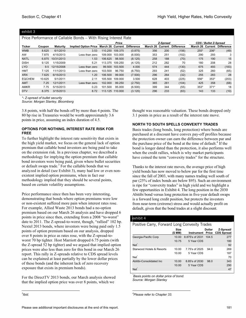
Section C, Chapter 41 High Yield, Higher Rates, Hello Convexity
Please see additional important disclosures at the end of this report. 181
exhibit 3
Price Performance of Callable Bonds – With Rising Interest Rate Price Z-Spread CDS / Bullet Z-Spread
Ticker Coupon Maturity Implied Option Price March 26 Current Difference March 26 Current Difference March 26 Current DifferenceWMB 8.625 6/1/2010 3.53 110.250 109.375 (0.875) 356 200 (156) 255* 206* (49)AW 7.875 4/15/2013 Less than zero 109.000 103.000 (6.000) 353 251 (102) 290 293 3NXTL 6.875 10/31/2013 1.53 106.625 98.500 (8.125) 258 188 (70) 175 190 15DISH 9.125 1/15/2009 5.21 113.375 109.250 (4.125) 212 282 70 180 208 28LYO 9.5 12/15/2008 Less than zero 99.500 103.500 4.000 574 444 (130) 675 493 (183)HMT 7.125 11/1/2013 Less than zero 103.500 96.750 (6.750) 293 241 (52) 325 260 (65)XRX 7.625 6/15/2013 1.20 106.500 99.000 (7.500) 296 264 (32) 255 283 28EQCHEM 10.625 5/1/2011 2.11 105.500 109.000 3.500 628 403 (225) 556* 353* (203)AMT 7.25 12/1/2011 Less than zero 102.000 99.250 (2.750) 365 261 (104) 425 358 (68)AMKR 7.75 5/15/2013 0.23 101.500 95.000 (6.500) 399 344 (55) 353* 371* 18DTV 8.375 3/15/2013 8.72 113.125 110.000 (3.120) 296 233 (63) 143 133 (10)
*- Z-spread of bullet security Source: Morgan Stanley, Bloomberg
3.8 points, with half the bonds off by more than 4 points. The 80 bp rise in Treasuries would be worth approximately 3.6 points in price, assuming an index duration of 4.5.
OPTIONS FOR NOTHING, INTEREST RATE RISK FOR FREETo further highlight the interest rate sensitivity that exists in the high yield market, we focus on the general lack of option premium that callable bond investors are being paid to take on the extension risk. In a previous chapter, we described a methodology for implying the option premium that callable bond investors were being paid, given where bullet securities or default swaps trade.3 For the callable bonds that we analyzed in detail (see Exhibit 3), many had low or even non-existent implied option premiums, when in fact our methodology implied that they should be several points, based on certain volatility assumptions.
Price performance since then has been very interesting, demonstrating that bonds where option premiums were low or non-existent suffered more pain when interest rates rose. For example, Allied Waste 2013 bonds had a no-option premium based on our March 26 analysis and have dropped 6 points in price since then, extending from a 2008 “to-worst” date to 2011. The Z-spread-to-worst, though, “rallied” 102 bp. Nextel 2013 bonds, where investors were being paid only 1.5 points of option premium based on our analysis, dropped over 8 points in price as rates rose, with the Z-spread-to-worst 70 bp tighter. Host Marriott dropped 6.75 points (with the Z-spread 52 bp tighter) and we argued that implied option prices were also less than zero for this bond in our March 26 report. This rally in Z-spreads relative to CDS spread levels can be explained at least partially by the lower dollar prices of these bonds (and the inherent lack of zero recovery exposure that exists in premium bonds).
For the DirectTV 2013 bonds, our March analysis showed that the implied option price was over 8 points, which we
3Ibid.
thought was reasonable valuation. These bonds dropped only 3.1 points in price as a result of the interest rate move.
NORTH TO SOUTH SPELLS CONVEXITY TRADES Basis trades (long bonds, long protection) where bonds are purchased at a discount have convex pay-off profiles because the protection owner can earn the difference between par and the purchase price of the bond at the time of default.4 If the bond is longer dated than the protection, it also performs well when the credit rallies, which is why market participants have coined the term “convexity trades” for the structure.
Thanks to the interest rate moves, the average price of high yield bonds has now moved to below par for the first time since the fall of 2003, with many names trading well south of par (25% of index bonds are below $95). Such an environment is ripe for “convexity trades” in high yield and we highlight a few opportunities in Exhibit 4. The long position in the 2030 Abitibi bond versus long protection in five-year default swaps is a forward long credit position, but protects the investors from near-term (extreme) stress and would actually profit on default, given that the bond trades at a slight discount.
exhibit 4
Positive Carry, Forward Long Convexity Trades Size
($ MM) InstrumentDollar Price
Z-Spread/CDS Spread
Georgia-Pacific Corp 10.00 8.875's of 2031 104.5 27710.75 5 Year CDS 180
Net* 92Starwood Hotels & Resorts 10.00 7.75's of 2025 94.0 269 10.00 5 Year CDS 187Net* 70 Abitibi-Consolidated Inc 10.00 8.85's of 2030 98.0 343
10.00 5 Year CDS 290Net* 47
*Basis points on dollar price of bond. Source: Morgan Stanley
4Please refer to Chapter 33.
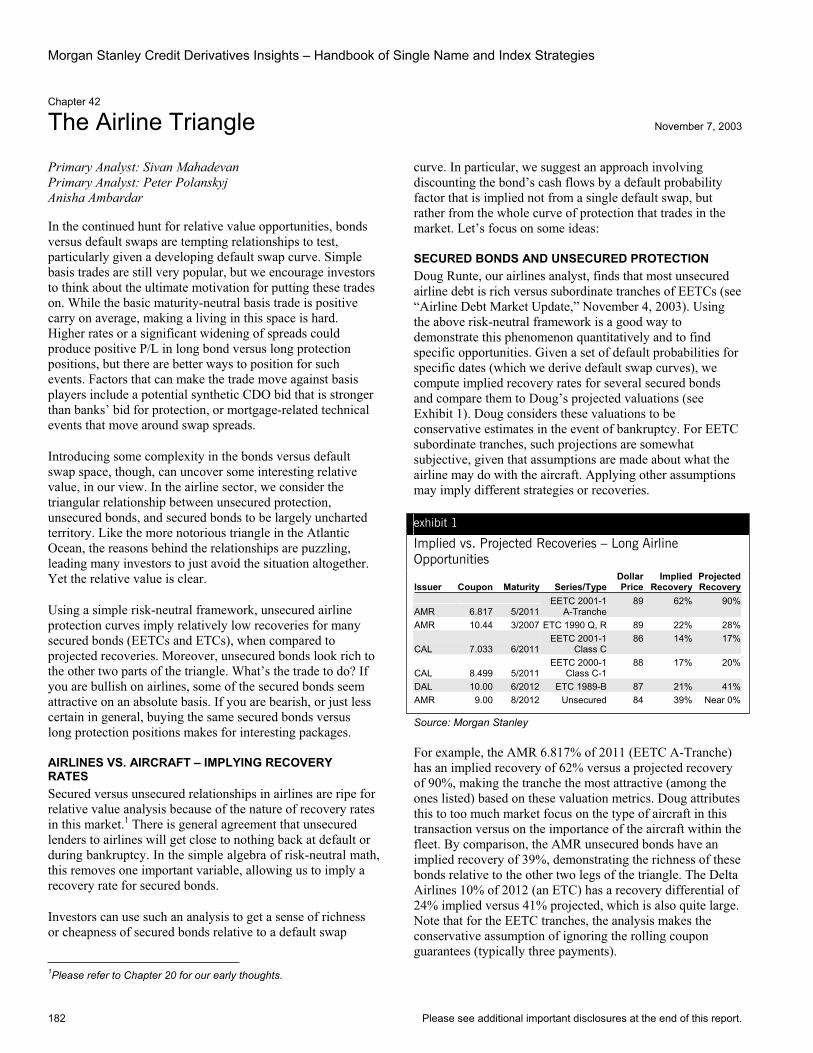
Morgan Stanley Credit Derivatives Insights – Handbook of Single Name and Index Strategies
182 Please see additional important disclosures at the end of this report.
Chapter 42
The Airline Triangle November 7, 2003
Primary Analyst: Sivan Mahadevan Primary Analyst: Peter Polanskyj Anisha Ambardar
In the continued hunt for relative value opportunities, bonds versus default swaps are tempting relationships to test, particularly given a developing default swap curve. Simple basis trades are still very popular, but we encourage investors to think about the ultimate motivation for putting these trades on. While the basic maturity-neutral basis trade is positive carry on average, making a living in this space is hard. Higher rates or a significant widening of spreads could produce positive P/L in long bond versus long protection positions, but there are better ways to position for such events. Factors that can make the trade move against basis players include a potential synthetic CDO bid that is stronger than banks’ bid for protection, or mortgage-related technical events that move around swap spreads.
Introducing some complexity in the bonds versus default swap space, though, can uncover some interesting relative value, in our view. In the airline sector, we consider the triangular relationship between unsecured protection, unsecured bonds, and secured bonds to be largely uncharted territory. Like the more notorious triangle in the Atlantic Ocean, the reasons behind the relationships are puzzling, leading many investors to just avoid the situation altogether. Yet the relative value is clear.
Using a simple risk-neutral framework, unsecured airline protection curves imply relatively low recoveries for many secured bonds (EETCs and ETCs), when compared to projected recoveries. Moreover, unsecured bonds look rich to the other two parts of the triangle. What’s the trade to do? If you are bullish on airlines, some of the secured bonds seem attractive on an absolute basis. If you are bearish, or just less certain in general, buying the same secured bonds versus long protection positions makes for interesting packages.
AIRLINES VS. AIRCRAFT – IMPLYING RECOVERY RATES Secured versus unsecured relationships in airlines are ripe for relative value analysis because of the nature of recovery rates in this market.1 There is general agreement that unsecured lenders to airlines will get close to nothing back at default or during bankruptcy. In the simple algebra of risk-neutral math, this removes one important variable, allowing us to imply a recovery rate for secured bonds.
Investors can use such an analysis to get a sense of richness or cheapness of secured bonds relative to a default swap
1Please refer to Chapter 20 for our early thoughts.
curve. In particular, we suggest an approach involving discounting the bond’s cash flows by a default probability factor that is implied not from a single default swap, but rather from the whole curve of protection that trades in the market. Let’s focus on some ideas:
SECURED BONDS AND UNSECURED PROTECTION Doug Runte, our airlines analyst, finds that most unsecured airline debt is rich versus subordinate tranches of EETCs (see “Airline Debt Market Update,” November 4, 2003). Using the above risk-neutral framework is a good way to demonstrate this phenomenon quantitatively and to find specific opportunities. Given a set of default probabilities for specific dates (which we derive default swap curves), we compute implied recovery rates for several secured bonds and compare them to Doug’s projected valuations (see Exhibit 1). Doug considers these valuations to be conservative estimates in the event of bankruptcy. For EETC subordinate tranches, such projections are somewhat subjective, given that assumptions are made about what the airline may do with the aircraft. Applying other assumptions may imply different strategies or recoveries.
exhibit 1
Implied vs. Projected Recoveries – Long Airline Opportunities
Issuer Coupon Maturity Series/Type Dollar Price
Implied Recovery
Projected Recovery
AMR 6.817 5/2011EETC 2001-1
A-Tranche89 62% 90%
AMR 10.44 3/2007 ETC 1990 Q, R 89 22% 28%
CAL 7.033 6/2011EETC 2001-1
Class C 86 14% 17%
CAL 8.499 5/2011EETC 2000-1
Class C-1 88 17% 20%
DAL 10.00 6/2012 ETC 1989-B 87 21% 41%AMR 9.00 8/2012 Unsecured 84 39% Near 0%
Source: Morgan Stanley
For example, the AMR 6.817% of 2011 (EETC A-Tranche) has an implied recovery of 62% versus a projected recovery of 90%, making the tranche the most attractive (among the ones listed) based on these valuation metrics. Doug attributes this to too much market focus on the type of aircraft in this transaction versus on the importance of the aircraft within the fleet. By comparison, the AMR unsecured bonds have an implied recovery of 39%, demonstrating the richness of these bonds relative to the other two legs of the triangle. The Delta Airlines 10% of 2012 (an ETC) has a recovery differential of 24% implied versus 41% projected, which is also quite large. Note that for the EETC tranches, the analysis makes the conservative assumption of ignoring the rolling coupon guarantees (typically three payments).
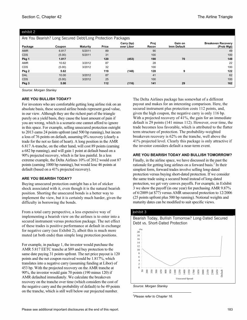
Section C, Chapter 42 The Airline Triangle
Please see additional important disclosures at the end of this report. 183
exhibit 2
Are You Bearish? Long Secured Debt/Long Protection Packages
Package Coupon Maturity PriceCarry (bp) over Libor
ProjRecov
Gain on Imm Default
Breakeven Recovery (Prob Wgt)
AMR 6.817 5/2011 89 90 49CDS (5.00) 5/2011 31 100 100Pkg 1 1.817 120 (453) 190 70 149AMR 10.62 3/2012 87 28 22CDS (5.00) 3/2012 32 100 100Pkg 2 5.62 119 (148) 128 9 122DAL 10.00 3/2012 87 41 62CDS (5.00) 3/2012 25 100 100Pkg 3 5.00 112 (116) 141 29 162
Source: Morgan Stanley
ARE YOU BULLISH TODAY? For investors who are comfortable getting long airline risk on an absolute basis, these secured airline bonds represent good value, in our view. Although they are the richest part of the triangle purely on a yield basis, they cause the least amount of pain if you are wrong, which is a scenario one cannot afford to ignore in this space. For example, selling unsecured protection outright to 2013 earns 24 points upfront (and 500 bp running), but incurs a loss of 76 points on default, assuming 0% recovery (clearly a trade for the not so faint of heart). A long position in the AMR 6.817 A-tranche, on the other hand, will cost 89 points (earning a 682 bp running), and will gain 1 point at default based on a 90% projected recovery, which is far less painful. In a less extreme example, the Delta Airlines 10% of 2012 would cost 87 points (earning 1000 bp running), but would lose 46 points at default (based on a 41% projected recovery).
ARE YOU BEARISH TODAY? Buying unsecured protection outright has a lot of sticker shock associated with it, even though it is the natural bearish position. Shorting the unsecured bonds is a better way to implement the view, but it is certainly much harder, given the difficulty in borrowing the bonds.
From a total carry perspective, a less expensive way of implementing a bearish view on the airlines is to enter into a secured instrument versus protection package. The net effect of these trades is positive performance at default in exchange for negative carry (see Exhibit 2), albeit this is much more muted (at both ends) than simple long protection positions.
For example, in package 1, the investor would purchase the AMR 5.817 EETC tranche at $89 and buy protection to the same date paying 31 points upfront. The net price payout is 120 points and the net coupon received would be 1.817%, which translates into a negative carry (assuming funding at Libor) of 453 bp. With the projected recovery on the AMR tranche at 90%, the investor would gain 70 points (190 minus 120) if AMR defaulted immediately. We calculate the breakeven recovery on the tranche over time (which considers the cost of the negative carry and the probability of default) to be 49 points on the tranche, which is still well below our projected number.
The Delta Airlines package has somewhat of a different payout and makes for an interesting comparison. Here, the secured instrument plus protection costs 112 points, and, given the high coupon, the negative carry is only 116 bp. With a projected recovery of 41%, the gain for an immediate default is 29 points (141 minus 112). However, over time, the trade becomes less favorable, which is attributed to the flatter term structure of protection. The probability-weighted breakeven recovery is 62% on the tranche, well above the 41% projected level. Clearly this package is only attractive if the investor considers default a near-term event.
ARE YOU BEARISH TODAY AND BULLISH TOMORROW? Finally, in the airline space, we have discussed in the past the rationale for getting long airlines on a forward basis.2 In their simplest form, forward trades involve selling long-dated protection versus buying short-dated protection. If we consider the same trade using a secured bond instead of long-dated protection, we get very convex payoffs. For example, in Exhibit 3 we show the payoff (in one year) for purchasing AMR 9.87% of 6/2009 (at $77) versus AMR unsecured protection to 12/2006 (25 points upfront plus 500 bp running). Notional weights and maturity dates can be modified to suit specific views.
exhibit 3
Bearish Today, Bullish Tomorrow? Long-Dated Secured Debt vs. Short-Dated Protection
(%)
02468
101214161820
50 200
350
500
650
800
950
1100
1250
1400
1550
1700
1850
2000
2150
2300
2450
Def
ault
Unsecured Spread
Source: Morgan Stanley
2Please refer to Chapter 16.

Morgan Stanley Credit Derivatives Insights – Handbook of Single Name and Index Strategies
184 Please see additional important disclosures at the end of this report.
Chapter 43
Oil Reshapes the Airline Triangle June 4, 2004
Primary Analyst: Sivan Mahadevan Primary Analyst: Peter Polanskyj Anisha Ambardar Angira Apte
One of the most fascinating cash versus default swap trading strategies exists in the airline space, where we have argued that the triangular relationship between unsecured protection and secured and unsecured debt instruments is an interesting, albeit sometimes treacherous, place to trade. When we last addressed this topic in detail, unsecured bonds seemed rich relative to CDS curves, while selected subordinated secured instruments appeared more attractive when comparing CDS implied recovery rates with projections from our airline team.1
Since that time, improving global economies have supported airline travel, boosting demand for aircraft and supporting values for secured debt. Yet, somewhat ironically, rising oil prices, poor oil hedging strategies and a lack of pricing power in the US industry have forced unsecured debt prices much lower. Furthermore, Delta Airline’s problems, which include a negative cashflow operating environment and a large number of retiring pilots (linked to pension incentives in a rising rate environment), are forcing the airline to flirt with bankruptcy. From a technical perspective, flows in Delta dominate liquidity, and the default swap markets have seen numerous new entrants from the equity hedge fund community recently. CDS curves for other airlines have moved wider in sympathy with Delta, although increased oil price is a real issue and is introducing “humps” in the curves, as well.
exhibit 1
Oil Spills into the Delta?
35
45
55
65
75
Jan-04 Feb-04 Mar-04 Apr-04 May-04 Jun-0432
34
36
38
40
42
44DAL 8.3 2029 (Left)
Crude Oil (WTI Spot) (Right)
Source: Morgan Stanley
1Please refer to Chapter 42.
The correlation breakdown (between secured and unsecured instruments) has interesting implications on the airline triangle. When we employ our implied recovery rate methodology, we find that unsecured bonds appear increasingly rich versus CDS curves, given current curve shapes and absolute moves in CDS premiums. Selected secured tranches seem more attractive, although most currently trade at levels that imply recovery rates above our analysts’ estimates.
THE AIRLINE TRIANGLE – THREE SIDES AND THREE THEMESThree themes seem to dominate day-to-day trading in the airline triangle. First, rising oil prices, coupled with improving economies, have caused an unexpected correlation breakdown between secured and unsecured legs. The scenario of significantly higher operating costs, coupled with stronger demand, was probably not a base case in most investors’ minds. Oil is now front-page news, with Middle East tensions and strong consumer demand (not to mention America’s love affair with SUVs) having a huge impact. The lack of pricing power in the industry is making the operational aspects of airlines riskier and is helping push unsecured bond prices lower (even away from Delta). For example, AMR Corp. and Northwest Airlines (NWAC) benchmark unsecured bonds are 10-20 points lower today, compared to first quarter 2004 levels. But improving travel, particularly in Europe and Asia, is supporting the EETC market by strengthening values of aircraft collateral. Many A-tranches still trade near par, and prices of select subordinate tranches are unchanged over the past several months.
Second, market activity late last year was dominated by only a handful of participants who could (or were willing) to trade the triangle. Today, there are plenty more players, most importantly in the equity hedge fund community, who are discovering that the term structure of unsecured airline protection offers interesting ways to implement long/short strategies with equity securities and options. Third, flows in Delta dominate liquidity, forcing a bit of a contagion impact on the other airlines, even if not fully justified.
WHAT ARE THE CURVES SAYING? Unsecured airline term structures (default swaps) have reshaped quite dramatically, given all of these market dynamics. Compared to late last year, equivalent running premiums are 200-300 bp wider, and the riskiest points in the curves have moved closer in, with the “hump” now consistently at a two-year point for AMR Corp. and Northwest Airlines (compared to three- and four-year points seven months ago). We argue that this reshaping is related to near-term operating risks in a higher oil price environment, as well as sympathy related to Delta Airlines.
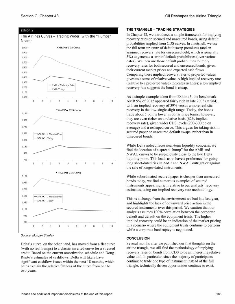
Section C, Chapter 43 Oil Reshapes the Airline Triangle
Please see additional important disclosures at the end of this report. 185
exhibit 2
The Airlines Curves – Trading Wider, with the “Humps” Nearer
AMR Par CDS Curve
1,000
1,100
1,200
1,300
1,400
1,500
1,600
1,700
1,800
1,900
2,000
1 2 3 4 5 6 7 8 9 10
AMR - 7 Months PriorAMR-Today
NWAC Par CDS Curve
750
950
1,150
1,350
1,550
1,750
1,950
2,150
1 2 3 4 5 6 7 8 9 10
NWAC - 7 Months Prior
NWAC - Today
NWAC Par CDS Curve
750
950
1,150
1,350
1,550
1,750
1,950
2,150
1 2 3 4 5 6 7 8 9 10
NWAC - 7 Months Prior
NWAC - Today
Source: Morgan Stanley
Delta’s curve, on the other hand, has moved from a flat curve (with no real humps) to a classic inverted curve for a stressed credit. Based on the current amortization schedule and Doug Runte’s estimates of cashflows, Delta will likely have significant cashflow issues within the next 18 months, which helps explain the relative flatness of the curve from one to two years.
THE TRIANGLE – TRADING STRATEGIES In Chapter 42, we introduced a simple framework for implying recovery rates on secured and unsecured bonds, using default probabilities implied from CDS curves. In a nutshell, we use the full term structure of default swap premiums (and an assumed recovery rate for unsecured debt, which is generally 5%) to generate a strip of default probabilities (over various dates). We then use those default probabilities to imply recovery rates for both secured and unsecured bonds, given their current market prices and expected cash flows. Comparing these implied recovery rates to projected values gives us a sense of relative value. A high implied recovery rate (relative to a projected value) indicates richness; a low implied recovery rate suggests the bond is cheap.
As a simple example taken from Exhibit 3, the benchmark AMR 9% of 2012 appeared fairly rich in late 2003 (at $84), with an implied recovery of 39% versus a more realistic recovery in the low-single-digit range. Today, the bonds trade about 5 points lower in dollar price terms; however, they are even richer on a relative basis (62% implied recovery rate), given wider CDS levels (200-300 bp on average) and a reshaped curve. This argues for taking risk in secured paper or unsecured default swaps, rather than in unsecured bonds.
While Delta indeed faces near-term liquidity concerns, we find the location of a spread “hump” for the AMR and NWAC curves to be suspiciously close to the key Delta liquidity point. This leads us to have a preference for going long short-dated risk in AMR and NWAC outright or against the sale of longer-dated instruments.
While subordinated secured paper is cheaper than unsecured bonds today, we find numerous examples of secured instruments appearing rich relative to our analysts’ recovery estimates, using our implied recovery rate methodology.
This is a change from the environment we had late last year, and highlights the lack of downward price action in the secured instruments over this period. We caution that our analysis assumes 100% correlation between the corporate default and default on the equipment trusts. The higher implied recovery could be an indication of the market pricing in a scenario where the equipment trusts continue to perform while a corporate bankruptcy is negotiated.
CONCLUSIONSeveral months after we published our first thoughts on the airline triangle, we still find the methodology of implying recovery rates on bonds from CDS to be an interesting relative value tool. In particular, since the majority of participants continue to trade one type of instrument instead of the full triangle, technically driven opportunities continue to exist.
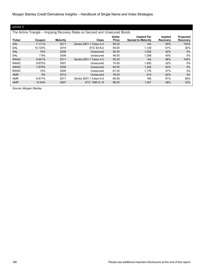
Morgan Stanley Credit Derivatives Insights – Handbook of Single Name and Index Strategies
186 Please see additional important disclosures at the end of this report.
exhibit 3
The Airline Triangle – Implying Recovery Rates on Secured and Unsecured Bonds
Ticker Coupon Maturity ClassDollarPrice
Implied Par Spread to Maturity
Implied Recovery
Projected Recovery
DAL 7.111% 2011 Series 2001-1 Class A-2 95.25 NA 90% 100%DAL 10.125% 2015 ETC 92 B-2 59.00 1,128 51% 30%DAL 10% 2008 Unsecured 50.00 1,638 42% 5%DAL 7.9% 2009 Unsecured 46.50 1,268 40% 5%NWAC 6.841% 2011 Series 2001-1 Class A-2 95.25 NA 88% 100%NWAC 9.875% 2007 Unsecured 74.00 1,492 32% 5%NWAC 7.875% 2008 Unsecured 65.00 1,292 40% 5%NWAC 10% 2009 Unsecured 67.25 1,176 47% 5%AMR 9% 2012 Unsecured 78.00 619 62% 5%AMR 6.817% 2011 Series 2001-1 Class A-2 90.00 NA 81% 95%AMR 10.44% 2007 ETC 1990 Q, R 88.00 1,447 48% 33%
Source: Morgan Stanley

Please see additional important disclosures at the end of this report. 187
Chapter 44
Turning a Triangle into a Square July 30, 2004
Primary Analyst: Sivan Mahadevan Primary Analyst: Peter Polanskyj Anisha Ambardar Angira Apte
Debt-versus-equity trading opportunities have been an area of market focus for some time now. “Capital structure arbitrage” was a popular “buzz” word at one point, but thankfully the market has gone beyond this nomenclature and focused more specifically on fundamental opportunities. In fact, if we had to characterize the state of debt-versus-equity trading today, we would say that it is indeed very opportunistic. For specific sectors or credits, relationships form because of linked market activity, but for the larger universe of companies, the relationship between the two markets is not necessarily as strong.
We find significant debt-versus-equity focus in the airline space, where investors in the credit and equity markets are eager to determine what investors in the other markets are saying and position ideas accordingly. In previous research, we discussed the rationale for and opportunities to trade what we called the airline triangle (comprised of secured bond, unsecured bond and unsecured default swap legs).1 The next leg of this trade is with equities, and many equity investors have discovered that default swap curves provide important market-implied probabilities of bankruptcy, which, in turn, can help determine relative value in equity or equity options. Similarly, many in the credit world can express views in the secured or unsecured airline space and hedge risks with equity securities. The triangle may be reshaping into a square.
One of the most difficult aspects of debt-versus-equity trades is determining what the right deltas should be, which is very much related to the current “regime” between the two instruments, and any expected convergence. We do not have any easy answers, nor are there market-standard approaches to solving these problems. A year ago, we used hindsight to calculate “best-fit” deltas, based on historical data, for a large universe of investment grade names (see “Puts vs. Protection – The Delta Divide,” July 25, 2003). We found that optimal deltas varied with spread and sector, as one might expect. What we find today is that most real activity in this space is in story credits, or, in the case of airlines, story sectors, so investors need to dig much deeper into company specific matters.
EQUITY AND CREDIT RELATIONSHIPS – GENERALLY SPEAKING One of the aspects of capital structure arbitrage that many find frustrating is deciding whether there are market triggers
1Please refer to Chapters 42 and 43.
to drive convergence. It is interesting to note that in today’s credit environment, the basic equity and credit relationships are actually rather weak, at least based on a reasonably broad and liquid segment of the market. In Exhibit 1, we show the average rolling 120-day correlation of credit spreads and equity prices for nearly 100 investment grade issuers. We show these both on an absolute and relative basis, where “relative” means that we subtract broader market movements from company specific spread and equity movements.
exhibit 1
Debt vs. Equity Not Necessarily Strongly Linked
Rolling Correlation
-0.7
-0.6
-0.5
-0.4
-0.3
-0.2
-0.1
0.0
0.1
0.2
Oct-01 Apr-02 Oct-02 Apr-03 Oct-03 Apr-04
Investment Grade Market (Relative)
Investment Grade Market (Absolute)
Source: Morgan Stanley
Clearly the 2002 time period was one where the relationships between equity and credit were stronger (more negative correlation), but since then, average correlation values have hovered in a tighter range, closer to zero. Currently the relative relationships are actually more stable than the absolute relationships, which we feel is noteworthy. This highlights the dangers that being outright long (or short) credit instruments against equities without hedging market risk has the potential to create unwanted volatility.
However, such market data does not provide a strong argument for capital structure arbitrage opportunities today. Nevertheless, we note two very important caveats. First, as we demonstrated in our aforementioned “Delta Divide” study, the link between equity options and credit spreads is generally stronger for lower-quality credits, by virtue of the more robust theoretical relationship between the two (i.e., both are driven by equity volatility, according to Merton models). Second, capital structure arbitrage is significantly different for story credits, precisely because market activity forces a stronger link, particularly in times of stress.
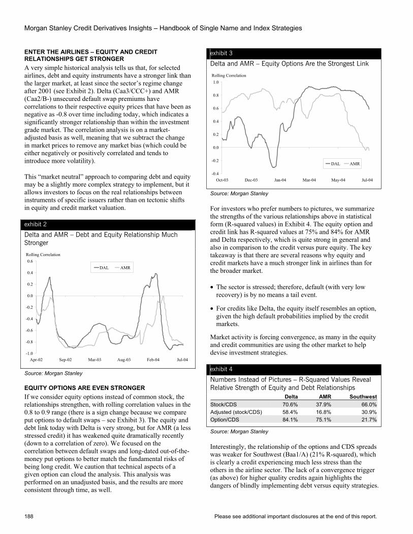
Morgan Stanley Credit Derivatives Insights – Handbook of Single Name and Index Strategies
188 Please see additional important disclosures at the end of this report.
ENTER THE AIRLINES – EQUITY AND CREDIT RELATIONSHIPS GET STRONGER A very simple historical analysis tells us that, for selected airlines, debt and equity instruments have a stronger link than the larger market, at least since the sector’s regime change after 2001 (see Exhibit 2). Delta (Caa3/CCC+) and AMR (Caa2/B-) unsecured default swap premiums have correlations to their respective equity prices that have been as negative as -0.8 over time including today, which indicates a significantly stronger relationship than within the investment grade market. The correlation analysis is on a market-adjusted basis as well, meaning that we subtract the change in market prices to remove any market bias (which could be either negatively or positively correlated and tends to introduce more volatility).
This “market neutral” approach to comparing debt and equity may be a slightly more complex strategy to implement, but it allows investors to focus on the real relationships between instruments of specific issuers rather than on tectonic shifts in equity and credit market valuation.
exhibit 2
Delta and AMR – Debt and Equity Relationship Much Stronger
Rolling Correlation
-1.0
-0.8
-0.6
-0.4
-0.2
0.0
0.2
0.4
0.6
Apr-02 Sep-02 Mar-03 Aug-03 Feb-04 Jul-04
DAL AMR
Source: Morgan Stanley
EQUITY OPTIONS ARE EVEN STRONGER If we consider equity options instead of common stock, the relationships strengthen, with rolling correlation values in the 0.8 to 0.9 range (there is a sign change because we compare put options to default swaps – see Exhibit 3). The equity and debt link today with Delta is very strong, but for AMR (a less stressed credit) it has weakened quite dramatically recently (down to a correlation of zero). We focused on the correlation between default swaps and long-dated out-of-the-money put options to better match the fundamental risks of being long credit. We caution that technical aspects of a given option can cloud the analysis. This analysis was performed on an unadjusted basis, and the results are more consistent through time, as well.
exhibit 3
Delta and AMR – Equity Options Are the Strongest Link
Rolling Correlation
-0.4
-0.2
0.0
0.2
0.4
0.6
0.8
1.0
Oct-03 Dec-03 Jan-04 Mar-04 May-04 Jul-04
DAL AMR
Source: Morgan Stanley
For investors who prefer numbers to pictures, we summarize the strengths of the various relationships above in statistical form (R-squared values) in Exhibit 4. The equity option and credit link has R-squared values at 75% and 84% for AMR and Delta respectively, which is quite strong in general and also in comparison to the credit versus pure equity. The key takeaway is that there are several reasons why equity and credit markets have a much stronger link in airlines than for the broader market.
• The sector is stressed; therefore, default (with very low recovery) is by no means a tail event.
• For credits like Delta, the equity itself resembles an option, given the high default probabilities implied by the credit markets.
Market activity is forcing convergence, as many in the equity and credit communities are using the other market to help devise investment strategies.
exhibit 4
Numbers Instead of Pictures – R-Squared Values Reveal Relative Strength of Equity and Debt Relationships Delta AMR SouthwestStock/CDS 70.6% 37.9% 66.0%Adjusted (stock/CDS) 58.4% 16.8% 30.9%Option/CDS 84.1% 75.1% 21.7%
Source: Morgan Stanley
Interestingly, the relationship of the options and CDS spreads was weaker for Southwest (Baa1/A) (21% R-squared), which is clearly a credit experiencing much less stress than the others in the airline sector. The lack of a convergence trigger (as above) for higher quality credits again highlights the dangers of blindly implementing debt versus equity strategies.
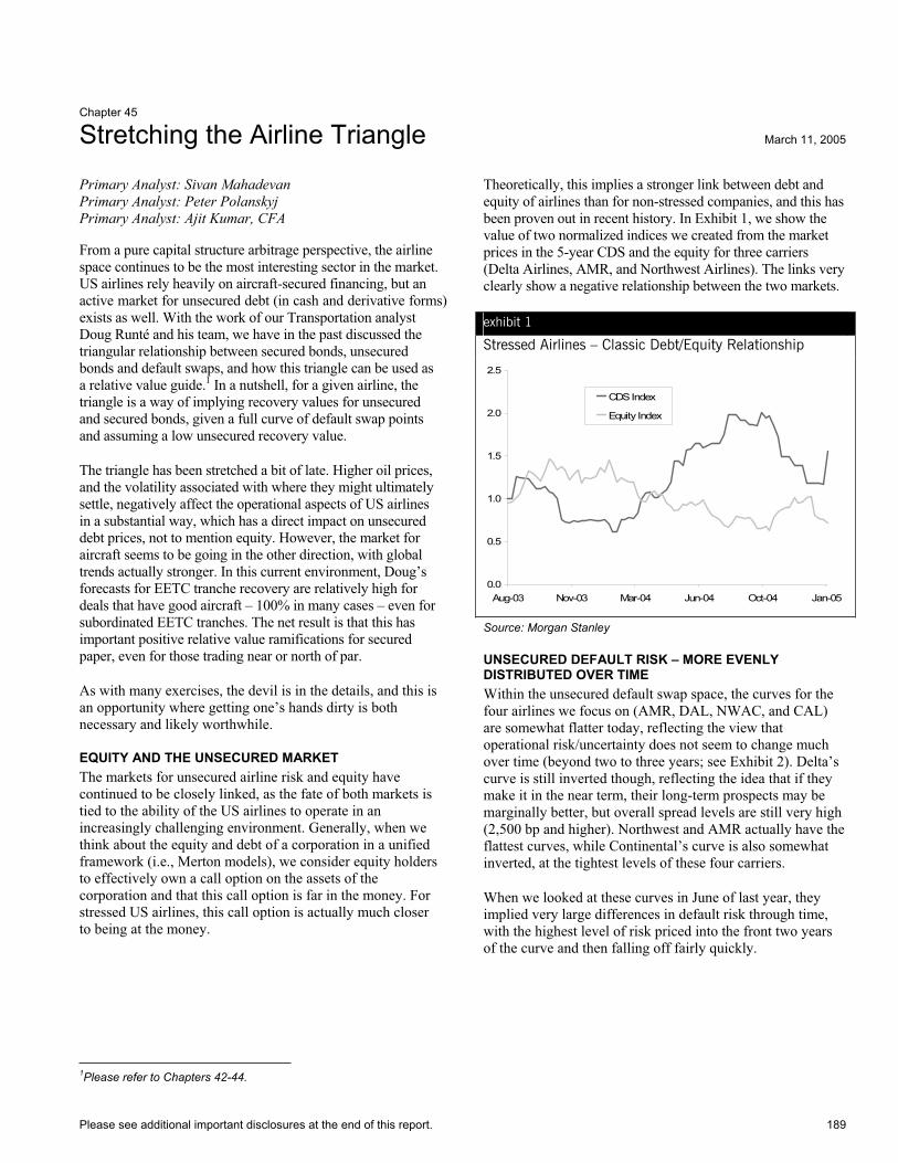
Please see additional important disclosures at the end of this report. 189
Chapter 45
Stretching the Airline Triangle March 11, 2005
Primary Analyst: Sivan Mahadevan Primary Analyst: Peter Polanskyj Primary Analyst: Ajit Kumar, CFA
From a pure capital structure arbitrage perspective, the airline space continues to be the most interesting sector in the market. US airlines rely heavily on aircraft-secured financing, but an active market for unsecured debt (in cash and derivative forms) exists as well. With the work of our Transportation analyst Doug Runté and his team, we have in the past discussed the triangular relationship between secured bonds, unsecured bonds and default swaps, and how this triangle can be used as a relative value guide.1 In a nutshell, for a given airline, the triangle is a way of implying recovery values for unsecured and secured bonds, given a full curve of default swap points and assuming a low unsecured recovery value.
The triangle has been stretched a bit of late. Higher oil prices, and the volatility associated with where they might ultimately settle, negatively affect the operational aspects of US airlines in a substantial way, which has a direct impact on unsecured debt prices, not to mention equity. However, the market for aircraft seems to be going in the other direction, with global trends actually stronger. In this current environment, Doug’s forecasts for EETC tranche recovery are relatively high for deals that have good aircraft – 100% in many cases – even for subordinated EETC tranches. The net result is that this has important positive relative value ramifications for secured paper, even for those trading near or north of par.
As with many exercises, the devil is in the details, and this is an opportunity where getting one’s hands dirty is both necessary and likely worthwhile.
EQUITY AND THE UNSECURED MARKET The markets for unsecured airline risk and equity have continued to be closely linked, as the fate of both markets is tied to the ability of the US airlines to operate in an increasingly challenging environment. Generally, when we think about the equity and debt of a corporation in a unified framework (i.e., Merton models), we consider equity holders to effectively own a call option on the assets of the corporation and that this call option is far in the money. For stressed US airlines, this call option is actually much closer to being at the money.
1Please refer to Chapters 42-44.
Theoretically, this implies a stronger link between debt and equity of airlines than for non-stressed companies, and this has been proven out in recent history. In Exhibit 1, we show the value of two normalized indices we created from the market prices in the 5-year CDS and the equity for three carriers (Delta Airlines, AMR, and Northwest Airlines). The links very clearly show a negative relationship between the two markets.
exhibit 1
Stressed Airlines – Classic Debt/Equity Relationship
0.0
0.5
1.0
1.5
2.0
2.5
Aug-03 Nov-03 Mar-04 Jun-04 Oct-04 Jan-05
CDS Index
Equity Index
Source: Morgan Stanley
UNSECURED DEFAULT RISK – MORE EVENLY DISTRIBUTED OVER TIME Within the unsecured default swap space, the curves for the four airlines we focus on (AMR, DAL, NWAC, and CAL) are somewhat flatter today, reflecting the view that operational risk/uncertainty does not seem to change much over time (beyond two to three years; see Exhibit 2). Delta’s curve is still inverted though, reflecting the idea that if they make it in the near term, their long-term prospects may be marginally better, but overall spread levels are still very high (2,500 bp and higher). Northwest and AMR actually have the flattest curves, while Continental’s curve is also somewhat inverted, at the tightest levels of these four carriers.
When we looked at these curves in June of last year, they implied very large differences in default risk through time, with the highest level of risk priced into the front two years of the curve and then falling off fairly quickly.

Morgan Stanley Credit Derivatives Insights – Handbook of Single Name and Index Strategies
190 Please see additional important disclosures at the end of this report.
exhibit 2a
DAL CDS Curve – Still Inverted, but Less So
bp
0
500
1,000
1,500
2,000
2,500
3,000
3,500
4,000
4,500
1 2 3 4 5 6 7 8 9 10Maturity
DAL 11/4/2003
DAL 6/4/2004
DAL 3/7/2005
Source: Morgan Stanley
exhibit 2b
AMR CDS Curve – Less Risky Early, Flat Later
bp
0
200
400
600
800
1,000
1,200
1,400
1,600
1,800
2,000
1 2 3 4 5 6 7 8 9 10Maturity
AMR 11/4/2003
AMR 6/4/2004
AMR 3/7/2005
Source: Morgan Stanley
exhibit 2c
NWAC CDS Curve – Turns Flat
bp
0
500
1,000
1,500
2,000
2,500
1 2 3 4 5 6 7 8 9 10Maturity
NWAC 11/4/2003
NWAC 6/4/2004
NWAC 3/7/2005
Source: Morgan Stanley
exhibit 2d
CAL CDS Curve – Slightly Inverted in Longer Dates
bp
0
500
1,000
1,500
2,000
2,500
1 2 3 4 5 6 7 8 9 10Maturity
CAL 11/4/2003
CAL 6/4/2004
CAL 3/7/2005
Source: Morgan Stanley
UNSECURED BONDS – THE NEXT LEG IN THE TRIANGLE With the unsecured default swap curves from above, we can now apply airline triangle methods to imply recoveries for unsecured bonds, which have a tendency to trade rich to default swaps, given appetite from investors and the difficulty in shorting bonds. The relative richness, though, seems to have fallen a bit since June of last year. In Exhibit 3, we show implied recoveries for one AMR unsecured bond, two Delta, bonds and two Northwest bonds. Assuming that actual recovery on unsecured debt is 5%, the AMR 9% of 2012 appears the richest of these five bonds, with a 42.5% implied recovery (versus implied recoveries of 13% to 21% for the others).
The most notable move (since last year) has been in DAL unsecured paper, which now trades to implied recoveries of 13% to 17% (for the two bonds highlighted).
SECURED PAPER – THE VERTEX OF THE TRIANGLE The market for aircraft continues to rally from global demand for aircraft. Doug recently pointed to strength both in the ATA bankruptcy proceedings and Geneva Aviation Forum (see “Aircraft Market Update,” February 28, 2005). For the numerous EETC tranches that we list in Exhibit 3, Doug estimates 100% recovery based on collateral valuations for many, including (in the case of AMR and Continental) some subtranches. Based on these estimates, EETC paper still seems relatively attractive, when recoveries are implied from the default swap curves, as valuations have only marginally improved in the face of a much stronger aircraft market. Senior tranches continue to trade at implied recoveries of approximately 80-90%, while the healthiest of subtranches have implied recoveries in the 50% to 60% range.

Section C, Chapter 45 Stretching the Airline Triangle
Please see additional important disclosures at the end of this report. 191
WHAT IS THE SECURED MARKET TELLING US? Our airline triangle approach uses risk-neutral models to imply the recoveries for secured bonds (note that we ignore the EETC liquidity facilities). As with most credit derivative models, we assume a fixed recovery over time. But the reality is somewhat different, and the volatility of valuations for aircraft since 2001 highlights this risk (which our models do not consider). As such, we would argue that there is a reasonable probability, based on historical movements, that aircraft valuations could fall at some point. EETC tranche investors need to be compensated for aircraft volatility above and beyond other risk premiums in the market for unsecured risk. This volatility is likely higher for subtranches than for senior tranches, and we remind market participants that there can be some “negotiation” risk for subtranche investors relative to senior tranche investors as well.
HOW CAN ONE MEASURE AND CAPTURE RELATIVE VALUE? In the past, many investors have asked us to take the airline triangle a step forward and determine how one can practically capture relative value, particularly with secured paper. In Exhibit 3 we go through a relatively simple process of calculating how an investor can go long secured paper and then hedge any residual risk, assuming Doug’s projected recoveries of the tranches. For example, the first tranche in the analysis (AMR A-1 tranche from series 99-1), trades at a price of 102.50%, leaving the investor with 2.5% of zero-recovery risk in the event of default (assuming 100% recovery based on aircraft). Clearly, any bond that is projected to have 100% recovery and trades wider than LIBOR has positive risk premium, and in this case, even after accounting for the 2.5% of default swap protection, the risk premium (or fully hedged bond spread) amounts to about 130 bp (last column of Exhibit 3). Furthermore, for bonds trading below par but expected to recover 100%, there is
over-collateralization that can be monetized (through the sale of default swap protection).
This hedged bond spread varies for different tranches, and is actually quite high for AMR, CAL, and even DAL subtranches (400 to 1,000 bp). Investors can view this metric as the carry for owning the secured paper relative to LIBOR and hedging any residual recovery risk with 5-year CDS.
WHAT ARE THE RISKS? What are the risks that one needs to be paid for? There are several, including the following:
• Aircraft recovery volatility
• Subtranche negotiation risk with senior tranches
• Unwind cost (bid-offer)
• Interest rate risk in the event of default (i.e., the asset swap would not be clean)
• Residual unsecured airline risk (we have used 5-year CDS as the hedging instrument for the sake of simplicity)
The hedged bond spread provides an indication of how much carry one can capture given today’s market prices. Whether or not these levels are attractive depends on how much one needs to be compensated for the risks above.
THE AIRLINE TRIANGLE We continue to find interesting relative value opportunities in the airline space, particularly when the challenging operational environment for many US airlines is juxtaposed against a more buoyant market for aircraft collateral. Yet, this is by no means an easy trade, as the secured debt side of the triangle requires quite a bit of analysis.
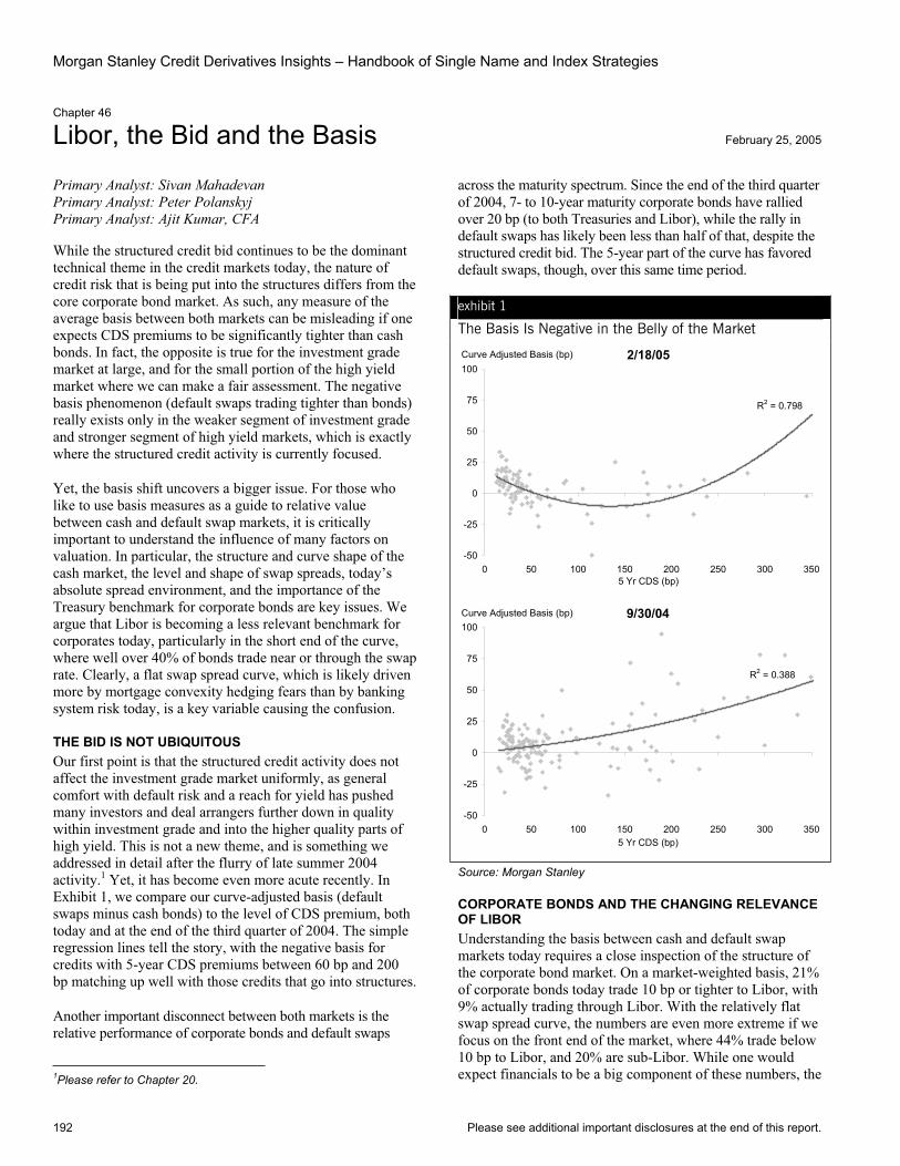
Morgan Stanley Credit Derivatives Insights – Handbook of Single Name and Index Strategies
192 Please see additional important disclosures at the end of this report.
Chapter 46
Libor, the Bid and the Basis February 25, 2005
Primary Analyst: Sivan Mahadevan Primary Analyst: Peter Polanskyj Primary Analyst: Ajit Kumar, CFA
While the structured credit bid continues to be the dominant technical theme in the credit markets today, the nature of credit risk that is being put into the structures differs from the core corporate bond market. As such, any measure of the average basis between both markets can be misleading if one expects CDS premiums to be significantly tighter than cash bonds. In fact, the opposite is true for the investment grade market at large, and for the small portion of the high yield market where we can make a fair assessment. The negative basis phenomenon (default swaps trading tighter than bonds) really exists only in the weaker segment of investment grade and stronger segment of high yield markets, which is exactly where the structured credit activity is currently focused.
Yet, the basis shift uncovers a bigger issue. For those who like to use basis measures as a guide to relative value between cash and default swap markets, it is critically important to understand the influence of many factors on valuation. In particular, the structure and curve shape of the cash market, the level and shape of swap spreads, today’s absolute spread environment, and the importance of the Treasury benchmark for corporate bonds are key issues. We argue that Libor is becoming a less relevant benchmark for corporates today, particularly in the short end of the curve, where well over 40% of bonds trade near or through the swap rate. Clearly, a flat swap spread curve, which is likely driven more by mortgage convexity hedging fears than by banking system risk today, is a key variable causing the confusion.
THE BID IS NOT UBIQUITOUS Our first point is that the structured credit activity does not affect the investment grade market uniformly, as general comfort with default risk and a reach for yield has pushed many investors and deal arrangers further down in quality within investment grade and into the higher quality parts of high yield. This is not a new theme, and is something we addressed in detail after the flurry of late summer 2004 activity.1 Yet, it has become even more acute recently. In Exhibit 1, we compare our curve-adjusted basis (default swaps minus cash bonds) to the level of CDS premium, both today and at the end of the third quarter of 2004. The simple regression lines tell the story, with the negative basis for credits with 5-year CDS premiums between 60 bp and 200 bp matching up well with those credits that go into structures.
Another important disconnect between both markets is the relative performance of corporate bonds and default swaps
1Please refer to Chapter 20.
across the maturity spectrum. Since the end of the third quarter of 2004, 7- to 10-year maturity corporate bonds have rallied over 20 bp (to both Treasuries and Libor), while the rally in default swaps has likely been less than half of that, despite the structured credit bid. The 5-year part of the curve has favored default swaps, though, over this same time period.
exhibit 1
The Basis Is Negative in the Belly of the Market
Curve Adjusted Basis (bp)
R2 = 0.798
-50
-25
0
25
50
75
100
0 50 100 150 200 250 300 3505 Yr CDS (bp)
2/18/05
Curve Adjusted Basis (bp)
R2 = 0.388
-50
-25
0
25
50
75
100
0 50 100 150 200 250 300 3505 Yr CDS (bp)
9/30/04
Source: Morgan Stanley
CORPORATE BONDS AND THE CHANGING RELEVANCE OF LIBOR Understanding the basis between cash and default swap markets today requires a close inspection of the structure of the corporate bond market. On a market-weighted basis, 21% of corporate bonds today trade 10 bp or tighter to Libor, with 9% actually trading through Libor. With the relatively flat swap spread curve, the numbers are even more extreme if we focus on the front end of the market, where 44% trade below 10 bp to Libor, and 20% are sub-Libor. While one would expect financials to be a big component of these numbers, the
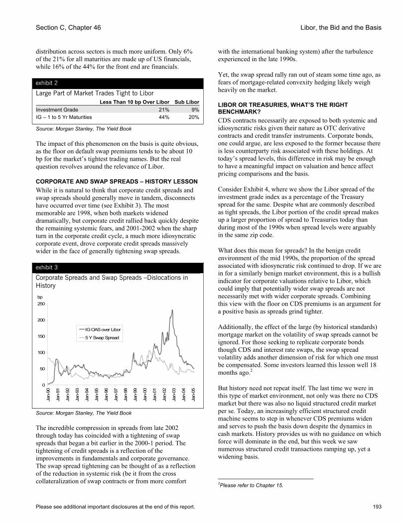
Section C, Chapter 46 Libor, the Bid and the Basis
Please see additional important disclosures at the end of this report. 193
distribution across sectors is much more uniform. Only 6% of the 21% for all maturities are made up of US financials, while 16% of the 44% for the front end are financials.
exhibit 2
Large Part of Market Trades Tight to Libor Less Than 10 bp Over Libor Sub LiborInvestment Grade 21% 9%IG – 1 to 5 Yr Maturities 44% 20%
Source: Morgan Stanley, The Yield Book
The impact of this phenomenon on the basis is quite obvious, as the floor on default swap premiums tends to be about 10 bp for the market’s tightest trading names. But the real question revolves around the relevance of Libor.
CORPORATE AND SWAP SPREADS – HISTORY LESSON While it is natural to think that corporate credit spreads and swap spreads should generally move in tandem, disconnects have occurred over time (see Exhibit 3). The most memorable are 1998, when both markets widened dramatically, but corporate credit rallied back quickly despite the remaining systemic fears, and 2001-2002 when the sharp turn in the corporate credit cycle, a much more idiosyncratic corporate event, drove corporate credit spreads massively wider in the face of generally tightening swap spreads.
exhibit 3
Corporate Spreads and Swap Spreads –Dislocations in History
0
50
100
150
200
250
Jan-
90
Jan-
91
Jan-
92
Jan-
93
Jan-
94
Jan-
95
Jan-
96
Jan-
97
Jan-
98
Jan-
99
Jan-
00
Jan-
01
Jan-
02
Jan-
03
Jan-
04
Jan-
05
bp
IG OAS over Libor
5 Y Swap Spread
Source: Morgan Stanley, The Yield Book
The incredible compression in spreads from late 2002 through today has coincided with a tightening of swap spreads that began a bit earlier in the 2000-1 period. The tightening of credit spreads is a reflection of the improvements in fundamentals and corporate governance. The swap spread tightening can be thought of as a reflection of the reduction in systemic risk (be it from the cross collateralization of swap contracts or from more comfort
with the international banking system) after the turbulence experienced in the late 1990s.
Yet, the swap spread rally ran out of steam some time ago, as fears of mortgage-related convexity hedging likely weigh heavily on the market.
LIBOR OR TREASURIES, WHAT’S THE RIGHT BENCHMARK? CDS contracts necessarily are exposed to both systemic and idiosyncratic risks given their nature as OTC derivative contracts and credit transfer instruments. Corporate bonds, one could argue, are less exposed to the former because there is less counterparty risk associated with these holdings. At today’s spread levels, this difference in risk may be enough to have a meaningful impact on valuation and hence affect pricing comparisons and the basis.
Consider Exhibit 4, where we show the Libor spread of the investment grade index as a percentage of the Treasury spread for the same. Despite what are commonly described as tight spreads, the Libor portion of the credit spread makes up a larger proportion of spread to Treasuries today than during most of the 1990s when spread levels were arguably in the same zip code.
What does this mean for spreads? In the benign credit environment of the mid 1990s, the proportion of the spread associated with idiosyncratic risk continued to drop. If we are in for a similarly benign market environment, this is a bullish indicator for corporate valuations relative to Libor, which could imply that potentially wider swap spreads are not necessarily met with wider corporate spreads. Combining this view with the floor on CDS premiums is an argument for a positive basis as spreads grind tighter.
Additionally, the effect of the large (by historical standards) mortgage market on the volatility of swap spreads cannot be ignored. For those seeking to replicate corporate bonds though CDS and interest rate swaps, the swap spread volatility adds another dimension of risk for which one must be compensated. Some investors learned this lesson well 18 months ago.2
But history need not repeat itself. The last time we were in this type of market environment, not only was there no CDS market but there was also no liquid structured credit market per se. Today, an increasingly efficient structured credit machine seems to step in whenever CDS premiums widen and serves to push the basis down despite the dynamics in cash markets. History provides us with no guidance on which force will dominate in the end, but this week we saw numerous structured credit transactions ramping up, yet a widening basis.
2Please refer to Chapter 15.

Morgan Stanley Credit Derivatives Insights – Handbook of Single Name and Index Strategies
194 Please see additional important disclosures at the end of this report.
We expect current basis themes to continue in the near term. For the lower-quality areas of the investment grade market, the basis will remain negative based on structured credit activity. For the market at large, swap spreads, however unrelated they may be to corporate credit risk, will likely be the key drivers of basis movements, as the battle between idiosyncratic and system risk continues.
exhibit 4
Corporates – Libor Spread as a % of Treasury Spread
0%
20%
40%
60%
80%
100%
120%
Jan-
90
Jan-
91
Jan-
92
Jan-
93
Jan-
94
Jan-
95
Jan-
96
Jan-
97
Jan-
98
Jan-
99
Jan-
00
Jan-
01
Jan-
02
Jan-
03
Jan-
04
Jan-
05
Source: Morgan Stanley
THE HIGH YIELD BASIS – SOME IMPROVEMENTS As an aside, despite an improving liquidity situation in high yield default swaps, calculating a fair value basis to bonds remains a challenging task for many reasons, including poor curve liquidity and the plethora of callable bonds. The good news is that we have improved our high yield basis monitor, which appears in our weekly Credit Derivatives Insights publication, to focus on credits where we have a good indication of valuation across the default swap curve and at
the five-year point of the bond market (non-callable). The bad news is that it leaves us with a relatively small universe (25 issuers).
Overall, the trends in the high yield basis remain intact and somewhat more pronounced in the updated universe. The basis remains positive (15 bp, 13 bp curve adjusted), with wider default swaps trading at a larger gap to the corresponding bonds. Difficulties in shorting high yield bonds, combined with a still developing single-name and structured credit market within high yield naturally force this basis to remain positive, especially with wider-trading names (see Exhibit 5). We continue to recommend that investors who have the flexibility of using both high yield bonds and default swaps consider using the positive basis as motivation for establishing long credit positions through default swaps.
exhibit 5
High Yield Basis – Largely Positive
R2 = 0.8605
-50
0
50
100
150
200
250
0 100 200 300 400 500 6005 yr CDS (bp)
Basis (bp)
Source: Morgan Stanley
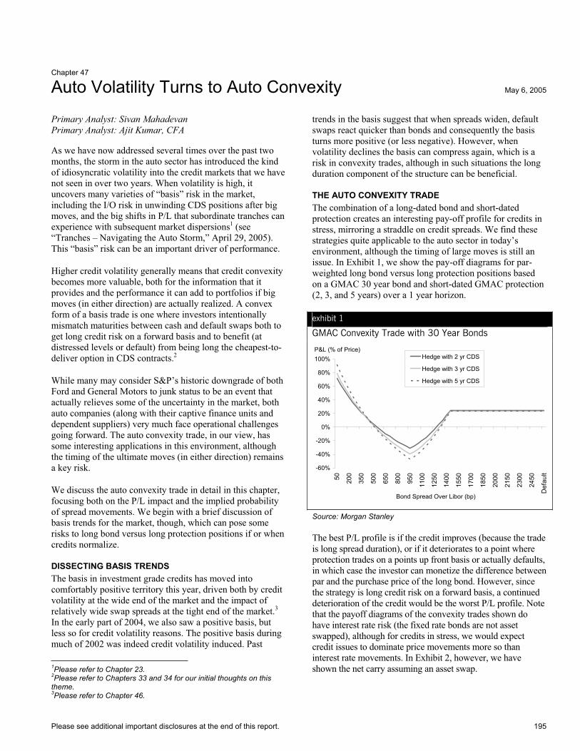
Please see additional important disclosures at the end of this report. 195
Chapter 47
Auto Volatility Turns to Auto Convexity May 6, 2005
Primary Analyst: Sivan Mahadevan Primary Analyst: Ajit Kumar, CFA
As we have now addressed several times over the past two months, the storm in the auto sector has introduced the kind of idiosyncratic volatility into the credit markets that we have not seen in over two years. When volatility is high, it uncovers many varieties of “basis” risk in the market, including the I/O risk in unwinding CDS positions after big moves, and the big shifts in P/L that subordinate tranches can experience with subsequent market dispersions1 (see “Tranches – Navigating the Auto Storm,” April 29, 2005). This “basis” risk can be an important driver of performance.
Higher credit volatility generally means that credit convexity becomes more valuable, both for the information that it provides and the performance it can add to portfolios if big moves (in either direction) are actually realized. A convex form of a basis trade is one where investors intentionally mismatch maturities between cash and default swaps both to get long credit risk on a forward basis and to benefit (at distressed levels or default) from being long the cheapest-to-deliver option in CDS contracts.2
While many may consider S&P’s historic downgrade of both Ford and General Motors to junk status to be an event that actually relieves some of the uncertainty in the market, both auto companies (along with their captive finance units and dependent suppliers) very much face operational challenges going forward. The auto convexity trade, in our view, has some interesting applications in this environment, although the timing of the ultimate moves (in either direction) remains a key risk.
We discuss the auto convexity trade in detail in this chapter, focusing both on the P/L impact and the implied probability of spread movements. We begin with a brief discussion of basis trends for the market, though, which can pose some risks to long bond versus long protection positions if or when credits normalize.
DISSECTING BASIS TRENDS The basis in investment grade credits has moved into comfortably positive territory this year, driven both by credit volatility at the wide end of the market and the impact of relatively wide swap spreads at the tight end of the market.3In the early part of 2004, we also saw a positive basis, but less so for credit volatility reasons. The positive basis during much of 2002 was indeed credit volatility induced. Past
1Please refer to Chapter 23. 2Please refer to Chapters 33 and 34 for our initial thoughts on this theme.3Please refer to Chapter 46.
trends in the basis suggest that when spreads widen, default swaps react quicker than bonds and consequently the basis turns more positive (or less negative). However, when volatility declines the basis can compress again, which is a risk in convexity trades, although in such situations the long duration component of the structure can be beneficial.
THE AUTO CONVEXITY TRADE The combination of a long-dated bond and short-dated protection creates an interesting pay-off profile for credits in stress, mirroring a straddle on credit spreads. We find these strategies quite applicable to the auto sector in today’s environment, although the timing of large moves is still an issue. In Exhibit 1, we show the pay-off diagrams for par-weighted long bond versus long protection positions based on a GMAC 30 year bond and short-dated GMAC protection (2, 3, and 5 years) over a 1 year horizon.
exhibit 1
GMAC Convexity Trade with 30 Year Bonds
P&L (% of Price)
-60%
-40%
-20%
0%
20%
40%
60%
80%
100%
50 200
350
500
650
800
950
1100
1250
1400
1550
1700
1850
2000
2150
2300
2450
Def
ault
Bond Spread Over Libor (bp)
Hedge with 2 yr CDS
Hedge with 3 yr CDS
Hedge with 5 yr CDS
Source: Morgan Stanley
The best P/L profile is if the credit improves (because the trade is long spread duration), or if it deteriorates to a point where protection trades on a points up front basis or actually defaults, in which case the investor can monetize the difference between par and the purchase price of the long bond. However, since the strategy is long credit risk on a forward basis, a continued deterioration of the credit would be the worst P/L profile. Note that the payoff diagrams of the convexity trades shown do have interest rate risk (the fixed rate bonds are not asset swapped), although for credits in stress, we would expect credit issues to dominate price movements more so than interest rate movements. In Exhibit 2, however, we have shown the net carry assuming an asset swap.
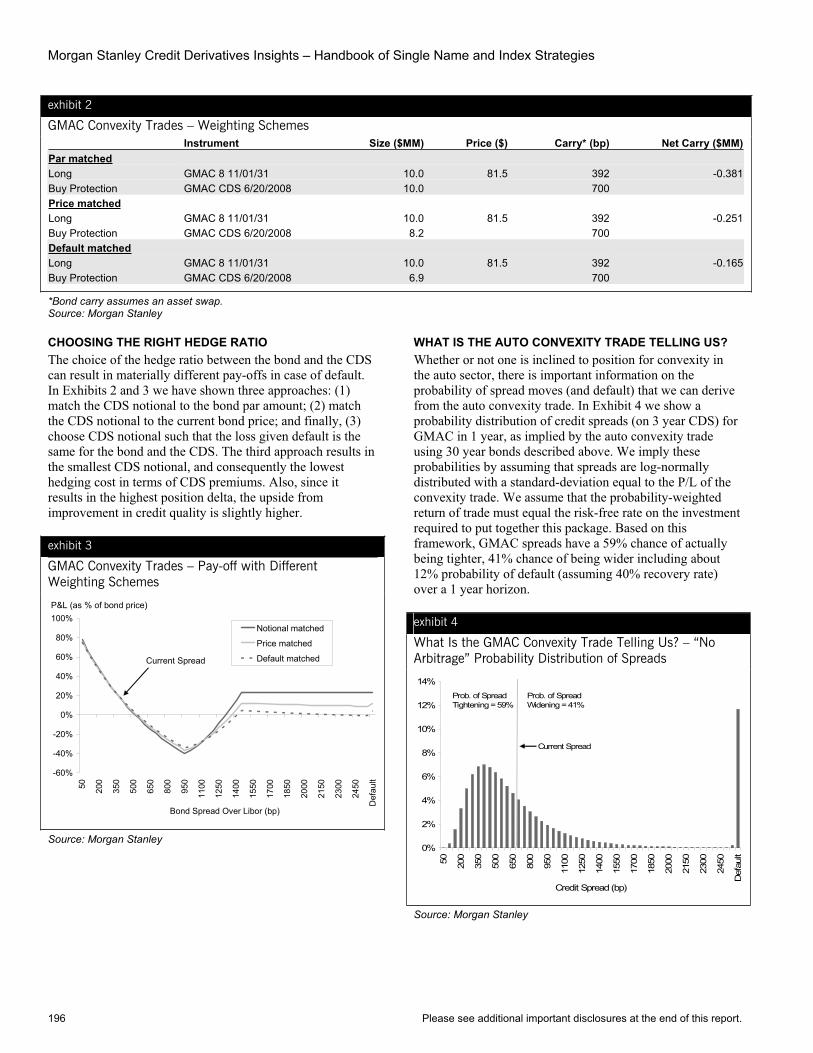
Morgan Stanley Credit Derivatives Insights – Handbook of Single Name and Index Strategies
196 Please see additional important disclosures at the end of this report.
exhibit 2
GMAC Convexity Trades – Weighting Schemes Instrument Size ($MM) Price ($) Carry* (bp) Net Carry ($MM)Par matchedLong GMAC 8 11/01/31 10.0 81.5 392 -0.381Buy Protection GMAC CDS 6/20/2008 10.0 700Price matchedLong GMAC 8 11/01/31 10.0 81.5 392 -0.251Buy Protection GMAC CDS 6/20/2008 8.2 700 Default matchedLong GMAC 8 11/01/31 10.0 81.5 392 -0.165Buy Protection GMAC CDS 6/20/2008 6.9 700
*Bond carry assumes an asset swap. Source: Morgan Stanley
CHOOSING THE RIGHT HEDGE RATIO The choice of the hedge ratio between the bond and the CDS can result in materially different pay-offs in case of default. In Exhibits 2 and 3 we have shown three approaches: (1) match the CDS notional to the bond par amount; (2) match the CDS notional to the current bond price; and finally, (3) choose CDS notional such that the loss given default is the same for the bond and the CDS. The third approach results in the smallest CDS notional, and consequently the lowest hedging cost in terms of CDS premiums. Also, since it results in the highest position delta, the upside from improvement in credit quality is slightly higher.
exhibit 3
GMAC Convexity Trades – Pay-off with Different Weighting Schemes
P&L (as % of bond price)
-60%
-40%
-20%
0%
20%
40%
60%
80%
100%
50 200
350
500
650
800
950
1100
1250
1400
1550
1700
1850
2000
2150
2300
2450
Def
ault
Bond Spread Over Libor (bp)
Notional matched
Price matched
Default matchedCurrent Spread
Source: Morgan Stanley
WHAT IS THE AUTO CONVEXITY TRADE TELLING US? Whether or not one is inclined to position for convexity in the auto sector, there is important information on the probability of spread moves (and default) that we can derive from the auto convexity trade. In Exhibit 4 we show a probability distribution of credit spreads (on 3 year CDS) for GMAC in 1 year, as implied by the auto convexity trade using 30 year bonds described above. We imply these probabilities by assuming that spreads are log-normally distributed with a standard-deviation equal to the P/L of the convexity trade. We assume that the probability-weighted return of trade must equal the risk-free rate on the investment required to put together this package. Based on this framework, GMAC spreads have a 59% chance of actually being tighter, 41% chance of being wider including about 12% probability of default (assuming 40% recovery rate) over a 1 year horizon.
exhibit 4
What Is the GMAC Convexity Trade Telling Us? – “No Arbitrage” Probability Distribution of Spreads
0%
2%
4%
6%
8%
10%
12%
14%
50 200
350
500
650
800
950
1100
1250
1400
1550
1700
1850
2000
2150
2300
2450
Def
ault
Credit Spread (bp)
Prob. of SpreadWidening = 41%
Prob. of SpreadTightening = 59%
Current Spread
Source: Morgan Stanley
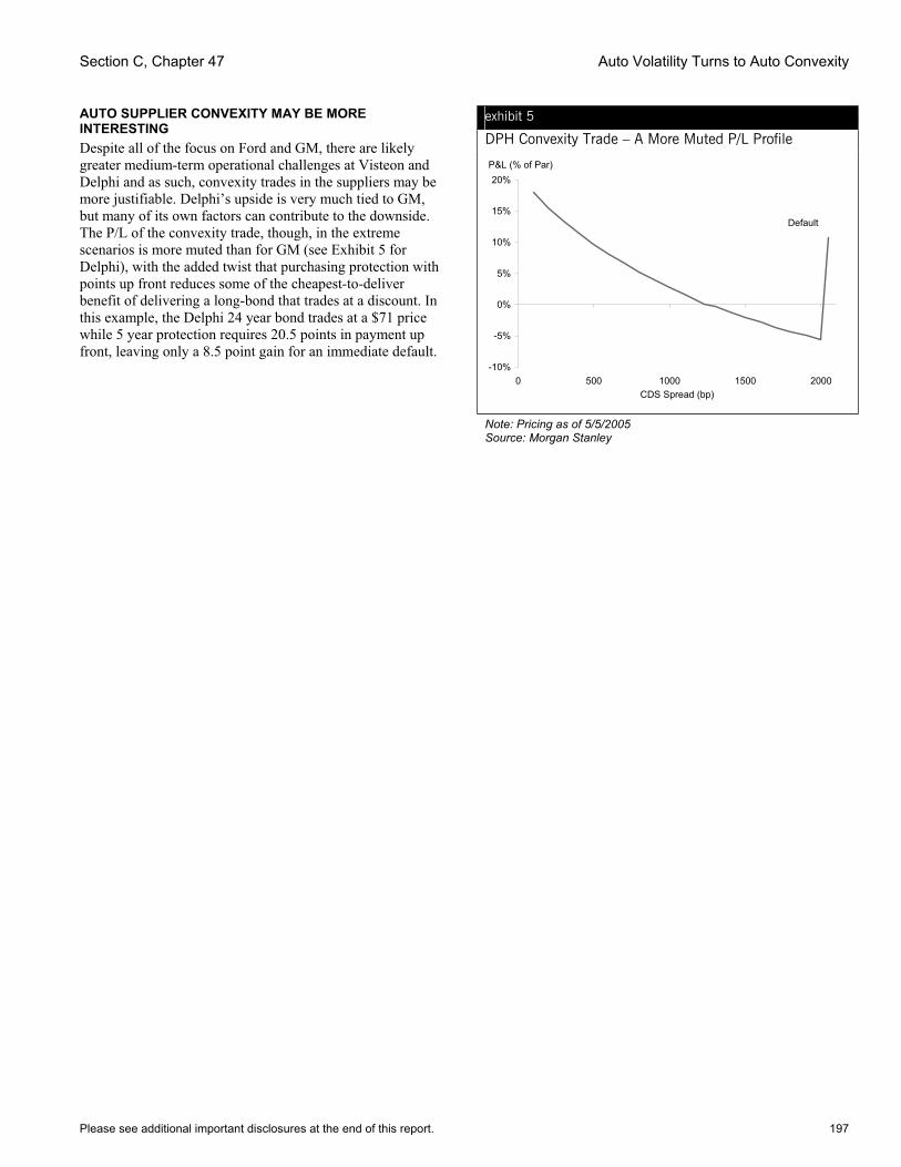
Section C, Chapter 47 Auto Volatility Turns to Auto Convexity
Please see additional important disclosures at the end of this report. 197
AUTO SUPPLIER CONVEXITY MAY BE MORE INTERESTING Despite all of the focus on Ford and GM, there are likely greater medium-term operational challenges at Visteon and Delphi and as such, convexity trades in the suppliers may be more justifiable. Delphi’s upside is very much tied to GM, but many of its own factors can contribute to the downside. The P/L of the convexity trade, though, in the extreme scenarios is more muted than for GM (see Exhibit 5 for Delphi), with the added twist that purchasing protection with points up front reduces some of the cheapest-to-deliver benefit of delivering a long-bond that trades at a discount. In this example, the Delphi 24 year bond trades at a $71 price while 5 year protection requires 20.5 points in payment up front, leaving only a 8.5 point gain for an immediate default.
exhibit 5
DPH Convexity Trade – A More Muted P/L Profile
P&L (% of Par)
-10%
-5%
0%
5%
10%
15%
20%
0 500 1000 1500 2000CDS Spread (bp)
Default
Note: Pricing as of 5/5/2005 Source: Morgan Stanley

Morgan Stanley Credit Derivatives Insights – Handbook of Single Name and Index Strategies
198 Please see additional important disclosures at the end of this report.
Chapter 48
Playing LBOs with CDS – Details, Details… October 7, 2005
Primary Analyst: Sivan Mahadevan Primary Analyst: Peter Polanskyj
Several forces in the market today have been responsible for introducing significant capital structure changes into both investment grade and high yield companies, including a ripe LBO environment and the related existence of cash-rich potential sponsors from the hedge fund and private equity worlds. In many such cases, understanding the potential performance of bonds and default swaps has been at a minimum an insightful exercise in credit fundamentals, but more importantly it highlights the differing “basis” risks that can come to the forefront, particularly when the use of bond and loan covenants (or lack thereof) influences capital structure shifts.
As such, critically important in the process of understanding the credit pricing dynamics during recapitalizations are the details in the indentures of all the bonds involved and the likely financing strategy of an acquirer. Whether bonds would be tendered or remain outstanding is a key driver in their valuations going into recapitalizations, and CDS contracts serve as generic instruments which could continue to be exposed to the credit risk regardless of the fate of the existing company debt.
In this chapter, we go through three real-world examples of bond versus default swap performance during capital structure shifts to illustrate some of the “basis” risks between the instruments, and we provide some covenant background as well.
CDS AS THE LEAST COMMON DENOMINATOR The key to trading bonds versus CDS contracts in the context of recapitalizations really comes down to the specific covenants in a particular bond issue and how that covenant package affects the risk in that issue as compared to both the other existing bonds in the capital structure and any bonds/loans likely to be issued as part of a new recapitalization plan.
The fact that we must consider newly issued instruments in the context of recapitalizations is a result of the cheapest-to-deliver options associated with CDS contracts. Any existing CDS contracts are generally not retired when old debt is tendered for or is repurchased, therefore they remain outstanding. In recapitalizations, that means they will be anchored, at least in price terms, to the riskiest senior instruments of the entity (assuming the original CDS is a typical senior unsecured contract). This fact is often stated as part of the argument for a positive basis between CDS and bonds of the same maturity, when capital structure changes are a possibility.
TYPICAL BOND COVENANTS While, anecdotally, we know that most US investment grade transactions have few covenants, we can look to the high yield market to illustrate what covenants can be required by investors. Having a sense for the form of typical covenants can provide some insight as to their potential impact on the performance of the bonds in recapitalizations.
The following is a list of some common covenants included in high yield issues:
Limitation on Restricted Payments: Effectively restricts dividend payments, purchases of equity or subordinated debt of the issuing entity or subsidiaries to some proportion of net income, cashflow or an absolute dollar amount.
Limitation on Incurrence of Indebtedness: Generally limits the ability of the issuer to incur additional indebtedness subject to financial ratios, commonly, the ratio of consolidated cash flow to fixed charges.
Limitation on Asset Sales: Constrains the sale, lease, conveyance or other disposition of assets or equity held in subsidiaries (other than inventory) without offering to repurchase notes.
Payment Restrictions Affecting Subsidiaries: Restricts the ability of the issuer to create an encumbrance or restriction on the ability of subsidiaries to pay dividends to the issuer.
Limitation on Merger, Consolidation, or Sale of Assets: Limits the ability of the entity or subsidiary guarantors to merge under certain circumstances.
Limitation on Affiliate Transactions: Constrains the ability of the issuer to sell, lease, transfer or otherwise dispose of any assets to an affiliate.
Limitation on Liens: Constrains the ability of the issuer to cause any new liens unless all payments due on existing debt are secured on an equal and ratable basis with obligations so secured.
Limitation on Sale/Leaseback Transactions: Restricts the ability of sale/leaseback transactions.
Of these covenants, the limitation on liens has been the most visible recently, given the reliance of LBOs on the leveraged loan market which is generally a secured market. This covenant comes into play in very different ways in our examples below.
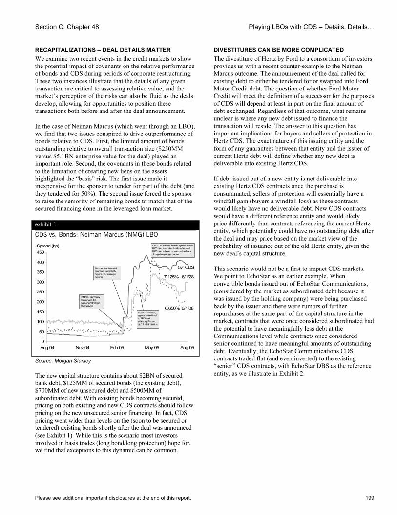
Section C, Chapter 48 Playing LBOs with CDS – Details, Details…
Please see additional important disclosures at the end of this report. 199
RECAPITALIZATIONS – DEAL DETAILS MATTER We examine two recent events in the credit markets to show the potential impact of covenants on the relative performance of bonds and CDS during periods of corporate restructuring. These two instances illustrate that the details of any given transaction are critical to assessing relative value, and the market’s perception of the risks can also be fluid as the deals develop, allowing for opportunities to position these transactions both before and after the deal announcement.
In the case of Neiman Marcus (which went through an LBO), we find that two issues conspired to drive outperformance of bonds relative to CDS. First, the limited amount of bonds outstanding relative to overall transaction size ($250MM versus $5.1BN enterprise value for the deal) played an important role. Second, the covenants in these bonds related to the limitation of creating new liens on the assets highlighted the “basis” risk. The first issue made it inexpensive for the sponsor to tender for part of the debt (and they tendered for 50%). The second issue forced the sponsor to raise the seniority of remaining bonds to match that of the secured financing done in the leveraged loan market.
exhibit 1
CDS vs. Bonds: Neiman Marcus (NMG) LBO
Spread (bp)
5yr CDS
6.650% 6/1/08
7.125% 6/1/28
0
50
100
150
200
250
300
350
400
450
Aug-04 Nov-04 Feb-05 May-05 Aug-05
5 Yr CDS flattens, Bonds tighten as the 2008 bonds receive tender offer and 2028 bonds become secured on back of negative pledge clause
5/2/05- Company agrees to sell itself to TPG and Warburg Pincus LLC for $5.1 billion
Rumors that financial sponsors were likely buyers (vs. strategic buyers)
3/14/05- Company announces it is pursuing “strategic alternatives”
Source: Morgan Stanley
The new capital structure contains about $2BN of secured bank debt, $125MM of secured bonds (the existing debt), $700MM of new unsecured debt and $500MM of subordinated debt. With existing bonds becoming secured, pricing on both existing and new CDS contracts should follow pricing on the new unsecured senior financing. In fact, CDS pricing went wider than levels on the (soon to be secured or tendered) existing bonds shortly after the deal was announced (see Exhibit 1). While this is the scenario most investors involved in basis trades (long bond/long protection) hope for, we find that exceptions to this dynamic can be common.
DIVESTITURES CAN BE MORE COMPLICATED The divestiture of Hertz by Ford to a consortium of investors provides us with a recent counter-example to the Neiman Marcus outcome. The announcement of the deal called for existing debt to either be tendered for or swapped into Ford Motor Credit debt. The question of whether Ford Motor Credit will meet the definition of a successor for the purposes of CDS will depend at least in part on the final amount of debt exchanged. Regardless of that outcome, what remains unclear is where any new debt issued to finance the transaction will reside. The answer to this question has important implications for buyers and sellers of protection in Hertz CDS. The exact nature of this issuing entity and the form of any guarantees between that entity and the issuer of current Hertz debt will define whether any new debt is deliverable into existing Hertz CDS.
If debt issued out of a new entity is not deliverable into existing Hertz CDS contracts once the purchase is consummated, sellers of protection will essentially have a windfall gain (buyers a windfall loss) as these contracts would likely have no deliverable debt. New CDS contracts would have a different reference entity and would likely price differently than contracts referencing the current Hertz entity, which potentially could have no outstanding debt after the deal and may price based on the market view of the probability of issuance out of the old Hertz entity, given the new deal’s capital structure.
This scenario would not be a first to impact CDS markets. We point to EchoStar as an earlier example. When convertible bonds issued out of EchoStar Communications, (considered by the market as subordinated debt because it was issued by the holding company) were being purchased back by the issuer and there were rumors of further repurchases at the same part of the capital structure in the market, contracts that were once considered subordinated had the potential to have meaningfully less debt at the Communications level while contracts once considered senior continued to have meaningful amounts of outstanding debt. Eventually, the EchoStar Communications CDS contracts traded flat (and even inverted) to the existing “senior” CDS contracts, with EchoStar DBS as the reference entity, as we illustrate in Exhibit 2.
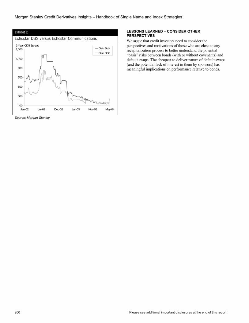
Morgan Stanley Credit Derivatives Insights – Handbook of Single Name and Index Strategies
200 Please see additional important disclosures at the end of this report.
exhibit 2
Echostar DBS versus Echostar Communications
5 Year CDS Spread
100
300
500
700
900
1,100
1,300
Jan-02 Jul-02 Dec-02 Jun-03 Nov-03 May-04
Dish Sub
Dish DBS
Source: Morgan Stanley
LESSONS LEARNED – CONSIDER OTHER PERSPECTIVESWe argue that credit investors need to consider the perspectives and motivations of those who are close to any recapitalization process to better understand the potential “basis” risks between bonds (with or without covenants) and default swaps. The cheapest to deliver nature of default swaps (and the potential lack of interest in them by sponsors) has meaningful implications on performance relative to bonds.
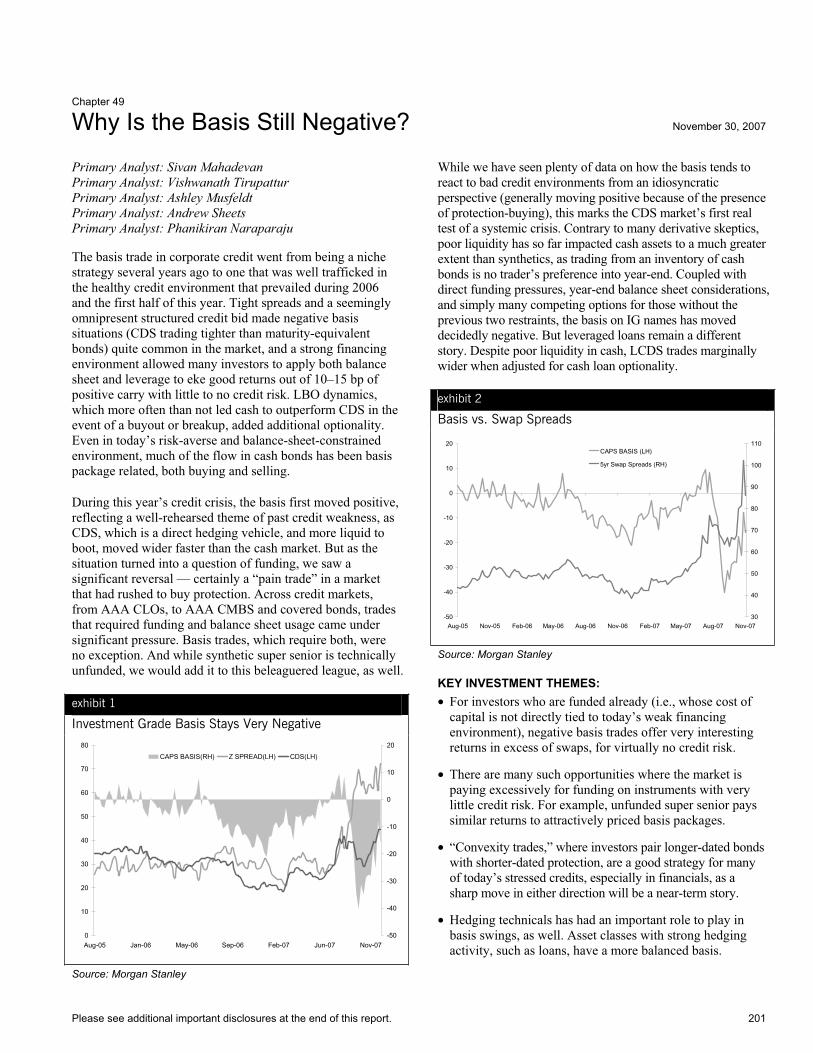
Please see additional important disclosures at the end of this report. 201
Chapter 49
Why Is the Basis Still Negative? November 30, 2007
Primary Analyst: Sivan Mahadevan Primary Analyst: Vishwanath Tirupattur Primary Analyst: Ashley Musfeldt Primary Analyst: Andrew Sheets Primary Analyst: Phanikiran Naraparaju
The basis trade in corporate credit went from being a niche strategy several years ago to one that was well trafficked in the healthy credit environment that prevailed during 2006 and the first half of this year. Tight spreads and a seemingly omnipresent structured credit bid made negative basis situations (CDS trading tighter than maturity-equivalent bonds) quite common in the market, and a strong financing environment allowed many investors to apply both balance sheet and leverage to eke good returns out of 10–15 bp of positive carry with little to no credit risk. LBO dynamics, which more often than not led cash to outperform CDS in the event of a buyout or breakup, added additional optionality. Even in today’s risk-averse and balance-sheet-constrained environment, much of the flow in cash bonds has been basis package related, both buying and selling.
During this year’s credit crisis, the basis first moved positive, reflecting a well-rehearsed theme of past credit weakness, as CDS, which is a direct hedging vehicle, and more liquid to boot, moved wider faster than the cash market. But as the situation turned into a question of funding, we saw a significant reversal — certainly a “pain trade” in a market that had rushed to buy protection. Across credit markets, from AAA CLOs, to AAA CMBS and covered bonds, trades that required funding and balance sheet usage came under significant pressure. Basis trades, which require both, were no exception. And while synthetic super senior is technically unfunded, we would add it to this beleaguered league, as well.
exhibit 1
Investment Grade Basis Stays Very Negative
0
10
20
30
40
50
60
70
80
Aug-05 Jan-06 May-06 Sep-06 Feb-07 Jun-07 Nov-07-50
-40
-30
-20
-10
0
10
20
CAPS BASIS(RH) Z SPREAD(LH) CDS(LH)
Source: Morgan Stanley
While we have seen plenty of data on how the basis tends to react to bad credit environments from an idiosyncratic perspective (generally moving positive because of the presence of protection-buying), this marks the CDS market’s first real test of a systemic crisis. Contrary to many derivative skeptics, poor liquidity has so far impacted cash assets to a much greater extent than synthetics, as trading from an inventory of cash bonds is no trader’s preference into year-end. Coupled with direct funding pressures, year-end balance sheet considerations, and simply many competing options for those without the previous two restraints, the basis on IG names has moved decidedly negative. But leveraged loans remain a different story. Despite poor liquidity in cash, LCDS trades marginally wider when adjusted for cash loan optionality.
exhibit 2
Basis vs. Swap Spreads
-50
-40
-30
-20
-10
0
10
20
Aug-05 Nov-05 Feb-06 May-06 Aug-06 Nov-06 Feb-07 May-07 Aug-07 Nov-0730
40
50
60
70
80
90
100
110CAPS BASIS (LH)
5yr Swap Spreads (RH)
Source: Morgan Stanley
KEY INVESTMENT THEMES: • For investors who are funded already (i.e., whose cost of
capital is not directly tied to today’s weak financing environment), negative basis trades offer very interesting returns in excess of swaps, for virtually no credit risk.
• There are many such opportunities where the market is paying excessively for funding on instruments with very little credit risk. For example, unfunded super senior pays similar returns to attractively priced basis packages.
• “Convexity trades,” where investors pair longer-dated bonds with shorter-dated protection, are a good strategy for many of today’s stressed credits, especially in financials, as a sharp move in either direction will be a near-term story.
• Hedging technicals has had an important role to play in basis swings, as well. Asset classes with strong hedging activity, such as loans, have a more balanced basis.
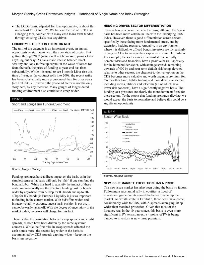
Morgan Stanley Credit Derivatives Insights – Handbook of Single Name and Index Strategies
202 Please see additional important disclosures at the end of this report.
• The LCDS basis, adjusted for loan optionality, is about flat, in contrast to IG and HY. We believe the use of LCDX as a hedging tool, coupled with many cash loans term funded through existing CLOs, is a key driver.
LIQUIDITY: EITHER IT IS THERE OR NOT The turn of the calendar is an important event, an annual opportunity to start anew with the allocation of capital. But getting through 2007 (which will not be missed) proves to be anything but easy. As banks face intense balance sheet scrutiny and look to free up capital in the wake of losses (or fears thereof), the price of funding to year-end has risen substantially. While it is usual to see 1-month Libor rise this time of year, as the contract rolls into 2008, the recent spike has been substantially more pronounced than for prior years (see Exhibit 3). However, the year-end factor is not the only story here, by any measure. Many gauges of longer-dated funding environment also continue to creep wider.
exhibit 3
Short and Long-Term Funding Sentiment
1M Libor - 1M T-Bill (bp)
0
20
40
60
80
100
120
140
160
180
200
-100102030405060Trading Days to New Year
2003 2004 2005 2006 2007
Source: Morgan Stanley
Funding pressures have a direct impact on the basis, as in the simplest sense a flat basis will only be “fair” if one can fund the bond at Libor. While it is hard to quantify the impact of these costs, we anecdotally see the effective funding cost for bonds wider by anywhere from 5-10bp for IG bonds and up to 20-40bp for HY bonds (in Europe). Liquidity is just as important to funding in the current market. With bid/offers wider, and intraday volatility extreme, once a basis position is put on, it cannot be easily taken off. With the degree of uncertainty in the market today, investors will charge for this fact.
There is also the correlation between swap spreads and credit spreads, as both have been driven by the same systemic concerns. While the first hike in swap spreads affected the cash bonds more, the second leg wider in the basis is accompanied by CDS spreads gapping wider – keeping the basis less negative.
HEDGING DRIVES SECTOR DIFFERENTIATION There is less of a curve theme to the basis, although the 5-year basis has been more volatile in line with the underlying CDS index. However, there is good differentiation across sectors – specifically those facing more fundamental stress, and by extension, hedging pressure. Arguably, in an environment where it is difficult to offload bonds, investors are increasingly relying on CDS to manage their exposure in a nimbler fashion. For example, the sectors under the most stress currently, homebuilders and financials, have a positive basis. Especially for the homebuilder sector, with average spreads remaining upwards of 400 bp and near-term default risk being elevated relative to other sectors, the cheapest-to-deliver option on the CDS becomes more valuable and worth paying a premium for. On the other hand, tighter trading and more defensive sectors, including media, utilities and telecoms (all of which have lower risk concerns), have a significantly negative basis. The funding cost pressures are clearly the more dominant force for these sectors. To the extent that funding pressures alleviate, we would expect the basis to normalize and believe this could be a significant opportunity.
exhibit 4
Sector-Wise Basis
-60
-40
-20
0
20
40
60
80
100
120
Aug-05 Nov-05 Feb-06 May-06 Aug-06 Nov-06 Feb-07 May-07 Aug-07 Nov-07
Homebuilders
Financials
General Industrials
Consumer Goods
Telecommunications
Media
Utilities
Source: Morgan Stanley
NEW ISSUE MARKET: EXECUTION HAS A PRICE The new issue market has also been doing the basis no favors. Following a substantial rally in equities, a flood of investment grade credits seized the better tone to tap the market. As we illustrate in Exhibit 5, these deals have come considerably wide to CDS, with Z-spreads averaging 50 bp wider than matched protection. Given that most of the issuance was in the 10-year space, this basis is even more significant in PV terms; an extra 4 points of PV is being handed to investors as new issue premium.
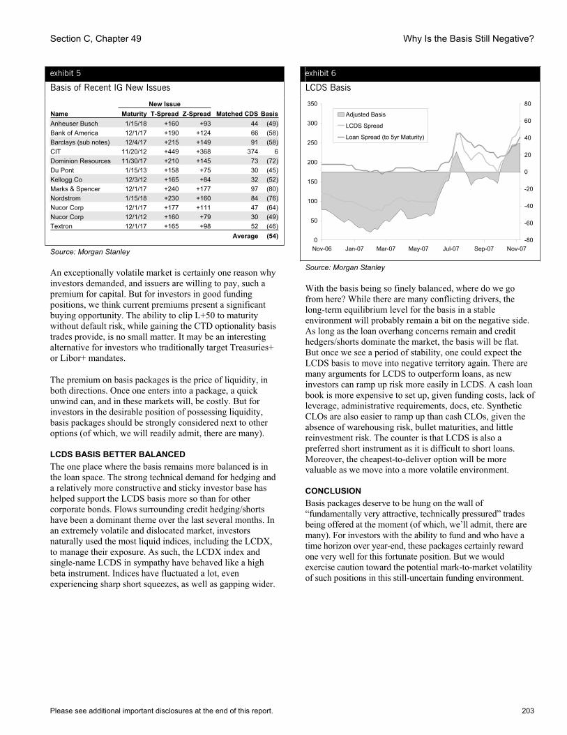
Section C, Chapter 49 Why Is the Basis Still Negative?
Please see additional important disclosures at the end of this report. 203
exhibit 5
Basis of Recent IG New Issues
New Issue Name Maturity T-Spread Z-Spread Matched CDS BasisAnheuser Busch 1/15/18 +160 +93 44 (49)Bank of America 12/1/17 +190 +124 66 (58)Barclays (sub notes) 12/4/17 +215 +149 91 (58)CIT 11/20/12 +449 +368 374 6 Dominion Resources 11/30/17 +210 +145 73 (72)Du Pont 1/15/13 +158 +75 30 (45)Kellogg Co 12/3/12 +165 +84 32 (52)Marks & Spencer 12/1/17 +240 +177 97 (80)Nordstrom 1/15/18 +230 +160 84 (76)Nucor Corp 12/1/17 +177 +111 47 (64)Nucor Corp 12/1/12 +160 +79 30 (49)Textron 12/1/17 +165 +98 52 (46) Average (54)
Source: Morgan Stanley
An exceptionally volatile market is certainly one reason why investors demanded, and issuers are willing to pay, such a premium for capital. But for investors in good funding positions, we think current premiums present a significant buying opportunity. The ability to clip L+50 to maturity without default risk, while gaining the CTD optionality basis trades provide, is no small matter. It may be an interesting alternative for investors who traditionally target Treasuries+ or Libor+ mandates.
The premium on basis packages is the price of liquidity, in both directions. Once one enters into a package, a quick unwind can, and in these markets will, be costly. But for investors in the desirable position of possessing liquidity, basis packages should be strongly considered next to other options (of which, we will readily admit, there are many).
LCDS BASIS BETTER BALANCED The one place where the basis remains more balanced is in the loan space. The strong technical demand for hedging and a relatively more constructive and sticky investor base has helped support the LCDS basis more so than for other corporate bonds. Flows surrounding credit hedging/shorts have been a dominant theme over the last several months. In an extremely volatile and dislocated market, investors naturally used the most liquid indices, including the LCDX, to manage their exposure. As such, the LCDX index and single-name LCDS in sympathy have behaved like a high beta instrument. Indices have fluctuated a lot, even experiencing sharp short squeezes, as well as gapping wider.
exhibit 6
LCDS Basis
0
50
100
150
200
250
300
350
Nov-06 Jan-07 Mar-07 May-07 Jul-07 Sep-07 Nov-07-80
-60
-40
-20
0
20
40
60
80
Adjusted Basis
LCDS Spread
Loan Spread (to 5yr Maturity)
Source: Morgan Stanley
With the basis being so finely balanced, where do we go from here? While there are many conflicting drivers, the long-term equilibrium level for the basis in a stable environment will probably remain a bit on the negative side. As long as the loan overhang concerns remain and credit hedgers/shorts dominate the market, the basis will be flat. But once we see a period of stability, one could expect the LCDS basis to move into negative territory again. There are many arguments for LCDS to outperform loans, as new investors can ramp up risk more easily in LCDS. A cash loan book is more expensive to set up, given funding costs, lack of leverage, administrative requirements, docs, etc. Synthetic CLOs are also easier to ramp up than cash CLOs, given the absence of warehousing risk, bullet maturities, and little reinvestment risk. The counter is that LCDS is also a preferred short instrument as it is difficult to short loans. Moreover, the cheapest-to-deliver option will be more valuable as we move into a more volatile environment.
CONCLUSIONBasis packages deserve to be hung on the wall of “fundamentally very attractive, technically pressured” trades being offered at the moment (of which, we’ll admit, there are many). For investors with the ability to fund and who have a time horizon over year-end, these packages certainly reward one very well for this fortunate position. But we would exercise caution toward the potential mark-to-market volatility of such positions in this still-uncertain funding environment.


Section D
Credit Curves
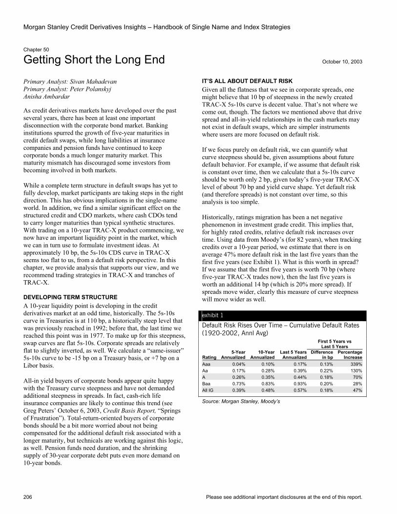
Morgan Stanley Credit Derivatives Insights – Handbook of Single Name and Index Strategies
206 Please see additional important disclosures at the end of this report.
Chapter 50
Getting Short the Long End October 10, 2003
Primary Analyst: Sivan Mahadevan Primary Analyst: Peter Polanskyj Anisha Ambardar
As credit derivatives markets have developed over the past several years, there has been at least one important disconnection with the corporate bond market. Banking institutions spurred the growth of five-year maturities in credit default swaps, while long liabilities at insurance companies and pension funds have continued to keep corporate bonds a much longer maturity market. This maturity mismatch has discouraged some investors from becoming involved in both markets.
While a complete term structure in default swaps has yet to fully develop, market participants are taking steps in the right direction. This has obvious implications in the single-name world. In addition, we find a similar significant effect on the structured credit and CDO markets, where cash CDOs tend to carry longer maturities than typical synthetic structures. With trading on a 10-year TRAC-X product commencing, we now have an important liquidity point in the market, which we can in turn use to formulate investment ideas. At approximately 10 bp, the 5s-10s CDS curve in TRAC-X seems too flat to us, from a default risk perspective. In this chapter, we provide analysis that supports our view, and we recommend trading strategies in TRAC-X and tranches of TRAC-X.
DEVELOPING TERM STRUCTURE A 10-year liquidity point is developing in the credit derivatives market at an odd time, historically. The 5s-10s curve in Treasuries is at 110 bp, a historically steep level that was previously reached in 1992; before that, the last time we reached this point was in 1977. To make up for this steepness, swap curves are flat 5s-10s. Corporate spreads are relatively flat to slightly inverted, as well. We calculate a “same-issuer” 5s-10s curve to be -15 bp on a Treasury basis, or +7 bp on a Libor basis.
All-in yield buyers of corporate bonds appear quite happy with the Treasury curve steepness and have not demanded additional steepness in spreads. In fact, cash-rich life insurance companies are likely to continue this trend (see Greg Peters’ October 6, 2003, Credit Basis Report, “Springs of Frustration”). Total-return-oriented buyers of corporate bonds should be a bit more worried about not being compensated for the additional default risk associated with a longer maturity, but technicals are working against this logic, as well. Pension funds need duration, and the shrinking supply of 30-year corporate debt puts even more demand on 10-year bonds.
IT’S ALL ABOUT DEFAULT RISK Given all the flatness that we see in corporate spreads, one might believe that 10 bp of steepness in the newly created TRAC-X 5s-10s curve is decent value. That’s not where we come out, though. The factors we mentioned above that drive spread and all-in-yield relationships in the cash markets may not exist in default swaps, which are simpler instruments where users are more focused on default risk.
If we focus purely on default risk, we can quantify what curve steepness should be, given assumptions about future default behavior. For example, if we assume that default risk is constant over time, then we calculate that a 5s-10s curve should be worth only 2 bp, given today’s five-year TRAC-X level of about 70 bp and yield curve shape. Yet default risk (and therefore spreads) is not constant over time, so this analysis is too simple.
Historically, ratings migration has been a net negative phenomenon in investment grade credit. This implies that, for highly rated credits, relative default risk increases over time. Using data from Moody’s (for 82 years), when tracking credits over a 10-year period, we estimate that there is on average 47% more default risk in the last five years than the first five years (see Exhibit 1). What is this worth in spread? If we assume that the first five years is worth 70 bp (where five-year TRAC-X trades now), then the last five years is worth an additional 14 bp (which is 20% more spread). If spreads move wider, clearly this measure of curve steepness will move wider as well.
exhibit 1
Default Risk Rises Over Time – Cumulative Default Rates (1920-2002, Annl Avg)
First 5 Years vs Last 5 Years
Rating5-Year
Annualized10-Year
AnnualizedLast 5 Years Annualized
Difference in bp
Percentage Increase
Aaa 0.04% 0.10% 0.17% 0.13% 339%Aa 0.17% 0.28% 0.39% 0.22% 130%A 0.26% 0.35% 0.44% 0.18% 70%Baa 0.73% 0.83% 0.93% 0.20% 28%All IG 0.39% 0.48% 0.57% 0.18% 47%
Source: Morgan Stanley, Moody’s
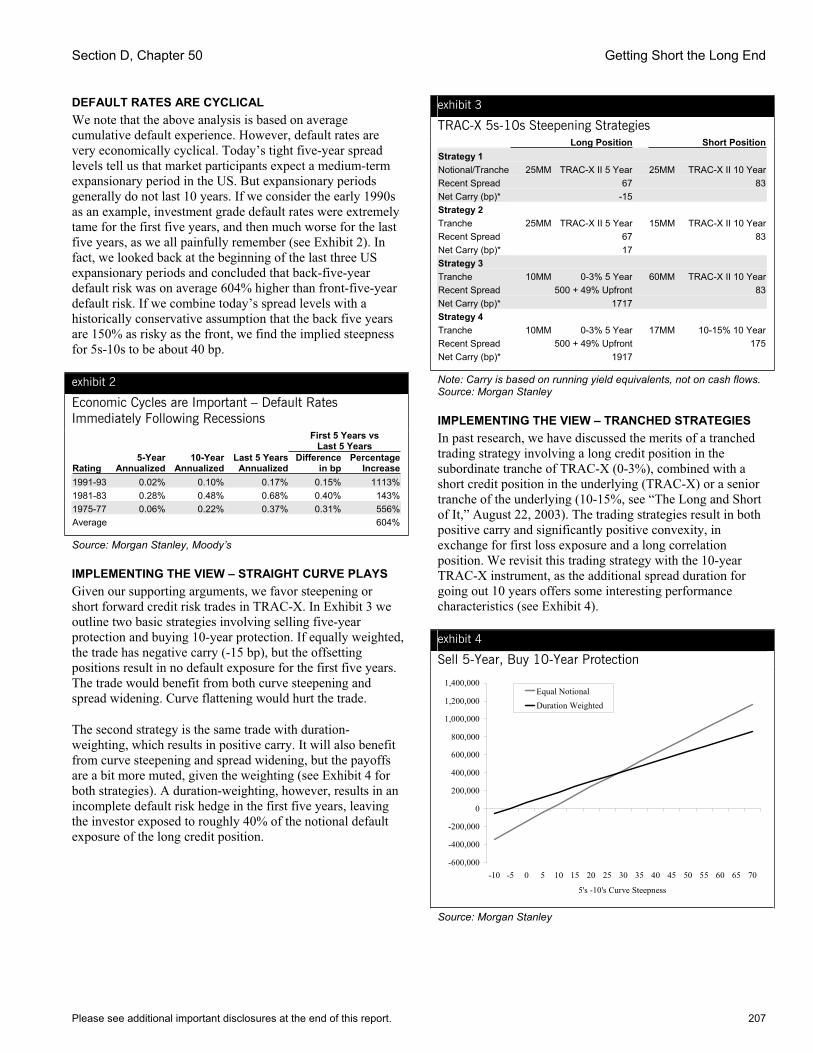
Section D, Chapter 50 Getting Short the Long End
Please see additional important disclosures at the end of this report. 207
DEFAULT RATES ARE CYCLICAL We note that the above analysis is based on average cumulative default experience. However, default rates are very economically cyclical. Today’s tight five-year spread levels tell us that market participants expect a medium-term expansionary period in the US. But expansionary periods generally do not last 10 years. If we consider the early 1990s as an example, investment grade default rates were extremely tame for the first five years, and then much worse for the last five years, as we all painfully remember (see Exhibit 2). In fact, we looked back at the beginning of the last three US expansionary periods and concluded that back-five-year default risk was on average 604% higher than front-five-year default risk. If we combine today’s spread levels with a historically conservative assumption that the back five years are 150% as risky as the front, we find the implied steepness for 5s-10s to be about 40 bp.
exhibit 2
Economic Cycles are Important – Default Rates Immediately Following Recessions
First 5 Years vs
Last 5 Years
Rating 5-Year
Annualized 10-Year
Annualized Last 5 Years Annualized
Difference in bp
Percentage Increase
1991-93 0.02% 0.10% 0.17% 0.15% 1113%1981-83 0.28% 0.48% 0.68% 0.40% 143%1975-77 0.06% 0.22% 0.37% 0.31% 556%Average 604%
Source: Morgan Stanley, Moody’s
IMPLEMENTING THE VIEW – STRAIGHT CURVE PLAYS Given our supporting arguments, we favor steepening or short forward credit risk trades in TRAC-X. In Exhibit 3 we outline two basic strategies involving selling five-year protection and buying 10-year protection. If equally weighted, the trade has negative carry (-15 bp), but the offsetting positions result in no default exposure for the first five years. The trade would benefit from both curve steepening and spread widening. Curve flattening would hurt the trade.
The second strategy is the same trade with duration-weighting, which results in positive carry. It will also benefit from curve steepening and spread widening, but the payoffs are a bit more muted, given the weighting (see Exhibit 4 for both strategies). A duration-weighting, however, results in an incomplete default risk hedge in the first five years, leaving the investor exposed to roughly 40% of the notional default exposure of the long credit position.
exhibit 3
TRAC-X 5s-10s Steepening Strategies Long Position Short PositionStrategy 1 Notional/Tranche 25MM TRAC-X II 5 Year 25MM TRAC-X II 10 YearRecent Spread 67 83Net Carry (bp)* -15Strategy 2 Tranche 25MM TRAC-X II 5 Year 15MM TRAC-X II 10 YearRecent Spread 67 83Net Carry (bp)* 17 Strategy 3 Tranche 10MM 0-3% 5 Year 60MM TRAC-X II 10 YearRecent Spread 500 + 49% Upfront 83Net Carry (bp)* 1717Strategy 4 Tranche 10MM 0-3% 5 Year 17MM 10-15% 10 Year Recent Spread 500 + 49% Upfront 175Net Carry (bp)* 1917
Note: Carry is based on running yield equivalents, not on cash flows. Source: Morgan Stanley
IMPLEMENTING THE VIEW – TRANCHED STRATEGIES In past research, we have discussed the merits of a tranched trading strategy involving a long credit position in the subordinate tranche of TRAC-X (0-3%), combined with a short credit position in the underlying (TRAC-X) or a senior tranche of the underlying (10-15%, see “The Long and Short of It,” August 22, 2003). The trading strategies result in both positive carry and significantly positive convexity, in exchange for first loss exposure and a long correlation position. We revisit this trading strategy with the 10-year TRAC-X instrument, as the additional spread duration for going out 10 years offers some interesting performance characteristics (see Exhibit 4).
exhibit 4
Sell 5-Year, Buy 10-Year Protection
-600,000
-400,000
-200,000
0
200,000
400,000
600,000
800,000
1,000,000
1,200,000
1,400,000
-10 -5 0 5 10 15 20 25 30 35 40 45 50 55 60 65 70
5's -10's Curve Steepness
Equal Notional Duration Weighted
Source: Morgan Stanley
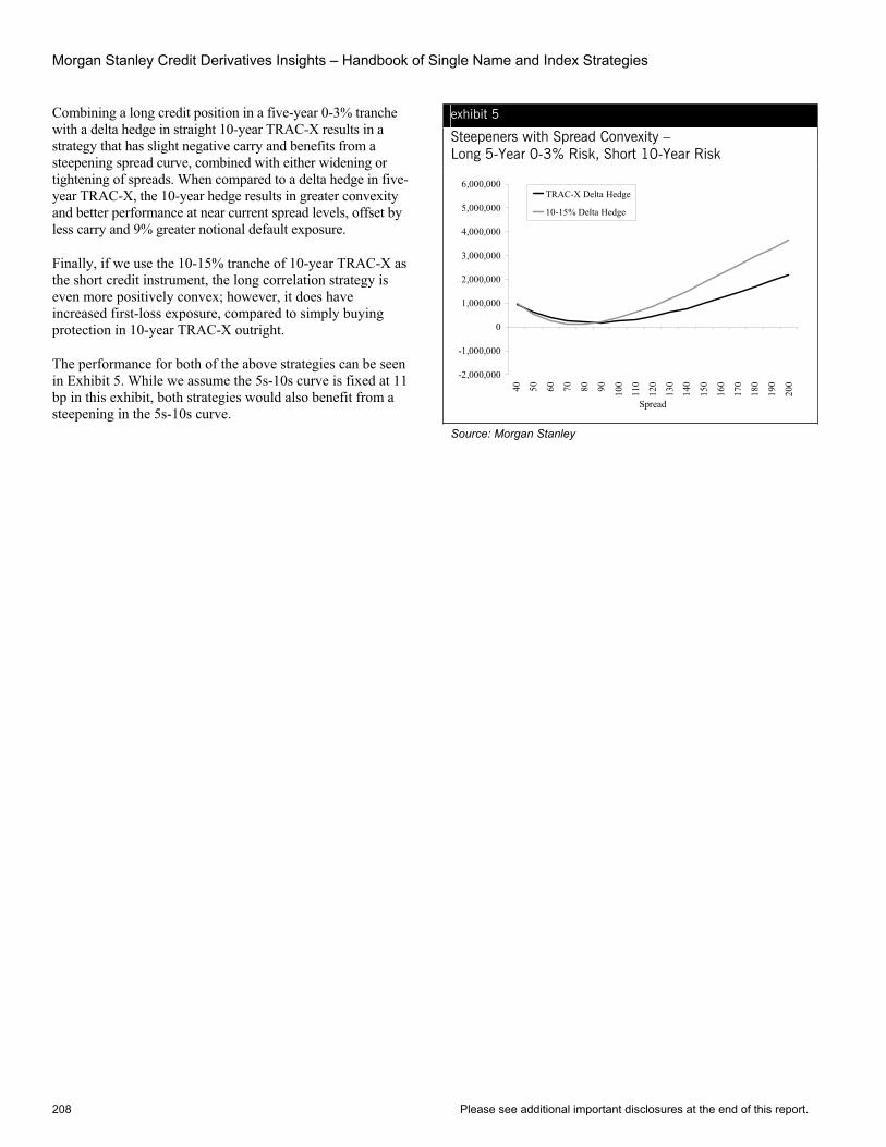
Morgan Stanley Credit Derivatives Insights – Handbook of Single Name and Index Strategies
208 Please see additional important disclosures at the end of this report.
Combining a long credit position in a five-year 0-3% tranche with a delta hedge in straight 10-year TRAC-X results in a strategy that has slight negative carry and benefits from a steepening spread curve, combined with either widening or tightening of spreads. When compared to a delta hedge in five-year TRAC-X, the 10-year hedge results in greater convexity and better performance at near current spread levels, offset by less carry and 9% greater notional default exposure.
Finally, if we use the 10-15% tranche of 10-year TRAC-X as the short credit instrument, the long correlation strategy is even more positively convex; however, it does have increased first-loss exposure, compared to simply buying protection in 10-year TRAC-X outright.
The performance for both of the above strategies can be seen in Exhibit 5. While we assume the 5s-10s curve is fixed at 11 bp in this exhibit, both strategies would also benefit from a steepening in the 5s-10s curve.
exhibit 5
Steepeners with Spread Convexity – Long 5-Year 0-3% Risk, Short 10-Year Risk
-2,000,000
-1,000,000
0
1,000,000
2,000,000
3,000,000
4,000,000
5,000,000
6,000,000
40 50 60 70 80 90 100
110
120
130
140
150
160
170
180
190
200
Spread
TRAC-X Delta Hedge
10-15% Delta Hedge
Source: Morgan Stanley
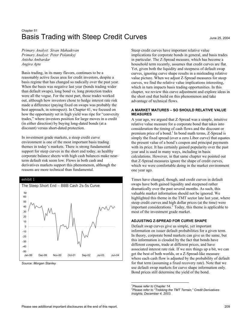
Please see additional important disclosures at the end of this report. 209
Chapter 51
Basis Trading with Steep Credit Curves June 25, 2004
Primary Analyst: Sivan Mahadevan Primary Analyst: Peter Polanskyj Anisha Ambardar Angira Apte
Basis trading, in its many flavors, continues to be a reasonably active focus area for credit investors, despite a basis regime that has changed so radically over the past year. When the basis was negative last year (bonds trading wider than default swaps), long bond vs. long protection trades were all the vogue. For the most part, those trades worked out, although how investors chose to hedge interest rate risk made a difference (paying fixed on swaps was probably the best approach, in retrospect). In Chapter 41, we focused on how the opportunity set in high yield was ripe for “convexity trades,” where investors position for large moves in a credit (in either direction) by buying long-dated bonds (at a discount) versus short-dated protection.
In investment grade markets, a steep credit curve environment is one of the most important basis trading themes in today’s markets. There is strong fundamental support for steep curves in the short end today, as healthy corporate balance sheets with high cash balances make near-term default risk seem low. Flows in both cash and derivatives markets support this phenomenon, although the reasons are more technical than fundamental.
exhibit 1
The Steep Short End – BBB Cash 2s-5s Curve
bp
-50
-40
-30
-20
-10
0
10
20
30
40
50
60
Jan-99 Dec-99 Nov-00 Oct-01 Sep-02 Jul-03 Jun-04
Source: Morgan Stanley
Steep credit curves have important relative value implications for corporate bonds in general, and basis trades in particular. The Z-Spread measure, which has become a household term recently, assumes that credit curves are flat. Yet, given both the liquidity and steepness of default swap curves, ignoring curve shape results in a misleading relative value picture. When we adjust Z-Spread measures for steep curves, we find the relative value implications interesting, which in turn impacts basis trading opportunities. In this chapter, we review this curve adjustment and explore ideas in the short end that build on this phenomenon and take advantage of technical flows.
A MARKET MATURES – SO SHOULD RELATIVE VALUE MEASURES A year ago, we argued that Z-Spread was a simple, intuitive relative value measure for a corporate bond that takes into consideration the timing of cash flows and the discount or premium price of a bond.1 In bond math terms, Z-Spread is simply the fixed spread (over a zero Libor curve) that equates the present value of a bond’s coupon and principal payments with its price. It has certainly gained popularity over the past year and is used in many ways, including in basis calculations. However, in that same chapter we pointed out that Z-Spread measures ignore the shape of credit curves, which we were comfortable doing in the market environment one year ago.
Times have changed, though, and credit curves in default swaps have both gained liquidity and steepened rather dramatically over the past several months. As such, this valuable market information should not be ignored. We highlighted this theme in the TMT sector late last year, where steep credit curves and high dollar prices (at the time) were important considerations.2 Today, this theme is applicable to most of the investment grade market.
ADJUSTING Z-SPREAD FOR CURVE SHAPE Default swap curves give us simple, yet important information on issuer default probabilities for a given term. In theory, corporate bond markets can give us the same, but this information is clouded by the fact that bonds have different coupons, trade at different prices, and have associated interest rate risk. If we mix things up a bit, we can get the best of both worlds, or a Z-Spread-like measure where each cash flow is adjusted by the probability of default for that term (assuming a fixed recovery rate). Note that we use default swap markets for curve shape information only. Bond prices still determine the yield of the bond.
1Please refer to Chapter 14. 2Please refer to “Trekking the TMT Terrain,” Credit Derivatives Insights, December 4, 2003.
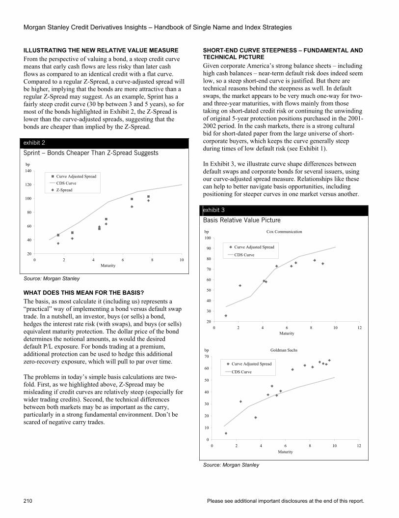
Morgan Stanley Credit Derivatives Insights – Handbook of Single Name and Index Strategies
210 Please see additional important disclosures at the end of this report.
ILLUSTRATING THE NEW RELATIVE VALUE MEASURE From the perspective of valuing a bond, a steep credit curve means that early cash flows are less risky than later cash flows as compared to an identical credit with a flat curve. Compared to a regular Z-Spread, a curve-adjusted spread will be higher, implying that the bonds are more attractive than a regular Z-Spread may suggest. As an example, Sprint has a fairly steep credit curve (30 bp between 3 and 5 years), so for most of the bonds highlighted in Exhibit 2, the Z-Spread is lower than the curve-adjusted spreads, suggesting that the bonds are cheaper than implied by the Z-Spread.
exhibit 2
Sprint – Bonds Cheaper Than Z-Spread Suggests
bp
20
40
60
80
100
120
140
0 2 4 6 8 10Maturity
Curve Adjusted SpreadCDS CurveZ-Spread
Source: Morgan Stanley
WHAT DOES THIS MEAN FOR THE BASIS? The basis, as most calculate it (including us) represents a “practical” way of implementing a bond versus default swap trade. In a nutshell, an investor, buys (or sells) a bond, hedges the interest rate risk (with swaps), and buys (or sells) equivalent maturity protection. The dollar price of the bond determines the notional amounts, as would the desired default P/L exposure. For bonds trading at a premium, additional protection can be used to hedge this additional zero-recovery exposure, which will pull to par over time.
The problems in today’s simple basis calculations are two-fold. First, as we highlighted above, Z-Spread may be misleading if credit curves are relatively steep (especially for wider trading credits). Second, the technical differences between both markets may be as important as the carry, particularly in a strong fundamental environment. Don’t be scared of negative carry trades.
SHORT-END CURVE STEEPNESS – FUNDAMENTAL AND TECHNICAL PICTURE Given corporate America’s strong balance sheets – including high cash balances – near-term default risk does indeed seem low, so a steep short-end curve is justified. But there are technical reasons behind the steepness as well. In default swaps, the market appears to be very much one-way for two- and three-year maturities, with flows mainly from those taking on short-dated credit risk or continuing the unwinding of original 5-year protection positions purchased in the 2001-2002 period. In the cash markets, there is a strong cultural bid for short-dated paper from the large universe of short-corporate buyers, which keeps the curve generally steep during times of low default risk (see Exhibit 1).
In Exhibit 3, we illustrate curve shape differences between default swaps and corporate bonds for several issuers, using our curve-adjusted spread measure. Relationships like these can help to better navigate basis opportunities, including positioning for steeper curves in one market versus another.
exhibit 3
Basis Relative Value Picture
Cox Communication
20
30
40
50
60
70
80
90
100
0 2 4 6 8 10 12Maturity
bp
Curve Adjusted Spread
CDS Curve
Goldman Sachs
0
10
20
30
40
50
60
70
0 2 4 6 8 10 12Maturity
bp
Curve Adjusted Spread
CDS Curve
Source: Morgan Stanley

Section D, Chapter 51 Basis Trading with Steep Credit Curves
Please see additional important disclosures at the end of this report. 211
LIVING WITH STEEP CREDIT CURVES To summarize our thoughts from above in a more actionable framework, we find several themes that should help credit investors position in a steep credit curve environment. In particular, for at least a handful of issuers, we support the idea of going long five-year credit risk in bonds and buying short-dated protection, for the following reasons.
• If credit curves remain steep, then owning five-year credit risk and positioning for the roll down is attractive.
• If credit curves flatten, owning five-year paper versus shorter-dated risk makes sense.
• Over a medium-term horizon, five-year bonds could outperform five-year default swaps (even if they are lower spread today) because of the strong technical demand for short-dated corporate paper. Our curve shape implied relative value measures demonstrate this richness today.
• The short end of the default swap market continues to be one way (takers of credit risk), so buyers of protection would be easily welcomed.
We find numerous examples where investors are paid well for owning the back two years of five-year credit risk (i.e., 2-year risk, three years forward).
We list two opportunities in Exhibit 4, where taking 5-year like risk in bonds may benefit from curve shape, and furthermore, the use of 3-year protection would create attractive payouts for owning just the back end of credit risk (i.e., forward long). For example, in Goldman Sachs, 5-year bonds versus 3-year protection would earn 16 bp for the hedged period (3 years) and 45 bp for the unhedged period (last 2 years). The weighted average of those premiums is 27 bp (for 5 years), or 70 bp for the back two years.
exhibit 4
Paid Well to Own the Back Years of Default Risk? Implied Spreads Ticker Instrument Maturity Spread Hedged Period Unhedged Period Weighted Average Forward PeriodGS 6.65's of 2009 4.9 45
3 Year CDS* 3.0 29Net 1.9 16 45 27 70
FON 7.625's of 2011 6.6 99 3 Year CDS* 3.0 72 Net 3.6 27 99 66 121
*CDS premium is notionally adjusted to bond dollar price Source: Morgan Stanley
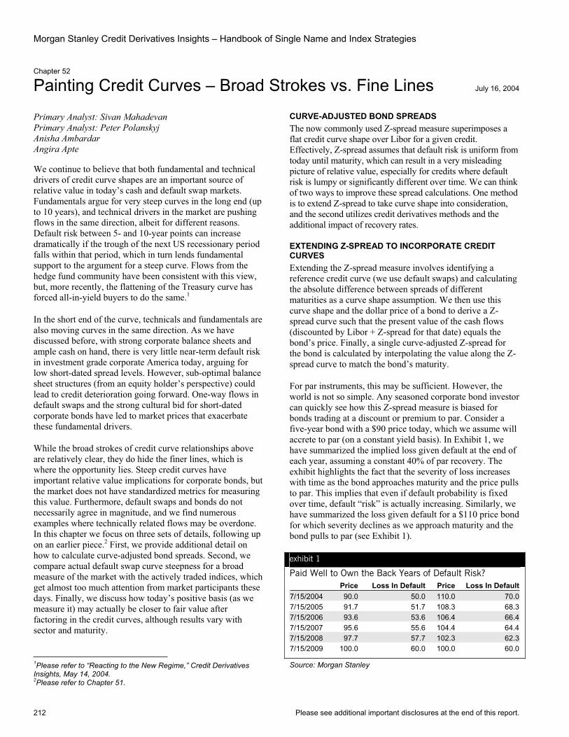
Morgan Stanley Credit Derivatives Insights – Handbook of Single Name and Index Strategies
212 Please see additional important disclosures at the end of this report.
Chapter 52
Painting Credit Curves – Broad Strokes vs. Fine Lines July 16, 2004
Primary Analyst: Sivan Mahadevan Primary Analyst: Peter Polanskyj Anisha Ambardar Angira Apte
We continue to believe that both fundamental and technical drivers of credit curve shapes are an important source of relative value in today’s cash and default swap markets. Fundamentals argue for very steep curves in the long end (up to 10 years), and technical drivers in the market are pushing flows in the same direction, albeit for different reasons. Default risk between 5- and 10-year points can increase dramatically if the trough of the next US recessionary period falls within that period, which in turn lends fundamental support to the argument for a steep curve. Flows from the hedge fund community have been consistent with this view, but, more recently, the flattening of the Treasury curve has forced all-in-yield buyers to do the same.1
In the short end of the curve, technicals and fundamentals are also moving curves in the same direction. As we have discussed before, with strong corporate balance sheets and ample cash on hand, there is very little near-term default risk in investment grade corporate America today, arguing for low short-dated spread levels. However, sub-optimal balance sheet structures (from an equity holder’s perspective) could lead to credit deterioration going forward. One-way flows in default swaps and the strong cultural bid for short-dated corporate bonds have led to market prices that exacerbate these fundamental drivers.
While the broad strokes of credit curve relationships above are relatively clear, they do hide the finer lines, which is where the opportunity lies. Steep credit curves have important relative value implications for corporate bonds, but the market does not have standardized metrics for measuring this value. Furthermore, default swaps and bonds do not necessarily agree in magnitude, and we find numerous examples where technically related flows may be overdone. In this chapter we focus on three sets of details, following up on an earlier piece.2 First, we provide additional detail on how to calculate curve-adjusted bond spreads. Second, we compare actual default swap curve steepness for a broad measure of the market with the actively traded indices, which get almost too much attention from market participants these days. Finally, we discuss how today’s positive basis (as we measure it) may actually be closer to fair value after factoring in the credit curves, although results vary with sector and maturity.
1Please refer to “Reacting to the New Regime,” Credit Derivatives Insights, May 14, 2004. 2Please refer to Chapter 51.
CURVE-ADJUSTED BOND SPREADS The now commonly used Z-spread measure superimposes a flat credit curve shape over Libor for a given credit. Effectively, Z-spread assumes that default risk is uniform from today until maturity, which can result in a very misleading picture of relative value, especially for credits where default risk is lumpy or significantly different over time. We can think of two ways to improve these spread calculations. One method is to extend Z-spread to take curve shape into consideration, and the second utilizes credit derivatives methods and the additional impact of recovery rates.
EXTENDING Z-SPREAD TO INCORPORATE CREDIT CURVESExtending the Z-spread measure involves identifying a reference credit curve (we use default swaps) and calculating the absolute difference between spreads of different maturities as a curve shape assumption. We then use this curve shape and the dollar price of a bond to derive a Z-spread curve such that the present value of the cash flows (discounted by Libor + Z-spread for that date) equals the bond’s price. Finally, a single curve-adjusted Z-spread for the bond is calculated by interpolating the value along the Z-spread curve to match the bond’s maturity.
For par instruments, this may be sufficient. However, the world is not so simple. Any seasoned corporate bond investor can quickly see how this Z-spread measure is biased for bonds trading at a discount or premium to par. Consider a five-year bond with a $90 price today, which we assume will accrete to par (on a constant yield basis). In Exhibit 1, we have summarized the implied loss given default at the end of each year, assuming a constant 40% of par recovery. The exhibit highlights the fact that the severity of loss increases with time as the bond approaches maturity and the price pulls to par. This implies that even if default probability is fixed over time, default “risk” is actually increasing. Similarly, we have summarized the loss given default for a $110 price bond for which severity declines as we approach maturity and the bond pulls to par (see Exhibit 1).
exhibit 1
Paid Well to Own the Back Years of Default Risk? Price Loss In Default Price Loss In Default7/15/2004 90.0 50.0 110.0 70.07/15/2005 91.7 51.7 108.3 68.37/15/2006 93.6 53.6 106.4 66.47/15/2007 95.6 55.6 104.4 64.47/15/2008 97.7 57.7 102.3 62.37/15/2009 100.0 60.0 100.0 60.0
Source: Morgan Stanley

Section D, Chapter 52 Painting Credit Curves – Broad Strokes vs. Fine Lines
Please see additional important disclosures at the end of this report. 213
A MORE GENERALIZED CURVE-ADJUSTED SPREAD In a nutshell, our curve-adjusted Z-spread reflects the change in probability but not the change in loss severity. We address this additional hurdle by switching to a credit derivative pricing framework to value the bonds. This framework allows us to make an explicit recovery assumption (as a percentage of par), thereby reflecting both the discount/premium nature of cash instruments and default probability curve over the life of the bond. We call this curve-adjusted par spread (CAPS).
In Exhibit 2 we summarize four spread measures for the Sprint Corp. credit curve: CDS premium, flat Z-spread (calculated from Bloomberg), curve-adjusted Z-spread, and the CAPS. The CDS curve is clearly upward sloping and all of the bonds are premium instruments. The graph highlights the fact that using a flat Z-spread makes bonds appear richer than both curve-adjusted measures. The difference between the two curve-adjusted spread measures is driven by the specific recovery assumption made in the curve-adjusted par spread (we can think of Z-spread as a measure that effectively assumes a zero recovery rate).
exhibit 2
Sprint Corp. – Curve Shape and Dollar Price Matter
0
50
100
150
0 2 4 6 8 10
Curve Adj Z- Spread
CDS Spread
Curve Adj Par Spread
Flat Z-Spread
Source: Morgan Stanley
HOW STEEP? HYPER LIQUIDITY VS. THE REST OF THE MARKET There is a lot of fairly valuable information in default swap credit curves today, as we see from the above analysis. Yet, when making broad statements about the market, there is too much focus by market participants on the indices, given how easy it is to glance at the numerous Bloomberg runs. While it is true that the indices capture a reasonable portion of the market, we should not ignore the fact they also exclude a significant part of the market. Furthermore, the liquidity differences between single names and the indices have important valuation implications.
One exercise we find intriguing is actually comparing the hyper liquid indices with the rest of the market. For example, using a universe of approximately 225 credits, we find that the 5s-10s curve is a bit flatter (14 bp mid-market, see Exhibit 3) than in CDX (where it is 20 bp and markets trade almost locked). The same is true if we just focus on the 125 CDX single names against the traded index, although bid-offer can make the arbitrage uneconomical.
exhibit 3
Varying Steepness – Default Swap Credit Curve Shape
Sector5-Year
CDSCDS 3s-5s
Curve CDS 5s-10s
Curve Consumer Discretionary 54 10 15Consumer Staples 41 5 15Energy 46 9 12Financial: Banks 31 8 12Financial: Non-banks 64 7 10Health Care 39 6 13Industrials 43 9 12Information Technology 61 13 17Materials 45 12 15Telecommunication Services 86 25 25Utilities 59 10 12Total 52 9 14
CDX 61 NA 20
Note: 225 name universe Source: Morgan Stanley
SECTOR CREDIT CURVE THEMES Among sectors captured in the 225-name universe summarized in Exhibit 3, Telecom is the steepest at 25 bp, although it is also the widest in average spread. AT&T’s curve accounts for 4 of the 25 bp. The remaining sectors have very little dispersion, which we believe is related to poorer liquidity at the 10-year point. The 3s-5s curve is about 10 bp on average. Telecom is the significant outlier here as well (at 25 bp with AT&T accounting for 7 of the 25 bp). Consumer Staples is the flattest curve, which we argue is related to absolute spread level and the sector’s non-cyclical nature.
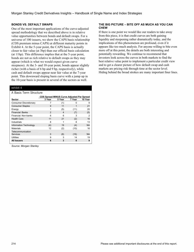
Morgan Stanley Credit Derivatives Insights – Handbook of Single Name and Index Strategies
214 Please see additional important disclosures at the end of this report.
BONDS VS. DEFAULT SWAPS One of the most important applications of the curve-adjusted spread methodology that we described above is in relative value opportunities between bonds and default swaps. For a universe of 100 issuers, we show the CAPS basis relationship (CDS premium minus CAPS) at different maturity points in Exhibit 4. At the 5-year point, the CAPS basis is actually closer to fair value (at 3bp) than our official basis calculation (at 11bp). This difference implies that at the 5-year point, bonds are not as rich relative to default swaps as they may appear (which is what we would expect given curve steepness). At the 3- and 10-year point, bonds appear slightly richer (with a basis of 6 bp and 9 bp, respectively), while cash and default swaps appear near fair value at the 7-year point. This downward sloping basis curve with a jump up in the 10-year basis is present in several of the sectors as well.
exhibit 4
A Basis Term Structure CDS Spread MINUS Curve Adjusted Par SpreadSector 3 Year 5 Year 7 Year 10 Year Consumer Discretionary 7 (1) 0 9Consumer Staples 9 11 1 21Energy 1 (5) (11) 20Financial: Banks 2 4 (7) (5)Financial: Non-banks 6 6 3 2Health Care 11 21 (2) 16Industrials 8 1 8 13Information Technology (4) 19 (4) NAMaterials 12 (2) (10) 16Telecommunication Services 0 (8) (16) NAUtilities 9 3 14 19All Issuers 6 3 0 9
Source: Morgan Stanley
THE BIG PICTURE – BITE OFF AS MUCH AS YOU CAN CHEWIf there is one point we would like our readers to take away from this piece, it is that credit curves are both gaining liquidity and steepening rather dramatically today, and the implications of this phenomenon are profound, even if it appears like too much analysis. For anyone willing to bite even more off at this point, the details are both interesting and potentially rewarding. We continue to recommend that investors look across the curves in both markets to find the best relative value point to implement a particular credit view and to get a clearer picture of how default swap and cash markets are pricing risk through time at the sector level. Hiding behind the broad strokes are many important finer lines.

Please see additional important disclosures at the end of this report. 215
Chapter 53
Curve Lessons from High Yield August 6, 2004
Primary Analyst: Sivan Mahadevan Primary Analyst: Peter Polanskyj Anisha Ambardar Angira Apte
In the single-name credit derivatives space, if there is a topic that is becoming a key theme for the year, credit curves would get our vote. The development and standardization in the index market helped jump-start credit curve trading, but macroeconomic forces and credit fundamentals have taken it to the next level. To those who regularly follow our published research, we may seem obsessed with credit curves, but our fascination stems from our view that curves are an important source of relative value in today’s credit environment.
We have discussed recently that the steepness in investment grade curves is a situation driven by technical flows and supported by credit fundamentals for many issuers.1 Near-term default risk seems low for the market at large, given cash-rich balance sheets, and long-run default risk ought to be much higher, as a turn in the economic cycle (at some point) would bring back memories of 2001 and 2002.
When do credit curve shapes represent opportunities? Beyond the macro themes, the real relative value involves taking a much closer look at a company’s operating environment, along with its debt maturity profile and any expected changes in this capital structure. In this respect, investment grade investors may be able to learn a lot from the high yield market, which exhibits a fair amount of dispersion in credit curve shapes, driven by, among other things, dissimilar debt term structures.
PIPELINE CURVES IN HIGH YIELD We highlight the following curve shape relationships in high yield to provide insight into the effect debt maturity has on curve shapes. Pipeline companies El Paso (B3/B-) and Williams Companies (B3/B+) trade at very different zip codes in 5-year default swaps (500 versus 200 area), and their credit curves take dramatically dissimilar shapes as well (see Exhibit 1). El Paso has a very flat curve after 2006, with a bit of a hump in the 4- to 5-year maturity. The market is very focused on 2005 debt payments (bonds and loans) and a busted long-dated convertible bond that can be “put” to the issuer in 2006. The slight downward-sloping curve beyond these dates reflects the sentiment, popular for stressed credits – if they make it in the near term, they will make it in the long term.
Williams Cos. makes for an interesting story, as well, as the company recently tendered much of its near-term debt. Default swap curves steepened immediately (as they should),
1Please refer to Chapter 51.
given the radically different near-term risk for the company. On a relative basis, the curve is significantly steeper than El Paso’s. Williams also announced a tender offer for 2010 maturity, which may cause the curve to steepen from that maturity point forward.
exhibit 1
Flat and Steep Pipelines – El Paso and Williams Cos.
Debt Outstanding ($MM)
0
1,000
2,000
3,000
4,000
2004 2005 2006 2007 2008 2009 2010 2011 2012 2013 20140
100
200
300
400
500
600
700CDS Premium
Bonds Loans Curve Mid
El Paso
Debt Outstanding ($MM)
0
1,000
2,000
3,000
4,000
2004 2005 2006 2007 2008 2009 2010 2011 2012 2013 20140
100
200
300
400
500
600
700CDS Premium
Bonds Loans Curve Mid
Williams Companies
Source: Morgan Stanley, Bloomberg, Company Reports

Morgan Stanley Credit Derivatives Insights – Handbook of Single Name and Index Strategies
216 Please see additional important disclosures at the end of this report.
HIGH-YIELDING PAPER CURVES Abitibi (Ba2/BB) and Bowater (Ba2/BB) are natural comparables in the paper sector as they trade at similar 5-year CDS levels and have the same ratings and leverage levels. Yet their debt maturity profiles are very different. Abitibi has relatively evenly distributed debt maturity over the next few years. After recent refinancings, Bowater has no debt due until 2009, which explains its steeper curve relative to Abitibi (30 bp for three years, and nearly 50 bp for two years). Yet one could argue that the curve should be even steeper, given the stark differences in debt maturity profile between the two issuers. But that’s not the whole story.
A poorer relative operating model for Bowater may be the force that prevents the curve from getting as steep as the debt maturity profile would imply. Away from the credits we have highlighted, there is much focus on debt payments, in general, in high yield default swap curves. The airline space is an obvious sector, given the focus by investors on a given company’s ability to survive beyond certain debt maturities.2
exhibit 2
Flat and Steep Paper – Abitibi and Bowater
Debt Outstanding ($MM)
0
100
200
300
400
500
600
700
800
900
2004 2005 2006 2007 2008 2009 2010 2011 2012 2013 20140
50
100
150
200
250
300
350CDS Premium
Bonds Loans Curve Mid
Abitibi
Debt Outstanding ($MM)
0
100
200
300
400
500
600
700
800
900
2004 2005 2006 2007 2008 2009 2010 2011 2012 2013 20140
50
100
150
200
250
300
350CDS Premium
Bonds Loans Curve Mid
Bowater
Source: Morgan Stanley, Bloomberg, Company Reports
2Please refer to Chapter 43.
ENTER INVESTMENT GRADE As we have addressed in previous research, credit curve relationships in investment grade can be very technical and are, in general, very steep today in both cash and default swaps. Flows in short-dated default swaps tend to be one-way (sellers of protection). In the cash markets, there has traditionally been a strong cultural bid in the US for short-dated paper.
Within our universe of 220 investment grade credits, 3- to 5-year default swap curves for 200 issuers are upward-sloping, with the rest being flat. The average steepness is 12 bp, with half the universe steeper than 10 bp (for just two years of incremental default risk). Not all credits, though, are worthy of such steep curves.
As an example, the credit curve of (the now investment grade) Yum! Brands (Baa3/BBB-) is relatively steep between three and five years (see Exhibit 3). Yet, Yum has a partially drawn loan facility and bonds maturing in 2005 – and then only a few small maturities before 2011-12, which we believe is an argument for a much flatter curve. Disney (Baa1/BBB+) provides another example of a credit with significant shorter-dated maturities and a meaningfully steep credit curve. On the other side of the spectrum, we find Limited Brands (Baa1/BBB+), which has no debt due before 2012 (aside from an as-yet-undrawn loan facility) and yet has a relatively flat credit curve in the same period (see Exhibit 3).
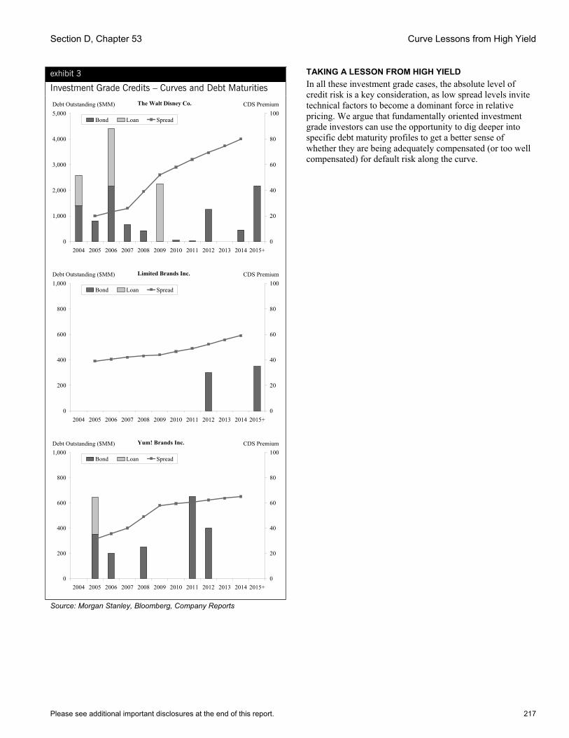
Section D, Chapter 53 Curve Lessons from High Yield
Please see additional important disclosures at the end of this report. 217
exhibit 3
Investment Grade Credits – Curves and Debt Maturities
Debt Outstanding ($MM)
0
1,000
2,000
3,000
4,000
5,000
2004 2005 2006 2007 2008 2009 2010 2011 2012 2013 2014 2015+0
20
40
60
80
100CDS Premium
Bond Loan Spread
The Walt Disney Co.
Debt Outstanding ($MM)
0
200
400
600
800
1,000
2004 2005 2006 2007 2008 2009 2010 2011 2012 2013 2014 2015+0
20
40
60
80
100CDS Premium
Bond Loan Spread
Limited Brands Inc.
Debt Outstanding ($MM)
0
200
400
600
800
1,000
2004 2005 2006 2007 2008 2009 2010 2011 2012 2013 2014 2015+0
20
40
60
80
100CDS Premium
Bond Loan Spread
Yum! Brands Inc.
Source: Morgan Stanley, Bloomberg, Company Reports
TAKING A LESSON FROM HIGH YIELD In all these investment grade cases, the absolute level of credit risk is a key consideration, as low spread levels invite technical factors to become a dominant force in relative pricing. We argue that fundamentally oriented investment grade investors can use the opportunity to dig deeper into specific debt maturity profiles to get a better sense of whether they are being adequately compensated (or too well compensated) for default risk along the curve.
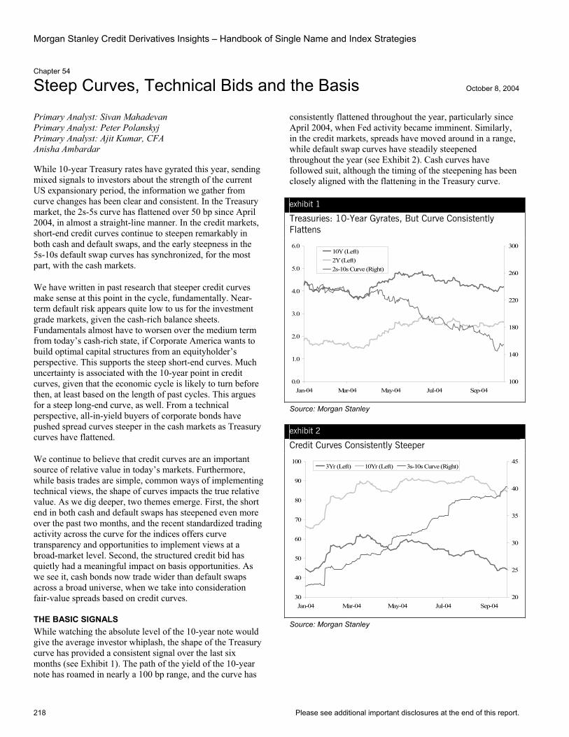
Morgan Stanley Credit Derivatives Insights – Handbook of Single Name and Index Strategies
218 Please see additional important disclosures at the end of this report.
Chapter 54
Steep Curves, Technical Bids and the Basis October 8, 2004
Primary Analyst: Sivan Mahadevan Primary Analyst: Peter Polanskyj Primary Analyst: Ajit Kumar, CFA Anisha Ambardar
While 10-year Treasury rates have gyrated this year, sending mixed signals to investors about the strength of the current US expansionary period, the information we gather from curve changes has been clear and consistent. In the Treasury market, the 2s-5s curve has flattened over 50 bp since April 2004, in almost a straight-line manner. In the credit markets, short-end credit curves continue to steepen remarkably in both cash and default swaps, and the early steepness in the 5s-10s default swap curves has synchronized, for the most part, with the cash markets.
We have written in past research that steeper credit curves make sense at this point in the cycle, fundamentally. Near-term default risk appears quite low to us for the investment grade markets, given the cash-rich balance sheets. Fundamentals almost have to worsen over the medium term from today’s cash-rich state, if Corporate America wants to build optimal capital structures from an equityholder’s perspective. This supports the steep short-end curves. Much uncertainty is associated with the 10-year point in credit curves, given that the economic cycle is likely to turn before then, at least based on the length of past cycles. This argues for a steep long-end curve, as well. From a technical perspective, all-in-yield buyers of corporate bonds have pushed spread curves steeper in the cash markets as Treasury curves have flattened.
We continue to believe that credit curves are an important source of relative value in today’s markets. Furthermore, while basis trades are simple, common ways of implementing technical views, the shape of curves impacts the true relative value. As we dig deeper, two themes emerge. First, the short end in both cash and default swaps has steepened even more over the past two months, and the recent standardized trading activity across the curve for the indices offers curve transparency and opportunities to implement views at a broad-market level. Second, the structured credit bid has quietly had a meaningful impact on basis opportunities. As we see it, cash bonds now trade wider than default swaps across a broad universe, when we take into consideration fair-value spreads based on credit curves.
THE BASIC SIGNALS While watching the absolute level of the 10-year note would give the average investor whiplash, the shape of the Treasury curve has provided a consistent signal over the last six months (see Exhibit 1). The path of the yield of the 10-year note has roamed in nearly a 100 bp range, and the curve has
consistently flattened throughout the year, particularly since April 2004, when Fed activity became imminent. Similarly, in the credit markets, spreads have moved around in a range, while default swap curves have steadily steepened throughout the year (see Exhibit 2). Cash curves have followed suit, although the timing of the steepening has been closely aligned with the flattening in the Treasury curve.
exhibit 1
Treasuries: 10-Year Gyrates, But Curve Consistently Flattens
0.0
1.0
2.0
3.0
4.0
5.0
6.0
Jan-04 Mar-04 May-04 Jul-04 Sep-04100
140
180
220
260
30010Y (Left)2Y (Left)2s-10s Curve (Right)
Source: Morgan Stanley
exhibit 2
Credit Curves Consistently Steeper
30
40
50
60
70
80
90
100
Jan-04 Mar-04 May-04 Jul-04 Sep-0420
25
30
35
40
453Yr (Left) 10Yr (Left) 3s-10s Curve (Right)
Source: Morgan Stanley
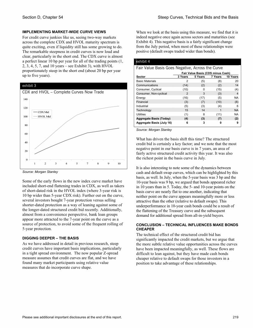
Section D, Chapter 54 Steep Curves, Technical Bids and the Basis
Please see additional important disclosures at the end of this report. 219
IMPLEMENTING MARKET-WIDE CURVE VIEWS For credit curve junkies like us, seeing two-way markets across the complete CDX and HVOL maturity spectrum is quite exciting, even if liquidity still has some growing to do. The remarkable steepness in credit curves is now loud and clear, particularly in the short end. The CDX curve is almost a perfect linear 10 bp per year for all of the trading points (1, 2, 3, 4, 5, 7, and 10 years – see Exhibit 3), with HVOL proportionately steep in the short end (about 20 bp per year up to five years).
exhibit 3
CDX and HVOL – Complete Curves Now Trade
0
20
40
60
80
100
120
140
1 2 3 4 5 7 8 9 10
CDX MidHVOL Mid
Source: Morgan Stanley
Some of the early flows in the new index curve market have included short-end flattening trades in CDX, as well as takers of short-dated risk in the HVOL index (where 3-year risk is 10 bp wider than 5-year CDX risk). Further out on the curve, several investors bought 7-year protection versus selling shorter-dated protection as a way of leaning against some of the longer-dated structured credit bid recently. Additionally, almost from a convenience perspective, bank loan groups appear more attracted to the 7-year point on the curve as a source of protection, to avoid some of the frequent rolling of 5-year protection.
DIGGING DEEPER – THE BASIS As we have addressed in detail in previous research, steep credit curves have important basis implications, particularly in a tight spread environment. The now popular Z-spread measure assumes that credit curves are flat, and we have found many market participants using relative value measures that do incorporate curve shape.
When we look at the basis using this measure, we find that it is indeed negative once again across sectors and maturities (see Exhibit 4). This negative basis is a fairly significant change from the July period, when most of these relationships were positive (default swaps traded wider than bonds).
exhibit 4
Fair Value Basis Goes Negative, Across the Curve Fair Value Basis (CDS minus Cash) Sector 3 Years 5 Years 7 Years 10 YearsBasic Materials 2 (5) (8) 20Communications (14) (2) (2) 14Consumer, Cyclical (10) 0 (15) (4)Consumer, Non-cyclical 2 3 (3) 4Energy (16) (17) (5) NAFinancial (3) (7) (10) (8)Industrial (5) (3) (4) 6Technology 15 14 1 NAUtilities (1) 8 (11) NAAggregate Basis (Today) (4) (3) (7) (2)Aggregate Basis (July 16) 6 3 0 9
Source: Morgan Stanley
What has driven the basis shift this time? The structured credit bid is certainly a key factor; and we note that the most negative point in our basis curve is in 7 years, an area of fairly active structured credit activity this year. It was also the richest point in the basis curve in July.
It is also interesting to note some of the dynamics between cash and default swap curves, which can be highlighted by this basis, as well. In July, when the 5-year basis was 3 bp and the 10-year basis was 9 bp, we argued that bonds appeared richer in 10 years than in 5. Today, the 5- and 10-year points on the basis curve are nearly flat to one another, indicating that neither point on the curve appears meaningfully more or less attractive than the other (relative to default swaps). This underperformance in 10-year cash bonds could be a result of the flattening of the Treasury curve and the subsequent demand for additional spread from all-in-yield buyers.
CONCLUSION – TECHNICAL INFLUENCES MAKE BONDS CHEAPER The technical effect of the structured credit bid has significantly impacted the credit markets, but we argue that the more subtle relative value opportunities across the curves have been impacted meaningfully, as well. These flows are difficult to lean against, but they have made cash bonds cheaper relative to default swaps for those investors in a position to take advantage of these relationships.
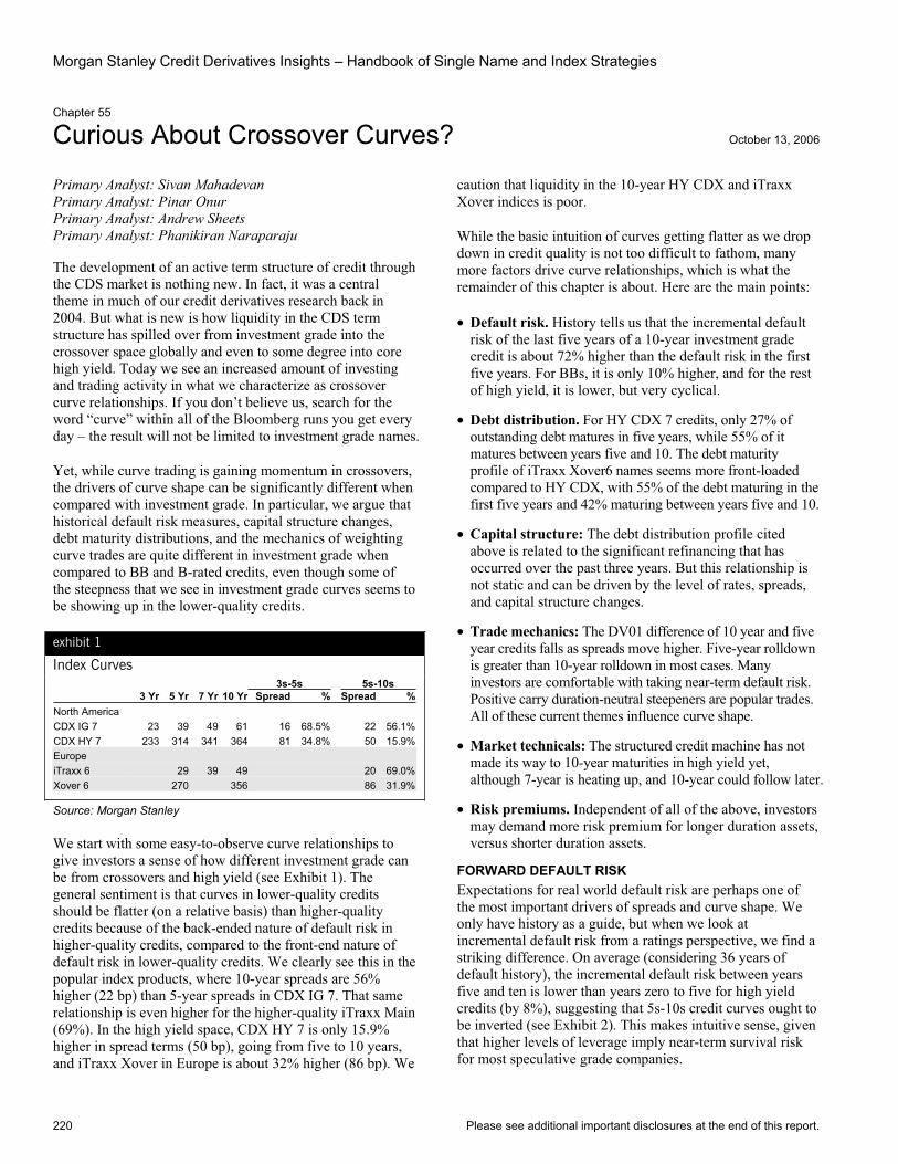
Morgan Stanley Credit Derivatives Insights – Handbook of Single Name and Index Strategies
220 Please see additional important disclosures at the end of this report.
Chapter 55
Curious About Crossover Curves? October 13, 2006
Primary Analyst: Sivan Mahadevan Primary Analyst: Pinar Onur Primary Analyst: Andrew Sheets Primary Analyst: Phanikiran Naraparaju
The development of an active term structure of credit through the CDS market is nothing new. In fact, it was a central theme in much of our credit derivatives research back in 2004. But what is new is how liquidity in the CDS term structure has spilled over from investment grade into the crossover space globally and even to some degree into core high yield. Today we see an increased amount of investing and trading activity in what we characterize as crossover curve relationships. If you don’t believe us, search for the word “curve” within all of the Bloomberg runs you get every day – the result will not be limited to investment grade names.
Yet, while curve trading is gaining momentum in crossovers, the drivers of curve shape can be significantly different when compared with investment grade. In particular, we argue that historical default risk measures, capital structure changes, debt maturity distributions, and the mechanics of weighting curve trades are quite different in investment grade when compared to BB and B-rated credits, even though some of the steepness that we see in investment grade curves seems to be showing up in the lower-quality credits.
exhibit 1
Index Curves 3s-5s 5s-10s 3 Yr 5 Yr 7 Yr 10 Yr Spread % Spread %North America CDX IG 7 23 39 49 61 16 68.5% 22 56.1%CDX HY 7 233 314 341 364 81 34.8% 50 15.9%EuropeiTraxx 6 29 39 49 20 69.0%Xover 6 270 356 86 31.9%
Source: Morgan Stanley
We start with some easy-to-observe curve relationships to give investors a sense of how different investment grade can be from crossovers and high yield (see Exhibit 1). The general sentiment is that curves in lower-quality credits should be flatter (on a relative basis) than higher-quality credits because of the back-ended nature of default risk in higher-quality credits, compared to the front-end nature of default risk in lower-quality credits. We clearly see this in the popular index products, where 10-year spreads are 56% higher (22 bp) than 5-year spreads in CDX IG 7. That same relationship is even higher for the higher-quality iTraxx Main (69%). In the high yield space, CDX HY 7 is only 15.9% higher in spread terms (50 bp), going from five to 10 years, and iTraxx Xover in Europe is about 32% higher (86 bp). We
caution that liquidity in the 10-year HY CDX and iTraxx Xover indices is poor.
While the basic intuition of curves getting flatter as we drop down in credit quality is not too difficult to fathom, many more factors drive curve relationships, which is what the remainder of this chapter is about. Here are the main points:
• Default risk. History tells us that the incremental default risk of the last five years of a 10-year investment grade credit is about 72% higher than the default risk in the first five years. For BBs, it is only 10% higher, and for the rest of high yield, it is lower, but very cyclical.
• Debt distribution. For HY CDX 7 credits, only 27% of outstanding debt matures in five years, while 55% of it matures between years five and 10. The debt maturity profile of iTraxx Xover6 names seems more front-loaded compared to HY CDX, with 55% of the debt maturing in the first five years and 42% maturing between years five and 10.
• Capital structure: The debt distribution profile cited above is related to the significant refinancing that has occurred over the past three years. But this relationship is not static and can be driven by the level of rates, spreads, and capital structure changes.
• Trade mechanics: The DV01 difference of 10 year and five year credits falls as spreads move higher. Five-year rolldown is greater than 10-year rolldown in most cases. Many investors are comfortable with taking near-term default risk. Positive carry duration-neutral steepeners are popular trades. All of these current themes influence curve shape.
• Market technicals: The structured credit machine has not made its way to 10-year maturities in high yield yet, although 7-year is heating up, and 10-year could follow later.
• Risk premiums. Independent of all of the above, investors may demand more risk premium for longer duration assets, versus shorter duration assets.
FORWARD DEFAULT RISK Expectations for real world default risk are perhaps one of the most important drivers of spreads and curve shape. We only have history as a guide, but when we look at incremental default risk from a ratings perspective, we find a striking difference. On average (considering 36 years of default history), the incremental default risk between years five and ten is lower than years zero to five for high yield credits (by 8%), suggesting that 5s-10s credit curves ought to be inverted (see Exhibit 2). This makes intuitive sense, given that higher levels of leverage imply near-term survival risk for most speculative grade companies.

Section D, Chapter 55 Curious About Crossover Curves?
Please see additional important disclosures at the end of this report. 221
exhibit 2
Incremental Default Risk Should Influence Curve Shapes % Increase 3x5 % Increase 5x5 3-Yr Annualized 5-YrAnnualized 10-Yr Annualized Last 2yrs/First 3yrs Last 5yrs/First 5yrsInv Grade 0.13% 0.18% 0.18% 91.91% 71.59%%Aaa 0.00% 0.02% 0.03% n/a 257.42%Aa 0.02% 0.05% 0.06% 353.61% 98.73%A 0.08% 0.11% 0.10% 100.17% 93.65%Baa 0.31% 0.41% 0.38% 80.39% 62.90%High Yield 3.82% 3.73% 3.16% -5.86% -7.57%Ba 1.86% 2.13% 2.26% 35.39% 9.88%B 5.97% 5.65% 5.03% -13.77% -7.91%Caa-C 15.21% 12.42% 9.11% -47.07% -37.71%
Source: Morgan Stanley, Moody’s
For investment grade, it is the other way around, where five-year default risk five years forward is 72% higher than default risk of the first five years. But from AAAs to CCCs, the forward increment falls steadily, so AAAs are the riskiest by this measure (should have the steepest relative curves) and CCCs are the least risky (should have the most inverted curves). The BB point is modestly positive (10%), while BBBs are very positive (63%). But averages can be misleading, given the cyclical nature of default risk, and if we look over time (cohorts), we find that the BBs have periods of negative forward default risk (see Exhibit 3).
exhibit 3
5s-10s Incremental Default Risk – Very Cyclical
-6.00%
-4.00%
-2.00%
0.00%
2.00%
4.00%
6.00%
8.00%
10.00%
1970
1972
1974
1976
1978
1980
1982
1984
1986
1988
1990
1992
1994
1996
Ba Incremental Default HY Incremental DefaultBa 5yr Annualized Default HY 5yr Annualized Default
Source: Morgan Stanley, Moody’s
DEBT DISTRIBUTION AND CURVES – US AND EUROPE Debt distribution for the 100 names in the HY CDX index stands in contrast to the average historical default risk numbers, placing more importance on the cyclical nature of default risk. With a great deal of high yield debt issuance over the past three years, we find that on average only 27% of the debt that HY CDX 7 companies have is due within the next five years cumulatively, while 82% is due within 10 years (a 2x increase in the last five years, see Exhibit 4).
One problem with this analysis is that debt profiles are not static, and there are other liabilities that are missing including interest payments and pension liabilities.
But ignoring this non-static component for a moment, the current debt distribution implies largely back-ended default risk, which is an argument for a steeper curve than we see in the index (50 bp or 15% of spread). However, we caution that there is very little liquidity in 10-year HY CDX, and most of the activity north of five years is in seven years, which is structured-credit related.
Aggregate debt distribution for iTraxx Xover seems more balanced. 51% percent of the outstanding debt matures in the first five years, while 42% of the debt is due between years five and 10 (see Exhibit 4). The iTraxx Xover debt distribution data call for a flatter, or even a slightly inverted curve, once again under the assumption that the current debt profile is fixed (but the curve is actually steeper than HY CDX).
exhibit 4
When Is the Debt Due? – Cumulative Debt Distribution for HY CDX 7 and iTraxx Xover 6
0%
10%
20%
30%
40%
50%
60%
70%
80%
90%
100%
1 2 3 4 5 6 7 8 9 10 11+Year
HY CDX7
iTraxx6 XO
Source: Morgan Stanley, Bloomberg

Morgan Stanley Credit Derivatives Insights – Handbook of Single Name and Index Strategies
222 Please see additional important disclosures at the end of this report.
SINGLE-NAME CURVES – EUROPE AND THE US If we look inside both the HY CDX and iTraxx Xover indices, we find that the relationships between curves and cumulative debt distribution for most credits (85-90%) are well behaved (i.e., highly correlated – in the 80-100% range, see Exhibit 5). However, we observed some divergence both in the US names (10%) and European names (~15%). Neither the ratings category nor the sector seems to be a factor in these dislocations. Clearly these dislocations drive some difference we see at the aggregate index level, along with a lack of longer-dated index liquidity.
exhibit 5
Debt Distribution and CDS Curve Correlation
0%
10%
20%
30%
40%
50%
60%
70%
50-60% 60-70% 70-80% 80-90% 90-100%Correlation Bucket
US Europe
Source: Morgan Stanley, Bloomberg
TRADE MECHANICS DRIVE CURVE SHAPES Finally, one point that we would like to drive home with this chapter is the idea that carry and rolldown on curve trades can actually drive curve relationships as much as some of the debt distribution and historical default risk relationships that we described. The inherent appeal of curve trades is the ability to trade one type of risk (default risk) for another (spread risk) and get paid accordingly. Curve positions can minimize spread risk and retain default risk and vice-versa compared with outright long or short positions in a credit. In Exhibit 6, we show four 5s-10s trades: a notional equivalent flattener and steepener, and a DV01-neutral flattener and steepener, using a “typical” crossover curve relationship that we see today (185 bp 5-year spread, 255 bp 10-year spread).
NOTIONAL WEIGHTING – SPREAD INSTEAD OF DEFAULT RISK Even notional trades effectively have no default risk over the initial period, with the trade-off being long or short duration exposure during this period. The steepener (buy 10-year protection, sell 5-year protection, same notional) has a duration mismatch of about 2.7 years (short) and is very negative carry (70 bp), which is typical of today’s crossover curves. The notionally weighted flattener is the exact opposite.
DURATION WEIGHTING – DEFAULT INSTEAD OF SPREAD RISK Doing the trades on a duration-weighted basis makes the position much less sensitive to parallel shifts in spreads, but there is exposure to curve reshapings. The trade-off is default risk during the life of the trade. The duration weighted steepener pays better (positive carry 28 bp and better rolldown 161 bp) than the notional weighted steepener as we are buying less protection on the long-end and taking on default risk in the process. The flattener has worse economics (negative carry of 45 bp and rolldown of -261 bp) as it is short default risk. In both of these cases, we are assuming that the curves remain unchanged. However, the forward credit curve would actually flatten over time, making both trades roughly equivalent, if forwards are realized. The duration-neutral steepener is popular in the market today because of the carry and rolldown and the notion that many investors are comfortable taking near-term default risk. Investors are in fact leaning against the forwards.
One way to manage this default exposure is to buy/sell short-dated protection to the residual notional (for example, buy 3.8MM 1-year protection for the duration-weighted steepener). Conversely the 5s/10s flattener benefits in a default scenario, and one way to 'monetize' this positive jump-to-default exposure is by selling 1-year protection (sell 6.2MM 10-year protection for the duration-weighted flattener).
We remind investors that durations can clearly drift over time. The steepener is duration-neutral initially but gradually gets short the market because the 5-year duration drops at a faster rate relative to 10-year duration. Conversely, the flattener gradually becomes long the market.
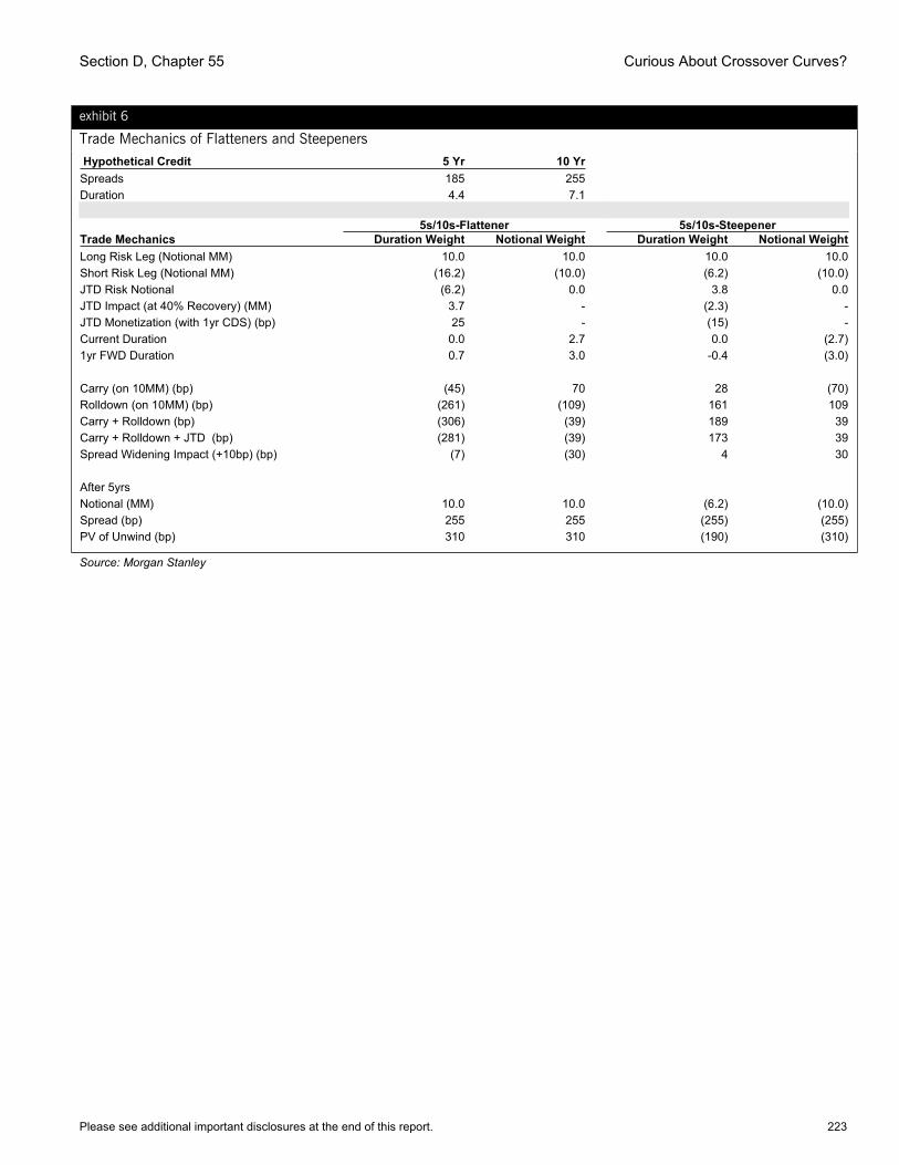
Section D, Chapter 55 Curious About Crossover Curves?
Please see additional important disclosures at the end of this report. 223
exhibit 6
Trade Mechanics of Flatteners and Steepeners Hypothetical Credit 5 Yr 10 YrSpreads 185 255 Duration 4.4 7.1
5s/10s-Flattener 5s/10s-Steepener Trade Mechanics Duration Weight Notional Weight Duration Weight Notional WeightLong Risk Leg (Notional MM) 10.0 10.0 10.0 10.0Short Risk Leg (Notional MM) (16.2) (10.0) (6.2) (10.0)JTD Risk Notional (6.2) 0.0 3.8 0.0JTD Impact (at 40% Recovery) (MM) 3.7 - (2.3) -JTD Monetization (with 1yr CDS) (bp) 25 - (15) -Current Duration 0.0 2.7 0.0 (2.7)1yr FWD Duration 0.7 3.0 -0.4 (3.0) Carry (on 10MM) (bp) (45) 70 28 (70)Rolldown (on 10MM) (bp) (261) (109) 161 109Carry + Rolldown (bp) (306) (39) 189 39Carry + Rolldown + JTD (bp) (281) (39) 173 39Spread Widening Impact (+10bp) (bp) (7) (30) 4 30 After 5yrs Notional (MM) 10.0 10.0 (6.2) (10.0)Spread (bp) 255 255 (255) (255) PV of Unwind (bp) 310 310 (190) (310)
Source: Morgan Stanley
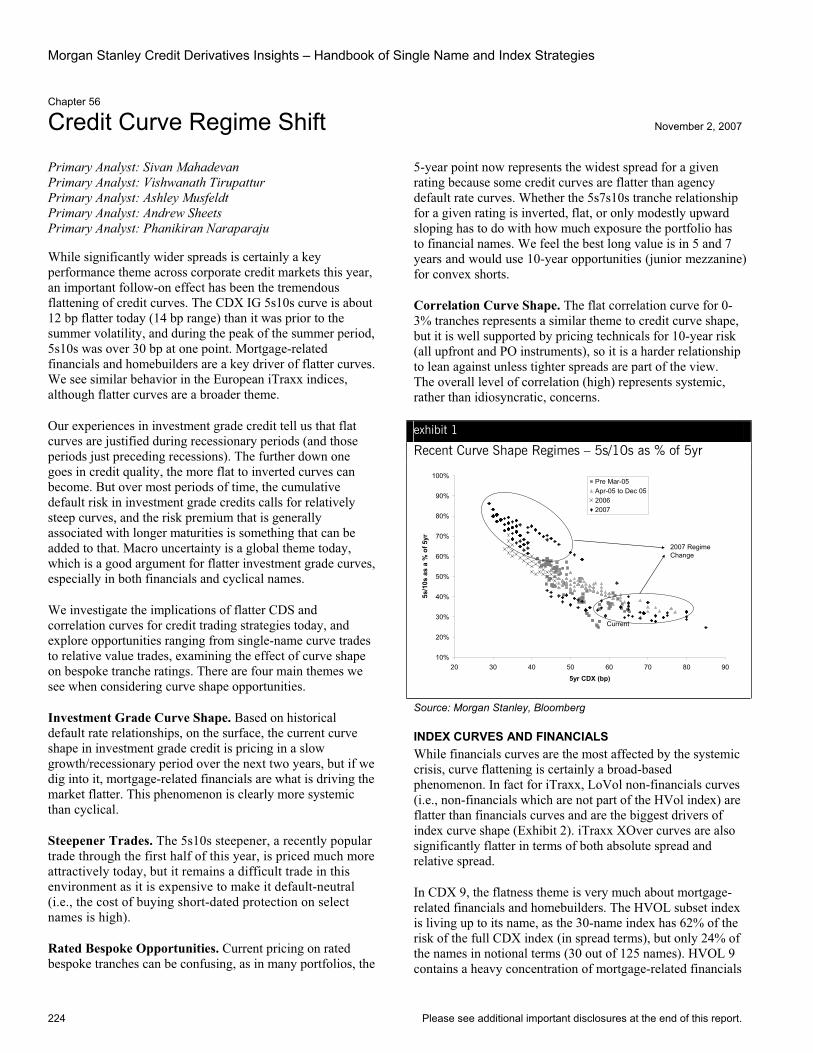
Morgan Stanley Credit Derivatives Insights – Handbook of Single Name and Index Strategies
224 Please see additional important disclosures at the end of this report.
Chapter 56
Credit Curve Regime Shift November 2, 2007
Primary Analyst: Sivan Mahadevan Primary Analyst: Vishwanath Tirupattur Primary Analyst: Ashley Musfeldt Primary Analyst: Andrew Sheets Primary Analyst: Phanikiran Naraparaju
While significantly wider spreads is certainly a key performance theme across corporate credit markets this year, an important follow-on effect has been the tremendous flattening of credit curves. The CDX IG 5s10s curve is about 12 bp flatter today (14 bp range) than it was prior to the summer volatility, and during the peak of the summer period, 5s10s was over 30 bp at one point. Mortgage-related financials and homebuilders are a key driver of flatter curves. We see similar behavior in the European iTraxx indices, although flatter curves are a broader theme.
Our experiences in investment grade credit tell us that flat curves are justified during recessionary periods (and those periods just preceding recessions). The further down one goes in credit quality, the more flat to inverted curves can become. But over most periods of time, the cumulative default risk in investment grade credits calls for relatively steep curves, and the risk premium that is generally associated with longer maturities is something that can be added to that. Macro uncertainty is a global theme today, which is a good argument for flatter investment grade curves, especially in both financials and cyclical names.
We investigate the implications of flatter CDS and correlation curves for credit trading strategies today, and explore opportunities ranging from single-name curve trades to relative value trades, examining the effect of curve shape on bespoke tranche ratings. There are four main themes we see when considering curve shape opportunities.
Investment Grade Curve Shape. Based on historical default rate relationships, on the surface, the current curve shape in investment grade credit is pricing in a slow growth/recessionary period over the next two years, but if we dig into it, mortgage-related financials are what is driving the market flatter. This phenomenon is clearly more systemic than cyclical.
Steepener Trades. The 5s10s steepener, a recently popular trade through the first half of this year, is priced much more attractively today, but it remains a difficult trade in this environment as it is expensive to make it default-neutral (i.e., the cost of buying short-dated protection on select names is high).
Rated Bespoke Opportunities. Current pricing on rated bespoke tranches can be confusing, as in many portfolios, the
5-year point now represents the widest spread for a given rating because some credit curves are flatter than agency default rate curves. Whether the 5s7s10s tranche relationship for a given rating is inverted, flat, or only modestly upward sloping has to do with how much exposure the portfolio has to financial names. We feel the best long value is in 5 and 7 years and would use 10-year opportunities (junior mezzanine) for convex shorts.
Correlation Curve Shape. The flat correlation curve for 0-3% tranches represents a similar theme to credit curve shape, but it is well supported by pricing technicals for 10-year risk (all upfront and PO instruments), so it is a harder relationship to lean against unless tighter spreads are part of the view. The overall level of correlation (high) represents systemic, rather than idiosyncratic, concerns.
exhibit 1
Recent Curve Shape Regimes – 5s/10s as % of 5yr
10%
20%
30%
40%
50%
60%
70%
80%
90%
100%
20 30 40 50 60 70 80 90
5yr CDX (bp)
5s/1
0s a
s a
% o
f 5yr
Pre Mar-05Apr-05 to Dec 0520062007
Current
2007 Regime Change
Source: Morgan Stanley, Bloomberg
INDEX CURVES AND FINANCIALS While financials curves are the most affected by the systemic crisis, curve flattening is certainly a broad-based phenomenon. In fact for iTraxx, LoVol non-financials curves (i.e., non-financials which are not part of the HVol index) are flatter than financials curves and are the biggest drivers of index curve shape (Exhibit 2). iTraxx XOver curves are also significantly flatter in terms of both absolute spread and relative spread.
In CDX 9, the flatness theme is very much about mortgage-related financials and homebuilders. The HVOL subset index is living up to its name, as the 30-name index has 62% of the risk of the full CDX index (in spread terms), but only 24% of the names in notional terms (30 out of 125 names). HVOL 9 contains a heavy concentration of mortgage-related financials
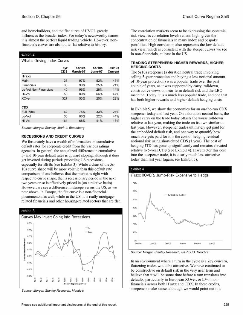
Section D, Chapter 56 Credit Curve Regime Shift
Please see additional important disclosures at the end of this report. 225
and homebuilders, and the flat curve of HVOL greatly influences the broader index. For today’s newsworthy names, it is almost the perfect liquid trading vehicle. However, non-financials curves are also quite flat relative to history.
exhibit 2
What’s Driving Index Curves
5yr CDS
5s/10sMarch-07
5s/10sJune-07
5s/10sCurrent
iTraxx Main 38 97% 52% 45%Financials 35 90% 25% 21%Lo-Vol Non-Financials 40 96% 28% 14%Hi-Vol 53 89% 66% 47%XOver 327 53% 25% 22% CDXFull Index 62 75% 33% 27%Lo-Vol 30 86% 22% 44%Hi-Vol 161 68% 41% 16%
Source: Morgan Stanley, Mark-It, Bloomberg
RECESSIONS AND CREDIT CURVES We fortunately have a wealth of information on cumulative default rates for corporate credit from the various ratings agencies. In general, the annualized difference in cumulative 5- and 10-year default rates is upward sloping, although it does get inverted during periods preceding US recessions, especially for BBBs (see Exhibit 3). While a chart of the 5s-10s curve shape will be more volatile than this default rate comparison, if one believes that the market is right with respect to curve shape, then a recessionary period in the next two years or so is effectively priced in (on a relative basis). However, we see a difference in Europe versus the US, as we note above. In Europe, the flat curve is a non-financial phenomenon, as well, while in the US, it is really mortgage-related financials and other housing-related sectors that are flat.
exhibit 3
Curves May Invert Going into Recessions
-0.3%
-0.2%
-0.1%
0.0%
0.1%
0.2%
0.3%
0.4%
0.5%
1970
1972
1974
1976
1978
1980
1982
1984
1986
1988
1990
1992
1994
1996
Cohort Beginning in Year
Def
ault
Rat
e D
iffer
entia
l
IG
Baa
Source: Morgan Stanley Research, Moody’s
The correlation markets seem to be expressing the systemic risk view, as correlation levels remain high, given the concentration of financials in many index and bespoke portfolios. High correlation also represents the low default risk view, which is consistent with the steeper curves we see in non-financials, at least in the US.
TRADING STEEPENERS: HIGHER REWARDS, HIGHER HEDGING COSTS The 5s10s steepener (a duration neutral trade involving selling 5-year protection and buying a less notional amount of 10-year protection) was a popular trade over the past couple of years, as it was supported by carry, rolldown, constructive views on near-term default risk and the LBO machine. Today, it is a much less popular trade, and one that has both higher rewards and higher default hedging costs.
In Exhibit 5, we show the economics for an on-the-run CDX steepener today and last year. On a duration-neutral basis, the higher carry on the trade today offsets the worse rolldown relative to last year, making the trade on its own similar to last year. However, steepener trades ultimately get paid for the embedded default risk, and one way to quantify how much one gets paid for it is the cost of hedging residual notional risk using short-dated CDS (1 year). The cost of hedging JTD has gone up significantly and remains elevated relative to 5-year CDS (see Exhibit 4). If we factor this cost into the steepener trade, it is clearly much less attractive today than last year (again, see Exhibit 5).
exhibit 4
iTraxx XOVER: Jump-Risk Expensive to Hedge
0%
10%
20%
30%
40%
50%
60%
70%
Dec-04 Jun-05 Dec-05 Jun-06 Dec-06 Jun-07
1yr CDS as % of 5yr
Source: Morgan Stanley Research, S&P LCD, Moody’s
In an environment where a turn in the cycle is a key concern, flattening trades would be attractive. We have continued to be constructive on default risk in the very near term and believe that it will be some time before a turn translates into defaults, particularly in European XOver, or LVol non-financials across both iTraxx and CDX. In these credits, steepeners make sense, although we would point out it is

Morgan Stanley Credit Derivatives Insights – Handbook of Single Name and Index Strategies
226 Please see additional important disclosures at the end of this report.
much less of an index trade, given the presence of financials and homebuilders. We believe this trade is best implemented at the single-name level.
exhibit 5
Trade Mechanics of Steepeners – Then and Now
Oct-06 Oct-07 Hypothetical IG Credit 5 Yr 10 Yr 5 Yr 10 YrSpreads 35 57 60 77Duration 4.5 7.7 4.5 7.6 Oct-06 Oct-07
5s/10s-Steepener Mechanics Duration
Weight Notional
Weight Duration
WeightNotional
WeightLong Risk Leg (Notional MM) 10.0 10.0 10.0 10.0Short Risk Leg (Notional MM) (5.9) (10.0) (5.9) (10.0)JTD Risk Notional 4.1 - 4.1 -JTD Impact (at 40% Recovery)
(MM) (2.5) - (2.5) -JTD Monetization (with 1yr CDS)
(bp) (3.6) - (16.0) -Current Duration - (3.2) - (3.1) Carry (on 10MM) (bp) 2 (22) 15 (16)Rolldown (on 10MM) (bp) 17 9 4 (1)Carry + Rolldown (bp) 19 (12) 19 (18)Carry + Rolldown + JTD (bp) 15 39 3 39 After 5yrs Notional (MM) (5.9) (10.0) (5.9) (10.0)Spread (bp) (57) (57) (77) (77)PV of Unwind (bp) 57 98 43 73
Source: Morgan Stanley
STEEPENERS AND CONVEXITY Current market turmoil has made investors acutely attuned to direct or indirect convexity exposures. We have had various discussions on whether convexity is inherent in curve positions, and our sense is that the answer varies depending on the regime. At tight spread levels, such as those that prevailed during 2005-06, steepeners are positively convex. Any incremental spread widening leads to steeper curves, as spreads are still too tight and default risk perception is still limited. On the other hand, tighter spread levels result in spread compression at the short end first, leading to a bullish flattening of credit curves. However, in the current environment, the impact is less clear, and a steepener can be viewed as a negatively convex trade. Further widening from current spread levels would be driven by increased concern about default risk and could lead to further flattening of credit curves.
RATED BESPOKES – IMPLICATIONS OF CURVE ENVIRONMENTFor rated bespoke investors, there can be both confusion and opportunity in this curve environment. With a somewhat
justified flat credit spread curve, especially in financially heavy portfolios, the task at hand is forming views on where the value is along both the ratings and maturity spectrum. A portfolio that takes advantage of flat financials will actually be more likely to offer a higher spread for a given rating at the five-year point versus the 7- or 10-year point. This may seem non-intuitive, but as long as credit curves are flatter than the long-run rating agency default probability curves, it is both possible and very observable in the market.
However, whether the rated bespoke curve is inverted, flat, or only moderately upward sloping, the bottom line is that we see much value in 5- and 7-year bespoke tranches from the long side, as we are attracted by lower durations, the time decay associated with a continued low default environment, and the potential for the curves to re-steepen if systemic risks are reduced. We would focus short ideas (where we have a preference for junior mezzanine tranches) on the 10-year part of the curve.
CORRELATION CURVES – HARD TO LEAN AGAINST FLATNESS Another important curve-related theme is the flatness that we see in correlation curves for the standard index equity tranches. Simply put, despite the fact that credit curves are flat from a spread perspective, equity tranche investors are assigning little to no risk premium in correlation terms for 7- and 10-year equity risk versus 5-year. The reason is very technical, in our view, as wide spreads push all-upfront prices on the 10-year 0-3% tranche to the 80% level, which is attractive from an upside/downside skew perspective. Furthermore, PO flows are very price driven (IG 9 10-year POs are in the 6% range now; IG 8 is in the 5% range). As such, a “normalization” of the equity correlation curve can really only happen with meaningfully tighter spreads.
CONCLUSION – REGIME SHIFT Today’s very flat credit curves do not present an obvious opportunity to lean against with steepening trades. In fact, we would argue that recent performance and concerns in the financial sector are worse than they were in the summer, when we felt more comfortable leaning against very flat curves.
Yet, markets are not efficient, and there are opportunities to lean against flat curves in non-financial credits that are not directly exposed to the housing markets. These opportunities require either taking near-term default risk, or hedging it with short-dated protection. On the bespoke tranche side, we think the regime shift is an invitation to move down the maturity curve and focus on 5- and 7-year opportunities from the long side, and 10-years from the short side.

Section E
Options and Embedded Options
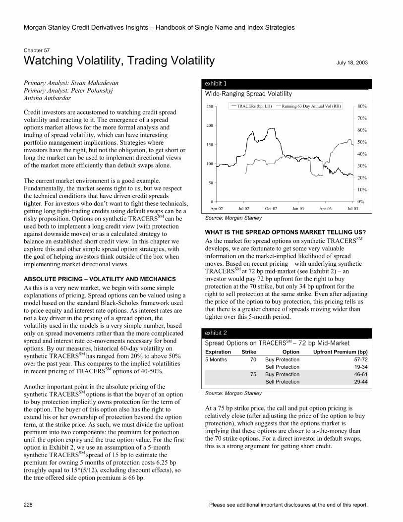
Morgan Stanley Credit Derivatives Insights – Handbook of Single Name and Index Strategies
228 Please see additional important disclosures at the end of this report.
Chapter 57
Watching Volatility, Trading Volatility July 18, 2003
Primary Analyst: Sivan Mahadevan Primary Analyst: Peter Polanskyj Anisha Ambardar
Credit investors are accustomed to watching credit spread volatility and reacting to it. The emergence of a spread options market allows for the more formal analysis and trading of spread volatility, which can have interesting portfolio management implications. Strategies where investors have the right, but not the obligation, to get short or long the market can be used to implement directional views of the market more efficiently than default swaps alone.
The current market environment is a good example. Fundamentally, the market seems tight to us, but we respect the technical conditions that have driven credit spreads tighter. For investors who don’t want to fight these technicals, getting long tight-trading credits using default swaps can be a risky proposition. Options on synthetic TRACERSSM can be used both to implement a long credit view (with protection against downside moves) or as a calculated strategy to balance an established short credit view. In this chapter we explore this and other simple spread option strategies, with the goal of helping investors think outside of the box when implementing market directional views.
ABSOLUTE PRICING – VOLATILITY AND MECHANICS As this is a very new market, we begin with some simple explanations of pricing. Spread options can be valued using a model based on the standard Black-Scholes framework used to price equity and interest rate options. As interest rates are not a key driver in the pricing of a spread option, the volatility used in the models is a very simple number, based only on spread movements rather than the more complicated spread and interest rate co-movements necessary for bond options. By our measures, historical 60-day volatility on synthetic TRACERSSM has ranged from 20% to above 50% over the past year. This compares to the implied volatilities in recent pricing of TRACERSSM options of 40-50%.
Another important point in the absolute pricing of the synthetic TRACERSSM options is that the buyer of an option to buy protection implicitly owns protection for the term of the option. The buyer of this option also has the right to extend his or her ownership of protection beyond the option term, at the strike price. As such, we must divide the upfront premium into two components: the premium for protection until the option expiry and the true option value. For the first option in Exhibit 2, we use an assumption of a 5-month synthetic TRACERSSM spread of 15 bp to estimate the premium for owning 5 months of protection costs 6.25 bp (roughly equal to 15*(5/12), excluding discount effects), so the true offered side option premium is 66 bp.
exhibit 1
Wide-Ranging Spread Volatility
0
50
100
150
200
250
Apr-02 Jul-02 Oct-02 Jan-03 Apr-03 Jul-030%
10%
20%
30%
40%
50%
60%
70%
80%TRACERs (bp, LH) Running 63 Day Annual Vol (RH)
Source: Morgan Stanley
WHAT IS THE SPREAD OPTIONS MARKET TELLING US? As the market for spread options on synthetic TRACERSSM
develops, we are fortunate to get some very valuable information on the market-implied likelihood of spread moves. Based on recent pricing – with underlying synthetic TRACERSSM at 72 bp mid-market (see Exhibit 2) – an investor would pay 72 bp upfront for the right to buy protection at the 70 strike, but only 34 bp upfront for the right to sell protection at the same strike. Even after adjusting the price of the option to buy protection, this pricing tells us that there is a greater chance of spreads moving wider than tighter over this 5-month period.
exhibit 2
Spread Options on TRACERSSM – 72 bp Mid-Market Expiration Strike Option Upfront Premium (bp)5 Months 70 Buy Protection 57-72 Sell Protection 19-34
75 Buy Protection 46-61Sell Protection 29-44
Source: Morgan Stanley
At a 75 bp strike price, the call and put option pricing is relatively close (after adjusting the price of the option to buy protection), which suggests that the options market is implying that these options are closer to at-the-money than the 70 strike options. For a direct investor in default swaps, this is a strong argument for getting short credit.
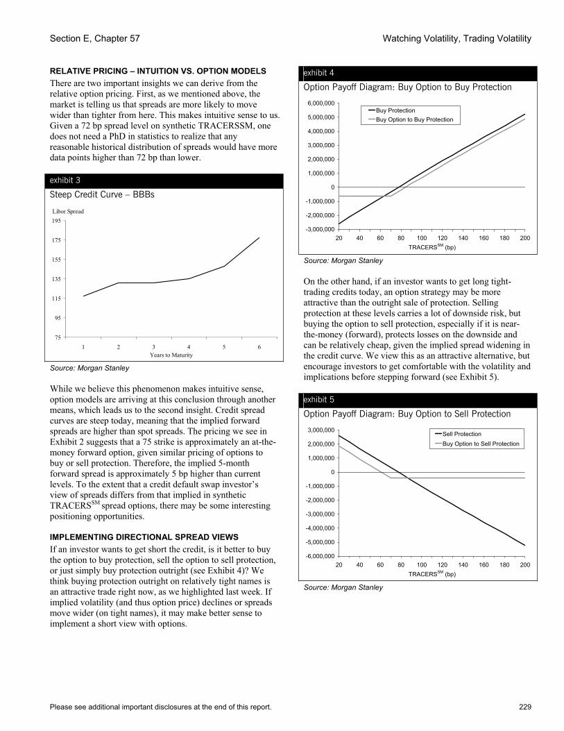
Section E, Chapter 57 Watching Volatility, Trading Volatility
Please see additional important disclosures at the end of this report. 229
RELATIVE PRICING – INTUITION VS. OPTION MODELS There are two important insights we can derive from the relative option pricing. First, as we mentioned above, the market is telling us that spreads are more likely to move wider than tighter from here. This makes intuitive sense to us. Given a 72 bp spread level on synthetic TRACERSSM, one does not need a PhD in statistics to realize that any reasonable historical distribution of spreads would have more data points higher than 72 bp than lower.
exhibit 3
Steep Credit Curve – BBBs
Libor Spread
75
95
115
135
155
175
195
1 2 3 4 5 6Years to Maturity
Source: Morgan Stanley
While we believe this phenomenon makes intuitive sense, option models are arriving at this conclusion through another means, which leads us to the second insight. Credit spread curves are steep today, meaning that the implied forward spreads are higher than spot spreads. The pricing we see in Exhibit 2 suggests that a 75 strike is approximately an at-the-money forward option, given similar pricing of options to buy or sell protection. Therefore, the implied 5-month forward spread is approximately 5 bp higher than current levels. To the extent that a credit default swap investor’s view of spreads differs from that implied in synthetic TRACERSSM spread options, there may be some interesting positioning opportunities.
IMPLEMENTING DIRECTIONAL SPREAD VIEWS If an investor wants to get short the credit, is it better to buy the option to buy protection, sell the option to sell protection, or just simply buy protection outright (see Exhibit 4)? We think buying protection outright on relatively tight names is an attractive trade right now, as we highlighted last week. If implied volatility (and thus option price) declines or spreads move wider (on tight names), it may make better sense to implement a short view with options.
exhibit 4
Option Payoff Diagram: Buy Option to Buy Protection
-3,000,000
-2,000,000
-1,000,000
0
1,000,000
2,000,000
3,000,000
4,000,000
5,000,000
6,000,000
20 40 60 80 100 120 140 160 180 200TRACERSSM (bp)
Buy ProtectionBuy Option to Buy Protection
Source: Morgan Stanley
On the other hand, if an investor wants to get long tight-trading credits today, an option strategy may be more attractive than the outright sale of protection. Selling protection at these levels carries a lot of downside risk, but buying the option to sell protection, especially if it is near-the-money (forward), protects losses on the downside and can be relatively cheap, given the implied spread widening in the credit curve. We view this as an attractive alternative, but encourage investors to get comfortable with the volatility and implications before stepping forward (see Exhibit 5).
exhibit 5
Option Payoff Diagram: Buy Option to Sell Protection
-6,000,000
-5,000,000
-4,000,000
-3,000,000
-2,000,000
-1,000,000
0
1,000,000
2,000,000
3,000,000
20 40 60 80 100 120 140 160 180 200TRACERSSM (bp)
Sell ProtectionBuy Option to Sell Protection
Source: Morgan Stanley

Morgan Stanley Credit Derivatives Insights – Handbook of Single Name and Index Strategies
230 Please see additional important disclosures at the end of this report.
IMPLEMENTING VIEWS ON VOLATILITY Given the relatively high level of implied volatility today as compared to actual volatility over the past year (a rather volatile year for spreads), a relevant application of options comes from the view that we could live in a low volatility world going forward, and any incremental implied volatility should be monetized now to add yield to a portfolio. For investors with this view, implied synthetic TRACERSSM volatility levels are attractive. For example, selling the 5-month option to buy protection at 75 bp today generates 46 bp upfront, or the equivalent of 110 bp running. Assuming the option is exercised, the seller will generate a forward spread of 75 on TRACERSSM
plus 110 bp in the initial option period versus generating 72 bp by selling protection today. The key risk in this position is a spread tightening beyond the approximate 4 bp of buffer created by the monetization of volatility.
Taking the low volatility view one step further, investors could combine this position with the sale of an option to sell protection struck at 70 (creating a spread strangle), thereby generating 65 bp upfront or the equivalent of approximately 156 bp running, while bearing the risk of spreads moving outside the 70-75 range.
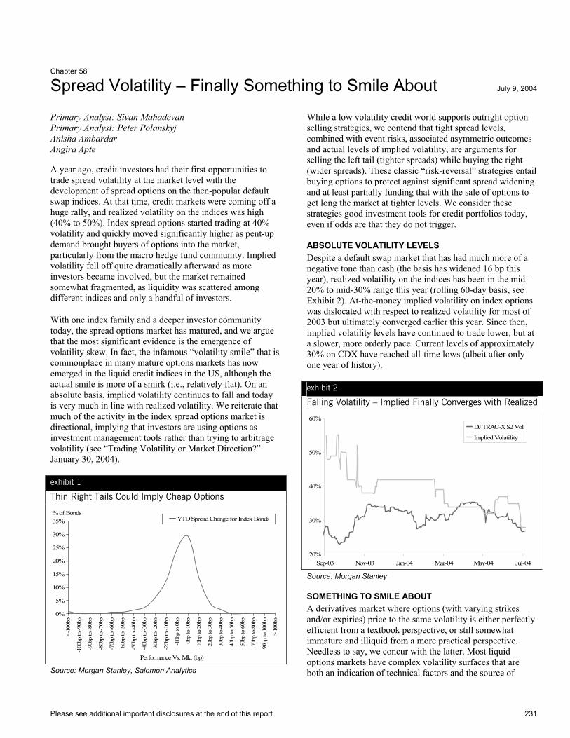
Please see additional important disclosures at the end of this report. 231
Chapter 58
Spread Volatility – Finally Something to Smile About July 9, 2004
Primary Analyst: Sivan Mahadevan Primary Analyst: Peter Polanskyj Anisha Ambardar Angira Apte
A year ago, credit investors had their first opportunities to trade spread volatility at the market level with the development of spread options on the then-popular default swap indices. At that time, credit markets were coming off a huge rally, and realized volatility on the indices was high (40% to 50%). Index spread options started trading at 40% volatility and quickly moved significantly higher as pent-up demand brought buyers of options into the market, particularly from the macro hedge fund community. Implied volatility fell off quite dramatically afterward as more investors became involved, but the market remained somewhat fragmented, as liquidity was scattered among different indices and only a handful of investors.
With one index family and a deeper investor community today, the spread options market has matured, and we argue that the most significant evidence is the emergence of volatility skew. In fact, the infamous “volatility smile” that is commonplace in many mature options markets has now emerged in the liquid credit indices in the US, although the actual smile is more of a smirk (i.e., relatively flat). On an absolute basis, implied volatility continues to fall and today is very much in line with realized volatility. We reiterate that much of the activity in the index spread options market is directional, implying that investors are using options as investment management tools rather than trying to arbitrage volatility (see “Trading Volatility or Market Direction?” January 30, 2004).
exhibit 1
Thin Right Tails Could Imply Cheap Options
% of Bonds
0%
5%
10%
15%
20%
25%
30%
35%
> -1
00bp
-100
bp to
-90b
p
-90b
p to
-80b
p
-80b
p to
-70b
p
-70b
p to
-60b
p
-60b
p to
-50b
p
-50b
p to
-40b
p
-40b
p to
-30b
p
-30b
p to
-20b
p
-20b
p to
-10b
p
-10b
p to
0bp
0bp
to 1
0bp
10bp
to 2
0bp
20bp
to 3
0bp
30bp
to 4
0bp
40bp
to 5
0bp
50bp
to 6
0bp
70bp
to 8
0bp
90bp
to 1
00bp
> 10
0bp
Performance Vs. Mkt (bp)
YTD Spread Change for Index Bonds
Source: Morgan Stanley, Salomon Analytics
While a low volatility credit world supports outright option selling strategies, we contend that tight spread levels, combined with event risks, associated asymmetric outcomes and actual levels of implied volatility, are arguments for selling the left tail (tighter spreads) while buying the right (wider spreads). These classic “risk-reversal” strategies entail buying options to protect against significant spread widening and at least partially funding that with the sale of options to get long the market at tighter levels. We consider these strategies good investment tools for credit portfolios today, even if odds are that they do not trigger.
ABSOLUTE VOLATILITY LEVELS Despite a default swap market that has had much more of a negative tone than cash (the basis has widened 16 bp this year), realized volatility on the indices has been in the mid-20% to mid-30% range this year (rolling 60-day basis, see Exhibit 2). At-the-money implied volatility on index options was dislocated with respect to realized volatility for most of 2003 but ultimately converged earlier this year. Since then, implied volatility levels have continued to trade lower, but at a slower, more orderly pace. Current levels of approximately 30% on CDX have reached all-time lows (albeit after only one year of history).
exhibit 2
Falling Volatility – Implied Finally Converges with Realized
20%
30%
40%
50%
60%
Sep-03 Nov-03 Jan-04 Mar-04 May-04 Jul-04
DJ TRAC-X S2 Vol
Implied Volatility
Source: Morgan Stanley
SOMETHING TO SMILE ABOUT A derivatives market where options (with varying strikes and/or expiries) price to the same volatility is either perfectly efficient from a textbook perspective, or still somewhat immature and illiquid from a more practical perspective. Needless to say, we concur with the latter. Most liquid options markets have complex volatility surfaces that are both an indication of technical factors and the source of
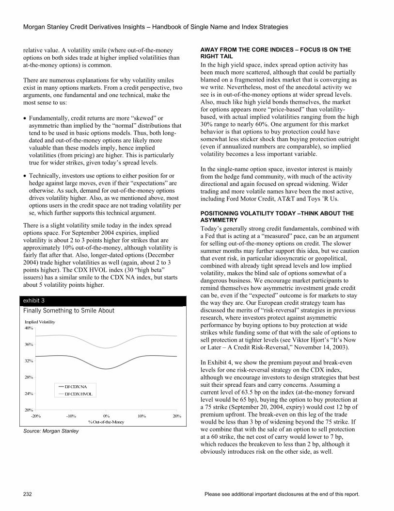
Morgan Stanley Credit Derivatives Insights – Handbook of Single Name and Index Strategies
232 Please see additional important disclosures at the end of this report.
relative value. A volatility smile (where out-of-the-money options on both sides trade at higher implied volatilities than at-the-money options) is common.
There are numerous explanations for why volatility smiles exist in many options markets. From a credit perspective, two arguments, one fundamental and one technical, make the most sense to us:
• Fundamentally, credit returns are more “skewed” or asymmetric than implied by the “normal” distributions that tend to be used in basic options models. Thus, both long-dated and out-of-the-money options are likely more valuable than these models imply, hence implied volatilities (from pricing) are higher. This is particularly true for wider strikes, given today’s spread levels.
• Technically, investors use options to either position for or hedge against large moves, even if their “expectations” are otherwise. As such, demand for out-of-the-money options drives volatility higher. Also, as we mentioned above, most options users in the credit space are not trading volatility per se, which further supports this technical argument.
There is a slight volatility smile today in the index spread options space. For September 2004 expiries, implied volatility is about 2 to 3 points higher for strikes that are approximately 10% out-of-the-money, although volatility is fairly flat after that. Also, longer-dated options (December 2004) trade higher volatilities as well (again, about 2 to 3 points higher). The CDX HVOL index (30 “high beta” issuers) has a similar smile to the CDX NA index, but starts about 5 volatility points higher.
exhibit 3
Finally Something to Smile About
Implied Volatility
20%
24%
28%
32%
36%
40%
-20% -10% 0% 10% 20%% Out-of-the-Money
DJ CDX NA
DJ CDX HVOL
Source: Morgan Stanley
AWAY FROM THE CORE INDICES – FOCUS IS ON THE RIGHT TAIL In the high yield space, index spread option activity has been much more scattered, although that could be partially blamed on a fragmented index market that is converging as we write. Nevertheless, most of the anecdotal activity we see is in out-of-the-money options at wider spread levels. Also, much like high yield bonds themselves, the market for options appears more “price-based” than volatility-based, with actual implied volatilities ranging from the high 30% range to nearly 60%. One argument for this market behavior is that options to buy protection could have somewhat less sticker shock than buying protection outright (even if annualized numbers are comparable), so implied volatility becomes a less important variable.
In the single-name option space, investor interest is mainly from the hedge fund community, with much of the activity directional and again focused on spread widening. Wider trading and more volatile names have been the most active, including Ford Motor Credit, AT&T and Toys ’R Us.
POSITIONING VOLATILITY TODAY –THINK ABOUT THE ASYMMETRY Today’s generally strong credit fundamentals, combined with a Fed that is acting at a “measured” pace, can be an argument for selling out-of-the-money options on credit. The slower summer months may further support this idea, but we caution that event risk, in particular idiosyncratic or geopolitical, combined with already tight spread levels and low implied volatility, makes the blind sale of options somewhat of a dangerous business. We encourage market participants to remind themselves how asymmetric investment grade credit can be, even if the “expected” outcome is for markets to stay the way they are. Our European credit strategy team has discussed the merits of “risk-reversal” strategies in previous research, where investors protect against asymmetric performance by buying options to buy protection at wide strikes while funding some of that with the sale of options to sell protection at tighter levels (see Viktor Hjort’s “It’s Now or Later – A Credit Risk-Reversal,” November 14, 2003).
In Exhibit 4, we show the premium payout and break-even levels for one risk-reversal strategy on the CDX index, although we encourage investors to design strategies that best suit their spread fears and carry concerns. Assuming a current level of 63.5 bp on the index (at-the-money forward level would be 65 bp), buying the option to buy protection at a 75 strike (September 20, 2004, expiry) would cost 12 bp of premium upfront. The break-even on this leg of the trade would be less than 3 bp of widening beyond the 75 strike. If we combine that with the sale of an option to sell protection at a 60 strike, the net cost of carry would lower to 7 bp, which reduces the breakeven to less than 2 bp, although it obviously introduces risk on the other side, as well.

Section E, Chapter 58 Spread Volatility – Finally Something to Smile About
Please see additional important disclosures at the end of this report. 233
exhibit 4
Sell the Option to Sell, Buy the Option to Buy (CDX at 63.5 bp) Option Strike Expiry Premium BreakevenBuy Buyer 75 Sep 04 0.12% < 3 bpSell Seller 60 Sep 04 0.05%Net 0.07%
Source: Morgan Stanley
Strategies like this make sense for investors who are running underlying credit portfolios that are either overweight with respect to their benchmarks, or higher beta in nature. For investors who prefer long-dated options, or much further out-
of-the-money strikes, we encourage buying protection on index tranches (such as 7-10% or 10-15%). The pricing and convexity of such tranches makes them behave like options in significantly wider markets, as we have addressed in previous research (see “Correlation Conversations, Convexity Ideas,” August 1, 2003).
Finally, as an aside, one of the most confusing aspects of the index options market is the terminology. We like to think of it as simply buying or selling options to buy or sell protection. Options to buy protection are also called buyer options, payer options or sometimes puts. Similarly, options to sell protection are also called seller options, receiver options or sometimes calls.

Morgan Stanley Credit Derivatives Insights – Handbook of Single Name and Index Strategies
234 Please see additional important disclosures at the end of this report.
Chapter 59
Selling Tomorrow’s Tightening Today May 7, 2004
Primary Analyst: Sivan Mahadevan Primary Analyst: Peter Polanskyj Anisha Ambardar Angira Apte
We argued several months ago that the use of single-name options, undoubtedly the most basic of textbook derivatives strategies, would take some time to gain acceptance in the credit markets. To investors outside of our markets, it may seem a bit odd that a simple call or put option on a company’s credit is a much less popular derivative instrument than, say, a 7-10% tranche on a 125-name portfolio that requires a sophisticated correlation model to value properly. However, the popularity of correlation instruments stems from the long history of the CDO market and all the reasons investors continue to use it. Basic options strategies, on the other hand, are very new to credit investors, and will continue to take some time to garner broad acceptance.
The cancelable default swaps segment of the credit options space may seem the most intuitive to many credit investors, given the analogies one can make with callable bonds. In such a swap, the buyer of protection has the right to cancel the swap (after some non-call period), and the seller of protection gets paid additional premium to be “short” this option. The natural buyers of this protection include those who need to be short credit as a matter of business, but fear tightening spreads (bank loan hedgers), as well as those who hedge long credit positions with uncertain maturities (e.g., banks, convertible bond users, high yield investors). The natural sellers of cancelable protection include those who need to be long credit as a matter of business but do not expect a significant tightening of spreads. In a sense, selling cancelable protection is a way of forming a neutral-to-bearish view on credit spreads in the future, from the long side.
THE MECHANICS OF A CANCELABLE DEFAULT SWAP A cancelable default swap (also known as a callable default swap) is simply a credit default swap (with standard credit events) where the buyer of protection has the right to cancel the protection after a non-call period. Such a feature is not unique to credit derivatives; it exists in the interest rate derivatives world, as well. From the seller of protection’s perspective, one can think of a cancelable default swap as a covered call strategy, similar to a callable bond, where the seller of protection is “short” a call option that is not exercisable until the non-call period ends. The performance of selling callable protection has the typical hockey stick shape associated with instruments with embedded options (when the non-call period is over – see Exhibit 1).
exhibit 1
Cancelable vs. Bullet CDS – The Hockey Stick
Total Return
-3.0%
-2.0%
-1.0%
0.0%
1.0%
2.0%
3.0%
4.0%
5.0%
27
34
40
47
54
60
67
74
80 87 94 101
107
114
121
127
134
Bullet CDS Premium
Bullet
Cancelable
Source: Morgan Stanley
Unlike a callable bond, there is no explicit strike price in a cancelable default swap. Protection buyers will cancel the protection when they no longer need it. The economic incentive to do this is when spreads are tighter than the par spread on the swap, but there could be other reasons why a buyer chooses to cancel protection – for example, when an associated long credit position prepays or gets called away.
In a pure options sense, the option embedded in a cancelable default swap is less valuable than the option in a callable bond, at least based on historical volatility differences. For example, the volatility of investment grade spread movements is less than one-third the volatility of interest rate movements over the past 2 ½ years (35 bp versus 118 bp).
THE MARKET, VALUATION AND SENSITIVITY Though market activity is limited for cancelable default swaps, we do have some pricing information from which we can better understand both valuation and sensitivity. For the credits in Exhibit 2 (ranging from 25 bp to 255 bp bid side), cancelable protection trades on average 19% wider, reflecting the value of the embedded option (and any additional liquidity premium).
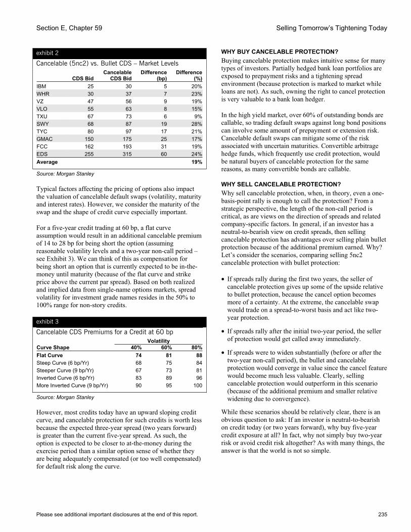
Section E, Chapter 59 Selling Tomorrow’s Tightening Today
Please see additional important disclosures at the end of this report. 235
exhibit 2
Cancelable (5nc2) vs. Bullet CDS – Market Levels
CDS Bid Cancelable
CDS Bid Difference
(bp)Difference
(%)IBM 25 30 5 20%WHR 30 37 7 23%VZ 47 56 9 19%VLO 55 63 8 15%TXU 67 73 6 9%SWY 68 87 19 28%TYC 80 97 17 21%GMAC 150 175 25 17%FCC 162 193 31 19%EDS 255 315 60 24%Average 19%
Source: Morgan Stanley
Typical factors affecting the pricing of options also impact the valuation of cancelable default swaps (volatility, maturity and interest rates). However, we consider the maturity of the swap and the shape of credit curve especially important.
For a five-year credit trading at 60 bp, a flat curve assumption would result in an additional cancelable premium of 14 to 28 bp for being short the option (assuming reasonable volatility levels and a two-year non-call period – see Exhibit 3). We can think of this as compensation for being short an option that is currently expected to be in-the-money until maturity (because of the flat curve and strike price above the current par spread). Based on both realized and implied data from single-name options markets, spread volatility for investment grade names resides in the 50% to 100% range for non-story credits.
exhibit 3
Cancelable CDS Premiums for a Credit at 60 bp Volatility Curve Shape 40% 60% 80%Flat Curve 74 81 88Steep Curve (6 bp/Yr) 68 75 84Steeper Curve (9 bp/Yr) 67 73 81Inverted Curve (6 bp/Yr) 83 89 96More Inverted Curve (9 bp/Yr) 90 95 100
Source: Morgan Stanley
However, most credits today have an upward sloping credit curve, and cancelable protection for such credits is worth less because the expected three-year spread (two years forward) is greater than the current five-year spread. As such, the option is expected to be closer to at-the-money during the exercise period than a similar option sense of whether they are being adequately compensated (or too well compensated) for default risk along the curve.
WHY BUY CANCELABLE PROTECTION? Buying cancelable protection makes intuitive sense for many types of investors. Partially hedged bank loan portfolios are exposed to prepayment risks and a tightening spread environment (because protection is marked to market while loans are not). As such, owning the right to cancel protection is very valuable to a bank loan hedger.
In the high yield market, over 60% of outstanding bonds are callable, so trading default swaps against long bond positions can involve some amount of prepayment or extension risk. Cancelable default swaps can mitigate some of the risk associated with uncertain maturities. Convertible arbitrage hedge funds, which frequently use credit protection, would be natural buyers of cancelable protection for the same reasons, as many convertible bonds are callable.
WHY SELL CANCELABLE PROTECTION? Why sell cancelable protection, when, in theory, even a one-basis-point rally is enough to call the protection? From a strategic perspective, the length of the non-call period is critical, as are views on the direction of spreads and related company-specific factors. In general, if an investor has a neutral-to-bearish view on credit spreads, then selling cancelable protection has advantages over selling plain bullet protection because of the additional premium earned. Why? Let’s consider the scenarios, comparing selling 5nc2 cancelable protection with bullet protection:
• If spreads rally during the first two years, the seller of cancelable protection gives up some of the upside relative to bullet protection, because the cancel option becomes more of a certainty. At the extreme, the cancelable swap would trade on a spread-to-worst basis and act like two-year protection.
• If spreads rally after the initial two-year period, the seller of protection would get called away immediately.
• If spreads were to widen substantially (before or after the two-year non-call period), the bullet and cancelable protection would converge in value since the cancel feature would become much less valuable. Clearly, selling cancelable protection would outperform in this scenario (because of the additional premium and smaller relative widening due to convergence).
While these scenarios should be relatively clear, there is an obvious question to ask: If an investor is neutral-to-bearish on credit today (or two years forward), why buy five-year credit exposure at all? In fact, why not simply buy two-year risk or avoid credit risk altogether? As with many things, the answer is that the world is not so simple.

Morgan Stanley Credit Derivatives Insights – Handbook of Single Name and Index Strategies
236 Please see additional important disclosures at the end of this report.
LONG CREDIT AS A MATTER OF BUSINESS We live in a world where many investors need to be long credit as a matter of business. Insurance companies and benchmarked money managers are the natural examples. Feeling negative on an asset class is not always a good enough reason to get out completely. Selling cancelable protection is a way of implementing an underweight position in credit today (because spread durations are lower), and getting paid in yield terms to do so (because premiums are higher). But even more powerful, selling cancelable protection is a way of playing credit cycles, because investors are effectively selling away the scenario where spreads tighten at some point in the future. The motivation behind this strategy would be fear of increased corporate leverage in the future as the US economy continues to expand, or simply a turn in the cycle at that point.
Of course, buying two-year risk instead of five-year risk is another way to express forward fears of increased leverage or turning cycles. Yet, given today’s steep credit curve (in the short end), the additional premium of 5nc2 protection over two-year protection is substantial. One has to be extremely negative on credit over the next two years to make the premium give-up worthwhile.
SELLING TOMORROW’S TIGHTENING TODAY Away from the structural reasons supporting the buying and selling of cancelable protection, we favor the idea of positioning for a neutral-to-weaker credit environment later on in this economic expansionary period, given the cyclical nature of credit and corporate leverage. Although there are many ways to express these views using long/short strategies, selling cancelable protection is a natural way to implement them from the long side. However, we caution that this nascent market still needs to grow from both a breadth and depth perspective.

Please see additional important disclosures at the end of this report. 237
Chapter 60
Understanding Corporate Bond Options –Valuation Issues and Portfolio Applications June 11, 2003
Primary Analyst: Sivan Mahadevan Primary Analyst: Peter Polanskyj
INTRODUCTIONOptions on corporate bonds, the right to buy or sell a bond at the strike price during a specific period, were among the earliest credit derivative instruments in the credit markets. Most outstanding corporate bond options are embedded in corporate bonds and are thus implicitly held by either bond issuers (for call options) or bond investors (for put options). As the market for separately traded corporate bond options develops, we focus our research efforts on understanding their investment characteristics, application in credit portfolios and valuation.
The corporate bond options that trade in the secondary market are typically sourced from simple structured credit transactions in which investors, issuers or underwriters write options on bonds to create desired investment characteristics or additional yield. The options are then redistributed and traded in the secondary market. Examples of structured credit transactions that result in new options written include:
• Repackagings of corporate bonds into trusts, in which end investors write call options for additional yield and reductions in average life
• Repackagings of putable corporate bonds into bullet securities, in which the investor would sell a call option with an exercise date equal to the exercise date of the embedded put option
• Writing of at-the-money options by investors who want to protect gains made in bullet securities prior to a rising rate environment (writing covered calls)
It is important to note a few points with respect to outstanding options. First, while corporate issuers are the largest holders of call options on corporate bonds, they typically do not redistribute this risk, although in theory they could. Issuers who hold call options may not exercise them whenever it makes economic sense (i.e., they may not act as rational market participants in the academic sense). The reasons for this behavior may include corporate capital structure issues, funding costs and liquidity in the primary markets. End investors who hold options will likely act more rationally, in the academic sense.
In this chapter we first explore the investment characteristics of corporate bond options, discussing both portfolio applications and trading strategies. We then propose a valuation framework based on traditional swaption market practices but taking into consideration differences in volatility and the likelihood of default. We conclude with some discussion of practical issues for investors that may affect how investors can incorporate these instruments into portfolios to help achieve investment objectives.
Investment Characteristics, Portfolio Applications and Trading Strategies Since callable corporate bonds are a common instrument in the credit markets (5% of index-eligible investment grade corporate bonds are callable, representing $55 billion of debt), we begin our discussion of corporate bond options with a comparison of the price sensitivity of a bullet bond with that of a callable bond with the same terms. In Exhibit 1 we show the price changes relative to yield changes for a bullet bond with a 30-year maturity, along with those of a similar instrument that is callable after three years. The holder of a callable bond (who has written a call to the issuer) effectively gives up the positive performance of the highlighted region when compared to the performance of the bullet security.
exhibit 1
The Call Option Region
Price
60
80
100
120
140
160
180
200
1.75
2.25
2.75
3.25
3.75
4.25
4.75
5.25
5.75
5.95
6.15
6.35
6.55
6.75
6.95
7.15
7.35
7.55
7.75
7.95
Yield
30 Yr Bullet 30 Yr NC 3
Option Value
Source: Morgan Stanley
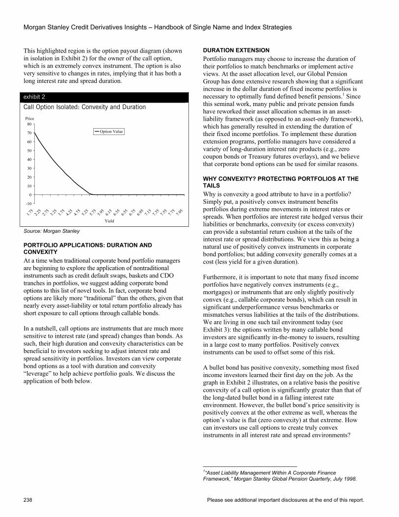
Morgan Stanley Credit Derivatives Insights – Handbook of Single Name and Index Strategies
238 Please see additional important disclosures at the end of this report.
This highlighted region is the option payout diagram (shown in isolation in Exhibit 2) for the owner of the call option, which is an extremely convex instrument. The option is also very sensitive to changes in rates, implying that it has both a long interest rate and spread duration.
exhibit 2
Call Option Isolated: Convexity and Duration
Price
-10
0
10
20
30
40
50
60
70
80
1.75
2.25
2.75
3.25
3.75
4.25
4.75
5.25
5.75
5.95
6.15
6.35
6.55
6.75
6.95
7.15
7.35
7.55
7.75
7.95
Yield
Option Value
Source: Morgan Stanley
PORTFOLIO APPLICATIONS: DURATION AND CONVEXITYAt a time when traditional corporate bond portfolio managers are beginning to explore the application of nontraditional instruments such as credit default swaps, baskets and CDO tranches in portfolios, we suggest adding corporate bond options to this list of novel tools. In fact, corporate bond options are likely more “traditional” than the others, given that nearly every asset-liability or total return portfolio already has short exposure to call options through callable bonds.
In a nutshell, call options are instruments that are much more sensitive to interest rate (and spread) changes than bonds. As such, their high duration and convexity characteristics can be beneficial to investors seeking to adjust interest rate and spread sensitivity in portfolios. Investors can view corporate bond options as a tool with duration and convexity “leverage” to help achieve portfolio goals. We discuss the application of both below.
DURATION EXTENSION Portfolio managers may choose to increase the duration of their portfolios to match benchmarks or implement active views. At the asset allocation level, our Global Pension Group has done extensive research showing that a significant increase in the dollar duration of fixed income portfolios is necessary to optimally fund defined benefit pensions.1 Since this seminal work, many public and private pension funds have reworked their asset allocation schemas in an asset-liability framework (as opposed to an asset-only framework), which has generally resulted in extending the duration of their fixed income portfolios. To implement these duration extension programs, portfolio managers have considered a variety of long-duration interest rate products (e.g., zero coupon bonds or Treasury futures overlays), and we believe that corporate bond options can be used for similar reasons.
WHY CONVEXITY? PROTECTING PORTFOLIOS AT THE TAILS Why is convexity a good attribute to have in a portfolio? Simply put, a positively convex instrument benefits portfolios during extreme movements in interest rates or spreads. When portfolios are interest rate hedged versus their liabilities or benchmarks, convexity (or excess convexity) can provide a substantial return cushion at the tails of the interest rate or spread distributions. We view this as being a natural use of positively convex instruments in corporate bond portfolios; but adding convexity generally comes at a cost (less yield for a given duration).
Furthermore, it is important to note that many fixed income portfolios have negatively convex instruments (e.g., mortgages) or instruments that are only slightly positively convex (e.g., callable corporate bonds), which can result in significant underperformance versus benchmarks or mismatches versus liabilities at the tails of the distributions. We are living in one such tail environment today (see Exhibit 3): the options written by many callable bond investors are significantly in-the-money to issuers, resulting in a large cost to many portfolios. Positively convex instruments can be used to offset some of this risk.
A bullet bond has positive convexity, something most fixed income investors learned their first day on the job. As the graph in Exhibit 2 illustrates, on a relative basis the positive convexity of a call option is significantly greater than that of the long-dated bullet bond in a falling interest rate environment. However, the bullet bond’s price sensitivity is positively convex at the other extreme as well, whereas the option’s value is flat (zero convexity) at that extreme. How can investors use call options to create truly convex instruments in all interest rate and spread environments?
1“Asset Liability Management Within A Corporate Finance Framework,” Morgan Stanley Global Pension Quarterly, July 1998.

Section E, Chapter 60 Understanding Corporate Bond Options – Valuation Issues and Portfolio Applications
Please see additional important disclosures at the end of this report. 239
exhibit 3
The Tails of Interest Rates (40-Year History)
Frequency
0
5
10
15
20
25
30
35
40
1.0 2.0 3.0 4.0 5.0 6.0 7.0 8.0 9.0 10.0 11.0 12.0 13.0 14.0 15.0Yield
2 Year Yields
Current Environment
Frequency
0
10
20
30
40
50
60
1.0 2.0 3.0 4.0 5.0 6.0 7.0 8.0 9.0 10.0 11.0 12.0 13.0 14.0 15.0Yield
5 Year Yields
CurrentEnvironment
Frequency
0
10
20
30
40
50
60
1.0 2.0 3.0 4.0 5.0 6.0 7.0 8.0 9.0 10.0 11.0 12.0 13.0 14.0 15.0Yield
10 Year Yields
CurrentEnvironment
Source: Morgan Stanley
PORTFOLIO APPLICATION I: THE CONVEXITY BARBELL In Exhibits 4-7 we show an example that is very applicable in today’s interest rate environment. The fundamental premise is that a premium bond is more convex than a duration equivalent par bond (all else being equal) in a rallying interest rate environment but less convex in a rising interest rate environment (Exhibit 4). Investors can combine a par bond with a call option and create an instrument that has equivalent duration but is truly more convex than the premium bond alone.
exhibit 4
Convexity Comparison: Equal Duration Premium and Par Bonds
P/L ($MM)
-4
-2
0
2
4
6
8
10
1% 2% 3% 4% 5% 6% 7% 8% 9% 10%Yield
Premium Bond Par Bond
Source: Morgan Stanley
In Exhibit 5 we show two hypothetical examples in which the investor sells a premium bond to buy a par bond and an in-the-money option on the premium bond.
The first trade is structured to be both duration and proceeds neutral, but has a give-up in yield of 72 bp in exchange for the pickup in convexity based on our fair value approximation for the option. This trade structure is effectively a convexity barbell. Note, however, that anomalies can exist, given the relatively nascent market for traded corporate bond options, that may make a transaction like this more attractive from a yield perspective.
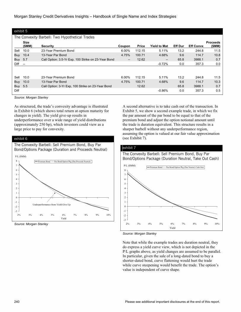
Morgan Stanley Credit Derivatives Insights – Handbook of Single Name and Index Strategies
240 Please see additional important disclosures at the end of this report.
exhibit 5
The Convexity Barbell: Two Hypothetical Trades Size($MM) Security Coupon Price Yield to Mat Eff Dur Eff Convx
Proceeds($MM)
Sell 10.0 23-Year Premium Bond 6.00% 112.15 5.11% 13.2 244.8 11.5Buy 10.4 13-Year Par Bond 4.75% 100.71 4.68% 9.6 114.7 10.8Buy 5.7 Call Option: 3.5-Yr Exp, 100 Strike on 23-Year Bond -- 12.62 -- 65.8 3988.1 0.7Diff -- -0.72% 0.0 357.3 0.0 Sell 10.0 23-Year Premium Bond 6.00% 112.15 5.11% 13.2 244.8 11.5Buy 10.0 13-Year Par Bond 4.75% 100.71 4.68% 9.6 114.7 10.3Buy 5.5 Call Option: 3-Yr Exp, 100 Strike on 23-Year Bond 12.62 65.8 3988.1 0.7Diff -0.86% 0.0 357.3 0.5
Source: Morgan Stanley
As structured, the trade’s convexity advantage is illustrated in Exhibit 6 (which shows total return at option maturity for changes in yield). The yield give-up results in underperformance over a wide range of yield distributions (approximately 250 bp), which investors could view as a large price to pay for convexity.
exhibit 6
The Convexity Barbell: Sell Premium Bond, Buy Par Bond/Options Package (Duration and Proceeds Neutral)
P/L ($MM)
-3
-2
-1
0
1
2
3
4
5
6
7
8
2% 3% 4% 5% 6% 7% 8% 9% 10%Yield
Premium Bond Par Bond/Option Pkg (Dur,Proceeds Neutral)
Underperformance from Yield Give Up
Source: Morgan Stanley
A second alternative is to take cash out of the transaction. In Exhibit 5, we show a second example trade, in which we fix the par amount of the par bond to be equal to that of the premium bond and adjust the option notional amount until the trade is duration equivalent. This structure results in a sharper barbell without any underperformance region, assuming the option is valued at our fair value approximation (see Exhibit 7).
exhibit 7
The Convexity Barbell: Sell Premium Bond, Buy Par Bond/Options Package (Duration Neutral, Take Out Cash)
P/L ($MM)
-3
-2
-1
0
1
2
3
4
5
6
7
8
2% 3% 4% 5% 6% 7% 8% 9% 10%
Yield
Premium Bond Par Bond/Option Pkg (Dur Neutral, Cash Out)
Source: Morgan Stanley
Note that while the example trades are duration neutral, they do express a yield curve view, which is not depicted in the P/L graphs above, as yield changes are assumed to be parallel. In particular, given the sale of a long-dated bond to buy a shorter-dated bond, curve flattening would hurt the trade while curve steepening would benefit the trade. The option’s value is independent of curve shape.
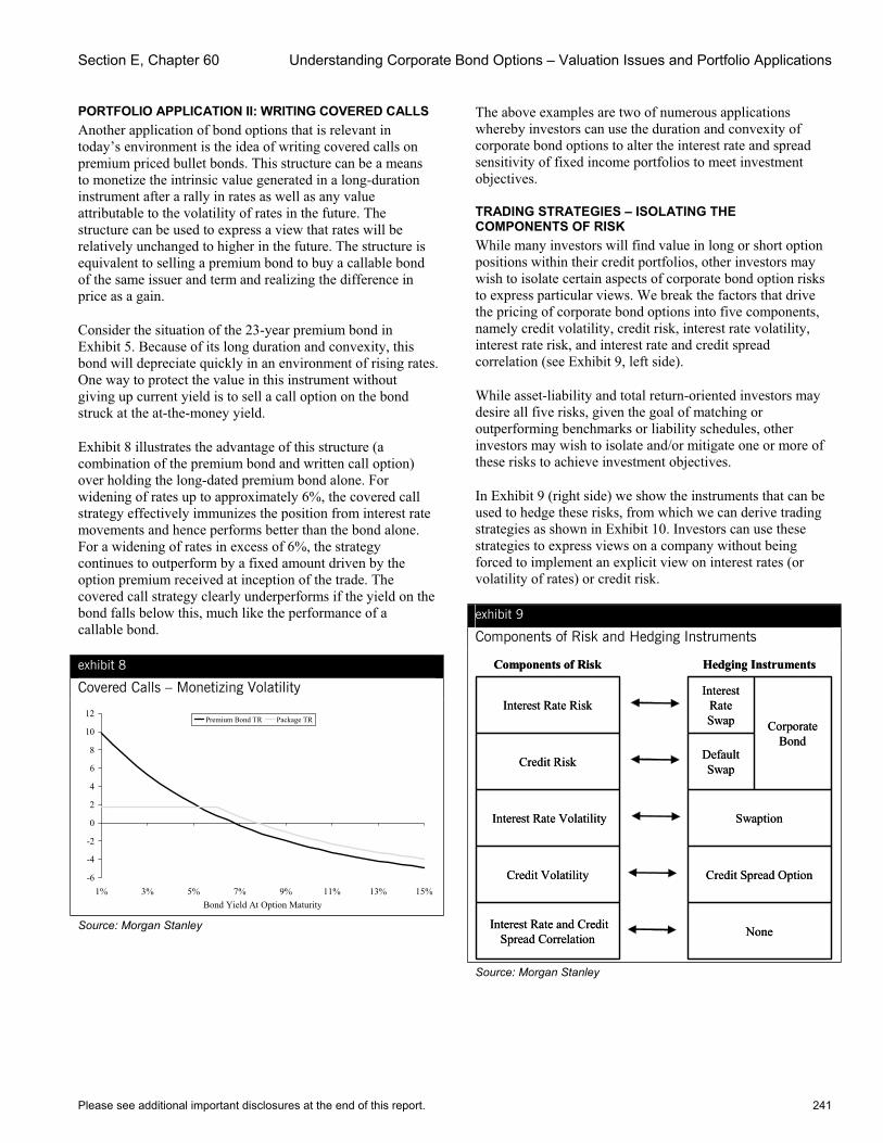
Section E, Chapter 60 Understanding Corporate Bond Options – Valuation Issues and Portfolio Applications
Please see additional important disclosures at the end of this report. 241
PORTFOLIO APPLICATION II: WRITING COVERED CALLS Another application of bond options that is relevant in today’s environment is the idea of writing covered calls on premium priced bullet bonds. This structure can be a means to monetize the intrinsic value generated in a long-duration instrument after a rally in rates as well as any value attributable to the volatility of rates in the future. The structure can be used to express a view that rates will be relatively unchanged to higher in the future. The structure is equivalent to selling a premium bond to buy a callable bond of the same issuer and term and realizing the difference in price as a gain.
Consider the situation of the 23-year premium bond in Exhibit 5. Because of its long duration and convexity, this bond will depreciate quickly in an environment of rising rates. One way to protect the value in this instrument without giving up current yield is to sell a call option on the bond struck at the at-the-money yield.
Exhibit 8 illustrates the advantage of this structure (a combination of the premium bond and written call option) over holding the long-dated premium bond alone. For widening of rates up to approximately 6%, the covered call strategy effectively immunizes the position from interest rate movements and hence performs better than the bond alone. For a widening of rates in excess of 6%, the strategy continues to outperform by a fixed amount driven by the option premium received at inception of the trade. The covered call strategy clearly underperforms if the yield on the bond falls below this, much like the performance of a callable bond.
exhibit 8
Covered Calls – Monetizing Volatility
-6
-4
-2
0
2
4
6
8
10
12
1% 3% 5% 7% 9% 11% 13% 15%Bond Yield At Option Maturity
Premium Bond TR Package TR
Source: Morgan Stanley
The above examples are two of numerous applications whereby investors can use the duration and convexity of corporate bond options to alter the interest rate and spread sensitivity of fixed income portfolios to meet investment objectives.
TRADING STRATEGIES – ISOLATING THE COMPONENTS OF RISK While many investors will find value in long or short option positions within their credit portfolios, other investors may wish to isolate certain aspects of corporate bond option risks to express particular views. We break the factors that drive the pricing of corporate bond options into five components, namely credit volatility, credit risk, interest rate volatility, interest rate risk, and interest rate and credit spread correlation (see Exhibit 9, left side).
While asset-liability and total return-oriented investors may desire all five risks, given the goal of matching or outperforming benchmarks or liability schedules, other investors may wish to isolate and/or mitigate one or more of these risks to achieve investment objectives.
In Exhibit 9 (right side) we show the instruments that can be used to hedge these risks, from which we can derive trading strategies as shown in Exhibit 10. Investors can use these strategies to express views on a company without being forced to implement an explicit view on interest rates (or volatility of rates) or credit risk.
exhibit 9
Components of Risk and Hedging Instruments
NoneInterest Rate and Credit Spread Correlation
Credit Spread OptionCredit Volatility
SwaptionInterest Rate Volatility
Default SwapCredit Risk
Corporate Bond
Interest Rate Swap
Interest Rate Risk
Hedging InstrumentsComponents of Risk
NoneInterest Rate and Credit Spread Correlation
Credit Spread OptionCredit Volatility
SwaptionInterest Rate Volatility
Default SwapCredit Risk
Corporate Bond
Interest Rate Swap
Interest Rate Risk
Hedging InstrumentsComponents of Risk
Source: Morgan Stanley

Morgan Stanley Credit Derivatives Insights – Handbook of Single Name and Index Strategies
242 Please see additional important disclosures at the end of this report.
exhibit 10
Corporate Bond Option Trading Strategies Trading Strategy Package Rationale Long credit volatility Long option, long credit protection, short
swaption, pay fixed in swap Pure long credit volatility play; expresses a view that
company’s valuation becomes markedly less certain
Long credit volatility and credit risk Long option, short swaption, pay fixed in swap
A levered long credit position; implements a view that company rallies strongly
Long credit and interest rate volatility, credit risk
Long option, pay fixed in swap Option position without interest rate risk; expresses view that company does well independent of economic cycle
Long credit and interest rate volatility Long option, long credit protection, pay fixed in swap
Pure long credit and interest rate volatility play; implements an “uncertain” economic view on a cyclical or interest rate sensitive company
Long credit and interest rate volatility, interest rate risk
Long option, long credit protection Option position without credit risk; expresses an increasingly uncertain credit view combined with a view on rates
Long credit volatility and interest rate risk Long option, long protection, short swaption Expresses a weak-economy view combined with increased credit uncertainty
Long credit and interest rate risk, credit and interest rate volatility
Long option Original option position with duration and convexity applications
Source: Morgan Stanley
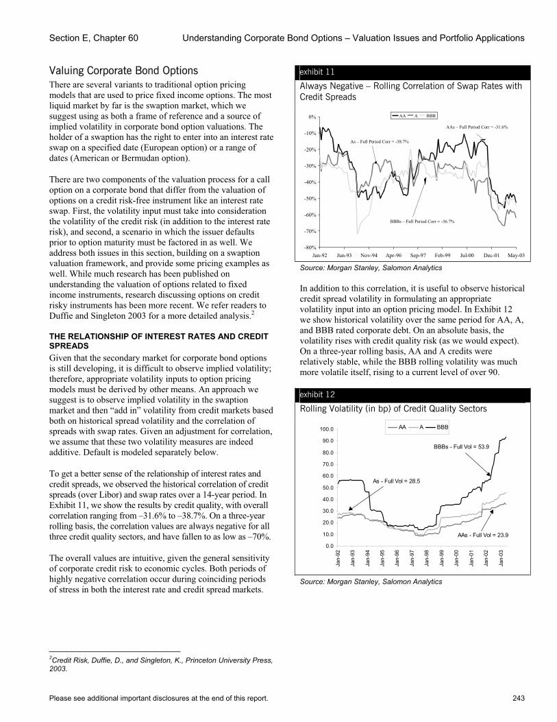
Section E, Chapter 60 Understanding Corporate Bond Options – Valuation Issues and Portfolio Applications
Please see additional important disclosures at the end of this report. 243
Valuing Corporate Bond Options There are several variants to traditional option pricing models that are used to price fixed income options. The most liquid market by far is the swaption market, which we suggest using as both a frame of reference and a source of implied volatility in corporate bond option valuations. The holder of a swaption has the right to enter into an interest rate swap on a specified date (European option) or a range of dates (American or Bermudan option).
There are two components of the valuation process for a call option on a corporate bond that differ from the valuation of options on a credit risk-free instrument like an interest rate swap. First, the volatility input must take into consideration the volatility of the credit risk (in addition to the interest rate risk), and second, a scenario in which the issuer defaults prior to option maturity must be factored in as well. We address both issues in this section, building on a swaption valuation framework, and provide some pricing examples as well. While much research has been published on understanding the valuation of options related to fixed income instruments, research discussing options on credit risky instruments has been more recent. We refer readers to Duffie and Singleton 2003 for a more detailed analysis.2
THE RELATIONSHIP OF INTEREST RATES AND CREDIT SPREADS Given that the secondary market for corporate bond options is still developing, it is difficult to observe implied volatility; therefore, appropriate volatility inputs to option pricing models must be derived by other means. An approach we suggest is to observe implied volatility in the swaption market and then “add in” volatility from credit markets based both on historical spread volatility and the correlation of spreads with swap rates. Given an adjustment for correlation, we assume that these two volatility measures are indeed additive. Default is modeled separately below.
To get a better sense of the relationship of interest rates and credit spreads, we observed the historical correlation of credit spreads (over Libor) and swap rates over a 14-year period. In Exhibit 11, we show the results by credit quality, with overall correlation ranging from –31.6% to –38.7%. On a three-year rolling basis, the correlation values are always negative for all three credit quality sectors, and have fallen to as low as –70%.
The overall values are intuitive, given the general sensitivity of corporate credit risk to economic cycles. Both periods of highly negative correlation occur during coinciding periods of stress in both the interest rate and credit spread markets.
2Credit Risk, Duffie, D., and Singleton, K., Princeton University Press, 2003.
exhibit 11
Always Negative – Rolling Correlation of Swap Rates with Credit Spreads
-80%
-70%
-60%
-50%
-40%
-30%
-20%
-10%
0%
Jan-92 Jun-93 Nov-94 Apr-96 Sep-97 Feb-99 Jul-00 Dec-01 May-03
AA A BBB
BBBs – Full Period Corr = -36.7%
As – Full Period Corr = -38.7%
AAs – Full Period Corr = -31.6%
Source: Morgan Stanley, Salomon Analytics
In addition to this correlation, it is useful to observe historical credit spread volatility in formulating an appropriate volatility input into an option pricing model. In Exhibit 12 we show historical volatility over the same period for AA, A, and BBB rated corporate debt. On an absolute basis, the volatility rises with credit quality risk (as we would expect). On a three-year rolling basis, AA and A credits were relatively stable, while the BBB rolling volatility was much more volatile itself, rising to a current level of over 90.
exhibit 12
Rolling Volatility (in bp) of Credit Quality Sectors
0.0
10.0
20.0
30.0
40.0
50.0
60.0
70.0
80.0
90.0
100.0
Jan-
92
Jan-
93
Jan-
94
Jan-
95
Jan-
96
Jan-
97
Jan-
98
Jan-
99
Jan-
00
Jan-
01
Jan-
02
Jan-
03
AA A BBB
BBBs - Full Vol = 53.9
AAs - Full Vol = 23.9
As - Full Vol = 28.5
Source: Morgan Stanley, Salomon Analytics

Morgan Stanley Credit Derivatives Insights – Handbook of Single Name and Index Strategies
244 Please see additional important disclosures at the end of this report.
VALUING THE OPTION With this background, we discuss below one method for valuing corporate bond options struck near par, based on the standard Black swaption framework. Given the inherent complexities in valuing American/Bermudan options on bonds, we have concentrated on the issues related to valuing European options here. This valuation could therefore be viewed as a floor on Bermudan or American options. In particular, we focus on three points:
• Determining an expected forward risky rate (or price) at option expiry
• Calculating an appropriate volatility given implied swaption volatility and assumptions for credit spread volatility and correlation
• Modeling the likelihood of default
EXPECTED FORWARD CREDIT RISKY RATE AT OPTION EXPIRATION The prevailing risky rate applicable to a corporate bond at the time of option expiration can be divided into the future prevailing swap rate and the Libor credit spread for the appropriate maturity.
The current forward swap rate can be observed directly from the prevailing swap curve today. We use this forward rate as an approximation of the expected future swap rate.
The expected future credit spread can potentially be derived in a manner similar to that of the swap rate if the credit has instruments with a variety of maturities. Alternatively, one can use current credit spreads to approximate the forward credit spread in a variety of ways. The methodology used and level of rigor with which the future credit spread is derived should weigh the absolute level of spreads and the impact on option valuation. Generally, the wider the credit spread, the greater the impact of the spread assumption on the option valuation.
The expected future credit risky rate can then be computed and utilized in the option valuation.
DETERMINING VOLATILITY Moving from volatility of swap rates to volatility of risky rates within the framework of the Black model is a challenge. In order to make use of the forward looking swap rate volatility data available from the swaption market, we rely on the assumption of lognormal swap rates. However, in order to use the Black framework to value the option on a default risky bond, we rely on the assumption that risky rates are also lognormal.
The method we employ allows us to approximate the expected value and variance of forward credit spreads and to calculate the expected value and volatility for the risky rate. We rely on the assumption that credit spreads are distributed in such a way that when added to a lognormal distribution, the result is once again lognormal.
The variance of the risky rate is derived using the following basic formulation:
adCreditSpreSwapadCreditSpreSwapRiskyRate VVVVV ρ2++=Where:
)1(22 −= SwapeFV SwapSwap
σ
Swapσ = swaption implied volatility (generally at the money; can be adjusted for skew)
ρ = correlation between the level of the swap rate and the level of credit spread
SwapF = Forward swap rate from option expiration through
bond maturity
Finally, the RiskyRateσ parameter is calculated based on inverting the formula above:
+= 12RiskyRate
RiskyRateRiskyRate F
VLnσ
Exhibit 13 illustrates the sensitivity of the risky rate volatility (the RiskyRateσ parameter) for various credit spread and credit spread volatility assumptions for a given swap rate, swap volatility and correlation. We find that for reasonable combinations of credit spread and credit spread volatility, the impact of varying correlation within the range from –10% to –40% results in relatively small changes in volatility for typical investment grade spread levels. Exhibit 14 illustrates the sensitivity of the risky rate volatility across a broad range of correlation for a credit with a spread of 100 bp.
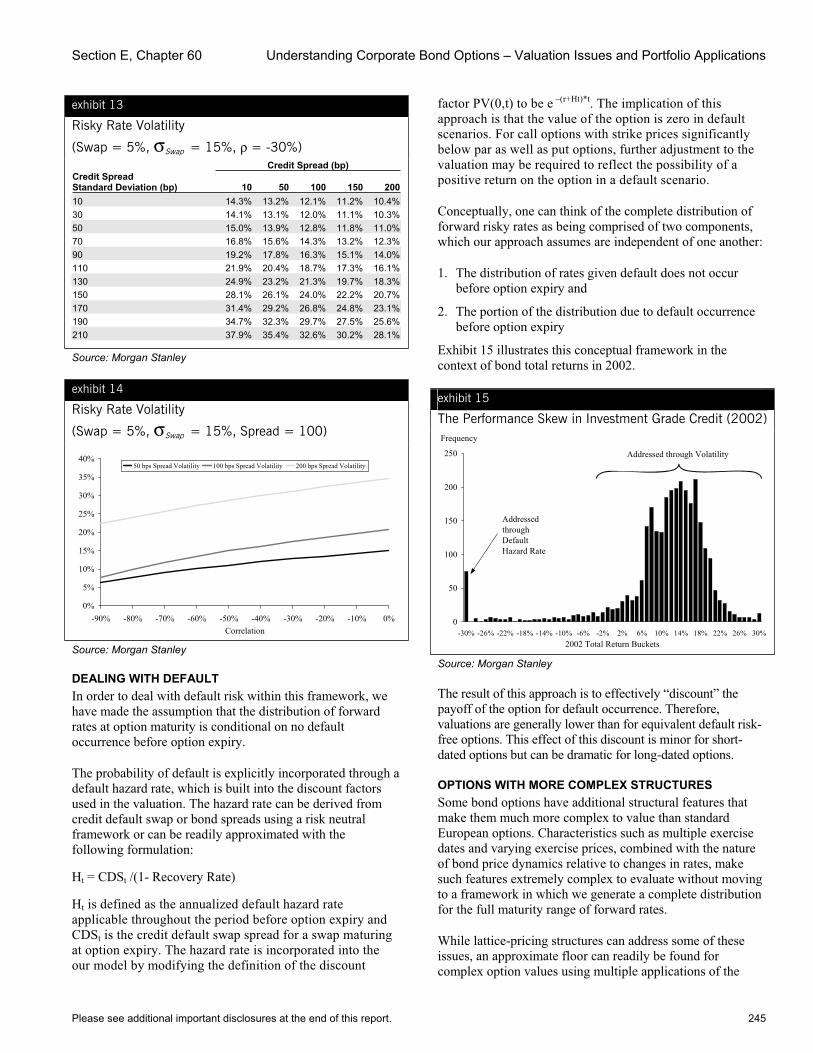
Section E, Chapter 60 Understanding Corporate Bond Options – Valuation Issues and Portfolio Applications
Please see additional important disclosures at the end of this report. 245
exhibit 13
Risky Rate Volatility
(Swap = 5%, σSwap = 15%, ρ = -30%) Credit Spread (bp) Credit Spread Standard Deviation (bp) 10 50 100 150 20010 14.3% 13.2% 12.1% 11.2% 10.4%30 14.1% 13.1% 12.0% 11.1% 10.3%50 15.0% 13.9% 12.8% 11.8% 11.0%70 16.8% 15.6% 14.3% 13.2% 12.3%90 19.2% 17.8% 16.3% 15.1% 14.0%110 21.9% 20.4% 18.7% 17.3% 16.1%130 24.9% 23.2% 21.3% 19.7% 18.3%150 28.1% 26.1% 24.0% 22.2% 20.7%170 31.4% 29.2% 26.8% 24.8% 23.1%190 34.7% 32.3% 29.7% 27.5% 25.6%210 37.9% 35.4% 32.6% 30.2% 28.1%
Source: Morgan Stanley
exhibit 14
Risky Rate Volatility
(Swap = 5%, σSwap = 15%, Spread = 100)
0%
5%
10%
15%
20%
25%
30%
35%
40%
-90% -80% -70% -60% -50% -40% -30% -20% -10% 0%Correlation
50 bps Spread Volatility 100 bps Spread Volatility 200 bps Spread Volatility
Source: Morgan Stanley
DEALING WITH DEFAULT In order to deal with default risk within this framework, we have made the assumption that the distribution of forward rates at option maturity is conditional on no default occurrence before option expiry.
The probability of default is explicitly incorporated through a default hazard rate, which is built into the discount factors used in the valuation. The hazard rate can be derived from credit default swap or bond spreads using a risk neutral framework or can be readily approximated with the following formulation:
Ht = CDSt /(1- Recovery Rate)
Ht is defined as the annualized default hazard rate applicable throughout the period before option expiry and CDSt is the credit default swap spread for a swap maturing at option expiry. The hazard rate is incorporated into the our model by modifying the definition of the discount
factor PV(0,t) to be e –(r+Ht)*t. The implication of this approach is that the value of the option is zero in default scenarios. For call options with strike prices significantly below par as well as put options, further adjustment to the valuation may be required to reflect the possibility of a positive return on the option in a default scenario.
Conceptually, one can think of the complete distribution of forward risky rates as being comprised of two components, which our approach assumes are independent of one another:
1. The distribution of rates given default does not occur before option expiry and
2. The portion of the distribution due to default occurrence before option expiry
Exhibit 15 illustrates this conceptual framework in the context of bond total returns in 2002.
exhibit 15
The Performance Skew in Investment Grade Credit (2002)Frequency
0
50
100
150
200
250
-30% -26% -22% -18% -14% -10% -6% -2% 2% 6% 10% 14% 18% 22% 26% 30%2002 Total Return Buckets
AddressedthroughDefaultHazard Rate
Addressed through Volatility
Source: Morgan Stanley
The result of this approach is to effectively “discount” the payoff of the option for default occurrence. Therefore, valuations are generally lower than for equivalent default risk-free options. This effect of this discount is minor for short-dated options but can be dramatic for long-dated options.
OPTIONS WITH MORE COMPLEX STRUCTURES Some bond options have additional structural features that make them much more complex to value than standard European options. Characteristics such as multiple exercise dates and varying exercise prices, combined with the nature of bond price dynamics relative to changes in rates, make such features extremely complex to evaluate without moving to a framework in which we generate a complete distribution for the full maturity range of forward rates.
While lattice-pricing structures can address some of these issues, an approximate floor can readily be found for complex option values using multiple applications of the
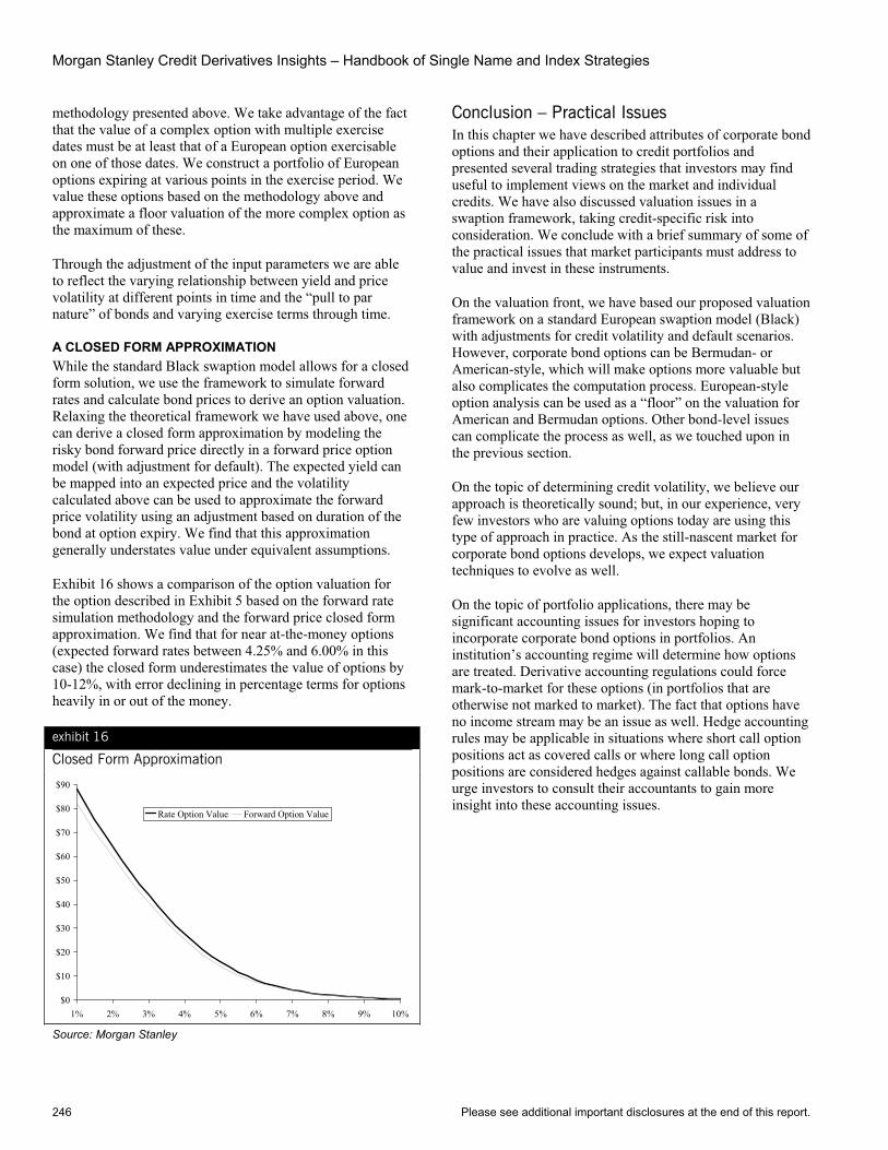
Morgan Stanley Credit Derivatives Insights – Handbook of Single Name and Index Strategies
246 Please see additional important disclosures at the end of this report.
methodology presented above. We take advantage of the fact that the value of a complex option with multiple exercise dates must be at least that of a European option exercisable on one of those dates. We construct a portfolio of European options expiring at various points in the exercise period. We value these options based on the methodology above and approximate a floor valuation of the more complex option as the maximum of these.
Through the adjustment of the input parameters we are able to reflect the varying relationship between yield and price volatility at different points in time and the “pull to par nature” of bonds and varying exercise terms through time.
A CLOSED FORM APPROXIMATION While the standard Black swaption model allows for a closed form solution, we use the framework to simulate forward rates and calculate bond prices to derive an option valuation. Relaxing the theoretical framework we have used above, one can derive a closed form approximation by modeling the risky bond forward price directly in a forward price option model (with adjustment for default). The expected yield can be mapped into an expected price and the volatility calculated above can be used to approximate the forward price volatility using an adjustment based on duration of the bond at option expiry. We find that this approximation generally understates value under equivalent assumptions.
Exhibit 16 shows a comparison of the option valuation for the option described in Exhibit 5 based on the forward rate simulation methodology and the forward price closed form approximation. We find that for near at-the-money options (expected forward rates between 4.25% and 6.00% in this case) the closed form underestimates the value of options by 10-12%, with error declining in percentage terms for options heavily in or out of the money.
exhibit 16
Closed Form Approximation
$0
$10
$20
$30
$40
$50
$60
$70
$80
$90
1% 2% 3% 4% 5% 6% 7% 8% 9% 10%
Rate Option Value Forward Option Value
Source: Morgan Stanley
Conclusion – Practical Issues In this chapter we have described attributes of corporate bond options and their application to credit portfolios and presented several trading strategies that investors may find useful to implement views on the market and individual credits. We have also discussed valuation issues in a swaption framework, taking credit-specific risk into consideration. We conclude with a brief summary of some of the practical issues that market participants must address to value and invest in these instruments.
On the valuation front, we have based our proposed valuation framework on a standard European swaption model (Black) with adjustments for credit volatility and default scenarios. However, corporate bond options can be Bermudan- or American-style, which will make options more valuable but also complicates the computation process. European-style option analysis can be used as a “floor” on the valuation for American and Bermudan options. Other bond-level issues can complicate the process as well, as we touched upon in the previous section.
On the topic of determining credit volatility, we believe our approach is theoretically sound; but, in our experience, very few investors who are valuing options today are using this type of approach in practice. As the still-nascent market for corporate bond options develops, we expect valuation techniques to evolve as well.
On the topic of portfolio applications, there may be significant accounting issues for investors hoping to incorporate corporate bond options in portfolios. An institution’s accounting regime will determine how options are treated. Derivative accounting regulations could force mark-to-market for these options (in portfolios that are otherwise not marked to market). The fact that options have no income stream may be an issue as well. Hedge accounting rules may be applicable in situations where short call option positions act as covered calls or where long call option positions are considered hedges against callable bonds. We urge investors to consult their accountants to gain more insight into these accounting issues.
Please see additional important disclosures at the end of this report. 247
Chapter 61
Options for Nothing, Interest Rate Risk for Free March 26, 2004
Primary Analyst: Sivan Mahadevan Primary Analyst: Brian Arsenault Primary Analyst: Peter Polanskyj Anisha Ambardar
One of the complications in making relative value decisions between bonds and default swaps is dealing with the differences embedded in the various instruments. Default swaps generally have restructuring risk and overwhelmingly trade as bullet instruments (the cancelable CDS market is just beginning). Corporate bonds can have variable coupons (i.e., step-ups) and can be callable as well. In a world of relatively tight spreads, these structural differences become an important factor in determining relative value. One of the most important differences, in our view, is the call risk (or alternatively, the extension risk) in corporate bonds, particularly in high yield, where over 60% of the market is callable.
In Chapter 40, we introduced our high yield basis (between CDS and cash) and discussed the idea that the basis for callable bonds can be very volatile, depending on how much the call option is “in the money.” For investors deciding between selling bullet protection or buying callable bonds, the market does not provide much help.
However, the relationship between callable bonds and CDS provides us with a framework to imply a value for the options callable bond investors are writing. As such, we find the comparison to be a useful relative value exercise when deciding between callable bonds and default swaps (or bullet bonds). High yield market convention is to quote callable bonds on a “to-worst” basis, partly because it is difficult to make good volatility assumptions for option-adjusted calculations.
Using our simple framework, there are numerous examples of callable bonds where investors are not being adequately compensated for the call risk, in our view. As such, we question whether the high yield basis is really negative for many issuers, when considering a “fairer value” for the optionality of callable bonds.
THE BASIC METHODOLOGY – OAS MAKES A COMEBACK The approach we use to determine relative value between bullet default swaps and callable bonds is fairly straightforward, and is based on the notion of option-adjusted spread (for those who are new to the credit markets, this is a 1980s concept that does not get a lot of attention today). The end game is to value the call option that the callable bond investor is writing, based on where the bullet protection trades. For example, if the resulting implied volatility/option price seems low, then the bond holder is writing the option too cheaply, which tells us that selling protection is better value.
Implementing what we just described above is fairly simple, requiring one Bloomberg screen (OAS1) to compute the implied volatility given a bond’s dollar price and the assumed credit spread curve (which is used to shift the swap curve to reflect the default risk inherent in all the cash flows). Forming an opinion on this implied volatility requires a bit more intuition, as there is both an interest rate and credit component to it. We go through some historical examples in the next section.
This approach may seem like it brings too much quantitative analysis to a market that really trades on credit fundamentals, but we find many situations where the relative value information is strikingly clear and very intuitive. Furthermore, the extension risk in many callable high yield bonds can really be driven by interest rate movements at today’s spread levels, not credit fundamentals, which is a risk that does not appear to be adequately priced into the high yield market.
VOLATILITY AND INTEREST RATE RISK – IMPLICATIONS FOR CALLABLE HIGH YIELD BONDS Going down the path we propose above has the risk of introducing a lot of volatility confusion, as one thinks about various measures. To keep things simple, we highlight a few points with respect to volatility that are important to understand in this context.
• The volatility that a callable bond investor is exposed to is related to price movements for the bond. This volatility, therefore, has both an interest rate component and a credit spread component.
• Combining both interest rate and credit spread volatility requires making assumptions about how they are related. In general, we have found they are negatively correlated, but corporate bonds are still more volatile on an absolute basis, particularly for wider trading credits.1
• We find that average high yield realized volatility (for a selected universe of 16 bullet instruments) has been greater than the realized volatility in the swap market in recent history. Today, these two markets appear to be near parity in terms of volatility (see Exhibit 1).
• Callable high yield bonds today can have significant extension risk related to interest rate movements, given the absolute level of spreads, high dollar prices, and the idea that an inflection point in interest rates may not be that far away. This risk is not captured by measures like spread-to-worst.
1Please refer to Chapter 60.

Morgan Stanley Credit Derivatives Insights – Handbook of Single Name and Index Strategies
248 Please see additional important disclosures at the end of this report.
exhibit 1
High Yield Volatility Approaches Swap Volatility Levels
Vol
0%
10%
20%
30%
40%
50%
60%
Dec-01 Jun-02 Nov-02 Apr-03 Oct-03 Mar-04
Average 7Y Swap
Source: Morgan Stanley, Bloomberg, Salomon Analytics
UNCOVERING THE RELATIVE VALUE We apply our simple relative value approach to a dozen callable high yield bonds to see how the market is pricing in the call risk (see Exhibit 2). We find that callable issues for DirectTV, Echostar and Williams Companies have implied
volatilities and option pricing that seem reasonable to us, given the risks. DirectTV’s callable 2013 bond, for example, trades 153 bp wider than CDS on a Z-spread-to-worst basis (mid-market), but this spread cushion results in an option value of 8.72 points, which appears relatively fair compared to a 30% volatility assumption.
For several other credits, we find pricing on callable bonds that ascribes very little or even negative value to the option the bond holder is writing. For example, Host Marriot’s 2013 callable bonds trade 32 bp tighter than CDS (on a mid-market Libor basis), implying a negative option value (i.e., the bond investor is paying to be short the option). Therefore, an investor can pick up spread and eliminate the short option position by swapping from the callable bonds into CDS.
While it is hard to calculate what the real volatility for a callable high yield bond ought to be, we take comfort in using swaption levels as a conservative measure for two reasons. First, credit-related issues, positive or negative, can have at least as large an impact on a bond’s price as sharp interest rate moves. Second, the options investors are writing on high yield bonds are American in nature (with multiple dates) and are difficult to accurately model, but are more expensive intuitively.
exhibit 2
Valuing the Call Option – Comparing Callable Bonds to Bullet Instruments
Ticker Coupon Maturity Recent
Price Z Spread Bullet Z Spread
CDSMid
Implied Vol (%)
Implied Option Price
Option Price at 30% Vol Comments
WMB 8.625 6/1/2010 110.250 356 255 29% 3.53 3.65 Reasonable Valuation AW 7.875 4/15/2013 109.000 353 272 290 N/A Less than zero 4.70 Callable Too Rich NXTL 6.875 10/31/2013 106.625 258 175 14% 1.53 4.40 DISH 9.125 1/15/2009 113.375 212 180 20% 5.21 6.06 Reasonable Valuation LYO 9.5 12/15/2008 99.500 574 675 N/A Less than zero 1.60 Callable Too Rich HMT 7.125 11/1/2013 103.500 293 269 325 N/A Less than zero 3.54 Callable Too Rich XRX 7.625 6/15/2013 106.500 296 254 255 12% 1.20 4.51 EQCHEM 10.625 5/1/2011 105.500 628 556 17% 2.11 4.22 AMT 7.25 12/1/2011 102.000 365 425 N/A Less than zero 2.00 Callable Too Rich AMKR 7.75 5/15/2013 101.500 399 353 8% 0.23 3.62 Callable Too Rich DTV 8.375 3/15/2013 113.125 296 143 35% 8.72 7.75 Reasonable Valuation
Source: Morgan Stanley, Bloomberg
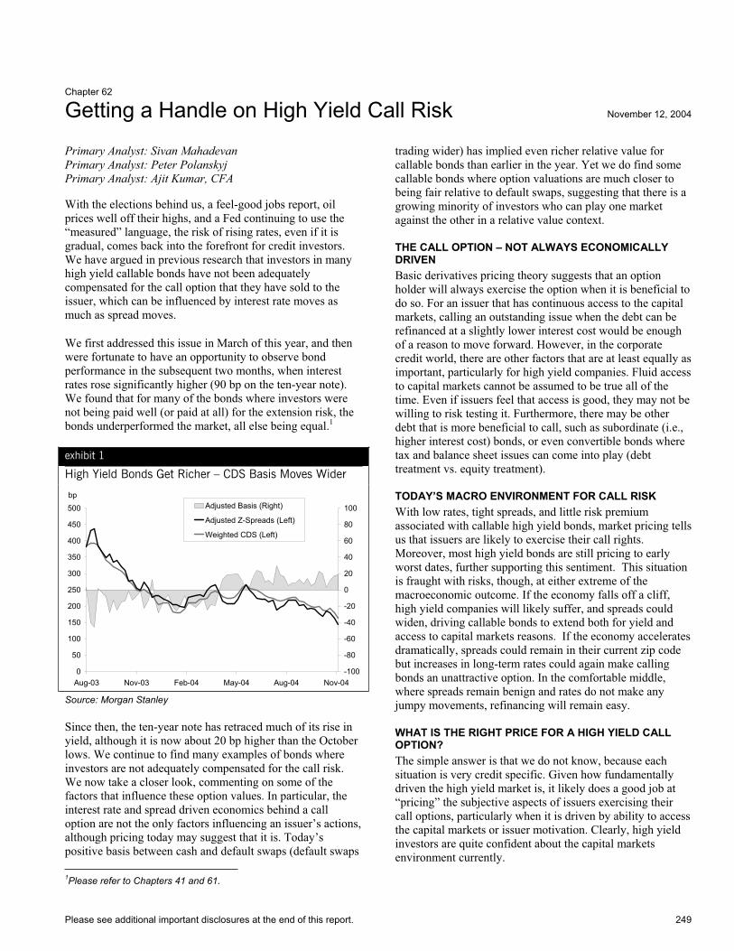
Please see additional important disclosures at the end of this report. 249
Chapter 62
Getting a Handle on High Yield Call Risk November 12, 2004
Primary Analyst: Sivan Mahadevan Primary Analyst: Peter Polanskyj Primary Analyst: Ajit Kumar, CFA
With the elections behind us, a feel-good jobs report, oil prices well off their highs, and a Fed continuing to use the “measured” language, the risk of rising rates, even if it is gradual, comes back into the forefront for credit investors. We have argued in previous research that investors in many high yield callable bonds have not been adequately compensated for the call option that they have sold to the issuer, which can be influenced by interest rate moves as much as spread moves.
We first addressed this issue in March of this year, and then were fortunate to have an opportunity to observe bond performance in the subsequent two months, when interest rates rose significantly higher (90 bp on the ten-year note). We found that for many of the bonds where investors were not being paid well (or paid at all) for the extension risk, the bonds underperformed the market, all else being equal.1
exhibit 1
High Yield Bonds Get Richer – CDS Basis Moves Wider
bp
0
50
100
150
200
250
300
350
400
450
500
Aug-03 Nov-03 Feb-04 May-04 Aug-04 Nov-04-100
-80
-60
-40
-20
0
20
40
60
80
100Adjusted Basis (Right)
Adjusted Z-Spreads (Left)
Weighted CDS (Left)
Source: Morgan Stanley
Since then, the ten-year note has retraced much of its rise in yield, although it is now about 20 bp higher than the October lows. We continue to find many examples of bonds where investors are not adequately compensated for the call risk. We now take a closer look, commenting on some of the factors that influence these option values. In particular, the interest rate and spread driven economics behind a call option are not the only factors influencing an issuer’s actions, although pricing today may suggest that it is. Today’s positive basis between cash and default swaps (default swaps 1Please refer to Chapters 41 and 61.
trading wider) has implied even richer relative value for callable bonds than earlier in the year. Yet we do find some callable bonds where option valuations are much closer to being fair relative to default swaps, suggesting that there is a growing minority of investors who can play one market against the other in a relative value context.
THE CALL OPTION – NOT ALWAYS ECONOMICALLY DRIVENBasic derivatives pricing theory suggests that an option holder will always exercise the option when it is beneficial to do so. For an issuer that has continuous access to the capital markets, calling an outstanding issue when the debt can be refinanced at a slightly lower interest cost would be enough of a reason to move forward. However, in the corporate credit world, there are other factors that are at least equally as important, particularly for high yield companies. Fluid access to capital markets cannot be assumed to be true all of the time. Even if issuers feel that access is good, they may not be willing to risk testing it. Furthermore, there may be other debt that is more beneficial to call, such as subordinate (i.e., higher interest cost) bonds, or even convertible bonds where tax and balance sheet issues can come into play (debt treatment vs. equity treatment).
TODAY’S MACRO ENVIRONMENT FOR CALL RISK With low rates, tight spreads, and little risk premium associated with callable high yield bonds, market pricing tells us that issuers are likely to exercise their call rights. Moreover, most high yield bonds are still pricing to early worst dates, further supporting this sentiment. This situation is fraught with risks, though, at either extreme of the macroeconomic outcome. If the economy falls off a cliff, high yield companies will likely suffer, and spreads could widen, driving callable bonds to extend both for yield and access to capital markets reasons. If the economy accelerates dramatically, spreads could remain in their current zip code but increases in long-term rates could again make calling bonds an unattractive option. In the comfortable middle, where spreads remain benign and rates do not make any jumpy movements, refinancing will remain easy.
WHAT IS THE RIGHT PRICE FOR A HIGH YIELD CALL OPTION?The simple answer is that we do not know, because each situation is very credit specific. Given how fundamentally driven the high yield market is, it likely does a good job at “pricing” the subjective aspects of issuers exercising their call options, particularly when it is driven by ability to access the capital markets or issuer motivation. Clearly, high yield investors are quite confident about the capital markets environment currently.
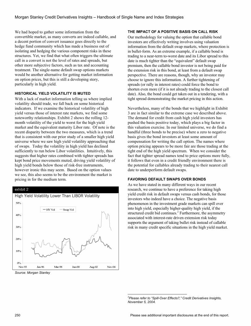
Morgan Stanley Credit Derivatives Insights – Handbook of Single Name and Index Strategies
250 Please see additional important disclosures at the end of this report.
We had hoped to gather some information from the convertible market, as many converts are indeed callable, and a decent portion of convert issuance goes directly to the hedge fund community which has made a business out of isolating and hedging the various component risks in these structures. Yet, we find that what often triggers the ultimate call in a convert is not the level of rates and spreads, but other more subjective factors, such as tax and accounting treatment. The single-name default swap options markets would be another alternative for getting market information on option prices, but this is still a developing story, particularly in high yield.
HISTORICAL YIELD VOLATILITY IS MUTED With a lack of market information telling us where implied volatility should trade, we fall back on some historical indicators. If we examine the historical volatility of high yield versus those of interest rate markets, we find some noteworthy relationships. Exhibit 2 shows the rolling 12-month volatility of the yield to worst for the high yield market and the equivalent maturity Libor rate. Of note is the recent disparity between the two measures, which is a trend that is consistent with our prior study of a smaller high yield universe where we saw high yield volatility approaching that of swaps. Today the volatility in high yield has declined sufficiently to run below Libor volatilities. Intuitively, this suggests that higher rates combined with tighter spreads has kept bond price movements muted, driving yield volatility of high yield bonds below those of risk-free instruments, however ironic this may seem. Based on the option values we see, this also seems to be the environment the market is pricing in for the medium term.
exhibit 2
High Yield Volatility Lower Than LIBOR Volatility
0%
10%
20%
30%
40%
50%
Nov-93 Jan-96 Mar-98 Jun-00 Aug-02 Nov-04
HY Vol Swap Vol
Source: Morgan Stanley
THE IMPACT OF A POSITIVE BASIS ON CALL RISK Our methodology for valuing the option that callable bond investors are effectively writing involves using valuation information from the default swap markets, where protection is in bullet-form. As an extreme example, if a callable bond is trading to a near-term to-worst date and its Libor spread to this date is much tighter than the “equivalent” default swap premium, then the callable bond investor is not being paid for the extension risk in this bond, at least from a default swap perspective. There are reasons, though, why an investor may choose to ignore this information. A further tightening of spreads (or rally in interest rates) could force the bond to shorten even more (if it is not already trading to the closest call date). Also, the bond could get taken out in a tendering, with a tight spread demonstrating the market pricing in this action.
Nevertheless, many of the bonds that we highlight in Exhibit 3 are in fact similar to the extreme case we described above. The demand for credit from cash high yield investors has pushed the basis positive today, which plays a big factor in this valuation exercise. In our limited universe, we do find a handful (three bonds to be precise) where a zero to negative basis gives the bond investors at least some amount of compensation for writing the call option. The names where option pricing appears to be more fair are those trading at the tight end of the high yield spectrum. When we consider the fact that tighter spread names tend to price options more fully, it follows that even in a credit friendly environment there is the potential for callables already trading to their nearest call date to underperform default swaps.
FAVORING DEFAULT SWAPS OVER BONDS As we have stated in many different ways in our recent research, we continue to have a preference for taking high yield credit risk in default swaps versus cash bonds, for those investors who indeed have a choice. The negative basis phenomenon in the investment grade markets can spill over into high yield, especially higher-quality high yield, if the structured credit bid continues.2 Furthermore, the asymmetry associated with interest-rate driven extension risk today supports the argument of taking bullet risk instead of callable risk in many credit specific situations in the high yield market.
2Please refer to “Spill-Over Effects?,” Credit Derivatives Insights, November 5, 2004.
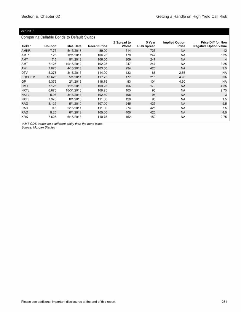
Section E, Chapter 62 Getting a Handle on High Yield Call Risk
Please see additional important disclosures at the end of this report. 251
exhibit 3
Comparing Callable Bonds to Default Swaps
Ticker Coupon Mat. Date Recent PriceZ Spread to
Worst5 Year
CDS SpreadImplied Option
PricePrice Diff for Non
Negative Option ValueAMKR 7.75 5/15/2013 89.00 514 725 NA 12AMT* 7.25 12/1/2011 106.25 179 247 NA 5.25AMT 7.5 5/1/2012 106.00 209 247 NA 4AMT 7.125 10/15/2012 102.25 247 247 NA 3.25AW 7.875 4/15/2013 103.50 294 420 NA 9.5DTV 8.375 3/15/2013 114.00 133 85 2.56 NAEQCHEM 10.625 5/1/2011 117.25 177 215 4.95 NAGP 9.375 2/1/2013 118.75 83 104 4.60 NAHMT 7.125 11/1/2013 109.25 156 170 NA 4.25NXTL 6.875 10/31/2013 109.25 105 95 NA 2.75NXTL 5.95 3/15/2014 102.50 108 95 NA 3NXTL 7.375 8/1/2015 111.00 129 95 NA 1.5RAD 8.125 5/1/2010 107.00 245 425 NA 9.5RAD 9.5 2/15/2011 111.00 274 425 NA 7.5RAD 9.25 6/1/2013 105.00 400 425 NA 4.5XRX 7.625 6/15/2013 110.75 162 150 NA 2.75
*AMT CDS trades on a different entity than the bond issue. Source: Morgan Stanley

Morgan Stanley Credit Derivatives Insights – Handbook of Single Name and Index Strategies
252 Please see additional important disclosures at the end of this report.
Chapter 63
Covered Calls Aren’t Crowded Trades June 24, 2005
Primary Analyst: Sivan Mahadevan Primary Analyst: Peter Polanskyj Primary Analyst: Ajit Kumar, CFA
As we approach the mid-point of a year that has been characterized by contrarian events, some fundamentally sound investment strategies have quickly morphed into crowded trades. From shorting the US dollar to shorting interest rates and mezzanine tranches, technicals have dominated fundamentals, and market movements have been surprising.
Long-term Treasury yield movements have perhaps been the most puzzling, as the sell-off that short-sellers welcomed in the first quarter was more than offset by a huge rally in the second quarter. While interest rates have all kinds of implications on credit spreads and bond pricing, one that clearly receives significantly less focus is the pricing of corporate bond options, including bonds with embedded options. The steady and sizable flattening of the Treasury curve and the inherent characteristics of corporate bond options can make them a strategically appealing way to implement credit and interest rate views.
CORPORATE BOND OPTION STRATEGIES When we first discussed corporate bond options in 2003, the environment appeared ripe for strategies like selling covered calls or swapping premium bonds for par instruments paired with the purchase of call options; 10-year Treasury rates were around 3.5%, and the then on-the-run DJ TRAC-XSM
Index traded at 50 bp.1 Jumping ahead two years, we see a market for corporate bond options that has continued to develop, albeit without the benefit of the hyper-liquidity created by the index and tranched index markets.
The goal of any option-based strategy is to change the carry, duration and convexity profile of a given instrument. As we look beyond the world of structured credit into the broader macro environment, we again see an environment where corporate bond option strategies look attractive to us. Corporate bonds, being hybrid instruments, are affected both by changes in the rate environment and changes in credit spread markets. We examine the importance and impact of the two markets on corporate bond options below.
1Please refer to Chapter 60.
REDEFINING AT-THE-MONEY In Exhibit 1, we show the 2’s-10’s curve steepness in both interest rate swap and Treasury markets over the last four years. While we have not reached the flat/inverted curve shape of 2000, the curve has flattened dramatically over the last year, bringing us to territory we have not seen since early 2001. One key implication of a flattening Treasury curve is the level of rates implied for future periods. While in 2002-4, markets implied markedly higher rates (and lower bond prices) several years forward, today’s relatively flat curve environment implies rates close to today’s levels (and bond prices near today’s levels, as well). While this effect will be somewhat offset by the increased steepness of credit curves today, the order of magnitude of interest rate impact is greater than the offsetting spread impact for a typical investment grade credit.
exhibit 1
Flattening Interest Rate Curves
-100
-50
0
50
100
150
200
250
300
350
Jan-00 Nov-00 Oct-01 Sep-02 Aug-03 Jul-04 Jun-05
2's10's Swaps
2's10's Treasuries
bp
-100
-50
0
50
100
150
200
250
300
350
Jan-00 Nov-00 Oct-01 Sep-02 Aug-03 Jul-04 Jun-05
2's10's Swaps
2's10's Treasuries
bp
Source: Morgan Stanley
In terms of corporate bond option markets, the effect of a flatter interest rate curve is to change our expectations of the future price of bonds and, by implication, the level at which an option with a given strike is in- or out-of-the-money. While a corporate bond call option struck marginally out-of-the-money in 2004 (compared to the spot price) may have appeared significantly out-of-the-money three years forward, the same option would appear to be much closer to at-the-money (three years forward) today, based solely on the relatively flat forward rates implied by today’s yield curve. This has significant valuation implications for the options, which we discuss below.
VOLATILITY – FRIEND OR FOE? Given all the market chatter about the low levels of volatility across asset classes, the idea of selling optionality may not be

Section E, Chapter 63 Covered Calls Aren’t Crowded Trades
Please see additional important disclosures at the end of this report. 253
attractive to some investors. In Exhibit 2, we compare the VIX to ATM implied volatility for 3- into 7-year swaptions and realized spread volatility, as measured by the DJ TRAC-X and CDX family of indices. While the implied volatility has declined in both equity and interest rate markets, these trends could continue, given the changes in realized volatility in these markets. Reflecting this, our interest rate strategy team has been constructive on opportunities to sell short-dated volatility (see The Interest Rate Strategist, June 16, 2005).
exhibit 2
Interest Rate and Equity Implied Volatility
10
20
30
40
50
60
Jan-00 Nov-00 Oct-01 Sep-02 Aug-03 Jul-04 Jun-05
VIXATM 3Y into 7Y VolCDX Realized
Source: Morgan Stanley
While spread levels and spread volatility are a driver of valuation in bond options, at today’s spread levels they may be less likely to be the key driver, given the asymmetry of credit risk and the absolute level of spreads relative to rate levels. At least in terms of volatility, corporate bond option prices on typical investment grade credits should be driven more by interest rate volatility than by spread volatility. To demonstrate this, we show the sensitivity of the implied credit risky rate volatility for a 10-year instrument using the CDX 10-year spread and the current 10-year swap rate (see Exhibit 3). The change in the risky rate volatility for a 1% change in the rate volatility has roughly five times the impact of a 1% change in the spread volatility.
exhibit 3
Relative Impact of Spread & Rate Volatility on Bond Option Volatility Correlation (Rates & Spreads) -50% -30.0% -10.0%1% Change in Rate Vol 0.5% 0.5% 0.6%1% Change in Spread Vol 0.1% 0.1% 0.1%Rate Vol Impact /Spread Vol Impact 5.6x 4.8x 4.4x
Source: Morgan Stanley
VALUATION IMPLICATIONS To measure the impact of the vastly different rate environment on the pricing of corporate bond options, we
examine the pricing for a hypothetical bond option in two different rate environments (based on the framework in Chapter 60). We analyze pricing in today’s prevailing environment, as well as in a hypothetical environment in which the underlying bond would have the same price but the interest rate curves would have the shape we experienced two years ago in June 2003, when we first published our thoughts on this topic.
We have summarized the results in Exhibit 4, for a 10-year bond trading at 81 bp above 10-year Libor. (The spread matches the current 10-year CDX level.) The premium for a call option, with the same strike and maturity, is about 60% higher today than in an environment similar to 2003, due largely to the significantly flatter curve, as the 2’s and 10’s curve has flattened more than 80% from June 2003 levels.
As we mentioned earlier, a steep yield curve (incorporating both interest rate levels and credit curve) for an issuer results in higher implied forward yields and lower implied forward prices, resulting in lower absolute option premiums for call options on bonds. The opposite is true for a relatively flat yield curve and explains the steep increase in the call premium (Exhibit 4).
exhibit 4
The Curve Environment: Implications for Bond Option Prices
(bp)
240
139157
43
105
248
0
50
100
150
200
250
300
Libor Curve Steepness(2's-10's)
Investment GradeCorporate Spread
Call Premium
Jun-03Jun-05
Source: Morgan Stanley, The YieldBook
MOVING THE BREAKEVENS In Exhibit 5, we show the payoff of a covered call strategy at the maturity of the call option. The option has a 3-year maturity and the underlying bond is a 10-year bond with coupon, spread and dollar price roughly matching that of the typical investment grade credit.
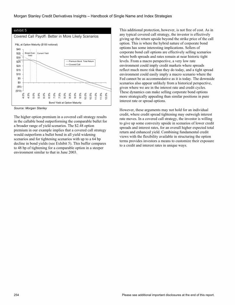
Morgan Stanley Credit Derivatives Insights – Handbook of Single Name and Index Strategies
254 Please see additional important disclosures at the end of this report.
exhibit 5
Covered Call Payoff: Better in More Likely Scenarios
P&L at Option Maturity ($100 notional)
($10)($5)$0$5
$10$15$20$25$30$35$40
4.0%
4.5%
5.0%
5.5%
6.0%
6.5%
7.0%
7.5%
8.0%
8.5%
9.0%
9.5%
10.0
%
10.5
%
11.0
%
11.5
%
12.0
%Bond Yield at Option Maturity
Premium Bond Total ReturnCovered Call
Current YieldBreak Even Yield
Source: Morgan Stanley
The higher option premium in a covered call strategy results in the callable bond outperforming the comparable bullet for a broader range of yield scenarios. The $2.48 option premium in our example implies that a covered call strategy would outperform a bullet bond in all yield widening scenarios and for tightening scenarios with up to a 64 bp decline in bond yields (see Exhibit 5). This buffer compares to 48 bp of tightening for a comparable option in a steeper environment similar to that in June 2003.
This additional protection, however, is not free of cost. As in any typical covered call strategy, the investor is effectively giving up the return upside beyond the strike price of the call option. This is where the hybrid nature of corporate bond options has some interesting implications. Sellers of corporate bond call options are effectively selling scenarios where both spreads and rates remain at near historic tight levels. From a macro perspective, a very low rate environment could imply credit markets where spreads reflect much more risk than they do today, and a tight spread environment could easily imply a macro scenario where the Fed cannot be as accommodative as it is today. The downside scenarios also appear unlikely from a historical perspective, given where we are in the interest rate and credit cycles. These dynamics can make selling corporate bond options more strategically appealing than similar positions in pure interest rate or spread options.
However, these arguments may not hold for an individual credit, where credit spread tightening may outweigh interest rate moves. In a covered call strategy, the investor is willing to give up some convexity upside in scenarios of lower credit spreads and interest rates, for an overall higher expected total return and enhanced yield. Combining fundamental credit views with the flexibility available in structuring the option terms provides investors a means to customize their exposure to a credit and interest rates in unique ways.

Please see additional important disclosures at the end of this report. 255
Chapter 64
So Much Convexity, So Few Options January 13, 2006
Primary Analyst: Sivan Mahadevan Primary Analyst: Peter Polanskyj Primary Analyst: Pinar Onur
From a fundamental credit perspective, the potential for convex performance payouts is quite substantial in the credit markets today, from LBO risks across many sectors, to the expectations for increased M&A activity, to the ultimate direction of the autos as the market ponders a potential sale of GMAC. From an investment strategy perspective, a well developed single-name options market would be the best way to implement convexity views on the underlying credits, but the market unfortunately is far from that state today, for a variety of reasons that we will review.
However, there are other investment options (no pun intended) available. We review some strategies to implement single-name views on convexity, including the classic convexity trade (long bond vs. long protection positions), debt capital structure plays, option strategies on the HiVol indices, and even delta-neutral tranche strategies. The degree of the convexity view implied by these trading strategies varies, from medium-sized moves in spreads to much more significant shifts, which necessitates going through all of the ideas.
The most relevant approaches are debt capital structure basis opportunities as well as delta-hedged equity tranche protection strategies, in our view.
CONVEXITY TRADES – ONLY FOR THE EXTREME TAILS “Convexity trades,” market jargon for strategies where investors buy a long-dated bond trading at a substantial discount to par and buy shorter-dated protection, are attractive strategies when the actual survival of a company is to be decided by imminent events. Such strategies have very convex payouts when a credit either rallies strongly (because the trade is long duration) or distresses (trading points up front), with the worst payout when the credit stresses but is still far from default.1 Opportunities to position names like Unum Provident and Toys R Us in convexity trades in the past have been created because these names faced very specific event risk that put the entire enterprise at risk. Positioning similar strategies in the auto space today would require the belief that in a downside scenario the sector is sufficiently stressed so that protection would trade on an upfront payment (if it doesn’t already). In the context of a convexity trade an upfront payment is the same payout as if the company defaulted with high recovery.
For investors with beliefs that are not so extreme for auto names or for those looking to play events like LBOs, convexity
1Please refer to Chapters 33 and 47.
trades may not be as compelling given the nature and magnitude of potential spread moves. This is particularly true given the likelihood that an LBO could result in a steepening of the credit curves, which would work against a convexity package (see Viktor Hjort’s report “LBOs and Credit Curves: A Short End Steepening Story,” October 21, 2005).
CAPITAL STRUCTURE PLAYS AS OPTIONS ON SPREADS In past research, we have addressed the theoretical relationships between prices of credit instruments of varying seniority.2 One of the implications of this type of analysis is that given a recovery rate relationship between two parts of a capital structure, the spread differential between the two should remain approximately the same (on a percentage basis) even if spreads move fairly dramatically (see Exhibit 1, which shows implied subordinate spreads, given senior spreads and a fixed recovery differential).
exhibit 1
Senior Spreads and Implied Sub Spreads (bp)
SeniorSpread
Implied Subordinated
SpreadSpread
Differential
SpreadDifferential
(% of Senior)50 75 25 50%100 150 50 50%150 225 75 50%200 300 100 50%250 375 125 50%
Note: Based on senior recovery of 40%, Sub recovery of 10%. Source: Morgan Stanley
However, investors do not live in a relative world and the increasing absolute difference in spread offers some insight into the option-like characteristics of senior/sub relationships. In fact, the senior/sub basis should behave like an option of the absolute spread levels of the entity assuming that the default events in both parts of the capital structure are linked and the market’s perception of recovery is stable.
THE REAL WORLD CAN BE EVEN MORE EXTREME We have also observed that senior and subordinated securities often trade in the market at levels significantly different from these theoretical expected values. The auto company and credit subsidiary spreads serve as just one of the many examples of this.
In Exhibits 2 and 3, we graph the observed difference between parent company and credit subsidiary spreads versus the parent company spread for both GM and Ford. While this spread has been volatile it has roughly followed the expected 2Please refer to Chapter 18.
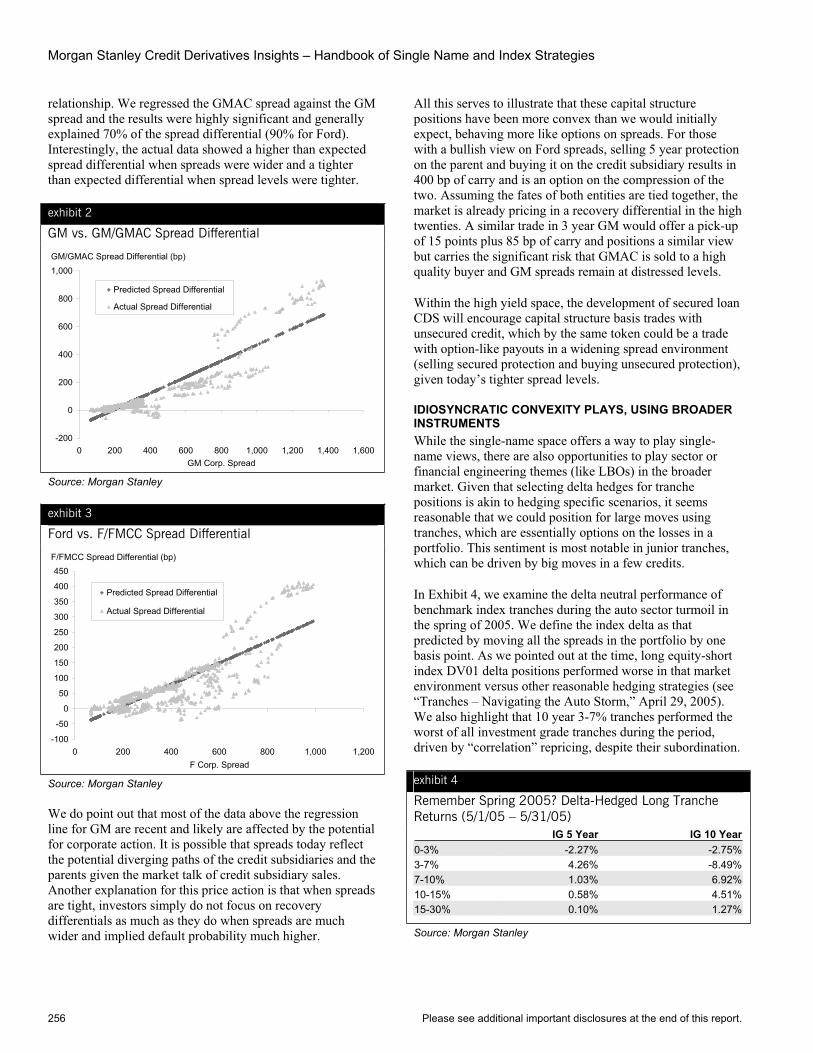
Morgan Stanley Credit Derivatives Insights – Handbook of Single Name and Index Strategies
256 Please see additional important disclosures at the end of this report.
relationship. We regressed the GMAC spread against the GM spread and the results were highly significant and generally explained 70% of the spread differential (90% for Ford). Interestingly, the actual data showed a higher than expected spread differential when spreads were wider and a tighter than expected differential when spread levels were tighter.
exhibit 2
GM vs. GM/GMAC Spread Differential
GM/GMAC Spread Differential (bp)
-200
0
200
400
600
800
1,000
0 200 400 600 800 1,000 1,200 1,400 1,600GM Corp. Spread
Predicted Spread Differential
Actual Spread Differential
Source: Morgan Stanley
exhibit 3
Ford vs. F/FMCC Spread Differential
F/FMCC Spread Differential (bp)
-100
-50
0
50
100
150
200
250
300
350
400
450
0 200 400 600 800 1,000 1,200F Corp. Spread
Predicted Spread Differential
Actual Spread Differential
Source: Morgan Stanley
We do point out that most of the data above the regression line for GM are recent and likely are affected by the potential for corporate action. It is possible that spreads today reflect the potential diverging paths of the credit subsidiaries and the parents given the market talk of credit subsidiary sales. Another explanation for this price action is that when spreads are tight, investors simply do not focus on recovery differentials as much as they do when spreads are much wider and implied default probability much higher.
All this serves to illustrate that these capital structure positions have been more convex than we would initially expect, behaving more like options on spreads. For those with a bullish view on Ford spreads, selling 5 year protection on the parent and buying it on the credit subsidiary results in 400 bp of carry and is an option on the compression of the two. Assuming the fates of both entities are tied together, the market is already pricing in a recovery differential in the high twenties. A similar trade in 3 year GM would offer a pick-up of 15 points plus 85 bp of carry and positions a similar view but carries the significant risk that GMAC is sold to a high quality buyer and GM spreads remain at distressed levels.
Within the high yield space, the development of secured loan CDS will encourage capital structure basis trades with unsecured credit, which by the same token could be a trade with option-like payouts in a widening spread environment (selling secured protection and buying unsecured protection), given today’s tighter spread levels.
IDIOSYNCRATIC CONVEXITY PLAYS, USING BROADER INSTRUMENTSWhile the single-name space offers a way to play single-name views, there are also opportunities to play sector or financial engineering themes (like LBOs) in the broader market. Given that selecting delta hedges for tranche positions is akin to hedging specific scenarios, it seems reasonable that we could position for large moves using tranches, which are essentially options on the losses in a portfolio. This sentiment is most notable in junior tranches, which can be driven by big moves in a few credits.
In Exhibit 4, we examine the delta neutral performance of benchmark index tranches during the auto sector turmoil in the spring of 2005. We define the index delta as that predicted by moving all the spreads in the portfolio by one basis point. As we pointed out at the time, long equity-short index DV01 delta positions performed worse in that market environment versus other reasonable hedging strategies (see “Tranches – Navigating the Auto Storm,” April 29, 2005). We also highlight that 10 year 3-7% tranches performed the worst of all investment grade tranches during the period, driven by “correlation” repricing, despite their subordination.
exhibit 4
Remember Spring 2005? Delta-Hedged Long Tranche Returns (5/1/05 – 5/31/05) IG 5 Year IG 10 Year0-3% -2.27% -2.75%3-7% 4.26% -8.49%7-10% 1.03% 6.92%10-15% 0.58% 4.51%15-30% 0.10% 1.27%
Source: Morgan Stanley

Section E, Chapter 64 So Much Convexity, So Few Options
Please see additional important disclosures at the end of this report. 257
While the events at the time were exacerbated by market technicals, it seems reasonable to assume that in a similar market environment being short equity or equity like mezzanine tranches versus a DV01 index delta is equivalent to buying options on a concentrated set of names widening rather dramatically. In May of 2005 it was the auto names in CDX 3 and 4, but in 2006 the driver could be a widening in the LBO names present in CDX 5, or, in fact, big moves in the auto names in the off-the-run indices. We do caution that general tranche market sentiment could reduce or enhance the performance of these strategies as it effectively imbeds an implied correlation view.
ARE OPTIONS A REAL OPTION? While we have spent the bulk of our effort in this chapter trying to devise investment strategies that have option-like qualities, it is probably worth exploring a real options solution as well. The CDX HiVol index comprises 30 names, and series 4 has auto exposure while series 5 has LBO exposure. Buying options to buy and sell protection on HiVol (a straddle or better yet a strangle if one can find OTM quotes) is a natural strategy to implement convexity views, and positive payouts can happen for medium-sized moves in spread for the names in question. Yet, at implied volatilities near 40% (similar for iTraxx HiVol), this volatility play is not necessarily cheap. We estimate that positioning a short view in CDX HiVol 4 costs approximately 50% more for 5 months in spread options than in the index directly (while protecting yourself from the downside of credit tightening). Whether this is worth it depends on one’s view of how extreme the spread moves will be, but it amounts to an additional 11 bp of widening on the underlying index to break even on the trade. If we assume a move is concentrated in the auto names, this maps to about 80 bp of spread widening for each of the 4 auto names.
exhibit 5
HiVol Options Are Not Cheap
Return (%)
-4.0%
-2.0%
0.0%
2.0%
4.0%
6.0%
8.0%
25 50 75 100 125 150 175 200 225 250 275 300Index Spread
Index Position Option Position
Source: Morgan Stanley
SINGLE-NAME OPTIONS MARKETS – WALK BEFORE YOU CAN RUN Finally, a word on the single-name options market seems appropriate at this point. As we said at the outset, a well-developed market would make credit convexity plays much simpler, but we are not there yet for a variety of reasons. Risk-managing a single-name option is much more difficult than an index option, mainly because of the increased likelihood of jump risk in one name versus a large portfolio of names. This jump risk makes typical distributions (which are important parts of options pricing models) much less relevant. There are “jump-diffusion” models out there, but even with those, the risk-management issues remain.
While the development of an index option market is a necessary first step, even a well-developed index option market is not enough to jump-start (no pun, again) single-name options – but we remain hopeful, despite the structural issues that have hampered the development to date.
In absence of an options market, the most relevant approaches are the debt capital structure basis opportunities (which are arguably limited in investment grade and still developing in high yield), and delta-hedged equity tranche protection strategies.

Morgan Stanley Credit Derivatives Insights – Handbook of Single Name and Index Strategies
258 Please see additional important disclosures at the end of this report.
Chapter 65
Volatility Gets Technical Too December 8, 2006
Primary Analyst: Sivan Mahadevan Primary Analyst: Pinar Onur Primary Analyst: Andrew Sheets Primary Analyst: Phanikiran Naraparaju
Innovation is certainly a key theme in the market today, much to some investors’ collective chagrin. There are some clear common elements in this innovation, including structures rated to market risk, principal protected structures, and synthetic products that require third-party management. But one not-so-subtle common thread that we see is the innovation in optionality. Many products and ideas are indirectly creating an often complicated series of options on spreads in an attempt to get the types of returns that investors desire in today’s markets. One offshoot of this innovation is that it may ultimately help to deepen a spread options market that many, ourselves included, would welcome (see Chapter 9).
For now, we only have an option market in on-the-run iTraxx and CDX indices, and despite three years of activity, expiries remain relatively short-dated in nature, even though many investors would like to see longer-dated options trade. Liquidity and volume have been improving, particularly in Europe. There is also limited activity on options on index tranches. Hedging is certainly an issue, and even in the much more mature equity options markets, we do not see a tremendous amount of liquidity in long-dated options (> 1 year) on the popular equity market indices.
An important theme over the second half of 2006 is the decline in volatility across markets. Credit has been no different – realized volatility has consistently underperformed expectations since summer ended. The drop in volatility is attracting investors looking for spread convexity and fuelling structured products explicitly taking a view on volatility, such as range accrual and CPDO. On the other hand many trades are implicitly becoming correlated to volatility. As real-world default risk remains low, the risk-premium compression is driving many trades.
In the backdrop of a low volatility environment, index options in Europe have been steadily increasing in breadth and depth. Monthly volumes (notional) for iTraxx XOver S6 options, is upwards of 13 billion, by one estimate. There is also a broader investor base getting involved – while hedge funds have been active in this space, we see at least some traditional credit investors, including high yield funds and loan portfolios, getting comfortable expressing views using options. The availability of options on different indices in Europe (XOver,
HiVol and Main), and option expiries (typically between one and six months) makes for interesting opportunities.
• CDS option specifications include: (a) the underlying CDS, usually 5yr maturity; (b) type of option (payer or receiver – see below); (c) strike level specified for the spread (typical range 90–130% of current spread); and (d) option expiry (typical range 1–6 months).
• The options are European, and exercisable only on expiry date. The option price, quoted in bp, is paid up front. No other cash flows are exchanged till the expiry.
• A payer option gives the right to buy a fixed notional of CDS protection (i.e., pay CDS premium) at a fixed spread level, on a fixed date.
• A receiver option gives the right to sell a fixed notional of CDS protection (i.e., receive CDS premium), at a fixed spread level, on a fixed date.
DIFFERING INDEX TECHNICALS Given that liquidity in the credit options market remains focused on the indices, one important market theme is that the CPDO-related flow and speculation, which are centered on the 5-year iTraxx 6 Main and CDX IG 7 indices, have resulted in a jump in implied volatility on these indices versus riskier XOver options. While such a volatility difference is generally not intuitive, it is justified given potential flows on the indices and roll dates. Investment strategies will need to consider the details of option expiry and CPDO roll windows.
exhibit 1
Credit Volatilities Diverge
0%
10%
20%
30%
40%
50%
60%
Nov-05 Jan-06 Mar-06 May-06 Jul-06 Sep-06 Nov-06
Xover HiVol IG Implied Volatility (3m Xover Index)
Note: 1month Realized Volatility Source: Morgan Stanley, Bloomberg
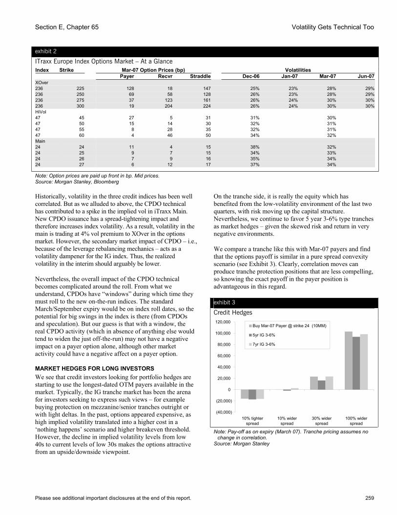
Section E, Chapter 65 Volatility Gets Technical Too
Please see additional important disclosures at the end of this report. 259
exhibit 2
ITraxx Europe Index Options Market – At a Glance Index Strike Mar-07 Option Prices (bp) Volatilities Payer Recvr Straddle Dec-06 Jan-07 Mar-07 Jun-07XOver 236 225 128 18 147 25% 23% 28% 29%236 250 69 58 128 26% 23% 28% 29%236 275 37 123 161 26% 24% 30% 30%236 300 19 204 224 26% 24% 30% 30%HiVol 47 45 27 5 31 31% 30% 47 50 15 14 30 32% 31% 47 55 8 28 35 32% 31% 47 60 4 46 50 34% 32% Main24 24 11 4 15 38% 32%24 25 9 7 15 34% 33%24 26 7 9 16 35% 34%24 27 6 12 17 37% 34%
Note: Option prices are paid up front in bp. Mid prices. Source: Morgan Stanley, Bloomberg
Historically, volatility in the three credit indices has been well correlated. But as we alluded to above, the CPDO technical has contributed to a spike in the implied vol in iTraxx Main. New CPDO issuance has a spread-tightening impact and therefore increases index volatility. As a result, volatility in the main is trading at 4% vol premium to XOver in the options market. However, the secondary market impact of CPDO – i.e., because of the leverage rebalancing mechanics – acts as a volatility dampener for the IG index. Thus, the realized volatility in the interim should arguably be lower.
Nevertheless, the overall impact of the CPDO technical becomes complicated around the roll. From what we understand, CPDOs have “windows” during which time they must roll to the new on-the-run indices. The standard March/September expiry would be on index roll dates, so the potential for big swings in the index is there (from CPDOs and speculation). But our guess is that with a window, the real CPDO activity (which in absence of anything else would tend to widen the just off-the-run) may not have a negative impact on a payer option alone, although other market activity could have a negative affect on a payer option.
MARKET HEDGES FOR LONG INVESTORS We see that credit investors looking for portfolio hedges are starting to use the longest-dated OTM payers available in the market. Typically, the IG tranche market has been the arena for investors seeking to express such views – for example buying protection on mezzanine/senior tranches outright or with light deltas. In the past, options appeared expensive, as high implied volatility translated into a higher cost in a ‘nothing happens’ scenario and higher breakeven threshold. However, the decline in implied volatility levels from low 40s to current levels of low 30s makes the options attractive from an upside/downside viewpoint.
On the tranche side, it is really the equity which has benefited from the low-volatility environment of the last two quarters, with risk moving up the capital structure. Nevertheless, we continue to favor 5 year 3-6% type tranches as market hedges – given the skewed risk and return in very negative environments.
We compare a tranche like this with Mar-07 payers and find that the options payoff is similar in a pure spread convexity scenario (see Exhibit 3). Clearly, correlation moves can produce tranche protection positions that are less compelling, so knowing the exact payoff in the payer position is advantageous in this regard.
exhibit 3
Credit Hedges
(40,000)
(20,000)
0
20,000
40,000
60,000
80,000
100,000
120,000
10% tighterspread
10% widerspread
30% widerspread
100% widerspread
Buy Mar-07 Payer @ strike 24 (10MM)
5yr IG 3-6%
7yr IG 3-6%
Note: Pay-off as on expiry (March 07). Tranche pricing assumes no change in correlation.
Source: Morgan Stanley

Morgan Stanley Credit Derivatives Insights – Handbook of Single Name and Index Strategies
260 Please see additional important disclosures at the end of this report.
YIELD ENHANCEMENT STRATEGY FOR SHORT INVESTORSWe also find the term structure of volatility very interesting in iTraxx XOver. Selling short-dated volatility has always been a popular trade – December and January volatility have steadily traded about 5 volatility points lower in the last month or so. As a result, March expiry is priced at almost 6 volatility points higher than the January expiry. On the other hand, the curve between March and June remains quite flat. We have seen in the past that the post-roll environment translates into a higher level of volatility. From a yield-enhancement point of view, selling volatility seems to be the most attractive in the March maturity in the XOver index. The time decay over a one-month time for the March expiry is worth 1.5 vol points higher than for the June option. Thus, in an environment where the index remains fairly range-bound, the March option will help enhance yield. We believe there will be increased focus on the June expiry in early 2007. Until then, investors who are long protection in XOver can improve the breakevens and positioning for a modest widening in spreads by selling OTM March-07 payers at 275 bp strike. The payoff for the net position gets capped in extreme spread-widening scenarios.
exhibit 4
Yield Enhancement for Short Investors
(150,000)
(100,000)
(50,000)
-
50,000
100,000
150,000
200,000
250,000
210 220 230 240 250 260 270 280 290
Sell Payer - Mar-07 @ 275
Short Market
Net Position
Note: 10MM Notional position in the index and the option Source: Morgan Stanley
CONCLUSION – VOLATILITY GETS TECHNICAL Market participants continue to ask for a wide variety of volatility products, but it has been difficult for the market to deliver, given hedging issues and the like. For now, we continue to have near-dated options on the indices, and liquidity and market depth appear to be improving, at least in Europe. At today’s general volatility levels, index options have become interesting hedging tools relative to some other alternatives. But they are not without technicals, thanks in part to the CPDO phenomenon.
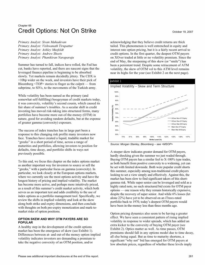
Please see additional important disclosures at the end of this report. 261
Chapter 66
Credit Options: Not On Strike October 19, 2007
Primary Analyst: Sivan Mahadevan Primary Analyst: Vishwanath Tirupattur Primary Analyst: Ashley Musfeldt Primary Analyst: Andrew Sheets Primary Analyst: Phanikiran Naraparaju
Summer has turned to fall, indices have rolled, the Fed has cut, banks have reported, and there are nascent signs that the leveraged finance pipeline is beginning to be absorbed slowly. Yet markets remain decidedly jittery. The CDX is +10bp wider on the week, and investors have their pick of Bloomberg <TOP> stories to finger as the culprit — from subprime, to SIVs, to the movements of the Turkish army.
While volatility has been named as the primary (and somewhat self-fulfilling) boogeyman of credit markets today, it was convexity, volatility’s second cousin, which caused its fair share of summer’s troubles. As a secular shift in credit investing has moved risk-taking into structured forms, many portfolios have become more out-of-the-money (OTM) in nature, good for avoiding random defaults, but at the expense of greater gamma (convexity) exposure.
The success of index tranches has in large part been a response to this changing risk profile many investors now face. Tranches have created a liquid, tradable market for “greeks” in a short period of time, across a range of maturities and portfolios, allowing investors to position for defaults, time decay, and portfolio shifts in ways not previously possible.
To this end, we focus this chapter on the index options market as another important way for investors to source or sell the “greeks,” with a particular focus on gamma (convexity). In particular, we look closely at the European options markets, where we currently see the most options activity and have the longest history of pricing and implied volatility. The market has become more active, and perhaps more intuitively priced, as a result of this summer’s credit market activity, which both serves as an important test and adds credibility to the use of index options as a portfolio management tool. Specifically, we review the shifts in implied volatility and look at the skew along both strike and expiry dimensions, and then conclude with thoughts on both pre-expiry monetization and mark-to-market risks of option positions.
OPTION SKEW AND WHY OTM PAYERS ARE SO POPULAR A healthy step in the development of the credit options market has been the emergence of skew (see Exhibit 1). Differences between at- and out-of-the money option implied volatility indicates investors are demanding a premium to take the negative convexity of an OTM position, and/or
acknowledging that they believe credit returns are thick tailed. This phenomenon is well entrenched in equity and interest rate option pricing, but it is a fairly recent arrival to credit options. In the first quarter, the deepest OTM payers on XOver traded at little or no volatility premium. Since the end of May, the steepening of this skew (or “smile”) has been a persistent trend. Despite some retracement of ATM volatility, the skew of OTM vol to this ATM level remains near its highs for the year (see Exhibit 2 on the next page).
exhibit 1
Implied Volatility – Skew and Term Structure
50%
55%
60%
65%
70%
75%
80%
85%
90%
95%
100%
73% 81% 90% 98% 106% 114% 122% 130% 138% 147%
Strike Level (%)
Impl
ied
Vola
tility
(%)
XOver Nov-07 Expiry
XOver Dec-07 Expiry
XOver Mar-08 Expiry
Main Dec-07 Expiry
Main Mar-08 Expiry
Source: Morgan Stanley, Bloomberg – see <MSOP>
A steeper skew indicates greater demand for OTM payers, hardly shocking given the summer we just waded through. Buying OTM payers has a similar feel to X-100% type trades, as both benefit from positive convexity to a widening, yet can be set with limited downside. Both were popular credit shorts this summer, especially among non-traditional credit players looking to set a view simply and effectively. Against this, the market has been slow to find significant takers of this short-gamma risk. While super senior can be leveraged and sold as a highly rated note, no such structured bid exists for OTM payer options — one reason why they remain historically expensive, despite the recovery of super senior. And while 6% losses (let alone 22%) have yet to be observed on an iTraxx-rated portfolio back to 1970, today’s deepest OTM payers would have been in-the-money less than three months ago.
Option pricing dynamics also seem to be having a greater effect. We have seen a consistent pattern of rising implied volatility in response to wider spreads, which has added an extra kicker to the convexity of buying OTM payer (see Exhibit 2). Optics matter as well. As time passes, OTM premiums should fall in any options model due to time decay, all else being equal. But as time to maturity shortens, a significant “why not” bid has emerged for OTM payers at low absolute prices, regardless of whether these levels imply
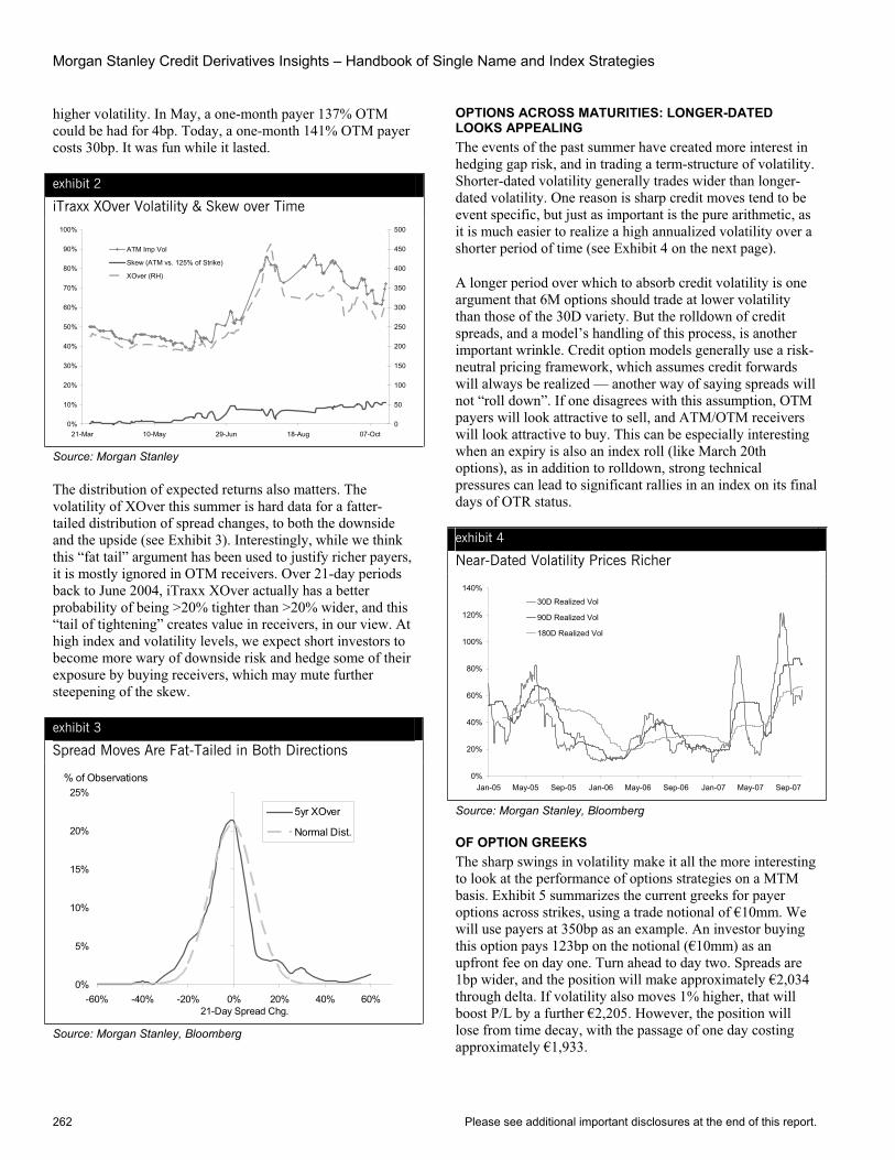
Morgan Stanley Credit Derivatives Insights – Handbook of Single Name and Index Strategies
262 Please see additional important disclosures at the end of this report.
higher volatility. In May, a one-month payer 137% OTM could be had for 4bp. Today, a one-month 141% OTM payer costs 30bp. It was fun while it lasted.
exhibit 2
iTraxx XOver Volatility & Skew over Time
0%
10%
20%
30%
40%
50%
60%
70%
80%
90%
100%
21-Mar 10-May 29-Jun 18-Aug 07-Oct0
50
100
150
200
250
300
350
400
450
500
ATM Imp Vol
Skew (ATM vs. 125% of Strike)
XOver (RH)
Source: Morgan Stanley
The distribution of expected returns also matters. The volatility of XOver this summer is hard data for a fatter-tailed distribution of spread changes, to both the downside and the upside (see Exhibit 3). Interestingly, while we think this “fat tail” argument has been used to justify richer payers, it is mostly ignored in OTM receivers. Over 21-day periods back to June 2004, iTraxx XOver actually has a better probability of being >20% tighter than >20% wider, and this “tail of tightening” creates value in receivers, in our view. At high index and volatility levels, we expect short investors to become more wary of downside risk and hedge some of their exposure by buying receivers, which may mute further steepening of the skew.
exhibit 3
Spread Moves Are Fat-Tailed in Both Directions
% of Observations
0%
5%
10%
15%
20%
25%
-60% -40% -20% 0% 20% 40% 60%21-Day Spread Chg.
5yr XOver
Normal Dist.
Source: Morgan Stanley, Bloomberg
OPTIONS ACROSS MATURITIES: LONGER-DATED LOOKS APPEALING The events of the past summer have created more interest in hedging gap risk, and in trading a term-structure of volatility. Shorter-dated volatility generally trades wider than longer-dated volatility. One reason is sharp credit moves tend to be event specific, but just as important is the pure arithmetic, as it is much easier to realize a high annualized volatility over a shorter period of time (see Exhibit 4 on the next page).
A longer period over which to absorb credit volatility is one argument that 6M options should trade at lower volatility than those of the 30D variety. But the rolldown of credit spreads, and a model’s handling of this process, is another important wrinkle. Credit option models generally use a risk-neutral pricing framework, which assumes credit forwards will always be realized — another way of saying spreads will not “roll down”. If one disagrees with this assumption, OTM payers will look attractive to sell, and ATM/OTM receivers will look attractive to buy. This can be especially interesting when an expiry is also an index roll (like March 20th options), as in addition to rolldown, strong technical pressures can lead to significant rallies in an index on its final days of OTR status.
exhibit 4
Near-Dated Volatility Prices Richer
0%
20%
40%
60%
80%
100%
120%
140%
Jan-05 May-05 Sep-05 Jan-06 May-06 Sep-06 Jan-07 May-07 Sep-07
30D Realized Vol
90D Realized Vol
180D Realized Vol
Source: Morgan Stanley, Bloomberg
OF OPTION GREEKS The sharp swings in volatility make it all the more interesting to look at the performance of options strategies on a MTM basis. Exhibit 5 summarizes the current greeks for payer options across strikes, using a trade notional of €10mm. We will use payers at 350bp as an example. An investor buying this option pays 123bp on the notional (€10mm) as an upfront fee on day one. Turn ahead to day two. Spreads are 1bp wider, and the position will make approximately €2,034 through delta. If volatility also moves 1% higher, that will boost P/L by a further €2,205. However, the position will lose from time decay, with the passage of one day costing approximately €1,933.
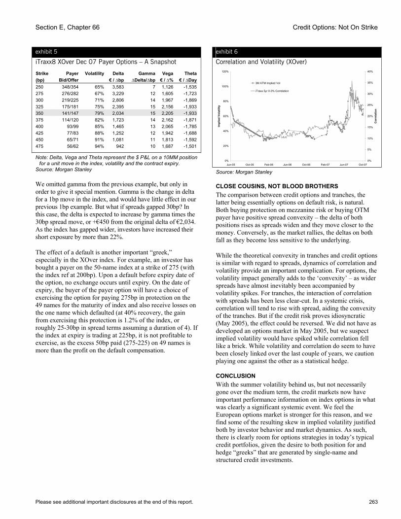
Section E, Chapter 66 Credit Options: Not On Strike
Please see additional important disclosures at the end of this report. 263
exhibit 5
iTraxx8 XOver Dec 07 Payer Options – A Snapshot
Strike Payer Volatility Delta Gamma Vega Theta(bp) Bid/Offer € / bp Delta/ bp € / % € / Day250 348/354 65% 3,583 7 1,126 -1,535275 276/282 67% 3,229 12 1,605 -1,723300 219/225 71% 2,806 14 1,967 -1,869325 175/181 75% 2,395 15 2,156 -1,933350 141/147 79% 2,034 15 2,205 -1,933375 114/120 82% 1,723 14 2,162 -1,871400 93/99 85% 1,465 13 2,065 -1,785425 77/83 88% 1,252 12 1,942 -1,688450 65/71 91% 1,081 11 1,813 -1,592475 56/62 94% 942 10 1,687 -1,501
Note: Delta, Vega and Theta represent the $ P&L on a 10MM position for a unit move in the index, volatility and the contract expiry.
Source: Morgan Stanley
We omitted gamma from the previous example, but only in order to give it special mention. Gamma is the change in delta for a 1bp move in the index, and would have little effect in our previous 1bp example. But what if spreads gapped 30bp? In this case, the delta is expected to increase by gamma times the 30bp spread move, or +€450 from the original delta of €2,034. As the index has gapped wider, investors have increased their short exposure by more than 22%.
The effect of a default is another important “greek,” especially in the XOver index. For example, an investor has bought a payer on the 50-name index at a strike of 275 (with the index ref at 200bp). Upon a default before expiry date of the option, no exchange occurs until expiry. On the date of expiry, the buyer of the payer option will have a choice of exercising the option for paying 275bp in protection on the 49 names for the maturity of index and also receive losses on the one name which defaulted (at 40% recovery, the gain from exercising this protection is 1.2% of the index, or roughly 25-30bp in spread terms assuming a duration of 4). If the index at expiry is trading at 225bp, it is not profitable to exercise, as the excess 50bp paid (275-225) on 49 names is more than the profit on the default compensation.
exhibit 6
Correlation and Volatility (XOver)
0%
20%
40%
60%
80%
100%
120%
Jun-05 Oct-05 Feb-06 Jun-06 Oct-06 Feb-07 Jun-07 Oct-07
Impl
ied
Vola
tility
0%
5%
10%
15%
20%
25%
30%
35%
40%
Cor
rela
tion
3M ATM Implied Vol
iTraxx 5yr 0-3% Correlation
Source: Morgan Stanley
CLOSE COUSINS, NOT BLOOD BROTHERS The comparison between credit options and tranches, the latter being essentially options on default risk, is natural. Both buying protection on mezzanine risk or buying OTM payer have positive spread convexity – the delta of both positions rises as spreads widen and they move closer to the money. Conversely, as the market rallies, the deltas on both fall as they become less sensitive to the underlying.
While the theoretical convexity in tranches and credit options is similar with regard to spreads, dynamics of correlation and volatility provide an important complication. For options, the volatility impact generally adds to the ‘convexity’ – as wider spreads have almost inevitably been accompanied by volatility spikes. For tranches, the interaction of correlation with spreads has been less clear-cut. In a systemic crisis, correlation will tend to rise with spread, aiding the convexity of the tranches. But if the credit risk proves idiosyncratic (May 2005), the effect could be reversed. We did not have as developed an options market in May 2005, but we suspect implied volatility would have spiked while correlation fell like a brick. While volatility and correlation do seem to have been closely linked over the last couple of years, we caution playing one against the other as a statistical hedge.
CONCLUSIONWith the summer volatility behind us, but not necessarily gone over the medium term, the credit markets now have important performance information on index options in what was clearly a significant systemic event. We feel the European options market is stronger for this reason, and we find some of the resulting skew in implied volatility justified both by investor behavior and market dynamics. As such, there is clearly room for options strategies in today’s typical credit portfolios, given the desire to both position for and hedge “greeks” that are generated by single-name and structured credit investments.
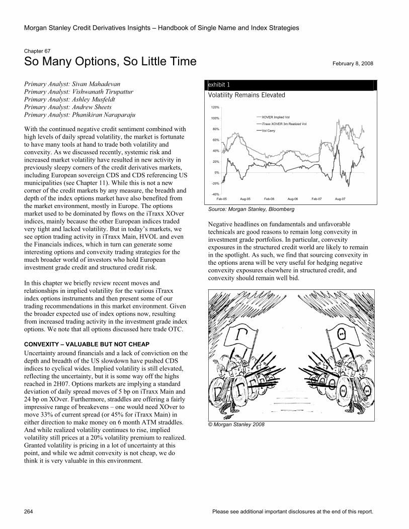
Morgan Stanley Credit Derivatives Insights – Handbook of Single Name and Index Strategies
264 Please see additional important disclosures at the end of this report.
Chapter 67
So Many Options, So Little Time February 8, 2008
Primary Analyst: Sivan Mahadevan Primary Analyst: Vishwanath Tirupattur Primary Analyst: Ashley Musfeldt Primary Analyst: Andrew Sheets Primary Analyst: Phanikiran Naraparaju
With the continued negative credit sentiment combined with high levels of daily spread volatility, the market is fortunate to have many tools at hand to trade both volatility and convexity. As we discussed recently, systemic risk and increased market volatility have resulted in new activity in previously sleepy corners of the credit derivatives markets, including European sovereign CDS and CDS referencing US municipalities (see Chapter 11). While this is not a new corner of the credit markets by any measure, the breadth and depth of the index options market have also benefited from the market environment, mostly in Europe. The options market used to be dominated by flows on the iTraxx XOver indices, mainly because the other European indices traded very tight and lacked volatility. But in today’s markets, we see option trading activity in iTraxx Main, HVOL and even the Financials indices, which in turn can generate some interesting options and convexity trading strategies for the much broader world of investors who hold European investment grade credit and structured credit risk.
In this chapter we briefly review recent moves and relationships in implied volatility for the various iTraxx index options instruments and then present some of our trading recommendations in this market environment. Given the broader expected use of index options now, resulting from increased trading activity in the investment grade index options. We note that all options discussed here trade OTC.
CONVEXITY – VALUABLE BUT NOT CHEAP Uncertainty around financials and a lack of conviction on the depth and breadth of the US slowdown have pushed CDS indices to cyclical wides. Implied volatility is still elevated, reflecting the uncertainty, but it is some way off the highs reached in 2H07. Options markets are implying a standard deviation of daily spread moves of 5 bp on iTraxx Main and 24 bp on XOver. Furthermore, straddles are offering a fairly impressive range of breakevens – one would need XOver to move 33% of current spread (or 45% for iTraxx Main) in either direction to make money on 6 month ATM straddles. And while realized volatility continues to rise, implied volatility still prices at a 20% volatility premium to realized. Granted volatility is pricing in a lot of uncertainty at this point, and while we admit convexity is not cheap, we do think it is very valuable in this environment.
exhibit 1
Volatility Remains Elevated
-40%
-20%
0%
20%
40%
60%
80%
100%
120%
Feb-05 Aug-05 Feb-06 Aug-06 Feb-07 Aug-07
XOVER Implied Vol
iTraxx XOVER 3m Realized Vol
Vol Carry
Source: Morgan Stanley, Bloomberg
Negative headlines on fundamentals and unfavorable technicals are good reasons to remain long convexity in investment grade portfolios. In particular, convexity exposures in the structured credit world are likely to remain in the spotlight. As such, we find that sourcing convexity in the options arena will be very useful for hedging negative convexity exposures elsewhere in structured credit, and convexity should remain well bid.
© Morgan Stanley 2008
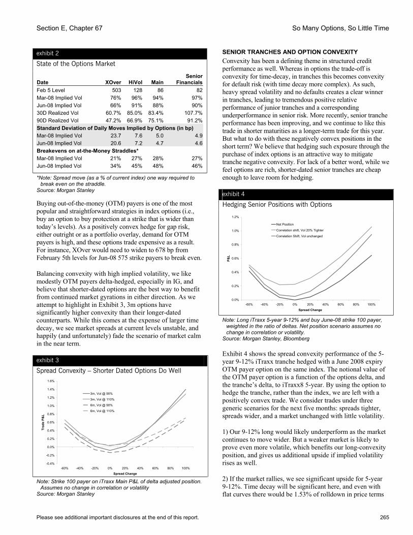
Section E, Chapter 67 So Many Options, So Little Time
Please see additional important disclosures at the end of this report. 265
exhibit 2
State of the Options Market
Date XOver HiVol Main Senior
FinancialsFeb 5 Level 503 128 86 82Mar-08 Implied Vol 76% 96% 94% 97%Jun-08 Implied Vol 66% 91% 88% 90%30D Realized Vol 60.7% 85.0% 83.4% 107.7%90D Realized Vol 47.2% 66.9% 75.1% 91.2%Standard Deviation of Daily Moves Implied by Options (in bp) Mar-08 Implied Vol 23.7 7.6 5.0 4.9Jun-08 Implied Vol 20.6 7.2 4.7 4.6Breakevens on at-the-Money Straddles* Mar-08 Implied Vol 21% 27% 28% 27%Jun-08 Implied Vol 34% 45% 48% 46%
*Note: Spread move (as a % of current index) one way required to break even on the straddle.
Source: Morgan Stanley
Buying out-of-the-money (OTM) payers is one of the most popular and straightforward strategies in index options (i.e., buy an option to buy protection at a strike that is wider than today’s levels). As a positively convex hedge for gap risk, either outright or as a portfolio overlay, demand for OTM payers is high, and these options trade expensive as a result. For instance, XOver would need to widen to 678 bp from February 5th levels for Jun-08 575 strike payers to break even.
Balancing convexity with high implied volatility, we like modestly OTM payers delta-hedged, especially in IG, and believe that shorter-dated options are the best way to benefit from continued market gyrations in either direction. As we attempt to highlight in Exhibit 3, 3m options have significantly higher convexity than their longer-dated counterparts. While this comes at the expense of larger time decay, we see market spreads at current levels unstable, and happily (and unfortunately) fade the scenario of market calm in the near term.
exhibit 3
Spread Convexity – Shorter Dated Options Do Well
-0.4%
-0.2%
0.0%
0.2%
0.4%
0.6%
0.8%
1.0%
1.2%
1.4%
1.6%
-60% -40% -20% 0% 20% 40% 60% 80% 100%
Spread Change
Trad
e P&
L
3m, Vol @ 90%
3m, Vol @ 110%
6m, Vol @ 90%
6m, Vol @ 110%
Note: Strike 100 payer on iTraxx Main P&L of delta adjusted position. Assumes no change in correlation or volatility
Source: Morgan Stanley
SENIOR TRANCHES AND OPTION CONVEXITY Convexity has been a defining theme in structured credit performance as well. Whereas in options the trade-off is convexity for time-decay, in tranches this becomes convexity for default risk (with time decay more complex). As such, heavy spread volatility and no defaults creates a clear winner in tranches, leading to tremendous positive relative performance of junior tranches and a corresponding underperformance in senior risk. More recently, senior tranche performance has been improving, and we continue to like this trade in shorter maturities as a longer-term trade for this year. But what to do with these negatively convex positions in the short term? We believe that hedging such exposure through the purchase of index options is an attractive way to mitigate tranche negative convexity. For lack of a better word, while we feel options are rich, shorter-dated senior tranches are cheap enough to leave room for hedging.
exhibit 4
Hedging Senior Positions with Options
0.0%
0.2%
0.4%
0.6%
0.8%
1.0%
1.2%
-60% -40% -20% 0% 20% 40% 60% 80% 100%
Spread Change
P&L
Net Position
Correlation shift, Vol 20% Tighter
Correlation Shift, Vol unchanged
Note: Long iTraxx 5-year 9-12% and buy June-08 strike 100 payer, weighted in the ratio of deltas. Net position scenario assumes no change in correlation or volatility.
Source: Morgan Stanley, Bloomberg
Exhibit 4 shows the spread convexity performance of the 5-year 9-12% iTraxx tranche hedged with a June 2008 expiry OTM payer option on the same index. The notional value of the OTM payer option is a function of the options delta, and the tranche’s delta, to iTraxx8 5-year. By using the option to hedge the tranche, rather than the index, we are left with a positively convex trade. We consider trades under three generic scenarios for the next five months: spreads tighter, spreads wider, and a market unchanged with little volatility.
1) Our 9-12% long would likely underperform as the market continues to move wider. But a weaker market is likely to prove even more volatile, which benefits our long-convexity position, and gives us additional upside if implied volatility rises as well.
2) If the market rallies, we see significant upside for 5-year 9-12%. Time decay will be significant here, and even with flat curves there would be 1.53% of rolldown in price terms
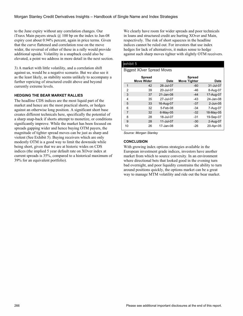
Morgan Stanley Credit Derivatives Insights – Handbook of Single Name and Index Strategies
266 Please see additional important disclosures at the end of this report.
to the June expiry without any correlation changes. Our iTraxx Main payers struck @ 100 bp on the index to Jun-08 expiry cost about 0.94% percent, again in price terms. Given that the curve flattened and correlation rose on the move wider, the reversal of either of these in a rally would provide additional upside. Volatility in a snapback could also be elevated, a point we address in more detail in the next section.
3) A market with little volatility, and a correlation shift against us, would be a negative scenario. But we also see it as the least likely, as stability seems unlikely to accompany a further repricing of structured credit above and beyond currently extreme levels.
HEDGING THE BEAR MARKET RALLIES The headline CDS indices are the most liquid part of the market and hence are the most practical shorts, or hedges against an otherwise long position. A significant short base creates different technicals here, specifically the potential of a sharp snap-back if shorts attempt to monetize, or conditions significantly improve. While the market has been focused on spreads gapping wider and hence buying OTM payers, the magnitude of tighter spread moves can be just as sharp and violent (See Exhibit 5). Buying receivers which are only modestly OTM is a good way to limit the downside while being short, given that we are at historic wides on CDS indices (the implied 5 year default rate on XOver index at current spreads is 35%, compared to a historical maximum of 39% for an equivalent portfolio).
We clearly have room for wider spreads and poor technicals in loans and structured credit are hurting XOver and Main, respectively. The risk of short squeezes in the headline indices cannot be ruled out. For investors that use index hedges for lack of alternatives, it makes sense to hedge against such sharp moves tighter with slightly OTM receivers.
exhibit 5
Biggest XOver Spread Moves
SpreadMove Wider Date
SpreadMove Tighter Date
1 42 26-Jul-07 -60 31-Jul-072 39 20-Jul-07 -46 8-Aug-073 37 21-Jan-08 -44 17-Aug-074 35 27-Jul-07 -43 24-Jan-085 33 16-Aug-07 -37 2-Jun-056 32 5-Feb-08 -34 7-Aug-077 32 6-May-05 -32 18-May-058 28 18-Jul-07 -31 19-Sep-079 28 11-Jul-07 -30 2-Aug-07
10 26 17-Jan-08 -26 20-Apr-05
Source: Morgan Stanley
CONCLUSIONWith growing index options strategies available in the European investment grade indices, investors have another market from which to source convexity. In an environment where directional bets that looked good in the evening turn bad overnight, and poor liquidity constrains the ability to turn around positions quickly, the options market can be a great way to manage MTM volatility and ride out the bear market.
Section F
Credit Market Themes

Morgan Stanley Credit Derivatives Insights – Handbook of Single Name and Index Strategies
268 Please see additional important disclosures at the end of this report.
Chapter 68
Manic Compression March 12, 2004
Primary Analyst: Sivan Mahadevan Primary Analyst: Rizwan Hussain Primary Analyst: Peter Polanskyj Anisha Ambardar
As investors have hunted for and eventually reached for yield in this relatively tight spread environment, we find that relative value relationships in many debt capital structures are getting stretched. In particular, there are numerous examples of subordinate paper trading “rich” to seniors, when we compare the likely recovery rate differences with where the debt instruments trade. Rich valuation, though, is a matter of debate, as many investors consider default to be an extremely unlikely event today (certainly more unlikely than implied by market spreads, for example).
In this chapter, we explore the valuation landscape and compression of valuations between senior and subordinated securities that has been left in the wake of the credit rally that started in late 2002. We then examine what effect varying recovery rates have on the appropriate discount at which subordinated securities should trade relative to senior securities. Finally, we suggest that selected structured credit market senior/sub relationships do not look out of line despite movements in the underlying single-name markets.
EXAMINING HOLDCO VERSUS OPCO UTILITY VALUATIONS Over the past year, utility credit investors have become more comfortable with default risk in the sector, as many of the liquidity issues faced by problem credits in the group have been alleviated through revolver, bank line, and commercial paper refinancings and term-outs in the public credit markets. So, with default risk perceptions on the decline, the narrowing difference between holding company and operating company securities (typically closer to assets in bankruptcy, with associated higher recoveries) is a rational outcome. In Exhibit 1, we track the basis between several selected utility holding company and operating company securities, which exhibit a notable valuation compression since experiencing the most distressed levels of October 2002.
exhibit 1
Now Little Differentiation Between Utility HoldCo and OpCo Spread Valuations
(bp)
-100
0
100
200
300
400
500
600
700
800
900
Oct-02 Dec-02 Feb-03 May-03 Jul-03 Oct-03 Dec-03 Mar-04
AEP FE D TEPGN TXU CIN
Source: Morgan Stanley
REACH FOR YIELD IN SUBORDINATED PAPER IN LAST STAGES? Indeed, much has been made of the reach for additional yield down into the high yield market. Our credit strategist, Greg Peters, has opined in the past that the higher-quality portion of the high yield market serves as a fertile investment ground for crossover and “core-plus” investors in an improving default environment, while the middle tier of the high yield market looks relatively fully valued. Furthermore, within the high yield space, there has certainly been a fair amount of compression within capital structures, with subordinated paper performance outpacing senior issues, as we show in Exhibit 2. Admittedly, the data capturing relative senior and subordinated performance is far from complete for the market, but we believe it is at least indicative of the broader trend at work as investors dip down the capital structure in search of yield.
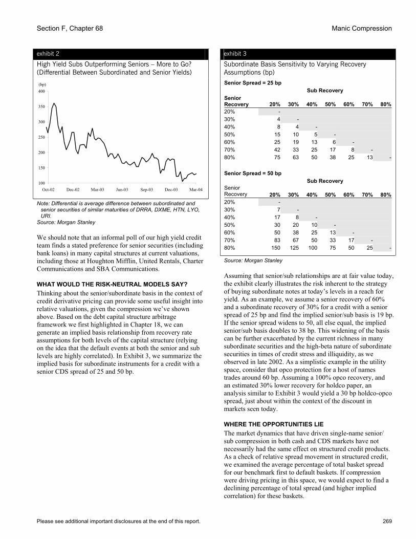
Section F, Chapter 68 Manic Compression
Please see additional important disclosures at the end of this report. 269
exhibit 2
High Yield Subs Outperforming Seniors – More to Go? (Differential Between Subordinated and Senior Yields)
(bp)
100
150
200
250
300
350
400
Oct-02 Dec-02 Mar-03 Jun-03 Sep-03 Dec-03 Mar-04
Note: Differential is average difference between subordinated and senior securities of similar maturities of DRRA, DXME, HTN, LYO, URI.
Source: Morgan Stanley
We should note that an informal poll of our high yield credit team finds a stated preference for senior securities (including bank loans) in many capital structures at current valuations, including those at Houghton Mifflin, United Rentals, Charter Communications and SBA Communications.
WHAT WOULD THE RISK-NEUTRAL MODELS SAY? Thinking about the senior/subordinate basis in the context of credit derivative pricing can provide some useful insight into relative valuations, given the compression we’ve shown above. Based on the debt capital structure arbitrage framework we first highlighted in Chapter 18, we can generate an implied basis relationship from recovery rate assumptions for both levels of the capital structure (relying on the idea that the default events at both the senior and sub levels are highly correlated). In Exhibit 3, we summarize the implied basis for subordinate instruments for a credit with a senior CDS spread of 25 and 50 bp.
exhibit 3
Subordinate Basis Sensitivity to Varying Recovery Assumptions (bp) Senior Spread = 25 bp
Sub Recovery SeniorRecovery 20% 30% 40% 50% 60% 70% 80%20% -30% 4 -40% 8 4 -50% 15 10 5 -60% 25 19 13 6 -70% 42 33 25 17 8 -80% 75 63 50 38 25 13 -
Senior Spread = 50 bp Sub Recovery
SeniorRecovery 20% 30% 40% 50% 60% 70% 80%20% -30% 7 -40% 17 8 -50% 30 20 10 -60% 50 38 25 13 -70% 83 67 50 33 17 -80% 150 125 100 75 50 25 -
Source: Morgan Stanley
Assuming that senior/sub relationships are at fair value today, the exhibit clearly illustrates the risk inherent to the strategy of buying subordinate notes at today’s levels in a reach for yield. As an example, we assume a senior recovery of 60% and a subordinate recovery of 30% for a credit with a senior spread of 25 bp and find the implied senior/sub basis is 19 bp. If the senior spread widens to 50, all else equal, the implied senior/sub basis doubles to 38 bp. This widening of the basis can be further exacerbated by the current richness in many subordinate securities and the high-beta nature of subordinate securities in times of credit stress and illiquidity, as we observed in late 2002. As a simplistic example in the utility space, consider that opco protection for a host of names trades around 60 bp. Assuming a 100% opco recovery, and an estimated 30% lower recovery for holdco paper, an analysis similar to Exhibit 3 would yield a 30 bp holdco-opco spread, just about within the context of the discount in markets seen today.
WHERE THE OPPORTUNITIES LIE The market dynamics that have driven single-name senior/ sub compression in both cash and CDS markets have not necessarily had the same effect on structured credit products. As a check of relative spread movement in structured credit, we examined the average percentage of total basket spread for our benchmark first to default baskets. If compression were driving pricing in this space, we would expect to find a declining percentage of total spread (and higher implied correlation) for these baskets.
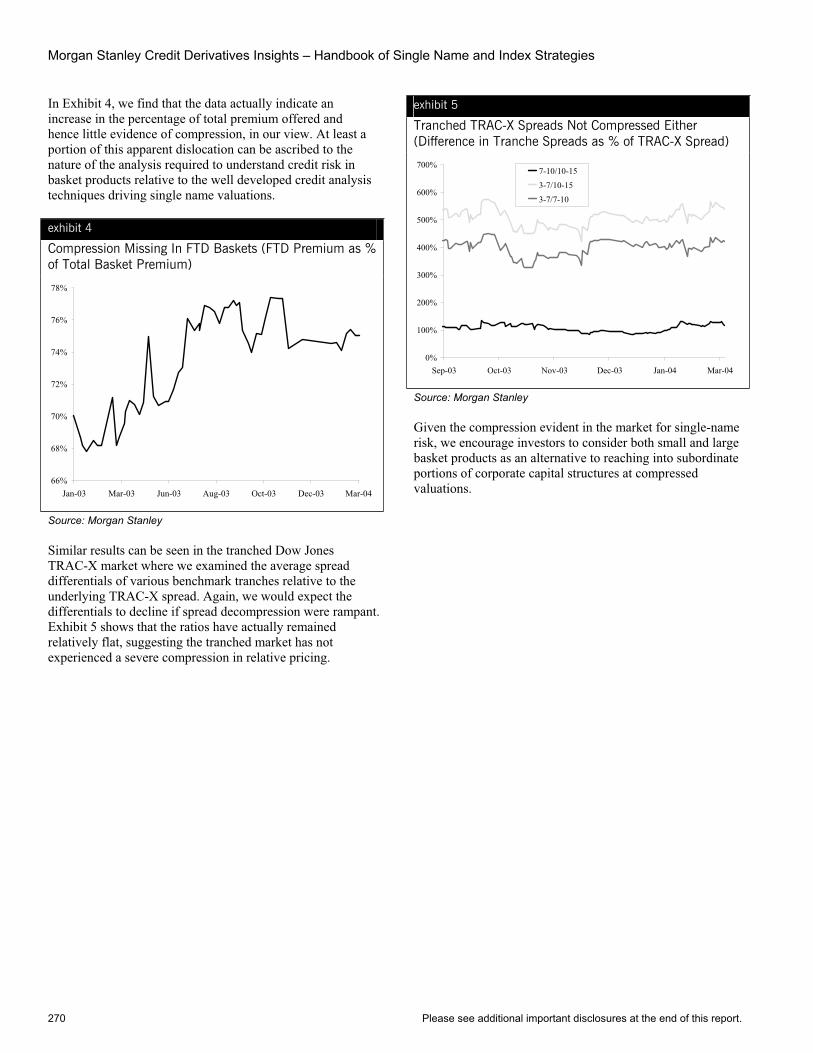
Morgan Stanley Credit Derivatives Insights – Handbook of Single Name and Index Strategies
270 Please see additional important disclosures at the end of this report.
In Exhibit 4, we find that the data actually indicate an increase in the percentage of total premium offered and hence little evidence of compression, in our view. At least a portion of this apparent dislocation can be ascribed to the nature of the analysis required to understand credit risk in basket products relative to the well developed credit analysis techniques driving single name valuations.
exhibit 4
Compression Missing In FTD Baskets (FTD Premium as % of Total Basket Premium)
66%
68%
70%
72%
74%
76%
78%
Jan-03 Mar-03 Jun-03 Aug-03 Oct-03 Dec-03 Mar-04
Source: Morgan Stanley
Similar results can be seen in the tranched Dow Jones TRAC-X market where we examined the average spread differentials of various benchmark tranches relative to the underlying TRAC-X spread. Again, we would expect the differentials to decline if spread decompression were rampant. Exhibit 5 shows that the ratios have actually remained relatively flat, suggesting the tranched market has not experienced a severe compression in relative pricing.
exhibit 5
Tranched TRAC-X Spreads Not Compressed Either (Difference in Tranche Spreads as % of TRAC-X Spread)
0%
100%
200%
300%
400%
500%
600%
700%
Sep-03 Oct-03 Nov-03 Dec-03 Jan-04 Mar-04
7-10/10-15
3-7/10-15
3-7/7-10
Source: Morgan Stanley
Given the compression evident in the market for single-name risk, we encourage investors to consider both small and large basket products as an alternative to reaching into subordinate portions of corporate capital structures at compressed valuations.
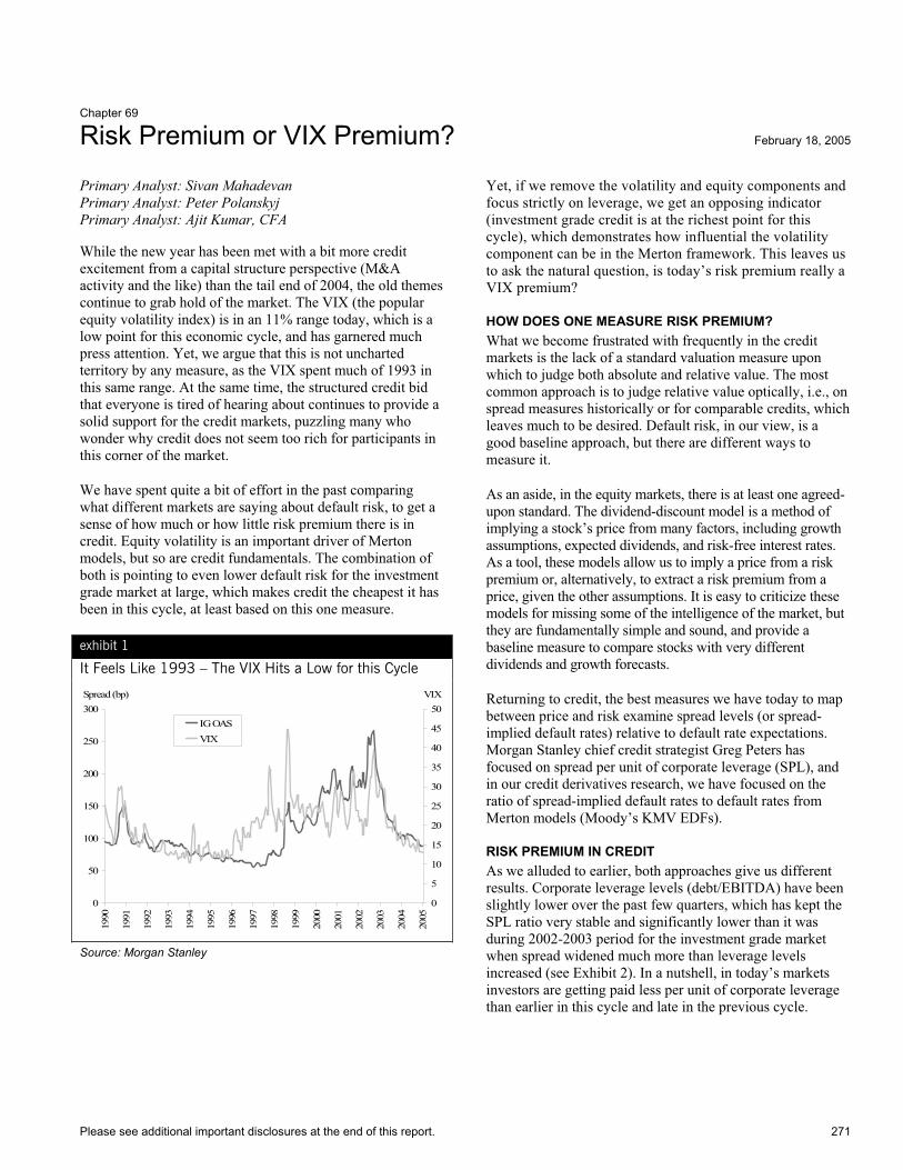
Please see additional important disclosures at the end of this report. 271
Chapter 69
Risk Premium or VIX Premium? February 18, 2005
Primary Analyst: Sivan Mahadevan Primary Analyst: Peter Polanskyj Primary Analyst: Ajit Kumar, CFA
While the new year has been met with a bit more credit excitement from a capital structure perspective (M&A activity and the like) than the tail end of 2004, the old themes continue to grab hold of the market. The VIX (the popular equity volatility index) is in an 11% range today, which is a low point for this economic cycle, and has garnered much press attention. Yet, we argue that this is not uncharted territory by any measure, as the VIX spent much of 1993 in this same range. At the same time, the structured credit bid that everyone is tired of hearing about continues to provide a solid support for the credit markets, puzzling many who wonder why credit does not seem too rich for participants in this corner of the market.
We have spent quite a bit of effort in the past comparing what different markets are saying about default risk, to get a sense of how much or how little risk premium there is in credit. Equity volatility is an important driver of Merton models, but so are credit fundamentals. The combination of both is pointing to even lower default risk for the investment grade market at large, which makes credit the cheapest it has been in this cycle, at least based on this one measure.
exhibit 1
It Feels Like 1993 – The VIX Hits a Low for this Cycle
Spread (bp)
0
50
100
150
200
250
300
1990
1991
1992
1993
1994
1995
1996
1997
1998
1999
2000
2001
2002
2003
2004
2005
0
5
10
15
20
25
30
35
40
45
50VIX
IG OASVIX
Source: Morgan Stanley
Yet, if we remove the volatility and equity components and focus strictly on leverage, we get an opposing indicator (investment grade credit is at the richest point for this cycle), which demonstrates how influential the volatility component can be in the Merton framework. This leaves us to ask the natural question, is today’s risk premium really a VIX premium?
HOW DOES ONE MEASURE RISK PREMIUM? What we become frustrated with frequently in the credit markets is the lack of a standard valuation measure upon which to judge both absolute and relative value. The most common approach is to judge relative value optically, i.e., on spread measures historically or for comparable credits, which leaves much to be desired. Default risk, in our view, is a good baseline approach, but there are different ways to measure it.
As an aside, in the equity markets, there is at least one agreed-upon standard. The dividend-discount model is a method of implying a stock’s price from many factors, including growth assumptions, expected dividends, and risk-free interest rates. As a tool, these models allow us to imply a price from a risk premium or, alternatively, to extract a risk premium from a price, given the other assumptions. It is easy to criticize these models for missing some of the intelligence of the market, but they are fundamentally simple and sound, and provide a baseline measure to compare stocks with very different dividends and growth forecasts.
Returning to credit, the best measures we have today to map between price and risk examine spread levels (or spread-implied default rates) relative to default rate expectations. Morgan Stanley chief credit strategist Greg Peters has focused on spread per unit of corporate leverage (SPL), and in our credit derivatives research, we have focused on the ratio of spread-implied default rates to default rates from Merton models (Moody’s KMV EDFs).
RISK PREMIUM IN CREDIT As we alluded to earlier, both approaches give us different results. Corporate leverage levels (debt/EBITDA) have been slightly lower over the past few quarters, which has kept the SPL ratio very stable and significantly lower than it was during 2002-2003 period for the investment grade market when spread widened much more than leverage levels increased (see Exhibit 2). In a nutshell, in today’s markets investors are getting paid less per unit of corporate leverage than earlier in this cycle and late in the previous cycle.
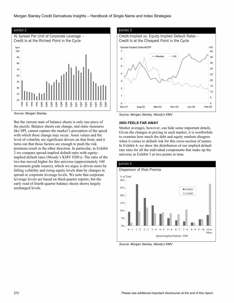
Morgan Stanley Credit Derivatives Insights – Handbook of Single Name and Index Strategies
272 Please see additional important disclosures at the end of this report.
exhibit 2
IG Spread Per Unit of Corporate Leverage – Credit Is at the Richest Point in the Cycle
bp/x
20
30
40
50
60
70
80
90
100
1990
1992
1994
1996
1Q98
3Q98
1Q99
3Q99
1Q00
3Q00
1Q01
3Q01
1Q02
3Q02
1Q03
3Q03
1Q04
3Q04
Source: Morgan Stanley
But the current state of balance sheets is only one piece of the puzzle. Balance sheets can change, and static measures like SPL cannot capture the market’s perception of the speed with which these change may occur. Asset values and the level of volatility are significant drivers on that front, and it turns out that those factors are enough to push the risk premium result in the other direction. In particular, in Exhibit 3 we compare spread-implied default rates with equity-implied default rates (Moody’s KMV EDFs). The ratio of the two has moved higher for this universe (approximately 160 investment grade issuers), which we argue is driven more by falling volatility and rising equity levels than by changes in spread or corporate leverage levels. We note that corporate leverage levels are based on third-quarter reports, but the early read of fourth-quarter balance sheets shows largely unchanged levels.
exhibit 3
Credit-Implied vs. Equity-Implied Default Rates – Credit Is at the Cheapest Point in the Cycle
Spread Implied Default/EDF
0
1
2
3
4
5
6
7
Dec-01 Aug-02 Mar-03 Nov-03 Jun-04 Feb-050
5
10
15
20
25
30
35
40
45VIX
Median VIX
Source: Morgan Stanley, Moody's KMV
2003 FEELS FAR AWAY Market averages, however, can hide some important details. Given the changes in pricing in each market, it is worthwhile to examine how much the debt and equity markets disagree when it comes to default risk for this cross-section of names. In Exhibit 4, we show the distribution of our implied default rate ratio for all the individual components that make up the universe in Exhibit 3 at two points in time.
exhibit 4
Dispersion of Risk Premia
% of Total
0%
5%
10%
15%
20%
25%
30%
0 - 1 1 - 2 2 - 3 3 - 4 4 - 5 5 - 6 6 - 7 7 - 8 8 - 9 9 - 10 10 orMore
Spread Implied Default / EDF
4/30/032/10/05
Source: Morgan Stanley, Moody's KMV
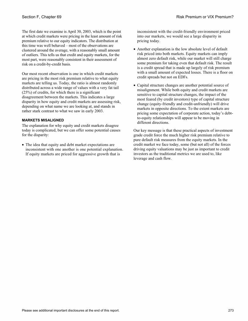
Section F, Chapter 69 Risk Premium or VIX Premium?
Please see additional important disclosures at the end of this report. 273
The first date we examine is April 30, 2003, which is the point at which credit markets were pricing in the least amount of risk premium relative to our equity indicators. The distribution at this time was well behaved – most of the observations are clustered around the average, with a reasonably small amount of outliers. This tells us that credit and equity markets, for the most part, were reasonably consistent in their assessment of risk on a credit-by-credit basis.
Our most recent observation is one in which credit markets are pricing in the most risk premium relative to what equity markets are telling us. Today, the ratio is almost randomly distributed across a wide range of values with a very fat tail (25%) of credits, for which there is a significant disagreement between the markets. This indicates a large disparity in how equity and credit markets are assessing risk, depending on what name we are looking at, and stands in rather stark contrast to what we saw in early 2003.
MARKETS MISALIGNED The explanation for why equity and credit markets disagree today is complicated, but we can offer some potential causes for the disparity:
• The idea that equity and debt market expectations are inconsistent with one another is one potential explanation. If equity markets are priced for aggressive growth that is
inconsistent with the credit-friendly environment priced into our markets, we would see a large disparity in pricing today.
• Another explanation is the low absolute level of default risk priced into both markets. Equity markets can imply almost zero default risk, while our market will still charge some premium for taking even that default risk. The result is a credit spread that is made up largely of risk premium with a small amount of expected losses. There is a floor on credit spreads but not on EDFs.
• Capital structure changes are another potential source of misalignment. While both equity and credit markets are sensitive to capital structure changes, the impact of the most feared (by credit investors) type of capital structure change (equity-friendly and credit-unfriendly) will drive markets in opposite directions. To the extent markets are pricing some expectation of corporate action, today’s debt-to-equity relationships will appear to be moving in different directions.
Our key message is that these practical aspects of investment grade credit force the much higher risk premium relative to pure default risk measures from the equity markets. In the credit market we face today, some (but not all) of the forces driving equity valuations may be just as important to credit investors as the traditional metrics we are used to, like leverage and cash flow.
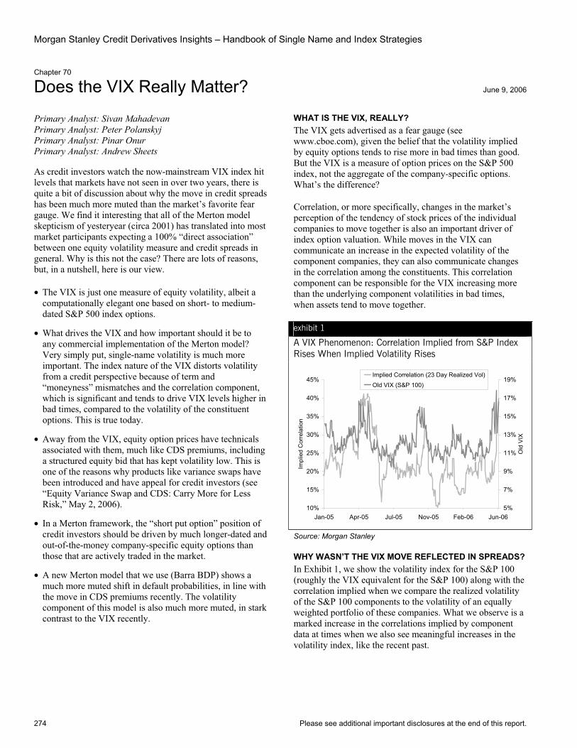
Morgan Stanley Credit Derivatives Insights – Handbook of Single Name and Index Strategies
274 Please see additional important disclosures at the end of this report.
Chapter 70
Does the VIX Really Matter? June 9, 2006
Primary Analyst: Sivan Mahadevan Primary Analyst: Peter Polanskyj Primary Analyst: Pinar Onur Primary Analyst: Andrew Sheets
As credit investors watch the now-mainstream VIX index hit levels that markets have not seen in over two years, there is quite a bit of discussion about why the move in credit spreads has been much more muted than the market’s favorite fear gauge. We find it interesting that all of the Merton model skepticism of yesteryear (circa 2001) has translated into most market participants expecting a 100% “direct association” between one equity volatility measure and credit spreads in general. Why is this not the case? There are lots of reasons, but, in a nutshell, here is our view.
• The VIX is just one measure of equity volatility, albeit a computationally elegant one based on short- to medium-dated S&P 500 index options.
• What drives the VIX and how important should it be to any commercial implementation of the Merton model? Very simply put, single-name volatility is much more important. The index nature of the VIX distorts volatility from a credit perspective because of term and “moneyness” mismatches and the correlation component, which is significant and tends to drive VIX levels higher in bad times, compared to the volatility of the constituent options. This is true today.
• Away from the VIX, equity option prices have technicals associated with them, much like CDS premiums, including a structured equity bid that has kept volatility low. This is one of the reasons why products like variance swaps have been introduced and have appeal for credit investors (see “Equity Variance Swap and CDS: Carry More for Less Risk,” May 2, 2006).
• In a Merton framework, the “short put option” position of credit investors should be driven by much longer-dated and out-of-the-money company-specific equity options than those that are actively traded in the market.
• A new Merton model that we use (Barra BDP) shows a much more muted shift in default probabilities, in line with the move in CDS premiums recently. The volatility component of this model is also much more muted, in stark contrast to the VIX recently.
WHAT IS THE VIX, REALLY? The VIX gets advertised as a fear gauge (see www.cboe.com), given the belief that the volatility implied by equity options tends to rise more in bad times than good. But the VIX is a measure of option prices on the S&P 500 index, not the aggregate of the company-specific options. What’s the difference?
Correlation, or more specifically, changes in the market’s perception of the tendency of stock prices of the individual companies to move together is also an important driver of index option valuation. While moves in the VIX can communicate an increase in the expected volatility of the component companies, they can also communicate changes in the correlation among the constituents. This correlation component can be responsible for the VIX increasing more than the underlying component volatilities in bad times, when assets tend to move together.
exhibit 1
A VIX Phenomenon: Correlation Implied from S&P Index Rises When Implied Volatility Rises
10%
15%
20%
25%
30%
35%
40%
45%
Jan-05 Apr-05 Jul-05 Nov-05 Feb-06 Jun-06
Impl
ied
Cor
rela
tion
5%
7%
9%
11%
13%
15%
17%
19%
Old
VIX
Implied Correlation (23 Day Realized Vol)
Old VIX (S&P 100)
Source: Morgan Stanley
WHY WASN’T THE VIX MOVE REFLECTED IN SPREADS? In Exhibit 1, we show the volatility index for the S&P 100 (roughly the VIX equivalent for the S&P 100) along with the correlation implied when we compare the realized volatility of the S&P 100 components to the volatility of an equally weighted portfolio of these companies. What we observe is a marked increase in the correlations implied by component data at times when we also see meaningful increases in the volatility index, like the recent past.
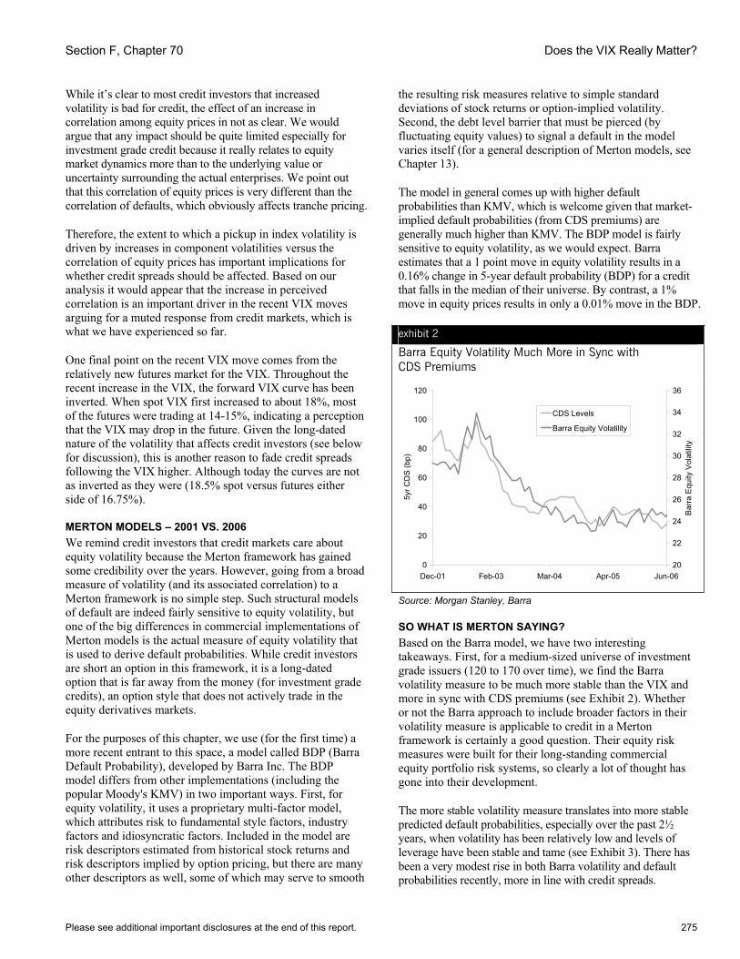
Section F, Chapter 70 Does the VIX Really Matter?
Please see additional important disclosures at the end of this report. 275
While it’s clear to most credit investors that increased volatility is bad for credit, the effect of an increase in correlation among equity prices in not as clear. We would argue that any impact should be quite limited especially for investment grade credit because it really relates to equity market dynamics more than to the underlying value or uncertainty surrounding the actual enterprises. We point out that this correlation of equity prices is very different than the correlation of defaults, which obviously affects tranche pricing.
Therefore, the extent to which a pickup in index volatility is driven by increases in component volatilities versus the correlation of equity prices has important implications for whether credit spreads should be affected. Based on our analysis it would appear that the increase in perceived correlation is an important driver in the recent VIX moves arguing for a muted response from credit markets, which is what we have experienced so far.
One final point on the recent VIX move comes from the relatively new futures market for the VIX. Throughout the recent increase in the VIX, the forward VIX curve has been inverted. When spot VIX first increased to about 18%, most of the futures were trading at 14-15%, indicating a perception that the VIX may drop in the future. Given the long-dated nature of the volatility that affects credit investors (see below for discussion), this is another reason to fade credit spreads following the VIX higher. Although today the curves are not as inverted as they were (18.5% spot versus futures either side of 16.75%).
MERTON MODELS – 2001 VS. 2006 We remind credit investors that credit markets care about equity volatility because the Merton framework has gained some credibility over the years. However, going from a broad measure of volatility (and its associated correlation) to a Merton framework is no simple step. Such structural models of default are indeed fairly sensitive to equity volatility, but one of the big differences in commercial implementations of Merton models is the actual measure of equity volatility that is used to derive default probabilities. While credit investors are short an option in this framework, it is a long-dated option that is far away from the money (for investment grade credits), an option style that does not actively trade in the equity derivatives markets.
For the purposes of this chapter, we use (for the first time) a more recent entrant to this space, a model called BDP (Barra Default Probability), developed by Barra Inc. The BDP model differs from other implementations (including the popular Moody's KMV) in two important ways. First, for equity volatility, it uses a proprietary multi-factor model, which attributes risk to fundamental style factors, industry factors and idiosyncratic factors. Included in the model are risk descriptors estimated from historical stock returns and risk descriptors implied by option pricing, but there are many other descriptors as well, some of which may serve to smooth
the resulting risk measures relative to simple standard deviations of stock returns or option-implied volatility. Second, the debt level barrier that must be pierced (by fluctuating equity values) to signal a default in the model varies itself (for a general description of Merton models, see Chapter 13).
The model in general comes up with higher default probabilities than KMV, which is welcome given that market-implied default probabilities (from CDS premiums) are generally much higher than KMV. The BDP model is fairly sensitive to equity volatility, as we would expect. Barra estimates that a 1 point move in equity volatility results in a 0.16% change in 5-year default probability (BDP) for a credit that falls in the median of their universe. By contrast, a 1% move in equity prices results in only a 0.01% move in the BDP.
exhibit 2
Barra Equity Volatility Much More in Sync with CDS Premiums
0
20
40
60
80
100
120
Dec-01 Feb-03 Mar-04 Apr-05 Jun-06
5yr C
DS
(bp)
20
22
24
26
28
30
32
34
36
Bar
ra E
quity
Vol
atilit
y
CDS Levels
Barra Equity Volatility
Source: Morgan Stanley, Barra
SO WHAT IS MERTON SAYING? Based on the Barra model, we have two interesting takeaways. First, for a medium-sized universe of investment grade issuers (120 to 170 over time), we find the Barra volatility measure to be much more stable than the VIX and more in sync with CDS premiums (see Exhibit 2). Whether or not the Barra approach to include broader factors in their volatility measure is applicable to credit in a Merton framework is certainly a good question. Their equity risk measures were built for their long-standing commercial equity portfolio risk systems, so clearly a lot of thought has gone into their development.
The more stable volatility measure translates into more stable predicted default probabilities, especially over the past 2½ years, when volatility has been relatively low and levels of leverage have been stable and tame (see Exhibit 3). There has been a very modest rise in both Barra volatility and default probabilities recently, more in line with credit spreads.
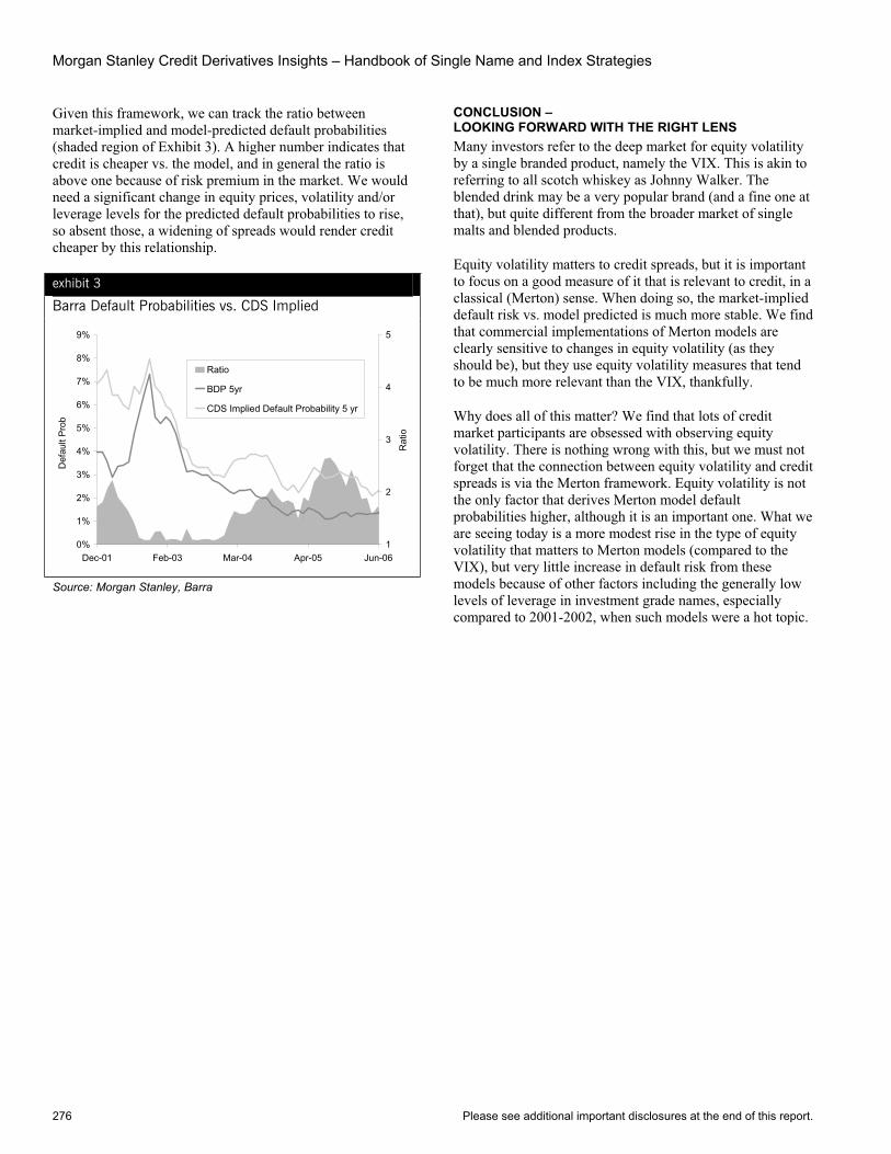
Morgan Stanley Credit Derivatives Insights – Handbook of Single Name and Index Strategies
276 Please see additional important disclosures at the end of this report.
Given this framework, we can track the ratio between market-implied and model-predicted default probabilities (shaded region of Exhibit 3). A higher number indicates that credit is cheaper vs. the model, and in general the ratio is above one because of risk premium in the market. We would need a significant change in equity prices, volatility and/or leverage levels for the predicted default probabilities to rise, so absent those, a widening of spreads would render credit cheaper by this relationship.
exhibit 3
Barra Default Probabilities vs. CDS Implied
0%
1%
2%
3%
4%
5%
6%
7%
8%
9%
Dec-01 Feb-03 Mar-04 Apr-05 Jun-06
Def
ault
Prob
1
2
3
4
5
Rat
io
Ratio
BDP 5yr
CDS Implied Default Probability 5 yr
Source: Morgan Stanley, Barra
CONCLUSION –LOOKING FORWARD WITH THE RIGHT LENS Many investors refer to the deep market for equity volatility by a single branded product, namely the VIX. This is akin to referring to all scotch whiskey as Johnny Walker. The blended drink may be a very popular brand (and a fine one at that), but quite different from the broader market of single malts and blended products.
Equity volatility matters to credit spreads, but it is important to focus on a good measure of it that is relevant to credit, in a classical (Merton) sense. When doing so, the market-implied default risk vs. model predicted is much more stable. We find that commercial implementations of Merton models are clearly sensitive to changes in equity volatility (as they should be), but they use equity volatility measures that tend to be much more relevant than the VIX, thankfully.
Why does all of this matter? We find that lots of credit market participants are obsessed with observing equity volatility. There is nothing wrong with this, but we must not forget that the connection between equity volatility and credit spreads is via the Merton framework. Equity volatility is not the only factor that derives Merton model default probabilities higher, although it is an important one. What we are seeing today is a more modest rise in the type of equity volatility that matters to Merton models (compared to the VIX), but very little increase in default risk from these models because of other factors including the generally low levels of leverage in investment grade names, especially compared to 2001-2002, when such models were a hot topic.
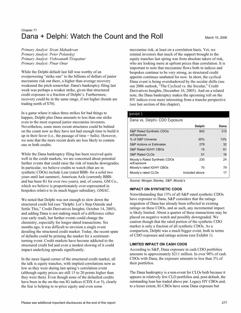
Please see additional important disclosures at the end of this report. 277
Chapter 71
Dana + Delphi: Watch the Count and the Roll March 10, 2006
Primary Analyst: Sivan Mahadevan Primary Analyst: Peter Polanskyj Primary Analyst: Vishwanath Tirupattur Primary Analyst: Pinar Onur
While the Delphi default last fall was worthy of an overpowering “strike one” to the billions of dollars of junior mezzanine risk out there, a higher than average recovery weakened the pitch somewhat. Dana's bankruptcy filing last week was perhaps a weaker strike, given that structured credit exposure is a fraction of Delphi’s. Furthermore, recovery could be in the same range, if not higher (bonds are trading north of $70).
In a game where it takes three strikes for bad things to happen, Delphi plus Dana amounts to less than one strike even to the most exposed junior mezzanine investors. Nevertheless, some more recent structures could be behind on the count now as they have not had enough time to build it up in their favor (i.e., the passage of time = balls). However, we note that the more recent deals are less likely to contain one or both credits.
While the Dana bankruptcy filing has been received quite well in the credit markets, we are concerned about potential further events that could raise the risk of tranche downgrades. In particular, we believe credits to watch (that are in synthetic CDOs) include Lear (rated BBB- for a solid two years until last summer), American Axle (currently BBB- and has been IG for over two years), and, of course, GM Co., which we believe is proportionately over-represented in bespokes relative to its much bigger subsidiary, GMAC.
We noted that Delphi was not enough to slow down the structured credit bid (see “Delphi: Let’s Step Outside and Settle This,” Credit Derivatives Insights, October 14, 2005), and adding Dana is not making much of a difference either (our early read), but further events could change the chemistry, especially for longer-dated transactions. Six months ago, it was difficult to envision a single event derailing the structured credit market. Today, the recent spate of defaults could be priming the market for a sentiment-turning event. Credit markets have become addicted to the structured credit bid and even a modest slowing of it could impact underlying spreads significantly.
In the more liquid corner of the structured credit market, all the talk is equity tranches, with implied correlations now as low as they were during last spring’s correlation event (although equity prices are still 15 to 20 points higher than they were then). Even though none of the defaulted credits have been in the on-the-run IG indices (CDX 4 or 5), clearly the fear is helping to re-price equity and even some
mezzanine risk, at least on a correlation basis. Yet, we remind investors that much of the support brought to the equity tranches last spring was from absolute takers of risk, who are looking more at upfront prices than correlation. It is important to note that mezzanine flows both in indices and bespokes continue to be very strong, as structured credit appetite continues unabated for now. In short, the cyclical Dana event is being overshadowed by the secular shifts (see our 2006 outlook, “The Cyclical vs. the Secular,” Credit Derivatives Insights, December 16, 2005). And on a related note, the Dana bankruptcy makes the upcoming roll on the HY indices even more interesting from a tranche perspective (see last section of this chapter).
exhibit 1
Dana vs. Delphi: CDO Exposure Delphi Dana
S&P Rated Synthetic CDOs w/Exposure
842 315
% of S&P Universe 35% 13%S&P Actions or Estimates 278 32S&P Rated IG/HY CBOs 15 61S&P Rated CLOs 51 16Moody’s Rated Synthetic CDOs w/Exposure
230 24
Moody’s rated IG/HY CBOs 70 79Moody’s rated CLOs Included above 17
Source: Morgan Stanley, S&P, Moody’s
IMPACT ON SYNTHETIC CDOS Notwithstanding that 13% of all S&P rated synthetic CDOs have exposure to Dana, S&P considers that the ratings migration of Dana has already been reflected in existing ratings on these CDOs, and as such, any incremental impact is likely limited. About a quarter of these transactions may be placed on negative watch and possibly downgraded. We caution though that the rated portion of the synthetic CDO market is only a fraction of all synthetic CDOs. As a comparison, Delphi was a much bigger event, both in terms of CDO exposure and ratings actions (see Exhibit 1).
LIMITED IMPACT ON CASH CDOS According to S&P, Dana exposure in cash CDO portfolios amounts to approximately $211 million. In over 90% of cash CDOs with Dana, the exposure amounts to less than 3% of their portfolios.
The Dana bankruptcy is a non-event for CLOs both because it appears in relatively few CLO portfolios and, post-default, the outstanding loan has traded above par. Legacy HY CBOs and, to a lesser extent, IG CBOs have some Dana exposure but
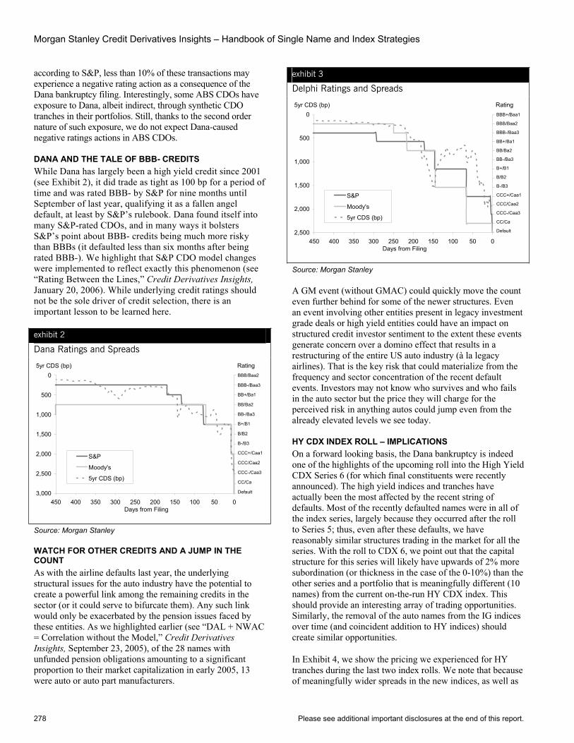
Morgan Stanley Credit Derivatives Insights – Handbook of Single Name and Index Strategies
278 Please see additional important disclosures at the end of this report.
according to S&P, less than 10% of these transactions may experience a negative rating action as a consequence of the Dana bankruptcy filing. Interestingly, some ABS CDOs have exposure to Dana, albeit indirect, through synthetic CDO tranches in their portfolios. Still, thanks to the second order nature of such exposure, we do not expect Dana-caused negative ratings actions in ABS CDOs.
DANA AND THE TALE OF BBB- CREDITS While Dana has largely been a high yield credit since 2001 (see Exhibit 2), it did trade as tight as 100 bp for a period of time and was rated BBB- by S&P for nine months until September of last year, qualifying it as a fallen angel default, at least by S&P’s rulebook. Dana found itself into many S&P-rated CDOs, and in many ways it bolsters S&P’s point about BBB- credits being much more risky than BBBs (it defaulted less than six months after being rated BBB-). We highlight that S&P CDO model changes were implemented to reflect exactly this phenomenon (see “Rating Between the Lines,” Credit Derivatives Insights,January 20, 2006). While underlying credit ratings should not be the sole driver of credit selection, there is an important lesson to be learned here.
exhibit 2
Dana Ratings and Spreads
5yr CDS (bp)
0123456789101112
050100150200250300350400450Days from Filing
Rating0
500
1,000
1,500
2,000
2,500
3,000
S&P
Moody's
5yr CDS (bp)
CCC+/Caa1
CCC/Caa2
CCC-/Caa3
B-/B3
B/B2
B+/B1
BB-/Ba3
BB/Ba2
BB+/Ba1
BBB-/Baa3
BBB/Baa2
CC/Ca
Default
Source: Morgan Stanley
WATCH FOR OTHER CREDITS AND A JUMP IN THE COUNTAs with the airline defaults last year, the underlying structural issues for the auto industry have the potential to create a powerful link among the remaining credits in the sector (or it could serve to bifurcate them). Any such link would only be exacerbated by the pension issues faced by these entities. As we highlighted earlier (see “DAL + NWAC = Correlation without the Model,” Credit Derivatives Insights, September 23, 2005), of the 28 names with unfunded pension obligations amounting to a significant proportion to their market capitalization in early 2005, 13 were auto or auto part manufacturers.
exhibit 3
Delphi Ratings and Spreads
5yr CDS (bp)
012345678910111213
050100150200250300350400450Days from Filing
Rating0
500
1,000
1,500
2,000
2,500
S&P
Moody's
5yr CDS (bp)
CCC+/Caa1
CCC/Caa2
CCC-/Caa3
B-/B3
B/B2
B+/B1
BB-/Ba3
BB/Ba2
BB+/Ba1
BBB-/Baa3
BBB/Baa2
BBB+/Baa1
CC/Ca
Default
Source: Morgan Stanley
A GM event (without GMAC) could quickly move the count even further behind for some of the newer structures. Even an event involving other entities present in legacy investment grade deals or high yield entities could have an impact on structured credit investor sentiment to the extent these events generate concern over a domino effect that results in a restructuring of the entire US auto industry (à la legacy airlines). That is the key risk that could materialize from the frequency and sector concentration of the recent default events. Investors may not know who survives and who fails in the auto sector but the price they will charge for the perceived risk in anything autos could jump even from the already elevated levels we see today.
HY CDX INDEX ROLL – IMPLICATIONS On a forward looking basis, the Dana bankruptcy is indeed one of the highlights of the upcoming roll into the High Yield CDX Series 6 (for which final constituents were recently announced). The high yield indices and tranches have actually been the most affected by the recent string of defaults. Most of the recently defaulted names were in all of the index series, largely because they occurred after the roll to Series 5; thus, even after these defaults, we have reasonably similar structures trading in the market for all the series. With the roll to CDX 6, we point out that the capital structure for this series will likely have upwards of 2% more subordination (or thickness in the case of the 0-10%) than the other series and a portfolio that is meaningfully different (10 names) from the current on-the-run HY CDX index. This should provide an interesting array of trading opportunities. Similarly, the removal of the auto names from the IG indices over time (and coincident addition to HY indices) should create similar opportunities.
In Exhibit 4, we show the pricing we experienced for HY tranches during the last two index rolls. We note that because of meaningfully wider spreads in the new indices, as well as
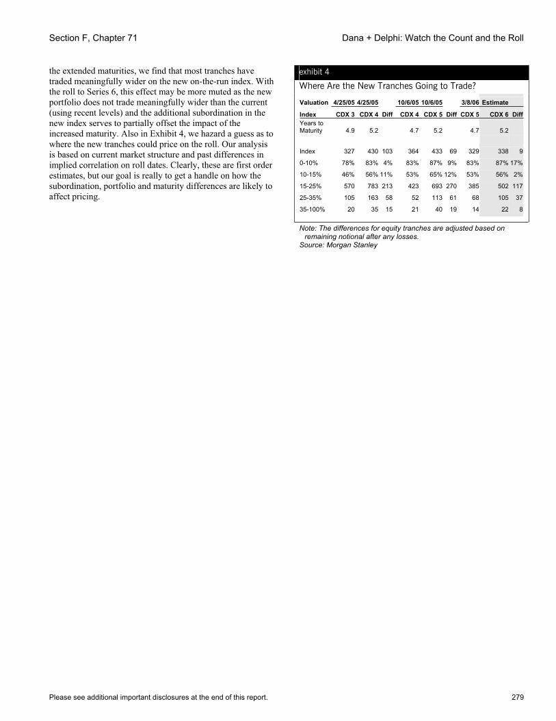
Section F, Chapter 71 Dana + Delphi: Watch the Count and the Roll
Please see additional important disclosures at the end of this report. 279
the extended maturities, we find that most tranches have traded meaningfully wider on the new on-the-run index. With the roll to Series 6, this effect may be more muted as the new portfolio does not trade meaningfully wider than the current (using recent levels) and the additional subordination in the new index serves to partially offset the impact of the increased maturity. Also in Exhibit 4, we hazard a guess as to where the new tranches could price on the roll. Our analysis is based on current market structure and past differences in implied correlation on roll dates. Clearly, these are first order estimates, but our goal is really to get a handle on how the subordination, portfolio and maturity differences are likely to affect pricing.
exhibit 4
Where Are the New Tranches Going to Trade?
Valuation 4/25/05 4/25/05 10/6/05 10/6/05 3/8/06 Estimate
Index CDX 3 CDX 4 Diff CDX 4 CDX 5 Diff CDX 5 CDX 6 DiffYears to Maturity 4.9 5.2 4.7 5.2 4.7 5.2
Index 327 430 103 364 433 69 329 338 9
0-10% 78% 83% 4% 83% 87% 9% 83% 87% 17%
10-15% 46% 56% 11% 53% 65% 12% 53% 56% 2%
15-25% 570 783 213 423 693 270 385 502 117
25-35% 105 163 58 52 113 61 68 105 37
35-100% 20 35 15 21 40 19 14 22 8
Note: The differences for equity tranches are adjusted based on remaining notional after any losses.
Source: Morgan Stanley
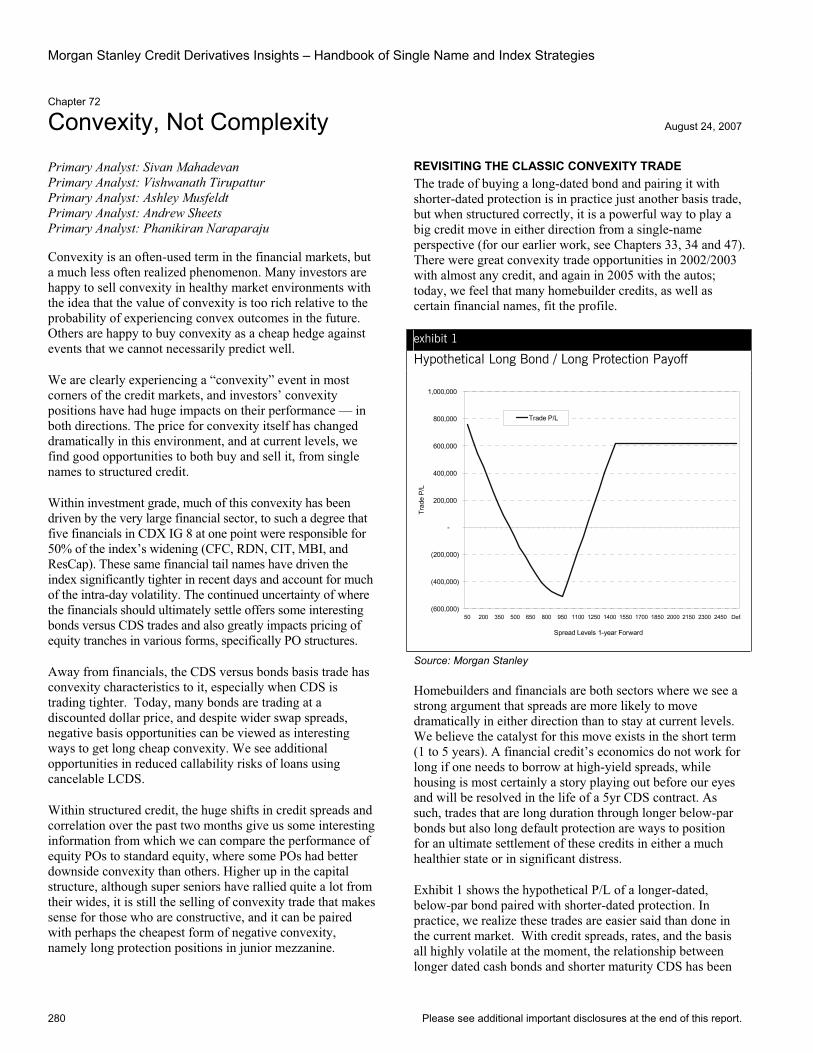
Morgan Stanley Credit Derivatives Insights – Handbook of Single Name and Index Strategies
280 Please see additional important disclosures at the end of this report.
Chapter 72
Convexity, Not Complexity August 24, 2007
Primary Analyst: Sivan Mahadevan Primary Analyst: Vishwanath Tirupattur Primary Analyst: Ashley Musfeldt Primary Analyst: Andrew Sheets Primary Analyst: Phanikiran Naraparaju
Convexity is an often-used term in the financial markets, but a much less often realized phenomenon. Many investors are happy to sell convexity in healthy market environments with the idea that the value of convexity is too rich relative to the probability of experiencing convex outcomes in the future. Others are happy to buy convexity as a cheap hedge against events that we cannot necessarily predict well.
We are clearly experiencing a “convexity” event in most corners of the credit markets, and investors’ convexity positions have had huge impacts on their performance — in both directions. The price for convexity itself has changed dramatically in this environment, and at current levels, we find good opportunities to both buy and sell it, from single names to structured credit.
Within investment grade, much of this convexity has been driven by the very large financial sector, to such a degree that five financials in CDX IG 8 at one point were responsible for 50% of the index’s widening (CFC, RDN, CIT, MBI, and ResCap). These same financial tail names have driven the index significantly tighter in recent days and account for much of the intra-day volatility. The continued uncertainty of where the financials should ultimately settle offers some interesting bonds versus CDS trades and also greatly impacts pricing of equity tranches in various forms, specifically PO structures.
Away from financials, the CDS versus bonds basis trade has convexity characteristics to it, especially when CDS is trading tighter. Today, many bonds are trading at a discounted dollar price, and despite wider swap spreads, negative basis opportunities can be viewed as interesting ways to get long cheap convexity. We see additional opportunities in reduced callability risks of loans using cancelable LCDS.
Within structured credit, the huge shifts in credit spreads and correlation over the past two months give us some interesting information from which we can compare the performance of equity POs to standard equity, where some POs had better downside convexity than others. Higher up in the capital structure, although super seniors have rallied quite a lot from their wides, it is still the selling of convexity trade that makes sense for those who are constructive, and it can be paired with perhaps the cheapest form of negative convexity, namely long protection positions in junior mezzanine.
REVISITING THE CLASSIC CONVEXITY TRADE The trade of buying a long-dated bond and pairing it with shorter-dated protection is in practice just another basis trade, but when structured correctly, it is a powerful way to play a big credit move in either direction from a single-name perspective (for our earlier work, see Chapters 33, 34 and 47). There were great convexity trade opportunities in 2002/2003 with almost any credit, and again in 2005 with the autos; today, we feel that many homebuilder credits, as well as certain financial names, fit the profile.
exhibit 1
Hypothetical Long Bond / Long Protection Payoff
(600,000)
(400,000)
(200,000)
-
200,000
400,000
600,000
800,000
1,000,000
50 200 350 500 650 800 950 1100 1250 1400 1550 1700 1850 2000 2150 2300 2450 Def.
Spread Levels 1-year Forward
Trad
e P
/LTrade P/L
Source: Morgan Stanley
Homebuilders and financials are both sectors where we see a strong argument that spreads are more likely to move dramatically in either direction than to stay at current levels. We believe the catalyst for this move exists in the short term (1 to 5 years). A financial credit’s economics do not work for long if one needs to borrow at high-yield spreads, while housing is most certainly a story playing out before our eyes and will be resolved in the life of a 5yr CDS contract. As such, trades that are long duration through longer below-par bonds but also long default protection are ways to position for an ultimate settlement of these credits in either a much healthier state or in significant distress.
Exhibit 1 shows the hypothetical P/L of a longer-dated, below-par bond paired with shorter-dated protection. In practice, we realize these trades are easier said than done in the current market. With credit spreads, rates, and the basis all highly volatile at the moment, the relationship between longer dated cash bonds and shorter maturity CDS has been
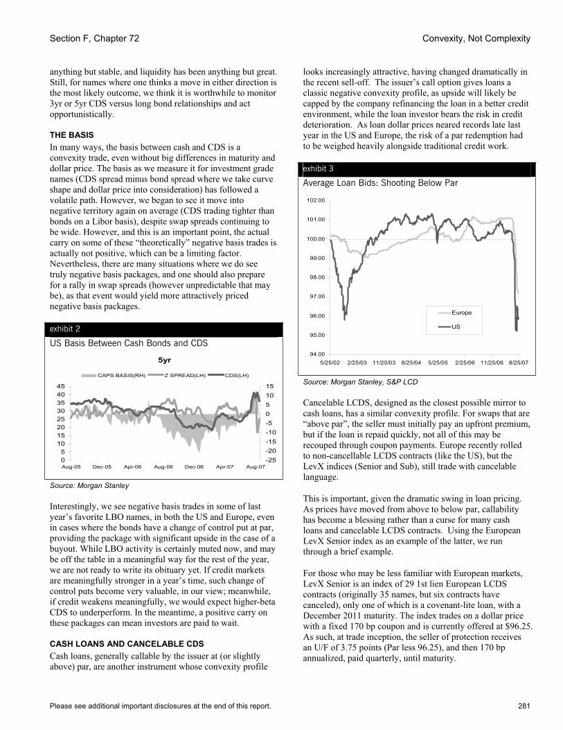
Section F, Chapter 72 Convexity, Not Complexity
Please see additional important disclosures at the end of this report. 281
anything but stable, and liquidity has been anything but great. Still, for names where one thinks a move in either direction is the most likely outcome, we think it is worthwhile to monitor 3yr or 5yr CDS versus long bond relationships and act opportunistically.
THE BASIS In many ways, the basis between cash and CDS is a convexity trade, even without big differences in maturity and dollar price. The basis as we measure it for investment grade names (CDS spread minus bond spread where we take curve shape and dollar price into consideration) has followed a volatile path. However, we began to see it move into negative territory again on average (CDS trading tighter than bonds on a Libor basis), despite swap spreads continuing to be wide. However, and this is an important point, the actual carry on some of these “theoretically” negative basis trades is actually not positive, which can be a limiting factor. Nevertheless, there are many situations where we do see truly negative basis packages, and one should also prepare for a rally in swap spreads (however unpredictable that may be), as that event would yield more attractively priced negative basis packages.
exhibit 2
US Basis Between Cash Bonds and CDS
5yr
05
1015202530354045
Aug-05 Dec-05 Apr-06 Aug-06 Dec-06 Apr-07 Aug-07-25-20-15-10-5051015
CAPS BASIS(RH) Z SPREAD(LH) CDS(LH)
Source: Morgan Stanley
Interestingly, we see negative basis trades in some of last year’s favorite LBO names, in both the US and Europe, even in cases where the bonds have a change of control put at par, providing the package with significant upside in the case of a buyout. While LBO activity is certainly muted now, and may be off the table in a meaningful way for the rest of the year, we are not ready to write its obituary yet. If credit markets are meaningfully stronger in a year’s time, such change of control puts become very valuable, in our view; meanwhile, if credit weakens meaningfully, we would expect higher-beta CDS to underperform. In the meantime, a positive carry on these packages can mean investors are paid to wait.
CASH LOANS AND CANCELABLE CDS Cash loans, generally callable by the issuer at (or slightly above) par, are another instrument whose convexity profile
looks increasingly attractive, having changed dramatically in the recent sell-off. The issuer’s call option gives loans a classic negative convexity profile, as upside will likely be capped by the company refinancing the loan in a better credit environment, while the loan investor bears the risk in credit deterioration. As loan dollar prices neared records late last year in the US and Europe, the risk of a par redemption had to be weighed heavily alongside traditional credit work.
exhibit 3
Average Loan Bids: Shooting Below Par
94.00
95.00
96.00
97.00
98.00
99.00
100.00
101.00
102.00
5/25/02 2/25/03 11/25/03 8/25/04 5/25/05 2/25/06 11/25/06 8/25/07
Europe
US
Source: Morgan Stanley, S&P LCD
Cancelable LCDS, designed as the closest possible mirror to cash loans, has a similar convexity profile. For swaps that are “above par”, the seller must initially pay an upfront premium, but if the loan is repaid quickly, not all of this may be recouped through coupon payments. Europe recently rolled to non-cancellable LCDS contracts (like the US), but the LevX indices (Senior and Sub), still trade with cancelable language.
This is important, given the dramatic swing in loan pricing. As prices have moved from above to below par, callability has become a blessing rather than a curse for many cash loans and cancelable LCDS contracts. Using the European LevX Senior index as an example of the latter, we run through a brief example.
For those who may be less familiar with European markets, LevX Senior is an index of 29 1st lien European LCDS contracts (originally 35 names, but six contracts have canceled), only one of which is a covenant-lite loan, with a December 2011 maturity. The index trades on a dollar price with a fixed 170 bp coupon and is currently offered at $96.25. As such, at trade inception, the seller of protection receives an U/F of 3.75 points (Par less 96.25), and then 170 bp annualized, paid quarterly, until maturity.
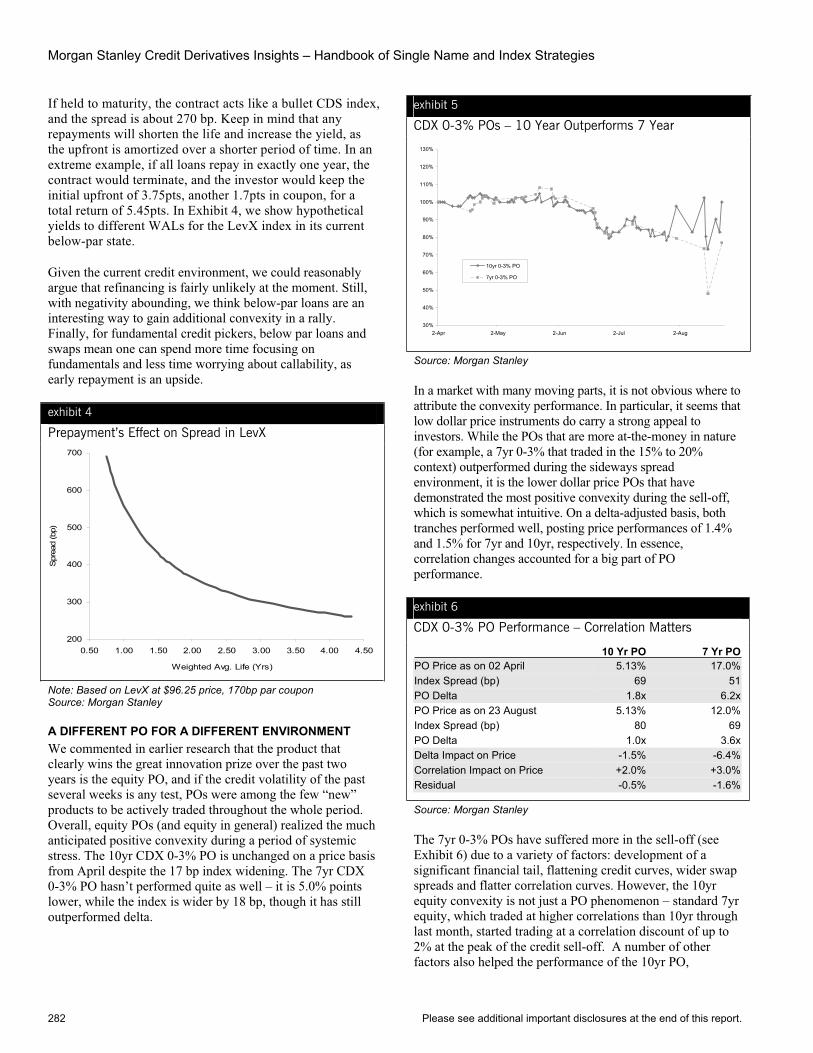
Morgan Stanley Credit Derivatives Insights – Handbook of Single Name and Index Strategies
282 Please see additional important disclosures at the end of this report.
If held to maturity, the contract acts like a bullet CDS index, and the spread is about 270 bp. Keep in mind that any repayments will shorten the life and increase the yield, as the upfront is amortized over a shorter period of time. In an extreme example, if all loans repay in exactly one year, the contract would terminate, and the investor would keep the initial upfront of 3.75pts, another 1.7pts in coupon, for a total return of 5.45pts. In Exhibit 4, we show hypothetical yields to different WALs for the LevX index in its current below-par state.
Given the current credit environment, we could reasonably argue that refinancing is fairly unlikely at the moment. Still, with negativity abounding, we think below-par loans are an interesting way to gain additional convexity in a rally. Finally, for fundamental credit pickers, below par loans and swaps mean one can spend more time focusing on fundamentals and less time worrying about callability, as early repayment is an upside.
exhibit 4
Prepayment’s Effect on Spread in LevX
200
300
400
500
600
700
0.50 1.00 1.50 2.00 2.50 3.00 3.50 4.00 4.50
Weighted Avg. Life (Yrs)
Spr
ead
(bp)
Note: Based on LevX at $96.25 price, 170bp par coupon Source: Morgan Stanley
A DIFFERENT PO FOR A DIFFERENT ENVIRONMENT We commented in earlier research that the product that clearly wins the great innovation prize over the past two years is the equity PO, and if the credit volatility of the past several weeks is any test, POs were among the few “new” products to be actively traded throughout the whole period. Overall, equity POs (and equity in general) realized the much anticipated positive convexity during a period of systemic stress. The 10yr CDX 0-3% PO is unchanged on a price basis from April despite the 17 bp index widening. The 7yr CDX 0-3% PO hasn’t performed quite as well – it is 5.0% points lower, while the index is wider by 18 bp, though it has still outperformed delta.
exhibit 5
CDX 0-3% POs – 10 Year Outperforms 7 Year
30%
40%
50%
60%
70%
80%
90%
100%
110%
120%
130%
2-Apr 2-May 2-Jun 2-Jul 2-Aug
10yr 0-3% PO
7yr 0-3% PO
Source: Morgan Stanley
In a market with many moving parts, it is not obvious where to attribute the convexity performance. In particular, it seems that low dollar price instruments do carry a strong appeal to investors. While the POs that are more at-the-money in nature (for example, a 7yr 0-3% that traded in the 15% to 20% context) outperformed during the sideways spread environment, it is the lower dollar price POs that have demonstrated the most positive convexity during the sell-off, which is somewhat intuitive. On a delta-adjusted basis, both tranches performed well, posting price performances of 1.4% and 1.5% for 7yr and 10yr, respectively. In essence, correlation changes accounted for a big part of PO performance.
exhibit 6
CDX 0-3% PO Performance – Correlation Matters
10 Yr PO 7 Yr PO PO Price as on 02 April 5.13% 17.0%Index Spread (bp) 69 51PO Delta 1.8x 6.2xPO Price as on 23 August 5.13% 12.0%Index Spread (bp) 80 69PO Delta 1.0x 3.6xDelta Impact on Price -1.5% -6.4%Correlation Impact on Price +2.0% +3.0%Residual -0.5% -1.6%
Source: Morgan Stanley
The 7yr 0-3% POs have suffered more in the sell-off (see Exhibit 6) due to a variety of factors: development of a significant financial tail, flattening credit curves, wider swap spreads and flatter correlation curves. However, the 10yr equity convexity is not just a PO phenomenon – standard 7yr equity, which traded at higher correlations than 10yr through last month, started trading at a correlation discount of up to 2% at the peak of the credit sell-off. A number of other factors also helped the performance of the 10yr PO,

Section F, Chapter 72 Convexity, Not Complexity
Please see additional important disclosures at the end of this report. 283
including the flattening of credit curves driven both by the widening of the financials and the collapse of the LBO premium in curves.
From a rates perspective, despite the volatility, USD Libor rates are only 20 bp tighter from the mid-July peak. The dollar price impact of rate moves is about 0.3-0.7 points for different types of POs, i.e., 6-8% of the dollar prices – certainly non-trivial but still only a small component of the overall performance.
Going forward, different spread environments call for different PO choices. The deep-OTM equity POs like 10yr 0-
3% pack more convexity, which is valuable in the current volatile spread environment. But if milder climates return, the 7yr 0-3% type POs are much better positioned to monetize the upside.
CONCLUSION – CONVEXITY IS NOT COMPLEX We continue to believe that convexity can be a big driver of performance, as it has been in the recent past. With the price of convexity changing, we find opportunities in long bond versus short protection, negative basis trades in general, below par loans and cancelable LCDS. And finally, certain equity PO strategies appear to be very attractive plays on credit convexity at current market prices.
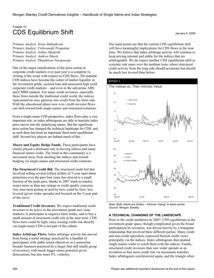
Morgan Stanley Credit Derivatives Insights – Handbook of Single Name and Index Strategies
284 Please see additional important disclosures at the end of this report.
Chapter 73
CDS Equilibrium Shift January 4, 2008
Primary Analyst: Sivan Mahadevan Primary Analyst: Vishwanath Tirupattur Primary Analyst: Ashley Musfeldt Primary Analyst: Andrew Sheets Primary Analyst: Phanikiran Naraparaju
One of the major ramifications of the price action in corporate credit markets over past year is a complete re-writing of the script with respect to CDS flows. The popular CDS indices have become the center of market liquidity in the investment grade, secured loan and unsecured high yield corporate credit markets – and even in the sub-prime ABS and CMBS markets. For many credit investors, especially those from outside the traditional credit world, the indices represented an easy gateway into credit from the short side. With the educational phase now over, credit investor flows can shift toward both single-names and structured solutions.
From a single-name CDS perspective, index flows play a very important role, as index arbitrageurs are able to translate index price moves into the underlying names. But the significant price action has changed the technical landscape for CDS, and as such there has been an important short-term equilibrium shift. Several key players are behind much of this.
Macro and Equity Hedge Funds. These participants have clearly played a dominant role in moving indices and many financial names wider. The trend in this community is a movement away from shorting the indices and toward hedging via single names and structured credit solutions.
The Structured Credit Bid. The structured credit bid that involved selling several trillion dollars of 5-year equivalent protection over the past four years has slowed to a small fraction of the peak pace, thanks to 2007 mark-to-market issues more so than any ratings or credit quality concerns. Any near-term pickup in activity here could be slow, less levered (given wider spreads) and focused on the 5-year part of the curve.
Traditional Credit Investors. We expect traditional credit investors to be active in the investment grade new issue markets, to participate in negative basis trades, and to buy a small amount of structured credit risk in the near term. CDS flows here could be light, since owning credit risk directly via single-name CDS is not part of the culture.
Index Arbitrage Flows. Index arbitrage activity has moved from being a niche strategy practiced by a handful of participants with stable return objectives to a somewhat broader business practiced by a larger (but still small) group of investors, with much bigger return potential given dislocations, but also more P/L volatility.
Our main points are that the current CDS equilibrium shift will have meaningful implications for CDS flows in the near term. We believe that index arbitrage activity will continue to keep pricing rational and stable for the indices that are arbitrageable. We do expect another CDS equilibrium shift as systemic risk eases over the medium term, where structured credit activity from the long side should accelerate but should be much less levered than before.
exhibit 1
The Indices vs. Their Intrinsic Value
-10
-5
0
5
10
15
Sep-06 Dec-06 Mar-07 Jun-07 Sep-07 Dec-07
CDX IG 5yr
iTraxx 5yr
-40
-20
0
20
40
60
80
100
Mar-07 Jun-07 Sep-07 Dec-07
CDX HY
LCDX
iTraxx XOVER
Note: Both charts are [Index – Intrinsic Value], in basis points. Source: Morgan Stanley
A TECHNICAL CHANGING OF THE LANDSCAPE Prior to the credit meltdown in 2H07, CDS equilibrium in the investment grade space, though complicated given the broad participation by investors, was driven heavily by a triangular relationship that involved three different parties. Many credit and non-credit specialists expressed bearish credit views principally via the indices. Index arbitrageurs then pushed single-names wider to synch them with the indices. Finally, structured credit investors then saw wider spreads as an invitation to buy more credit risk via mezzanine tranches. Index arbitrageurs synchronized again, and the triangle often
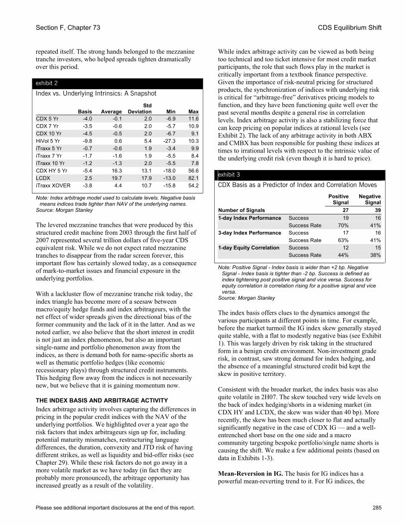
Section F, Chapter 73 CDS Equilibrium Shift
Please see additional important disclosures at the end of this report. 285
repeated itself. The strong hands belonged to the mezzanine tranche investors, who helped spreads tighten dramatically over this period.
exhibit 2
Index vs. Underlying Intrinsics: A Snapshot
Basis AverageStd
Deviation Min MaxCDX 5 Yr -4.0 -0.1 2.0 -6.9 11.6CDX 7 Yr -3.5 -0.6 2.0 -5.7 10.9CDX 10 Yr -4.5 -0.5 2.0 -6.7 9.1HiVol 5 Yr -9.8 0.6 5.4 -27.3 10.3iTraxx 5 Yr -0.7 -0.6 1.9 -3.4 9.9iTraxx 7 Yr -1.7 -1.6 1.9 -5.5 8.4iTraxx 10 Yr -1.2 -1.3 2.0 -5.5 7.8CDX HY 5 Yr -5.4 16.3 13.1 -18.0 56.6LCDX 2.5 19.7 17.9 -13.0 82.1iTraxx XOVER -3.8 4.4 10.7 -15.8 54.2
Note: Index arbitrage model used to calculate levels. Negative basis means indices trade tighter than NAV of the underlying names.
Source: Morgan Stanley
The levered mezzanine tranches that were produced by this structured credit machine from 2003 through the first half of 2007 represented several trillion dollars of five-year CDS equivalent risk. While we do not expect rated mezzanine tranches to disappear from the radar screen forever, this important flow has certainly slowed today, as a consequence of mark-to-market issues and financial exposure in the underlying portfolios.
With a lackluster flow of mezzanine tranche risk today, the index triangle has become more of a seesaw between macro/equity hedge funds and index arbitrageurs, with the net effect of wider spreads given the directional bias of the former community and the lack of it in the latter. And as we noted earlier, we also believe that the short interest in credit is not just an index phenomenon, but also an important single-name and portfolio phenomenon away from the indices, as there is demand both for name-specific shorts as well as thematic portfolio hedges (like economic recessionary plays) through structured credit instruments. This hedging flow away from the indices is not necessarily new, but we believe that it is gaining momentum now.
THE INDEX BASIS AND ARBITRAGE ACTIVITY Index arbitrage activity involves capturing the differences in pricing in the popular credit indices with the NAV of the underlying portfolios. We highlighted over a year ago the risk factors that index arbitrageurs sign up for, including potential maturity mismatches, restructuring language differences, the duration, convexity and JTD risk of having different strikes, as well as liquidity and bid-offer risks (see Chapter 29). While these risk factors do not go away in a more volatile market as we have today (in fact they are probably more pronounced), the arbitrage opportunity has increased greatly as a result of the volatility.
While index arbitrage activity can be viewed as both being too technical and too ticket intensive for most credit market participants, the role that such flows play in the market is critically important from a textbook finance perspective. Given the importance of risk-neutral pricing for structured products, the synchronization of indices with underlying risk is critical for “arbitrage-free” derivatives pricing models to function, and they have been functioning quite well over the past several months despite a general rise in correlation levels. Index arbitrage activity is also a stabilizing force that can keep pricing on popular indices at rational levels (see Exhibit 2). The lack of any arbitrage activity in both ABX and CMBX has been responsible for pushing these indices at times to irrational levels with respect to the intrinsic value of the underlying credit risk (even though it is hard to price).
exhibit 3
CDX Basis as a Predictor of Index and Correlation Moves
Positive
SignalNegative
SignalNumber of Signals 27 391-day Index Performance Success 19 16
Success Rate 70% 41%3-day Index Performance Success 17 16
Success Rate 63% 41%1-day Equity Correlation Success 12 15
Success Rate 44% 38%
Note: Positive Signal - Index basis is wider than +2 bp. Negative Signal - Index basis is tighter than -2 bp. Success is defined as index tightening post positive signal and vice versa. Success for equity correlation is correlation rising for a positive signal and vice versa.
Source: Morgan Stanley
The index basis offers clues to the dynamics amongst the various participants at different points in time. For example, before the market turmoil the IG index skew generally stayed quite stable, with a flat to modestly negative bias (see Exhibit 1). This was largely driven by risk taking in the structured form in a benign credit environment. Non-investment grade risk, in contrast, saw strong demand for index hedging, and the absence of a meaningful structured credit bid kept the skew in positive territory.
Consistent with the broader market, the index basis was also quite volatile in 2H07. The skew touched very wide levels on the back of index hedging/shorts in a widening market (in CDX HY and LCDX, the skew was wider than 40 bp). More recently, the skew has been much closer to flat and actually significantly negative in the case of CDX IG — and a well-entrenched short base on the one side and a macro community targeting bespoke portfolio/single name shorts is causing the shift. We make a few additional points (based on data in Exhibits 1-3).
Mean-Reversion in IG. The basis for IG indices has a powerful mean-reverting trend to it. For IG indices, the

Morgan Stanley Credit Derivatives Insights – Handbook of Single Name and Index Strategies
286 Please see additional important disclosures at the end of this report.
average skew (in absolute value terms) is less than 1 bp even though the standard deviation ranges from 2 to 5 bp. We find it amazing that the average skew is near zero, despite the incredible amounts of trading volume and volatility.
Positive Skew in HY and LCDX. For the HY and LCDX indices, the skew is consistently positive, reflecting the notion that as hedgers push the indices wider, index arbitrage and structured credit activity are not robust enough (given underlying CDS liquidity) to push it back to zero. The standard deviation is high, demonstrating the value of this index basis to arbitrageurs.
Signaling. Extreme levels of index basis can be a signal for the direction of the index itself. As seen in Exhibit 3, a positive basis of 2 bp or more is a reliable indicator of the index tightening on the next day (in 70% of the cases). This is a good indicator of the influence of the index arbitrage activity.
INDEX SKEW AND KNOCK-ON EFFECTS ON TRANCHES As indices move away from their intrinsic value, products built from indices can be affected. The most obvious candidates are the well-trafficked index tranches, where much day-to-day hedging is done directly with indices, even though tranche valuation should really be a function of the
underlying credit risk. In CDX IG and Itraxx Main, we believe that big moves in the index basis can represent a trading opportunity in the tranches (especially equity and junior mezzanine), given the tendency for the index basis to mean-revert to zero.
For both LCDX and HY CDX, with the index basis well above zero, there are important hedging implications for tranche users. We see this particularly in the LCDX tranches, where model deltas can differ somewhat from actual market deltas because of index arbitrage (and other factors). This is true for LCDX correlation as well, as extremely high equity tranche correlation can be partially blamed on LCDX trading wider than intrinsics.
CONCLUSION – EQUILIBRIUM SHIFT There has been a stark shift in the equilibrium of single-name CDS over the past several months, as market volatility has effectively rewritten the script. The absence of structured credit activity combined with the strong hands of macro and equity investors is having a directional bias on the indices and single-names. We do not believe that this current state of CDS flows is a long-term trend, and as such expect a new regime to form over time, even though the players may not change.

Please see additional important disclosures at the end of this report. 287
Chapter 74
Stress Testing the CDS Market January 18, 2008
Primary Analyst: Sivan Mahadevan Primary Analyst: Vishwanath Tirupattur Primary Analyst: Ashley Musfeldt Primary Analyst: Andrew Sheets Primary Analyst: Phanikiran Naraparaju
We have fielded an enormous amount of inquiry recently from our client base about both the size and health of the credit default swap market. As a market with huge notional volumes, a large number of counterparties, rising default risk, and financial counterparties among the most affected by the current market turmoil, the market chatter and investor concern is by no means surprising. Details clearly matter, and what we find is that even the most sophisticated credit investors and derivatives users have a lot of misinformation at this point. While everything is not necessarily rosy with respect to credit, counterparty and operational risks, we take the other side of the doomsday scenarios that are being described in the market with respect to credit derivatives. There are clearly myths out there, as well as real risks, and this note is our attempt to address some of both.
NOTIONALS ARE “OFF THE CHARTS” ISDA estimates that the outstanding notional size of the CDS market is $45 trillion, based on their surveys of dealers, with some amount of adjustment for double counting among them. If that number seems big, we note that for interest rates and currency swaps, it is $347 trillion. One day, that amount will hit a quadrillion (we had to look that unit up on Google to make sure we got it right). Both the size and growth of these total notional numbers is eye-popping, to say the least.
However, we find two common misunderstandings related to these numbers. First, they are gross numbers, and the evidence we have from general market netting procedures suggests that the net number is a small fraction of these totals. Second, unlike a bond, the notional size of a CDS trade does not in itself represent new credit risk or even new counterparty risk. It is simply a swap, or in some sense, a side bet on the creditworthiness of some company or portfolio of credit. It is probably best to explain with an example.
Let’s say that a hedge fund sells $10 million notional 5-year protection (referencing corporate entity X) to a dealer at a premium of 100 bp per annum. The immediate market value of that swap is zero, because if it were torn up, neither counterparty would be owed any money. As such, it is important to note that the credit system does not have $10 million of new credit risk or $10 million of new counterparty risk just because this trade was executed. As long as the market value of the swap is zero, the new risk in the system is also zero (ignoring bid offer and accrued interest for now).
exhibit 1
A Lot of Notional Outstanding CDS...
05,000
10,00015,00020,00025,00030,00035,00040,00045,00050,000
1H01
2H01
1H02
2H02
1H03
2H03
1H04
2H04
1H05
2H05
1H06
2H06
1H07
($ B
illio
n O
utst
andi
ng)
Credit Defaults Swaps Equity Derivatives
Source: Morgan Stanley, ISDA
exhibit 2
...But Small Relative to Rates and Currencies
0
50,000
100,000
150,000
200,000
250,000
300,000
350,000
400,000
1H01
2H01
1H02
2H02
1H03
2H03
1H04
2H04
1H05
2H05
1H06
2H06
1H07
($ B
illio
n O
utst
andi
ng)
IR and Currency Swaps Credit Defaults Swaps Equity Derivatives
Source: Morgan Stanley, ISDA
Despite the swap having a zero value at initiation, the dealer will collect collateral from the hedge fund for the swap on day one (on the order of 2-3% for a swap like this, based on the 100 bp premium, but that can vary depending on market conditions, counterparties, credit risk etc.). This over-collateralization will rise as the reference credit becomes riskier.
Over time, as the CDS premium on corporate entity X drifts away from 100 bp, both credit risk and counterparty risk are indeed created in the financial system. However, the additional collateral that the hedge fund posts to the dealer through routine margin calls (if the credit widens in this case) will be equal to the incremental market value of this swap
Morgan Stanley Credit Derivatives Insights – Handbook of Single Name and Index Strategies
288 Please see additional important disclosures at the end of this report.
(minus any owed accrued interest). As such, the initial collateral collected represents over-collateralization, which can pay for transaction costs, liquidation costs, etc., in the event of counterparty failure. It is important to note that not every move in the swap value will require a readjustment of collateral. The trigger levels generally need to be material, which can range depending on the creditworthiness of the counterparty involved. A master collateral agreement governs this process, as can an ISDA CSA.
COUNTERPARTY RISKS Two issues are central to maintaining adequate swap collateral. First, if on any given day the hedge fund fails for any reason, then the dealer has no counterparty risk if the market value of the swap is unchanged since the last time there was a collateral adjustment. However, if there is a change, then the dealer has risk only if it exceeds the over-collateralization of the swap (i.e., gap risk). If the value of the swap to the dealer is greater than all of the collateral, then the hedge fund owes this amount to the dealer. The dealer can become a creditor to the hedge fund, and bankruptcy laws (in the jurisdiction of the hedge fund) can apply.
Second, there could be contagion risk related to many institutions having similar exposures and simultaneously facing difficulty meeting margin calls. This is certainly a concern, as such “joint” risk in the market can lead to the type of gap risk that can be difficult to cover. But again, it is the risk from the marginal move in credit spreads that is of concern, not the full market value.
There are counterparties that do not have to post collateral, based on their credit quality and other factors. Monolines are the most obvious examples, so the above discussion about the market value of swaps does not apply to them until they are forced to post collateral as a result of their credit quality being downgraded to a specific level and/or other factors. Such activity could in turn force more downgrades and even an unwind of a monoline or a restructuring or bankruptcy filing. We are clearly concerned about the counterparty risks that the industry has in facing the non-collateral posting counterparties. In a sense, in 1998 this was the position LTCM was in, which led to important changes that forced full collateralization of swaps. In today’s markets, some of this exposure to monolines has already been written down by market participants.
AUTOMATION AND NOVATION One of the big issues two years ago in the CDS market was the lack of automated procedures. Other swap markets have automated procedures, and the conditions in the credit markets were of big concern (rightfully so) to the Fed. The recent CDS quarterly payment date (December 20, 2007) represented the Depository Trust & Clearing Corporation’s (DTCC) first automated settlement cycle, where $14.3 billion of gross notional was netted to $288 million (2% of the original). Participating banks/dealers were able to make a
single multi-lateral payment. This is a drop in the bucket in terms of actual notional exposure, but it is an important step in the right direction. ISDA has also established now commonly practiced novation protocols that allow investors and dealers to reassign counterparty risks as the former trade in and out of risk with multiple dealers.
As an important side note, any automated process for netting trades and transferring exposures assumes that the dealers and banks are “fungible,” meaning that one should be indifferent to swapping counterparty exposure from one dealer/bank to another. In this market environment, this fungible theme is being tested, as many counterparties are distinguishing among the various dealer/bank institutions. This can clearly slow or hurt the automation process going forward.
CDS UNWINDS AND IO RISKS Anyone who has tried to unwind a CDS trade that is “in the money” should understand how off-market swaps introduce risk into the system. For example, an investor who bought protection on a name at 200 bp and watched it widen to 800 bp can effectively monetize the gain and tear up the CDS contract by doing an unwind. But the dealer community cannot easily trade the original 200 bp strike CDS contract, which may have been hedged elsewhere at the time of the original trade. So if a dealer does the unwind, the dealer is left exposed to two cashflows, one at 200 bp and one at 800 bp. The PV difference of these two contracts represents the economic value of unwinding the exposure, but if there is a sudden default, then the dealer could be exposed to the IO risk resulting from the mismatch in coupon streams. Given the potential for jump-to-default risk, dealers need to be compensated for an IO stream shutting off suddenly — or just avoid unwinds in favor of a new CDS trade (see “Credit Volatility – The Unintended Consequences,” April 1, 2005).
Single-name CDS has this problem because most instruments have coupons that change with every change in the market. Bonds do not have this problem because coupons are fixed and changes in market value are reflected in the price of the instrument. The same is true for the CDS indices (including the ones that are quoted on a spread basis, like CDX IG, because they trade on a price basis). And clearly IO risk is one of the reasons why CDS trades on a points upfront basis when names become very risky.
With that background, we are indeed concerned about the impact that any default could have on the IO risk that lives in the system. Dealers have been increasingly reluctant to execute unwinds for investors as spreads have gapped wider (and tighter) by significant amounts, which means that this IO risk lives in investor portfolios, as well.
The risk goes both ways. For example, an IO stream shutting off can be good for someone who had to make a net payment into it. There is no easy solution to this problem, other than

Section F, Chapter 74 Stress Testing the CDS Market
Please see additional important disclosures at the end of this report. 289
forcing all CDS to trade on a price basis or to fix standard coupons at different spread ranges.
LCDS AS A SPECIAL CASE These same unwind issues are true in LCDS, but there is an added dimension, as cancellation risk introduces more uncertainty in cash flows (for the US contracts, see “LCDS, After the Trade,” June 1, 2007). In some sense, it is more difficult to model cancellation risk than default risk, which makes LCDS unwinds even more challenging.
Two potential solutions to this unwind problem are being discussed in the market today. One is to make contracts trade on an upfront basis, but we believe that this solution is unlikely to be well accepted as there are curve implications. The other solution is to actually change the LCDS contract to remove cancellability. In this event, LCDS successor language needs to have more teeth to it, since contracts would live post a corporate restructuring. This is all work in progress.
DEFAULTS The notional size of CDS contracts that would need to be settled in the event of defaults is big — we do not dispute this. As with the ISDA numbers, there are netting problems. But ignoring that for a moment, if there are $45 trillion of CDS outstanding, then the protection sellers are receiving $675 billion in annual payments for taking on this risk. For this rough calculation, we assume a 150 bp average spread on US and European blended IG and HY names at current market spreads. We acknowledge that much CDS was written at tighter spreads. This can compensate the market for an annual default rate of 2.5% (assuming 40% recovery) on a portfolio that is 80% investment grade and 20% high yield. We add that notional exposure in the CDS market is much more concentrated in investment grade names than high yield (more so than the corporate bond market).
exhibit 3
Auctions Administered Under the ISDA Global CDS Protocol
Credit Bankruptcy Filing Date
CDSAuction
Date
No. of Adhering
PartiesFinalPrice
Quebecor World 01/21/2008 02/19/2008 589 41.25Movie Gallery (LCDS) 10/16/2007 10/23/2007 NA 91.5Dura Senior 10/30/2006 11/28/2006 NA 24.125Dura Sub 10/30/2006 11/28/2006 NA 3.5Dana 3/3/2006 3/31/2006 340 75Calpine 12/20/2005 1/17/2006 323 19.125Delphi 10/10/2005 11/4/2005 577 63.375Delta 9/15/2005 10/11/2005 71 18Northwest 9/15/2005 10/11/2005 71 28Collins & Aikman (Senior) 5/17/2005 6/14/2005 454 43.625Collins & Aikman (Sub) 5/17/2005 6/23/2005 NA 6.375
Source: Morgan Stanley, ISDA, CreditEx, Markit
The CDS market has experience with defaults. Delphi, while a relatively small credit from a debt-outstanding perspective (less than $3 billion) at the time of bankruptcy in October 2005, was the biggest default settled from a CDS perspective. Enron was both a defaulted entity and a counterparty in many CDS transactions. The ISDA protocol for settling defaults has been used 11 times since it was first introduced in 2005 following the Collins & Aikman default (see Chapter 7 for details on this procedure).
Nevertheless, defaults are not something we can simply shun from a market perspective. As Delphi reminds us, small companies defaulting can pose operational challenges for the CDS market, given the amount of exposure. We are also concerned about near “simultaneous” defaults, as those can tax the system operationally even more and can impact market liquidity as dealers devote resources to settle defaults, especially those outside the ISDA protocol.
We are also concerned about jump-to-default risk, especially for investment grade and fallen angel type names, given their exposure in bespoke synthetic CDOs. Such default activity is nothing new for the structured credit markets, but a dealer or investor can still be poorly positioned to deal with a sudden default on a name, which can have a cascading impact. The fact that there is so much “gapping” type activity in investment grade names that hit the stressed levels is a function of the amount of JTD hedging that market participants practice; in our opinion, this is a good thing, as it reflects hedging activity. We would be more worried if it were not happening.
CONCLUSIONClearly many in the market are concerned about the sheer size of the credit derivatives markets and related counterparty exposures. We hope this report provides some insight into what systems are in place to deal with counterparty exposures, defaults, and collateral posting practices. It is easy to make big statements about risk when dealing with numbers that are in the trillions. To quote Richard Berner, our chief US economist, the arithmetic might be OK, but the math is wrong.


Section G
Glossary

Morgan Stanley Credit Derivatives Insights – Handbook of Single Name and Index Strategies
292 Please see additional important disclosures at the end of this report.
Glossary
ADJUSTED BASIS Difference between the adjusted Z-Spread of a bond and a CDS premium. The Z-Spread is adjusted for bonds trading above or below par.
AMERICAN-STYLE OPTION An option that can be exercised by the holder at any time from the date of purchase up to the expiry date. American-style option premiums are typically greater than European-style options due to the increased flexibility afforded to the option holder.
AMORTIZING TERM LOAN A term loan is a funded loan type where once borrowed funds are repaid, the funds cannot be borrowed again. Under an amortizing term loan agreement, the borrower pays back the principal over the life of the loan – amortization is usually back-ended.
ASSET SWAP A swap of the returns or cash flows of two assets. They are commonly used to convert fixed cash flows to floating.
ASSET SWAP SPREAD The spread to the swap curve on the floating-leg payments of an asset swap, in exchange for fixed cash flows.
ASSIGNMENTS A secondary trading convention in the loan market. When a loan is traded on an assignment basis, the assignee (buyer) becomes the direct signatory to the loan and receives payments directly from the administrative agent. In the event of default, assignees will have complete rights and access to private information. Assignments usually require the consent of the borrower and the agent on a not-to-be-unreasonably-withheld basis. See also “Participations”.
AT-THE-MONEY Refers to when the strike spread is equal to the market spread for both payer and receiver options.
AVAILABLE FUNDS CAP The interest on US home equity loan securitizations is capped at a certain pre-specified rate called the available funds cap rate. This feature introduces interest rate risk to such securitizations and credit default swaps where the reference obligation is a home equity loan.
BASIS (OR CDS-BOND BASIS) Difference between CDS premium and a selected spread measure of a bond. A positive basis implies that the prevailing default swap premium is greater than the spread on the bond.
BERMUDAN-STYLE OPTION An option that can be exercised by the holder only on a series of preset dates up to a final maturity date (similar to a hybrid of American- and European-style options).
BETA Measures the price sensitivity of a security to movements in the broad market. If beta is greater than one, any change in the market will result in a magnified price move (multiplied by the beta) of the security.
BULLET BOND A bond where the repayment of principal occurs only at the maturity date. Also known as a Non-Callable Bond.
CALLABLE BOND A bond where the issuer holds the option to redeem the bond before its maturity date, typically at a preset price and at/after a preset date.
CANCELABLE SWAP A CDS where the protection buyer has an option to cancel the CDS, usually after an initial period when the swap cannot be cancelled. For example, a five-year CDS that can be cancelled anytime after two years.
CASH SETTLEMENT The settlement of a CDS contract whereby the protection buyer pays an amount equal to the market value of a deliverable obligation and receives par upon the occurrence of a credit event.
CDX HVOL INDEX A sub-index of CDX NA, comprising 30 of the highest-volatility credits in the index, as determined by a consortium of dealers.
CDX NORTH AMERICA (CDX NA) INDEX The synthetic index of 125 investment grade credits in North America, as determined by a consortium of dealers. Rolls over on September 20 and March 20 of each calendar year.
CHEAPEST-TO-DELIVER OPTION The option held by the protection buyer to deliver the cheapest deliverable obligation available to the protection seller when a credit event occurs.
CLEAN UP CALL An option with the originator in securitization transactions where the originator can buy back the outstanding securitized instruments when the principal outstanding has been substantially amortized, leaving a small uneconomic amount to be serviced. As a further inducement to call, the coupon

Section G Glossary
Please see additional important disclosures at the end of this report. 293
usually steps up when the outstanding amount falls below a certain rate. Normally, clean up call is exercised when the outstanding principal falls below 10% of the original. In ABS CDS, the contract gets cancelled when there is a clean up call; however, this is not the case with ABX.HE index contracts.
CONSTANT MATURITY CREDIT DEFAULT SWAP (CMCDS)A credit default swap where the quarterly premium is not fixed, but is linked to the prevailing index spread on each payment date.
CONSTANT PROPORTION DEBT OBLIGATION (CPDO) A spread and market value based rated structure, where the proceeds from the note are leveraged and invested in risky assets (mainly credit default swaps) to generate par plus coupon. The structure unwinds when present value of all future cash payments is generated (i.e., the “cash-in” date) or at maturity. The entire CPDO portfolio can also be unwound if the net asset value falls below a predetermined trigger level.
CONVERTIBLE BOND A bond where the bondholder has the option to convert the bond into a preset number of a company’s shares.
CORPORATE LEVERAGE A financial ratio that captures the amount of debt vs. the size of the company’s ability to pay, for example, a firm’s total debt divided by its EBITDA (earnings before interest, taxes, depreciation and amortization over the last 12 months). Typically, the higher the leverage ratio, the riskier the credit will be, given the insufficiency of the firm’s operating earnings to support its debt load.
COVERED CALL A call option sold by an investor who is already long the underlying asset.
CREDIT EVENT An event that materially affects the reference entity and triggers the termination of the CDS. Examples of credit events can include bankruptcy, failure to pay, obligation acceleration, repudiation, moratorium and restructuring.
CREDIT I/O The residual default risk (in the form of credit risky residual coupon streams) resulting from an unwind of off-market credit default swap with a standard par default swap.
CURVE-ADJUSTED BASIS Basis calculation that considers the full CDS curve, as opposed to just the CDS corresponding to the bond’s maturity.
CURVE-ADJUSTED PAR SPREAD (CAPS) A spread measure that extends on curve-adjusted Z-Spread and adjusts for any discount/premium on the bond by making a specific recovery assumption.
CURVE-ADJUSTED Z-SPREAD An adjusted Z-spread measure that takes into consideration the shape of the credit curve over Libor, instead of assuming a flat credit curve (as per the generic Z-Spread metric).
DEFAULT PROBABILITY The probability that an issuer will default on its debt obligation. Default probabilities calculated using bond or CDS pricing are market implied or risk-neutral default probabilities, and are usually different from empirical probabilities.
DEFAULT THRESHOLD Used in structural models to signal the limit to which a firm’s assets can decline before defaulting. This limit is equal to the firm’s liabilities, and can be modeled to be static or dynamic over time.
DELIVERABLE DEBT OBLIGATION Bonds or loans that are eligible for delivery by the protection buyer when physical settlement is specified.
DELTA The resulting change in a derivative’s price given a change in the underlying security’s price. Also referred to as Hedge Ratio.
DESIGNATED PRIORITY Designates the lien status of a loan, i.e., whether the loan is first lien or second lien. Claims on second liens rank behind those of the first-lien loans in an event of liquidation.
DISTANCE-TO-DEFAULT The difference between a firm’s asset value and its liabilities, measured in units of standard deviation of the asset value. Effectively represents the number of standard deviations that a firm is from default and can be used to compute the probability of default.
DIVIDEND-DISCOUNT MODEL An equity valuation model that compares the current stock price to the present value of all future expected dividends from a company, using a discount rate reflecting the risk-free rate and the appropriate risk premium for the company.
DOW JONES TRAC-XSM NORTH AMERICA INDEX An off-the-run 100-name synthetic index of North American credits (which is a successor to TRACERS) launched in 2003.
Morgan Stanley Credit Derivatives Insights – Handbook of Single Name and Index Strategies
294 Please see additional important disclosures at the end of this report.
DURATION-WEIGHTED The size of the offsetting positions of a trade determined by the duration of each position.
ENHANCED EQUIPMENT TRUST CERTIFICATE (EETC) Tranches of securitized debt collateralized by specific assets and equipment of a firm, with a waterfall structure in case of bankruptcy. Typically issued by industrial companies and airlines.
EQUIPMENT TRUST CERTIFICATE (ETC) Debt collateralized by specific assets and equipment of a firm. Typically issued by industrial companies and airlines.
EUROPEAN-STYLE OPTION An option that can be exercised by the holder only on the expiry date. European-style option premiums are typically lower than American-style options due to the reduced flexibility afforded to the option holder.
EXPECTED DEFAULT FREQUENCIES (EDFTM)A predictor of issuer default over a specific term, generated by Moody’s proprietary KMV Model. See Structural Model.
EXTENSION RISK The risk that a callable security’s duration is increased, due to the lack of prepayment by the issuer (typically driven by increased interest rates or spreads).
FACTOR MODEL A statistical model that uses regression to quantify the contribution of various characteristics of the issuer/bond to the total spread of the bond. Sample characteristics may include Debt/EBITDA, duration and stock volatility.
FALLEN ANGEL A bond that was originally issued an investment-grade rating but has since been downgraded to below investment-grade due to deteriorating credit quality. Opposite of a Rising Star.
FIXED CAP The interest on US home equity loan securitizations is usually capped at the available funds cap (AFC) rate. Therefore, when rates rise above the AFC rate, the ABS CDS referencing a home equity loan experiences an interest shortfall. Under the pay-as-you-go approach, these interest shortfalls are addressed by floating payments from the protection seller to the protection buyer. Fixed cap is one of the mechanisms used to settle the interest shortfall. Under the fixed cap approach, the protection seller pays to the protection buyer a fixed amount capped at the protection premium for the applicable period. See also “variable cap” and “no cap.”
HAZARD RATE The forward probability of default over a specified time horizon. Can be modeled or inferred from CDS premiums or asset swap spreads.
HEDGE RATIO See Delta.
HOLDING COMPANY (HOLDCO) A company that holds a controlling interest (usually has voting control) of another company. Also referred to as the parent company. Typically has a lower recovery relative to the operating company (see OPCO).
IDIOSYNCRATIC RISK Risk that is specific to a security or issuer/company and unrelated to market risk. Such firm-specific risk can be diversified away. Opposite of Systemic Risk.
IMPLIED EQUITY VOLATILITY The standard deviation of a stock’s return, as implied by its option premiums. Often calculated using the Black-Scholes model.
IMPLIED FORWARD CDS Default swap rates between two future dates implied by the current CDS curve.
IMPLIED OPTION VALUE The value of the embedded option in a bond, as implied by the bond’s price, a volatility assumption and the risky swap curve (thus reflecting the default risk inherent in the bond’s cash flows).
IMPLIED SPREAD VOLATILITY The standard deviation of a corporate security’s spread changes, as implied by its spread option premiums.
INSTITUTIONAL TERM LOAN A term loan is a funded loan type wherein once borrowed funds are repaid, the funds can not be borrowed again. Institutional term loans are usually taken out by leveraged borrowers (i.e., non-investment grade borrowers with debt/EBITDA greater than 2.0x) and repaid at maturity (there might be some minimal, back-ended principal repayments). They are normally longer dated compared to amortizing term loans (five to seven years) and may be prepaid at any time at par. Multiple tranches with varying maturities can co-exist within a facility.
IN-THE-MONEYFor payer (payor) options, it refers to when the strike spread is less than the market spread on an underlying reference entity. For receiver options, the strike spread is greater than the market spread on the entity. In either case, the option holder will be incentivized to exercise the option.

Section G Glossary
Please see additional important disclosures at the end of this report. 295
INTERPOLATED SWAP SPREAD (I-SPREAD) Also known as yield-on-yield spread. The spread of a security relative to the swap curve, calculated by taking the yield to maturity of a bond less the interpolated yield on the swap curve.
INVERTED CURVE When the short end of the curve is at a higher level than the long end of the curve, such that the curve has a negative slope. Typically signals near-term risks with positive expectations in the long-term.
ISDA The International Swaps and Derivatives Association is the trade association representing participants in the derivatives industry, covering swaps and options across all asset classes (interest rate, currency, commodity and energy, credit and equity). Its publications include credit derivatives definitions, which have improved standardization of CDS contracts.
ITRAXX EUROPE The synthetic index that consists of 125 equally weighted credit default swaps on European entities. Composition of the index is rules based and determined by a dealer liquidity poll. iTraxx Europe is rolled over every six months in March and September.
JUMP TO DEFAULT RISK The risk of a credit spread gapping significantly wider to imply a high probability of default in the near term, as opposed to a gradual spread widening.
KMV MODEL A Merton-based quantitative structural model proprietary to Moody’s rating agency. Analyzes Expected Default Frequencies (EDFTM) by comparing the value of a firm’s liabilities to its assets, using equity value and equity volatility as inputs. See Structural Model.
LEAPS Acronym for Long-term Equity AnticiPation Security. LEAPS are equity options with maturity dates of up to 36 months.
LIBORAn acronym for London InterBank Offered Rate. LIBOR is the interest rate at which banks borrow funds from other banks and is commonly used as a benchmark for short-term interest rates.
LSTA Loan Syndication and Trading Association. Formed by international financial institutions, LSTA aims to develop standard settlement and operational procedures, market practices and other mechanisms to more efficiently trade par and distressed bank debt.
MANAGEMENT OPTION The option held by management as to when and how to change a firm’s capital structure. The probability of this option being exercised is typically derived subjectively, via fundamental analysis.
MARK-TO-MARKET The current market value of a security or a position that reflects any gains or losses since inception.
MARKET-IMPLIED DEFAULT RATE The likelihood that an issuer will default, as implied by the spread of the issuer. Can be approximated by dividing the spread by the expected loss (par less recovery value).
MARKET-IMPLIED RECOVERY RATE The expected value of the deliverable obligation (either market-value or its claim on the firm’s assets), as implied by the spread of the issuer.
MARKET VALUE ASSET SWAP An asset swap converting fixed cash flows to floating, with the original notional based on the original market value of the bond (not trading at par) and amortizing/accreting to par at maturity.
MERTON-BASED MODEL A structural model premised on the concept that a firm’s equity is synonymous to a call option on the residual value of a firm’s assets, once all liabilities have paid off. From the value of this call option, we can calculate the firm’s distance to default, which reflects the likelihood of the firm defaulting.
MODIFIED MODIFIED RESTRUCTURING (MOD-MOD-R) Under this definition, the main difference from Mod-R is that the protection buyer can deliver a deliverable obligation with maturity up to 60 months after restructuring (in the case of the restructured bond or loan) and 30 months in the case of all other deliverable obligations.
MODIFIED RESTRUCTURING (MOD-R) In the case of a restructuring credit event, the protection buyer must deliver obligations with a maturity date prior to a) 30 months following the restructuring, and b) the latest final maturity date of any restructured bond or loan, but not shorter than the CDS contract.
NEGATIVE BASIS TRADE The purchase of bonds and protection on the same issuer in order to isolate the negative basis that exists between both securities (when the CDS premium is tighter than the spread of the bond).

Morgan Stanley Credit Derivatives Insights – Handbook of Single Name and Index Strategies
296 Please see additional important disclosures at the end of this report.
NET COUPON The difference between the bond coupon received (adjusted for the interest rate hedge) less the CDS premium paid out, when an investor buys bonds and CDS simultaneously.
NO CAP A type of settlement mechanism for ABS CDS (under the pay-as-you-go approach) wherein the protection seller compensates the protection buyer for any interest shortfall. Since there is no applicable interest shortfall cap, the protection seller pays the entire amount of the shortfall to the protection buyer. See also “fixed cap” and “variable cap.”
NON-CALLABLE BOND See Bullet Bond.
NOPSNotice of physical settlement – a required condition to settlement in transactions where physical settlement is applicable. Typically a NOPS should be delivered within 30 days of a credit event.
NOTIONAL-WEIGHTED When the size of the legs of a trade are determined by the notional amount of each leg.
OBLIGATION ACCELERATION Credit event whereby the default of the reference entity causes the reference obligation to be due and payable, in lieu of the reference obligation’s original maturity date.
OPERATING COMPANY (OPCO) A company that is majority-owned by another company (the holding company). OpCo debt is often considered to have a higher recovery value because it has a closer claim to operating assets, relative to holding company debt.
OPTION-ADJUSTED SPREAD (OAS) The spread of a corporate security relative to Treasuries or Libor, adjusted for embedded options.
OUT-OF-THE-MONEY For payer (payor) options, it refers to when the strike spread is greater than the market spread on an underlying reference entity. For receiver options, the strike spread is less than the market spread on the entity. In either case, the option holder will likely let the option expire.
OVER-THE-COUNTER (OTC) The market for securities that are not listed on one of the major exchanges.
PAIR TRADE A combination of a long protection position and a short protection position. If implemented on individual credits, this trade may mitigate market risk and isolate credit risk.
PAR ASSET SWAP An asset swap converting fixed cash flows to floating, with the notional of the swap based on par value.
PARI PASSU Latin term meaning at an equal pace or without partiality. In the event of a liquidation, creditors that rank pari passu would have equal entitlement to the assets and hence would be paid pro rata in accordance with the amount of their claim.
PAR SPREAD The periodic, typically quarterly, premium that the protection buyer pays to the protection seller on a CDS contract so that the contract has a zero market value at inception.
PARTICIPATION RATE In case of a CMCDS, the proportion of the current reference CDS index premium that a CMCDS protection buyer pays to the protection seller is referred to as the participation rate. The participation rate is fixed for the term of the CMCDS.
PARTICIPATIONS A secondary trading convention in the loan market. When a buyer obtains a loan through participation, he or she enters into a separate agreement with an existing lender to take a participating beneficial interest in the lender's position. The existing lender remains the official holder of the loan and passes on payments to the participant buyer. In some cases, participants may not have the same voting rights as assignees. Access to information is likely to be through the grantor of the participation instead of directly from the borrower to lender as would be the case in an assignment. See also “Assignments”.
PAY-AS-YOU-GO In the context of structured finance CDS, the settlement mechanism that replicates the exact economics of the underlying cash instrument. The buyer and the seller of CDS make “floating payments” to account for features unique to the structured finance instruments, such as principal writedowns, interest caps (AFC risk), and payment-in-kind (PIK) option.
PAYER (PAYOR) OPTION The option to buy protection at a preset strike on an underlying reference entity. Also known as buyer options or puts.
PAYMENT-IN-KIND Provision where the interest on a tranche/security is deferred and instead added to the principal amount of those tranches in order to mitigate a potential default by the tranche and extend the life of the structure.

Section G Glossary
Please see additional important disclosures at the end of this report. 297
PERFORMANCE ASYMMETRY When the risk/reward ratio of an asset is skewed, either towards the upside or downside.
PHYSICAL SETTLEMENT The settlement of a CDS contract whereby the protection buyer will deliver any deliverable debt obligation to the protection seller upon the occurrence of a credit event.
PROBABILITY-WEIGHTED BREAKEVEN RECOVERY VALUE The expected recovery value in the event of default, weighted using scenario analysis.
PROTECTION BUYER The counterparty of the CDS contract that pays premiums to the seller in exchange for protection against a credit event by the issuer. The buyer will either deliver a deliverable bond or make a payment equal to the market value of the bond to the seller and will receive par in exchange in case of a credit event.
PROTECTION SELLER The counterparty of the CDS contract that receives premiums in exchange for guaranteeing the payment of par to the buyer in the event of default by the issuer. The seller will receive the deliverable bond or a payment equivalent to market value of the bond from the buyer.
PULL-TO-PAR For a bond trading at either a discount or a premium, it is the tendency for the bond’s price to converge to par as it approaches maturity.
RATINGS MIGRATION The shift of a security or a group of securities from one rating class to another.
RAW BASIS The difference between the 5-year CDS and the Z-spread of the bond.
RECEIVER OPTION The option to sell protection at a preset strike on an underlying reference entity. Also known as seller options or calls.
RECOVERY LOCK A form of recovery swap that isolates recovery risk by pairing a standard (floating recovery) default swap with a fixed recovery default swap. The recovery lock is quoted at a market-implied recovery value, i.e., the fixed recovery rate that is required to make the premiums of both legs the same.
RECOVERY RATE The value of the deliverable obligation received by the protection seller when a credit event occurs, calculated as a percentage of par.
RECOVERY SWAP A contract between two parties where the fixed recovery payer agrees to receive the difference between the predetermined recovery rate and the actual recovery rate on the reference obligation in case of a default.
REDUCED FORM MODEL A credit valuation tool that models a firm’s forward probability of default (hazard rate) over any time horizon, typically calibrated to a term structure of credit spreads.
REFERENCE OBLIGATION The bond or loan specified in a CDS contract, used to determine other deliverable obligations if the reference entity defaults.
REPUDIATION/MORATORIUM Credit event typically found in CDS contracts referencing sovereigns, whereby the government challenges the validity of one or more of its obligations or temporarily stops making payments on the reference obligation.
REVOLVER/REVOLVING CREDIT FACILITY The lender commits to make loans to a borrower up to a specified amount for a specified period. The borrower can draw down and repay at its discretion during this time. Revolvers are generally unfunded and mainly used by investment grade borrowers.
RISING STAR A bond that was originally issued a below investment-grade rating, but has since been upgraded to investment-grade status due to improving credit quality. Opposite of a Fallen Angel.
RISK-NEUTRAL DEFAULT PROBABILITY Probability of default implied by CDS pricing for a given time period. Said differently, risk neutral default probability results in expected losses that match the present value of CDS premium. See Market-Implied Default Probability.
ROLL DOWN The return generated solely due to the passage of time for a seller of protection on an upward-sloping curve, assuming no change in the curve. The steeper the curve, the higher the roll down return will be.
RUNNING PREMIUM The spread paid periodically (typically quarterly) by protection buyers in addition to points upfront. Commonly

Morgan Stanley Credit Derivatives Insights – Handbook of Single Name and Index Strategies
298 Please see additional important disclosures at the end of this report.
used in default swaps on issuers with high default probabilities.
SENIOR DEBT When the debt holder has a senior claim (relative to subordinate claims) on the firm’s assets, in the event of default. Can be secured or unsecured.
SHARPE RATIO Excess return on an investment (i.e., return over the risk-free rate) per unit of risk (as measured by standard deviation of the returns).
SHORT SQUEEZE A situation where short sellers rush to cover their short positions by buying back the asset. The excess demand drives the price of the asset higher, making it more costly for other short sellers to close out their positions.
SPREAD DURATION Sensitivity of the price of a corporate security to changes in the underlying credit spread.
SPREAD DV01 The change in value of a corporate security for a 1 basis point change in its spread.
SPREAD PER UNIT LEVERAGE (SPL) A credit’s spread divided by its leverage (Debt/LTM EBITDA). A simple measure of risk compensation in corporate spread products.
STRADDLE A combination of options to buy and sell protection at the same strike spread. A long straddle is a view on rising volatility or wide moves in spread.
STRANGLE This option combination is similar to straddle, but involves out-of-the-money options to buy and sell protection. A long strangle benefits from wide moves in spread, while a short strangle benefits if spreads stay within a narrow range.
STRATEGIC DEBT SERVICE MODEL A modified structural model that incorporates the equity holders’ option to voluntarily default and renegotiate the terms of debt with debt holders to their benefit, if the costs of firm liquidation are high.
STRUCTURAL MODEL A credit valuation model premised on the concept of default occurring when a corporation’s assets fall below its liabilities. Can be used to infer default probabilities and fair market spreads. See Merton-based Model.
STRUCTURED CREDIT BID The proliferation of investors in synthetic CDOs (sellers of protection), leading to a significant tightening of credit spreads as dealers buy protection from these investors.
SUBORDINATE DEBT When the debt holders’ claim on a firm’s assets in the event of default ranks below the senior claims. Can be secured or unsecured.
SUB-PRIME ABS This refers to securitizations that have an underlying collateral pool of consumer credit with an average FICO score below 660. FICO is a credit score scale that uses a risk-based system to determine the possibility that the borrower may default on financial obligations to the lender.
SUCCESSION EVENT According to 2003 ISDA Credit Derivatives Definitions, a succession event means an event in which one entity succeeds to the obligations of another entity, such as a merger, consolidation, transfer of assets or liabilities, spin-off or a similar event. However, if the exchange of obligations does not occur in connection with mergers and acquisitions activity as outlined above, that exchange does not represent a succession event.
SUCCESSORThe new legal entity that a CDS references in case of owner changes for the original reference entity of the CDS.
SWAPTION An option to enter into a swap. See Payer Option and Receiver Option.
SYNTHETIC CDO A pool of credit default swaps that is tranched, creating synthetic exposure to multiple reference entities. Effectively, a CDO investor acts as a seller of protection to one or more counterparties.
SYSTEMIC RISK The risk inherent in the entire market. Also known as market risk, it cannot be diversified away. Opposite of Idiosyncratic Risk.
TARGET LEVERAGE MODEL A modified structural model that considers that a firm’s capital structure can change over time, such that debt level changes in response to changes in the firm’s asset value. Empirical studies show that a firm tends to issue more debt as asset values rise.
TRACERSSM INDEX An off-the-run 49-name synthetic index of North American credits launched in 2002.

Section G Glossary
Please see additional important disclosures at the end of this report. 299
TRANCHE A portion of a securitized portfolio of assets. A group of assets are pooled together and then structured to create various securities (tranches) of different maturities and risks. In the credit derivatives market, index tranches are frequently traded. Losses are prioritized by the most-subordinated tranche up to the least-subordinated (most senior) tranche.
TREASURY SPREAD The spread of a corporate bond relative to its underlying benchmark government bond, calculated by taking the yield to maturity of the corporate bond and subtracting the yield to maturity of the government bond.
UPFRONT PREMIUM For issuers with a high probability of default, a large part of the protection premium is typically paid upfront and the running premium is much smaller than the par spread. The present value of upfront and running payments is theoretically equal to the present value of par spread.
UPWARD-SLOPING CURVE When the short end of the curve is at a lower level than the long end of the curve, such that the curve has a positive slope. This shape reflects the increasing risk premium of the security over time.
VARIABLE CAP A type of settlement mechanism for ABS CDS (under the pay-as-you-go approach) wherein the protection seller compensates the protection buyer for any interest shortfall at Libor plus a spread; the spread is capped at the protection premium applicable for the period. See also “fixed cap” and “no cap.”
VIXCBOE Volatility Index. A measure of equity volatility.
VOLATILITY SKEW When options on the same underlying security trade at different implied volatilities. Types of skew can include horizontal skew (when near-term options trade at different implied volatilities than longer-dated options) and vertical skew (when options with different strikes trade at different implied volatilities).
VOLATILITY SMILE A type of volatility skew where out-of-the-money options and in-the-money options trade at higher implied volatilities than at-the-money options, forming a “smile” shape.
WEIGHTED AVERAGE COST OF CAPITAL (WACC) The weighted average expected cost of funding from all the sources of a firm’s capital. Sources of capital typically include common equity, preferred equity and debt.
WRITEDOWN In the context of structured finance CDS, a writedown occurs when the reference obligation does not provide for a reinstatement or reimbursement of the written down principal and does not pay any interest until the reinstatement or reimbursement of the principal. A permanent writedown, as determined by the calculation agent, is a credit event. However, writedowns as a credit event are not relevant under the pay-as-you-go settlement mechanism due to the existence of “floating payments.” See pay-as-you-go.
YIELD-ON-YIELD SPREAD See Interpolated Swap Spread (I-Spread).
YIELD-TO-WORST The yield on a bond reflecting the most undesirable repayment schedule for a bondholder of a callable bond. Typically, will either be equal to the yield-to-call (to the earliest call date) if market yields are lower than the coupon rate, or equal to the yield-to-maturity if market yields are greater than the coupon rate (no prepayment).
Z-SPREAD A constant spread over the Libor zero curve that equates the present value of a bond’s cash flows to its market price.
Z-SPREAD-TO-WORST A constant spread over the Libor zero curve that equates the present value of a bond’s cash flows to its market price, given the most undesirable repayment schedule from a yield perspective for a callable bond. Similar concept to Yield-to-Worst.


Disclosures
Credit Products Rating Distribution Table(as of Jan 31, 2008)
Rating Count% of Total Count
% of Total IBC
% ofRating Category
Overweight 72 35% 40 30% 56%Equal-weight 83 40% 59 45% 71%Underweight 50 24% 33 25% 66%Total 205 132
Analyst Ratings Definitions
Coverage Universe Investment Banking Clients (IBC)
More volatile (V) The analyst anticipates that this fixed income instrument is likely to experience significant price or spread volatility in the short term.
Overweight (O) Over the next 6 months, the fixed income instrument’s total return is expected to exceed the average total return of the relevant benchmark, as described in this report, on a risk adjusted basis. Equal-weight (E) Over the next 6 months, the fixed income instrument’s total return is expected to be in line with the average total return of the relevant benchmark, as described in this report, on a risk adjusted basis.Underweight (U) Over the next 6 months, the fixed income instrument’s total return is expected to be below the average total return of the relevant benchmark, as described in this report, on a risk adjusted basis.
Coverage includes all companies that we currently rate. Investment Banking Clients are companies from whom Morgan Stanley or an affiliate received investment banking compensation in the last 12 months.

Morgan Stanley Credit Derivatives Insights – Handbook of Single Name and Index Strategies
IMPORTANT DISCLOSURES ON SUBJECT COMPANIES The information and opinions in this report were prepared by Morgan Stanley & Co. Incorporated and/or one or more of its affiliates (collectively, “Morgan Stanley”) and the research analyst(s) named on page one of this report.
As of January 31, 2008, Morgan Stanley held a net long or short position of US$1 million or more of the debt securities of the following issuers covered in this report (including where guarantor of the securities): Altria, AMR, Anadarko Petroleum, AppliedMaterials, Arrow Electronics, Ashland Oil, Avnet, Baker Hughes, Boise Cascade, Abitibi-Bowater, Capital One Financial, Centerpoint Energy, CIT Group, Citigroup, Citizens Communications, Computer Sciences, ConocoPhillips, Continental Airlines, Dana, Delphi, Delta Air Lines, Devon Energy, Dominion Resources, Dow Chemical, Duke Energy, Fedex, Ford Motor, General Mills, General Motors, Georgia-Pacific, Goodrich, Hewlett-Packard, International Paper, Interpublic Group, JP Morgan Chase, Kraft Foods, Kroger, Metlife, Motorola, Nabors Industries, Newmont Mining, Nordstrom, Occidental Petroleum, Praxair, Sempra Energy, Simon Property Group, Starwood Hotels & Resorts Worldwide, Sun Microsystems, Target, Temple-Inland, Time Warner, Toys 'R' Us, Transocean, Verizon Communications, Visteon, Weyerhaeuser.
As of January 31, 2008, Morgan Stanley beneficially owned 1% or more of a class of common equity securities/instruments of the following companies covered in this report: Altria Group, AMR, Arrow Electronics, Avnet, Baker Hughes, Abitibi-Bowater, Citigroup, Citizens Communications, Computer Sciences, ConocoPhillips, Continental Airlines, Dana, Devon Energy, Goodrich, Interpublic Group, J.P. Morgan Chase, Kraft Foods, Nabors Industries, Newmont Mining, Occidental Petroleum, Simon Property, Starwood Hotels, Target, Temple Inland, Time Warner, Transocean, Verizon Communication, Weyerhaeuser, Williams COS.
An employee or director of Morgan Stanley serves as an officer, director or advisory board member of Federated Department Stores, General Motors, Kroger, Verizon Communications, Viacom.
Within the last 12 months, Morgan Stanley managed or co-managed a public offering (or 144A offering) of securities of CIT Group, Continental Airlines, Dominion Resources, General Mills, General Motors, IBM, MGM Mirage, Nordstrom, Starwood Hotels & Resorts, Transocean, Verizon Communications, Weyerhaeuser.
Within the last 12 months, Morgan Stanley has received compensation for investment banking services from Altria Group, American Airlines, Anadarko Petroleum, Applied Materials, Arrow Electronics, Baker Hughes, Capital One Financial, Centerpoint Energy, CIT Group, Citigroup, Citizens Communications, Computer Sciences, ConocoPhilips, Continental Airlines, Devon Energy, Dominion Resources, Dow Chemical, Duke Energy, Ford Motor, General Mills, General Motors, General Motors Acceptance, Hewlett-Packard, Hilton Hotels, International Paper, Interpublic Group, J. P. Morgan Chase, Kinder Morgan Partners,Kraft Foods, Kroger, MetLife, MGM Mirage, Motorola, Nordstrom, Occidental Petroleum, Phelps Dodge, Praxair Incorporated, Sears Roebuck, Sempra Energy, Simon Properties, Solectron, Sun Microsystems, Time Warner, Toys R Us, Transocean, Unum-Provident, Verizon Communications, Viacom, Weyerhaeuser, Williams Companies.
In the next 3 months, Morgan Stanley expects to receive or intends to seek compensation for investment banking services from Altria Group, American Airlines, Anadarko Petroleum, Applied Materials, Arrow Electronics, Ashland Incorporated, Avnet, Baker Hughes, AbitibiBowater, Capital One Financial, Centerpoint Energy, CIT Group Inc., Citigroup, Citizens Communications, Computer Sciences, ConocoPhilips, Continental Airlines, Dana, Delphi, Delta Air Lines, Devon Energy, Dominion Resources, Dow Chemical, Duke Energy, Ford Motor, General Mills, General Motors, General Motors Acceptance, Goodrich, Hewlett-Packard, Hilton Hotels, International Paper, Interpublic Group, Kinder Morgan Partners, Kraft Foods, Kroger, MetLife, MGM Mirage, Motorola, Nabors Industries, Newmont Mining, Nordstrom, Occidental Petroleum, Praxair, Sears Roebuck, Sempra Energy, Simon Properties, Solectron, Sun Microsystems, Time Warner, Toys R Us, Unum-Provident, Verizon Communications, Viacom, Weyerhaeuser, Williams Companies.
Morgan Stanley policy prohibits research analysts from investing in securities/instruments in their MSCI sub industry. Analystsmay nevertheless own such securities/instruments to the extent acquired under a prior policy or in a merger, fund distribution or other involuntary acquisition.
Morgan Stanley is involved in many businesses that may relate to companies or instruments mentioned in this report. These businesses include market making, providing liquidity and specialized trading, risk arbitrage and other proprietary trading, fund management, investment services and investment banking. Morgan Stanley trades as principal in the securities/instruments (or related derivatives) that are the subject of this report. Morgan Stanley may have a position in the debt of the Company or instruments discussed in this report.

OTHER IMPORTANT DISCLOSURES The securities/instruments discussed in this report may not be suitable for all investors. This report has been prepared and issued by Morgan Stanley primarily for distribution to market professionals and institutional investor clients. Recipients who are notmarket professionals or institutional investor clients of Morgan Stanley should seek independent financial advice prior to making any investment decision based on this report or for any necessary explanation of its contents. This report does not provide individually tailored investment advice. It has been prepared without regard to the individual financial circumstances and objectives of persons who receive it. Morgan Stanley recommends that investors independently evaluate particular investments and strategies, and encourages investors to seek the advice of a financial advisor. The appropriateness of a particular investmentor strategy will depend on an investor’s individual circumstances and objectives. You should consider this report as only a single factor in making an investment decision.
Morgan Stanley fixed income research analysts, including those principally responsible for the preparation of this research report, receive compensation based upon various factors, including quality, accuracy and value of research, firm profitability or revenues (which include fixed income trading and capital markets profitability or revenues), client feedback and competitive factors. Analysts’ compensation is not linked to investment banking or capital markets transactions performed by Morgan Stanley or the profitability or revenues of particular trading desks.
This report is not an offer to buy or sell any security/instrument or to participate in any trading strategy. In addition to anyholdings disclosed in the section entitled “Important Disclosures on Subject Companies,” Morgan Stanley and/or its employees not involved in the preparation of this report may have investments in securities/instruments or derivatives of securities/instruments of companies mentioned in this report, and may trade them in ways different from those discussed in thisreport. Derivatives may be issued by Morgan Stanley or associated persons.
Morgan Stanley makes every effort to use reliable, comprehensive information, but we make no representation that it is accurateor complete. We have no obligation to tell you when opinions or information in this report change.
With the exception of information regarding Morgan Stanley, reports prepared by Morgan Stanley research personnel are based on public information. Facts and views presented in this report have not been reviewed by, and may not reflect information known to, professionals in other Morgan Stanley business areas, including investment banking personnel.
The value of and income from investments may vary because of changes in interest rates, foreign exchange rates, default rates, prepayment rates, securities/instruments prices, market indexes, operational or financial conditions of companies or other factors. There may be time limitations on the exercise of options or other rights in securities/instruments transactions. Past performance is not necessarily a guide to future performance. Estimates of future performance are based on assumptions that may not be realized.
This report may include research based on technical analysis. Technical analysis is generally based on the study of trading volumes and price movements in an attempt to identify and project price trends. Technical analysis does not consider the fundamentals of the underlying issuer or instrument and may offer an investment opinion that conflicts with other research generated by Morgan Stanley. Investors may consider technical research as one input in formulating an investment opinion. Additional inputs should include, but are not limited to, a review of the fundamentals of the underlying issuer/security/instrument.
To our readers in Taiwan: Information on securities/instruments that trade in Taiwan is distributed by Morgan Stanley Taiwan Limited ("MSTL"). Such information is for your reference only. The reader should independently evaluate the investment risks and is solely responsible for their investment decisions. This publication may not be distributed to the public media or quoted or used by the public media without the express written consent of Morgan Stanley. Information on securities/instruments that do not trade in Taiwan is for informational purposes only and is not to be construed as a recommendation or a solicitation to trade insuch securities/instruments. MSTL may not execute transactions for clients in these securities/instruments.
To our readers in Hong Kong: Information is distributed in Hong Kong by and on behalf of, and is attributable to, Morgan Stanley Asia Limited as part of its regulated activities in Hong Kong. If you have queries concerning this publication, pleasecontact our Hong Kong sales representatives.
Certain information in this report was sourced by employees of the Shanghai Representative Office of Morgan Stanley Asia Limited for the use of Morgan Stanley Asia Limited.
THIS PUBLICATION IS DISSEMINATED IN JAPAN BY MORGAN STANLEY JAPAN SECURITIES CO., LTD.; IN HONG KONG BY MORGAN STANLEY ASIA LIMITED; IN SINGAPORE BY MORGAN STANLEY ASIA (SINGAPORE)

Morgan Stanley Credit Derivatives Insights – Handbook of Single Name and Index Strategies
PTE., REGULATED BY THE MONETARY AUTHORITY OF SINGAPORE, WHICH ACCEPTS RESPONSIBILITY FOR ITS CONTENTS; IN AUSTRALIA BY MORGAN STANLEY AUSTRALIA LIMITED A.B.N. 67 003 734 576, A LICENSED DEALER, WHICH ACCEPTS RESPONSIBILITY FOR ITS CONTENTS; IN CANADA BY MORGAN STANLEY CANADA LIMITED, WHICH HAS APPROVED OF, AND HAS AGREED TO TAKE RESPONSIBILITY FOR, THE CONTENTS OF THIS PUBLICATION IN CANADA; IN GERMANY BY MORGAN STANLEY BANK AG, FRANKFURT AM MAIN, REGULATED BY BUNDESANSTALT FUER FINANZDIENSTLEISTUNGSAUFSICHT (BAFIN); IN SPAIN BY MORGAN STANLEY, S.V., S.A., A MORGAN STANLEY GROUP COMPANY, WHICH IS SUPERVISED BY THE SPANISH SECURITIES MARKETS COMMISSION (CNMV) AND STATES THAT THIS DOCUMENT HAS BEEN WRITTEN AND DISTRIBUTED IN ACCORDANCE WITH THE RULES OF CONDUCT APPLICABLE TO FINANCIAL RESEARCH AS ESTABLISHED UNDER SPANISH REGULATIONS; IN THE UNITED KINGDOM BY MORGAN STANLEY & CO. INTERNATIONAL PLC, AUTHORISED AND REGULATED BY THE FINANCIAL SERVICES AUTHORITY; AND IN THE UNITED STATES BY MORGAN STANLEY & CO. INCORPORATED, WHICH ACCEPTS RESPONSIBILITY FOR ITS CONTENTS. IN AUSTRALIA, THIS REPORT, AND ANY ACCESS TO IT, IS INTENDED ONLY FOR “WHOLESALE CLIENTS” WITHIN THE MEANING OF THE AUSTRALIAN CORPORATIONS ACT. NOT FOR DISTRIBUTION TO PRIVATE CUSTOMERS AS DEFINED BY THE UK FINANCIAL SERVICES AUTHORITY.
The trademarks and service marks contained herein are the property of their respective owners. Third-party data providers make no warranties or representations of any kind relating to the accuracy, completeness, or timeliness of the data they provide andshall not have liability for any damages of any kind relating to such data.
This report may not be sold or redistributed without the written consent of Morgan Stanley.
Morgan Stanley research is disseminated and available primarily electronically, and, in some cases, in printed form.
Additional information is available upon request.


PRIMARY AANALYSTSSivan Mahadevan 212.761.1349 [email protected] Tirupattur 212.761.1043 [email protected] Musfeldt 212.761.1727 [email protected] Sheets 44.0.207.677.2905 [email protected] Naraparaju 44.0.207.677.5065 [email protected]
THE AAMERICAS1585 BroadwayNew York, NY 10036-8293Tel: (1) 212-761-4000
EUROPE25 Cabot Square, Canary WharfLondon E14 4QA, United KingdomTel: (44 20) 7 425-8000
JAPAN4-20-3 Ebisu, Shibuya-kuTokyo 150-6008, JapanTel: (813) 5424-5000
ASIA/PACIF ICThree Exchange SquareCentral, Hong KongTel: (852) 2848-5200
www.morganstanley.com
© 2008 Morgan Stanley