credit risk contributions under the vasicek one-factor ... · credit risk contributions under the...

CREDIT RISK CONTRIBUTIONS UNDER THE VASICEK ONE-FACTORMODEL: A FAST WAVELET EXPANSION APPROXIMATION

LUIS ORTIZ-GRACIA AND JOSEP J. MASDEMONT

Abstract. To measure the contribution of individual transactions inside the total risk ofa credit portfolio is a major issue in financial institutions. VaR Contributions (VaRC) andExpected Shortfall Contributions (ESC) have become two popular ways of quantifying therisks. However, the usual Monte Carlo (MC) approach is known to be a very time consum-ing method for computing these risk contributions. In this paper we consider the WaveletApproximation (WA) method for Value at Risk (VaR) computation presented in [Mas10] inorder to calculate the Expected Shortfall (ES) and the risk contributions under the Vasicekone-factor model framework. We decompose the VaR and the ES as a sum of sensitivitiesrepresenting the marginal impact on the total portfolio risk. Moreover, we present technicalimprovements in the Wavelet Approximation (WA) that considerably reduce the computa-tional effort in the approximation while, at the same time, the accuracy increases.

1. Introduction

Credit risk concerns the risk of loss arising from an obliglor’s inability to honor its obliga-tions. Among other sources of risk, it is the most important one that a bank has to deal withdue to big exposures concentrated in the portfolios. Because of this, financial institutionshave to quantify credit risk at portfolio level.

We consider the Vasicek one-factor credit loss model as the default model which serves alsoas the basis of the Basel II (Basel Committee on Bank Supervision) internal rating based(IRB) approach. Under this model, defaults are driven by a latent common factor (businesscycle or state of the economy) assumed to follow a standard normal distribution. It is also aone-period model, i.e., loss only occurs when an obligor defaults in a fixed time horizon.

The most common risk measures are Value-at-Risk and Expected Shortfall. As it is wellknown, VaR is not a coherent risk measure in the sense that is not sub-additive, in con-tradiction with the idea of diversification. In contrast, ES satisfies the four properties of acoherent risk measure (see [Art99] for a definition of these axioms). Both VaR and ES can bedecomposed as a sum of sensitivities (see [Tas00]). These sensitivities, which are commonlynamed risk contributions, can be understood as the marginal impact on the risk of the totalportfolio and are very important for loan pricing or asset allocation, to cite two examples.

In practice, each risk contribution is usually computed by means of MC calculated as theexpected value of the loss distribution conditioned on a rare event, the VaR value, whichrepresents an extreme loss for the credit portfolio. The usual Plain Monte Carlo presentspractical inconveniences due to the large number of simulations required to get the rareevents. Although in this context of MC simulation, [Gla05] develops efficient methods basedon importance sampling to calculate VaR and ES contributions in the Vasicek multi-factormodel, the computational effort is still very important. For this reason, analytical or fastnumerical techniques are always welcome. One of such analytical techniques for VaR andVaRC computations is the saddle point (SP) method pioneered by Martin et al ([Mar01a] and[Mar01b]). They apply the approximation to the unconditional Moment Generating Function(MGF) and obtain accurate results at very small tail probabilities. This method is known toperform well with big portfolios at high loss levels. [Hua07a] compute the risk measures and

1

2 LUIS ORTIZ-GRACIA AND JOSEP J. MASDEMONT

contributions implementing a higher order saddle point method in the Vasicek model andapply the approximation to the conditional Moment Generating Function (MGF) instead ofthe unconditional MGF, where the saddle point works better, with an extra computationaltime. [Hua07b] present a comparative study for the calculation of VaR and VaRC with theSP method, MC with importance sampling (IS) and the normal approximation (NA) method.They conclude that there is not a perfect method that prevails among the others and thechoice is a trade-off between speed, accuracy and robustness. NA is an accurate method andthe fastest one but is not capable of handling with exposure concentration. IS is the mostrobust method but is highly demanding from a computational point of view when estimatingthe VaRC. The SP method preserves a good balance between speed and accuracy and isbetter than normal approximation to deal with exposure concentration. However, if theloss distribution is not smooth due to exceptional exposure concentration, a straightforwardimplementation of SP may be insufficient, and an adaptive SP should be employed instead.Alternatively, [Tak08] addresses the problem of calculating the marginal contributions usinga numerical Laplace transform inversion of the MGF in the multi-sector setting and provideprecise results in big size portfolios.

In this paper we extend the work undertaken with the estimation of the VaR value withthe WA method in [Mas10] and we develop a new methodology for the computation of theES, the VaR contributions and the ES contributions. We recall that this methodology ap-proximate the credit loss cumulative distribution function (CDF) by a finite combination ofHaar wavelets basis functions in order to invert the Laplace transform of the unconditionalMFG. It was tested under the Vasicek one-factor model, showing accurate and fast resultsfor a wide range of portfolios at very high loss levels. We will show that WA can get veryaccurate results even in presence of extremely exposure concentration when computing therisk measures and contributions, where a straightforward implementation of SP would fail.The key point for the calculation of the VaR, ES, VaRC and ESC is how to evaluate thecoefficients of the wavelet expansion and their derivatives with respect to exposures. In thetechnical context, choosing a convenient path of integration in the Cauchy’s integral formula,we can achieve more accurate results than [Mas10] at higher confidence levels without theneed of doubling the number of subintervals when applying the trapezoidal rule for theircalculation. Moreover, by means of truncating the integration variable in the Gauss-Hermitequadrature representing the business cycle, we get the same accuracy with fewer nodes, ob-taining also a proportional reduction in the computational time. We point out that althoughwe apply the WA method at scale ten in order to maintain accurate results in all the sampleportfolios, the WA performs very well with smaller scales with a considerable reduction inthe computational time (essentially is divided by two when moving from scale m to m− 1) .

The reminder of the paper is organized as follows. First we present the Vasicek modeltaken as framework in section two. In section three we do a short review of the Haar waveletsapproach for the credit portfolio loss distribution. Section four is devoted to develop the newmethodology for the ES and risk contributions. In section five an improved version of the GHformula is used to accelerate the algorithms, while numerical examples are shown in sectionsix. Finally section seven is left to conclusions.

2. The Model Framework

To represent the uncertainty about future events, we specify a probability space (Ω,F ,P)with sample space Ω, σ-algebra F , probability measure P and with filtration (Ft)t≥0 satisfyingthe usual conditions. We fix a time horizon T > 0. Usually T equals one year.

Consider a credit portfolio consisting of N obligors where each obligor n is characterizedby three parameters that we assume can be estimated by means of empirical default data:

CREDIT RISK CONTRIBUTIONS 3

the exposure at default En, the loss given default, which without loss of generality we assumeto be 100%, and the probability of default Pn. The exposure at default of an obligor denotesthe portion of exposure of the obligor that is lost in case of default. Let Dn be the defaultindicator of obligor n taking the following values.

Dn =

1, if obligor n is in default,0, if obligor n is not in default.

Let L be the portfolio loss given by:

L =N∑n=1

Ln,

where Ln = En ·Dn.To test our methodology we consider the Vasicek one-factor Gaussian copula model as

framework. The Vasicek model is a one period default model, i.e., loss only occurs when anobligor defaults in a fixed time horizon. Based on Merton‘s firm-value model, to describethe obligor’s default and its correlation structure, we assign each obligor a random variablecalled firm-value. The firm-value of obligor n is represented by a common, standard normallydistributed factor Y component and an idiosyncratic standard normal noise component εn.The Y factor is the state of the world or business cycle, usually called systematic factor.

Vn(T ) =√ρnY +

√1− ρnεn,

where Y and εn, ∀n ≤ N are i.i.d. standard normally distributed.In case that ρn = ρ for all n, the parameter ρ is called the common asset correlation. An

important point is that, conditional on the realization of the systematic factor Y , the firm’svalues and defaults are independent. From now on, we assume ρn to be constant.

Let us explain in detail the meaning of systematic and idiosyncratic risk. The first onecan be seen as the macro-economic conditions and affects the credit-worthiness of all obligorssimultaneously. The second one represents conditions inherent to each obligor and this iswhy they are assumed to be independent of each other.

In the Merton model an obligor n defaults when its firm-value falls below a threshold levelTn defined by Tn ≡ Φ−1(Pn) where Φ(x) is the standard normal cumulative distributionfunction and Φ−1(x) denotes its inverse. The probability of default of obligor n conditionalto a realization of Y = y is given by

pn(y) ≡ P(Vn < Tn | Y = y) = Φ

(Tn −

√ρy

√1− ρ

).

Consequently, the conditional probability of default depends on the systematic factor,reflecting the fact that the business cycle affects the possibility of an obligor’s default.

3. Haar Wavelets Approach

Let F be the cumulative distribution function of L. Without loss of generality, we canassume

∑Nn=1En = 1 and for a given E = (E1, . . . , EN) let us consider,

F (E, x) =

F (E, x), if 0 6 x 6 1,1, if x > 1,


for a certain F defined in [0, 1]. Following the work in [Mas10], we approximate the distribu-tion function by a finite sum of Haar wavelets basis functions with convergence in L2([0, 1]),

(1) F (E, x) ' Fm(E, x), Fm(E, x) =2m−1∑k=0

cm,k(E)φm,k(x),

where m is the scale of the approximation and k is the translation parameter.The unconditional moment generating function,

(2) M(E, s) ≡ E(e−sL) = E(E(e−sL | Y )) =

∫R

N∏n=1

[1− pn(y) + pn(y)e−sEn

] 1√2πe−

y2

2 dy

is also the Laplace transform of the density function f of L,

(3) M(E, s) ≡ E(e−sL) =

∫ +∞

0

e−sxf(E, x)dx.

Integrating by parts the expression (3) and using the approximation in (1), the coefficientscm,k are recovered by the Laplace transform inversion, giving us the expressions,

cm,0 =

∫R∏N

n=1 [1− pn(y)] 1√2πe−

y2

2 dy

2m2

and

(4) cm,k(E) =2

πrk

∫ π

0

<(Q(E, reiu)) cos(ku)du, k = 1, ..., 2m − 1,

where

(5) Q(E, z) ≡2m−1∑k=0

cm,k(E)zk ' M(E,−2m ln(z))− z2m

2m2 (1− z)

.

In [Mas10] the coefficients cm,k are accurately computed by means of the ordinary trape-zoidal rule and the MGF is evaluated using Gauss-Hermite formulae with 20 nodes. Theresults show a fast convergence towards the value obtained by means of a Monte Carlomethod with five million sampling scenarios, which serves as a benchmark. However, thespeed of the algorithm is highly conditioned by the number of times that we have to evaluatethe MGF, i.e., the number of subintervals in the trapezoidal rule, the number of nodes usedin Gauss-Hermite integration and the size of the portfolio. It has been proved that 2m subin-tervals are enough to integrate (4) using the trapezoidal rule, getting accurate VaR values at99.9% and 99.99% confidence levels. However, for higher loss levels it is necessary to considermore subintervals to get acceptable relative errors, and consequently this also increases thecomputational time. In section 5 we present an improved version of the algorithm used in[Mas10] which again reduces significantly the computational cost when a large number ofnodes of GH are required, or when the portfolio contains a big number of obligors. Moreovermore accurate results are found at very high confidence levels without increasing the numberof subintervals in the trapezoidal rule.

4. Credit Risk Measures and Contributions

In this section we recall the calculation of the VaR value and present a numerical formulafor the estimation of the Expected Shortfall using the wavelet approximation method of theprevious section. We also apply this method to compute the marginal contribution of theobligors to the total risk at portfolio level.


4.1. VaR and Expected Shortfall. Let us consider a portfolio with exposures E =(E1, . . . , EN) and let α ∈ (0, 1) be a given confidence level. The α-quantile of the lossdistribution of L in this context, is called Value at Risk. This is,

VaR(E)α = infl ∈ R : P(L ≤ l) ≥ α = infl ∈ R : F (E, l) ≥ α,

where the α of interest are usually very close to 1. This is the measure chosen in the Basel IIAccord for the computation of capital requirement, meaning that a bank, managing its risksaccording to Basel II, must reserve capital by an amount of VaR(E)α to cover extreme losses.

Considering a wavelet approximation in a level of resolutionm, the VaR value at confidencelevel α calculated by the WA method is of the form VaR(E)W (m)

α = 2k+12m+1 for a certain

k ∈ 0, 1, ..., 2m − 1, where k is such that Fm

(E,VaR(E)W (m)

α

)' α, (see [Mas10] for a

detailed description of the method).A crucial property for a coherent risk measure is the sub-additivity condition. As mentioned

previously, the VaR measure fails to satisfy this condition although the measure is widelyused in practice. This can be explained by the fact that when distributions are normal, orclose to normal, it can be shown that VaR and ES are quite close and behave similarly.However, as soon as a distribution is characterized by a long tail behavior, the similaritybetween VaR and ES does not hold anymore. In this case, employing the VaR measure maylead to a considerable underestimation of risk.

By definition, the Expected Shortfall at confidence level α is given by,

ES(E)α =1

1− α

∫ +∞

V aR(E)α

xf(E, x)dx.

Then, integrating by parts and using the approximation in (1) we have,

(6) ES(E)α =1

1− α

(1− αVaR(E)α −

∫ 1

V aR(E)α

F (E, x)dx

)' ES(E)W (m)

α ,

where

ES(E)W (m)α ≡ 1

1− α

1− αVaR(E)W (m)α − 1

2m2

+1cm,k(E)− 1

2m2

2m−1∑k=k+1

cm,k(E)

.

For sake of clarity, from now on the explicit dependence of all ES and VaR expressions thatappear in next sections with respect to E will be dropped.

4.2. VaR Contributions and Expected Shortfall Contributions. Let us consider howto decompose the total risk into individual transactions. We carry out the allocation principlegiven by the partial derivative of the risk measure with respect to the exposure of an obligor.In this way we define the risk contribution of obligor i to the VaR value at confidence levelα by,

VaRCα,i ≡ Ei ·∂VaRα

∂Ei,

which satisfies the additivity condition,∑N

i=1 VaRCα,i = VaRα (see [Tas00] for details).Taking into account that F (E,VaRα) = α then,

(7) VaRCα,i ≡ Ei ·∂VaRα

∂Ei= −Ei ·

∂F (E,VaRα)∂Ei

F (E,x)∂x

∣∣∣x=VaRα

= −Ei ·∂F (E,VaRα)

∂Ei

f(E,VaRα).


Now according to (1), F (E, x) '∑2m−1

k=0 cm,k(E)φm,k(x). Taking partial derivatives withrespect Ei we get,

(8)∂F (E, x)

∂Ei'

2m−1∑k=0

∂cm,k(E)

∂Eiφm,k(x)

and evaluating this expression in VaRα and using the approximation to the VaR value givenby VaRW (m)

α , we have,(9)∂F (E,VaRα)

∂Ei'

2m−1∑k=0

∂cm,k(E)

∂Eiφm,k(VaRα) '

2m−1∑k=0

∂cm,k(E)

∂Eiφm,k(VaRW (m)

α ) = 2m2

∂cm,k(E)

∂Ei,

due to the fact that

φm,k(x) =

2m2 if k

2m≤ x < k+1

2m,

0 elsewhere.Finally, considering the expressions (7) and (9) we obtain,

(10) VaRCα,i ' VaRCW (m)α,i

where VaRCW (m)α,i ≡ C ·Ei ·

∂cm,k(E)

∂Eiand C is a constant such that

∑Ni=1 VaRC

W (m)α,i = VaRW (m)

α .In a similar way we define the ESC for the obligor i at confidence level α as,

ESCα,i ≡ Ei ·∂ESα∂Ei

,

satisfying the additivity condition∑N

i=1 ESCα,i = ESα. For the computation of the expectedshortfall contributions we have taken the derivative of the expected shortfall expression in(6) with respect to Ei and used the approximation (8). That is,

ESCα,i ≡ Ei ·∂ESα∂Ei

= Ei ·1

1− α

(−α∂VaRα

∂Ei+∂VaRα

∂EiF (E,VaRα)−

∫ 1

VaRα

∂F (E, x)

∂Eidx

)' ESCW (m)

α,i ,

(11)

where

ESCW (m)α,i ≡ −Ei ·

1

2m2

· 1

1− α·

1

2

∂cm,k(E)

∂Ei+

2m−1∑k=k+1

∂cm,k(E)

∂Ei

.

Later, in the numerical examples section, we will test the accuracy of the WA method forthe calculation of VARC and ESC by means of Monte Carlo estimates, which will serve usas a benchmark. Under appropriate conditions the marginal VaR contribution at confidencelevel α of the obligor i is

(12) VaRCα,i = E(Li|L = VaRα),

and the marginal contribution at confidence level α to the expected shortfall is,

(13) ESCα,i = E(Li|L ≥ VaRα).

Thus, in both cases, the marginal risk contributions are conditional expectations of theindividual loss random variables, conditioned on rare values of the portfolio loss L. Moreover,it can be shown that,

N∑i=1

E(Li|L = VaRα) = VaRα andN∑i=1

E(Li|L ≥ VaRα) = ESα.


We estimate risk contributions by means of Monte Carlo simulations in two steps. First,we compute the VaR value through an ordinary Monte Carlo simulation and then we usethe estimated VaR in (12) and (13). In this second step, for a given loss level l, we considerthe problem of estimating E(Li|L = l) and E(Li|L ≥ l). Both cases can be treated togetherconsidering Ci = E(Li|L ∈ A) where A = l or A = [l,∞). For each sampled scenario weproceed as follows,

(1) Generate the systemic factor Y .(2) For each obligor generate the idiosyncratic component εi, i = 1, ..., N .(3) Finally, generate the default indicators Di and the individual losses Li, i = 1, ..., N .

These steps are repeated tillK independent scenarios are generated. Let L(k) = L(k)1 +...+L

(k)N

be the total portfolio loss on the k-th replication. To estimate the risk contributions Ci, weuse,

Ci =

∑Kk=1 L

(k)i χL(k)∈A∑K

k=1 χL(k)∈A.

To measure the variability of this estimator we use the following proposition (since Ci is aratio estimator, we can not use a simple standard deviation to measure its precision. For adetailed explanation of the MC method for risk contributions see [Gla05]).

Proposition 1. Suppose P(L ∈ A) > 0 and let

σ2i =

K∑K

k=1(L(k)i − Ci)2χL(k)∈A(∑K

k=1 χL(k)∈A

)2 ,

taking the ratio to be zero whenever the denominator is zero. Then the distribution of Ci−Ciσi/√K

converges to the standard normal and (Ci−zδ/2σi/√K, Ci+zδ/2σi/

√K) is an asymptotically

valid 1− δ confidence interval for Ci, with Φ(zδ/2) = 1− δ/2.

5. An Improved Gauss-Hermite Integration Formula

An important issue regarding the computation of the coefficients cm,k in (4) and ∂cm,k(Ei)

∂Ei

in (8) is the way to compute <(Q(E, reiu)) and ∂<(Q(E,reiu))∂Ei

for a fixed loss level u. In thissection we present, in addition, a simplification in the GH formula that considerable reducesthe computational effort.

5.1. Fast computation of cm,k(E) . Let us explain in detail the computation of the coef-ficients in the WA method. First we take the expression (5),

Q(E, reiu) =M(E,−2m ln(reiu))− (reiu)2m

2m/2(1− reiu),

where M is the unconditional Moment Generating Function.If we define z1 = M(E,−2m ln(reiu))− (reiu)2m and z2 = 2m/2(1− reiu) then we have,

(14) <(Q(E, reiu)) =<(z1)<(z2) + =(z1)=(z2)

(<(z2))2 + (=(z2))2,

where

<(z1) = <(M(E,−2m ln(reiu)))− r2m cos(2mu), <(z2) = 2m/2(1− r cos(u)),

and=(z1) = =(M(E,−2m ln(reiu)))− r2m sin(2mu), =(z2) = −2m/2r sin(u).


Proceeding this way we have to find an expression for <(M(E,−2m ln(reiu))) and=(M(E,−2m ln(reiu))). Introducing the change of variable y =

√2x in (2) we obtain,

M(E, s) =

∫R

N∏n=1

[1− pn(

√2x) + pn(

√2x)e−sEn

] 1√πe−x

2

dx.

We can approximate this integral by means of a Gauss-Hermite formula,

M(E, s) 'l/2∑j=1

aj(M(E, s;x−j ) + M(E, s;x+

j ))

where M(E, s;x) = 1√π

∏Nn=1

[1− pn(

√2x) + pn(

√2x)e−sEn

]and x−j = −x+

j and aj are re-spectively the nodes and weights of the quadrature. This is, we can compute,(15)

<(M(E,−2m ln(reiu))) 'l/2∑j=1

aj(<(M(E,−2m ln(reiu);x−j )) + <(M(E,−2m ln(reiu);x+

j ))),

and(16)

=(M(E,−2m ln(reiu))) 'l/2∑j=1

aj(=(M(E,−2m ln(reiu);x−j )) + =(M(E,−2m ln(reiu);x+

j ))).

We notice that,

M(E,−2m ln(reiu);x)=1√π

N∏n=1

[1− pn(

√2x)+pn(

√2x)r2mEn(cos(2mEnu)+i sin(2mEnu))

].

So using polar coordinates this expression casts into,

M(E,−2m ln(reiu);x) =1√π

N∏n=1

(Rn)θn =1√π

(N∏n=1

Rn

)∑Nn=1 θn

where Rn = |zn|, θn = arctan(=(zn)<(zn)

)and

zn = 1− pn(√

2x) + pn(√

2x)r2mEn(cos(2mEnu) + i sin(2mEnu)).

Finally, expanding these expressions we conclude,

Rn =

√(1− pn(

√2x))2 + r2m+1Enp2

n(√

2x) + 2pn(√

2x)(1− pn(√

2x))r2mEn cos(2mEnu),

θn = arctan

(r2mEnpn(

√2x) sin(2mEnu)

1− pn(√

2x) + pn(√

2x)r2mEn cos(2mEnu)

).

(17) <(M(E,−2m ln(reiu);x)) =1√π

(N∏n=1

Rn

)cos

(N∑n=1

θn

),

(18) =(M(E,−2m ln(reiu);x)) =1√π

(N∏n=1

Rn

)sin

(N∑n=1

θn

).


There are three key points that essentially determine the computational complexity of theWavelet Approximation method. The first one is the portfolio size, N , which is fixed. Thesecond one is the number of times that the MGF must be evaluated (2m+1) and the last onethe number of nodes (l) to be used in the GH quadrature every time the MGF is computedat a loss level u. Let us show in the following paragraphs an interesting fact regarding thislast point.

We remark that, in practice, financial companies tend to calibrate the parameter of proba-bility of default of a company from their rating systems and they get in this way several pools.This means that portfolio obligors are classified in rating categories, being the parameter Pnidentical for all the obligors inside the same group, and distinct among different groups.

For sake of simplicity, and without loss of generality, let us assume that we have a uniquerating category over the whole portfolio. This is Pn = P for all n = 1, ..., N , and consequently,pn(y) = p(y) for all n = 1, ..., N . We observe that under this hypothesis,

limp→0

Rn = 1, limp→0

θn = 0,

andlimp→1

Rn = r2mEn , limp→1

θn = 2mEnu.

Then, given a tolerance ε,

<(M(E,−2m ln(reiu);x)) ' 1√π, =(M(E,−2m ln(reiu);x)) ' 0,

for all x ≥ x1 where x1 is such that p(√

2x1) < ε. This is, when y > Φ−1(P )−√

1−ρΦ−1(ε)√ρ

.In a similar way,

<(M(E,−2m ln(reiu);x))' 1√πr2m cos(2mu), =(M(E,−2m ln(reiu);x))' 1√

πr2m sin(2mu),

for all x ≤ x2 where x2 is such that p(√

2x2) > 1− ε, i.e. when y < Φ−1(P )−√

1−ρΦ−1(1−ε)√ρ

.Taking into account these facts we have that (15) and (16) can be computed as,

<(M(E,−2m ln(reiu))) '

'l/2−n2∑j=1

aj<(M(E,−2m ln(reiu);x−j )) +

l/2−n1∑j=1

aj<(M(E,−2m ln(reiu);x+j ))+

+1√π

(n1 + n2r2m cos(2mu)),

(19)

and=(M(E,−2m ln(reiu))) '

'l/2−n2∑j=1

aj=(M(E,−2m ln(reiu);x−j )) +

l/2−n1∑j=1

aj=(M(E,−2m ln(reiu);x+j ))+

+1√πn2r

2m sin(2mu),

(20)

where n1 (respectively n2) is the number of nodes in the Gauss-Hermite quadrature greater(respectively smaller) or equal than x1 (respectively x2). Thus, given a tolerance ε we havetruncated the left and right tails of the integration variable representing the business cyclemaking use of the limit behavior instead of continuing with the quadrature. In the sectiondevoted to numerical examples we show the large amount of computation time saved thisway, while the accuracy remains the same.


5.2. Fast computation of ∂cm,k(E)

∂En. Let us explain the computations of the partial deriva-

tives of the coefficients of the WA with respect to the exposures. Again in this case weperform a truncation of the integration variable in a similar way as in the previous section.

Taking the derivative of (4) with respect to En we get,

∂cm,k(E)

∂En=

2

πrk

∫ π

0

∂<(Q(E, reiu))

∂Encos(ku)du.

Then taking into account (14) we have,

∂<(Q(E, reiu))

∂En=

∂<(M(E,−2m ln(reiu)))∂En

<(z2) + ∂=(M(E,−2m ln(reiu)))∂En

=(z2)

(<(z2))2 + (=(z2))2,

and again using the Gauss-Hermite quadrature we have,

(21)∂<(M(E,−2m ln(reiu)))

∂En'

l/2∑j=1

aj

(∂<(M(E,−2m ln(reiu);x−j ))

∂En+∂<(M(E,−2m ln(reiu);x+

j ))

∂En

),

and

(22)∂=(M(E,−2m ln(reiu)))

∂En'

l/2∑j=1

aj

(∂=(M(E,−2m ln(reiu);x−j ))

∂En+∂=(M(E,−2m ln(reiu);x+

j ))

∂En

).

Now following steps similar to the former section one obtains,

∂<(M(E,−2m ln(reiu);x))

∂En=

1√π

(N∏n=1

Rn

)[1

Rn

∂Rn

∂Encos

(N∑n=1

θn

)− ∂θn∂En

sin

(N∑n=1

θn

)],

∂=(M(E,−2m ln(reiu);x))

∂En=

1√π

(N∏n=1

Rn

)[1

Rn

∂Rn

∂Ensin

(N∑n=1

θn

)+∂θn∂En

cos

(N∑n=1

θn

)],

∂Rn

∂En=

2mr2mEn

Rn

(r2mEnp2

n(√

2x) ln r + pn(√

2x)(1− pn(√

2x)) (ln r cos(2mEnu)− u sin(2mEnu))),

∂θn∂En

=

2mr2mEnpn(√

2x)(θDn (ln r sin(2mEnu)+cos(2mEnu)u)−θNn (ln r cos(2mEnu)−u sin(2mEnu)))

(θNn )2+(θDn )2,

with,θNn = r2mEnpn(

√2x) sin(2mEnu),

θDn = 1− pn(√

2x) + pn(√

2x)r2mEn cos(2mEnu).


Again we try to reduce the computational effort in the Gauss-Hermite quadratures (21)and (22). To this end we take into account that,

limp→0

∂Rn

∂En= 0, lim

p→0

∂θn∂En

= 0,

and

limp→1

∂Rn

∂En= 2mr2mEn ln r, lim

p→1

∂θn∂En

= 2mu.

Then, given a tolerance ε we have,


∂En' 0,


∂En' 0,

for all x ≥ x1 where x1 is such that p(√

2x1) < ε, i.e. y > Φ−1(P )−√

1−ρΦ−1(ε)√ρ

.Also,


∂En' 1√

π2mr2m(ln r cos(2mu)− u sin(2mu)),


∂En' 1√

π2mr2m(ln r sin(2mu) + u cos(2mu)),

for all x ≤ x2 where x2 is such that p(√

2x2) < ε, i.e. y < Φ−1(P )−√

1−ρΦ−1(ε)√ρ

.Taking into account these facts, (21) and (22) can be computed by means of,

∂<(M(E,−2m ln(reiu)))

∂En'

'l/2−n2∑j=1

aj∂<(M(E,−2m ln(reiu);x−j ))

∂En+

l/2−n1∑j=1

aj∂<(M(E,−2m ln(reiu);x+

j ))

∂En

+1√πn22mr2m(ln r cos(2mu)− u sin(2mu)),

(23)

and

∂=(M(E,−2m ln(reiu)))

∂En'

'l/2−n2∑j=1

aj∂=(M(E,−2m ln(reiu);x−j ))

∂En+

l/2−n1∑j=1

aj∂=(M(E,−2m ln(reiu);x+

j ))

∂En

+1√πn22mr2m(ln r sin(2mu) + u cos(2mu)),

(24)

where n1 (respectively n2) is the number of nodes in the Gauss-Hermite quadrature greater(respectively smaller) or equal than x1 (respectively x2). Again, given a tolerance ε, we havetruncated the left and right tails of the quadrature in the variable of the business cycle andused the limit behavior instead.

This method is specially suitable for very big portfolios or when the GH quadrature wouldrequire a considerable number of nodes. The improvements will be shown in the next sectiondevoted to numerical examples.


6. Numerical Examples

We test1 the methodology for the computation of ES, VaRC and ESC developed in theprevious sections considering four different portfolios. All them with exposure concentrationsand ranging from 10 to 10000 obligors. The common set of parameters used for the WaveletApproximation method are: scale m = 10, 2m intervals for the trapezoidal quadrature in thecoefficients formula (4) and r = 0.9995.

Portfolio 1. This portfolio has N = 10000 obligors with ρ = 0.15, Pn = 0.01 and En = 1n

for n = 1, ..., N , as in [Mas10].

Portfolio 2. This portfolio has N = 1001 obligors, with En = 1 for n = 1, ..., 1000, and oneobligor with E1001 = 100. Pn = 0.0033 for all the obligors and ρ = 0.2 as in [Hua07b].

Portfolio 3. This portfolio has N = 100 obligors, all them with Pn = 0.01, ρ = 0.5 andexposures,

En =

1, n = 1, ..., 204, n = 21, ..., 409, n = 41, ..., 6016, n = 61, ..., 8025, n = 81, ..., 100

as in [Gla05].

Method l/2− n2 l/2− n1 α = 0.9999 α = 0.99999

VaRMα 0.2267 0.2973

VaRAα 0.1683 (-25.76%) 0.2322 (-21.91%)

VaRW (10)α (20) ([Mas10]) 10 10 0.2280 (0.60%) 0.3306 (11.18%)

VaRW (10)α (20) 10 10 0.2261 (-0.26%) 0.2935 (-1.30%)

VaRW (10)α (20, 4 · 10−1) 9 0 0.2261 (-0.26%) 0.2944 (-0.97%)

VaRW (10)α (20, 6 · 10−1) 7 0 0.2261 (-0.26%) 0.2944 (-0.97%)

Table 1. VaR values at 99.99% and 99.999% confidence levels for portfolio 1.Errors relative to Monte Carlo are shown in parenthesis.

Portfolio 4. This portfolio has N = 10 obligors, all them with ρ = 0.5, Pn = 0.0021 andEn = 1

nfor n = 1, ..., N as in [Mas10].

For practical purposes and without loss of generality, in all cases we normalize dividing Enby∑N

n=1 En to meet the condition∑N

n=1En = 1.From now on, let VaRM

α , ESMα be the VaR and ES values computed by means of a Plain

Monte Carlo simulation with 5 million scenarios and VaRCMα,i, ESC

Mα,i the VaRC and ESC

values computed by means of a Plain Monte Carlo simulation with 100 million scenarios tobe used as a benchmark.

In what follows let us denote by VaRW (m)α (l), ESW (m)

α (l),VaRCW (m)α,i (l), ESCW (m)

α,i (l) theresult of the Wavelet Approximation method for computing risk measures and contributions,1Computations have been carried out sequentially in a personal computer Dell Vostro 320 under GNU/LinuxOS, Intel CPU Core 2 E7500, 2.93GHz, 4GB RAM and using the gcc compiler with optimization level 2.


Method l/2− n2 l/2− n1 α = 0.99 α = 0.999 α = 0.9999

ESMα 0.1290 0.1895 0.2553

ESW (10)α (20) 10 10 0.1290 (-0.02%) 0.1895 (-0.01%) 0.2556 (0.12%)

ESW (10)α (20, 4 · 10−1) 9 0 0.1289 (-0.12%) 0.1895 (-0.01%) 0.2556 (0.12%)

ESW (10)α (20, 6 · 10−1) 7 0 0.1289 (-0.11%) 0.1896 (0.00%) 0.2559 (0.25%)

Table 2. ES values at 99%, 99.9% and 99.99% confidence levels for portfolio 1.Errors relative to Monte Carlo are shown in parenthesis.

remarking that, we use a Gauss-Hermite quadrature with l nodes for the integrals (15)and (16) in the case of VaR and ES, and also for the integrals (21) and (22) in the caseof VaRC and ESC. Analogously, VaRW (m)

α (l, ε), ESW (m)α (l, ε), VaRCW (m)

α,i (l, ε), ESCW (m)α,i (l, ε)

denote Wavelet Approximation results when computing risk measures and risk contributionsconsidering l-nodes in the Gauss-Hermite quadrature, but using the expressions (19) and (20)in the case of VaR and ES, and (23), (24) in the case of VaRC and ESC.

1.E-05

1.E-04

1.E-03

1.E-02

1.E-01

1.E+00

0.00 0.05 0.10 0.15 0.20 0.25 0.30 0.35 0.40

Loss level

Ta

il p

rob

ab

ilit

y

MC WA ASRF

Figure 1. Tail probability approximation of portfolio 1 with WA using a 20-nodes GH formula and ε = 6 · 10−1.

Let VaRAα ,ES

Aα ,VaRC

Aα,i,ESC

Aα,i be the risk measures and contributions evaluated by the

Asymptotic Single Risk Factor (ASRF) model (further details about this method can be foundin [Lut09]). Table 1 presents the very high confidence VaR values for portfolio 1 computedby means of Monte Carlo, ASRF and the Wavelet Approximation method. For comparisonwe provide the results obtained with WA reported in [Mas10] (and denoted by VaRW (10)

α (20)

([Mas10])) which differs from VaRW (10)α (20) in the choice of the parameter r. The number of

negative (l/2−n2) and positive (l/2−n1) nodes where the conditional MGF is evaluated arealso specified. The relative error presented for the VaR value at 99.999% confidence level isabout −1% when using the WA method with r = 0.9995 in contrast with the error reportedin [Mas10] which is 11.88%. Figure 1 represents the loss distribution for the WA methodwith a 20-nodes GH formula and ε = 6 · 10−1, which only requires the evaluation of the


1.E-05

1.E-04

1.E-03

1.E-02

1.E-01

1 21 41 61 81 101 121 141 161 181 201 221 241

Obligor number

Ris

k c

on

trib

uti

on

to

99

% E

S

WA MC

1.E-07

1.E-06

9751 9771 9791 9811 9831 9851 9871 9891 9911 9931 9951 9971 9991

Obligor number

Ris

k c

on

trib

uti

on

to

99

% E

S

WA MC

Figure 2. Risk contributions to the ES at 99% confidence level for the portfolio 1.

MGF in the first 7 negative nodes to achieve a high precision. We also provide the resultfor the ASRF method and Monte Carlo (which, as always, give us as the benchmark). Theestimation of VaR by means of the VaRW (10)

α (20, 6 ·10−1) approximation requires 25.3 secondsof CPU time, while the VaRW (10)

α (20) and VaRW (10)α (20) ([Mas10]) approximations need of

71.5 seconds. This is, the implementation of the asymptotic truncation of sections 5.1 and 5.2represents an important improvement. It is also worth to underline that VaRW (9)

0.9999(20, 6·10−1)

and VaRW (8)0.9999(20, 6·10−1) give also very accurate results (with relative errors equal to −0.47%

and −0.90% respectively) and computation times of 12.7 and 6.4 seconds respectively. Wealso want to remark that the ASRF method clearly underestimates the risk due to thepresence of name concentration.

1.E-05

1.E-04

1.E-03

1.E-02

1.E-01

1 21 41 61 81 101 121 141 161 181 201 221 241

Obligor number

Ris

k c

on

trib

uti

on

to

99

.9%

ES

WA MC

1.E-07

1.E-06

9751 9771 9791 9811 9831 9851 9871 9891 9911 9931 9951 9971 9991

Obligor number

Ris

k c

on

trib

uti

on

to

99

.9%

ES

WA MC

Figure 3. Risk contributions to the ES at 99.9% confidence level for portfolio 1.


The expected shortfall calculated at several confidence levels with ESW (10)α (20, 6 · 10−1) is

presented in table 2 (we omit the computational time because there is almost no differencebetween VaR and ES calculation in terms of computational effort). As the results showagain, a high precision is achieved in terms of the relative error. Figures 2 and 3 representthe contributions to the expected shortfall at 99% and 99.9% confidence levels respectivelyby means of the WA method with a 20-nodes GH formula and ε = 10−4 (we present theESC instead of the VaRC due to the robustness of plain Monte Carlo simulation for thefirst measure). For sake of clarity in the plots, we have only represented the 250 biggestand smallest risk contributions. The convergence towards Monte Carlo is clear and the sumof the risk contributions shown in table 3 are very close to the ES values given in table 2.ESCW (10)

α,n (20, 1 · 10−4) takes 622.5 seconds of CPU to evaluate the partial derivative of theMGF in 14 nodes, while the ESCW (10)

α,n (20) method needs of 671.8 seconds.

Method l/2− n2 l/2− n1 α = 0.99 α = 0.999∑Nn=1 ESC

Mα,n 0.1290 0.1892∑N

n=1 ESCW (10)α,n (20) 10 10 0.1293 0.1891∑N

n=1 ESCW (10)α,n (20, 1 · 10−4) 10 4 0.1293 0.1890

Table 3. Comparison of the total ES contributions at 99% and 99.9% confi-dence levels for portfolio 1.

Next we consider portfolio 2 which is a well diversified portfolio where a big exposure (rep-resenting about 9% of the total portfolio exposure) has been added. So it presents exposureconcentration. As pointed out in [Hua07b], a straightforward saddle point approximationfails for all the quantiles preceding the point of non smoothness. However, WA method iscapable to deal with this problem as we illustrate in figure 4.

1.E-05

1.E-04

1.E-03

1.E-02

1.E-01

1.E+00

0.00 0.05 0.10 0.15 0.20 0.25 0.30 0.35 0.40

Loss level

Ta

il p

rob

ab

ilit

y

MC WA ASRF

Figure 4. Tail probability approximation for portfolio 2 with WA using a64-nodes GH quadrature and ε = 5 · 10−1.

We also note that we obtain the same accuracy with the evaluation of only 15 nodes ofthe asymptotic formulae (which needs only 5.6 seconds of CPU time) and using the full onewith 64 nodes (which needs of 23.4 seconds). The risk contributions to the 99.9% ES are


Method l/2− n2 l/2− n1 α = 0.999 α = 0.9999

VaRMα 0.1077 0.1532

VaRAα 0.0679 (-37.00%) 0.1195 (-21.99%)

VaRW (10)α (64) 32 32 0.1079 (0.18%) 0.1538 (0.41%)

VaRW (10)α (64, 10−8) 32 13 0.1079 (0.18%) 0.1538 (0.41%)

VaRW (10)α (64, 10−4) 30 3 0.1079 (0.18%) 0.1538 (0.41%)

VaRW (10)α (64, 10−2) 25 0 0.1079 (0.18%) 0.1538 (0.41%)

VaRW (10)α (64, 5 · 10−1) 15 0 0.1079 (0.18%) 0.1538 (0.41%)

ESMα 0.1274 0.1809

ESW (10)α (64) 32 32 0.1273 (-0.02%) 0.1810 (0.09%)

ESW (10)α (64, 10−8) 32 13 0.1273 (-0.02%) 0.1810 (0.09%)

ESW (10)α (64, 10−4) 30 3 0.1273 (-0.02%) 0.1810 (0.09%)

ESW (10)α (64, 10−2) 25 0 0.1273 (-0.02%) 0.1810 (0.09%)

ESW (10)α (64, 5 · 10−1) 15 0 0.1273 (-0.02%) 0.1810 (0.09%)

Table 4. VaR and ES values at 99.9% and 99.99% confidence levels for port-folio 2. Errors relative to Monte Carlo are shown in parenthesis.

also provided in table 5 using different ε. We present only the biggest and the smallest riskcontributions. Relative errors are almost identical with 33 and 64 nodes and the computationtimes are 78.4 and 103.5 seconds. It is important to mention that, in practice, we only needto compute the contributions for two different exposures. However, we have performed thecalculations for the whole portfolio in order to have an idea of the computational effort for aportfolio of this size.

Let us consider now the portfolio 3. The plot of figure 5 shows the portfolio loss distribu-tion approximated with the WA method with a 64-nodes GH formula and ε = 10−1. Table 6contains different scenarios changing the parameter ε. It is remarkable the high precisionachieved when using ε = 10−1, which means that the conditional MGF has been just eval-uated in 12 negative nodes. The VaRW (10)

α (64) approximation needs 2.3 seconds while theapproximation VaRW (10)

α (64, 10−1) needs only 0.6 seconds. The 99.9% VaR contributions arepresented in table 7 and plotted in figure 6. To compute the VaR contributions by means ofMonte Carlo simulation we have considered A = (VaRM

α − 5 · 10−4,VaRMα + 5 · 10−4) instead

of A = VaRMα , due to the fact that VaR is a rare event. Moreover, we have generated 99%

confidence intervals for the risk contributions as detailed in proposition 1. The risk contribu-tions calculated by the WA method using a 64-nodes GH formula and ε = 10−4 lie in the 99%MC confidence intervals, showing again the excellent accuracy of the method. The ES con-tributions at 99.9% and 99.99% confidence levels are presented in tables 8 and 9 respectively(and plotted in figure 7). The ESCW (10)

α,n (64, 10−4) approximation shows very accurate resultsexcept for the 20 smallest exposures at confidence level 99.99% which considerably under-estimates the risk. The ESCW (10)

α,n (64) method takes 8 seconds for the computations whileESCW (10)

α,n (64, 10−4) needs of 4.5 seconds. Like in the previous example, we have calculatedall the risk contributions.


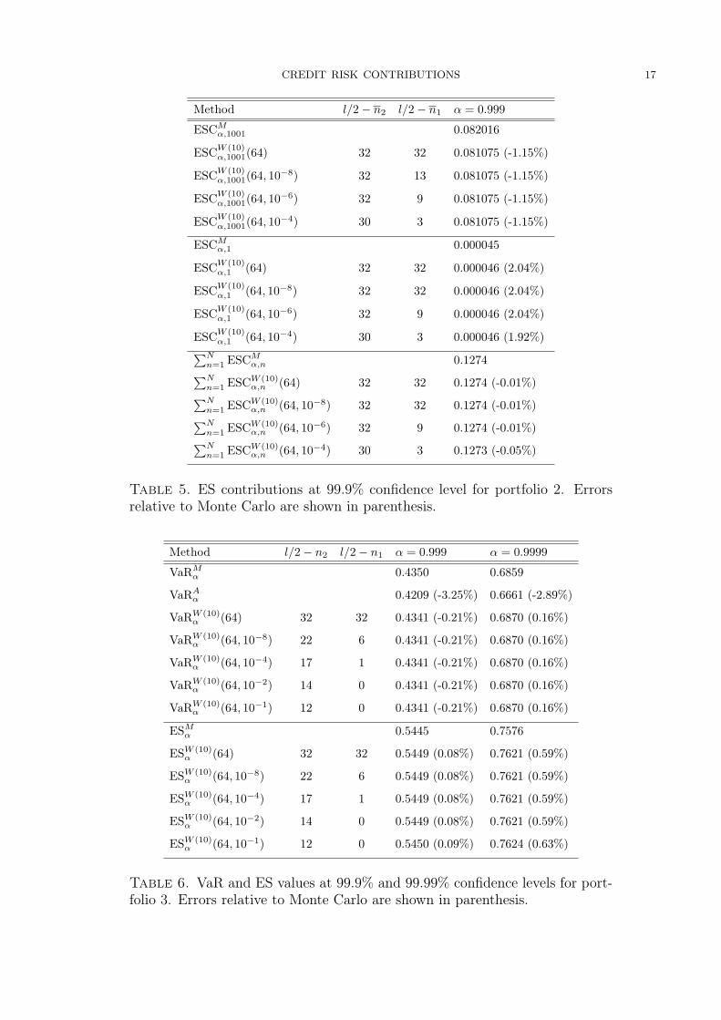
Method l/2− n2 l/2− n1 α = 0.999

ESCMα,1001 0.082016

ESCW (10)α,1001(64) 32 32 0.081075 (-1.15%)

ESCW (10)α,1001(64, 10−8) 32 13 0.081075 (-1.15%)

ESCW (10)α,1001(64, 10−6) 32 9 0.081075 (-1.15%)

ESCW (10)α,1001(64, 10−4) 30 3 0.081075 (-1.15%)

ESCMα,1 0.000045

ESCW (10)α,1 (64) 32 32 0.000046 (2.04%)

ESCW (10)α,1 (64, 10−8) 32 32 0.000046 (2.04%)

ESCW (10)α,1 (64, 10−6) 32 9 0.000046 (2.04%)

ESCW (10)α,1 (64, 10−4) 30 3 0.000046 (1.92%)∑N

n=1 ESCMα,n 0.1274∑N

n=1 ESCW (10)α,n (64) 32 32 0.1274 (-0.01%)∑N

n=1 ESCW (10)α,n (64, 10−8) 32 32 0.1274 (-0.01%)∑N

n=1 ESCW (10)α,n (64, 10−6) 32 9 0.1274 (-0.01%)∑N

n=1 ESCW (10)α,n (64, 10−4) 30 3 0.1273 (-0.05%)

Table 5. ES contributions at 99.9% confidence level for portfolio 2. Errorsrelative to Monte Carlo are shown in parenthesis.

Method l/2− n2 l/2− n1 α = 0.999 α = 0.9999

VaRMα 0.4350 0.6859

VaRAα 0.4209 (-3.25%) 0.6661 (-2.89%)

VaRW (10)α (64) 32 32 0.4341 (-0.21%) 0.6870 (0.16%)

VaRW (10)α (64, 10−8) 22 6 0.4341 (-0.21%) 0.6870 (0.16%)

VaRW (10)α (64, 10−4) 17 1 0.4341 (-0.21%) 0.6870 (0.16%)

VaRW (10)α (64, 10−2) 14 0 0.4341 (-0.21%) 0.6870 (0.16%)

VaRW (10)α (64, 10−1) 12 0 0.4341 (-0.21%) 0.6870 (0.16%)

ESMα 0.5445 0.7576

ESW (10)α (64) 32 32 0.5449 (0.08%) 0.7621 (0.59%)

ESW (10)α (64, 10−8) 22 6 0.5449 (0.08%) 0.7621 (0.59%)

ESW (10)α (64, 10−4) 17 1 0.5449 (0.08%) 0.7621 (0.59%)

ESW (10)α (64, 10−2) 14 0 0.5449 (0.08%) 0.7621 (0.59%)

ESW (10)α (64, 10−1) 12 0 0.5450 (0.09%) 0.7624 (0.63%)

Table 6. VaR and ES values at 99.9% and 99.99% confidence levels for port-folio 3. Errors relative to Monte Carlo are shown in parenthesis.


l/2−n

2l/

2−n

1j 1

=1,j

2=

20

j 1=

21,j

2=

40

j 1=

41,j

2=

60

j 1=

61,j

2=

80

j 1=

81,j

2=

100

MC

99%

CI

(-0.

0003

29,0

.001

073)

(0.0

0080

7,0.

0022

09)

(0.0

0271

0,0.

0041

12)

(0.0

0558

5,0.

0069

87)

(0.0

0947

3,0.

0108

75)

∑ j 2 j=

j1

VaR

CA 0

.999

,j

20

0.00

0383

0.00

1530

0.00

3443

0.00

6121

0.00

9565

∑ j 2 j=

j1

VaR

CW

(m)

0.9

99

,j(6

4)

20

3232

0.00

0364

0.00

1472

0.00

3435

0.00

6229

0.01

0203

∑ j 2 j=

j1

VaR

CW

(m)

0.9

99

,j(6

4,1

0−

8)

20

226

0.00

0364

0.00

1472

0.00

3435

0.00

6229

0.01

0203

∑ j 2 j=

j1

VaR

CW

(m)

0.9

99

,j(6

4,1

0−

6)

20

204

0.00

0364

0.00

1472

0.00

3435

0.00

6229

0.01

0203

∑ j 2 j=

j1

VaR

CW

(m)

0.9

99

,j(6

4,1

0−

4)

20

171

0.00

0364

0.00

1475

0.00

3442

0.00

6226

0.01

0197

Tabl

e7.

VaR

contribu

tion

sat

99.9%

confi

dencelevelforpo

rtfolio

3.The

values

presentedfortheVaR

contribu

tion

sha

vebe

enaverag

edover

grou

psof

oblig

orswiththesameexpo

sure.

l/2−n

2l/

2−n

1j 1

=1,j

2=

20

j 1=

21,j

2=

40

j 1=

41,j

2=

60

j 1=

61,j

2=

80

j 1=

81,j

2=

100

∑∑ j 2 j

=j1

ESC

M 0.9

99

,j

20

0.00

0466

0.00

1883

0.00

4316

0.00

7861

0.01

2677

0.54

41∑ j 2 j

=j1

ESC

W(1

0)

0.9

99

,j(6

4)

20

3232

0.00

0466

(-0.

06%

)0.

0018

84(0

.04%

)0.

0043

15(-

0.03

%)

0.00

7867

(0.0

8%)

0.01

2696

(0.1

5%)

0.54

46(0

.09%

)∑ j 2 j

=j1

ESC

W(1

0)

0.9

99

,j(6

4,1

0−

8)

20

226

0.00

0466

(-0.

06%

)0.

0018

84(0

.04%

)0.

0043

15(-

0.03

%)

0.00

7867

(0.0

8%)

0.01

2696

(0.1

5%)

0.54

46(0

.09%

)∑ j 2 j

=j1

ESC

W(1

0)

0.9

99

,j(6

4,1

0−

6)

20

204

0.00

0466

(-0.

06%

)0.

0018

84(0

.04%

)0.

0043

15(-

0.03

%)

0.00

7867

(0.0

8%)

0.01

2696

(0.1

5%)

0.54

46(0

.09%

)∑ j 2 j

=j1

ESC

W(1

0)

0.9

99

,j(6

4,1

0−

4)

20

171

0.00

0460

(-1.

38%

)0.

0018

84(0

.04%

)0.

0043

15(-

0.03

%)

0.00

7867

(0.0

8%)

0.01

2696

(0.1

5%)

0.54

44(0

.07%

)

Tabl

e8.

EScontribu

tion

sat

99.9%

confi

dencelevelfor

portfolio

3.The

values

presentedfortheEScontribu

tion

sha

vebe

enaverag

edover

grou

psof

oblig

orswiththesameexpo

sure.The

last

columnrepresents

thesum

ofallt

hecredit

risk

contribu

tion

s.Errorsrelative

toMon

teCarlo

areshow

nin

parenthesis.


l/2−n

2l/

2−n

1j 1

=1,j

2=

20

j 1=

21,j

2=

40

j 1=

41,j

2=

60

j 1=

61,j

2=

80

j 1=

81,j

2=

100

∑∑ j 2 j

=j1

ESC

M 0.9

999

,j

20

0.00

0662

0.00

2667

0.00

6094

0.01

1034

0.01

7705

0.76

32∑ j 2 j

=j1

ESC

W(1

0)

0.9

999

,j(6

4)

20

3232

0.00

0658

(-0.

51%

)0.

0026

57(-

0.38

%)

0.00

6067

(-0.

45%

)0.

0110

09(-

0.23

%)

0.01

7643

(-0.

35%

)0.

7607

(-0.

33%

)∑ j 2 j

=j1

ESC

W(1

0)

0.9

999

,j(6

4,1

0−

8)

20

226

0.00

0658

(-0.

51%

)0.

0026

57(-

0.38

%)

0.00

6067

(-0.

45%

)0.

0110

09(-

0.23

%)

0.01

7643

(-0.

35%

)0.

7607

(-0.

33%

)∑ j 2 j

=j1

ESC

W(1

0)

0.9

999

,j(6

4,1

0−

6)

20

204

0.00

0658

(-0.

51%

)0.

0026

57(-

0.38

%)

0.00

6067

(-0.

45%

)0.

0110

09(-

0.23

%)

0.01

7643

(-0.

35%

)0.

7607

(-0.

33%

)∑ j 2 j

=j1

ESC

W(1

0)

0.9

999

,j(6

4,1

0−

4)

20

171

0.00

0622

(-5.

93%

)0.

0026

57(-

0.38

%)

0.00

6067

(-0.

45%

)0.

0110

09(-

0.23

%)

0.01

7643

(-0.

35%

)0.

7600

(-0.

43%

)

Tabl

e9.

EScontribu

tion

sat

99.99%

confi

dencelevelfor

portfolio

3.The

values

presentedfortheEScontribu

tion

sha

vebe

enaverag

edover

grou

psof

oblig

orswiththesameexpo

sure.The

last

columnrepresents

thesum

ofallt

hecredit

risk

contribu

tion

s.Errorsrelative

toMon

teCarlo

areshow

nin

parenthesis.


1.E-05

1.E-04

1.E-03

1.E-02

1.E-01

1.E+00

0.00 0.10 0.20 0.30 0.40 0.50 0.60 0.70 0.80 0.90 1.00

Loss level

Tail p

rob

ab

ilit

y

MC WA ASRF

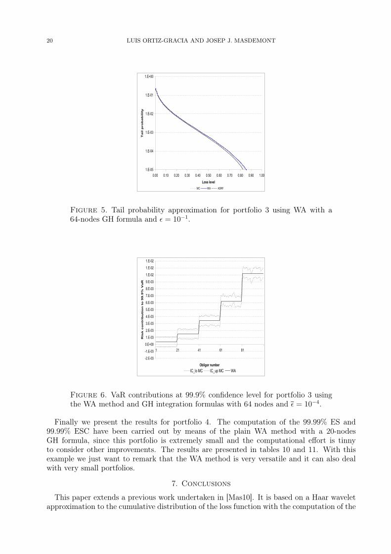
Figure 5. Tail probability approximation for portfolio 3 using WA with a64-nodes GH formula and ε = 10−1.

-2.E-03

-1.E-03

0.E+00

1.E-03

2.E-03

3.E-03

4.E-03

5.E-03

6.E-03

7.E-03

8.E-03

9.E-03

1.E-02

1.E-02

1.E-02

1 21 41 61 81

Obligor number

Ris

k c

on

trib

uti

on

to

99.9

% V

aR

IC_lo MC IC_up MC WA

Figure 6. VaR contributions at 99.9% confidence level for portfolio 3 usingthe WA method and GH integration formulas with 64 nodes and ε = 10−4.

Finally we present the results for portfolio 4. The computation of the 99.99% ES and99.99% ESC have been carried out by means of the plain WA method with a 20-nodesGH formula, since this portfolio is extremely small and the computational effort is tinnyto consider other improvements. The results are presented in tables 10 and 11. With thisexample we just want to remark that the WA method is very versatile and it can also dealwith very small portfolios.

7. Conclusions

This paper extends a previous work undertaken in [Mas10]. It is based on a Haar waveletapproximation to the cumulative distribution of the loss function with the computation of the


-1.E-03

4.E-03

9.E-03

1.E-02

1 21 41 61 81Obligor number

Ris

k c

on

trib

uti

on

to

99

.9%

ES


-1.E-03

4.E-03

9.E-03

1.E-02

2.E-02

1 21 41 61 81Obligor number

Ris

k c

on

trib

uti

on

to

99.9

9%

ES


Figure 7. Expected Shortfall contributions at 99.9% (left) and 99.99% (right)confidence levels for portfolio 3 using the WA method and GH integrationformulas with 64 nodes and ε = 10−4.

Method α = 0.9999

ESMα 0.6833

ESW (10)α (20) 0.6814 (-0.29%)

Table 10. ES at 99.99% confidence level for portfolio 4. Relative error toMonte Carlo is shown in parenthesis.

ES as an alternative coherent risk measure to VaR. Moreover, a detailed procedure for thecalculation of the risk contributions to the VaR and the ES in a credit portfolio is provided.The risk contributions are known to be very computationally intensive to be estimated bymeans of MC because they are the expected value of the individual loss conditioned on arare event. Therefore, analytical or fast numerical methods are welcome to overcome thisproblem. The model framework is the well known Vasicek one-factor model, a one-perioddefault model, which is the basis of the Basel II Accord.

There are technical points taken into account that contribute to a considerable improve-ment of the WA method. We avoid the evaluation of the MFG in all the nodes of theGauss-Hermite formulas by means of using its asymptotic behavior. Proceeding this way thespeed of the WA method increases while accuracy is even improved with the choice of theparameter r. These improvements are also applied to the computation of risk contributionsto VaR and ES, although the impact in the speed of the algorithm is much more relevant forrisk measures than for risk contributions.

This new methodology has been tested in a wide sized variety of portfolios, all them withexposure concentration, where the Asymptotic Single Risk Factor Model fails due to thename concentration. The results presented show that the Wavelet Approximation method ishighly competitive in terms of robustness, speed and accuracy being a very suitable methodto measure and manage the risks that arise in credit portfolios of financial companies.


Obligor ESCW (10)0.9999,n(20) ESCM0.9999,n Relative error

1 0.340472 0.338706 0.52%

2 0.128672 0.128885 -0.17%

3 0.059568 0.059426 0.24%

4 0.041619 0.042070 -1.07%

5 0.028044 0.028805 -2.64 %

6 0.023233 0.022825 1.79%

7 0.019335 0.019348 -0.06%

8 0.016606 0.015935 4.21%

9 0.014527 0.014614 -0.60%

10 0.012971 0.012227 6.08%∑Nn=1 ESC

W (10)0.9999,n(20) 0.6850 0.6828 0.32%

Table 11. ES contributions at 99.99% confidence level for portfolio 4 withthe WA method.

References

[Art99] P. Artzner, F. Delbaen, J.M. Eber, D. Heath (1999). Coherent measures of risk. Mathematical Finance9 (3): 203-228.

[Gla05] P. Glasserman (2005). Measuring marginal risk contributions in credit portfolios. Journal of Com-putational Finance. V. 9, N. 2, 1-41.

[Hua07a] X. Huang, C. W. Oosterlee and J. A. M. van der Weide (2007). Higher-order saddlepoint ap-proximations in the Vasicek portfolio credit loss model. Journal of Computational Finance V. 11, N. 1,93-113.

[Hua07b] X. Huang, C. W. Oosterlee and M. A. M. Mesters (2007). Computation of VaR and VaR contri-bution in the Vasicek portfolio credit loss model. Journal of Credit Risk V. 3, N. 3, 75-96.

[Lut09] E. Lütkebohmert (2009). Concentration risk in credit portfolios. Springer.[Mar01a] R. Martin, K. Thompson and C. Browne (2001). Taking to the saddle. RISK (June), 91-94.[Mar01b] R. Martin, K. Thompson and C. Browne (2001). VaR: who contributes and how much?. RISK

(August), 99-102.[Mas10] J. J. Masdemont and L. Ortiz-Gracia (2010). Haar wavelets-based approach for quantifying credit

portfolio losses. Available at www.crm.cat.[Tak08] Y. Takano and J. Hashiba (2008). A novel methodology for credit portfolio analysis: numerical

approximation approach. Available at www.defaultrisk.com.[Tas00] D. Tasche (2000). Risk contributions and performance measurement. Working paper, Munich Uni-

versity of Technology.


Luis Ortiz-GraciaCentre de Recerca MatemàticaCampus de Bellaterra, Edifici C08193 Bellaterra(Barcelona), Spain

E-mail address: [email protected]

Josep J. MasdemontDepartament de Matemàtica Aplicada IUniversitat Politècnica de CatalunyaDiagonal 64708028 Barcelona, Spain

E-mail address: [email protected]

credit risk contributions under the vasicek one-factor ... · credit risk contributions under the...

Documents