credit risk model building steps
TRANSCRIPT

Credit Risk Model Building StepsVenkat Reddy

Disclaimer
• This presentation is just the class notes. The best way to treat this is as a high-level summary;
• The actual session went more in-depth and contained other information.
• Most of this material was written as informal notes, not intended for publication
• Prerequisites:
• Basic knowledge of Credit Risk and Predictive modeling
• Practical Business Analytics Using SAS: A Hands-on Guide http://www.amazon.com/Practical-Business-Analytics-Using-Hands/dp/1484200446
Cre
dit
Ris
k M
od
el B
uild
ing
Ven
kat
Red
dy
2

Credit Risk Model Building StepsObjective
Exclusions
Observation point and/or window
Performance window
Bad definition
Segmentation
Variable selection
Regression Line
Model validation
Model recalibration
Cre
dit
Ris
k M
od
el B
uild
ing
Ven
kat
Red
dy
3

Credit Risk Model Building StepsObjective
Exclusions
Observation point and/or window
Performance window
Bad definition
Segmentation
Variable selection
Regression Line
Model validation
Model recalibration
Cre
dit
Ris
k M
od
el B
uild
ing
Ven
kat
Red
dy
4

Initial Discussions
Do we need a model? What type of model?
Issue, portfolio size, performance, growth plans, competitive and
economic environment
Can we build a model?
Data availability and integrity, legal/regulatory environment
Can we implement a model?
Project management and system development resources
Can we use the model in a strategy?
What decision can we make differently by using score
Can we prioritize the model in regional plan?
Evaluate the capacity of regional plan and the necessity of the model
Cre
dit
Ris
k M
od
el B
uild
ing
Ven
kat
Red
dy
5

Initial Discussions
Project Objectives
• Business Issue and Size of Problem/Driver for Score Development, Potential Strategic Score Uses, Estimated Project Impact (NCL, collection expenses, revenue, others)
Business Overview
• Products, Target Market, Economic Environment, Cultural Influences, Product Features and MIS, Collection and Other Policies, Existing Scores
Data Availability and Implementation Restrictions
• Data Files and Systems, File Layouts and Data Dictionaries
Cre
dit
Ris
k M
od
el B
uild
ing
Ven
kat
Red
dy
6

Scope of Score
• Customer Score vs Account Score
• Often in the use of the day to day operation the business prefer to have a customer view not an account view. Why ?
• Scope of the score
• Be clear about the objective of the score. Information about the scope of the score and the product business operation should be collected during project initiation.
• For ECM and collections scores all the customer accounts data is used during development. Why? and why only for ECM and collections
Cre
dit
Ris
k M
od
el B
uild
ing
Ven
kat
Red
dy
7

Credit Risk Model Building StepsObjective
Exclusions
Observation point and/or window
Performance window
Bad definition
Segmentation
Variable selection
Regression Line
Model validation
Model recalibration
Cre
dit
Ris
k M
od
el B
uild
ing
Ven
kat
Red
dy
8
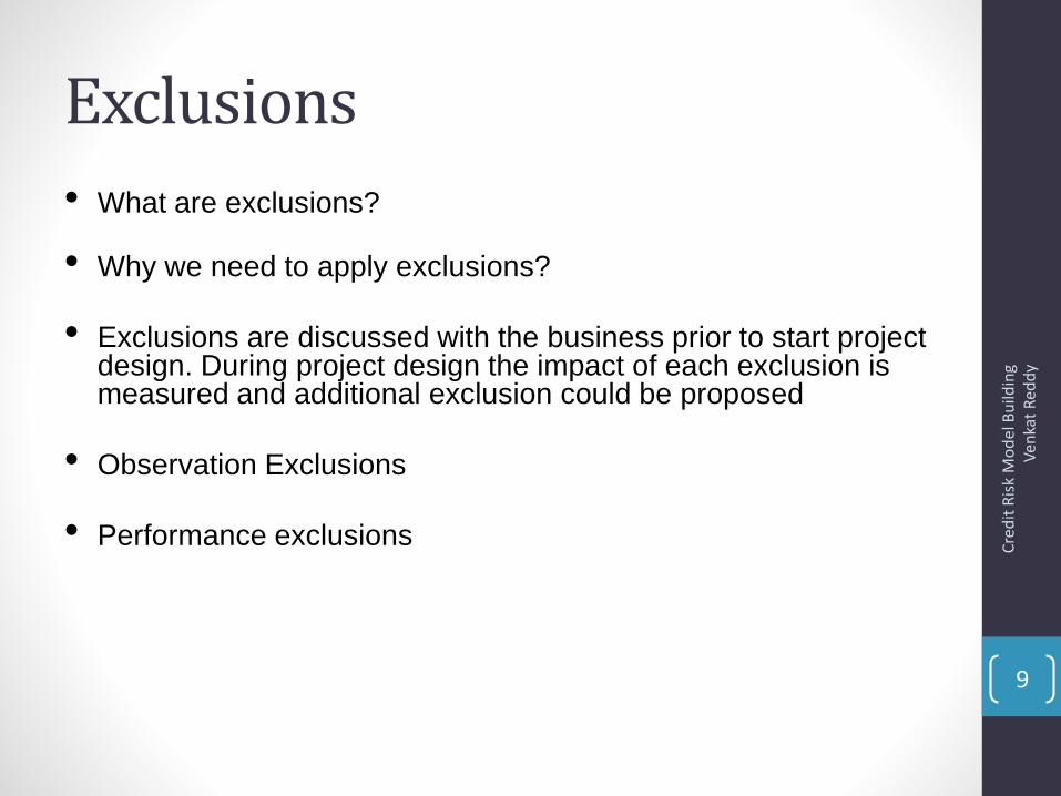
Exclusions
• What are exclusions?
• Why we need to apply exclusions?
• Exclusions are discussed with the business prior to start project design. During project design the impact of each exclusion is measured and additional exclusion could be proposed
• Observation Exclusions
• Performance exclusions Cre
dit
Ris
k M
od
el B
uild
ing
Ven
kat
Red
dy
9

Exclusions…..examples
• Possible Observation Period Exclusions
• Fraud cases
• Credit policy deviations that can include age, income, loan amount, debt burden, tenure etc.
• Credit Policy Fatal Criteria
• Test Accounts (what are these?)
• Possible Performance Exclusions
• Fraud Cases
• Deceased customers
• Indeterminate
Cre
dit
Ris
k M
od
el B
uild
ing
Ven
kat
Red
dy
10

Credit Risk Model Building StepsObjective
Exclusions
Observation point and/or window
Performance window
Bad definition
Segmentation
Variable selection
Regression Line
Model validation
Model recalibration
Cre
dit
Ris
k M
od
el B
uild
ing
Ven
kat
Red
dy
11

Observation Point
• Observation Point :Time period used to define the modeling population/ sample.
• The period needs to be representative of the current/future scoring environment.
• Only variables showing applicant/account behavior or characteristics at time of observation or prior to that can be used in model development. Why?
Observation Point
History Performance window
Cre
dit
Ris
k M
od
el B
uild
ing
Ven
kat
Red
dy
12

Performance window
What is performance window?
Key factors in choosing Performance period are :
Window should be long enough to ensure accounts have sufficient time for their
performance to mature
Sufficient number of goods and bads are there
Choosing optimal performance window could be done using Vintage
Analysis.
Cre
dit
Ris
k M
od
el B
uild
ing
Ven
kat
Red
dy
13

Vintage Analysis to decide Performance window
• Minimum number of months required to capture the default • How much time does it take to get defaulted • Look at the previous delinquencies for the accounts
Cre
dit
Ris
k M
od
el B
uild
ing
Ven
kat
Red
dy
14

30+ DPD % Account By Vintage and MOB
• 30+ DPD Count is getting stabilized at MOB 18
Cre
dit
Ris
k M
od
el B
uild
ing
Ven
kat
Red
dy
15

60+ DPD % Account By Vintage and MOB
60+ DPD is getting stabilized at MOB 18
Cre
dit
Ris
k M
od
el B
uild
ing
Ven
kat
Red
dy
16

90+ DPD Count By Vintage and MOB
• 90+ DPD is getting stabilized at MOB 18
Cre
dit
Ris
k M
od
el B
uild
ing
Ven
kat
Red
dy
17

Vintage analysis-Conclusion
• For Counts , the peak is occurring at 7 MOB for 30+, at 8 MOB for 60+ and 9 MOB for 90+.
• For Counts, there are peaks at 16, 28, 40 MOB for 30+. Similarly, these peaks occur for 60+ and 90+ at 17, 29, 41 MOB and 18 , 30, 42 MOB respectively.
• Peak delinquency followed by stable delinquency rates occur within the first 18 months of performance.
• So the performance window is 18 months
Cre
dit
Ris
k M
od
el B
uild
ing
Ven
kat
Red
dy
18

Lab: Vintage Analysis
• Download Credit Risk Vintage Data
• Draw 30+ DPD, 60+ DPD, 90+DPD graphs
• Write your observations
• What is the peak month with respect to delinquencies?
• Decide the performance window
Cre
dit
Ris
k M
od
el B
uild
ing
Ven
kat
Red
dy
19

Model Building stepsObjective
Exclusions
Observation point and/or window
Performance window
Bad definition
Segmentation
Variable selection
Regression Line
Model validation
Model recalibration
Cre
dit
Ris
k M
od
el B
uild
ing
Ven
kat
Red
dy
20

‘Bad’ Definition
• Bankruptcy is the only form of bad?
• Can 160+ delinquent be bad?
• A customer or a loan is bad when, due to lack of repayment, the customer or loan must to be charged off.
• Typically, the concern is to catch the “MOST BAD” account in the shortest performance window.
Cre
dit
Ris
k M
od
el B
uild
ing
Ven
kat
Red
dy
21

‘Bad’ Definition
• So what should we use as “BAD”?
• Ask the business how they define bad as they need to be comfortable with the definition.
• Perform some analysis to confirm that the business’ perception of bad is accurate:
• Roll rate analysis and waterfall analysis
• Re-write and re-aging analysis
Cre
dit
Ris
k M
od
el B
uild
ing
Ven
kat
Red
dy
22

Bad definition
Cre
dit
Ris
k M
od
el B
uild
ing
Ven
kat
Red
dy
23
No Due 90,000
30 days due 40,000
60 days due 20,000
90 days due 10,000
120 days due 6,000
150 days due 2,000
180 days due -BK 1,000
Start of the performance window
No Due 30 days due 60 days due 90 days due 120 days due 150 days due 180 days due -BK
No Due 78,300 4,500 3,150 1,800 1,350 630 270 90,000
30 days due 30,800 4,000 2,200 1,200 1,000 480 320 40,000
60 days due 13,400 3,000 2,100 400 300 140 660 20,000
90 days due 3,700 2,500 1,350 200 950 770 530 10,000
120 days due 1,620 480 300 120 420 1,842 1,218 6,000
150 days due 340 100 70 40 30 514 906 2,000
180 days due -BK 30 20 10 5 3 4 928 1,000
End- After 18 Months

Calculation of Bad
Cre
dit
Ris
k M
od
el B
uild
ing
Ven
kat
Red
dy
24
No Due 30 days due 60 days due 90 days due 120 days due 150 days due 180 days due -BK Rollback Roll Forward
No Due 87.0% 5.0% 3.5% 2.0% 1.5% 0.7% 0.3% 013.0%
30 days due 77.0% 10.0% 5.5% 3.0% 2.5% 1.2% 0.8% 77.0%13.0%
60 days due 67.0% 15.0% 10.5% 2.0% 1.5% 0.7% 3.3% 82%7.5%
90 days due 37.0% 25.0% 13.5% 2.0% 9.5% 7.7% 5.3% 76%22.5%
120 days due 27.0% 8.0% 5.0% 2.0% 7.0% 30.7% 20.3% 42%51.0%
150 days due 17.0% 5.0% 3.5% 2.0% 1.5% 25.7% 45.3% 29%45.3%
180 days due -BK 3.0% 2.0% 1.0% 0.5% 0.3% 0.4% 92.8% 7%0.0%
End- After 18 Months
• How many people are 120+ dpd at the start of the year?
• How may people out them jumped below 120+ bucket ( current/ 30+/60+/90+) how may people are above 120+ (150+/180+)
• From the Flow Rate Analysis we can segment the population in 2 segments.

Bad Definition- Example
Count % Cum% Current %
Current
due % X-DPD %
30-59
DPD %
60-89
DPD %
90-119
DPD %
120-149
DPD %
150-
179
DPD %
180+DP
D %
Current 26637 46.36% 46.36% 20364 76.45% 3806 14.29% 1821 6.84% 333 1.25% 150 0.56% 74 0.28% 45 0.17% 44 0.17% 0.00%
Current
due 20402 35.50% 81.86% 4683 22.95% 12632 61.92% 2330 11.42% 425 2.08% 161 0.79% 84 0.41% 51 0.25% 36 0.18% 0.00%
X-DPD 6544 11.39% 93.25% 2003 30.61% 1831 27.98% 1554 23.75% 531 8.11% 250 3.82% 149 2.28% 96 1.47% 66 1.01% 64 0.98%
30-59
DPD 1255 2.18% 95.43% 335 26.69% 183 14.58% 183 14.58% 149 11.87% 107 8.53% 83 6.61% 59 4.70% 54 4.30% 102 8.13%
60-89
DPD 601 1.05% 96.48% 162 26.96% 35 5.82% 62 10.32% 40 6.66% 41 6.82% 30 4.99% 38 6.32% 48 7.99% 145 24.13%
90-119
DPD 383 0.67% 97.14% 117 30.55% 14 3.66% 15 3.92% 14 3.66% 14 3.66% 27 7.05% 27 7.05% 26 6.79% 129 33.68%
120-149
DPD 357 0.62% 97.77% 96 26.89% 8 2.24% 12 3.36% 7 1.96% 8 2.24% 14 3.92% 30 8.40% 17 4.76% 165 46.22%
150-179
DPD 308 0.54% 98.30% 49 15.91% 1 0.32% 14 4.55% 7 2.27% 6 1.95% 13 4.22% 9 2.92% 56 18.18% 153 49.68%
180+DPD 976 1.70% 100.00% 44 4.51% 4 0.41% 33 3.38% 11 1.13% 6 0.61% 4 0.41% 18 1.84% 24 2.46% 832 85.25%
Performance at the end of 12th MOB Performance at the end of 18th MOB
• How many people are 90+ dpd at the start of the year?
• How may people out them jumped below 90+ bucket ( current/ 30+/60+) how may people are above 90+ (120+/150+/180+)
• From the Flow Rate Analysis we can segment the population in 3 segments.
• Good: Current, Current due, X-DPD at the end of 12 month
• Indeterminate: 30-59 DPD at the end of 12 month
• Bad:60+DPD at the end of 12 month
Cre
dit
Ris
k M
od
el B
uild
ing
Ven
kat
Red
dy
25

Indeterminate
• Example:
• BAD: 90 or worse in the performance window
• Indeterminate: 30+ but never worse in the performance window
• Good: not bad or indeterminate
• In general, It is not advised to have a indeterminate group bigger than 20% of the total sample.
• Observations flagged as indeterminate are excluded from the modeling sample (performance exclusion). Why?
• Defining an indeterminate population can help to show a higher KS (exclude grey keep only black and white).
Cre
dit
Ris
k M
od
el B
uild
ing
Ven
kat
Red
dy
26

Lab: Bad definition
• Download ‘bad_definition.xls’
• How many accounts are we studying in this example?
• How may accounts are current?
• How many of these are 90+ dpd at the start
• Interpret the water fall analysis
• What can be bad definition
• Give definition for good & Indeterminate
• How do you decide indeterminate? Cre
dit
Ris
k M
od
el B
uild
ing
Ven
kat
Red
dy
27

Model Building stepsObjective
Exclusions
Observation point and/or window
Performance window
Bad definition
Segmentation
Variable selection
Regression Line
Model validation
Model recalibration
Cre
dit
Ris
k M
od
el B
uild
ing
Ven
kat
Red
dy
28

Segmentation
“One size does not fit all”
• “Separating good from bad” - Is this the objective of segmentation?
• Not directly, but segmentation allows different scorecards to be built for each population, which in turn leads to better separation of goods from the bads better than a single scorecard could, thus improving overall accuracy.
Cre
dit
Ris
k M
od
el B
uild
ing
Ven
kat
Red
dy
29

Segmentation Variables Product types ( since usually different product variations are targeted at different
sub-sections of the population) Platinum / Silver / Gold Credit Cards Store Cards / Bank Cards Secured / Unsecured Loans New vs. Refinanced Auto Loans Fixed Rate / Adjustable Rate Mortgages Fixed / Revolving Home Equity Line of Credit
Length / tenure of close ended product ( esp. applicable for installment products) Month on Book on Bureau (Thin / Thick File ) Clean / Dirty File Different portfolios
Consumer / Commercial Oil / Financial Institutions / Business / Professional Institutions Existing Customers / Former Customers / New Customers
Demographics Regional / Age / Income / Lifestyle attributes
Channel Prescreen mailing / Telemarketing / Email campaign
Type of Customer New / Former / Existing
Cre
dit
Ris
k M
od
el B
uild
ing
Ven
kat
Red
dy
30

When to segment?
• When it will improve the score’s ability to separate goods from bads
• When population is made up of distinct subpopulations
• When there is a business need to do so
• When segmented scorecards perform significantly better than single scorecard
• When incremental cost of using multiple scorecards is significantly less
• When the interactive variable approach is not feasible
“The gain from segmentation should be substantial before a developer opts for it”
Cre
dit
Ris
k M
od
el B
uild
ing
Ven
kat
Red
dy
31

Types of segmentation
1.Strategic
2.Operational
3.Statistical
• A lender strategically targeting a certain group of customers
• eg. Borrowers who are already in the books of the lender on a different line of credit
• Availability of different data sources for different customer segments
• eg. Origination through bank branch or third party origination
• Some characteristics affecting the outcome variable differently for some population
• eg. Effect of serious delinquency on a thin-file vs thick-file applicant
Cre
dit
Ris
k M
od
el B
uild
ing
Ven
kat
Red
dy
32

Model Building stepsObjective
Exclusions
Observation point and/or window
Performance window
Bad definition
Segmentation
Variable selection
Regression Line
Model validation
Model recalibration
Cre
dit
Ris
k M
od
el B
uild
ing
Ven
kat
Red
dy
33

What is variable selection?
• We have historical data of 10,000 customers. There are two variables income class, distance from bank
• What is the difference between these two variables?
• Which one is important ?
Income Good Bad
Very High 1990 10
High 1960 40
Medium 1900 100
Low 1850 150
Very Low 1300 700
9000 1000
Distance Good Bad
Very far 1800 200
Far 1800 200
Medium 1800 200
Not far 1800 200
Very near 1800 200
9000 1000
• As income increase what happens to number of bad?• As distance increases what happens to number of bad?
Cre
dit
Ris
k M
od
el B
uild
ing
Ven
kat
Red
dy
34

Which variable to select?
The Model building exercise is all about selecting an optimal combination of variables, from a given list of all the variables, which will be able to predict moderately if an account is good or bad.
x11
x7x2
x8
x6
x12
x9x1 x10
x13
x5x4
x3
Good
Bad
Var- x11
Good
Bad
Var- x7
Cre
dit
Ris
k M
od
el B
uild
ing
Ven
kat
Red
dy
35
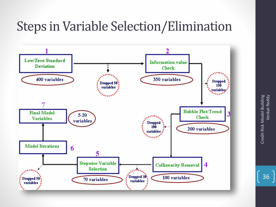
Steps in Variable Selection/Elimination
Cre
dit
Ris
k M
od
el B
uild
ing
Ven
kat
Red
dy
36

Types of variables
Payment History
• Account payment information on specific types of accounts (credit cards, retail accounts, installment loans, finance company accounts, mortgage, etc.)
• Presence of adverse public records (bankruptcy, judgements, suits, liens, wage attachments, etc.), collection items, and/or delinquency (past due items)
• Severity of delinquency (how long past due)
• Amount past due on delinquent accounts or collection items
• Time since (recency of) past due items (delinquency), adverse public records (if any), or collection items (if any)
• Number of past due items on file
• Number of accounts paid as agreed
Cre
dit
Ris
k M
od
el B
uild
ing
Ven
kat
Red
dy
37

List of variables
Amounts Owed
• Amount owing on accounts
• Amount owing on specific types of accounts
• Lack of a specific type of balance, in some cases
• Number of accounts with balances
• Proportion of credit lines used (proportion of balances to total credit limits on certain types of revolving accounts)
• Proportion of installment loan amounts still owing (proportion of balance to original loan amount on certain types of installment loans)
Cre
dit
Ris
k M
od
el B
uild
ing
Ven
kat
Red
dy
38

List of variables
Length of Credit History• Time since accounts opened• Time since accounts opened, by specific type of account• Time since account activityNew Credit• Number of recently opened accounts, and proportion of accounts
that are recently opened, by type of account• Number of recent credit inquiries• Time since recent account opening(s), by type of account• Time since credit inquiry(s)• Re-establishment of positive credit history following past payment
problemsTypes of Credit Used• Number of (presence, prevalence, and recent information on)
various types of accounts (credit cards, retail accounts, installment loans, mortgage, consumer finance accounts, etc.)
Cre
dit
Ris
k M
od
el B
uild
ing
Ven
kat
Red
dy
39

Variable Selection-Drop inconsistent variables
• Before going to different statistical methods of variable selection, we remove inconsistent variables from data.
• Variables with all missing or high percentages (as > 90%) of missing should be discarded.
• Variables with single value (or standard deviations as 0) should be discarded. (Any other examples?)
• Variables with infinite variance, unique to each account(mobile number etc.,)
Cre
dit
Ris
k M
od
el B
uild
ing
Ven
kat
Red
dy
40

Variable Selection-Information Value
• Which variable to keep and which one to drop in above examples?
• How to quantify this effect?
• Measuring the trend using a mathematical formula?
Income Good Bad
Very High 1990 10
High 1960 40
Medium 1900 100
Low 1850 150
Very Low 1300 700
9000 1000
Distance Good Bad
Very far 1800 200
Far 1800 200
Medium 1800 200
Not far 1800 200
Very near 1800 200
9000 1000
Cre
dit
Ris
k M
od
el B
uild
ing
Ven
kat
Red
dy
41

Information Value-Example
• The relative risk of the attribute is determined by its “Weight of Evidence.”
%Good %Bad
[x] [Y]
< 5 1850 150 29% 5% 6.31 0.25 0.80 0.20
5-30 1600 400 25% 12% 2.05 0.13 0.31 0.04
31 - 60 1200 600 19% 18% 1.02 0.00 0.01 0.00
60 - 90 900 900 14% 28% 0.51 (0.14) -0.29 0.04
>= 91 800 1200 13% 37% 0.34 (0.24) -0.47 0.11
Total 6350 3250 0.39
WOE = Log
(X/Y)IV
Utilizatio
n %
# of
Good# of Bad
%Good
/ %BadX -Y
Cre
dit
Ris
k M
od
el B
uild
ing
Ven
kat
Red
dy
42

Demo : Calculation of IV
0% 4,948 9,870
10% 6,400 8,956
20% 7,203 7,869
30% 8,679 7,045
40% 9,345 6,800
50% 10,983 5,934
60% 11,673 5,021
70% 13,457 4,356
80% 14,000 3,004
90% 14,689 2,890
Utilization Good Bad
Cre
dit
Ris
k M
od
el B
uild
ing
Ven
kat
Red
dy
43

Rules of Thumb for selecting variable with the help of IV
• IF IV < 0.01 => very weak, discard the variable;
• ELSE IF IV < 0.1 => weak, variable can be included ;
• ELSE IF IV < 0.3 => medium, should be included;
• ELSE IF IV < 0.5 => strong, must be included
• ELSE IF >= 0.5 => the characteristic may be over-predicting, meaning that it is in some form trivially related to the good/bad information, check for the variable
Cre
dit
Ris
k M
od
el B
uild
ing
Ven
kat
Red
dy
44

Lab: WOE & IV
• Download Information value data
• Find IV of the variable “Number of enquiries”
• As number of enquiries increase what happens to bad rate?
• Find IV for “number of cards”
• As number of cards increase what happens to bad rate?
Cre
dit
Ris
k M
od
el B
uild
ing
Ven
kat
Red
dy
45

Steps in Variable Selection/Elimination
Cre
dit
Ris
k M
od
el B
uild
ing
Ven
kat
Red
dy
46

Bi-variate Trend Analysis
• After short listing variables based on information value, we perform trend analysis to check if the variables we want to include in the model having proper tend or not.
• Bivariate Trend Analysis is an analysis to check the trend of a variable with respect to the bad rates (i.e. what is the trend of bad-rate if the value of the variable increases) and accordingly include / exclude variables in the model
• What is the need of bivariate analysis?
• To identify the variable where, IV is high but variable is good for nothing C
red
it R
isk
Mo
del
Bu
ildin
g
V
enka
t R
edd
y
47

Log odd graphNum_Enq Good Bad %good %bad %g-%b %g/%b ln(%g/%b) IV
0 6400 150 17% 3% 14% 5.97 1.79 0.25
1 5800 169 15% 3% 12% 4.80 1.57 0.19
2 5445 340 14% 6% 8% 2.24 0.81 0.06
3 4500 250 12% 5% 7% 2.52 0.92 0.07
4 4070 375 11% 7% 4% 1.52 0.42 0.02
5 3726 470 10% 9% 1% 1.11 0.10 0.00
6 2879 650 8% 12% -5% 0.62 -0.48 0.02
7 1893 876 5% 17% -12% 0.30 -1.20 0.14
8 1636 987 4% 19% -14% 0.23 -1.46 0.21
9 1354 1008 4% 19% -16% 0.19 -1.67 0.26
37703 5275 1.22
Cre
dit
Ris
k M
od
el B
uild
ing
Ven
kat
Red
dy
48

Demo: Bivariate graph
• Number of dependents
Cre
dit
Ris
k M
od
el B
uild
ing
Ven
kat
Red
dy
49

Lab: Bivariate graph
• Draw log odds graph for Number of enquiries
• Draw log odds graph for Number of cards
Cre
dit
Ris
k M
od
el B
uild
ing
Ven
kat
Red
dy
50

Rules of Thumb for selecting variable with the help of trend chart
• Include Variable in the model if trend plot shows
• the trend following business intuition
• Exclude Variable from the model if plot shows
• opposite trend from business point of view.
• no trend / completely random plot. As no trend implies with the increase
in the variables value, there is no / random change in good (and hence
log(odds)) and hence the variable cannot be used to discriminate good
from bad. Hence variable should be dropped.
• Include variable with some adjustment if plot shows
• If a variable has a appropriate trend for most of the values and erratic in
the extreme values; do capping / flooring and include the variable in the
model if after capping / flooring the variable has a correct trend.
• monotonic but non-linear trend; such that after some transformation
e.g. Log transform, exponential transformation etc. the variable follows a
proper linear trend
Cre
dit
Ris
k M
od
el B
uild
ing
Ven
kat
Red
dy
51

Lab: Bi-variate Trend Analysis
• Download Information value data
• Find IV of the variable “Number of enquiries”
• Draw bivariate chart
• Find IV for “number of cards”
• Draw the bivariate chart
• As number of cards increase what happens to bad rate?
• Can we keep both variables in the model? Which one to keep? Which one to drop?
• Draw bivariate chart for utilization
Cre
dit
Ris
k M
od
el B
uild
ing
Ven
kat
Red
dy
52

Steps in Variable Selection/Elimination
Cre
dit
Ris
k M
od
el B
uild
ing
Ven
kat
Red
dy
53

Stepwise Regression
• Forward selection
• Backward elimination
• Stepwise Regression
Cre
dit
Ris
k M
od
el B
uild
ing
Ven
kat
Red
dy
54

Forward selection
1. Start with a null model
2. Add one variable at a time, record adj R-Square(or AIC). See if there is any significant increment in the adj R-square(or AIC)
• If there is significant increment then retain the variables
• If there is no significant increment then drop the variable
3. Repeat step-2 for all the variables
Cre
dit
Ris
k M
od
el B
uild
ing
Ven
kat
Red
dy
55

Backward elimination
1. Start with the full model with k variables
2. Remove variables one at a time, record adj R-Square(or AIC). See if there is any significant dip in adj R-square(or AIC)
• If there is significant dip then retain the variables
• If there is no significant dip then drop the variable
3. Repeat step-2 for all the variables
Cre
dit
Ris
k M
od
el B
uild
ing
Ven
kat
Red
dy
56

Stepwise regression
• Combination of FS & BE
• Start with null model
• Repeat:
• one step of FS
• one step of BE
• Stop when no improvement in Adj R-square or AIC is possible
Cre
dit
Ris
k M
od
el B
uild
ing
Ven
kat
Red
dy
57

Demo: Stepwise regression
• Contact center Customer satisfaction data
• C-Sat vs. Communication, Resolution,Attitude, Handling Time score
Cre
dit
Ris
k M
od
el B
uild
ing
Ven
kat
Red
dy
58

Lab: Stepwise Regression
• Import 8.3 Stepwise Regression_fraud.csv
• Print the contents
• Build a logistic regression line to predict the fraud
• Use stepwise regression to select/eliminate variables
Cre
dit
Ris
k M
od
el B
uild
ing
Ven
kat
Red
dy
59

Steps in Variable Selection/Elimination
Cre
dit
Ris
k M
od
el B
uild
ing
Ven
kat
Red
dy
60
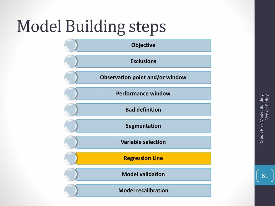
Model Building stepsObjective
Exclusions
Observation point and/or window
Performance window
Bad definition
Segmentation
Variable selection
Regression Line
Model validation
Model recalibration
Cre
dit
Ris
k M
od
el B
uild
ing
Ven
kat
Red
dy
61

Regression Line
• Logistic regression line
• Good/Bad on list of variables
Cre
dit
Ris
k M
od
el B
uild
ing
Ven
kat
Red
dy
62

Demo regression line
proc logistic data=mylib.Sample_cc descending;
model
SeriousDlqin2yrs=
util
age1
DebtRatio1
MonthlyIncome1
num_loans
depend
/ selection=stepwise ;
output out = mylib.lect_logit p=prob ;
run;
Cre
dit
Ris
k M
od
el B
uild
ing
Ven
kat
Red
dy
63

Model Building stepsObjective
Exclusions
Observation point and/or window
Performance window
Bad definition
Segmentation
Variable selection
Regression Line
Model validation
Model recalibration
Cre
dit
Ris
k M
od
el B
uild
ing
Ven
kat
Red
dy
64

What is the need of model validation?
Mar-2012
• 100,000 applications for loan
Population
• We build a model to decide the score
Scorecard• We approved and
rejected applications based on the score
Approval
Mar-2013
• 125,000 applications for loan
Population
• ?
Scorecard• ?
Approval
Cre
dit
Ris
k M
od
el B
uild
ing
Ven
kat
Red
dy
65

What is the need of model validation?
• To make sure that the old model is still working
• To see whether the model lost any separation power and quantify it
• To check whether the underlined population changed significantly or not
• To use the same model on the similar population and product
• Above all, it is mandatory: Guidelines set by the Office of the Comptroller of the Currency (OCC)
Cre
dit
Ris
k M
od
el B
uild
ing
Ven
kat
Red
dy
66

How to validate the model
• As the score increases, bad rate should decrease and good rate should increase – Rank ordering
• There should be a maximum separation between good and bad – KS Statistic
• Make sure that the population hasn’t changed much - PSI
Cre
dit
Ris
k M
od
el B
uild
ing
Ven
kat
Red
dy
67

Rank Ordering
• If the bad rate is a monotonically decreasing function, the model is said to rank order. The model is said to rank order if the
• Bad Rate is monotonically decreasing OR
• Odds Ratio (Good/Bad) is monotonically increasing,
Worst (0) Best (100)
Bad Rate
Or
Good /Bad Ratio
Good/Bad
Bad Rate
Cre
dit
Ris
k M
od
el B
uild
ing
Ven
kat
Red
dy
68

Demo Rank ordering
Cre
dit
Ris
k M
od
el B
uild
ing
Ven
kat
Red
dy
69

Lab: Rank Ordering
• Draw a rank ordering graph for %bad for scorecard2
• Draw a rank ordering graph for %good for scorecard2
Cre
dit
Ris
k M
od
el B
uild
ing
Ven
kat
Red
dy
70

KS• Measures maximal separation of cumulative good and bad distributions
• KS= (cumulative% Bad – Cumulative %Good)*100
• Closer to random line model losses its power. KS<20 at model development then it is a Bad Model
• KS is like checking the rank ordering of good and bad in single shot
Worst (0) Best (100)
Random Line
Cumulative % of
population The KS
Statistic
Cre
dit
Ris
k M
od
el B
uild
ing
Ven
kat
Red
dy
71
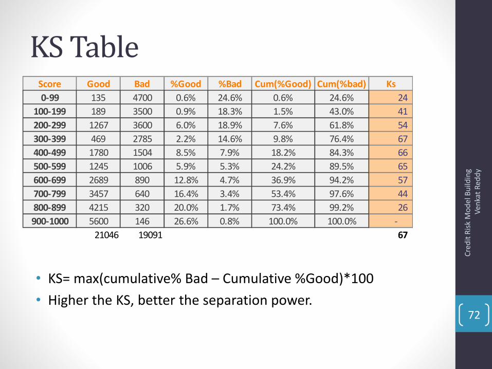
KS Table
• KS= max(cumulative% Bad – Cumulative %Good)*100
• Higher the KS, better the separation power.
Score Good Bad %Good %Bad Cum(%Good) Cum(%bad) Ks
0-99 135 4700 0.6% 24.6% 0.6% 24.6% 24
100-199 189 3500 0.9% 18.3% 1.5% 43.0% 41
200-299 1267 3600 6.0% 18.9% 7.6% 61.8% 54
300-399 469 2785 2.2% 14.6% 9.8% 76.4% 67
400-499 1780 1504 8.5% 7.9% 18.2% 84.3% 66
500-599 1245 1006 5.9% 5.3% 24.2% 89.5% 65
600-699 2689 890 12.8% 4.7% 36.9% 94.2% 57
700-799 3457 640 16.4% 3.4% 53.4% 97.6% 44
800-899 4215 320 20.0% 1.7% 73.4% 99.2% 26
900-1000 5600 146 26.6% 0.8% 100.0% 100.0% -
21046 19091 67
Cre
dit
Ris
k M
od
el B
uild
ing
Ven
kat
Red
dy
72

Lab: KS Calculation
Score Good Bad
0-99 1135 5700
100-199 1689 4500
200-299 1267 3600
300-399 1469 2785
400-499 1780 1504
500-599 1245 1006
600-699 2689 3913
700-799 3457 4491
800-899 4215 2046
900-1000 5600 1957
24546 31502 Cre
dit
Ris
k M
od
el B
uild
ing
Ven
kat
Red
dy
73

PSI
• We built a model on population A, we want to use it on population B
• Population stability report compare distributions of recent applicants to a standard population distribution(development sample)
• The comparison is done in order to see if there is any shift in in the distribution of new applicants.
• PSI = j [(A - B) * ln (A / B)]
• Where, A = % of observations in group j in development sample, and B = % of observations in group j in validation sample
Cre
dit
Ris
k M
od
el B
uild
ing
Ven
kat
Red
dy
74

PSI Table
• PSI = j [(A - B) * ln (A / B)]
• Higher the PSI, higher the population shift
Score Dev Recent %A %B %A-%B Ln(%A/%B) PSI
0-99 4229 5234 8.6% 10.7% -2.1% -22.1% 0.00
100-199 4360 4557 8.9% 9.3% -0.5% -5.2% 0.00
200-299 6245 4255 12.7% 8.7% 4.0% 37.6% 0.01
300-399 4771 4325 9.7% 8.9% 0.8% 9.1% 0.00
400-499 4747 5789 9.7% 11.9% -2.2% -20.6% 0.00
500-599 4577 6546 9.3% 13.4% -4.1% -36.5% 0.01
600-699 4899 4980 10.0% 10.2% -0.2% -2.4% 0.00
700-799 4337 4421 8.8% 9.1% -0.2% -2.7% 0.00
800-899 4515 4311 9.2% 8.8% 0.3% 3.9% 0.00
900-1000 6500 4399 13.2% 9.0% 4.2% 38.3% 0.02
49180 48817 5.7%
Cre
dit
Ris
k M
od
el B
uild
ing
Ven
kat
Red
dy
75
Lab: PSI calculation
• Download Model Validation data
• Draw rank ordering graph for model-1 and model-2. What is your inference?
• Calculate KS for model-1 and model-2.
• Which one of these two models have higher separation power
• Find the PSI for scorecard-1 & scorecard-2
• Which one can be used for 2013 population?
Cre
dit
Ris
k M
od
el B
uild
ing
Ven
kat
Red
dy
76

Triggers for Model validation
• There is red flag if:
• For ECM, KS<20 and for application/acquisition KS<15 at the time of model validation
• KS drops more than 25% (or more than 10 points in absolute) from development of model to validation
• KS drops more than 15% (or more than 5 points in absolute) from previous validation
• If KS Drop is significant and rank ordering is also not perfect then we go for re development or re estimation of the model
Cre
dit
Ris
k M
od
el B
uild
ing
Ven
kat
Red
dy
77

Model Building stepsObjective
Exclusions
Observation point and/or window
Performance window
Bad definition
Segmentation
Variable selection
Regression Line
Model validation
Model recalibration
Cre
dit
Ris
k M
od
el B
uild
ing
Ven
kat
Red
dy
78

Model recalibration
• Re-estimation or Re-development?
• Decided by using Character analysis
• Find the PSI for each variable in the final model
• If the population remained unchanged with respect to al variables then simply re-estimate the coefficients.
• What if the population changed drastically with respect to a variable?
Income Dev Sample Recent(2013) %A %B %A-%B Ln(%A/%B) CI(Income)
0-1499 4229 3678 9.5% 3.8% 5.7% 91.0% 0.05
1500-4600 5900 7800 13.2% 8.1% 5.1% 49.1% 0.03
4601- 5900 7923 9848 17.8% 10.2% 7.5% 55.3% 0.04
5901-8000 10240 14078 23.0% 14.6% 8.4% 45.2% 0.04
8001-12000 6900 18905 15.5% 19.6% -4.1% -23.7% 0.01
12001-20000 5400 17000 12.1% 17.7% -5.5% -37.6% 0.02
>20001 3981 25000 8.9% 26.0% -17.0% -106.7% 0.18
44573 96309 36.9%
Cre
dit
Ris
k M
od
el B
uild
ing
Ven
kat
Red
dy
79

Lab: Character Analysis
• Find the distribution shift with respect to variable “Number of loans”
• Is the population changed with respect to this variable?
Cre
dit
Ris
k M
od
el B
uild
ing
Ven
kat
Red
dy
80

Thank You
Cre
dit
Ris
k M
od
el B
uild
ing
Ven
kat
Red
dy
81
Credits:• Gopal Prasad Malakar• V2K Vijay• Balakrishna Rajagopal