crime and justice - bocsar issues in crime and justice number 138 december 2009 this bulletin has...

Contemporary Issues in Crime and Justice Number 138

December 2009

This bulletin has been independently peer reviewed.

CRIME AND JUSTICEBulletin NSW Bureau of Crime

Statistics and Research

Prison populations and correctional outlays: The effect of reducing re-imprisonmentDon Weatherburn1, Gary Froyland2, Steve Moffatt3 & Simon Corben4

Between 1998 and 2008, the Australian imprisonment rate (per capita) rose 20 per cent. In 2008, net recurrent and capital expenditure on prisons in Australia exceeded $2.6 billion per annum. Efforts to reduce the prison population through the creation of alternatives to custody have not been very successful. This bulletin explores the potential savings in prison costs and prison numbers of reducing the rate at which prisoners return to custody. The results of our analysis suggest that modest reductions in the rate at which offenders are re-imprisoned would result in substantial savings in prisoner numbers and correctional outlays. A ten per cent reduction in the overall re-imprisonment rates would reduce the prison population by more than 800 inmates, saving $28 million per year. Comparable reductions in the number of new sentenced prisoners also produce benefits but they are smaller. The potential benefits of reducing the rate of re-imprisonment among subgroups of offenders with a high re-imprisonment rate are particularly noteworthy. A 10 per cent reduction in the Indigenous re-imprisonment rate, for example, would reduce the Indigenous sentenced prisoner population by 365 inmates, resulting in savings of more than $10 million per annum.

INTRODUCTION

Between 1998 and 2008, the Australian imprisonment rate (per capita) rose 20 per cent (Australian Bureau of Statistics 2008). Over the same period the Indigenous imprisonment rate rose by 41 per cent. On any given day, more than 27,000 people are now held in Australian prisons (Australian Bureau of Statistics 2008). Currently, it costs more than $200 per day to keep an offender in prison. In 2008, net recurrent and capital expenditure on prisons in Australia exceeded $2.6 billion per annum. National expenditure per person in the population, based on net recurrent expenditure on corrective services, increased in real terms over the last five years, from $100 in 2003-04 to $115 in 2007-08 (SCRGSP 2009, p. 8.4).

Over the last two decades, State and Territory Governments have created a number of front-end alternatives to prison (e.g. suspended sentences, community service orders, home detention) to try and curb the growth in prison numbers and correctional outlays. There is limited evidence that these alternatives to prison have been effective in reducing the use of imprisonment. Most studies find that alternative sanctions tend to be imposed on offenders who would not have gone to prison anyway (Bottoms 1981; Chan & Zdendowski 1986a; 1986b; Tonry & Lynch 1996; Brignell & Poletti (2003); a problem known as net-widening. Brignell and Poletti (2003), for example, found that the introduction of suspended sentences in New South Wales (NSW) resulted in a reduction in the use of fines and probation rather than a reduction in the rate of imprisonment.

Limited Australian research has explored on the potential benefits of back-end strategies (i.e. strategies that reduce the number of offenders who return to custody) in reducing prison numbers and correctional spending. This is unfortunate for three reasons. First, the rate of return to prison is high. In their longitudinal study of re-offending amongst NSW parolees, for example, Jones et al. (2006) found that 64 per cent were reconvicted of a further offence and 41 per cent were re-imprisoned within three years. Second, in NSW (and perhaps other States as well) the number of offenders entering prison on their first custodial sentence is actually lower than the number returning to prison. In fact, the ratio of previously sentenced prisoners to new sentenced prisoners has increased somewhat over the last few years (see Figure 1).

2

B U R E A U O F C R I M E S T A T I S T I C S A N D R E S E A R C H

Third, the available evidence suggests that the benefits arising from increased imprisonment rates have been fairly modest. The growth in NSW imprisonment rates appears to have played some role in reducing overall levels of property crime in Australia between 2000 and 2008 but the dominant factors appear to have been a reduction in heroin use, rising average weekly earnings and falling long-term unemployment (Moffatt, Weatherburn & Donnelly 2005). Most rigorous studies find that higher imprisonment rates are associated with lower crime rates but the relationship appears to be weak. In his

review of the relevant literature, Spelman (2000) found that a 10 per cent increase in the rate of imprisonment in the United States produced, at best, a 2-4 per cent reduction in serious crime.

In 2006, a comprehensive meta-analysis of correctional programs by the Washington State Institute for Public Policy revealed that it is possible to reduce adult recidivism by up to 20 per cent using strategies that cost considerably less than imprisonment (Aos et al. 2006). Table 1 lists some of the programs identified by Aos et al. (2006, p.

9) as having a high net present value. The net present values in the table represent the long-run benefits per offender of crime reduction minus the net up-front costs of the program. Most of the programs in the table can be provided to prisoners either in custody or upon release.

The purpose of this bulletin is to estimate the benefits, in terms of prison numbers and prison costs, of a reduction in the rate at which prisoners return to custody. Since we cannot do this by experiment we use a simple mathematical model to simulate the effect of changing the rate of return to custody. The next section describes the model and its assumptions. The section that follows shows how we estimate the parameters of the model (e.g. the fraction that currently return) and test the model’s validity. The fourth section presents the results of our analysis and the final section discusses the policy significance of our findings. Readers uncomfortable with mathematics might wish to skip to the section labeled ‘Results’.

THE MATHEMATICAL MODEL

ORIGIN OF THE MODEL

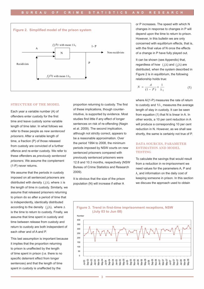
Blumstein and his colleagues (Blumstein & Larson 1969; Blumstein & Larson 1971; Belkin, Blumstein & Glass 1973) were amongst the first (if not the first) to propose that the criminal justice system could be modelled as a feedback system. Their simplest model assumed that the number of people in the criminal justice system at any given time was the sum of those arriving in the system for the first time and those returning to the system after a delay. To calculate the number in the system at any given time, rates of return were assumed to be unrelated to the length of time spent in the system. Here we take a similar approach to modelling the number of people in prison. Our model is depicted in Figure 2.

Figure 1. Ratio of previously sentenced prisoner receptions to new sentenced prisoner receptions, NSW (July 03 to Jun 08)

0.00

0.50

1.00

1.50

2.00

2.50

3.00

Jul-0

3Se

p-03

Nov-0

3Ja

n-04

Mar-0

4Ma

y-04

Jul-0

4Se

p-04

Nov-0

4Ja

n-05

Mar-0

5Ma

y-05

Jul-0

5Se

p-05

Nov-0

5Ja

n-06

Mar-0

6Ma

y-06

Jul-0

6Se

p-06

Nov-0

6Ja

n-07

Mar-0

7Ma

y-07

Jul-0

7Se

p-07

Nov-0

7Ja

n-08

Mar-0

8Ma

y-08

Ratio

Table 1: Net present values for selected correctional programs (Aos et al. 2006, p. 9)

ProgramNet present value

($US)

Vocational education in prison 13,738

Intensive supervision: treatment-oriented programs 11,563

General education in prison (basic education or post-secondary) 10,669

Cognitive-behavioral therapy 10,054

Drug treatment in community 10,299

Correctional industries in prison 9,439

Drug treatment in prison 7,835

Adult drug courts 4,767

Employment and job training in the community 4,359

Sex offender treatment in prison with aftercare 3,258

3


STRUCTURE OF THE MODEL

Each year a variable number (A) of offenders enter custody for the first time and leave custody some variable length of time later. In what follows we refer to these people as new sentenced prisoners. After a variable length of time, a fraction (P) of those released from custody are convicted of a further offence and re-enter custody. We refer to these offenders as previously sentenced prisoners. We assume the complement (1-P) never returns.

We assume that the periods in custody imposed on all sentenced prisoners are distributed with density ƒ1(D), where D is the length of time in custody. Similarly, we assume that released prisoners returning to prison do so after a period of time that is independently, identically distributed according to the density ƒ2(D), where D is the time to return to custody. Finally, we assume that time spent in custody and time between release from custody and return to custody are both independent of each other and of A and P.

This last assumption is important because it implies that the proportion returning to prison is unaffected by the length of time spent in prison (i.e. there is no specific deterrent effect from longer sentences) and that the length of time spent in custody is unaffected by the

proportion returning to custody. The first of these implications, though counter-intuitive, is supported by evidence. Most studies find little if any effect of longer sentences on risk of re-offending (Nagin et al. 2009). The second implication, although not strictly correct, appears to be a reasonable approximation. Over the period 1994 to 2008, the minimum periods imposed by NSW courts on new sentenced prisoners compared with previously sentenced prisoners were 12.8 and 10.3 months, respectively (NSW Bureau of Crime Statistics and Research 2009).

It is obvious that the size of the prison population (N) will increase if either A

Figure 2. Simplified model of the prison system

N A

P

1- P

Non-recidivists

Recidivists

f1(∆)

f2(∆)

with mean 1/λ1

with mean 1/λ2

or P increases. The speed with which N changes in response to changes in P will depend upon the time to return to prison. However, in this bulletin we are only concerned with equilibrium effects, that is, with the final value of N once the effects of a change in P have fully played out.

It can be shown (see Appendix) that, regardless of how ƒ1(D) and ƒ2(D) are distributed, when the system described in Figure 2 is in equilibrium, the following relationship holds true:

where A/(1-P) measures the rate of return to custody and 1/λ1 measures the average length of stay in custody. It can be seen from equation (1) that N is linear in A. In other words, a 10 per cent reduction in A will produce a corresponding 10 per cent reduction in N. However, as we shall see shortly, the same is certainly not true of P.

DATA SOURCES, PARAMETER ESTIMATION AND MODEL TESTING

To calculate the savings that would result from a reduction in re-imprisonment we need values for the parameters A, P and λ1 and information on the daily cost of keeping someone in prison. In this section we discuss the approach used to obtain

1

1)1( λ×

−=

PAN (1)

Figure 3. Trend in first-time imprisonment receptions, NSW (July 03 to Jun 08)

0

50

100

150

200

250

300

350

400

Jul-0

3Se

p-03

Nov-0

3Ja

n-04

Mar-0

4Ma

y-04

Jul-0

4Se

p-04

Nov-0

4Ja

n-05

Mar-0

5Ma

y-05

Jul-0

5Se

p-05

Nov-0

5Ja

n-06

Mar-0

6Ma

y-06

Jul-0

6Se

p-06

Nov-0

6Ja

n-07

Mar-0

7Ma

y-07

Jul-0

7Se

p-07

Nov-0

7Ja

n-08

Mar-0

8Ma

y-08

Number

4


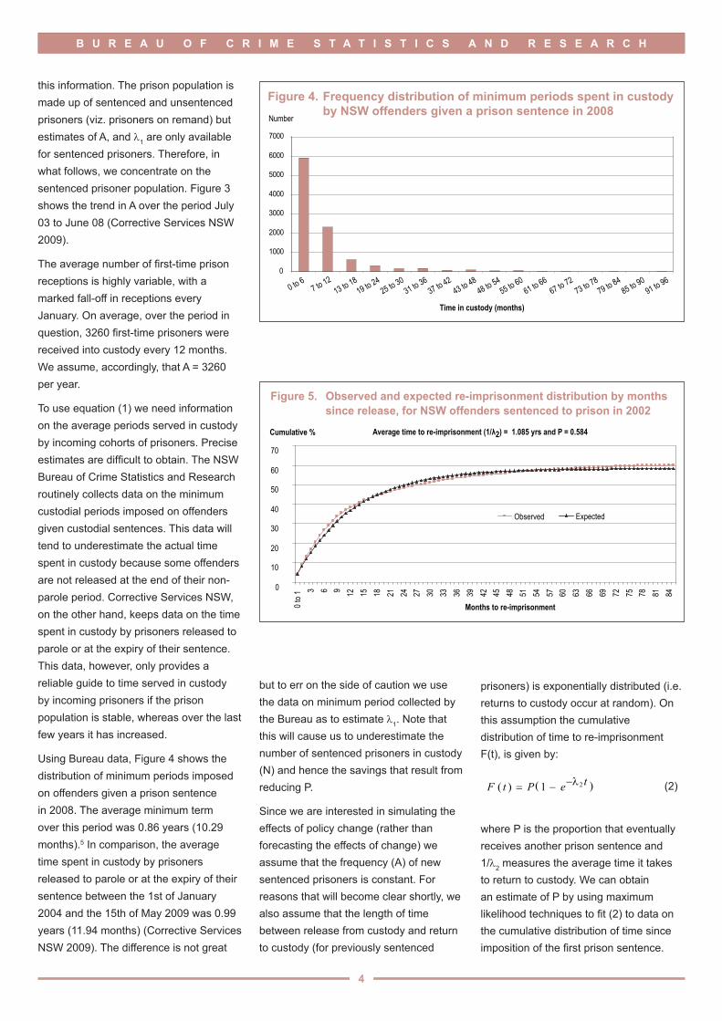
this information. The prison population is made up of sentenced and unsentenced prisoners (viz. prisoners on remand) but estimates of A, and λ1 are only available for sentenced prisoners. Therefore, in what follows, we concentrate on the sentenced prisoner population. Figure 3 shows the trend in A over the period July 03 to June 08 (Corrective Services NSW 2009).

The average number of first-time prison receptions is highly variable, with a marked fall-off in receptions every January. On average, over the period in question, 3260 first-time prisoners were received into custody every 12 months. We assume, accordingly, that A = 3260 per year.

To use equation (1) we need information on the average periods served in custody by incoming cohorts of prisoners. Precise estimates are difficult to obtain. The NSW Bureau of Crime Statistics and Research routinely collects data on the minimum custodial periods imposed on offenders given custodial sentences. This data will tend to underestimate the actual time spent in custody because some offenders are not released at the end of their non-parole period. Corrective Services NSW, on the other hand, keeps data on the time spent in custody by prisoners released to parole or at the expiry of their sentence. This data, however, only provides a reliable guide to time served in custody by incoming prisoners if the prison population is stable, whereas over the last few years it has increased.

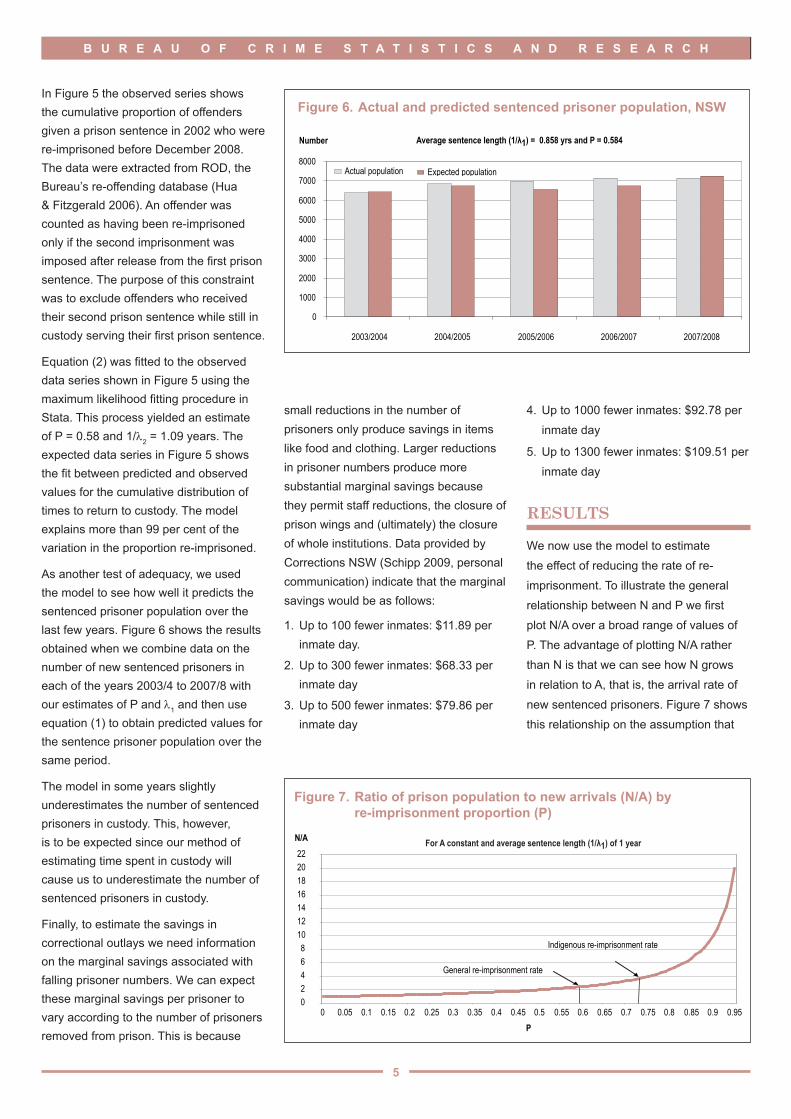
Using Bureau data, Figure 4 shows the distribution of minimum periods imposed on offenders given a prison sentence in 2008. The average minimum term over this period was 0.86 years (10.29 months).5 In comparison, the average time spent in custody by prisoners released to parole or at the expiry of their sentence between the 1st of January 2004 and the 15th of May 2009 was 0.99 years (11.94 months) (Corrective Services NSW 2009). The difference is not great

Figure 4. Frequency distribution of minimum periods spent in custody by NSW offenders given a prison sentence in 2008

0

1000

2000

3000

4000

5000

6000

7000

0 to 67 to 12

13 to 1819 to 24

25 to 3031 to 36

37 to 4243 to 48

48 to 5455 to 60

61 to 6667 to 72

73 to 7879 to 84

85 to 9091 to 96

Time in custody (months)

Number

Figure 5. Observed and expected re-imprisonment distribution by months since release, for NSW offenders sentenced to prison in 2002 Cumulative %

Months to re-imprisonment

0

10

20

30

40

50

60

70

0 to 1

3 6 9 12 15 18 21 24 27 30 33 36 39 42 45 48 51 54 57 60 63 66 69 72 75 78 81 84

Observed Expected

Average time to re-imprisonment (1/λ2) = 1.085 yrs and P = 0.584

but to err on the side of caution we use the data on minimum period collected by the Bureau as to estimate λ1. Note that this will cause us to underestimate the number of sentenced prisoners in custody (N) and hence the savings that result from reducing P.

Since we are interested in simulating the effects of policy change (rather than forecasting the effects of change) we assume that the frequency (A) of new sentenced prisoners is constant. For reasons that will become clear shortly, we also assume that the length of time between release from custody and return to custody (for previously sentenced

prisoners) is exponentially distributed (i.e. returns to custody occur at random). On this assumption the cumulative distribution of time to re-imprisonment F(t), is given by:

where P is the proportion that eventually receives another prison sentence and 1/λ2 measures the average time it takes to return to custody. We can obtain an estimate of P by using maximum likelihood techniques to fit (2) to data on the cumulative distribution of time since imposition of the first prison sentence.

(2)( )tePtF 21)( −λ−=

5


In Figure 5 the observed series shows the cumulative proportion of offenders given a prison sentence in 2002 who were re-imprisoned before December 2008. The data were extracted from ROD, the Bureau’s re-offending database (Hua & Fitzgerald 2006). An offender was counted as having been re-imprisoned only if the second imprisonment was imposed after release from the first prison sentence. The purpose of this constraint was to exclude offenders who received their second prison sentence while still in custody serving their first prison sentence.

Equation (2) was fitted to the observed data series shown in Figure 5 using the maximum likelihood fitting procedure in Stata. This process yielded an estimate of P = 0.58 and 1/λ2 = 1.09 years. The expected data series in Figure 5 shows the fit between predicted and observed values for the cumulative distribution of times to return to custody. The model explains more than 99 per cent of the variation in the proportion re-imprisoned.

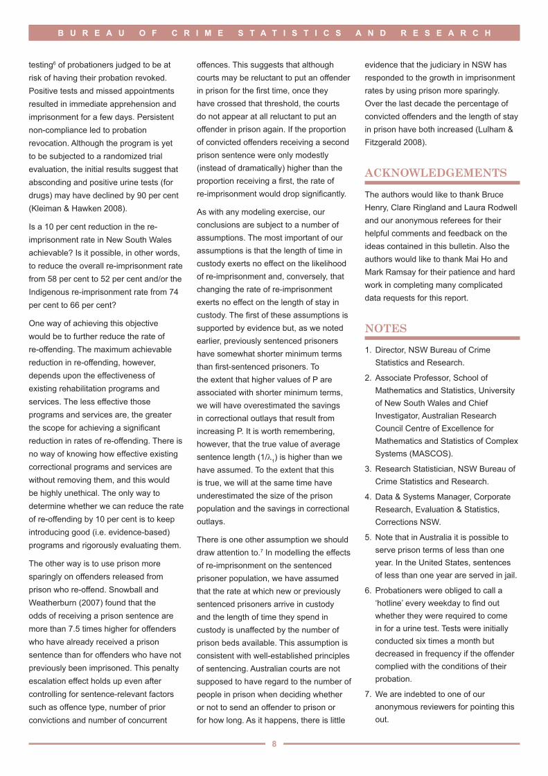
As another test of adequacy, we used the model to see how well it predicts the sentenced prisoner population over the last few years. Figure 6 shows the results obtained when we combine data on the number of new sentenced prisoners in each of the years 2003/4 to 2007/8 with our estimates of P and λ1 and then use equation (1) to obtain predicted values for the sentence prisoner population over the same period.

The model in some years slightly underestimates the number of sentenced prisoners in custody. This, however, is to be expected since our method of estimating time spent in custody will cause us to underestimate the number of sentenced prisoners in custody.

Finally, to estimate the savings in correctional outlays we need information on the marginal savings associated with falling prisoner numbers. We can expect these marginal savings per prisoner to vary according to the number of prisoners removed from prison. This is because

small reductions in the number of prisoners only produce savings in items like food and clothing. Larger reductions in prisoner numbers produce more substantial marginal savings because they permit staff reductions, the closure of prison wings and (ultimately) the closure of whole institutions. Data provided by Corrections NSW (Schipp 2009, personal communication) indicate that the marginal savings would be as follows:

1. Up to 100 fewer inmates: $11.89 per inmate day.

2. Up to 300 fewer inmates: $68.33 per inmate day


Figure 6. Actual and predicted sentenced prisoner population, NSW

0

1000

2000

3000

4000

5000

6000

7000

8000

2003/2004 2004/2005 2005/2006 2006/2007 2007/2008

Number

Actual population Expected population

Average sentence length (1/λ1) = 0.858 yrs and P = 0.584



RESULTS

We now use the model to estimate the effect of reducing the rate of re-imprisonment. To illustrate the general relationship between N and P we first plot N/A over a broad range of values of P. The advantage of plotting N/A rather than N is that we can see how N grows in relation to A, that is, the arrival rate of new sentenced prisoners. Figure 7 shows this relationship on the assumption that

Figure 7. Ratio of prison population to new arrivals (N/A) by re-imprisonment proportion (P)

0

1000

2000

3000

4000

5000

6000

7000

8000

2003/2004 2004/2005 2005/2006 2006/2007 2007/2008

N/A

Actual popPredicted

02468

10121416182022

0 0.05 0.1 0.15 0.2 0.25 0.3 0.35 0.4 0.45 0.5 0.55 0.6 0.65 0.7 0.75 0.8 0.85 0.9 0.95P

General re-imprisonment rate

Indigenous re-imprisonment rate

For A constant and average sentence length (1/λ1) of 1 year

6


A = 3260. For convenience we assume average sentence length (1/λ1) of one year.

As the figure shows, the relationship is highly non-linear. At P = 0, the sentenced prisoner population is equal to the arrival rate of new sentenced prisoners (viz. 3260). When P = 0.50 (i.e. half of all released prisoners return to custody), the prison population is double the number of new sentenced prisoners arriving every year. At P = 0.75, the prison population is four times larger than the number of new sentenced prisoners arriving every year. At P = 0.95, the prison population is 20 times larger than the number of new sentenced prisoners every year. It is obvious that there are substantial benefits to be had from reducing the rate of re-imprisonment among any group of offenders with a high rate of re-imprisonment.

The first three columns of Table 2 provide an estimate of the savings in prisoner numbers and correctional expenditure that result from reducing P by 1, 5, 10, 15 and 20 per cent of its current estimated value (0.58), assuming A remains constant at 3260 and average sentence length (1/λ1) = 0.86 years. The maximum (20 per cent) has been chosen on the basis that this was the maximum reduction in re-offending observed in the meta-analysis of correctional programs carried out by Aos et al. (2006). Columns 4, 5 and 6 show the effect of comparable reductions in the number of new sentenced prisoners, assuming P remains constant at its current estimated value. The cost savings have been calculated on the basis of (1) to (5) above.

Reducing P consistently produces bigger reductions in the sentenced prisoner population (and larger savings) than reducing A. A ten per cent reduction in P (which would involve reducing P from 58 per cent to 52 per cent), for example, would reduce the sentenced prisoner population by an estimated 829 inmates, producing annual savings in excess of

$28 million in recurrent expenditure. A 10 per cent reduction in A, on the other hand, would reduce the sentenced prisoner population by 673 inmates, producing annual savings around $23 million. Although the effect of changing P and A is not markedly different, there are good reasons for believing that a 10 per cent reduction in P is much easier to produce than a 10 per cent reduction in A. We discuss these reasons later in the bulletin.

The overall benefits in reducing P are similar to those associated with a reduction in A because P lies in a range where its relationship with N is fairly linear. We would expect to find much more substantial effects among offenders that have high rates of return to prison. Figure 8 shows the cumulative proportion of offenders re-imprisoned by Indigenous

status. It can be seen that Indigenous offenders have much higher rates of re-imprisonment than non-Indigenous offenders. In fact when equation (2) is fitted to the cumulative distributions of re-imprisonment shown in Figure 8 (using the same methods as before), the resulting estimates are P(Indigenous) = 0.74, while P(non-Indigenous) = 0.52.

The first three columns of Table 3 provide an estimate of the savings in Indigenous prisoner numbers and correctional expenditure on Indigenous offenders that result from reducing P by 1, 5, 10, 15 and 20 per cent of its current estimated value (0.74) for Indigenous offenders, assuming A remains constant at 610 new sentenced prisoners every year. As with Table 2, columns 4, 5 and 6 show the effect of comparable reductions in the number of

Table 2: Savings in prisoner numbers and correctional spending for previously sentenced (P) prisoners versus new (A)

Reduction in P (%)

Reduction in N

Savings ($mill)

Reduction in A (%)

Reduction in N

Savings ($mill)

1 93 0.40 1 67 0.29

5 442 12.88 5 336 9.80

10 829 28.07 10 673 22.78

15 1171 46.82 15 1009 40.33

20 1476 59.00 20 1345 53.78

Figure 8. Cumulative re-imprisonment distribution by months since release, for NSW offenders sentenced to prison in 2002

0

10

20

30

40

50

60

70

80

0 to 1 3 6 9 12 15 18 21 24 27 30 33 36 39 42 45 48 51 54 57 60 63 66 69 72 75 78 81

Months to re-imprisonment

Cumulative %

ATSI Non ATSI

ATSI: average time to re-imprisonment (1/λ2) = 0.917 yrs and P = 0.737 Non ATSI: average time to re-imprisonment (1/λ2) = 1.208 yrs and P = 0.522

7


new sentenced prisoners. The estimates in Table 3, it should be noted, are based on the assumption that 1/λ1 = 0.72 years (8.6 months). This is the average minimum period imposed on Indigenous offenders receiving a custodial sentence in 2008 (NSW Bureau of Crime Statistics and Research 2009).

Reducing P(Indigenous) produces substantial benefits. A ten percent reduction, for example, would reduce the Indigenous sentenced prisoner population by an estimated 365 inmates, producing an estimated saving of more than $10 million per annum. A ten per cent reduction in A(Indigenous), on the other hand, would reduce the Indigenous sentenced prisoner population by 166 inmates, producing estimated savings of only about $4 million. A 20 per cent reduction in A(Indigenous) would have less effect on the Indigenous sentenced prisoner population (and corresponding correctional outlays) than a 10 per cent reduction in the rate of re-imprisonment.

DISCUSSION

The purpose of this bulletin was to explore the benefits in terms of prison numbers and costs of a reduction in the rate at which prisoners return to custody. The results of our analysis suggest that modest reductions in the rate at which offenders are re-imprisoned would result in substantial savings in prisoner numbers and correctional

outlays. Comparable reductions in the number of new sentenced prisoners also produce benefits but they are smaller. A ten per cent reduction in the rate of re-imprisonment (which would involve reducing P from 58 per cent to 52 per cent), for example, would reduce the sentenced prisoner population by an estimated 829 inmates, producing annual savings of in excess of about $28 million in recurrent expenditure. A 10 per cent reduction in A, on the other hand, would reduce the sentenced prisoner population by 673 inmates, producing savings of around $23 million.

The potential benefits of reducing the rate of re-imprisonment among Indigenous offenders are particularly noteworthy. A ten percent reduction, for example, would reduce the Indigenous sentenced prisoner population by an estimated 365 inmates, producing an estimated saving of more than $10 million per annum. A ten per cent reduction in the rate at which new Indigenous sentenced prisoners arrive in custody, by contrast, would reduce the Indigenous sentenced prisoner population by only 166 inmates, producing estimated savings of only about $4 million. In fact a 20 per cent reduction in the number of new Indigenous sentenced prisoners would have less effect on the Indigenous sentenced prisoner population (and corresponding correctional outlays) than a 10 per cent reduction in the rate of Indigenous re-imprisonment. This suggests that efforts to reduce the over-

representation of Indigenous offenders in custody might be better off focused on back-end strategies than on front-end strategies.

Indigenous offenders are not the only group that would benefit from reduced rates of re-imprisonment. Substantial benefits in terms of reduced prison numbers and prison costs are to be expected from a reduction in re-imprisonment rates among any subgroup of offenders with a high rate of re-imprisonment. This would include offenders with a prior drug conviction, younger offenders and offenders convicted of assault, robbery and/or property offenders (Jones et al. 2006).

There are a number of other advantages in focusing policy on the rate of re-imprisonment. Governments generally have far less control over the flow of new offenders into prison than they have over the flow of offenders back to prison. Parliament can reduce the number of offenders sent to prison by removing penal sanctions from certain offences. Once enacted, however, penal sanctions are rarely removed, especially from offences that usually result in imprisonment. They can create alternatives to prison in the hope that the courts use prison more sparingly. This strategy, however, has not proved very effective in reducing the number of offenders going to prison. The way Governments deal with offenders while in custody or after release, by contrast, can have a big effect on the rate of return to custody and, therewith, the size of the sentenced prisoner population.

The Hawaii Opportunity Probation with Enforcement (HOPE) program provides a case in point. Five or six years ago, the probation service in Hawaii was burdened with high rates of probation violation. The problem was believed by some to stem from a low perceived risk of apprehension for probation violation. To heighten the perceived risk of apprehension, Hawaii introduced frequent random drug

Table 3: Savings in indigenous prisoner numbers and correctional spending for previously sentenced (P) prisoners versus new (A)

Reduction in P (%)

Reduction in N

Savings ($mill)

Reduction in A (%)

Reduction in N

Savings ($mill)

1 45 0.20 1 17 0.07

5 205 5.11 5 83 0.36

10 365 10.64 10 166 4.15

15 493 14.38 15 250 6.23

20 599 20.27 20 333 9.70

8


testing6 of probationers judged to be at risk of having their probation revoked. Positive tests and missed appointments resulted in immediate apprehension and imprisonment for a few days. Persistent non-compliance led to probation revocation. Although the program is yet to be subjected to a randomized trial evaluation, the initial results suggest that absconding and positive urine tests (for drugs) may have declined by 90 per cent (Kleiman & Hawken 2008).

Is a 10 per cent reduction in the re-imprisonment rate in New South Wales achievable? Is it possible, in other words, to reduce the overall re-imprisonment rate from 58 per cent to 52 per cent and/or the Indigenous re-imprisonment rate from 74 per cent to 66 per cent?

One way of achieving this objective would be to further reduce the rate of re-offending. The maximum achievable reduction in re-offending, however, depends upon the effectiveness of existing rehabilitation programs and services. The less effective those programs and services are, the greater the scope for achieving a significant reduction in rates of re-offending. There is no way of knowing how effective existing correctional programs and services are without removing them, and this would be highly unethical. The only way to determine whether we can reduce the rate of re-offending by 10 per cent is to keep introducing good (i.e. evidence-based) programs and rigorously evaluating them.

The other way is to use prison more sparingly on offenders released from prison who re-offend. Snowball and Weatherburn (2007) found that the odds of receiving a prison sentence are more than 7.5 times higher for offenders who have already received a prison sentence than for offenders who have not previously been imprisoned. This penalty escalation effect holds up even after controlling for sentence-relevant factors such as offence type, number of prior convictions and number of concurrent

offences. This suggests that although courts may be reluctant to put an offender in prison for the first time, once they have crossed that threshold, the courts do not appear at all reluctant to put an offender in prison again. If the proportion of convicted offenders receiving a second prison sentence were only modestly (instead of dramatically) higher than the proportion receiving a first, the rate of re-imprisonment would drop significantly.

As with any modeling exercise, our conclusions are subject to a number of assumptions. The most important of our assumptions is that the length of time in custody exerts no effect on the likelihood of re-imprisonment and, conversely, that changing the rate of re-imprisonment exerts no effect on the length of stay in custody. The first of these assumptions is supported by evidence but, as we noted earlier, previously sentenced prisoners have somewhat shorter minimum terms than first-sentenced prisoners. To the extent that higher values of P are associated with shorter minimum terms, we will have overestimated the savings in correctional outlays that result from increasing P. It is worth remembering, however, that the true value of average sentence length (1/λ1) is higher than we have assumed. To the extent that this is true, we will at the same time have underestimated the size of the prison population and the savings in correctional outlays.

There is one other assumption we should draw attention to.7 In modelling the effects of re-imprisonment on the sentenced prisoner population, we have assumed that the rate at which new or previously sentenced prisoners arrive in custody and the length of time they spend in custody is unaffected by the number of prison beds available. This assumption is consistent with well-established principles of sentencing. Australian courts are not supposed to have regard to the number of people in prison when deciding whether or not to send an offender to prison or for how long. As it happens, there is little

evidence that the judiciary in NSW has responded to the growth in imprisonment rates by using prison more sparingly. Over the last decade the percentage of convicted offenders and the length of stay in prison have both increased (Lulham & Fitzgerald 2008).

ACKNOWLEDGEMENTS

The authors would like to thank Bruce Henry, Clare Ringland and Laura Rodwell and our anonymous referees for their helpful comments and feedback on the ideas contained in this bulletin. Also the authors would like to thank Mai Ho and Mark Ramsay for their patience and hard work in completing many complicated data requests for this report.

NOTES

1. Director, NSW Bureau of Crime Statistics and Research.

2. Associate Professor, School of Mathematics and Statistics, University of New South Wales and Chief Investigator, Australian Research Council Centre of Excellence for Mathematics and Statistics of Complex Systems (MASCOS).

3. Research Statistician, NSW Bureau of Crime Statistics and Research.

4. Data & Systems Manager, Corporate Research, Evaluation & Statistics, Corrections NSW.

5. Note that in Australia it is possible to serve prison terms of less than one year. In the United States, sentences of less than one year are served in jail.

6. Probationers were obliged to call a ‘hotline’ every weekday to find out whether they were required to come in for a urine test. Tests were initially conducted six times a month but decreased in frequency if the offender complied with the conditions of their probation.

7. We are indebted to one of our anonymous reviewers for pointing this out.

9


REFERENCES

Aos, S., Miller, M., & Drake, E. 2006, Evidence-Based Public Policy Options to Reduce Future Prison Construction, Criminal Justice Costs, and Crime Rates. Olympia: Washington, State Institute for Public Policy.

Australian Bureau of Statistics 2008, Prisoners in Australia, Australian Bureau of Statistics 2008, Catalogue no. 4517.0, Canberra.

Belkin, J., Blumstein, A. & Glass, W. 1973, ‘Recidivism as feedback process: An analytical model and empirical validation’, Journal of Criminal Justice, vol. 1, pp. 7-26.

Blumstein, A., Larson, R. 1969, ‘Models of a Total Criminal Justice System’, Operational Research, vol. 17, pp. 199-232.

Blumstein, A., Larson, R. 1971, ‘Problems in Modeling and Measuring Recidivism’, Journal of Research in Crime and Delinquency, 8: pp. 124-132.

Bottoms, A. 1981, ‘Suspended Sentence in England: 1967-1978’, British Journal of Criminology, vol. 21: pp. 1-26.

Brignell, G. and Poletti, P. 2003, Suspended Sentences in New South Wales, Sentencing Trends and Issues no. 29. Sydney: Judicial Commission of New South Wales.

Chan, J. & Zdenkowski, G. 1986a, ‘Just Alternatives—Part 1’, Australian and New Zealand Journal of Criminology, vol. 19, pp. 67-90.

Chan, J. & Zdenkowski, G. 1986b, ‘Just Alternatives—Part 11’, Australian and New Zealand Journal of Criminology, vol. 19, pp. 131-154.

Corrective Services NSW 2009, Unpublished data.

Hua, J. & Fitzgerald, J. 2006, Matching Court Records to Measure Re-offending, Crime and Justice Bulletin 95, NSW Bureau of Crime Statistics and Research, Sydney.

Jones, C., Hua, J., Donnelly, N., McHutchinson, J. & Heggie, K. 2006, Risk of re-offending amongst parolees, Crime and Justice Bulletin 91, NSW Bureau of Crime Statistics and Research, Sydney.

Kleiman, M.A. & Hawkin, A. 2008, Fixing the Parole System, Issues in Science and Technology, Summer, 2008. http://www.spa.ucla.edu/faculty/kleiman/fixing%20th/20Parole%20System%20-%20Issues.pdf. Extracted 2nd November, 2009.

Lulham, R. & Fitzgerald, J. 2008, Trends in bail and sentencing outcomes in New South Wales Criminal Courts: 1993-2007, Crime and Justice Bulletin 124, NSW Bureau of Crime Statistics and Research, Sydney.

Moffatt, S., Weatherburn, D. & Donnelly, N. 2005, What caused the drop in property crime? Crime and Justice Bulletin 85, NSW Bureau of Crime Statistics and Research, Sydney.

Nagin, D., Cullen, F., and Jonson, C. 2009 (forthcoming), ‘Imprisonment and Reoffending.’ In M. Tonry, ed., Crime and Justice: An Annual Review of Research (vol. 38). Chicago: University of Chicago Press.

NSW Bureau of Crime Statistics and Research 2009, Unpublished data.

Schipp,.G. 2009, Deputy Commissioner, NSW Department of Corrective Services, personal communication.

SCRGSP (Steering Committee for the Review of Government Service Provision) 2009, Report on Government Services 2009, Productivity Commission, Canberra.

Spelman, W. 2000, What recent studies do (and don’t) tell us about imprisonment and crime, in Crime and Justice: A Review of Research vol. 27, M. Tonry, (ed). University of Chicago Press, Chicago, pp. 419-494.

Snowball, L. & Weatherburn 2007, Does Racial Bias in Sentencing Contribute to Indigenous Over-representation in Prison? Australian and New Zealand Journal of Criminology, vol. 40(3), pp. 272-290.

Tonry, M. & Lynch, M. 1996, ‘Intermediate Sanctions’, Michael Tonry (Ed). (1996). Crime and Justice: A Review of Research, vol. 20. Chicago, IL: University of Chicago Press. pp. 99-144.

10


(2)L : = N * ⌡⌠0

∞ Q (∆ ) /∆ d ∆ .

APPENDIX

We assume that incoming prisoners have their prison terms independently, identically distributed (IID) according to the density ƒ1(D), where 0≤D≤∞ is the term length. Similarly, we assume that released prisoners returning to prison do so after a period of time that is IID according to the density ƒ2(D), where 0≤D≤∞ is the time to return.

We note that if the prison system has been initialised by IID prison terms then the terms of the total prison population (as distinct from incoming prisoners) are distributed as ƒ1(D) · D. Let:

be the density of prisoners in custody as a function of term length.

We assume that the rate at which new incoming prisoners enter is A. A fraction, P, of outgoing prisoners are eventually re-sentenced and return after a time distributed according to ƒ2.

Suppose that we are at equilibrium and let the number of prisoners in custody be N*. At equilibrium, the rate of prisoners leaving is:

This is because there are N* Q (D) d D prisoners with terms in [D,D+dD] and their rate of leaving is (N* Q (D) d D) / D .

The rate of prisoners entering is A+PL. Note that the time taken for prisoners to return to prison, as described by ƒ2 , has no effect on this entry rate because we are at equilibrium.

At steady state, A+PL = L, so A-(1-P)L = 0 and L = A/(1-P). Thus by (2),

Note that

where ƒ1 is the average incoming term length.

⌡⌠0

∞ Q (∆ )/∆ d ∆ =

⌡⌠0

∞ f1 (∆ ) d∆

⌡⌠0

∞ f1 (∆ ). ∆ d ∆

= 1

f *1

,

In particular, if f1(∆ ) = λ1e−λ1∆ N * = A

(1−P ) λ1. f *1 = 1/λ1, then and

Thus N*= A f *

1(1−P ) .

(1)Q ( ∆)= f1

(∆ ) . ∆

⌡⌠0

∞ f

1(∆ ) . ∆ d ∆

(3)N*= L

⌡⌠0

∞ Q(∆)/∆ d∆

= A

(1−P)( ⌡⌠0

∞ Q(∆)/∆ d∆)

.

11


Other titles in this seriesNo.137 The impact of restricted alcohol availability on alcohol-related violence in Newcastle, NSW

No.136 The recidivism of offenders given suspended sentences

No.135 Drink driving and recidivism in NSW

No.134 How do methamphetamine users respond to changes in methamphetamine price?

No.133 Policy and program evaluation: recommendations for criminal justice policy analysts and advisors

No.132 The specific deterrent effect of custodial penalties on juvenile re-offending

No.131 The Magistrates Early Referral Into Treatment Program

No.130 Rates of participation in burglary and motor vehicle theft

No.129 Does Forum Sentencing reduce re-offending?

No.128 Recent trends in legal proceedings for breach of bail, juvenile remand and crime

No.127 Is the assault rate in NSW higher now than it was during the 1990s?

No.126 Does receiving an amphetamine charge increase the likelihood of a future violent charge?

No.125 What caused the decrease in sexual assault clear-up rates?

No.124 Trends in bail and sentencing outcomes in New South Wales Criminal Courts: 1993-2007

No.123 The Impact of the high range PCA guideline judgment on sentencing for PCA offences in NSW

No.122 CHERE report: The Costs of NSW Drug Court

No.121 The NSW Drug Court: A re-evaluation of its effectiveness

No.120 Trends in property and illicit drug-related crime in Kings Cross: An update

No.119 Juror understanding of judicial instructions in criminal trials

No.118 Public confidence in the New South Wales criminal justice system

No.117 Monitoring trends in re-offending among offenders released from prison

No.116 Police-recorded assaults on hospital premises in New South Wales: 1996-2006

No.115 Does circle sentencing reduce Aboriginal offending?

No.114 Did the heroin shortage increase amphetamine use?

No.113 The problem of steal from motor vehicle in New South Wales

No.112 Community supervision and rehabilitation: Two studies of offenders on supervised bonds

No.111 Does a lack of alternatives to custody increase the risk of a prison sentence?

No.110 Monitoring trends in re-offending among adult and juvenile offenders given non-custodial sanctions

No.109 Screening juvenile offenders for more detailed assessment and intervention

No.108 The psychosocial needs of NSW court defendants

No.107 The relationship between head injury and violent offending in juvenile detainees

No.106 The deterrent effect of higher fines on recidivism: Driving offences

No.105 Recent trends in property and drug-related crime in Kings Cross

No.104 The economic and social factors underpinning Indigenous contact with the justice system: Results from the 2002 NATSISS survey


NSW Bureau of Crime Statistics and Research - Level 8, St James Centre, 111 Elizabeth Street, Sydney 2000 [email protected] • www.bocsar.nsw.gov.au • Ph: (02) 9231 9190 • Fax: (02) 9231 9187

ISSN 1030 - 1046 • ISBN 978-1-921626-67-8 © State of New South Wales through the Department of Justice & Attorney General 2009. You may copy, distribute, display, download and otherwise freely deal with this work for any purpose, provided that you attribute the Department of Justice & Attorney General as the owner. However, you must obtain permission if you wish to

(a) charge others for access to the work (other than at cost), (b) include the work in advertising or a product for sale, or (c) modify the work.

No.103 Reoffending among young people cautioned by police or who participated in a Youth Justice Conference

No.102 Child sexual assault trials: A survey of juror perceptions

No.101 The relationship between petrol theft and petrol prices

No.100 Malicious Damage to Property Offences in New South Wales

No.99 Indigenous over-representation in prision: The role of offender characteristics

No.98 Firearms and violent crime in New South Wales, 1995-2005

No.97 The relationship between methamphetamine use and violent behaviour

No.96 Generation Y and Crime: A longitudinal study of contact with NSW criminal courts before the age of 21

No.95 Matching Court Records to Measure Reoffending

No.94 Victims of Abduction: Patterns and Case Studies

No.93 How much crime does prison stop? The incapacitation effect of prison on burglary

No.92 The attrition of sexual offences from the New South Wales criminal justice system

No.91 Risk of re-offending among parolees

No.90 Long-term trends in property and violent crime in NSW: 1990-2004

No.89 Trends and patterns in domestic violence

No.88 Early-phase predictors of subsequent program compliance and offending among NSW Adult Drug Court participants

No.87 Driving under the influence of cannabis: The problem and potential countermeasures

No.86 The transition from juvenile to adult criminal careers

No.85 What caused the recent drop in property crime?

No.84 The deterrent effect of capital punishment: A review of the research evidence

No.83 Evaluation of the Bail Amendment (Repeat Offenders) Act 2002

No.82 Long-term trends in trial case processing in NSW

No.81 Sentencing drink-drivers: The use of dismissals and conditional discharges

No.80 Public perceptions of crime trends in New South Wales and Western Australia

No.79 The impact of heroin dependence on long-term robbery trends

No.78 Contact with the New South Wales court and prison systems: The influence of age, Indigenous status and gender

No.77 Sentencing high-range PCA drink-drivers in NSW

No.76 The New South Wales Criminal Justice System Simulation Model: Further Developments

No.75 Driving under the influence of cannabis in a New South Wales rural area

No.74 Unemployment duration, schooling and property crime

No.73 The impact of abolishing short prison sentences

No.72 Drug use monitoring of police detainees in New South Wales: The first two years

No.71 What lies behind the growth in fraud?

crime and justice - bocsar issues in crime and justice number 138 december 2009 this bulletin has...

Documents