crimestat iii - icpsr · crimestat iii part iii: spatia l modeling. 8.1 chapter 8 ... (rosenblatt,...
TRANSCRIPT

CrimeStat III
P art III: Sp atia l Mod e ling
8.1
Chapter 8Kernel Density Interpolation
In th is chapt er , we discuss t ools a imed a t int erpola t ing incident s, us ing the ker neldensit y approach . In terpolation is a t echnique for genera lizing incident loca t ion s to anent ir e a rea . Whereas the spa t ia l d is t r ibu t ion and hot spot st a t is t ics provide st a t is t ica lsummar ies for the da ta in ciden t s themselves, in terpola t ion techniques genera lize thoseda ta inciden t s t o the ent ire r egion . In pa r t icu lar , th ey provide density est imates for a llpa r t s of a region (i.e., a t any loca t ion ). The densit y est im ate is an in tensit y var ia ble, a Z-value, th a t is est ima ted a t a pa r t icu lar loca t ion . Consequ ent ly, it can be displayed byeith er sur face maps or cont our ma ps th at show the intensity at all locat ions.
There a re many in terpola t ion techniques, such as Kr igin g, t r end sur faces, loca lregression models (e.g., Loess, sp lines), and Dir ich let t essella t ions (Anselin, 1992;Clevelan d, Grosse a nd Sh yu, 1993; Venables an d Ripley, 1997). Most of these r equire avar iable t ha t is bein g est imated as a fun ction of loca t ion. H owever , kernel densityestim ation is an in terpola t ion technique tha t is appropr ia te for in dividua l poin t loca t ion s(Silverm an, 1986; Härdle, 1991; Bailey an d Ga t rell, 1995; Bur t an d Barber, 1996; Bowmanand Azalini, 1997).
Kernel Dens i ty Est imat ion
Ker nel densit y est imat ion involves p lacing a sym met r ical sur face over each poin t ,eva lua t ing the d is tance from the poin t to a reference loca t ion based on a mathemat ica lfunct ion , and summing the va lue of a ll the su r faces for tha t r eference loca t ion . Th ispr ocedure is r epea ted for a ll referen ce locat ions. I t is a t echn ique t ha t wa s developed inthe la te 1950s as a n a lt er na t ive m et hod for est imat ing the den sit y of a h ist ogra m(Rosenbla t t , 1956; Wh it t le, 1958; Parzen , 1962). A h is togr am is a gr aphic r epresen ta t ion ofa frequency dis t r ibu t ion . A cont in uous va r ia ble is divided in to in terva ls of size, s (theint erval or bin widt h), an d t he number of cases in each int erval (bin) ar e counted a nddispla yed a s block diagrams. Th e h ist ogram is a ssumed to rep resen t a sm ooth , under lyingdis t r ibu t ion (a densit y fu nct ion ). H owever , in order to est im ate a smooth densit y fu nct ionfrom the h istogra m, tr adit iona lly resea rchers h ave link ed a djacent var iable int ervals byconnect ing the m idpoint s of th e in ter va ls with a ser ies of lines (Figu re 8.1).
Unfor tuna tely, doing th is causes t h ree s t a t ist ical problems (Bowman and Azalini,1997):
1. Inform at ion is discar ded becau se all cases with in an int erval ar e assigned tothe midpoin t . The wider the in terva l, the gr ea ter the in format ion loss.
2. The technique of connect in g t he midpoin t s leads to a discont in uous and notsm ooth densit y function even though the under lying den sit y function isassu med t o be sm ooth . To compen sa te for th is, resea rchers will r edu ce thewidth of the in ter val. Thus, t he den sit y function becomes sm oother wit h

Constructing A Density Estimate From A HistogramMethod of Connecting Midpoints
Variable Classification Interval (bin)
Freq
uenc
y
12
34
56
7
50
40
30
20
10
0
Figure 8.1:

8.3
sm aller int erval widths, alt hough st ill not very sm ooth . Fu r ther , th ere arelimits t o th is t echnique a s t he sa mple size decreases wh en the bin widt h getssm aller, even tua lly becoming too sm all to pr odu ce reliable est ima tes.
3. The t echn ique is depen dent on a n arbit ra r ily defined in ter val size (binwidth). By makin g th e int erval wider , th e est ima tor becomes cru der and,conversely, by makin g th e int erval nar rower , th e est ima tor becomes finer .However , t he under lyin g densit y d is t r ibu t ion is assumed to be smooth andcon t inuous and not dependen t on the in t erva l s ize of a h is togram.
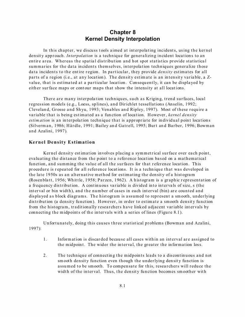
To handle th is pr oblem, Rosen blat t (1956), Whitt le (1958) and P arzen (1962)developed the kernel densit y m ethod in order to avoid the fir st two of these difficult ies; thebin wid th issue st ill r emain s. What they did was to pla ce a smooth kernel function , r a therthan a block, over ea ch point and sum the functions for ea ch locat ion on the scale . Figure8.2 illu st ra tes the process with five point loca t ions . As seen , over ea ch locat ion, asym met r ical ker nel fun ction is p laced; by symmet r ical is mea nt tha t is fa lls off withdis tance from ea ch poin t a t an equ a l ra te in both dir ections a roun d each poin t . In th iscase, it is a normal dist r ibut ion , but other types of symmet r ica l dist r ibut ion have beenused. The under lying den sity distr ibut ion is est ima ted by summing the individua l ker nelfunct ions a t all loca t ions to p roduce a smooth cumula t ive dens ity funct ion . Not ice tha t thefun ctions a re sum med at every point a long the scale and n ot just a t t he point locat ions. The adva ntages of th is a re tha t , fir st , each poin t cont r ibu tes equa lly t o the densit y sur faceand, second, th e resu ltin g dens ity funct ion is con t inu ous a t a ll poin t s a long th e scale.
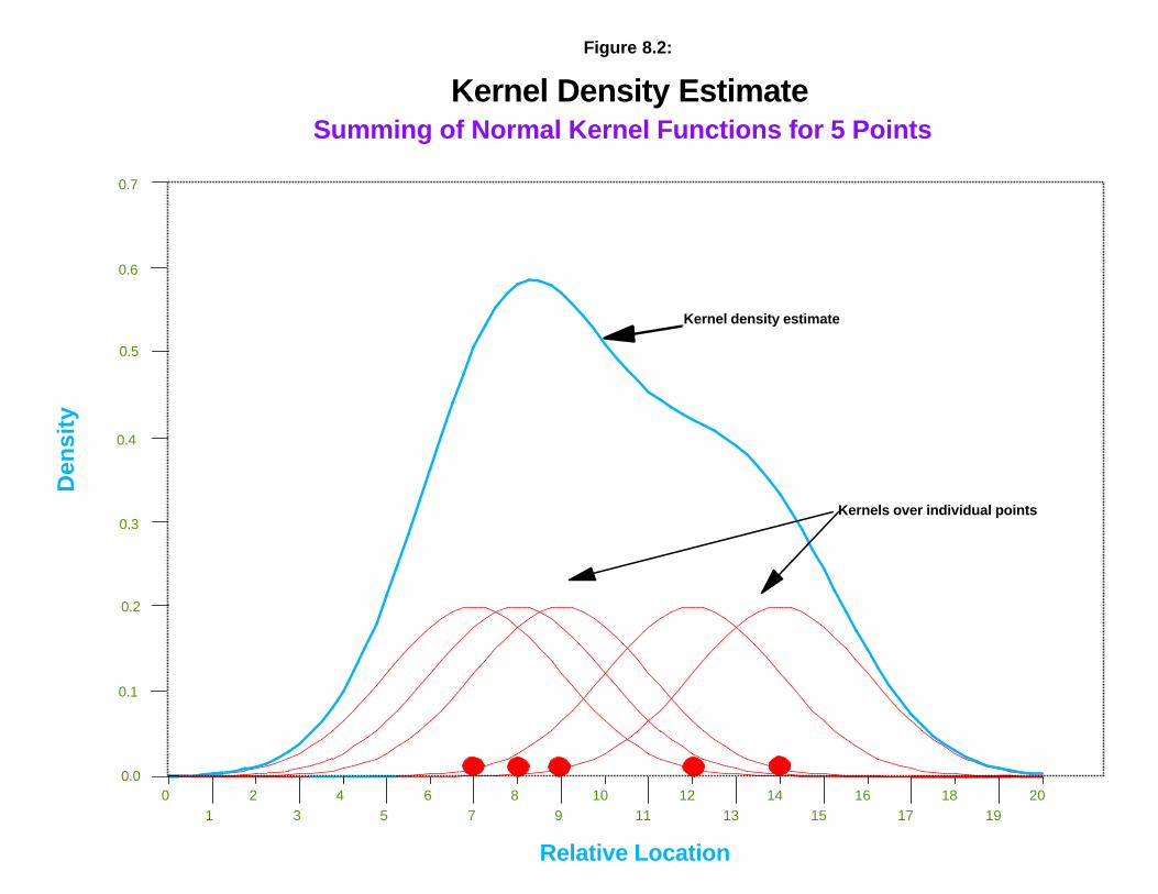
The th ir d problem ment ion ed above, in terva l s ize, s t ill r emain s sin ce the wid th ofth e kernel fun ction can be var ied. In th e kernel density literat ur e, th is is called band wid thand refer s essen t ia lly t o the wid th of the kernel. Figure 8.3 shows a kernel wit h a nar rowbandwidt h placed over the sa me five poin t s wh ile figure 8.4 shows a ker nel with a widerba ndwidt h pla ced over t he poin t s. Clea r ly, th e smoothness of the r esu lt ing den sit yfun ction is a consequence of th e ban dwidth size.
There a re a number of differen t kernel fu nct ion s tha t have been used, a side fromthe norm al dis t r ibu t ion , su ch a s a t r iangular fun ction (Bur t and Ba rber , 1996) or a quar t icfunct ion (Ba iley and Ga t rell, 1995). Figur e 8.5 illus t ra tes a quar t ic funct ion . But thenorm al is t he m ost commonly u sed (Kelsa ll and Diggle, 1995a ).
The n or m a l d ist r ib u ti on funct ion has the followin g fu nct ion a l for m:
d ij2
1 - [--------- ]g(x j) = E{ [Wi * I i] * ----------- * e 2*h 2 } (8.1)
h 2 * 2B
where d ij is the dis t ance between an in ciden t loca t ion and any r eference poin t in the region ,h is t he s t anda rd devia t ion of th e n orm al dis t r ibu t ion (the ba ndwidt h), Wi is a weigh t a tth e point locat ion a nd I i is an int ensity at the poin t loca t ion . This funct ion exten ds t oinfinit y in a ll dir ect ions and, t hus, will be a pp lied to an y loca t ion in the r egion.
Kernel Density EstimateSumming of Normal Kernel Functions for 5 Points
Relative Location
Den
sity
01
23
45
67
89
1011
1213
1415
1617
1819
20
0.7
0.6
0.5
0.4
0.3
0.2
0.1
0.0
Kernel density estimate
Kernels over individual points
Figure 8.2:
Kernel Density EstimateSmaller Bandwidth
Relative Location
Den
sity
01
23
45
67
89
1011
1213
1415
1617
1819
20
1.0
0.9
0.8
0.7
0.6
0.5
0.4
0.3
0.2
0.1
0.0
Kernel density estimate
Figure 8.3:

Relative Location
Den
sity
01
23
45
67
89
1011
1213
1415
1617
1819
20
0.5
0.4
0.3
0.2
0.1
0.0
Kernel density estimate
Kernels over individual points
Kernel Density EstimateLarger Bandwidth
Figure 8.4:

Summing of Quartic Kernel Function
Relative Location
Den
sity
01
23
45
67
89
1011
1213
1415
1617
1819
20
0.18
0.16
0.14
0.12
0.10
0.08
0.06
0.04
0.02
0
Kernel density estimate
Quartic functions over individual points
Kernel Density EstimateFigure 8.5:

8.8
In Crim eS tat, t here a re four a lt erna t ive kernel funct ions tha t can be used , a ll ofwhich have a circumscribed r adius (un like the normal dist r ibut ion). The qua r t i c funct ionis applied to a limit ed area a round ea ch in ciden t poin t defin ed by the radiu s, h . It fa lls offgradu a lly with dis t ance un t il the r adiu s is rea ched . It s functiona l form is:
1. Ou tside t he specified radiu s, h :
g(x j) = 0 (8.2)
2. With in the specified radiu s, h :
3 d ij2
g(x j) = E{ [Wi * I i] * [ ----------] * [1 - -------] 2 } (8.3) h 2 * B h2
where d ij is the dis t ance between an in ciden t loca t ion and any r eference poin t in the region ,h is t he r adiu s of th e sea rch a rea (th e ba ndwidt h), Wi is a weight a t the poin t loca t ion andI i is a n in ten sit y a t the point loca t ion.
The t r ia n gu la r (or conica l) dist r ibut ion fa lls off evenly with dist ance, in a linearrela t ion sh ip . Compared to the quar t ic fu nct ion , it fa lls off more rapid ly. I t a lso has acircum scribed r adius a nd is, th erefore, app lied to a limit ed a rea a round ea ch inciden tpoint, h. Its fun ctiona l form is:
1. Ou tside t he specified radiu s, h :
g(x j) = 0 (8.4)
2. With in the specified radiu s, h :
g(x j) = E [K - K/h ] * d ij (8.5)
where K is a cons tan t . In Crim eS tat, th e const an t K is init ially set t o 0.25 and t hen re-scaled t o ensu re tha t eith er the densit ies or pr obabilit ies su m to their a ppr opr iat e values(i.e., N for densit ies and 1.00 for proba bilit ies).
The nega t i ve exponen t ia l (or peaked) dist r ibu t ion falls off ver y rapid ly withdis tance up to th e circumscr ibed radiu s. I t s functiona l form is:
1. Ou tside t he specified radiu s, h :
g(x j) = 0 (8.6)
2. With in the specified radiu s, h :
g(x j) = E A*e -K*dij(8.7)

8.9
where A is a const an t a nd K is an exponen t. In Crim eS tat’s im plementa t ion , K is set to 3while A is in it ia lly set to 1 a nd then re-sca led to ensure tha t eit her the densit ies orprobabilit ies sum to their appropr ia te va lu es (i.e., N for densit ies and 1.00 forproba bilit ies).
F ina lly, th e u n i for m distribut ion weight s all points with in th e circle equally. Itsfun ctiona l form is:
1. Ou tside t he specified radiu s, h :
g(x j) = 0 (8.8)
2. With in the specified radiu s, h :
g(x j) = EK (8.9)
where K is a const an t . Init ially, K is set to 0.1 but then re-scaled t o ensu re tha t eith er thedensit ies or probabilit ies sum to their appropr ia te va lu es (i.e., N for densit ies and 1.00 forproba bilit ies).
Kern e l P ara m e te rs
The user can select these five differen t ker nel funct ions t o int erpola te the da ta tothe gr id cells. They produce subt le differences in the shape of the in terpola ted sur face orcon tour . The norma l d is t ribu t ion weighs a ll poin t s in t he s tudy a rea , t hough nea r poin t sa re weighted m ore h igh ly than dist an t poin t s. The oth er four techniques use acircumscr ibed circle ar oun d t he gr id cell. The un iform dis t r ibu t ion weigh s a ll point s with inthe circle equa lly. The quar t ic funct ion weighs near poin t s m ore than fa r poin t s, but thefa ll off is gradua l. The t r iangu la r funct ion weighs near poin t s more than fa r poin t s with inthe circle, but the fa ll off is more rapid. Fina lly, th e negat ive exponent ial weighs n earpoin t much m ore h ighly than far poin t s with in the circle.
The use of any of one of these depends on h ow much the user wants t o weigh nearpoint s r ela t ive to fa r point s. Usin g a ker nel fun ction wh ich h as a big differ en ce in t heweight s of near versus far poin t s (e.g., th e negat ive exponent ial or the t r ian gula r ) t ends t opr oduce finer var ia t ions with in the sur face than fun ctions which a re weight more even ly(e.g., t he norma l d is t ribu t ion , t he qua r t ic, or t he un iform); t hese la t t er ones tend to sm ooththe dist r ibut ion more.
S h a p e a n d s iz e of t h e b a n d w i d t h
However , Silverman (1986) has a rgu ed tha t it does not make tha t much differenceas long as t he ker nel is sym met r ica l. Ther e are a lso edge effect s t ha t can occur and t herehave been differen t proposed solu t ion s to th is problem (Ven ables and Ripley, 1997).

8.10
There have a lso been va r ia t ion s of the size of the of ba ndwid th wit h va r iou sformulas a nd cr it er ia (Silver man, 1986; Härdle, 1991; Ven ables and Ripley, 1997). Gen er a lly, bandwidt h choice fall in to eith er fixed or ada pt ive (var iable) choices (Kelsa ll andDiggle, 1995a ; Bailey a nd Gat rell, 1995). Crim eS tat follows t h is dist inction , which will beexpla ined below.
Anoth er suggestion is to use th e Mora n corr elogra m, which was discussed inchapt er 4, to estim ate the sh ape of the weight ing funct ion (Cliff and H agget t , 1988; Baileyand Ga t t rell, 1995). This would be appr opr iat e for var iables t ha t have weights , such aspopu la t ion or em ploymen t . The Moran cor relogra m displa ys t he degree of spa t ia lau tocorrela t ion as a funct ion of dis t ance. Whether the au tocorrela t ion fa lls off qu ick ly ormore slowly can be u sed t o select an approxima te ker nel function (e.g., a n ega t iveexponent ial funct ion fa lls off quickly wher eas a qua r t ic funct ion fa lls off very slowly). Thebandwidth could a lso be selected by the dis t ance a t which the Moran correlogr am levels off(i.e., approaches the global I value). This would lead t o an est imate t ha t minimizes spa t ia lau tocor relat ion in t he da ta set . It would be good for capt ur ing major t r ends in the da ta ,bu t would not be good for iden t ifyin g loca l cluster s (hot spots) sin ce the bandwid th dis t ancewould incorpora te most of a met ropolita n a rea .
Three-d im ensiona l kerne l s
The ker nel funct ion can be expan ded t o more than two dimensions (Hä rdle, 1991;Ba iley a nd Gat rell, 1995; Bu r t and Barber , 1996; Bowman and Azalin i, 1997). Figure 8.6sh ows a th ree-dim en siona l norm al dis t r ibu t ion pla ced over each of five point s with theresu lt ing den sit y su r face bein g a su m of a ll five individua l su r faces. Th us, t he m et hod ispa r t icu lar ly appr opr iat e for geogra ph ica l da ta , such a s crime inciden t loca t ions. Themet hod has a lso been developed to rela te t wo or more var iables together by app lying aker nel est ima te to each var iable in t u rn and t hen dividing one by th e other to pr odu ce athree-dim ension a l est im ate of risk (Kelsa ll and Diggle, 1995a ; Bowman and Aza lin i, 1997).
Significance test ing of density est ima tes is m ore complica ted. Cur ren t t echniquestend to focus on simu lat ing sur faces under spa t ially ra ndom as su mpt ions (Bowman an dAza line, 1997; Kelsa ll and Diggle, 1995b). Because of the st ill exper im enta l n a ture of thetes t ing, Crim eS tat does not in clu de any t est in g of densit y est im ates in th is version .
C r i m eS t a t Kerne l Dens i ty Methods
Crim eS tat has t wo int er pola t ion techn iques, both based on the ker nel densit ytechn ique. The firs t app lies t o a s ingle var iable, wh ile the second t o th e r ela t ionsh ipbetween two var iables. Both rout ines h ave a number of opt ions. Figur e 8.7 shows t hein ter pola t ion pa ge in Crim eS tat. User s indica te their choices by clickin g on the tab andmen u item s. F or eit her t echn ique, it is n ecessa ry to ha ve a referen ce file, wh ich is usu a llya gr id pla ced over the study r egion (see chapter 3). The reference file represen t s the regionto wh ich the kernel est im ate will be genera lized (figu re 8.8).

+
+
+
+
=
Kernel Density SurfacesSumming of Normal Kernel Surfaces for 5 Points
Figure 8.6:

Interpolation ScreenFigure 8.7:

Miles
420
Figure 8.8:
Grid Cell Structure for Baltimore Region108 Width x 100 Height Grid Cells
Baltimore County
City of Baltimore
D
!
!
Upper-right Coordinate
Lower-left Coordinate

8.14
S in g le D e n si ty Es ti m at e s
The single ker nel densit y rout ine in Crim eS tat is a pp lied t o a dist r ibu t ion of pointloca t ions, such a s cr ime inciden t s. It can be used with either a pr imary file or a seconda ryfile; the pr im ary file is the defau lt . F or exa mple, t he pr im ary file can be the loca t ion ofmotor veh icle t hefts. Th e poin t s can a lso have a weigh t ing or an associa ted in ten sit yva r ia ble (or both). F or exa mple, t he poin t s could represen t the loca t ion of police st a t ion swh ile t he weight s (or in ten sit ies) repr esen t the number of calls for service. Again , the u sermu st be car eful in h aving both a weight ing var iable and a n int ensity var iable as th erout ine will u se both var iables in calcu la t ing densit ies ; th is could lea d t o double weight ing.
Having defined the file on the pr ima ry (or seconda ry) file tabs, th e user indica testhe rou t ine by checkin g th e ‘Single’ box. Also, it is necessa ry to define a reference file,eit her an exist ing file or one gen er a ted by Crim eS tat (see chapt er 3). Ther e are otherpar am eters t ha t m ust be defined.
F ile to be In te rp ola te d
The user must indicate wh et her the pr imary file or t he seconda ry file (if used) is t obe int erpolated.
Method of Interpolat ion
The user must indicate t he m et hod of in ter pola t ion . Five types of ker nel densit yestimat ors a re used:
1. Norm al dis t r ibu t ion (bell; defau lt )2. Uniform (fla t ) dist r ibu t ion3. Quar t ic (spher ica l) d is t r ibu t ion 4. Tr ia ngu la r (conica l) d is t r ibu t ion5. Nega t ive exponent ia l (peaked) dis t r ibu t ion
In our experien ce, th ere are advantages to each . The normal dist r ibut ion pr odu cesan est im ate over the en t ir e region whereas the other four produce est im ates only for thecir cumscr ibed bandwid th r adius. If t he d is t ribu t ion of poin t s is spar se towards the ou terpar t s of the region , t hen the four cir cumscr ibed funct ion s will n ot produce est im ates forthose a reas, whereas the normal will. Con versely, t he normal d is t r ibu t ion can cause someedge effect s t o occur (e.g., spikes a t the edge of the reference grid), pa r t icu lar ly if there aremany point s n ear one of the bounda r ies of the st udy ar ea . The four circum scribedfunct ions will p roduce les s of a problem a t t he edges , a lt hough they s till can produce somespikes . With in the fou r cir cumscr ibed funct ions, t he un iform and qua r t ic t end to smoothth e data more whereas t he tr iangular a nd n egat ive exponent ial tend t o empha size ‘peaks’and ‘va lleys’. The differ en ces between these differ en t ker nel functions a re small, however . Th e u ser sh ould pr obably st a r t wit h the default norm al fun ction and a dju st accord ingly tohow the sur face or cont our looks.

8.15
Choice of Band w idth
The user must in dica te how bandwid ths a re to be defin ed. There a re two types ofba ndwidt h for the s ingle ker nel den sit y rout ine, fixed in ter va l or a da pt ive in ter va l.
Fixed interva l
With a fixed bandwidt h , the u ser must specify the in ter val to be used a nd t he un it sof measu rement (squ ared m iles, squ ared n au t ica l miles, squared feet, squared k ilometers,or squ ared met er s). Depen din g on the t ype of ker nel es t imate u sed, t h is in ter val has as ligh t ly d ifferen t mean ing. For t he norma l kernel funct ion , t he bandwid th is the s tanda rddevia t ion of t he norma l d is t ribu t ion . For t he un iform, qua r t ic, t r iangu la r , or nega t iveexponent ia l ker nels , the ba ndwidt h is t he r adiu s of th e sea rch a rea to be in ter pola ted.
Ther e a re few guidelines for choosin g a pa r t icula r bandwidt h oth er than by visu a linspection (Venables an d Ripley, 1997). Some have ar gued t ha t the ban dwidt h be no lar gerthan the fin est resolu t ion tha t is desir ed and others have argu ed for a va r ia t ion on randomnearest neighbor dist ances (see Spencer Cha iney applica t ion lat er in t h is chapt er ). Oth ershave a rgued for pa r t icula r sizes (Silverman, 1986; Härdle, 1991; Ka da far , 1996; Farewell,1999; Talbot , Kulldor ff, Fora nd, an d H aley, 2000).1 There does not seem t o be consensu son t h is is su e. Consequ en t ly, Crim eS tat leaves t he defin ition up t o the user .
Typica lly, a n ar rower bandwidt h in ter val will lead t o a finer mesh densit y est imatewit h a ll the lit t le peaks a nd va lleys. A lar ger bandwidt h in ter val, on the oth er hand, willlead t o a smoother dis t r ibu t ion and, t her efore, less va r iability bet ween area s. Wh ilesmaller bandwid ths show gr ea ter differen t ia t ion among a reas (e.g., between ‘hot spot ’ and‘low spot ’ zon es), one has to keep in min d the st a t is t ica l precis ion of the es t im ate. If thesa mple size is not ver y large, then a sm aller bandwidt h will lead t o more impr ecision in theest ima tes; the peak s and valleys m ay be noth ing more t han ra ndom var iat ion . On theoth er hand, if the sample size is la rge, t hen a finer densit y est imate can be produced. Ingener a l, it is a good idea to exper imen t wit h differ en t fixed in ter vals t o see wh ich r esu lt smake t he most sen se.
Adapt ive interva l
An adapt ive bandwid th adjust s t he bandwid th in t erva l so tha t a min imum numberof poin t s a r e found. Th is has the advan tage of p rovid ing const an t precis ion of t he es t ima teover the en t ire region . Thus , in a reas tha t have a h igh concen t ra t ion of poin t s , thebandwidt h is na r row whereas in a reas wh ere the concent ra t ion of poin t s is m ore spa rse,the ba ndwidt h will be la rger . This is the defau lt bandwidt h choice in Crim eS tat since webelieve t ha t consis t en cy in st a t ist ical precision is pa ramoun t . The degree of pr ecision isgener a lly depen dent on t he sample size of the ba ndwidt h in ter val. The defau lt is aminimum of 100 poin t s with in the ba ndwidt h radiu s. Th e u ser can make t he es t imatemore fine gra ined by choosing a sm aller number of poin t s (e.g., 25) or more sm ooth bychoosin g a la rger number of poin t s (e.g., 200). Aga in , exper im enta t ion is necessa ry t o seewhich resu lts make t he most sen se.

8.16
Output U nits
The user must indicate t he m ea su rem en t un it s for the den sit y est imate in point sper squ ared m iles, squ ared n au t ica l miles, squared feet, squared k ilometers, or squ aredmeters. The defau lt is point s per squ are mile.
Int e n si ty or We ig h tin g Vari ab le s
If an int ensit y or weight ing var iable is used , th ese boxes must be checked. Becar eful about usin g both an in ten sit y and a weigh t ing var iable t o avoid ‘double weigh t ing’.
D e n s it y Ca lc u la ti on s
The user must indica te the type of ou tpu t for the density est ima tes. Ther e are th reetypes of ca lcu lat ion tha t can be condu cted with the ker nel dens ity rou t ine. Thecalcula t ions a re app lied t o each referen ce cell:
1. The kernel estima tes can be calculat ed as absolute density es t imates usingformulas 8.1-8.9, depen ding on what type of ker nel funct ion is used. Theest ima tes a t each reference cell a re re-scaled so th a t the su m of the densit iesover a ll r eference gr ids equa ls the tota l number of inciden t s ; th is is thedefau lt va lue.
2. The kernel estima tes can be calculat ed as relative density estimat es. Thesedivide t he a bsolut e den sit ies by t he a rea of the gr id cell. I t has t he a dva ntageof in terpret in g t he densit y in terms tha t a re familia r . Thus, instead of adensit y est imate r epresen ted by point s per gr id cell, the r ela t ive densit y willconver t th is t o point s per , sa y, square m ile.
3. The densit ies can be conver ted in to probabilities by dividin g the den sit y a tany one cell by the t ota l number of inciden t s.
Sin ce th e t h ree t ypes of calcula t ion are directly inter rela ted, the out pu t su r face willnot differ in it s var iability. The choice would depen d on whether the ca lcu lat ions a re usedto est im ate absolu te densit ies, r ela t ive densit ies, or probabilit ies. F or compar isonsbet ween differ en t types of crim e or bet ween the same t ype of cr ime and d iffer en t t imeper iods, usu a lly absolut e den sit ies a re t he u n it of choice (i.e., inciden t s per gr id cell). However, t o expres s t he ou tpu t as a pr obability, tha t is, th e likelihood t ha t an inciden twould occur at an y one locat ion, then out put ing th e results as pr obabilities would ma kemore sen se. For d isplay pur poses, however , it makes no difference as both look t he sa me.
Ou tp u t F ile s
Fin a lly, the resu lts can be displayed in an ou tpu t t able or can be ou tpu t int o twoforma t s: 1) Rast er gr id forma t s for display in a su r face mapp ing p rogram- S urfer forWindows ‘.da t ’ format (Golden Software, 1994) or ArcView S pat ial Analyst ‘a sc’ format

8.17
(ESRI, 1998); or 2) Polygon gr ids in ArcView ‘.sh p’, MapIn fo ‘.m if’ or Atlas*GIS ‘.bna ’form at s.2 However , a ll bu t S urfer for Windows r equire t ha t the reference grid be crea tedby Crim eS tat.
Exam ple 1: Kern el De ns ity Estim ate o f Stree t Robberie s
An example can illu st r a t e t he use of t he s ingle kernel density rou t ine. F igu re 8.9shows a S urfer for Windows outpu t of the 1180 st reet robber ies for 1996 in Ba lt im oreCounty. The r efer en ce grid was gener a ted by Crim eS tat and h ad 100 colum ns a nd 108rows. Thus, t he rout ine calcula ted the dist ance between each of the 10,800 r eferen ce cellsand t he 1180 robbery inciden t loca t ions, evalua ted t he ker nel funct ion for each measu reddist ance, an d su mmed t he resu lts for each reference cell. The n ormal dist r ibut ion ker nelfunct ion was selected for the kernel es t imator and an adap t ive bandwid th with a min imumsam ple size of 100 was chosen as t he par am eters.
Th ere a re th ree views in the figu re: 1) a map view showin g t he loca t ion of theinciden t s; 2) a su r face view sh owing a th ree-dimen siona l in ter pola t ion of robbery densit y;and 3) a contour view showin g con tours of high robbery densit y. Th e sur face and contourviews pr ovide differ en t perspect ives . The sur face shows t he pea ks very clear ly and t herela t ive densit y of t he peaks. As can be seen , t he peak for robber ies on the eastern par t ofthe Cou nty is much h igher than the two peaks in the cen t ra l a nd western par t s of theCou nty. Th e contour view can show where these peaks a re loca ted; it is difficult to iden t ifylocat ion clear ly from a th ree-dimensiona l sur face map. Highways an d str eets could beoverla id on top of the contour view to ident ify more pr ecisely where these pea ks a reloca ted.
F igure 8.10 shows an ArcViewS pat ial Analyst map of the r obbery den sit y with therobbery inciden t locat ions over la id on top of th e densit y cont our s. H er e, we can see qu iteclea r ly tha t t here a re th ree s trong concen t r a t ions of inciden t s, one spreading over adis tance of sever a l miles on the west side, one on nort her n border bet ween Ba lt imore Cityand Ba lt imore Coun ty, and one on t he ea st side; th er e is a lso one smaller peak in thesou thea st corner of the County.
From a st a t ist ica l perspective, th e ker nel est ima te is a bet t er ‘hot spot’ ident ifierthan the clus ter ana lysis r ou t ines discussed in cha pt er 6. Clus ter rou t ines group in cident sin to clu ster s and dis t in gu ish between in ciden t s which belon g t o the clu ster and thosewhich do not belong. Depending on which mathemat ica l algor ith ms a re used, differen tclus ter ing rou t ines will retu rn differ ing a lloca t ions of inciden t s t o clus ter s. The k ernelest ima te, on the other hand, is a cont inu ous su r face; the densit ies a re ca lcu lat ed a t allloca t ions; t hus, t he user can visua lly in spect t he va r iabilit y in density and decide wha t t oca ll a ‘hot spot ’ withou t having to define a rbit ra r ily where to cu t -off the ‘hot spot ’ zone.
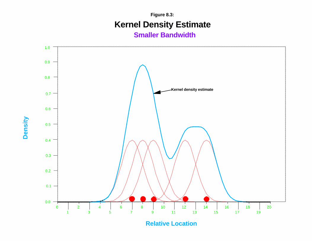
Going back t o the S urfer for Windows outpu t , figu re 8.11 shows the effect s ofvarying the ba ndwidt h pa ramet er s. Ther e a re t h ree fixed ba ndwidt h in ter va ls (0.5, 1, and2 miles respectively) and t here are two ada pt ive ban dwidt h int ervals (a m inim um of 25and 100 poin t s r espectively). As can be seen , th e finen ess of the int erpola t ion is affected by

Baltimore County Robberies: 1996-97Kernel Density Interpolation
Figure 8.9:
Surface View Contour View
Ground Level View
N
-76.80 -76.70 -76.60 -76.50 -76.40 -76.30
39.20
39.30
39.40
39.50
39.60
39.70

Baltimore County
City of Baltimore
Robbery DensityLow
High
Baltimore CountyCity of BaltimoreMajor RoadBaltimore Beltway
0 10 20 Miles
N
EW
S
Figure 8.10Baltimore County Street Robberies: 1996
Kernel Density Estimate
Fixed/ h=0.5 mi Fixed/ h=1.0 mi
Fixed/ h=2.0 mi
Adaptive/ n=50 Adaptive/ n=100
Interpolation of Baltimore County Auto Thefts: 1996Different Smoothing Parameters
Figure 8.11:

Kernel Density Interpolation to Estimate Sampling Bias in the Climatic Response of Sphagnum Spores in North America
Mike Sawada
Laboratory for Applied Geomatics and GIS Science University of Ottawa, Department of Geography, Canada Sphagnum moss, the dominant species of bogs, thrives under certain ranges of temperature and precipitation. Sphagnum releases spores for reproduction and these are transported, often long distances, by wind and water. Thus, the presence of a spore in the fossil record may not indicate nearby Sphagnum plants. However, spores should be most numerous near Sphagnum plants. Over time, these spores and pollen from other plants accumulate in lake and bog sediments and leave a fossil record of vegetation history.
We wanted to use the amount of fossil Sphagnum spores in different parts of North America to infer past climates. To do so, we had to first show that Sphagnum spores are most abundant in climates where Sphagnum plants thrive and secondly, that this center of abundance is not biased sampling because of under sampling in parts of climate space. First, we developed a Sphagnum spore response surface showing the relative abundance of spores along the axes of temperature and precipitation (Fig. A). CrimeStat was used in the second stage to develop a kernel density surface using a quartic kernel for 3007 sample sites within climate space (Fig. B). These were smoothed and visualized in Surfer. The surface showed that the intensity of points is higher in regions surrounding the response maximum. This gave us confidence that the Sphagnum response was real since other parts of climate space are well sampled but unlikely to produce high spore proportions. This fact allowed climate inferences to be made within the fossil record for past time periods using the amount of Sphagnum spores present.
Figures modified from Gajewski, Viau, Sawada et al. 2001. Global Biogeochemical Cycles,

Describing Crime Spatial Patterns By Time of Day
Renato Assunção, Cláudio Beato, Bráulio Silva CRISP, Universidade Federal de Minas Gerais, Brazil
We used the kernel density estimate to visualize time trends for crime
occurrences on a typical weekday. We found markedly different spatial distributions depending on the time, with the amount of crime varying and the hot spots, identified by the ellipses, appearing in different places.
The analysis used 1114 weekday robberies from 1995 to 2000 in downtown
Belo Horizonte. Breaking the data into hours, we used the normal kernel, a fixed bandwidth of 450 meters and outputted densities option (points per square unit of area). Note that the latter option could be useful if one is interested only in the hot spot locations, and not in the distribution during the day. To make the ellipses, we used the nearest neighbor hierarchical spatial clustering technique with a minimum of 35 incidents. We output the results to MapInfo, keeping the same scale for all maps. Four of them are shown below.
9:00 AM 1:00 PM
7:00 PM 11:00 PM

Using Kernel Density Smoothing and Linking to ArcView: Examples from London, England
Spencer Chainey
Jill Dando Institute of Crime Science University College London, England
CrimeStat offers an effective method for creating kernel density surfaces. The
example below uses residential burglary incidents in the London Borough of Croydon, England for the period June 1999 – May 2000 (N=3104). The single kernel routine was used to produce a kernel density surface representing the distribution of residential burglary.
The kernel function used was the quartic, which is favoured by most crime
mappers as it applies added weight to crimes closer to the centre of the bandwidth. Rather than choosing an arbitary interval it is useful to use the mean nearest neighbour distance for different orders of K, which can be calculated by CrimeStat as part of a nearest neighbour analysis. For the Croydon data, an interval of 269 metres was chosen, which relates to a mean nearest neighbour distance at a K-order of 13. The output units were densities in square kilometres and was output to ArcView.
Kernel density estimation is a particularly useful method as it helps to precisely identify the location, spatial extent and intensity of crime hotspots. It is also visually attractive, so helping to invoke further enquiry and the reasoning behind why crime and disorder is concentrated. The density surface that is created can reflect the distribution of incidents against the natural geography of the area of interest, including representing the natural boundaries, such as reservoirs and lakes, or an alignment that follows a particular street in which there is a high concentration of offending. The method is also less subjective if clear guidelines are followed for the setting of parameters.

Infant Death Rate and Low Birth Weight in the I-5 Corridor of Seattle and King County
Richard Hoskins
Washington State Department of Health Olympia, Washington
Although the infant death rate (< 1 year old) has been steadily declining in Washington, the incidence of low birth weight (< 2500 gms) is increasing. This is a significant public health problem, resulting in suffering and high medical cost. If we know where the rates are high at a neighborhood level we can develop more efficient and effective programs. The goal is to determine regions where rates are clustered and to characterize those regions with respect to SES variables from the US Census. Birth and infant death data were geocoded to the street level. In order to detect clusters of high infant death and low birth weight, several CrimeStat tools were used. We find that using several tools at once helps detect regions where something untoward is going on and also helps develops guesses about where other problems might be expected develop.
The result of a kernel density interpolation using a normal estimator is shown above along with an empirical Bayes rate and standardized mortality ratio (SMR) calculated in SAS and mapped in Maptitude (www.caliper.com). Starting with over 2,500 infant deaths, about 25,000 low weight births (out of over 500,000 live births) occurred in the Seattle I-5 corridor region in King County from 1989-2002. The kernel density method was used to detect high rate regions. A clearly articulated region and ridge appears on the grid of the kernel density map and the 3D and prism maps.
I-5 corridor in Kernel density Top: 3-D map: empirical Bayes rate King County interpolation Bottom: Prism map: SMR

8.25
the ban dwidt h choice. For t he th ree fixed int ervals, an int erval of 0.5 miles pr odu ces afiner mesh in terpola t ion than an in terva l of 2 miles , which t ends to ‘oversmooth’ thedist r ibut ion . Per haps, t he int ermedia te int erval of 1 mile gives the best ba lan ce betweenfinen ess a nd gener a lity. For the two ada pt ive int ervals, the minim um sa mple size of 25gives some very specific peak locat ions wher ea s t he ada pt ive in ter val with a minimumsa mple size of 100 gives a sm oother dis t r ibu t ion.
Which of these sh ould be used a s t he best choice would depend on how muchconfidence the ana lys t has in the resu lt s . A key ques t ion is whether the ‘peaks’ a re rea l ormerely byproduct s of sm all sa mple sizes. The best choice would be to produ ce anin terpola t ion tha t fit s the exper ience of the depar tment and officer s who t ravel an a rea .Again , exper imen ta t ion and d iscuss ions with bea t officer s will be necessary to est ablishwhich ban dwidth choice should be used in fut ur e int erpolations.
Note in a ll five of the in terpola t ion s, t here is some bia s a t the edges wit h the City ofBa lt imore (the th ree-s ided a rea in the cen t ra l sou thern par t of the map). S ince thepr ima ry file on ly included incident s for the County, the int erpola t ion nevert heless h asest ima ted some likelihood a t the edges; these a re edge biases and need to be ignored orr emoved with an ASCII ed itor .3 Fur ther , the wider the in ter val chosen , the m ore bias ispr oduced a t the edge.
D u a l Ke rn e l E st im a te s
The dua l ker nel densit y rout ine in Crim eS tat is applied to two d is t r ibu t ions of poin tloca t ions. For example, th e pr ima ry file could be th e loca t ion of au to theft s wh ile theseconda ry file could be th e cen t roids of censu s t r act s, with the popula t ion of the censu st ract being an in ten sit y var iable. Th e dua l rout ine m ust be u sed with both a pr imary fileand a seconda ry file. Also, it is necessa ry to define a referen ce file, either an exist ing fileor one gen er a ted by Crim eS tat (see chapt er 3). Severa l parameters n eed t o be defined .
F ile to be In te rp ola te d
The user m ust indicat e the order of th e int erpolation. The routine uses thelanguage first file and second file in m akin g th e compa r ison (e.g., dividing th e firs t file bythe second; add ing the firs t file t o th e second). The u ser must indicate wh ich is the firs tfile, the pr ima ry or the seconda ry. The defau lt is t ha t the pr ima ry file is the firs t file.
Method of Interpolat ion
The user must indica te the type of ker nel est ima tor . As with the single ker nelden sity rout ine, five types of ker nel dens ity est ima tors a re used
1. Norm al dis t r ibu t ion (bell; defau lt )2. Uniform (fla t ) dist r ibu t ion3. Quar t ic (spher ica l) d is t r ibu t ion
8.26
4. Tr ia ngu la r (conica l) d is t r ibu t ion5. Nega t ive exponent ia l (peaked) dis t r ibu t ion
In our experien ce, th ere are advantages to each . The normal dist r ibut ion pr odu cesan est im ate over the en t ir e region whereas the other four produce est im ates only for thecir cumscr ibed bandwid th r adius. If t he d is t ribu t ion of poin t s is spar se towards the ou terpar t s of the region , t hen the four cir cumscr ibed funct ion s will n ot produce est im ates forthose a reas, whereas the normal will. Con versely, t he normal d is t r ibu t ion can cause someedge effect s t o occur (e.g., spikes a t the edge of the reference grid), pa r t icu lar ly if there aremany point s n ear one of the bounda r ies of the st udy ar ea . The four circum scribedfunct ions will p roduce les s of a problem a t t he edges , a lt hough they s till can produce somespikes . With in the fou r cir cumscr ibed funct ions, t he un iform and qua r t ic t end to smoothth e data more whereas t he tr iangular a nd n egat ive exponent ial tend t o empha size ‘peaks’and ‘va lleys’. The differ en ces between these differ en t ker nel functions a re small, however . Th e u ser sh ould pr obably st a r t wit h the default norm al fun ction and a dju st accord ingly tohow the sur face or cont our looks.
Choice of Band w idth
The user must defin e the bandwid th parameter . There a re th ree types ofbandwid ths for the sin gle kernel densit y r out in e - fixed in terva l, va r ia ble in terva l, orada pt ive in ter va l.
Fixed interva l
With a fixed bandwidt h , the u ser must specify the in ter val to be used a nd t he un it sof measu rement (squ ared m iles, squ ared n au t ica l miles, squared feet, squared k ilometers,or squ ared met er s). Depen din g on the t ype of ker nel es t imate u sed, t h is in ter val has as ligh t ly d ifferen t mean ing. For t he norma l kernel funct ion , t he bandwid th is the s tanda rddevia t ion of t he norma l d is t ribu t ion . For t he un iform, qua r t ic, t r iangu la r , or nega t iveexponent ia l ker nels , the ba ndwidt h is t he r adiu s of th e sea rch a rea to be in ter pola ted. Sin ce th er e a re t wo files being compared, the fixed in ter val is a pp lied both to th e firs t fileand t he second file.
Variable in terva l
With a var iable in ter va l, ea ch file (the first and t he second) have differ en t in ter va ls. For both , t he un it s of measurements must be specified (squared miles, squared nau t ica lmiles , squared feet , squared kilomet er s, or squared met er s). Th er e is a good r ea son wh y auser might want va r ia ble in terva ls . In compar in g t wo kernel est im ates, t he most commoncompar ison is to d ivide one by the other . However , if the dens ity es t imate for a par t icu la rcell in t he denomina tor appr oaches zero, th en the ra t io will blow up a nd become a veryla rge n umber . Visu a lly, th is will be seen as spik es in the dist r ibu t ion, t he r esu lt , usu a lly,of too few cases . In th is case, the user migh t decide to smooth the denomina tor more thannumera tor in order to reduce t hese spik es. F or example, t he in terva l for the fir st file (thenumer a tor) could be 1 m ile wh er ea s t he in ter val for t he second file (th e den omin a tor) could

8.27
be 3 m iles. E xper imen ta t ion will be n ecessary to see wh et her th is is wa r ran ted. But , inour exper ience, it frequ en t ly happen s when eit her ther e a re t wo few cases or ther e is a nirregular boun dar y to th e region with a nu mber of incidents grouped at one of th e edges.
Adapt ive interva l
An adapt ive bandwid th adjust s t he bandwid th in t erva l so tha t a min imum numberof poin t s (sample s ize) is found . Th is sample s ize is app lied to both the fir s t file and thesecond file. It has t he adva ntage of pr ovidin g cons tan t pr ecision of the ker nel es t imateover the en t ire region . Thus , in a reas tha t have a h igh concen t ra t ion of poin t s , thebandwidt h is na r row whereas in a reas wh ere the concent ra t ion of poin t s is m ore spa rse,the ba ndwidt h will be la rger . This is the defau lt bandwidt h choice in Crim eS tat s inceconsis t en cy in st a t ist ical precision is impor tan t . The degree of pr ecision is gener a llydepen den t on the sa mple size of the ban dwidt h int erval. The defau lt is a minim um of 100poin t s. The u ser can make t he es t imate finer by choosin g a sm aller number of poin t s (e.g.,25) or smoother by choosin g a la rger number of poin t s (e.g., 200).
Us e k er n el b a n d w id th s t h a t p r od u ce st a bl e est im a tes
Note: with a du el ker nel ca lcu lat ion , par t icu lar ly the ra t io of one var iable toanother , be carefu l a bout choosin g a very small bandwid th . This could have the effect ofcrea t in g spik es a t the edges of the study a rea or in low popula t ion densit y a reas. F orexa mple, in low popula t ion densit y a reas, t here will p robably be fewer event s than in morebuilt -up area . F or the denomin a tor of a ra t io est im ate, a n ext remely low va lu e could causethe ra t io to be exaggera ted (a ‘spike’) relat ive to neighbor ing grid cells. Using a la rgerbandwidt h will pr odu ce a more st able average.
Output U nits
The user must indicate t he m ea su rem en t un it s for the den sit y est imate in point sper squ ared m iles, squ ared n au t ica l miles, squared feet, squared k ilometers, or squ aredmet ers.
Int e n si ty or We ig h tin g Vari ab le s
If an int ensity or weight ing var iable is used for eith er the firs t file or the second file,these boxes m ust be checked. Be careful a bout usin g both an in ten sit y and a weigh t ingvar iable t o avoid ‘double weigh t ing’.
D e n s it y Ca lc u la ti on s
The user must indicate t he t ype of densit y ou tpu t . Ther e a re six types of densit yca lcu la t ions tha t can be conducted with the dua l kernel dens ity rou t ine. The ca lcu la t ionsare applied to ea ch refer ence cell:
8.28
1. There is th e ratio of densities, tha t is t he first file divided by t he second file. Th is is the defau lt choice. F or example, if the fir st file is the loca t ion of au tothefts in ciden t s a nd t he second file is t he loca t ion of census t r act cen t roidswith the popula t ion assigned a s a n int ensity var iable, th en ra t io of den sit ieswould divide the kernel est im ate for au to theft s by t he kernel est im ate forpopulat ion a nd would be an estimat e of au to th efts r isk.
2. There is also th e log ratio of densities. Th is is the na tu ra l logar ithm of thedensit y ra t io, tha t is
Log ra t io of densit ies = Ln [ g(xj) / g(yj) ] (8.10)
wh er e g(xj) is the densit y est im ate for the fir st file and g(y j) is t he den sit yest ima te for the second file. For a var iable tha t has a spa t ially skeweddistr ibut ion, such t ha t m ost r eference cells ha ve very low density estima tes,bu t a few have very h igh densit y est im ates, con ver t in g t he ra t io in to a logfun ction will tend t o mu te th e spikes th at occur . This measu re ha s beenused in st udies of risk (Kelsa ll and Diggle, 1995b).
3. There is th e absolu te d ifference in densities, th at is th e first file minus t hesecond file. Th is can be a useful ou tpu t for exa min ing differen t ia l effects. For exam ple, by using th e cen t roids of censu s block gr oups (see exam ple 2below) with the popula t ion of the censu s block group ass igned as a n in ten sit yor weigh t ing var iable, t her e is a sligh t bia s p roduced by t he spa t ia lar ra ngements of th e block groups. The U. S. Censu s Bureau suggests th atcensus un it s (e.g., census t r act s , census block groups ) be d rawn so tha t t hereare approximately equa l popula t ion s in each un it . Thus, block gr oupstowards t he cen ter of the met ropolita n a rea tend t o be sm aller because t hereis a h igher popu la t ion densit y a t those loca t ions. Th us, t he spa t ia la r rangemen t of the block groups will ten d t o produce a k er nel es t imatewhich has a h igher va lu e towards the cen ter in dependent of the actua lpopu la t ion of the block group; th e bia s is very sm all, less than 0.1%, but itdoes exist . A more pr ecise est imate could be produced by subt ractin g theker nel es t imate for the block group cent roids withou t u s ing popula t ion as thein ten sit y var iable from t he ker nel es t imate for the block group cent roids withpopula t ion as t he int ensity var iable. The r esu ltin g ou tpu t could then be rea dback in to Crim eS tat and used as a more precise measure of popula t iondis t r ibu t ion . There a re other uses of the difference funct ion , such assu bt ract ing the est ima te for the popula t ion-a t -r isk from t he inciden tdis t r ibu t ion ra ther than taking the r a t io or by calcula t ing the net cha nge inpopulat ion between t wo censuses.
4. There is th e relative d ifference in densities. Like t he r ela t ive densit y in thesingle-ker nel rout ine (discussed above), th e relat ive difference in den sit iesfirs t st anda rdizes th e densit ies of each file by dividing by th e grid cell ar eaand t hen su bt racts the seconda ry file r ela t ive densit y from t he pr imary file

8.29
rela t ive densit y. This can be u seful in calcula t ing changes bet ween two t imeper iods, for example in ca lcu lat ing a cha nge in rela t ive dens ity between twocensuses or a change in the cr im e densit y between two t im e per iods.
5. There is th e sum of the densities, tha t is, t he den sit y est imate for the firs t fileplu s the densit y est im ate for the second file. Aga in , t h is is applied to eachreferen ce cell a t a t ime. A poss ible u se of the sum opera t ion is t o combinetwo differ en t densit y su r faces, for example the den sit y of robber ies plu s t hedensity of assa ults;
6. F ina lly, th ere is th e relative sum of densities between the pr ima ry file andthe seconda ry file. The r elat ive su m of densit ies firs t st anda rdizes th edensities of each file by dividing by th e grid cell ar ea an d th en subtr acts t heseconda ry file r ela t ive densit y from t he pr imary file r ela t ive densit y. Thiscan be usefu l for iden t ifyin g t he tota l effect s of two dis t r ibu t ion s. F orexample, the tota l impact of robber ies and burgla r ies on an a rea can beest im ated by t akin g t he rela t ive densit y of r obber ies and addin g it to therela t ive densit y of burgla r ies. The resu lt is the combin ed rela t ive densit y ofrobber ies and bu rgla r ies per un it a rea (e.g., robber ies and bu rgla r ies persqu are mile).
Ou tp u t F ile s
Fina lly, th e user must specify th e file formats for the ou tpu t . The r esu lts can beout pu t in th ree forms. F ir st , the r esu lt s a re disp layed in an out pu t t able. Second, t heresu lt s can be outpu t in to two ra st er gr id formats for displa y in a su r face mappingprogram: S urfer for Windows format as a ‘.da t ’ file (Golden Software, 1994) and ArcViewS pat ial Analyst format as a ‘.a sc’ file (ESRI , 1998). Th ird , the resu lt s can be ou tpu t aspolygon gr ids in to ArcView ‘.sh p’, MapIn fo ‘.mif’ an d Atlas*GIS ‘.bna’ format (see footnote1). All bu t S urfer for Windows r equ ire t ha t the r efer en ce grid be crea ted by Crim eS tat.
Ex am ple 2: Kerne l Dens i ty Est imates o f Vehic le Thef t s Re lative to Population
As an example of the use of the dua l kernel dens ity rou t ine, the duel rou t ine isapp lied in both the Cit y of Balt imore a nd t he County of Balt imore t o 14,853 m otor veh icletheft loca t ions for 1996 r ela t ive t o th e 1990 popu la t ion of cen su s block groups. Again , arefer en ce grid of 100 columns by 108 rows was gener a ted by Crim eS tat.
Figur e 8.12 shows the r esulting density estima te as a S urfer for Windows ou tpu t ;aga in , t here is a map view, a sur face view, a nd a contour view. The normal k ernel fu nct ionwas u sed a nd a n ada pt ive ban dwidt h of 100 point s wa s selected. As seen , th ere is a ver yhigh concent ra t ion of au to th eft inciden t s with in the cen t ra l pa r t of the m et ropolitan a rea . Th e contour view suggest five or six pea k area s t ha t a re close to each other .

Baltimore County Vehicle Thefts: 1996Kernel Density Interpolation
Figure 8.12:
Surface View Contour View
Ground Level View
N
-76.80 -76.70 -76.60 -76.50 -76.40 -76.30
39.20
39.30
39.40
39.50
39.60
39.70

8.31
Mu ch of th is concent ra t ion , however , is produced by h igh popu la t ion densit y in themet ropolita n cen ter . Figur e 8.13, for exam ple, shows the ker nel est ima te for 1349 censu sblock gr oups for both the City of Balt imore a nd t he County of Balt imore wit h the 1990popula t ion assigned a s t he int ensity var iable. Again , th e normal ker nel funct ion was u sedwit h an adapt ive ba ndwidth of 100 poin t s bein g selected. The map shows th ree views: 1) asu r face view; 2) a contour view; and 3) a groun d level view lookin g directly nort h . Thedist r ibut ion of popula t ion is, of course, also highly concent ra ted in t he met ropolita n cen terwith two pea ks , quite close t o each other with severa l smaller pea ks .
When these t wo kernel es t imates a re compa red usin g the dua l ker nel densit yrou t ine, a more complica ted pictu re emerges (figure 8.14). This r ou t ine h as condu ctedthree oper a t ions: 1) it ca lcula ted the dist ance between each of the 10,800 r eferen ce cellsand t he 14,853 au to theft loca t ions, evalua ted t he ker nel funct ion for each measu reddis tance, a nd summed the resu lt s for each reference cell; 2) it ca lcu la ted the dis t ancebet ween each of the 10,800 r eferen ce cells a nd t he 1349 censu s block groups withpopula t ion a s a n in ten sit y var iable, eva lua ted the ker nel function for ea ch in ten sit y-weight ed dist ance, an d su mmed t he resu lts for each reference cell; and 3) divided t hekernel densit y est im ate for au to theft s by t he kernel densit y est im ate for popula t ion forea ch r efer en ce cell loca t ion.
While the concent ra t ion of motor veh icle t hefts r ela t ive to popu la t ion (‘motor veh icletheft r isk”) is st ill h igh in t he met ropolita n cen ter , th ere are ban ds of h igh r isk t ha t spr eadoutward , pa r t icu la r ly a long major a r t er ia ls . There a re now many ‘hot spot ’ a reas whichhave a h igh dis t r ibu t ion of motor veh icle t hefts r ela t ive to th e r esiden t ia l popu la t ion . Wecould, of course, refine t h is ana lysis fur ther by ta kin g, for exam ple, employment as aba seline va r iable r a ther than popu la t ion ; employmen t is a bet t er indicator for the dayt imepopula t ion dis t r ibu t ion whereas the residen t ia l popula t ion is a bet t er in dica tor forn igh t t im e popula t ion dis t r ibu t ion (Levine, Kim , a nd Nit z, 1995a ; 1995b).
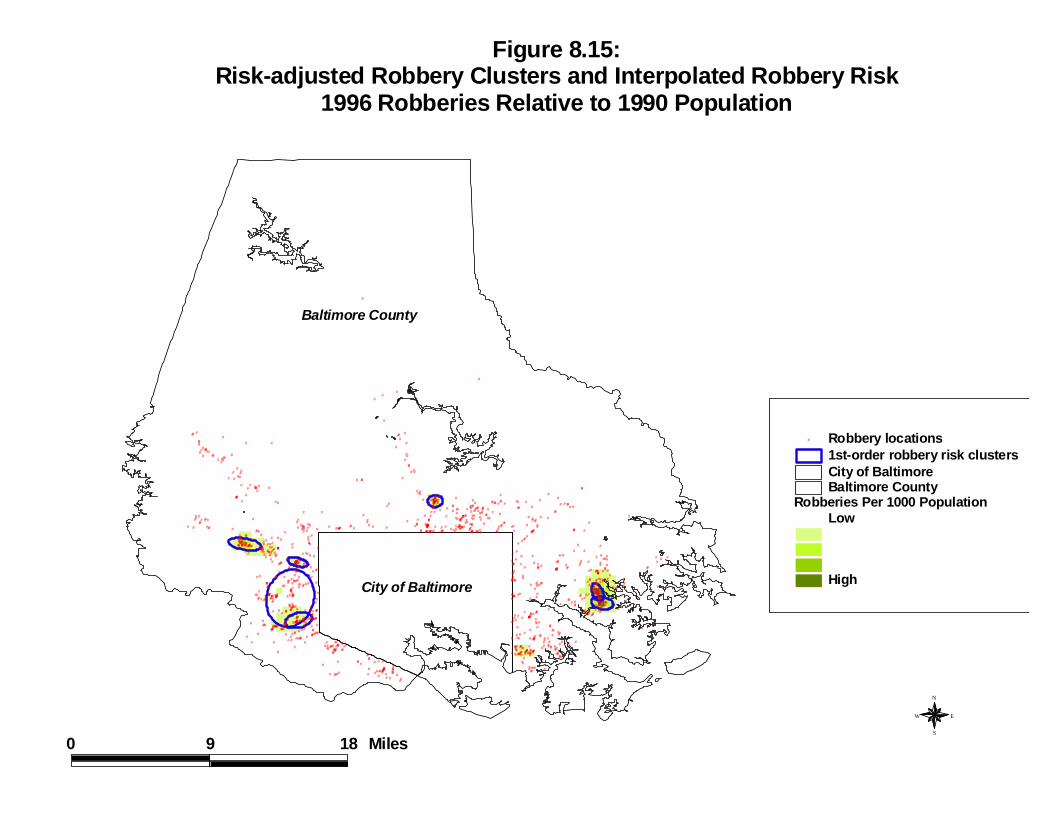
Example 3: Kerne l Dens i ty Est imates and Risk-adjusted Cluster ing o fRobber ies Re lat ive to Populat ion
The fina l example sh ows h ow the duel ker nel in ter pola t ion compa res wit h the r isk -adjust ed nea rest neighbor clust er ing, discussed in cha pt er 6. Figure 8.15 shows 7 first -order r isk-ad just ed clust er s over laid on t he a du el ker nel est ima te of 1996 robberiesrela t ive to 1990 popula t ion .4 As seen , th ere is a cor respondence between the ident ifiedr isk-ad just ed clust er s a nd t he du el ker nel in terpola t ion of the ra t io of robber ies topopula t ion . For a broad r egiona l perspective, th e int erpola t ion pr odu ces a n adequ a temodel of wh er e t her e is a h igh robbery r isk . At the neighborh ood level, however , the r isk -adjust ed clust er s a re m ore specific and would be preferable for use by police in iden t ifyinghigh-r isk loca t ion s.
The advantage of a du a l ker nel dens ity int erpola t ion rou t ine is t ha t two var iablescan be rela ted t ogeth er . By int erpola t ing one var iable to a reference grid a nd t henint erpola t ing a second var iable to the sa me reference grid, the two var iables h ave been

Surface View Contour View
Baltimore Metropolitan Population: 1990Kernel Density Estimate of Block Group Population
-76.90 -76.80 -76.70 -76.60 -76.50 -76.40 -76.30
39.20
39.30
39.40
39.50
39.60
39.70
Ground Level View
N
Figure 8.13:

Surface View Contour View
Baltimore County Vehicle Theft RiskKernel Density Ratio of 1996 Vehicle Thefts to 1990 Population
Ground Level View
N
-76.80 -76.70 -76.60 -76.50 -76.40 -76.30
39.20
39.30
39.40
39.50
39.60
39.70
Figure 8.14:
#
##
#
###
#
##
#
#
#
#
#
#
#
#
###
##
#
#
#
#
#
##
#####
#
###
#
#
#
#
#
####
#
#
#
#####
#
#
#
##
#####
#
#
#
#
#######
#
##
#
#
#
#
##
#
#
#
#
#
#
####
#
#
##
#
#
#
#
#
###
#
#
#
#
#
#
#
#
#
#
#
#
###
#
#
#####
#
##
#
#
#
#
##
#
#
#
#
#
###
#
#
##
#
###
#
##
#
##
##
#
#
#
#
#
#
#
##
#
#
#
###
#
#
#
#
##
#
##
#
#
#
#
#
#
#
#
#
##
#
#######
#
##
#
#
#
#####
#
#
#
#
#
#
##
#
#
##
#
#
#
###
#
#
##
#
###
#
###
#
#
##
#
#
#
#
#
#
###
#
#
###
###
#
#
#
#
#
#
#
#
####
#
#
#
###
#
#
##
#
#
#
#
#
##
#
#
#
##########
#
#
###########
###
#
#
#
##
#
#
####
#
#
#
#
#
#
#
#
#
#
#
#
#
#
#
##
#
##
#
##
#
#
#
##
#
##
#
#
#
#
#
#
#
#
#
#
#
#
#
#
#
#
#
#
#
#
#
#
#
#
#
#
#
#
#
#
#
#
#
#
##
#
#
#
#
#
#
#
#
##
#
#
#
#
#
##
##
#
##
#
#
#
#
#
#
#
##
#
###
##
#
#
#
#
#
#
#
#
#
#
#
#
#
#####
#
#
####
######
#
#
#
###
#
#
#
#
###
#
#
####
#
##
###
###
#
###
##
#
#
##
#
#
###
#
# #
#
#
###
#
#####
#
#
####
#
####
##
#
##
#
#######
#
#
#
###
##
#
#
#
#
#
#
#
##
###
##
#
##
###
##
#
#
#
####
###########
###
#
#
##
#
#
#
#
#
#
##
#
###
############
#
######
#
##
#
######
#
#####
#
#
#
###
##
#
#
#
#
###
#
#######
####
#
##
###
####
#
##
###
#
#
###
###
#
#
#####
##
#
##
#
###
#
#
#
###
##
#
#
#
##
#
#
#####
#
##
#
##
##
#
##
##
#
##
#
##
#
####
#
#
#
#
##
#
#
#
#
#
#
###
#
#
#
#
#
###
##
#
#
#
#
#
#
#
#
#
##
#
##
#
#
#
#
#
#
#
#
#
#
#
#
#
#
#
#
###
#
#
#
#
###
#
#
##
#
#
#
##
#
##
#
##
#
#
#
###
#
####
#
#
##
#
#
#
#
########
#
#
###
#
#
#
#
#
#
#
#
#
#
#
#
##
#
#
##
#
#
###
##
#
#
#
#
####
#
#
#
#
#
#
#
#
##
#
#
#
#
##
#
#
#
####
#
#
#
##
#
##
#
#
##
##
#
#
#
#
#
#
#
#
##
##
#
##
#
#
##
#
########
#
#
###
#
#
#
#
#
#
#
#
#
#
#
#
#
#
#
#
##
#
#
#
##
#
#
#
#
#
###
#
#
##
#
#
#
##
##
#
##
#
#
#
#####
#
#
#
#
#
##
#
#
#
###
#
#
#
#
#
##
#
#
###
#
#
###
#
##
#
####
#
####
#
#
#
###
#
##
###
#####
###
#
#
#
#######
#
##
###
#
#
#
###
###########
#
#
#
##
#
##
#
#
###
#
###
##
#
#
#
##
#
#
###
#
#
#
#
#
#
#
###
#
##
#
#
#
##
##
#
# #
Baltimore County
City of Baltimore
Robberies Per 1000 PopulationLow
High
Baltimore CountyCity of Baltimore1st-order robbery risk clusters
# Robbery locations
0 9 18 Miles
N
EW
S
Figure 8.15:Risk-adjusted Robbery Clusters and Interpolated Robbery Risk
1996 Robberies Relative to 1990 Population

Using Small Area Estimation to Target Health Services
Thomas F. Reynolds, MS University of Texas-Houston School of Public Health
In Texas, the City of Houston and Harris County organized a Public Health Task force to make recommendations concerning the provision of health services for those without health insurance. Task force members wanted to know approximately how many area citizens did not have health insurance. Data from the two most recent Current Population Survey Annual Social and Economic Supplements (CPS-ASEC, 2003-04) were used to derive a synthetic estimate using a stratified model. Estimates were calculated at census tract and block group levels. Selected political divisions were clipped from base maps for political officials and legislators. Percentages are indicative of risk. On the other hand, numbers are essential for targeting physical resources. There is seldom a perfect correspondence between high percentages and large numbers. For example, an area with a concentration of multi-family housing may have a relatively small percentage, but a large number, of uninsured. Percentage maps of the uninsured (figure 1) are generally clustered and informative; however, due to large variations in population numbers at both levels of census geography, maps of the population densities of uninsured proved most valuable to officials (figure 2). CrimeStat was used to develop the density maps. The single kernel density routine was used to estimate the density of block group values using the centroid to represent the values and the number of uninsured as an intensity value. The Moran Correlogram was used to select the type of kernel for the single-kernel interpolation (a uniform distribution) and an optimal bandwidth.
Fig. 1: Percent Uninsured
Fig. 2: Population Density of Uninsured
8.36
int erpola ted t o the sa me geogra ph ica l un its . The two int erpola t ions can then be rela ted, byd ivid ing, subt ract ing, or summing. As has been ment ioned th roughout th is manua l, one ofthe pr oblems with techniques tha t depen d on the concent ra t ion of inciden t s is t ha t theyignore the under lying popula t ion -a t -r isk. With the dua l rou t ine, however , we can st a r t t oexamine the r isk and not jus t the concen t ra t ion .
Visua lly P resen ting Kernel Est imate s
Whet her the single- or du el-ker nel es t imate is u sed, t he r esu lt is a gr idin ter pr et a t ion of th e da ta . By sca ling these va lues by color in a GIS progra m, avisualiza t ion of the data i s obta ined. Areas with higher densit ies can be shown in darkertones and those wit h lower densit ies can be shown in ligh ter tones; some people do theopposit e wit h the h igh densit y area s bein g lighter .
To make the visua liza t ion even more rea list ic, one could use a GIS progr am to cutou t those gr id cells tha t are ou t s ide the s tudy a rea or a re on water bod ies . Before doingth is , h owever , be sure to re-sca le the est im ated “Z” va lu es so tha t they will sum to the tota lof the origin a l gr id. For exa mple, if the origin a l sa mple size was 1000, t hen the gr id cellswill su m to 1000 if th e absolu te den sit y opt ion is chosen . If, say, 20% of th ese cells a rethen removed to impr ove th e visu a liza t ion , th en the grid cell Z values h ave to be re-sca ledso th a t their sum will con t inu e to be 1000. A simple way to do th is is to, firs t , add up t he Zva lu es for the remain in g cells and, second, m ult ip ly ea ch gr id cell Z by t he ra t io of theoriginal sum t o th e reduced sum.
Th e visua liza t ion is useful for a br oad, r egiona l view. It is not par t icu la r ly usefulfor m icro an alysis. The use of one of th e cluster r out ines discussed in cha pters 6 an d 7would be m ore appropr ia te for sm all a rea ana lysis .
Conclusion
Kernel den sit y est imat ion is one of the ‘moder n’ spa t ia l st a t ist ical t echniqu es . Ther e is cur ren t ly resea rch on the u se of th is t echn ique in both the st a t ist ical t heory a nd indevelopin g a pplica t ion s. F or cr im e ana lysis , t he technique represen t s a power fu l way ofconduct ing both ‘hot spot ’ ana lys is as well a s being able to link the ‘hot spot s ’ to anunder lying popula t ion-a t -r isk. It can be used both for police deploymen t by ta rgeting ar easof h igh concen t ra t ion of inciden t s as well a s for p reven t ion by t a rget ing a reas with h ighr isk. I t can a lso be used as a research tool for ana lyzing t wo or more dis t r ibu t ion s. Moredevelopm ent of th is appr oach can be expected in t he next few years.

The Risk of Violent Incidents Relative to Population Density in Cologne Using the Dual Kernel Density Routine
Dietrich Oberwittler and Marc Wiesenhütter
Max Planck Institute for Foreign and International Criminal Law Freiburg, Germany
When estimating the density of street crimes within a metropolitan area by interpo-
lating crime incidents, the result is usually a very high concentration in the city center. However, there is also a very high concentration of people either living or pursuing their daily routine activities in these areas. The question emerges how likely is a criminal event when taking into account the number of people spending their time in these areas. The CrimeStat duel kernel density routine is able to estimate a ratio density surface of crime relative to the 'population at risk'.
In this example, data on ‘calls to the police’ for assault and battery from April 1999 to
March 2000 (N=6363 calls) and population from Cologne were used. Exact information on the number of people spending their time in the city does not exist. Therefore, 1997 counts of passengers entering and leaving the public transport system at each of 550 stations and bus stops in the city was used as a proxy variable. The number of persons at each station or bus stop was assigned to adjacent census tracts and added to the resident population resulting in a crude measure of the 'population at risk'.
In the dual kernel routine, the density estimate of crime incidents is compared to the
density estimate of the population at risk, defined by the centroids of census tracts with the number of persons as an intensity variable. We chose the normal method of interpolation and adaptive intervals with a minimum of five points. The adaptive bandwidth adjusts for the fact that there are fewer incidents and census tracts at the edges of the city, resulting in a relatively smoother density surface for the ratio. The results were output to ArcView.
The effect of adjusting the crime distribution for the underlying 'population at risk'
becomes quite visible. Whereas the concentration of crime is highest in the city center (left map), the crime risk (right map) is in fact much higher in several more distant areas that are known for high concentrations of socially disadvantaged persons. Given the imperfect nature of the population data these results should be interpreted as a broad view on the distribution of crime risk that, nevertheless, has important policy implications. Single kernel density of crime incidences
(assault & battery, Cologne 1999/2000) Dual kernel density of crime incidences relative to population at risk
Kernel Density Interpolation of Police Confrontations in
Buenos Aires Province, Argentina: 1999
Gastón Pezzuchi Crime Analyst
Buenos Aires Province Police Force Buenos Aires, Argentina
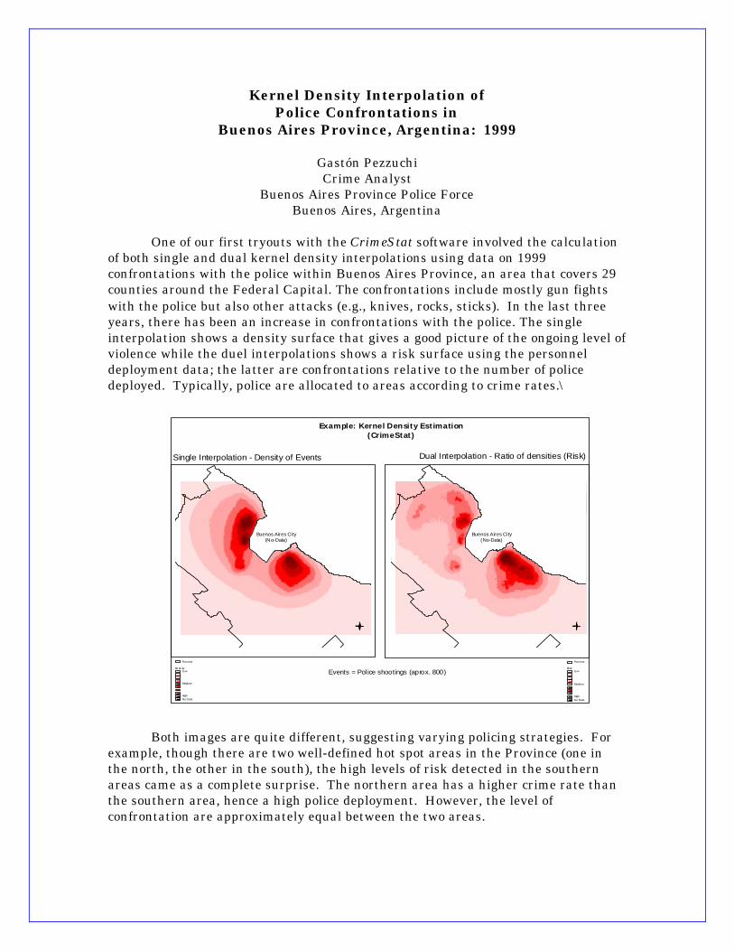
One of our first tryouts with the CrimeStat software involved the calculation
of both single and dual kernel density interpolations using data on 1999 confrontations with the police within Buenos Aires Province, an area that covers 29 counties around the Federal Capital. The confrontations include mostly gun fights with the police but also other attacks (e.g., knives, rocks, sticks). In the last three years, there has been an increase in confrontations with the police. The single interpolation shows a density surface that gives a good picture of the ongoing level of violence while the duel interpolations shows a risk surface using the personnel deployment data; the latter are confrontations relative to the number of police deployed. Typically, police are allocated to areas according to crime rates.\
Events = Pol ice shootings (aprox. 800)
Buenos Aires City(No-Data)
Buenos Aires City(No-Data)
Example: Kernel Density Estimation(CrimeStat)
Single Interpolation - Density of Events Dual Interpolation - Ratio of densities (Risk)
N N
De ns ityLo w
Medium
HighNo Data
Fron tera
RiskLo w
Medium
HighNo Data
Fron tera
Both images are quite different, suggesting varying policing strategies. For example, though there are two well-defined hot spot areas in the Province (one in the north, the other in the south), the high levels of risk detected in the southern areas came as a complete surprise. The northern area has a higher crime rate than the southern area, hence a high police deployment. However, the level of confrontation are approximately equal between the two areas.

Evolution of the Urbanization Process in the Brazilian Amazonia
Silvana Amaral, Antônio Miguel V. Monteiro, Gilberto Câmara, José A. Quintanilha INPE, Instituto Nacional de Pesquisas Espaciais, Brazil
The Brazilian Amazon rain forest is the world’s largest contiguous area of
tropical rain forest in the world. During the last three decades, the region has experienced the largest urban growth rates in Brazil, a process that has reorganized the network of human settlements in the region. We used the CrimeStat single and duel kernel density routines to visualize trends in urbanization from 1996 to 2000 in Amazonia. Two variables were used to measure urbanization: 1) the concentration of urban nuclei (city density); and 2) the ratio of urban to total population.
The concentration of cities was spatially associated withfederal roads in the
eastern and southern portions, and along the Amazonas River in the middle of the region. Additionally, the surfaces of urban population show that city density is not always associated with large urban populations. From 1996 to 2000 city density increased in the western Amazonia (Pará state) at a greater rate than the growth of the urban population. In the southeastern part of the region (Rondônia state), there were many urban centers. But the ratio of urban to total population was small, indicating that they are predominately agricultural regions.
Urban Pop/Total Pop-1996
City density - 2000
City density - 1996
Urban Pop/Total Pop-2000

8.40
1. Ther e a re differ en ces in opinion about how wide a pa r t icula r fixed bandwidt hsh ould be determined. The sm ooth ing is done for a dist r ibut ion of values, Z. If thereare on ly un ique point s (an d, hen ce, th ere is no Z value a t a poin t ), th e dist ancesbetween point s can be subs t itu ted for Z. Thus, Mean D is th e mea n distance, sd(D)is the st andard devia t ion of dis t ance, a nd iqr (D) is the in ter -quar t ile range ofdis tances between poin t s. These would be subst it u ted for MeanZ, sd(Z), a nd iqr (Z)respectively
Silverman (1986; 45-47; Härdle, 1991; Farewell, 1999) proposed a ba ndwidth , h , of:
iqr (Z)h = 1.06 * min { sd(Z), -------- } * N -1 /5
1.34
where m in is t he m in imum of the n ext two ter ms, sd(Z) is the st andard devia t ion ofthe va r iable, Z, bein g in ter pola ted, iqr(Z) is t he in ter -qua r t ile r ange of Z, and N isthe sample size.
Bowman and Azza lin i (1997; 31) defin ed a sligh t ly differen t opt im al bandwid th for anorm al ker nel.
4h = { --------- }1 /5 * sd(Z)
3N
To avoid bein g influen ced by out lier , they su ggest ed usin g the m edian absolu tedevia t ion est im ator for sd(Z)
Z(i) - MedianZMAD(Z) = media n{ --------------------- }
0.6745
Scot t (1992) suggested an upper bound on the normal k ernel of
h = 1.144 * sd(Z) * N -1 /5
Bailey a nd Gat rell (1995, 85-87) offered a rough choice for the bandwid th of
h = 0.68 * N -0.2
but suggested tha t the user could exper im ent wit h differen t bandwid ths to explor ethe su r face.
On the oth er hand, t he concept of an ada pt ive bandwidt h is ba sed m ore on sa mplin g
En dn ot e s t o Ch ap te r 8

8.41
theory (Bailey and Ga t rell, 1995). By increa sing th e ban dwidt h un t il a fixednumber of poin t s a re counted ensures tha t the level of precis ion is constan tth roughout th e region. As with all sam pling, th e stan dar d error of th e estima te is afunct ion of the sample s ize; a la rger sample leads to smaller er ror . In genera l, ifthere was in dependent sampling, the 95% confidence in terva l of a bandwid th for anormal ker nel cou ld be appr oximated by
.595% C.I . = Mean(Z) +/- 1.96 * --------- * sd(Z)
N(h)1 /2
wh er e N(h) is t he ada pt ive sa mple size (the number of point s counted wit h in thebandwidt h for the ada pt ive ker nel). This a ssu mes t ha t a poin t has a n equa llikelihood of fallin g with in the ba ndwidt h of one cell compa red to an adjacent cell(i.e., it sit s on the bounda ry of th e ba ndwidt h circle). The ada pt ive bandwidt hcr iter ia r equires tha t the ban dwidt h be increa sed u n t il it captures t he specifiednumber of poin t s. On average, if there a re N poin t s in a region of area , A, a nd if t heada pt ive sa mple size is N(p), then the average a rea requ ired to capt ure N(p) poin t sis
N(p) * AA(p) = --------------
N
and t he average ba ndwidt h , Mea n(h), is
A(p) N(p) * AMean(h) = SQRT[------------] = SQRT[ ---------------]
B N*B
Each of th ese provide differ en t crit er ia for the ba ndwidt h size wit h the a da pt ivebein g the m ost conservat ive. For exa mple, for a st anda rdized dis t r ibu t ion wit h1000 dat a points, a sta nda rdized mean of Z of 0 and a sta nda rdized stan dar ddevia t ion of 1, the Silverman cr it er ia would produce a ba ndwidth of 0.2663; theBowman and Azza lin i cr it er ia would produce a bandwid th of 0.2661; the Scot tcrit er ia would pr oduce a bandwidt h of 0.2874 and t he Ba iley and Gat rell crit er iawould pr odu ce a bandwidt h of 0.1708. For t he ada pt ive int erval, if the requiredada pt ive sa mple size is 25, t hen the average ba ndwidt h would be a pproximately0.3162 (th is assu mes t ha t the area is a circle with a radius of 2 st anda rdizedst anda rd devia t ions ).
2. Crim eS tat will ou tpu t the geogr aphica l boundar ies of the reference gr id (a polygongrid) an d will a ssign a th ird -var iable (ca lled Z ) as the densit y est im ate. Of thethree polygon gr id ou tpu t s, ArcView ‘.shp’ files can be read dir ect ly in to thep rogram. For MapIn fo, on the other hand, the ou tpu t is in MapInfo In terchangeForm at (a ‘.mif’ an d a ‘.mid’ file); th e density estima te (also called Z ) is assigned to
8.42
the ‘.m id’ file. The files must be im por ted to conver t it to a MapIn fo ‘.t ab’ file. F orAtlas*GIS ‘.bna’ format , however , there a re two files tha t are ou tpu t - a ‘.bna’ filewhich includes t he bounda r ies of the polygon grid a nd a ‘.dbf’ file which includes t hegrid cell na mes (called gridcell) an d th e density estima te (also called Z ). The ‘.bna ’file must be read in fir st and then the ‘.dbf’ file must be read in and matched to theva lu e of gridcell. For a ll th ree out put form at s, th e values of Z can be shown as athemat ic m ap bu t the ranges must be adjusted to illu st ra te the likely loca t ion s forthe offender ’s r esidence (i.e., the defau lt values in the GIS programs will not d isp laythe densit ies very well). On the other hand, t he defau lt in terva l va lu es for S urferfor Windows an d ArcView S pat ial Analyst provide a reasonably good visua liza t ion ofth e densities.
3. All the Crim eS tat outpu t s except for ArcView ‘sh p’ files ar e in ASCII. There areusu a lly ‘edge effects ’ and va lues in ter pr et ed out side t he a ctu a l geograph ical a rea . These can be rem oved with an ASCII ed itor by su bst itu t ing ‘0' for the values a t theedges or ou t side t he st udy region . For ‘sh p’ files, the values a t the edges can beedited with in t he ArcView progra m. Anoth er altern at ive is to ‘cut out ’ th e cells th ata re beyond t he study a rea . Care m ust be t aken , however , to not edit an out pu t filetoo much otherwise it will bear lit t le rela t ionsh ip to the ca lcu lat ed kernel est ima te.
4. The r isk-adju sted h iera rch ica l cluster in g (Rnnh) method defin ed the la rgest sea rchradius bu t a minim um of 25 point s being r equired to be clus tered. The k ernelest im ate for both the Rn nh and the duel-k ernel r out in es used the normaldistr ibut ion fun ction with a n a dapt ive ban dwidth of 25 points.