crop ground cover fraction and canopy … ground cover fraction and canopy chlorophyll content...
TRANSCRIPT
CROP GROUND COVER FRACTION AND CANOPY CHLOROPHYLL CONTENT
MAPPING USING RAPIDEYE IMAGERY
E. Zillmann a, M. Schönerta, H. Lilienthalb, B. Siegmannc, T. Jarmerc, P. Rossoa, H. Weichelt a
a BlackBridge, Dept. of Application Research, 10719 Berlin, Germany - ([email protected]) b Julius-Kühn-Institute (JKI), Federal Research Centre for Cultivated Plants, 38116 Braunschweig, Germany –
([email protected]) cInstitute for Geoinformatics and Remote Sensing, University of Osnabrueck, 49076 Osnabrueck, Germany – ([email protected]
osnabrueck.de)
KEY WORDS: Ground Cover, Canopy Chlorophyll Content, RapidEye, Spatial Variability, Precision Agriculture
ABSTRACT:
Remote sensing is a suitable tool for estimating the spatial variability of crop canopy characteristics, such as canopy chlorophyll
content (CCC) and green ground cover (GGC%), which are often used for crop productivity analysis and site-specific crop
management. Empirical relationships exist between different vegetation indices (VI) and CCC and GGC% that allow spatial
estimation of canopy characteristics from remote sensing imagery. However, the use of VIs is not suitable for an operational
production of CCC and GGC% maps due to the limited transferability of derived empirical relationships to other regions. Thus, the
operational value of crop status maps derived from remotely sensed data would be much higher if there was no need for re-
parametrization of the approach for different situations.
This paper reports on the suitability of high-resolution RapidEye data for estimating crop development status of winter wheat over
the growing season, and demonstrates two different approaches for mapping CCC and GGC%, which do not rely on empirical
relationships. The final CCC map represents relative differences in CCC, which can be quickly calibrated to field specific conditions
using SPAD chlorophyll meter readings at a few points. The prediction model is capable of predicting SPAD readings with an
average accuracy of 77%. The GGC% map provides absolute values at any point in the field. A high R² value of 80% was obtained
for the relationship between estimated and observed GGC%. The mean absolute error for each of the two acquisition dates was 5.3%
and 8.7%, respectively.
1. INTRODUCTION
Remote sensing is a suitable tool for estimating the spatial
variability of crop canopy characteristics such as green ground
cover (GGC%) and canopy chlorophyll content (CCC). Both
variables are often used for crop productivity analysis and site-
specific crop management. Spatially high-resolution crop
growth status information can provide farmers with relevant
information e.g. for site-specific application of fertilizer (Scharf
and Lory, 2002, Emerine, 2006), growth regulator (Maas et al.
2004), irrigation requirements (Hunsaker et al., 2005, Er-Raki,
2010), and crop productivity analysis (Schulthess et al., 2013).
Since field management decisions are often time-critical, an
almost real time production and provision of spatially high-
resolution CCC and GGC% maps is desired.
Leaf chlorophyll absorption in the visible part of the
electromagnetic spectrum provides the basis for using remotely
sensed reflectance as a tool for the determination of crop
development status. Often spectral vegetation indices (VI) are
used to derive crop status information. Several studies have
proven the existence of empirical relationships between
different VIs and both CCC and GGC%. Even though the
normalized difference vegetation index (NDVI) (Rouse et al.
1973) is the most commonly used VI, it has the limitation that it
tends to saturate when LAI exceeds 2, and it is also strongly
influenced by soil background conditions (Baret et al., 1991).
Several other VIs have been proposed for estimating CCC of
various crops (Daughtry et al., 2000, Haboudane et al., 2002).
In particular, the red-edge region of the spectrum showed
strong potential for estimating canopy chlorophyll content. The
main advantage of red-edge based indices is their reduced
saturation effect due to a lower absorption by the chlorophyll in
the red-edge spectral region compared to the red spectrum
(Gitelson and Merzlyak, 1996). Thus, red-edge based indices
are still sensitive to chlorophyll absorption at higher crop
canopy densities. Since CCC varies widely over the growing
season and among crops, any VI requires a large dynamic range
for chlorophyll estimation. Eitel et al., (2007) have proven the
general suitability of the RapidEye red-edge band for CCC
estimation in winter wheat.
Accordingly, BlackBridge (as the owner and distributor of
RapidEye data) has been using the Normalized Difference Red-
Edge Index (NDRE) (Barnes et al., 2000), to produce relative
chlorophyll maps. Although these maps are known to reflect the
variability of CCC within individual fields, the variable nature
of the NDRE-Chlorophyll relationship in different situations,
has prevented the establishment of a universal relationship for
estimating actual CCC values on the field. This limited
transferability of empirical relationships hinders its
incorporation into operational production processes.
One option to overcome this limitation is to explore the
possibility of establishing a relationship NDRE-CCC on a case
by case basis, but with a procedure that is simple enough to be
applied by farmers with little effort and previous knowledge.
With this goal in mind, in this study a test was performed to
determine the accuracy of NDRE maps as predictors of values
of CCC when using a set of a few measurements on the ground.
Often VIs used for fractional GGC% estimation rely on the soil
line in the red and near-infrared (NIR) spectral feature space.
Richardson and Wiegand (1977) introduced the bare soil line
concept to improve the discrimination between bare soil and
sparse vegetation cover. In particular the weighted difference
vegetation index (WDVI) (Clevers, 1988) and the perpendicular
vegetation index (PVI) (Jackson et al., 1980) were successfully
The International Archives of the Photogrammetry, Remote Sensing and Spatial Information Sciences, Volume XL-7/W3, 2015 36th International Symposium on Remote Sensing of Environment, 11–15 May 2015, Berlin, Germany
This contribution has been peer-reviewed. doi:10.5194/isprsarchives-XL-7-W3-149-2015
149
tested to estimate GGC% from multi-spectral imagery (Bouman
et al., 1992, Schulthess et al., 2013, Maas et al., 2008, Rajan et
al., 2009).
Even though the basic concept of the PVI is to reduce the
influence of bare soil reflection, this index cannot be considered
fully insensitive to soil brightness. Huete et al. (1985) found out
that for same amounts of vegetation cover PVI shows lower
values on dark soils than on bright soils. Moreover, the initial
assumption of an existing “global” soil line encompassing a
wide range of soil conditions has been disproved. Soil type
specific conditions cause variations in the slope and intercept of
the soil line, and consequently influence the value of the
particular VI (Huete et al., 1985). Therefore, regional specific
soil lines are necessary to enable accurate GGC% estimation by
utilizing soil line based VIs.
Maas et al. (2008) developed a non-empirical and self-
calibrating approach for estimating GGC% based on the bare
soil line and full canopy point (FCP) reflectance. The FCP is
defined as the canopy reflectance in the NIR and the red
spectral band at 100% ground coverage when seen directly
from above. With parameters derived from the scatterplot of the
NIR vs. the red band values of a particular multi-spectral image,
they achieved a GGC% estimation error below 6% on average.
The operationalization of this approach for the GGC% map
production relies on the automated determination of an
adequate soil line and FCP in each particular image, which is
highly error-prone without a proper image screening
beforehand. The accidental inclusion of urban areas, lakes,
clouds and cloud shadows prevents the accurate identification
of the soil line (Maas et al., 2008, Xu et al., 2013). Therefore,
one of the goals of the study reported here is to find a procedure
to improve the automatic extraction of a soil line representative
of the area under study.
The identification of the FCP requires the existence of full
canopy within the image, which is not guaranteed for
acquisitions early and late in the season. Furthermore, leaves
transmit and reflect light in the NIR spectrum and absorb only a
small fraction. As a result, the NIR reflection for a pixel of full
canopy can continue to increase with increasing leaf density.
Thus, it is very likely that automatically extracted NIR values
are above the normal values of full canopy. To overcome this
challenge, the use of an empirical FCP is recommended (Maas
et al., 2008).
The aim of this work is to demonstrate the feasibility of the
automated generation of relative canopy chlorophyll maps
(CCC) and absolute GGC% maps for individual fields based on
RapidEye imagery, with the least amount of manual
intervention. The resulting maps were compared to
corresponding ground truth measurements of chlorophyll
content and GGC% to assess the accuracy. The produced maps
provide information about the spatial variability of crop growth
that has potential use in precision agriculture as a means for
directed field scouting and variable rate management.
2. MATERIALS AND METHODS
2.1 Study Area
The study area is located in the federal state of Saxony-Anhalt,
Germany (11°54′E, 51°47′N) in an intensively used agricultural
landscape. The region is characterized by Chernozem in
conjunction with Cambisols and Luvisols as the predominant
soil types of the Loess covered Tertiary plain. The test site is
characterized by highly variable spatial soil properties. Within
the study area, one winter wheat (Triticum aestivum L) field
with a size of 90 ha was selected for the assessment of wheat
CCC and GGC%. The field showed two areas with no
vegetation as a result of waterlogging in early spring 2011.
2.2 Field Measurements and Data Extraction
Field data were collected close to image acquisition on the 8th
of May and 22nd of June 2011. The first campaign was
conducted within one day of image acquisition to avoid any
distortions of the results due to high daily growth rates at this
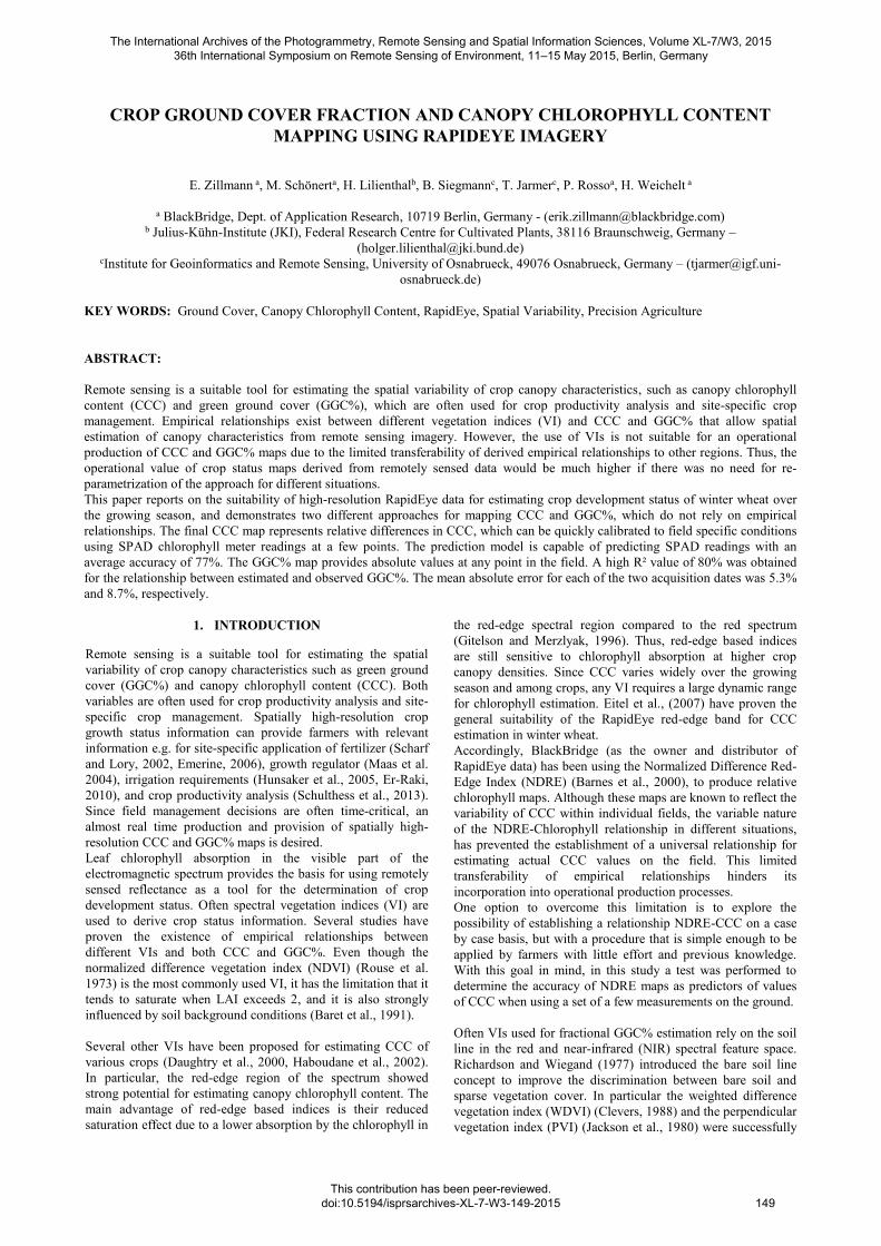
stage of crop development. The sample locations were defined
aiming at covering the entire crop variability within the field as
described in Siegmann et al. (2013). A total number of 24 and
18 sample plots were measured at winter wheat’s stem
elongation and early ripening stage, respectively (Figure 1).
Figure 1. Test site with the sampling locations measured on 8th
of May (dark) and 22nd of June 2011 (bright). The
image shows the situation on the 7th of May 2011.
2.2.1 Ground Measurements of Chlorophyll
Field data collection included leaf area index (Licor LAI-
2200©, Delta-T Sunscan©) and leaf chlorophyll meter readings
in the upper canopy (Minolta SPAD-502©). SPAD
measurements represent a unit-less relative measurement of leaf
chlorophyll content and have been proven to be positively
correlated to chlorophyll content of wheat (Reeves et al., 1993)
and other crops (Zhu et al., 2012).
Since satellite images represent the spectral reflectance from 3-
dimensional crop canopies, the SPAD readings at leaf level
were also transformed to a 3-dimensional CCC. The CCCSPAD
was derived by calculating the product of the corresponding
leaf SPAD reading and leaf area index (Gitelson et al., 2005).
Samples showed a considerable CCCSPAD range from 18 at
minimum to 151 at maximum on the 8th of May 2011 and from
20 at minimum to 240 at maximum on the 22nd of June. The
average CCCSPAD from the two dates ranged from 58 to 119.
2.2.2 Ground Measurements of Ground Cover
Photographs of the wheat canopy were taken with a standard
digital camera looking downward from a distance of
approximately 1.5 m to allow the estimation of green crop
ground cover. Photographs were subject to supervised
classification aiming at the objective determination of reference
GGC%. Trimble eCognition Developer 8© software was used to
perform an object-based supervised classification of green
vegetation and non-green vegetation. The image was cropped to
include only the central portion for the GGC% determination to
minimize the effects of optical distortions on the plant canopy
present near the edges of the image. GGC% was calculated as
The International Archives of the Photogrammetry, Remote Sensing and Spatial Information Sciences, Volume XL-7/W3, 2015 36th International Symposium on Remote Sensing of Environment, 11–15 May 2015, Berlin, Germany
This contribution has been peer-reviewed. doi:10.5194/isprsarchives-XL-7-W3-149-2015
150
the area of green vegetation of the resulting polygon shape file
divided by the total area of the photograph.
The mean reference GGC% of the field was 71% on the 8th of
May and 65% on the 22nd of June 2011. The variability of
GGC% observed was considerably higher in June ranging from
23% at minimum and 95% at maximum compared to 42% at
minimum and 96% at maximum in May.
2.3 Remote Sensing Data Processing
2.3.1 Satellite Imagery
The RapidEye (RE) satellite system is a constellation of five
identical earth observation satellites with the capability to
provide large area, multi-spectral images with frequent revisits
in high resolution (6.5 m at nadir). In addition to the blue (440–
510 nm), green (520–590 nm), red (630–685 nm) and NIR
(760–850 nm) bands, RapidEye has a red-edge band (690–
730 nm), especially suitable for vegetation analysis. The
RapidEye level 3A standard product covers an area of
25x25 km, and is radiometrically calibrated to radiance values
(Anderson et al. 2013), ortho-rectified, and resampled to 5 m
spatial resolution. All the images used were calibrated to top of
atmosphere reflectance. The two images used (Tile ID
3363006) for crop status mapping were acquired on the 7th of
May and 27th of June 2011.
2.3.2 Chlorophyll Mapping
Since the relationship between canopy chlorophyll and the
spectral VI used may vary between crop types or different areas,
it is more appropriate to restrict the comparisons to individual
crop fields. For this reason, the Chlorophyll Map focuses on
differences within single fields, thus providing a relative
chlorophyll level scale.
The NDRE was calculated for the entire satellite image (1), as:
NDRE = (ρNIR – ρREdge) / (ρNIR + ρREdge) (1)
where ρNIR and ρREdge are the reflectance values of the near
infrared and red-edge spectral region.
The NDRE layer obtained was clipped to the test field area and
all included pixels were encoded as a relative chlorophyll level
index (RCLI) into a 0 – 100 grey value scale.
The relative chlorophyll values were calibrated to the field
specific conditions by obtaining three ground measurements of
CCCSPAD for each of the three chlorophyll level (low, moderate
and high) areas previously delineated. A linear regression
analysis between the CCCSPAD values and the corresponding
relative chlorophyll map values allowed for generating a linear
transfer function to be applied to the relative chlorophyll map in
order to estimate the spatial distribution of CCC.
2.3.3 Green Ground Cover Mapping
Green ground cover (GGC) is defined as the fraction of an area
covered with green plant canopy. GGC percent maps are
generated based on a modification of the original approach
developed by Maas et al. (2008). The required bare soil line
slope and intercept were obtained by calculating the arithmetic
mean from automatically generated soil lines of a set of multi-
temporal images using the slightly modified procedure from
Fox et al. (2004). Images before and after the main vegetation
period were used to guarantee a sufficient number of pixels
representing bare soil. The empirical FCP reflectance was
determined by averaging the reflectance values from multiple
locations within the field known to be more than 90% covered
with vegetation at the time of image acquisition.
The GGC% (2) was calculated from the ratio of the PVI (3)
value to the corresponding full-canopy PVI (PVIFC) value (4)
as:
GGC% = PVI / PVIFC (2)
where
PVI = (ρNIR – a * (ρRed)) –b) / (1 + a²)0.5 (3)
and
PVIFC = (ρNIRFC – a * (ρRedFC)) –b) / (1 + a²)0.5 (4)
in which a and b are the slope and the intercept of the bare soil
line respectively; and ρNIR and ρred are the reflectance values
of the corresponding spectral band.
The final GGC% map expresses the percentage of ground
covered by the crop green foliage (0%, no green vegetation, and
100%, ground entirely covered with green vegetation).
2.4 Accuracy Assessment
The sampling points were buffered with a radius of 10 m to
extract the average estimated CCC (CCCest) and GGC% values
which were then stored in a shape file for subsequent analysis.
Linear regression analysis between CCCest and ground
measured CCCSPAD, as well as between the estimated and
observed GGC% was performed to assess the estimation
accuracy, respectively.
3. RESULTS AND DISCUSSION
Correlation analysis between the CCCSPAD data obtained during
the field sampling campaign and six spectral VIs derived from
multi-spectral RapidEye imagery revealed best correlations for
those indices incorporating the red-edge reflection (Table 1).
The results revealed strong linear correlation between CCCSPAD
and NDRE and CIred-edge for two different development stages of
winter wheat.
Table 1. Correlation coefficient (r) between CCCSPAD of winter
wheat and selected vegetation indices (n=24 in May;
n=18 in June; level of significance, p = 0.01).
Date NDRE MCARI MTVI2 CIred-edge OSAVI NDVI
May 2011 0.90 0.63 0.89 0.90 0.89 0.86
June 2011 0.87 0.82 0.87 0.87 0.87 0.86
MCARI (Daughtry et al., 2000), MTVI2 (Haboudane et al., 2004),
CIred-edge (Gitelson et al., 2003), OSAVI Rondeaux et al., 1996)
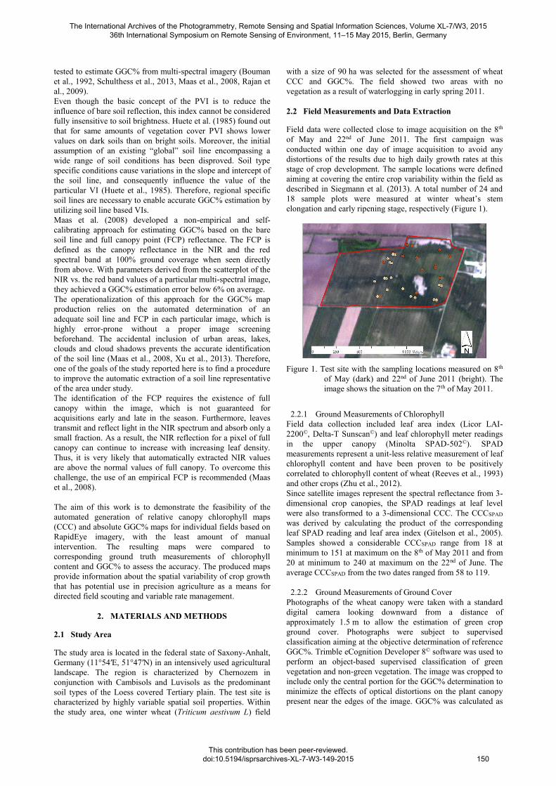
Figure 2 shows the generated RCLI map for the winter wheat
field on 7th of May 2011. The dimensionless chlorophyll levels
are represented in eight classes of colour tones representing
relative differences in chlorophyll content within the field.
Figure 2. Spatial distribution of classes representing relative
chlorophyll level differences in winter wheat on 7th
of May 2011.
The International Archives of the Photogrammetry, Remote Sensing and Spatial Information Sciences, Volume XL-7/W3, 2015 36th International Symposium on Remote Sensing of Environment, 11–15 May 2015, Berlin, Germany
This contribution has been peer-reviewed. doi:10.5194/isprsarchives-XL-7-W3-149-2015
151
This relative map provides accurate information about the
spatial variability of CCC within the field and facilitates
directed field scouting to obtain SPAD and LAI measurements
in specific areas of the field. These measurements allow for the
calibration the RCLI map to field condition specific CCCSPAD
values and enables the farmer to make in-season N fertilization
rate decisions and applications.
Three CCCSPAD measurements corresponding to each of the
three classes representing high, moderate, and low relative
chlorophyll levels were selected and used to calibrate the
relative chlorophyll values to CCCSPAD values. The relationship
between relative chlorophyll levels and CCCSPAD for both dates
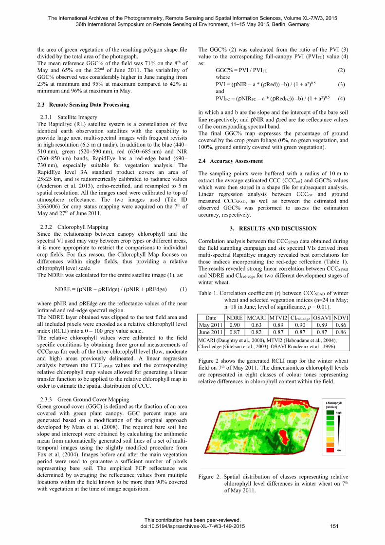
is shown in Figure 3-A and Figure 4-A, respectively.
The derived linear transfer function was then used to estimate
the spatial variability of CCC based on relative chlorophyll
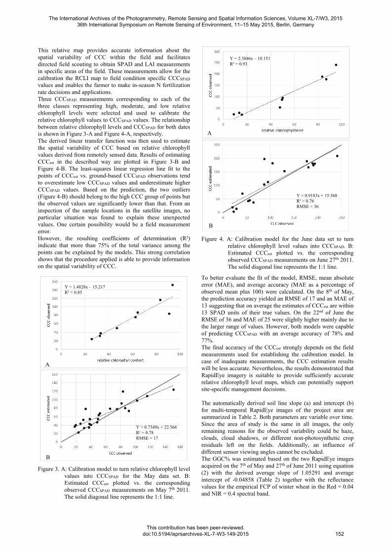
values derived from remotely sensed data. Results of estimating
CCCest in the described way are plotted in Figure 3-B and
Figure 4-B. The least-squares linear regression line fit to the
points of CCCest vs. ground-based CCCSPAD observations tend
to overestimate low CCCSPAD values and underestimate higher
CCCSPAD values. Based on the prediction, the two outliers
(Figure 4-B) should belong to the high CCC group of points but
the observed values are significantly lower than that. From an
inspection of the sample locations in the satellite images, no
particular situation was found to explain these unexpected
values. One certain possibility would be a field measurement
error.
However, the resulting coefficients of determination (R²)
indicate that more than 75% of the total variance among the
points can be explained by the models. This strong correlation
shows that the procedure applied is able to provide information
on the spatial variability of CCC.
Figure 3. A: Calibration model to turn relative chlorophyll level
values into CCCSPAD for the May data set. B:
Estimated CCCest plotted vs. the corresponding
observed CCCSPAD measurements on May 7th 2011.
The solid diagonal line represents the 1:1 line.
Figure 4. A: Calibration model for the June data set to turn
relative chlorophyll level values into CCCSPAD. B:
Estimated CCCest plotted vs. the corresponding
observed CCCSPAD measurements on June 27th 2011.
The solid diagonal line represents the 1:1 line.
To better evaluate the fit of the model, RMSE, mean absolute
error (MAE), and average accuracy (MAE as a percentage of
observed mean plus 100) were calculated. On the 8th of May,
the prediction accuracy yielded an RMSE of 17 and an MAE of
13 suggesting that on average the estimates of CCCest are within
13 SPAD units of their true values. On the 22nd of June the
RMSE of 36 and MAE of 25 were slightly higher mainly due to
the larger range of values. However, both models were capable
of predicting CCCSPAD with an average accuracy of 78% and
77%.
The final accuracy of the CCCest strongly depends on the field
measurements used for establishing the calibration model. In
case of inadequate measurements, the CCC estimation results
will be less accurate. Nevertheless, the results demonstrated that
RapidEye imagery is suitable to provide sufficiently accurate
relative chlorophyll level maps, which can potentially support
site-specific management decisions.
The automatically derived soil line slope (a) and intercept (b)
for multi-temporal RapidEye images of the project area are
summarized in Table 2. Both parameters are variable over time.
Since the area of study is the same in all images, the only
remaining reasons for the observed variability could be haze,
clouds, cloud shadows, or different non-photosynthetic crop
residuals left on the fields. Additionally, an influence of
different sensor viewing angles cannot be excluded.
The GGC% was estimated based on the two RapidEye images
acquired on the 7th of May and 27th of June 2011 using equation
(2) with the derived average slope of 1.05291 and average
intercept of -0.04858 (Table 2) together with the reflectance
values for the empirical FCP of winter wheat in the Red = 0.04
and NIR = 0.4 spectral band.
A
B
A
B
Y = 0.7349x + 22.566
R² = 0.78
RMSE = 17
Y = 1.4828x – 15.217
R² = 0.85
Y = 0.9183x + 15.568
R² = 0.76
RMSE = 36
Y = 2.3846x – 18.151
R² = 0.93
The International Archives of the Photogrammetry, Remote Sensing and Spatial Information Sciences, Volume XL-7/W3, 2015 36th International Symposium on Remote Sensing of Environment, 11–15 May 2015, Berlin, Germany
This contribution has been peer-reviewed. doi:10.5194/isprsarchives-XL-7-W3-149-2015
152
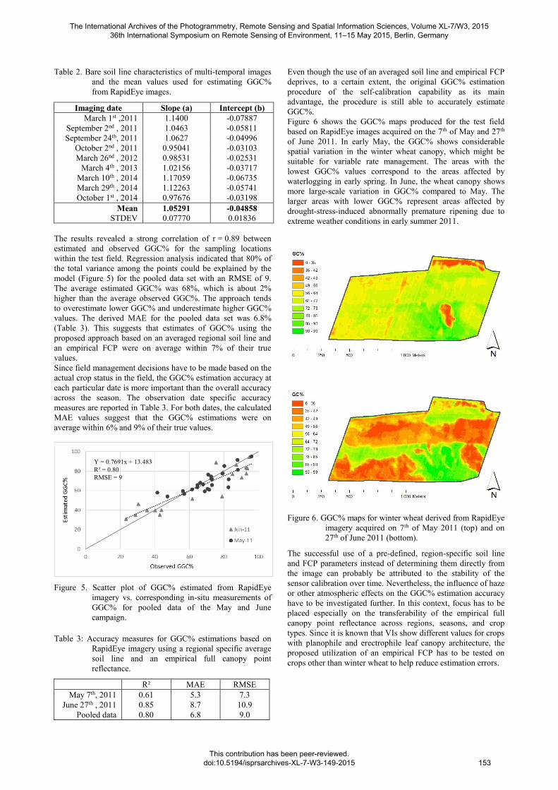
Table 2. Bare soil line characteristics of multi-temporal images
and the mean values used for estimating GGC%
from RapidEye images.
Imaging date Slope (a) Intercept (b)
March 1st ,2011 1.1400 -0.07887
September 2nd , 2011 1.0463 -0.05811
September 24th, 2011 1.0627 -0.04996
October 2nd , 2011 0.95041 -0.03103
March 26nd , 2012 0.98531 -0.02531
March 4th , 2013 1.02156 -0.03717
March 10th , 2014 1.17059 -0.06735
March 29th , 2014 1.12263 -0.05741
October 1st , 2014 0.97676 -0.03198
Mean 1.05291 -0.04858
STDEV 0.07770 0.01836
The results revealed a strong correlation of r = 0.89 between
estimated and observed GGC% for the sampling locations
within the test field. Regression analysis indicated that 80% of
the total variance among the points could be explained by the
model (Figure 5) for the pooled data set with an RMSE of 9.
The average estimated GGC% was 68%, which is about 2%
higher than the average observed GGC%. The approach tends
to overestimate lower GGC% and underestimate higher GGC%
values. The derived MAE for the pooled data set was 6.8%
(Table 3). This suggests that estimates of GGC% using the
proposed approach based on an averaged regional soil line and
an empirical FCP were on average within 7% of their true
values.
Since field management decisions have to be made based on the
actual crop status in the field, the GGC% estimation accuracy at
each particular date is more important than the overall accuracy
across the season. The observation date specific accuracy
measures are reported in Table 3. For both dates, the calculated
MAE values suggest that the GGC% estimations were on
average within 6% and 9% of their true values.
Figure 5. Scatter plot of GGC% estimated from RapidEye
imagery vs. corresponding in-situ measurements of
GGC% for pooled data of the May and June
campaign.
Table 3: Accuracy measures for GGC% estimations based on
RapidEye imagery using a regional specific average
soil line and an empirical full canopy point
reflectance.
R² MAE RMSE
May 7th, 2011 0.61 5.3 7.3
June 27th , 2011 0.85 8.7 10.9
Pooled data 0.80 6.8 9.0
Even though the use of an averaged soil line and empirical FCP
deprives, to a certain extent, the original GGC% estimation
procedure of the self-calibration capability as its main
advantage, the procedure is still able to accurately estimate
GGC%.
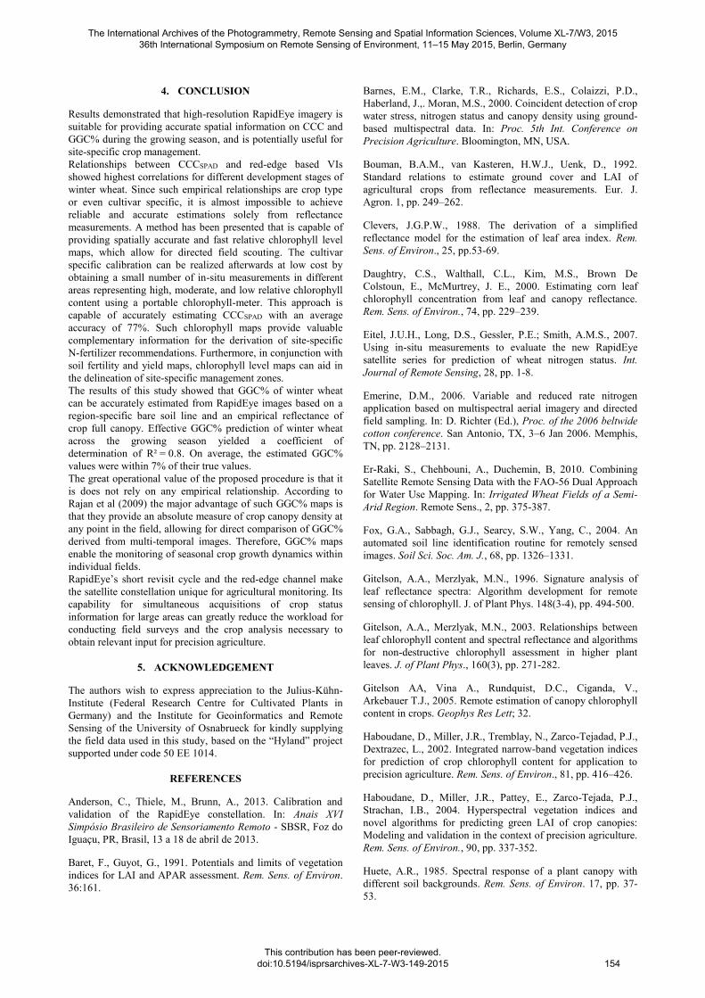
Figure 6 shows the GGC% maps produced for the test field
based on RapidEye images acquired on the 7th of May and 27th
of June 2011. In early May, the GGC% shows considerable
spatial variation in the winter wheat canopy, which might be
suitable for variable rate management. The areas with the
lowest GGC% values correspond to the areas affected by
waterlogging in early spring. In June, the wheat canopy shows
more large-scale variation in GGC% compared to May. The
larger areas with lower GGC% represent areas affected by
drought-stress-induced abnormally premature ripening due to
extreme weather conditions in early summer 2011.
Figure 6. GGC% maps for winter wheat derived from RapidEye
imagery acquired on 7th of May 2011 (top) and on
27th of June 2011 (bottom).
The successful use of a pre-defined, region-specific soil line
and FCP parameters instead of determining them directly from
the image can probably be attributed to the stability of the
sensor calibration over time. Nevertheless, the influence of haze
or other atmospheric effects on the GGC% estimation accuracy
have to be investigated further. In this context, focus has to be
placed especially on the transferability of the empirical full
canopy point reflectance across regions, seasons, and crop
types. Since it is known that VIs show different values for crops
with planophile and erectrophile leaf canopy architecture, the
proposed utilization of an empirical FCP has to be tested on
crops other than winter wheat to help reduce estimation errors.
Y = 0.7691x + 13.483
R² = 0.80
RMSE = 9
The International Archives of the Photogrammetry, Remote Sensing and Spatial Information Sciences, Volume XL-7/W3, 2015 36th International Symposium on Remote Sensing of Environment, 11–15 May 2015, Berlin, Germany
This contribution has been peer-reviewed. doi:10.5194/isprsarchives-XL-7-W3-149-2015
153
4. CONCLUSION
Results demonstrated that high-resolution RapidEye imagery is
suitable for providing accurate spatial information on CCC and
GGC% during the growing season, and is potentially useful for
site-specific crop management.
Relationships between CCCSPAD and red-edge based VIs
showed highest correlations for different development stages of
winter wheat. Since such empirical relationships are crop type
or even cultivar specific, it is almost impossible to achieve
reliable and accurate estimations solely from reflectance
measurements. A method has been presented that is capable of
providing spatially accurate and fast relative chlorophyll level
maps, which allow for directed field scouting. The cultivar
specific calibration can be realized afterwards at low cost by
obtaining a small number of in-situ measurements in different
areas representing high, moderate, and low relative chlorophyll
content using a portable chlorophyll-meter. This approach is
capable of accurately estimating CCCSPAD with an average
accuracy of 77%. Such chlorophyll maps provide valuable
complementary information for the derivation of site-specific
N-fertilizer recommendations. Furthermore, in conjunction with
soil fertility and yield maps, chlorophyll level maps can aid in
the delineation of site-specific management zones.
The results of this study showed that GGC% of winter wheat
can be accurately estimated from RapidEye images based on a
region-specific bare soil line and an empirical reflectance of
crop full canopy. Effective GGC% prediction of winter wheat
across the growing season yielded a coefficient of
determination of R² = 0.8. On average, the estimated GGC%
values were within 7% of their true values.
The great operational value of the proposed procedure is that it
is does not rely on any empirical relationship. According to
Rajan et al (2009) the major advantage of such GGC% maps is
that they provide an absolute measure of crop canopy density at
any point in the field, allowing for direct comparison of GGC%
derived from multi-temporal images. Therefore, GGC% maps
enable the monitoring of seasonal crop growth dynamics within
individual fields.
RapidEye’s short revisit cycle and the red-edge channel make
the satellite constellation unique for agricultural monitoring. Its
capability for simultaneous acquisitions of crop status
information for large areas can greatly reduce the workload for
conducting field surveys and the crop analysis necessary to
obtain relevant input for precision agriculture.
5. ACKNOWLEDGEMENT
The authors wish to express appreciation to the Julius-Kühn-
Institute (Federal Research Centre for Cultivated Plants in
Germany) and the Institute for Geoinformatics and Remote
Sensing of the University of Osnabrueck for kindly supplying
the field data used in this study, based on the “Hyland” project
supported under code 50 EE 1014.
REFERENCES
Anderson, C., Thiele, M., Brunn, A., 2013. Calibration and
validation of the RapidEye constellation. In: Anais XVI
Simpósio Brasileiro de Sensoriamento Remoto - SBSR, Foz do
Iguaçu, PR, Brasil, 13 a 18 de abril de 2013.
Baret, F., Guyot, G., 1991. Potentials and limits of vegetation
indices for LAI and APAR assessment. Rem. Sens. of Environ.
36:161.
Barnes, E.M., Clarke, T.R., Richards, E.S., Colaizzi, P.D.,
Haberland, J.,. Moran, M.S., 2000. Coincident detection of crop
water stress, nitrogen status and canopy density using ground-
based multispectral data. In: Proc. 5th Int. Conference on
Precision Agriculture. Bloomington, MN, USA.
Bouman, B.A.M., van Kasteren, H.W.J., Uenk, D., 1992.
Standard relations to estimate ground cover and LAI of
agricultural crops from reflectance measurements. Eur. J.
Agron. 1, pp. 249–262.
Clevers, J.G.P.W., 1988. The derivation of a simplified
reflectance model for the estimation of leaf area index. Rem.
Sens. of Environ., 25, pp.53-69.
Daughtry, C.S., Walthall, C.L., Kim, M.S., Brown De
Colstoun, E., McMurtrey, J. E., 2000. Estimating corn leaf
chlorophyll concentration from leaf and canopy reflectance.
Rem. Sens. of Environ., 74, pp. 229–239.
Eitel, J.U.H., Long, D.S., Gessler, P.E.; Smith, A.M.S., 2007.
Using in-situ measurements to evaluate the new RapidEye
satellite series for prediction of wheat nitrogen status. Int.
Journal of Remote Sensing, 28, pp. 1-8.
Emerine, D.M., 2006. Variable and reduced rate nitrogen
application based on multispectral aerial imagery and directed
field sampling. In: D. Richter (Ed.), Proc. of the 2006 beltwide
cotton conference. San Antonio, TX, 3–6 Jan 2006. Memphis,
TN, pp. 2128–2131.
Er-Raki, S., Chehbouni, A., Duchemin, B, 2010. Combining
Satellite Remote Sensing Data with the FAO-56 Dual Approach
for Water Use Mapping. In: Irrigated Wheat Fields of a Semi-
Arid Region. Remote Sens., 2, pp. 375-387.
Fox, G.A., Sabbagh, G.J., Searcy, S.W., Yang, C., 2004. An
automated soil line identification routine for remotely sensed
images. Soil Sci. Soc. Am. J., 68, pp. 1326–1331.
Gitelson, A.A., Merzlyak, M.N., 1996. Signature analysis of
leaf reflectance spectra: Algorithm development for remote
sensing of chlorophyll. J. of Plant Phys. 148(3-4), pp. 494-500.
Gitelson, A.A., Merzlyak, M.N., 2003. Relationships between
leaf chlorophyll content and spectral reflectance and algorithms
for non-destructive chlorophyll assessment in higher plant
leaves. J. of Plant Phys., 160(3), pp. 271-282.
Gitelson AA, Vina A., Rundquist, D.C., Ciganda, V.,
Arkebauer T.J., 2005. Remote estimation of canopy chlorophyll
content in crops. Geophys Res Lett; 32.
Haboudane, D., Miller, J.R., Tremblay, N., Zarco-Tejadad, P.J.,
Dextrazec, L., 2002. Integrated narrow-band vegetation indices
for prediction of crop chlorophyll content for application to
precision agriculture. Rem. Sens. of Environ., 81, pp. 416–426.
Haboudane, D., Miller, J.R., Pattey, E., Zarco-Tejada, P.J.,
Strachan, I.B., 2004. Hyperspectral vegetation indices and
novel algorithms for predicting green LAI of crop canopies:
Modeling and validation in the context of precision agriculture.
Rem. Sens. of Environ., 90, pp. 337-352.
Huete, A.R., 1985. Spectral response of a plant canopy with
different soil backgrounds. Rem. Sens. of Environ. 17, pp. 37-
53.
The International Archives of the Photogrammetry, Remote Sensing and Spatial Information Sciences, Volume XL-7/W3, 2015 36th International Symposium on Remote Sensing of Environment, 11–15 May 2015, Berlin, Germany
This contribution has been peer-reviewed. doi:10.5194/isprsarchives-XL-7-W3-149-2015
154
Hunsaker, D.J., Barnes, E.M., Clarke, T.R., Fitzgerald, G.J.,
Pinter, P.J., 2005. Cotton irrigation scheduling using remotely
sensed and FAO-56 basal crop coefficients. American Society
of Agricultural Engineers, St.Joseph, MI.
Jackson, R.D., Pinter, P.J., Paul, J., Reginato, R.J., Robert, J.,
Idso, S.B., 1980. Hand-held radiometry. Agricultural Reviews
and Manuals ARM-W-19. Oakland, California: U.S.
Maas, S.J., Brightbill, J., Hooton, J., 2004. Remote sensing for
precision agriculture in the Texas High Plains. In: P. Dugger,
D. Richter (Eds.), Proc. of the 2004 beltwide cotton
conferences San Antonio, TX, 5–9 Jan 2004. Memphis, TN, pp.
184–187.
Maas, S.J., Rajan, N., 2008. Estimating ground cover of field
crops using medium-resolution multispectral satellite imagery.
Agron. J. 100, pp. 320–327.
Rajan, N., Maas, S.J., 2009. Mapping crop ground cover using
airborne multispectral digital imagery. Precision Agriculture
10(4), pp. 304-318.
Reeves, D.W., Mask, P.L., Wood, C.W., Delano, D.P., 1993.
Determination of Wheat Nitrogen Status with Hand-held
Chlorophyll Meter: Influence of Management Practices, J.
Plant Nutrition, 16, pp. 781–796.
Richardson, A.J., Wiegand, C.L., 1977. Distinguishing
vegetation from soil background information. Photogrammetric
Engineering and Remote Sensing, 43(12), pp. 1541-1552.
Rondeaux, G., Steven, M., Baret, F., 1996. Optimization of Soil
adjusted vegetation indices. Rem. Sens. of Environ., 55, pp. 95-
107.
Rouse, J.W., Haas, R.H., Schell, J.A., Deering, D.W., 1973.
Monitoring vegetation systems in the Great Plains with ERTS,
Third ERTS Symposium, NASA SP-351 I, pp. 309-317.
Scharf, P.C., Lory, J.A., 2002. Calibrating corn color from
aerial photographs to predict sidedress nitrogen need. Contrib.
from the Missouri Agric. Exp. Stn. J. Ser. No.13086. Agron. J.
94, pp. 397–404.
Schulthess, U., Timsina, J., Herrera, J. M., McDonald, A.,
2013. Mapping field-scale yield gaps for maize: An example
from Bangladesh, Field Crops Research, 143(1) pp. 151-156.
Siegmann, B., Jarmer, T., Lilienthal, H., Richter, N., Selige, T.,
Höfle, B., 2013. Comparison of narrow band vegetation indices
and empirical models from hyperspectral remote sensing data
for the assessment of wheat nitrogen concentration. In: Proc.
8th EARSeL SIG IS workshop, Nantes, France.
Xu D, Guo X., 2013. A Study of Soil Line Simulation from
Landsat Images in Mixed Grassland. Remote Sens., 5(9), pp.
4533-4550.
Zhu, J., Tremblay, N., Liang, Y., 2012. Comparing SPAD and
atLEAF values for chlorophyll assessment in crop species,
Canadian J. of Soil Science, 92, pp. 645-648.
The International Archives of the Photogrammetry, Remote Sensing and Spatial Information Sciences, Volume XL-7/W3, 2015 36th International Symposium on Remote Sensing of Environment, 11–15 May 2015, Berlin, Germany
This contribution has been peer-reviewed. doi:10.5194/isprsarchives-XL-7-W3-149-2015
155