cross-asset speculation in stock markets

THE JOURNAL OF FINANCE • VOL. LXIII, NO. 5 • OCTOBER 2008

Cross-Asset Speculation in Stock Markets

DAN BERNHARDT and BART TAUB∗

ABSTRACT

In practice, heterogeneously informed speculators combine private information aboutmultiple stocks with information in prices, taking into account how their trades in-fluence the inferences of other speculators via prices. We show how this speculationcauses prices to be more correlated than asset fundamentals, raising price volatility.The covariance structure of asset fundamentals drives that of prices, while the co-variance structure of liquidity trade drives that of order flows. We characterize howspeculator profits vary with the distributions of information and liquidity trade acrossassets and speculators, and relate the cross-asset factor structure of order flows tothat of returns.

STOCK MARKETS ARE CHARACTERIZED by many stocks and many traders. Specula-tors, especially institutional traders, often interact strategically in many stockssimultaneously. When asset values are correlated, private information aboutone stock may well provide a speculator information about other stocks that hewill incorporate in his trading. For example, a speculator with private informa-tion about a new drug from Merck that affects the value of Glaxo Smith Klinemay trade both stocks.

But strategic interactions are far richer than just this observation suggests.In practice, speculators also observe prices and use that information when trad-ing. Concretely, traders may use information in the price of Glaxo to adjusttrades of Merck. Speculators also understand that their trades convey infor-mation to others via their impacts on prices and that prices reflect informationof other speculators that they, themselves, can use.

The contribution of this paper is to characterize equilibrium outcomes in thissetting. To do so, we first solve for how speculators combine private informationabout different assets with the public information in prices to determine howmuch of each stock to trade. We then derive explicit analytical characteriza-tions of the correlation structure of prices and order flows, determining bothhow are they driven by the correlation structure of asset fundamentals andliquidity trade, and how they are affected by the observability of prices; in ad-dition, we quantify the links between the factor structures of order flows and

∗Bernhardt is with the Departments of Economics and Finance, University of Illinois atUrbana-Champaign. Taub is with the Department of Economics, University of Illinois at Urbana-Champaign. We thank Pete Kyle, Anat Admati, Burton Hollifield, Campbell Harvey (the editor), ananonymous referee, and participants in workshops at the University of Illinois and Simon FraserUniversity for helpful comments. The authors gratefully acknowledge financial support from theNational Science Foundation grant SES-0317700.

2385

2386 The Journal of Finance

prices. Finally, we document numerically how trading strategies and profitsvary with the distributions of information and liquidity trade across assets andspeculators.

The central studies of multi-asset stock markets are Admati (1985) andCaballe and Krishnan (1994). Each of these papers simplifies the strategicsetting along one dimension to obtain answers about other dimensions. Admatidevelops a multi-asset, noisy rational expectations model with a continuum ofagents. Her model has the feature that agents condition trades on both theirprivate signals and stock prices. However, the continuum of agents precludesindividual strategic behaviour—the informationally small agents ignore theprice impact of their trades and do not have to account for how their trades af-fect information release. But, in practice, informed agents for a given stock arefew in number. Those few speculators are typically institutional traders whounderstand that their significant trading has price impacts that they shouldand do anticipate and internalize. To realistically model trading, it is importantto account for such strategic informed trade.

Caballe and Krishnan (1994) develop a static multi-asset formulation of thecompetitive dealership model of Kyle (1985) and Admati and Pfleiderer (1988):Speculators internalize the price impacts of their trades, but do not see prices.Hence, as in Admati (1985), speculators need not worry about the informa-tion their trades convey to other speculators. But, in practice, speculators useinformation in stock prices when trading, and they worry about informationdissemination via prices.

Our model melds these two models, creating a strategic analogue of Admati’snoisy rational expectations equilibrium (REE) model, along the lines of Kyle(1989).1 As in Admati, risk-neutral speculators combine private informationabout various stocks with the information in prices to determine how much ofeach stock to trade. As in Caballe and Krishnan, speculators internalize howtrades influence prices. In dynamic stock markets, speculators use informationin existing prices when determining trades, and strategically account for how,via prices, their trades influence the inferences of other speculators, and hencethe trades of other speculators. Combining observable prices with strategicspeculators lets us capture this key feature of real world markets in a tractablestatic setting. In particular, a speculator in our model must account for how,via prices, his trades influence those of other speculators.

We first derive the form of equilibrium strategies. We prove that strategieshave a forecast error structure: From their direct trades on private signals,

1 There is a large literature on the Kyle (1985, 1989) models of speculation with one asset inone market; see the review by Biais, Glosten, and Spatt (2005). More closely related is the lit-erature on splitting orders for the same asset across multiple markets, initiated by Chowhdryand Nanda (1991) and Dennert (1993), and extended by Bernhardt and Hughson (1997) and Biais,Martimort, and Rochet (2002) to allow for separated, strategic market makers who internalize howtheir pricing influences the division of orders by traders across markets. Other papers considerparameterized multi-asset models in which market makers only see their own order flow and lookat cross-autocorrelations in returns (see Chan (1993), Bernhardt and Mahani (2007), or Chordiaand Swaminathan (2004)).

Cross-Asset Speculation in Stock Markets 2387

traders subtract the projections onto net order flows, so that a speculator’s nettrades correspond to the errors in market maker forecasts of his direct trades.The economics underlying this result is that a speculator’s relevant privateinformation consists of the differences between what his signals are and whatmarket makers perceive those signals to be.

We then prove that there is a unique linear equlibrium. Establishing theexistence of an equilibrium is a formidable task due to the matrix structure in-herent in multi-asset settings. With observable prices and nonstrategic traders,Admati (1985) sets out (p. 633) the technical difficulties that explain why themethods used by Hellwig (1980) to prove existence for a single asset do notextend. Indeed, Admati does not prove existence. Strategic, informationallylarge speculators present further challenges: We must resolve the forecasting-the-forecasts-of-others issues that arise in this multi-asset strategic settingwhen speculators use private information to filter the information in prices(see Townsend (1985), Pearlman and Sargent (2005), or Malinova and Smith(2003)).

To prove existence, we set up an iterative best-response mapping. Given aninitial conjecture about trading strategies—a conjectured matrix of tradingintensities—we compute the associated pricing, and solve for how speculatorsshould filter prices. We then compute best responses by speculators to these con-jectures and iterate, using these best responses as the next conjectures. Whilebest responses are not well behaved, their inner product is, and for this recur-sion we derive conditions under which this mapping is a contraction, whosefixed point corresponds to the equilibrium. This proof is novel and unrelated tostandard contraction mapping constructions in growth theory.2

We go beyond this fundamental analysis to provide new analytical and quan-titative characterizations of the economic structure of both our environmentand that of Caballe and Krishnan. By contrasting equilibrium outcomes whenspeculators can see prices with those when they cannot, we show how the in-formational structure of the market matters.

(1) We derive analytically the correlation structures of order flows andprices. We prove that in our observable price framework, these correla-tion structures are dual in the following sense: The correlation structureof prices is driven only by the correlation structure of asset value funda-mentals, while the correlation structure of order flows is driven only bythe correlation structure of liquidity trade. The economic logic for theseresults is also dual: Were the correlation structure of liquidity tradeto affect that of prices, then prices would be systematically driven byprocesses other than value, and risk-neutral speculators would exploitsuch systematic mispricing; and were the asset value correlation struc-ture to affect that of order flows, then market makers would unravel it,lowering speculator profits.

2 Bernhardt, Taub, and Seiler (2007) analyze a dynamic stationary model with a single stockand provide a related contraction mapping argument on a function space.


(2) We prove that in integrated markets, prices are more correlated thanthe underlying fundamentals, especially when traders see prices. This isbecause in integrated markets, market makers exploit the informationin cross-asset order flows. The resulting high cross-asset correlations inprices raise price volatility.

(3) Outcomes are very different when speculators cannot see prices. Moststarkly, with unobservable prices, symmetrically situated speculators,and uncorrelated liquidity trade, speculators do not trade on cross-assetinformation. For example, a speculator with a signal about Merck’s valuethat is correlated with Glaxo’s value only uses that signal to trade Merck.It is not that the information structure is irrelevant, but the opposite:Speculators trade only on direct signals because order flow for Merckalso affects the price of Glaxo. In contrast, when speculators see prices,they use Merck signals to trade Glaxo because they can subtract fromtheir trades on signals the projections onto prices, reducing the infor-mation that market makers can extract from each order flow, therebymitigating the total price impacts of their trades.

(4) We derive how the factor structure of order flow is related to that ofprices. Hasbrouck and Seppi (2001) apply a principal component de-composition of cross-asset order flows and returns, and find that com-monality in order flows explains roughly two-thirds of the commonalityin returns. We carry out a similar decomposition in our model. We findthat a moderate cross-asset correlation in asset value fundamentals plusa slight positive correlation in liquidity trade across assets can quanti-tatively match their empirical finding.3 The primitive parameters thatwe identify—the correlations in information and liquidity trade—thusprovide a theoretical underpinning to Hasbrouck and Seppi’s purely em-pirical analysis.

We conclude by providing the first quantitative characterizations of equilib-rium outcomes in multi-asset strategic settings for both symmetric and asym-metric environments.

(1) We find that observable prices drive expected speculator profits downsharply, especially when there are more speculators. Underlying thisresult is the information exchange through prices, which induces spec-ulators to trade more aggressively. In particular, each speculator inter-nalizes the fact that as he increases an order, other speculators see theprice impacts and reduce their orders.

(2) We find that the impact of the division of information between specula-tors is very different from the impact of the division of information orliquidity trade across assets. Total speculator profits are very sensitiveto the division of information between speculators, falling sharply wheninformation is more evenly divided and prices are observable. In starkcontrast, divisions of information or liquidity trade across assets have

3 Interestingly, this qualitative result also holds when prices are unobservable.


only second-order effects on total speculator profits. However, this profitirrelevance result masks the complicated ways in which asymmetriesacross assets interact with the market structure to influence how spec-ulators trade, and how equilibrium prices weight order flows in eachmarket. For example, speculators may trade against their cross-assetinformation in a relatively illiquid market.

We next set out the model and analyze a speculator’s optimization problem.In Section II, we then specialize to a symmetric setting to obtain analytical re-sults. Section III offers numerical characterizations, showing how asymmetriesaffect outcomes. A conclusion follows in Section IV. All proofs are given in theAppendix.

I. The Model

In our multi-asset model of speculative trade in a stock market, speculatorsare strategic and internalize how their trades affect prices, and hence the infer-ences and trades of other speculators. N risk-neutral informed speculators andexogenous noise traders trade claims to M assets. Prices are set by risk-neutral,competitive, uninformed market makers.

We denote the vector of asset values by v′ = (v1, . . . , vM). We consider a verygeneral formulation in which asset values are linear functions of K underly-ing fundamentals, e′ = (e1, . . . , eK ). These K fundamentals are jointly normallydistributed with means that we normalize to zero and an arbitrary variance–covariance matrix, �e. The value of asset j is given by

vj = vj 1e1 + vj 2e2 + · · · + vj K eK .

We can write the vector of asset values as v = Ve, where V is the M × K matrix,

v11 v12 · · · v1K

v21 v22 · · · v2K

......

. . ....

vM1 vM2 · · · vM K

.

We allow for the possibility that each speculator has access to many sources ofprivate information about asset values. Specifically, we let speculator i see avector of signals about the value fundamentals, si = Aie, where Ai is an Li × Kmatrix,

si1

si2...

siLi

=

Ai11 Ai

12 · · · Ai1K

Ai21 Ai

22 · · · Ai2K

......

. . ....

AiLi1

AiLi2

· · · AiLi K

e1

e2

...eK

.

Example: One speculator sees an asset’s value. There are M assets, N = M spec-ulators, and K = M fundamentals. The value of asset j is vj = ej, that is, V is


the M × M identity matrix. Only speculator i sees vi = ei, that is, sii = ei and

sij = 0, j = i. The Ai matrix capturing speculator i’s information is an M × M

matrix, which has only zero entries save for Aiii, which is one.

Example: Each speculator receives one signal for each asset. There are Massets, N speculators, and K = MN fundamentals. The value of asset j isvj = e(j−1)N+1 + · · · + e(j−1)N+i + · · · + ejN . Thus, V is an M × MN matrix, wherethe jth row of V captures the value of asset j, so it has vj,(j−1)N+i = 1 fori = 1, . . . , N, and zeros elsewhere. Speculator i sees si

j = e(j−1)N+i for assetj = 1, . . . M. Then Ai is an M × MN matrix, where the j th row of the Ai ma-trix captures speculator i’s information about asset j: It has Ai

j,(j−1)N+i = 1, andzeros elsewhere.

In addition to his signals si, speculator i knows the prices at which orders foreach asset will be executed. That is, our economy is a noisy rational expectationseconomy in which agents are strategic and internalize how their trades affectprices and the information content of prices. It is in this sense that our modelextends and melds the models of Admati (1985) and Caballe and Krishnan(1994), allowing us to capture key aspects of a dynamic market in a simplerstatic setting.

Let xij be speculator i’s order for asset j, let xi′ = (xi

1, xi2, . . . , xi

M ) be the vector

of his orders, and let X ′ = (X 1, X 2, . . . , X M )′ = (∑N

i=1 xi1,

∑Ni=1 xi

2, . . . ,∑N

i=1 xiM )

be the vector of net order flows across assets from speculators. In additionto trade from speculators, there is exogenous liquidity trade of asset j of uj.We let u′ = (u1, u2, . . . , uM) be the vector of liquidity trades. Liquidity trade isdistributed independently of the value fundamentals, and hence of speculatorsignals. We allow for a general correlation structure in liquidity trade acrossassets, assuming only that liquidity trade is jointly normally distributed withzero mean and variance–covariance matrix �u.

Markets are cleared by competitive market makers who use the trading ac-tivity throughout the entire stock market when setting prices. In particular,a market maker observes the net order flow for his asset, and the prices ofother assets. Equivalently, with linear pricing, market makers see the vector ofnet order flows for all assets, (X + u)′ = (X1 + u1, X2 + u2, . . . Xm + um). Marketmakers set the price of each asset equal to its expected value given the vector ofnet order flows, that is, pj = E[vj|(X + u)′]: Competition drives market makerexpected profits from filling each order down to zero. At the period’s end, assetsare liquidated and trading profits are realized.

We focus on equilibria in which speculators adopt trading strategies thatare linear functions of both their private signals and net order flows, andmarket makers set prices that are linear functions of net order flows.Specifically, we conjecture that speculator i’s order for asset j takes theform

xij = bi

j 1si1 + bi

j 2si2 + · · · + bi

j Lisi

j Li+ Bi

j 1(X 1 + u1) + Bij 2(X 2 + u2)

+ · · · + Bij M (X M + uM ).


Hence, the vector of speculator i’s orders is xi = bisi + Bi(X + u), that is,

xi1

xi2...

xiM

=

bi11 bi

12 · · · bi1Li

bi21 bi

22 · · · bi2Li

......

. . ....

biM1 bi

M2 · · · biM Li

s1

s2

...sLi

+

Bi11 Bi

12 · · · Bi1M

Bi21 Bi

22 · · · Bi2M

......

. . ....

BiM1 Bi

M2 · · · BiM M

X 1 + u1

X 2 + u2

...X M + uM

.

Thus, bi represents i’s trading intensities on his signals, and Bi represents i’strading intensities on the net order flows that he sees. The conjecture thatpricing is a linear function of net order flows implies that p = λ(X + u), wherethe pricing matrix λ is an M × M invertible matrix that aggregates informationfrom the order flows of all assets to determine prices, that is,

p1

p2

...pM

=

λ11 λ12 · · · λ1M

λ21 λ22 · · · λ2M

......

. . ....

λM1 λM2 · · · λM M

X 1 + u1

X 2 + u2

...X M + uM

.

The extent to which a market maker uses information from other stocks toprice a particular stock, and not just a stock’s own order flow, is captured by thenondiagonal elements of λ. Because the pricing matrix λ is invertible, observingprices is equivalent to observing net order flows.

Equilibrium. In a linear equilibrium, speculators maximize expected tradingprofits given correct conjectures, net order flows are consistent with speculatoroptimization, and market makers earn zero expected profits from filling eachorder given the vector of net order flows.

Speculator’s Optimization Problem. Speculator i seeks to maximize ex-pected trading profits given his signals si and the net order flows X + u,solving

maxxi

E[(v − p)′ xi|si, X + u] = maxxi

E

[(v − λ

(N∑

k=1

xk + u

))′xi|si, X + u

]. (1)

To solve for speculator i’s best response to the conjectured linear trading strate-gies of the other speculators and the linear pricing, we first rewrite the vector


of net order flows from i’s perspective,

X + u = xi +∑k =i

(bksk + Bk(X + u)) + u. (2)

Defining qi ≡ (I − ∑k =i Bk)−1, we solve equation (2) for

X + u = qi

(xi +

∑k =i

bksk + u

). (3)

Speculator i understands and internalizes how his orders affect the trades ofother speculators through price via qi. Substituting for X + u into speculatori’s objective yields

maxxi

E

[(v − λqi

(xi +

∑k =i

bksk + u

))′xi|si, X + u

]. (4)

The associated first-order condition with respect to xi is

0 = E[(v − λ(X + u))′ − qi′λ′xi|si, X + u]. (5)

Proposition 1 describes the forecast error structure of a speculator’sorders.

PROPOSITION 1: Speculator i’s vector of orders, xi, is a linear function of theforecast errors of his trades on his private signals.

Proposition 1 reflects that a speculator’s relevant private information con-sists of the differences between what his signals si are, and what the mar-ket maker perceives them to be—that is, the errors in the market maker’sforecasts of his signals, si − E[si|X + u]. Accordingly, the vector of speculatori’s net orders, xi, is a linear function of these forecast errors. That is, Bi is amatrix of projection coefficients of trading intensities on private signals ontonet order flows: From their direct trades on private signals, traders subtractthe projections of these trades onto net order flows, so that a speculator’s nettrades correspond to the market maker’s forecast error of his trades on hissignals.

Substituting this forecast error structure, we drop the conditioning on X + ufrom the speculator’s first-order conditions and express the first-order condi-tions solely in terms of the fundamentals. To do so, we first solve for net orderflows in terms of trading intensities on fundamentals:

X + u =N∑

k=1

bksk +N∑

k=1

Bk(X + u) + u

⇒ X + u =(

I −N∑

k=1

Bk

)−1( N∑k=1

bksk + u

).


We then substitute this solution for X + u into speculator i’s trade on net orderflow,

Bi(X + u) = Bi

(I −

N∑k=1

Bk

)−1( N∑k=1

bksk + u

),

and defining γ i ≡ Bi(I − ∑k Bk)−1, we write speculator i’s vector of trades as

xi = bisi + γ i

(N∑

k=1

bksk + u

). (6)

We next add across traders, and defining � ≡ I + ∑k γ k ,we write the vector of

net order flows as

X + u =(

I +N∑

k=1

γ k

)(N∑

k=1

bksk + u

)= �

(N∑

k=1

bksk + u

). (7)

Lemma 1 exploits this structure to write i’s first-order conditions solely asfunctions of γ i and �.

LEMMA 1: The first-order condition characterizing speculator i’s orders is givenby

0 = E

[(I + γ i ′)v − (I + γ i ′)λ�

N∑k=1

bksk − �′λ′(

bisi + γ iN∑

k=1

bksk

) ∣∣∣∣∣si

]. (8)

The crucial point to note in this first-order condition is that the “same” bi

sets the expectation to zero for each si. As a result, we can integrate out oversi: The bi that maximizes expected trading profits given any si also maximizesexpected profits unconditionally. The unconditional maximization problem iseasier to solve because it exploits the fact that the same bi works for everysi.

A. The Unconditional Problem

Informed speculator i’s trading intensities maximize unconditional expectedtrading profits, solving

maxbi ,Bi

E

[(V e − λ�

(N∑

k=1

bk Ake + u

))′(bi Aie + γ i

(N∑

k=1

bk Ake + u

))],

where we recall that v = Ve and si = Aie. Turning to the market maker’s ob-jective, competition drives expected market maker profit to zero. This im-plies that pricing minimizes the variance of the forecast error between pricesand values—prices equal the projection of the vector of equity values onto


net order flows. Hence, pricing solves the following least-squares predictionproblem:

minλ

E

[(V e − λ�

(N∑

k=1

bk Ake + u

))′(V e − λ�

(N∑

k=1

bk Ake + u

))].

Proposition 2 details the first-order conditions for bi, γ i, and λ. To ease presen-tation, we define

bA ≡ (b1 . . . bN )

A1

...AN

.

It also helps to take the portion of net order flow∑N

k=1 bksk + u that excludesorder flow due to the speculators’ filtering of prices, and to define � as the innerproduct of this signal-based order flow,

� ≡ (bA I )(

�e 00 �u

)(A′b′

I

)= bA�e A′b′ + �u. (9)

PROPOSITION 2:

bi : Ai�e A′b′�′λ′(I + γ i) + Ai�e(Ai′bi′ + A′b′γ i′

)λ� = Ai�eV ′(I + γ i) (10)

γ i : γ i ′ = −�−1bA�e Ai ′bi ′ (11)

λ : �′λ′ = �−1bA�eV ′. (12)

The first-order condition for bi, equation (10), characterizes the weightsthat speculator i places on each private signal for each of his trades. Theequation lacks multiplicative symmetry because of the cross-correlation of in-formation. Because of this structure, equation (10) alone cannot be solveddirectly; the array of first-order conditions across all speculators must beconstructed.

The matrix equation (11) for γ i′ is the matrix of regression coefficients ofthe projections of speculator i’s orders based on private signals onto the vec-tor of total net order flows. This equation captures the strategic interactionsbetween speculators via price. The negative sign indicates that speculatorssubtract these projections from their trades on private signals to avoid payinga quadratic cost on the portions of their trades on signals that are revealedthrough prices.

The pricing matrix equation (12) is the matrix of regression coefficients fromthe projection of the vector of values onto the vector of total net order flows. Inequilibrium, market makers have correct conjectures about {γ k}, that is, how


speculators trade on net order flows. Inspecting the pricing equation revealsthat the “effective” pricing filter for market makers, µ ≡ λ� = λ(I + ∑

k γ k), de-pends only on the “primitive” b trading intensities for speculators: Market mak-ers see the same net order flow as speculators, and hence can unwind the {γ k}filtering by speculators to filter directly the signal-based portion,

∑Nk=1 bksk + u.

It follows that the observability of prices ultimately affects profits only throughits effect on the strategic behavior of speculators.

Finally, note that bi and γ i enter nonquadratically into speculator i’s ob-jective. However, the speculator’s objective can still implicitly be decomposedinto two quadratic parts, one in bi and the other in γ i. This is because γ i isthe projection of bisi onto the vector of net order flows and (from Proposi-tion 1) speculator i’s vector of orders is orthogonal to the vector of net orderflows. Even so, the associated first-order conditions characterizing optimiza-tion are nonlinear because the {bk} enter {γ k}, which, in turn, multiply the{bk}. This reflects the strategic use by traders of the information in prices.The practical consequence is that we cannot just invert a matrix to solve forequilibrium trading strategies. Rather, we must iterate, first solving for thebest responses to conjectured trading strategies and pricing, and then iter-atively substituting these best responses in as the basis for a new round ofconjectures.

Stacking the first-order conditions for b′, we can write the recursion as

(a�e A′)b′ =

∑k =1 A1�e Ak′

bk′µ(µ′(I + γ 1) + (I + γ 1′

)µ)−1

...∑k =N AN�e Ak′

bk′µ(µ′(I + γ N ) + (I + γ N ′

)µ)−1

+

A1�eV ′(I + γ 1)(µ′(I + γ 1) + (I + γ 1′)µ)−1

...AN �eV ′(I + γ N )(µ′(I + γ N ) + (I + γ N ′

)µ)−1

.

(13)

The left-hand side represents the vector of best-responses by speculators toconjectured strategies of other speculators and the associated pricing. The con-jectured b′ shows up on the right-hand side both directly and in the {γ k} pro-jections. That is, a conjectured b′ implies values of {γ k} and hence λ� on theright-hand side; and the left-hand side is the best-response to those conjectures.We use an iterative algorithm to solve for the equilibrium values of b. We firstconjecture a value of b′, use this value to compute {γ k} and µ, and then sub-stitute these values into the right-hand side of (13). We then compute the bestresponse to these conjectures. Finally, we use this vector of best responses asthe new vector of conjectured strategies, and iterate.

II. Theoretical Characterizations under Symmetry

The theoretical analysis is more complicated than the discussion above sug-gests. The iterative mapping might not be stable: Each speculator responds to


an entire matrix of trading intensities, and also to a pricing matrix. Becausehis response influences the pricing matrix, a speculator’s best response mightbe to overreact to the trading intensities of rivals. Iteration on this overreac-tion would vitiate the equilibrium. We now demonstrate that the iterated bestresponses are in fact stable. Specifically, we prove in symmetric settings thatfor sufficiently small correlations in asset values, this best-response mappingis a contraction on the appropriate space of matrices. Further, our numeri-cal analysis strongly suggests that the contraction mapping property extendsto asymmetric settings and arbitrary cross-asset correlations. It follows thatthere is a unique linear equilibrium. We present the contraction mapping the-orem in the two-asset, two-speculator setting that we focus on numerically, inwhich each speculator sees one of the two innovations to each asset, and the in-novation that he sees for one asset has correlation θ with the innovation to theother asset that he does not see. The proof considers a more general symmetriccase,4 and the analytical argument extends to environments that are “close” tosymmetric, due to the slackness in the approximation bounds that we derive.We state the simpler case because it lets us simplify presentation by redefiningnotation:

PROPOSITION 3: Let there be two assets, j = 1, 2, and two speculators, i = 1, 2.The value of asset j is vj = e1

j + e2j , for j = 1, 2. Speculator i sees innovations ei

1and ei

2, i = 1, 2, where e1j and e2

j are identically and independently distributed ac-cording to a normal N(0, 1) distribution, and corr(e j

1 , ei2) = θ ≤ 1

3 , for i = j. Letliquidity trade be distributed according to an arbitrary symmetric variance–covariance matrix, �u. Then the mapping T implicit in equation (13) is a con-traction mapping, implying that there is a unique symmetric linear equilibrium.

The proof approach is novel. Because γ i and µ are highly nonlinear in b, thedirect recursion is highly nonlinear. To prove the contraction mapping property,one must transform the direct recursion in b into a recursion of a quadratic formin b, that is, bA�eA′b′. With symmetry, b1 = b2, and we write the recursion inbi(1 θ

θ 1)bi ′ ≡ bi(I + p)bi′ ≡ Q , which is well behaved:

Q = Q(I + p)−1 p(I + γ i)−1 + 1N

�u. (14)

Using (14), we establish the contraction property by showing that the norm ofthe coefficient term (I + p)−1p(I + γ i)−1 is a fraction. The norm of the factor (I +p)−1p can be made arbitrarily small by shrinking θ . Even though (I + γ i)−1 isendogenous, a lemma establishes that its norm is bounded. With the contractionproperty established, we recover the fixed point of bi by finding the Choleskyfactor of the fixed point of the mapping, and then multiplying that factor by the

4 The analysis also applies to the symmetric N-asset, N-speculator environment set out in ex-ample 1, in which speculator i alone sees the sole innovation to asset i.


inverse of the Cholesky factor of I + p, that is, by multiplying by

(1 θ

0 (1 − θ2)12

)−1

.

Unobservable prices. This theoretical analysis also provides an easy way toderive equilibrium outcomes if speculators cannot see prices. With unobservableprices, we obtain equilibrium trading intensities by setting γ i = 0 for all i. Insymmetric settings such as Proposition 3, this allows us to extend Caballe andKrishnan to obtain closed-form solutions: Substituting γ i = 0 into (14) yields

Q = Q(I + p)−1 p + 1N

�u.

Rearranging and substituting back for Q yields

bi(I + p)bi′(I − (I + p)−1 p) = 1

N�u.

Expanding the left-hand side yields

bi(I + p)bi′(I − (I + p)−1 p) = bi(I + p)bi′

(I + p)−1(I + p − p)

= bi(I + p)bi′(I + p)−1 = bibi′

.

Hence, bibi′ = 1N �u. When liquidity trade is uncorrelated across assets, the fol-

lowing is immediate.

COROLLARY 1: If speculators do not see prices, then in symmetric settings inwhich liquidity trade is uncorrelated across assets, speculators only trade di-rectly on their signals—b is a diagonal matrix with identical entries σu√

N.

Concretely, Corollary 1 says that in symmetric settings where speculators donot see prices, each speculator uses his Merck signal only to trade Merck in-dependently of the correlation of the Merck signal with the value of Glaxo.This remarkable outcome arises because speculators understand that a mar-ket maker for Merck will use order flow for Glaxo to price Merck, estimatingthe value of Merck via a projection onto the order flows for both stocks.

In contrast, when speculators see prices, they can account for the marketmaker’s projections. The γ ’s in trading strategies are (minus) the coefficients ofthe projections of the speculators’ direct trades onto order flows (equivalently,prices). Speculators subtract these projections, so that their total net trades areeffectively the market makers’ forecast errors of their direct trades on signals.Hence, the same direct trading intensities convey less information to marketmakers, mitigating the total price impacts of their trades. In turn, this encour-ages speculators to trade more aggressively on the remaining forecast errorcomponents of private information. In particular, in contrast to the unobserv-able price setting, when asset values are positively correlated, a positive signalfor Merck will lead a speculator to buy both Merck and Glaxo.


Extending Corollary 1, we will show numerically that when information orliquidity trade is divided asymmetrically between assets, and speculators donot see prices, then speculators trade against their signal from the more liquidor more volatile stock. For example, when speculators do not see prices, andone asset has more than half of the liquidity trade, speculators trade againstsignals about the more liquid stock in the less liquid market: The direct tradinglosses are more than offset by the beneficial price impact on the more liquidstock. In symmetric settings these two effects have offsetting impacts on prof-its, so that speculators only use “Merck” signals to trade Merck. So, too, withunobservable prices, if one speculator has access to more private informationthan other speculators, the speculator with more information trades against his“cross-asset signal,” selling Merck when he has a positive signal about Glaxo(and asset values are positively correlated). In the observable price setting,asymmetries have similar qualitative marginal effects on cross-asset tradingintensities. However, because speculators can exploit the observability of pricesto subtract the projections of their direct trades, the asymmetries must be ex-treme in order to induce a speculator to trade against cross-asset signals. Forexample, (ceteris paribus) there must be far less liquidity trade in the Merckmarket than the Glaxo market for a speculator to sell Merck when he receivesa positive signal about Glaxo (about 1/8th as much as in our numerical exam-ples). These observations emphasize how radically the observability of pricesalters trading strategies.

A. Trading Strategies

We say that an environment is fully symmetric if information is symmetricallydistributed across both assets and speculators, and liquidity trade is symmet-rically distributed across assets. With this added structure, we now show thattrading strategies take a form that mirrors their structure in standard single-asset settings: Trading strategies are proportional to the ratio of the standarddeviation of liquidity trade to the standard deviation of speculator signals (see,for example, Kyle (1985)).

PROPOSITION 4: In the fully symmetric, two-speculator observable price environ-ment of Proposition 3, speculative trading intensities on intrinsic informationare characterized by

b ∼ (A�e A′)−1/2�1/2u .

In sharp contrast, with unobservable prices, Corollary 1 immediately revealsthat trading strategies are not proportional to (A�eA′)−1/2.

B. Cross-asset Correlations

We now derive a result of the unraveling by market makers of the filteringby traders of order flow.


PROPOSITION 5: In the fully symmetric, two-speculator observable price envi-ronment of Proposition 3, the covariance matrix of price changes, λ��′λ′, isindependent of �u, that is, of the distributional properties of liquidity trade.Only the variance–covariance structure of the innovations to asset values, �e,affects the correlation structure of price changes.

The economic force driving this result is that if the correlation structure ofnoise trade affected the correlation structure of prices, then prices would besystematically driven by processes other than value—market makers wouldbe systematically mispricing stocks—and speculators would exploit this. For-mally, using b ∼ �

1/2u , we have that the inner product of net order flow,

� = bA�eA′b′ + �u ∼ �u; and λ ∼ �−1/2u unwinds the correlation structure of

liquidity trade, leaving only the impact of the variance–covariance struc-ture of intrinsic information. Our numerical investigations indicate thatthis result extends to arbitrary numbers of speculators and to asymmetricsettings.

We next prove that in fully symmetric environments, the strategic behaviorby speculators causes price changes to be more correlated than the underlyingfundamentals. Our numerical investigations strongly suggest that this resultextends more generally to asymmetric environments.

PROPOSITION 6: In the fully symmetric, two-speculator observable price envi-ronment of Proposition 3, price changes (returns) are more correlated than theunderlying fundamentals. For small correlations in fundamentals, θ , the pricechange correlation is approximately 5

3θ .

Corollary 1 revealed that in symmetric settings, unobservable prices causespeculators to trade only on their direct signals; whereas with observable prices,speculators weight positively their signal for one asset when trading the otherasset. Proposition 6 just showed that observable prices cause price changes tobe more correlated than the underlying fundamentals; and we find numericallythat price changes are more correlated when prices are observable than whenthey are not. These findings would seem to suggest that the cross-asset cor-relations in net order flow should be higher when speculators see prices thanwhen they do not. We now show that this intuition is completely misplaced.The variance–covariance matrix of net order flows is �(bA�eA′b′ + �u)�′. Thenext result shows that this matrix takes a simple form.

PROPOSITION 7: The variance–covariance matrix of net order flows is �u�′. In thefully symmetric, two-speculator observable price environment of Proposition 3,only the variance–covariance structure of liquidity trade, and not the correlationstructure of the innovations to asset values, �e, affects the correlation structureof order flows.

Numerical analysis suggests that this result extends more generally to asym-metric environments. The economic force driving this result is analogous tothat for the correlation structure of pricing—were net order flows to reflect the


correlation structure of speculators’ private information, market makers wouldexploit this in their pricing, reducing speculator profits. The upshot of Propo-sitions 5 and 7 is that the correlation structures of order flow and prices aredual to each other in the following sense: The covariance structure of prices isdriven only by the covariance structure of value, while the covariance structureof order flows is driven only by the covariance structure of liquidity trade.

The next proposition derives the surprising consequences of Proposition 7 forthe correlation structure of net order flows when liquidity trade is uncorrelatedso that only the intrinsic correlation in fundamentals and strategic speculativebehavior affect the order flow correlation.

PROPOSITION 8: Consider the fully symmetric, two-speculator environment ofProposition 3, and suppose that liquidity trade is uncorrelated across assetsand asset values are positively correlated, that is, θ > 0. Then, with observableprices, cross-asset net order flows are negatively correlated. If, instead, prices areunobservable, cross-asset net order flows are positively correlated.

With observable prices, the negative correlation in cross-asset net order flowsis immediate: With uncorrelated liquidity trade, �u is diagonal, so the cross-asset correlation takes the sign of the off-diagonal term in � = �′, γij, which isnegative. Even though speculators trade directly on their cross-asset signals,they also subtract out the projections of these direct trades onto net order flows,and with uncorrelated liquidity trade this latter effect dominates, leading tonegative cross-correlations in net order flows.

In contrast, with unobservable prices, speculator 1’s signal for asset 1 is cor-related with speculator 2’s signal for asset 2, and both trade with the sameintensity on those signals. As a result, even though speculators only trade ondirect signals, the cross-asset correlation in order flow is positive. Hence, withuncorrelated liquidity trade, observable and unobservable prices generate op-posing predictions—but they are the opposite of what a casual contemplation ofdirect cross-asset trading intensities suggests. This result indicates that withobservable prices, some correlation in liquidity trade is needed to reconcile thepositive cross-asset correlation in order flows found in the data.

Numerical investigation reveals that with observable prices and modest cor-relation in liquidity trade across assets (relative to the correlation in privatesignals), net order flows become positively correlated across assets, but remainless correlated than liquidity trade. In contrast, with unobservable prices, netorder flows are always more correlated than liquidity trade.

C. Factor Structure

Hasbrouck and Seppi (2001) apply a principal component decomposition ofcross-asset order flows and returns, and find that commonality in order flowsexplains roughly two-thirds of the commonality in returns. We can apply thesame decomposition in our model to cross-asset order flows and price changes(our analogue of returns). This factor analysis reveals the dimensions along


which our stylized model can reconcile the data. Moreover, the primitive pa-rameters that we generate—the correlation in information of speculators andthe correlation in liquidity trade—provide a theoretical underpinning for Has-brouck and Seppi’s purely empirical findings.

Hasbrouck and Seppi note that the principal common factors of cross-assetorder flow and cross-asset returns are the eigenvectors of the covariance matrixof the relevant variable. The eigenvectors are ordered by the magnitudes ofthe corresponding eigenvalues. Hasbrouck and Seppi initially regress returnson the first principal component of order flow PX+u. This results in a set ofresiduals wt. They next calculate the principal components of those residuals,Pw. Finally, they show that together PX+u and Pw explain 21.7% of the totalvariance of returns, of which PX+u comprises 14.6%, or about two-thirds.

We can carry out a parallel principal components analysis in our model. Toease presentation, we focus on a two-asset, two-speculator, fully symmetric set-ting. With symmetry, the covariance matrices of order flow and price changestake the form (a b

b a). The associated eigenvalues are a − b and a + b, and eigen-vectors are 2−1/2(−1

1 ) and 2−1/2(11). The scaling factor 2−1/2 can be ignored as itdrops out in the calculations. We focus on the empirically relevant case where(a) cross-asset order flows and (b) cross-asset returns (price changes) are eachpositively correlated. With positive correlation, a + b is the larger eigenvalueand (11) is the corresponding eigenvector.

The analogue of Hasbrouck and Seppi’s first-step regression analysis in ourmodel is

pi = cP X +u + wi,

where c is a regression coefficient and wi is a residual. Exploiting symmetry,we have

c = cov(pi, q1 + q2)var(q1 + q2)

= cov(λi1q1 + λi2q2, q1 + q2)var(q1 + q2)

= λi2 + λi1

2.

The covariance matrix of the residuals is

cov(

w1

w2

)= cov

(p1 − cP X +u

p2 − cP X +u

)= cov

(p1 − c(q1 + q2)p2 − c(q1 + q2)

).

Under symmetry, the eigenvalues again take the form a − b and a + b. Therelevant principal component is

w1 − w2 = p1 − c(q1 + q2) − (p2 − c(q1 + q2)) = q1 − q2,

as it must be orthogonal to PX+u.5

Following Hasbrouck and Seppi, we next calculate the regression coefficientsfor wi on Pw:

wi = di Pw + εi.

5 The other principal component is (1 − 2c)(q1 + q2), which is perfectly correlated with PX+u.


With the principal component (q1 − q2), we obviously have d2 = −d1, where

d1 = cov(p1 − c(q1 + q2), q1 − q2)var(q1 − q2)

= cov((λ11 − c)q1 + (λ12 − c)q2, q1 − q2)var(q1 − q2)

.

Substituting for λ11 − c = λ11 − λ12

2and λ12 − c = λ12 − λ11

2, and rearranging

yields

d1 =cov

(λ11 − λ12

2(q1 − q2), q1 − q2

)var(q1 − q2)

= λ11 − λ12

2.

The respective shares of the total variation attributed to PX+u and Pw are

S(P X +u) = 2c2 var(P X +u)var(p1) + var(p2)

= 2c2 var(q1 + q2)var(p1) + var(p2)

= 2c2 var(qi) + cov(q1, q2)(λ2

ii + λ2i j

)var(qi) + 2λiiλi j cov(qi, qj )

S(Pw) = 2d2i

var(Pw)var(p1) + var(p2)

= 2d2i

var(q1 − q2)var(p1) + var(p2)

= 2d2i

var(qi) − cov(q1, q2)(λ2

ii + λ2i j

)var(qi) + 2λiiλi j cov(qi, qj )

,

which we can calculate numerically.Calibration. Our model is sufficiently stylized that it is not directly compa-rable to the Hasbrouck and Seppi framework. To appreciate the stylization,note that in our model only two factors drive pricing (reflecting the two netorder flows),6 whereas Hasbrouck and Seppi find three significant factors.Further, in our two-asset model, the ratio of the first two eigenvalues is en-tirely driven by the correlation structure of the matrices, whereas in the data,the correlation structure is not the sole determinant. We also consider a sym-metric setting, whereas Hasbrouck and Seppi average over heterogeneousstocks.

Our findings in Propositions 4 and 5 that (a) speculative trade is proportionalto (A�eA′)−1/2�

1/2u and (b) the correlation of price changes is unaffected by the

cross-asset correlation of liquidity trade η together imply that as long as thecorrelation in liquidity trade is high enough that cross-asset order flows arepositively correlated, then S(P X +u)

S(P X +u)+S(Pw) depends only on the cross-asset signalcorrelation θ , and not on either η or the scales of asset value innovations andliquidity trade. Raising θ increases the fraction explained by commonality inorder flow. We find that a relatively small signal correlation of θ = 0.2 generates

6 We would have more factors if we added noise from public information arrival or order flowfrom additional heterogeneous assets.


the two-thirds share ratio that Hasbrouck and Seppi find.7 For θ = 0.2, thecross-asset correlation in liquidity trade must be at least η = 0.135 for net orderflows to be positively correlated (and, for example, η = 0.25 generates a netorder flow correlation of 0.12).

Taking our model further, we can compare the ratios of the first two eigen-values in the covariance matrices of order flow and price changes with theirempirical counterparts. Fixing θ = 0.2, a liquidity trade correlation of η = 0.5allows us to match the 2.183 eigenvalue ratio for order flows that Hasbrouckand Seppi find. Because the correlation of price changes is unaffected by thecorrelation of liquidity trade, η only influences the eigenvalue ratio for or-der flow; and θ = 0.2 implies an eigenvalue ratio for price changes of 1.968,which is about one-third of the ratio for returns that Hasbrouck and Seppifind.

Summarizing, we highlight three points. First, our model can generate the re-sult that the primary principal factor for order flow is also the main influence onprice changes or returns. This result requires a relatively small and believablecross-asset correlation in innovations to asset values. Second, we require someminimal level of cross-asset correlation in liquidity trade,8 and a relatively highcorrelation in liquidity trade to match the eigenvalue ratio that Hasbrouck andSeppi find. Third, with unobservable prices, one needs a slightly higher corre-lation in value innovations, θ = 0.236, to match S(P X +u)

S(P X +u)+S(Pw) = 2/3; η = 0.283allows us to match the eigenvalue ratio for order flow; and θ = 0.236 impliesan eigenvalue ratio for price changes of 2.071.

III. Numerical Characterizations

We now explore the quantitative properties of our model further. To isolatethe strategic effects due to information linkages across assets, we normalizeparameter values so that if (a) a market maker only sees the net order flowfor his own stock and (b) speculators do not see prices, then (c) total expectedspeculator profits do not change as we vary the parameters that describe theeconomy. It follows that any variations in speculator profits in an integratedstock market are due to the interaction between the economic environment andmarket information structure.

If speculators only see their private signals and do not see prices, and amarket maker only sees the net order flow for his stock, it is well known (Kyle(1985)) that trading strategies for each asset are proportional to the ratio ofthe standard deviation of liquidity trade to the standard deviation of informed

7 In our model, S(P X+u) + S(P w) = 1 because our model has no noise, so that the order flowsof the two assets perfectly determine pricing—simply adding a third heterogeneous asset wouldchange this.

8 This should not be confused with standard “measures” of liquidity—the inverses of the esti-mated λii—which are constants in our model, reflecting the amounts of intrinsic private informa-tion relative to liquidity trade. In our model, correlation of liquidity trade is reflected in the useby market makers of cross-asset order flow in pricing—that is, the off-diagonal elements of the λ

matrix.


signals, σuσe

. Hence, pricing is proportional to σeσu

, and expected speculator profitsare proportional to σuσe. Therefore, multiplying the variance–covariance matrixof signals by a constant simply scales trading intensities and profits, so wecan normalize these totals without loss of generality; the variance–covariancematrix of liquidity trade can be normalized for the same reason.

We perturb the economy in three ways.Division of Information between Speculators. We impose symmetry across assetvalues and liquidity trade, and vary the share of the variance to asset valuesthat one speculator observes. This isolates how the division of private informa-tion between speculators affects equilibrium outcomes. The normalization thatpreserves total expected speculator profits when a market maker only observesown order flow holds constant the total variance of each asset and preservesthe cross-asset value correlation structure. Within this setting, we characterizethe impact of increased competition by varying the number of speculators whoreceive the same set of signals.Division of Liquidity Trade between Assets. We impose symmetry across assetvalues and speculator signals, and vary the share of liquidity trade betweenassets. This isolates the effects of relative liquidity levels between assets. Withindependently distributed liquidity trade, the appropriate normalization holdsconstant the sum of the standard deviations of liquidity trade across assets.Division of Uncertainty between Assets. We impose symmetry across speculatorsand liquidity trade and vary the variance share of asset values between assets.This isolates the effects of relative levels of private information between assetson equilibrium outcomes. The normalization holds constant the sum of thestandard deviations of asset values and preserves the correlation structure.

A. Division of Information between Speculators

Our numerical analysis focuses on the economic environment of Example 2,in which speculators see one signal for each asset. In our base two-speculator,two-asset setting, liquidity trade is independently and normally distributedwith ui ∼ N(0, 1). Using the notation of Proposition 3, the value of asset j isvj = e1

j + e2j . Speculator i sees signal si

1 = ei1 for asset 1 and signal si

2 = ei2 for

asset 2. The signals e1j and e2

j that the two speculators receive for asset j areindependently and normally distributed with mean zero. However, even thoughspeculator 1 does not see e2

1, we allow cross-asset signal correlations to be posi-tive, corr(ej

1, ei2) = θ , for i = j, so that speculator 1’s signal e1

2 about asset 2 alsoprovides him information about the innovation e2

1 to asset 1 that he does notsee. The variance–covariance matrix for asset value innovations is

e11 e2

1 e12 e2

2

e11

e21

e12

e22

ν 0 0 θξ

0 (1 − ν) θξ 00 θξ ν 0θξ 0 0 (1 − ν)

,


where ξ = √ν(1 − ν) is the normalization factor that preserves the correlation

structure as we vary the information that speculator 1 has relative to speculator2. We vary ν from 0.1 (so that speculator 1 sees 10% of the variance of each assetvalue) to ν = 0.9. Because of the cross-asset correlation structure, speculator1’s share of the private information is

var(e1

1

) + var(E

[e2

1|e12

] )var

(e1

1

) + var(E

[e2

1|e12

] ) + var(E

[e1

1|e22

] ) + var(e2

1

) = ν + θ2(1 − ν)1 + θ2

.

We focus on a high correlation of θ = 0.75, as higher correlations largely serveto magnify the qualitative impacts.9

The top line in Figure 1 represents expected total speculator profits whenmarket makers only see “own” net order flow and speculators do not see prices.Their constancy reflects that we have normalized informational parameters toleave profits in this setting unaffected by the division of information betweenspeculators. The middle line plots profits in the Caballe–Krishnan environmentin which market makers see stock prices, but speculators do not. Finally, thebottom line plots profits in the integrated market that we study, where bothmarket makers and speculators see all prices.

Figure 1 shows how the observability of prices amplifies competition betweenspeculators. The added channel of prices through which speculators gain and re-lease information intensifies competition because each speculator internalizesthe fact that as he increases an order, other speculators see the price impactsand reduce their orders. This “order reduction” raises the speculator’s profit. Inturn, speculators raise trading intensities, competing away more of the poten-tial profits.

This figure also highlights that the observability of prices amplifies the sensi-tivity of total expected speculator profits to the division of information betweenspeculators, especially when their information is highly correlated. Profits arefar higher when one speculator has most of the information than when infor-mation is evenly divided. In turn, comparing the Caballe and Krishnan settingwith the isolated markets benchmark surprisingly reveals that the observabil-ity of all prices by market makers only modestly reduces speculator profitswhen information is unevenly divided, but significantly substitutes for the ob-servability of prices by speculators when information is evenly divided.

Figure 2 shows how a speculator’s expected trading profit rises with his shareof private information, ν. The figure reveals that the smaller is ν, the more atrader is hurt by the observability of prices (the profit difference narrows withν). This is because the smaller is ν, the less the speculator contributes to totalorder flow, and hence, the less he can back out from prices.

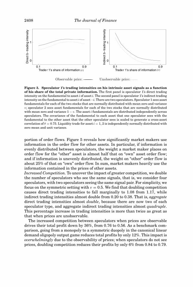
Figure 3 shows how trading intensities vary with a speculator’s share ofprivate information. The figure highlights that trading intensities are farhigher if prices are observable. In part, this reflects that when speculators

9 Lowering correlations raises aggregate profits for any ν, reduces cross-asset trading, andshrinks the consequences of market design.


Observable price: ————————————————————— Unobservable price: Isolated: ------

Figure 1. Total speculator profit as a function of speculator 1’s share of the total privateinformation. There are two speculators. Speculator 1 sees asset fundamentals for each of thetwo stocks that are normally distributed with mean zero and variance ν; speculator 2 sees assetfundamentals for each of the two stocks that are normally distributed with mean zero and variance1 − ν. The asset i fundamentals are distributed independently across speculators. The covarianceof the fundamental to each asset that one speculator sees with the fundamental to the other assetthat the other speculator sees is scaled to generate a cross-asset correlation of θ = 0.75. Liquiditytrade for asset i = 1, 2 is independently normally distributed with zero mean and unit variance.

see prices, they offset the impact of their trades on private signals by subtract-ing their projections on net order flows via γ i. In addition, trading intensitieswith observable prices are higher due to the strategic “order-reduction” effect:Speculators have incentives to increase trading intensities to influence price,which causes other agents to scale down orders, thereby mitigating price im-pacts.

The first panel of Figure 3 reveals that trade on direct information first risesrapidly with a speculator’s information share, before declining as ν is furtherincreased. The second panel shows that indirect trading intensities exhibitan entirely different pattern: When a speculator has little private informa-tion, he uses his asset 1 signal to trade asset 2 extremely aggressively. In fact,when prices are observable and ν = 0.1, speculator 1 uses his noisy signal e1

1of e2

2 to trade asset 2 more aggressively (b21 = 1.56) than speculator 2, who sees

e22(b2

2 = 1.15). This reflects that when ν is small, the expected (squared) size ofspeculator 1’s trade on indirect information, (b2

1)2ν, is far less than (b22)2(1 − ν).

As ν rises, indirect trading intensities fall sharply. Indeed, when prices areunobservable, the speculator with more information trades against his asset 2


Observable price: ————————————————————— Unobservable price:

Figure 2. Speculator 1’s expected profit as a function of his share of the total privateinformation. There are two speculators. Speculator 1 sees asset fundamentals for each of thetwo stocks that are normally distributed with mean zero and variance ν; speculator 2 sees assetfundamentals for each of the two stocks that are normally distributed with mean zero and variance1 − ν. The asset i fundamentals are distributed independently across speculators. The covarianceof the fundamental to each asset that one speculator sees with the fundamental to the other assetthat the other speculator sees is scaled to generate a cross-asset correlation of θ = 0.75. Liquiditytrade for asset i = 1, 2 is independently normally distributed with zero mean and unit variance.

signal when trading asset 1 (see Corollary 1). By doing so, the speculator gainsmore through the influence on the price of asset 2 than he loses through the(small) quadratic loss in market 1 due to his trade against his asset 2 signal.

Figure 4 reveals the “direct” trading weights on the net order flow for theasset being traded first fall slightly (in absolute value) as the speculator’s shareof private information rises and then more than triple in magnitude as ν risesfrom 0.4 to 0.9. That is, the speculator with most of the private informationmore extensively exploits the information in prices in his trading. The oppositepattern arises for “indirect” trading intensities on net order flow, that is, whentraders use information in the order flow for asset 2 to trade asset 1. Indeed,when ν is large, the sign switches. This result reflects that when speculator1 has most of the private information, speculator 2 trades very intensively onhis noisy indirect signals of speculator 1’s information. From 1’s perspective,speculator 2 so overtrades that it changes the sign of the projection.

The trades by speculators on information in prices are predictable by marketmakers—market makers unwind their impact to filter directly the signal-based


0.1 0.9Trader 1's share of information

0

1

Dire

ctb

trad

ing

inte

nsity


0

1

Indi

rect

btr

adin

gin

tens

ity

Observable price: ————————————————————— Unobservable price:

(ν) (ν)

Figure 3. Speculator 1’s trading intensities on his intrinsic asset signals as a functionof his share of the total private information. The first panel is speculator 1’s direct tradingintensity on the fundamental to asset i of asset i. The second panel is speculator 1’s indirect tradingintensity on the fundamental to asset i of asset −i. There are two speculators. Speculator 1 sees assetfundamentals for each of the two stocks that are normally distributed with mean zero and varianceν; speculator 2 sees asset fundamentals for each of the two stocks that are normally distributedwith mean zero and variance 1 − ν. The asset i fundamentals are distributed independently acrossspeculators. The covariance of the fundamental to each asset that one speculator sees with thefundamental to the other asset that the other speculator sees is scaled to generate a cross-assetcorrelation of θ = 0.75. Liquidity trade for asset i = 1, 2 is independently normally distributed withzero mean and unit variance.

portion of order flows. Figure 5 reveals how significantly market makers useinformation in the order flow for other assets. In particular, if information isevenly distributed between speculators, the weight a market maker places onorder flow for the “other” asset is almost half that on “own” asset order flow;and if information is unevenly distributed, the weight on “other” order flow isabout 25% of that on “own” order flow. In sum, market makers heavily use theinformation contained in the prices of other assets.Increased Competition. To uncover the impact of greater competition, we doublethe number of speculators who see the same signals, that is, we consider fourspeculators, with two speculators seeing the same signal pair. For simplicity, wefocus on the symmetric setting with ν = 0.5. We find that doubling competitioncauses direct trading intensities to fall marginally to 1.08 from 1.17, whileindirect trading intensities almost double from 0.20 to 0.38. That is, aggregatedirect trading intensities almost double, because there are now two of eachspeculator type, and aggregate indirect trading intensities almost quadruple.This percentage increase in trading intensities is more than twice as great asthat when prices are unobservable.

The increased competition between speculators when prices are observabledrives their total profit down by 36%, from 0.76 to 0.56. As a benchmark com-parison, going from a monopoly to a symmetric duopoly in the canonical lineardemand oligopoly output game reduces total profits by only 12%. This impact isoverwhelmingly due to the observability of prices; when speculators do not seeprices, doubling competition reduces their profits by only 6% from 0.84 to 0.79.



0.5

0

0.1D

irect

γ w

eigh

t

Indi

rect

γ w

eigh

t


0.5

0

0.1

(ν) (ν)

Figure 4. Speculator 1’s trading intensities on prices as a function of his share of totalprivate information. The first panel is speculator 1’s trading intensity on price pi of asset i.The second panel is speculator 1’s indirect trading intensity on price pi of asset −i. There are twospeculators. Speculator 1 sees asset fundamentals for each of the two stocks that are normallydistributed with mean zero and variance ν; speculator 2 sees asset fundamentals for each of thetwo stocks that are normally distributed with mean zero and variance 1 − ν. The asset i fundamen-tals are distributed independently across speculators. The covariance of the fundamental to eachasset that one speculator sees with the fundamental to the other asset that the other speculatorsees is scaled to generate a cross-asset correlation of θ = 0.75. Liquidity trade for asset i = 1, 2 isindependently normally distributed with zero mean and unit variance.


0

0.5

Dire

ct µ

coe

ffici

ent


0

0.5

Indi

rect

µ c

oeffi

cien

t

(ν) (ν)

Figure 5. The coefficients of the market maker’s effective pricing filter, µ=λΓ, as afunction of the share of total private information that speculator 1 has. The first panel isthe coefficient on net order flow of asset i for the pricing of asset i. The second panel is the coeffi-cient on net order flow of asset i for the pricing of asset −i. There are two speculators. Speculator1 sees asset fundamentals for each of the two stocks that are normally distributed with mean zeroand variance ν; speculator 2 sees asset fundamentals for each of the two stocks that are normallydistributed with mean zero and variance 1 − ν. The asset i fundamentals are distributed indepen-dently across speculators. The covariance of the fundamental to each asset that one speculatorsees with the fundamental to the other asset that the other speculator sees is scaled to generatea cross-asset correlation of θ = 0.75. Liquidity trade for asset i = 1, 2 is independently normallydistributed with zero mean and unit variance.

The differential impacts of increased competition on speculator profit whenprices are and are not observable reflect the differential impacts on tradingintensities.Price Correlations. Figure 6 displays how the cross-asset correlation in pricechanges varies with ν. In contrast to the correlation of information across


Observable price: ————————————————————— Unobservable price: Isolated: ------

Figure 6. The ratio of the correlation in asset prices to the underlying correlation inasset values. There are two speculators. Speculator 1 sees asset fundamentals for each of thetwo stocks that are normally distributed with mean zero and variance ν; speculator 2 sees as-set fundamentals for each of the two stocks that are normally distributed with mean zero andvariance 1 − ν. The asset i fundamentals are distributed independently across speculators. Thecovariance of the fundamental to each asset that one speculator sees with the fundamental to theother asset that the other speculator sees is scaled to generate a cross-asset correlation of θ = 0.75.Liquidity trade for asset i = 1, 2 is independently normally distributed with zero mean and unitvariance.

speculators, which is fixed at 0.75, the cross-asset correlation θ√

ν(1 − ν)/2 risesas ν → 1/2. Consequently, in the figure we normalize price correlations by di-viding by the asset value correlation.

Strikingly, in integrated stock markets, prices are far more correlated thanthe underlying asset values, but in isolated markets, prices are far less corre-lated. This reflects that market makers in integrated markets digest the infor-mation in order flows for all assets when pricing. This cross-asset correlationraises the volatility of prices in integrated markets.10 Cross-asset correlationsare higher yet when speculators see prices, because speculators trade more ag-gressively on their cross-asset information. The price volatility consequencesof the informational environment are substantial. For example, when informa-tion is evenly divided between speculators, the variance of price changes is 19%higher when prices are observed by speculators than when they are not.

10 This indicates that failing to account for market integration on an individual stock basis biasespredicted price variances downward.


0.1 0.9Asset 1 share of liquidity trade

0

2D

irect

b–tr

adin

gin

tens

ity

0.1 0.9Asset 1 share of liquidity trade

0

2

Indi

rect

btr

adin

gin

tens

ity

Figure 7. Direct and indirect trading intensities of asset 1 as a function of market1’s share of the total standard deviation of liquidity trade across assets. There are twospeculators. Speculator 1 sees asset fundamentals for each of the two stocks that are normallydistributed with mean zero and standard deviation 1

2 ; speculator 2 sees asset fundamentals foreach of the two stocks that are normally distributed with mean zero and standard deviation 1

2 .The asset i fundamentals are distributed independently across speculators. The covariance of thefundamental to each asset that one speculator sees with the fundamental to the other asset that theother speculator sees is scaled to generate a cross-asset correlation of θ = 0.75. The total standarddeviation of liquidity trade across the two markets is 2.

B. Division of Liquidity Trade across Assets

We now explore how the division of liquidity trade affects outcomes. Thatis, we address what happens when one asset has more liquidity trade be-hind which speculators can hide their trades. To do so, we consider symmet-rically distributed asset values and symmetrically situated speculators. Wethen vary the share of the standard deviation of liquidity trade between theassets.

We find that total expected speculator profits are remarkably insensitive tothe division of liquidity trade between assets. Maintaining a total standard de-viation of liquidity trade across assets of 2.0, going from a setting in which eachasset has liquidity trade of 1.0 to a very unbalanced distribution of liquiditytrade where asset 1 has a standard deviation of liquidity trade of 1.45, raisesspeculator profits by only 2%. That is, in stark contrast to the impact of the divi-sion of information between speculators, the division of liquidity trade betweenassets has trivial consequences for speculator profits, even when speculatorssee prices.

However, Figure 7 shows that the division of liquidity trade affects how spec-ulators trade on their signals. Increasing asset 1’s share of liquidity trade from0.1 to 0.9 causes speculators to double direct trading intensities on asset 1 sig-nals; when asset 1 has almost all of the liquidity trade, speculators use theirasset 2 signal to trade both assets equally aggressively, and they trade againstasset 1 signals in the illiquid asset 2 market. Still, liquidity trade must be veryasymmetrically divided before speculators trade against their indirect signalsin the less liquid market. In contrast, if speculators do not see prices, theyalways trade against their indirect signals in the less liquid market. When


0.1 0.9Asset 1 share of standard deviation

0

2D

irect

b–tr

adin

gin

tens

ity

0.1 0.9Asset 1 share of standard deviation

0

2

Indi

rect

b–tr

adin

gin

tens

ity

Figure 8. Direct and indirect trading intensities of asset 1 as a function of asset 1’sshare of the total standard deviation of private information across assets. There are twospeculators. The total standard deviation of private information across assets is 2. The speculatorseach see a fundamental to asset 1 that is distributed normally and independently of the otherspeculator’s signal of asset 1, with a mean of zero and a standard deviation that varies between1 and 1.45. The speculators each see a fundamental to asset 2 that is distributed normally andindependently of the other speculator’s signal, with a mean of zero and a standard deviation suchthat the sum across assets is 2. The covariance of the fundamental to each asset that one speculatorsees with the fundamental to the other asset that the other speculator sees is scaled to generatea cross-asset correlation of θ = 0.75. Liquidity trade for asset i = 1, 2 is independently normallydistributed with zero mean and unit variance.

speculators see prices, they are more willing to trade in the same directionas their signals because they can unwind the trade’s projection onto net orderflows, mitigating price impacts.

C. Division of Uncertainty between Assets

We next explore how the division of uncertainty across assets affects out-comes. That is, we address what happens when there is more private informa-tion about asset 1’s value than asset 2’s. To do so, we assume that speculatorsare symmetrically situated, and the distribution of liquidity trade is the sameacross assets. We fix the total standard deviation of liquidity trade to 2.0 andthen progressively increase the standard deviation of asset 1 from 1.0 to 1.45.

We find that total expected speculator profits are as insensitive to the divisionof private information between assets as they are to the division of liquiditytrade. More asymmetric divisions of private information between assets leadto higher profits, but there is only about a 2% difference between profits whenuncertainty is evenly and very unevenly divided.

Figure 8 reveals that speculators trade more aggressively on their signal forthe less volatile asset both directly and indirectly. Also, as with very unevenlydistributed liquidity trade, if information is very unevenly divided betweenassets, speculators trade against their more volatile asset signal of the lessvolatile asset’s value. In sum, the division of information between assets mat-ters in complicated ways for trading strategies, but not aggregate outcomes.


IV. Conclusion

This paper develops a method to solve for strategic speculative outcomes in amulti-asset stock market when speculators see prices and internalize how theirtrades affect the informational content of prices. We thereby build on Admati’s(1985) noisy rational expectations model to allow for strategic behaviour byspeculators. In particular, speculators in our model internalize the fact thatthey are informationally large and that their trades have impacts on prices thatconvey information to other speculators. Because asset values are correlated,a signal about one asset contains information about other assets, and becausethere are multiple speculators, each speculator uses the information in pricesto try to unravel the signals of others. We prove that there is a unique linearequilibrium by developing an iterative best-response mapping and showing thatit is a contraction.

We then offer several testable predictions. We generate predictions about thecovariance structures of prices changes (returns) and order flows across stocksthat are driven solely by strategic behaviour. In particular, we find that thecovariance structure of prices is driven by the covariance structure of assetfundamentals, while the covariance structure of order flows is driven by thecovariance structure of liquidity trade. We also show that in integrated markets,the use of cross-asset information by market makers causes prices to be morecorrelated than the underlying fundamentals, and that this, in turn, raisesthe volatility of prices. Finally, we provide theoretical underpinnings for theHasbrouck and Seppi (2001) finding that commonality in order flows explainstwo-thirds of the commonality in returns, generating this in our model witha moderate cross-asset correlation in asset value fundamentals plus a slightpositive correlation in liquidity trade across assets.

While one must be careful translating predictions from a stylized model tothe real world, the qualitative implications are clear. The transparency of pric-ing and order flows across assets has greatly increased in recent years. Thissuggests that the market has become “closer” to our observable price setting.Accordingly, (a) the volatility of returns and net order flows should have in-creased, and (b) the contemporaneous correlation in returns (e.g., within in-dustries) should have risen, but (c) the contemporaneous correlation in orderflows should not.

Our companion numerical analysis provides insights into the quantitativelyimportant aspects of (a) the informational structure of the market and (b) thedistributions over fundamentals, private information, and liquidity trade. Theobservability of prices sharply lowers speculator profits, especially when morespeculators compete over the same information. This is because prices provideadditional channels through which speculators receive and transmit informa-tion, giving each speculator incentives to raise trading intensities to influencethe trades of other speculators. As a result, the observability of prices enhancesthe sensitivity of total speculator profits to the division of information betweenspeculators. In sharp contrast, the divisions of liquidity trade and uncertaintyacross assets have little effect on aggregate speculative profits. In sum, the


division of private information between speculators matters for aggregate out-comes, but the division of information and liquidity between assets does not.

Appendix

Proof of Proposition 1: Use the law of recursive projections to expand the firstterm in the first-order condition (5),

E[v|si, X + u] = E[v|X + u] + E[v − E[v|X + u]|si − E[si|X + u]]

= p + E[v − E[v|X + u]|si − E[e|X + u]],

where the last equality reflects that E[v|(X + u)] = p. By construction, thevector of net order flows X + u is orthogonal to the vector of forecast errorssi − E[si|X + u], so that

E[E[v|X + u]|si − E[si|X + u]] = 0.

Hence, we can remove the conditioning on X + u from the first-order condition(5), which reduces to

0 = E[(p + E[v|si − E[si|X + u]] − p) − qi ′λ′xi|si]

= E[E[v|si − E[si|X + u]] − qi ′λ′xi|si].

Solving for xi yields

xi = (λ′)−1(qi ′)−1 E[E[v|si − E[si|X + u]]].

Q.E.D.

Proof of Lemma 1: Substitute for γ i and � into the first-order condition (5).Recognizing that we do not need to condition on net order flow, u drops out andthe first-order condition becomes

0 = E

[v − λ�

N∑k=1

bksk − qi ′λ′(

bisi + γ iN∑

k=1

bksk

)∣∣∣∣∣si

].

The goal is to remove qi = (I − ∑k =i Bk)−1 from the first-order condition. To do

this, we use

� = I +∑

i

γ i = I +∑

i

Bi

(I −

∑k

Bk

)−1

=(

I −∑

k

Bk +∑

k

Bk

) (I −

∑k

Bk

)−1

= I

(I −

∑k

Bk

)−1

(A1)


and

I + γ i = I + Bi

(I −

∑k

Bk

)−1

=(

I −∑

k

Bk + Bi

) (I −

∑k

Bk

)−1

=(

I −∑k =i

Bk

) (I −

∑k

Bk

)−1

= (qi)−1�.

(A2)

Hence, if we multiply the first-order condition by I + γ i′ = �′(qi′ )−1, the qi termscancel. Q.E.D.

Proof of Proposition 2: First-order condition for λ: Exploiting the fact thatmarket maker expected profits are a scalar, and hence equal to its trace, wefirst rewrite the market maker’s least squares prediction problem as

minλ

tr

V ′ −

N∑k=1

(bk Ak + γ k

N∑�=1

b� A�

)′λ′

−�′λ′

×(

V −N∑

k=1

(bk Ak + γ k

N∑�=1

b� A�

)λ − �λ

) (�e 00 �u

)},

where we have commuted under the trace. The associated first-order conditionis

0 = tr

V ′ −N∑

k=1

(bk Ak + γ k

N∑�=1

b� A�

)′λ′

−(

N∑k=1

γ k + I

)′λ′

×(

−N∑

k=1

(bk Ak + γ k

N∑�=1

b� A�

)−

(N∑

k=1

γ k + I

)) (�e 00 �u

)}

= tr

{(−

N∑k=1

(bk Ak + γ k

N∑�=1

b� A�

)−

(N∑

k=1

γ k + I

))

×(

�e 00 �u

)

V ′ −N∑

k=1

(bk Ak + γ k

N∑�=1

b� A�

)′λ′

−(

N∑k=1

γ k + I

)′λ′

, (A3)


where we commuted under the trace. We now compute the trace to rewrite (A3)compactly as

(−�bA − �)(

�e 00 �u

) (V ′ − A′b′�′λ′

−�′λ′

)= 0

⇒ �(bA I )(

�e 00 �u

) (A′b′

I

)�′λ′ = �(bA I )

(�e 00 �u

) (V ′

0

). (A4)

The speculator’s optimization problem. We first rewrite the speculator’s objec-tive, commuting under the trace to obtain

maxbi ,Bi

E

tr

V − λ�

N∑k=1

bk Ak − λ�

′ bi Ai + γ i

N∑

k=1

bk Ak

γ i

(

eu

)(e′ u′)

= maxbi ,Bi

tr

V ′ −

N∑k=1

Ak′bk′

�′λ′

�′λ′

(bi Ai + γ i

(N∑

k=1

bk Ak

)γ i

) (�e 00 �u

) .

(A5)

First-order conditions for bi.

0 = tr

V ′ −

N∑k=1

Ak′bk′

�′λ′

−�′λ′

(Ai + γ i Ai 0)

(�e 00 �u

)

−(

Ai′�′λ′

0

)(bi Ai + γ i

N∑k=1

Akbk γ i)(

�e 00 �u

)}

= tr

V ′ −

N∑k=1

Ak′bk′

�′λ′

−�′λ′

(Ai + γ i Ai 0)�e −

(Ai′

�′λ′

0

)

×((

bi Ai + γ iN∑

k=1

Akbk

)�e γ i�u

)}.

The off-diagonals drop out due to the trace operation, leaving

0 = tr

{(V ′ −

N∑k=1

Ak′bk′

�′λ′)

(Ai + γ i Ai)�e − (Ai′�′λ′)

(bi Ai + γ k

N∑k=1

Akbk

)�e

}.

We now manipulate the first-order condition to isolate the {bk} terms. The traceis preserved under transposition: Taking the transpose of the second term and


then commuting under the trace yields

0 = tr

{Ai�e

(V ′ −

N∑k=1

Ak′bk′

�′λ′)

(I + γ i) − �e

(bi Ai + γ i

N∑k=1

Akbk

)′λ�Ai

}

= tr

{Ai�e

(V ′ −

N∑k=1

Ak′bk′

�′λ′)

(I + γ i) − Ai�e

(bi Ai + γ i

N∑k=1

Akbk

)′λ�

}

⇒ Ai�e

N∑k=1

Ak′bk′

�′λ′(I + γ i) + Ai�e

(Ai′

bi′ +N∑

k=1

Ak′bk′

γ i′)

λ�

= Ai�eV ′(I + γ i).

First-order condition for Bi. We first note that

∂γ i

∂ Bi =(

I −∑

k

Bk

)−1

+ Bi

(I −

∑k

Bk

)−2

= (I + γ i)� and ∂�∂ Bi = �2.

Differentiating (18) with respect to Bi and setting it equal to zero yields

0 = tr

V ′ −N∑

k=1

(bk Ak + γ k

N∑�=1

b� A�

)′λ′

−(

N∑k=1

γ k + I

)′λ′

∂γ i

∂ Bi

(N∑

k=1

bk Ak I

) (�e 00 �u

)

− tr

N∑�=1

(b� A�

)′ ∂�′

∂ Bi λ′

∂�′∂ Bi λ

′

(bi Ai + γ i

N∑k=1

bk Ak γ i

) (�e 00 �u

) .

Using the fact that the transpose is the identity under the trace, we rewritethis as:

0 = tr

V ′ −N∑

k=1

(bk Ak + γ k

N∑�=1

b� A�

)′λ′

−(

N∑k=1

γ k + I

)′λ′

∂γ i

∂ Bi

(N∑

k=1

bk Ak I

) (�e 00 �u

)

− tr

(�e 00 �u

)

(bi Ai + γ i

N∑k=1

bk Ak

)′

γ i′

λ ∂�

∂ Bi

(N∑

�=1

(b� A�

)I

) .


Commuting under the trace, we have

0 = tr

∂γ i

∂ Bi

(N∑

k=1

bk Ak I

) (�e 00 �u

)

V ′ −N∑

k=1

(bk Ak + γ k

N∑�=1

b� A�

)′λ′

−(

N∑k=1

γ k + I

)′λ′

− tr

(N∑

�=1

b� A� I

) (�e 00 �u

)

(bi Ai + γ i

N∑k=1

bk Ak

)′

γ i′

λ ∂�

∂ Bi

= ∂γ i

∂ Bi

(N∑

k=1

bk Ak I

) (�e 00 �u

)

V ′ −N∑

k=1

(bk Ak + γ k

N∑�=1

b� A�

)′λ′

−(

N∑k=1

γ k + I

)′λ′

−(

N∑�=1

b� A� I

) (�e 00 �u

)

(bi Ai + γ i

N∑k=1

bk Ak

)′

γ i′

λ ∂�

∂ Bi .

We rewrite this expression more compactly as

0 = ∂γ i

∂ Bi (bA I )(�e 00 �u

)(V ′−A′b′�′λ′

−�′λ′

)

− (bA I )(

�e 00 �u

) (Ai′

bi′ + A′b′γ i′

γ i′

)λ ∂�

∂ Bi

= (I + γ i)�(bA I )(

�e 00 �u

) (V ′ − A′b′�′λ′

−�′λ′

)

− (bA I )(

�e 00 �u

) (Ai′


γ i′

)λ�2.

Inspection of the first term reveals that it is (I + γ i) times the market maker’sfirst-order condition (A4), and hence equal to zero. Thus, the first order condi-tion for Bi simplifies to

(bA I )(

�e 00 �u

) (Ai′


γ i′

)λ�2 = 0

⇒ (bA I )(

�e 00 �u

) (A′b′

I

)γ i′

λ�2 = −(bA I )(

�e 00 �u

) (Ai′

bi′

0

)λ�2.

Carrying out the matrix multiplications yields the solution in (11):

γ i ′ = −(bA�e A′b′ + �u)−1bA�e Ai ′V ′.


Proof of Proposition 3: Defining p =(

0 θ

θ 0

), routine algebra reveals that

∑j =i

Ai�e Aj ′ = p, and Ai�eV ′ = I + p.

Because each bi is identical, symmetric, and countersymmetric in the sensethat the diagonal elements are identical, we can focus on a generic row of thisrecursion, which is a matrix equation:

(I + p)bi′ = pbi′µ(µ′(I + γ i) + (I + γ i′

)µ)−1 + (I + p)(I + γ i)(µ′(I + γ i)

+ (I + γ i′)µ)−1.

(A6)

Before proving the contraction mapping property we need two lemmas.

LEMMA 1: Given symmetry across assets and agents, ‖γ i‖ < 1N , where N is the

number of agents.

Proof :

γ i′ = −(

(bA I )(

�e 00 �u

) (A′b′

I

))−1

(bA I )(

�e 00 �u

) (Ai′

bi′

0

)

= −(

(bA I )(

�e 00 �u

) (A′b′

I

))−1

(bA I )(

�e 00 �u

)1N

(A′b′

0

)

= − 1N

(I − (J ′ J )−1�u).

J′J has positive eigenvalues because it is positive definite, and since it is thesum of two positive definite terms the eigenvalues of �u must be positive butsmaller than the eigenvalues of J′J. Hence, (J′J)−1�u has fractional eigenval-ues, and (I − (J′J)−1�u) must also have fractional eigenvalues (Dhrymes (1978,p. 74.)). Q.E.D.

LEMMA 2: Let Q and R be symmetric 2 × 2 matrices that are also countersymmet-ric, that is, they have identical elements on the diagonals as well. Then QR = RQ.

Proof : Direct computation.

We now bound the nonlinear terms.

LEMMA 3: ‖µ(µ′(I + γ i) + (I + γ i′)µ)−1‖ < 1.

Proof : Using Lemma 2,

µ(µ′(I + γ i) + (I + γ i′)µ)−1 = µ(2(I + γ i)µ)−1 = 1

2(I + γ i)−1.


Because an upper bound on γ i is − 1N I , it follows that∥∥∥∥1

2(I + γ i)−1

∥∥∥∥ <12

∥∥∥∥ NN − 1

∥∥∥∥ < 1. Q.E.D.

We now establish the contraction property of the mapping. Using symmetryacross agents

bA�e A′b′ = bi (I · · · I ) A�e A′

I...I

bi′ = bi N (I + p)bi′

.

Next note that using Lemma 2,

(I + γ i) (µ′(I + γ i) + (I + γ i′)µ)−1 = 1

2µ−1 = 1

2(bA�eV ′)−1(bA�e A′b′ + �u),

where the last equality follows from the definition of µ. Substituting forbA�eA′V ′ and bA�eA′b′ into µ−1 yields

12

µ−1 = 12

(Nbi(I + p))−1(Nbi(I + p)bi′ + �u).

Now substitute for 12µ−1 into the first-order condition for agent i, equation (A6),

to obtain

(I + p)bi′ = pbi′ 12

(I + γ i)−1 + 12

(I + p)(Nbi(I + p))−1(Nbi(I + p)bi′ + �u)

⇒ bi′ = (I + p)−1 pbi′ 12

(I + γ i)−1 + 12

(Nbi(I + p))−1(Nbi(I + p)bi′ + �u).

Multiplying both sides by Nbi(I + p) yields

Nbi(I + p)bi′ = Nbi(I + p)(I + p)−1 pbi′ 12

(I + γ i)−1 + 12

(Nbi(I + p)bi′ + �u).

Next subtract12

Nbi(I + p)bi′from both sides to obtain

12

Nbi(I + p)bi′ = Nbi(I + p)(I + p)−1 pbi′ 12

(I + γ i)−1 + 12

�u.

Since p is diagonal and bi′is symmetric and countersymmetric, then again by

Lemma 2 we can commute (I + p)−1 pbi′to bi′

(I + p)−1 p and divide byN2

to ob-

tain

bi(I + p)bi′ = bi(I + p)bi′(I + p)−1 p(I + γ i)−1 + 1

N�u. (A7)


Defining the 2 × 2 matrix Q ≡ bi(I + p)bi′, we can write equation (A7) as

Q = Q(I + p)−1 p(I + γ i)−1 + 1N

�u.

From Lemma 1

‖(I + γ i)−1‖ < 2.

It is straightforward to establish that the maximum singular value of (I + p)−1pis θ

1−θ. For θ < 1

3 , we then have θ1−θ

< 12 , so that

‖(I + p)−1 p(I + γ i)−1‖ < 1,

implying that the mapping of Q is a contraction. We recover the fixed point ofbi by finding the Cholesky factor of the fixed point of Q and multiplying thatfactor by the inverse of the Cholesky factor of I + p. The Cholesky factor ofI + p is (

1 θ

0 (1 − θ2)12

).

Proof of Proposition 4: Matrices that are both symmetric and countersymmet-ric commute with each other. Exploiting that γ i is symmetric and countersym-metric and identical across agents we multiply the first-order condition for bi,equation (10), by bi and add across i to obtain

bA�e A′b′�′λ′(I + γ i) + 2bi Ai�e Ai′bi′

λ� + bA�ebA′b′γ i′λ�

= bA�eV ′(I + γ i).(A8)

Using the definition of � in (9), we next substitute � − �u in the first term torewrite (A8) as

(� − �u)�′λ′(I + γ i) + 2bi Ai�e Ai′bi′

λ� + bA�e A′b′γ i′λ� = bA�eV ′(I + γ i)

= ��′λ′(I + γ i),

where the last equality follows from the first-order condition for λ, equation(12). Subtracting (� − �u)�′λ′(I + γ i) from both sides yields

2bi Ai�e Ai′bi′

λ� + bA�e A′b′γ i′λ� = �u�′λ′(I + γ i) = �u(I + γ i)�λ,

where the final equality follows from the symmetric-countersymmetric struc-ture of �′λ′ and I + γ i, which allows us first to transpose and then commute.Dividing by λ� then yields

2bi Ai�e Ai′bi′ + bA�e A′b′γ i′ = �u(I + γ i). (A9)


We now use the first-order condition for γ , equation (11), to simplify (A9). Mul-tiplying both sides of (11) by � = bA�eA′b′ + �u and rearranging yields

bA�e A′b′γ i′ = −(�uγ i′ + bA�e Ai′bi′). (A10)

We substitute (A10) for bA�e A′b′γ i′in (A9) and rearrange to obtain

2bi Ai�e Ai′bi′ − bA�e Ai′bi′ = �u(I + 2γ i) = �u�.

Subtracting the common bi Ai�e Ai′bi′

on the left-hand side gives us

bi Ai�e Ai′bi′ − bj =i A j =i�e Ai′bi′ = �u� = �−1�2

u,

where the final equality follows from substituting for � using the first- ordercondition for γ i, equation (11). Multiplying both sides by �−1 then yields

�(bi Ai�e Ai′bi′ − bj =i A j =i�e Ai′bi′) = �2

u. (A11)

We now substitute the structure from the setting of Proposition 2,

Ai�e Ai′ = I and Aj =i�e Ai′ =(

0 θ

θ 0

)≡ p,

to simplify the inner term on the left-hand side of equation (A11),

bi Ai�e Ai′bi′ − bj =i A j =i�e Ai′bi′ = bi(I − p)bi′

= 2bi(I + p)bi′ 12

(I + p)−1(I − p)

= (� − �u)12

(I + p)−1(I − p).

(A12)

The first equality follows because with two agents, bi = bj =i. The second followsfrom commuting I − p with bi′ using symmetry-countersymmetry. The thirduses 2bi(I + p)bi′ = bA�e A′b′ = � − �u. Now substitute for the inner term onthe left-hand side of (A11) using (A12) to obtain

�(� − �u)12

(I + p)−1(I − p) = �2u.

Multiplying both sides by (�−1)2 yields

(I − �−1�u)12

(I + p)−1(I − p) = (�−1�u)2

or

(I − �−1�u)C = (�−1�u)2, (A13)

where

C ≡ 12

(I + p)−1(I − p) = 12(1 − θ2)

(I − p)2

= 12(1 − θ2)

(1 + θ2 −2θ

−2θ 1 + θ2

).

(A14)


Equation (A13) is a quadratic in �−1�u (or equivalently �), and its solutiontakes the general form

��−1u = f (C).

Substituting for � = bA�eA′b′ + �u and rearranging yields

bA�e A′b′ = f (C)�u − �u = ( f (C) − I )�u,

which establishes the result.

Proof of Proposition 5: Using Proposition 4, we have

� = bA�e A′b′ + �u ∼ �1/2u ((A�e A′)−1/2 A�e A′(A�e A′)−1/2 + I )�1/2

u .

Prices are λ(X + u) = λ�(bAe + u), so that the variance–covariance matrix ofprices is

λ�(bA�e A′b′ + �u)�′λ′ = λ��′λ′

= V �e A′b′�−1��−1bA�eV ′

= V �e A′b′�−1bA�eV ′

= (V �e A′b′�−1/2

u)(

�1/2u �−1�

1/2u

)(�

−1/2u bA�eV ′),

where the first equality follows from substituting for λ� from the first-ordercondition (12), and the final equality follows from multiplying and dividing by�

1/2u . The middle term can be written as

(�−1/2

u ��−1/2u

)−1 = (�−1/2u (bA�e A′b′ + �u)�−1/2

u

)−1.

From Proposition 4, b ∼ (A�eA′)−1/2�1/2u , so the �

1/2u terms cancel, leaving only

the effect of �e. Q.E.D.

Proof of Proposition 6: Substitute for λ� using (12) to write the price changecovariance matrix as

V �e A′b′�−1��−1bA�eV ′ = V �e A′b′�−1bA�eV ′. (A15)

We have

V �e A′b′ = 2(

1 θ

θ 1

)bi = 2(I + p)bi, V �eV = 2(I + p),

and bA�e A′b′ = 2bi(I + p)bi ′.

Exploiting the symmetric-countersymmetric structure, we commute and write(A15) as

(V �eV ′)(bA�e A′b′)�−1, (A16)


where V�eV ′ is the value covariance matrix. Now substitute

bA�e A′b′ = � − �u = ( f (C) − I )�u and � = f (C)�u (A17)

from the proof of Proposition 4 into (A16) to obtain

(V �eV ′)( f (C) − I )�u( f (C)�u)−1 = (V �eV ′)( f (C) − I ) f (C)−1. (A18)

To calculate the correlation, we divide by the square root of the product of thediagonal terms: In this symmetric environment, to prove that the correlationin price changes exceeds that in values, we must prove that the ratio of anoff-diagonal element to a diagonal element exceeds θ . To do so, we use thestructure of the solution f(C) for �−1�u = � from equation (A13). Writing (A13)as

C(I − �) = �2, (A19)

we complete the square,

�2 + C� + 14

C2 = C + 14

C2,

and take the square root to solve for

� = −12

C + C1/2(

I + 14

C)1/2

. (A20)

We next use

C(I − �) = �2 ⇒ −(� − I ) = C−1�2

and substitute into (A18) to obtain

(V �eV ′)( f (C) − I ) f (C)−1 = 2(I + p)(� − I )�−1 = −2(I + p)C−1�

= 2(I + p)C−1

(−1

2C + C1/2

(I + 1

4C

)1/2)

= (I + p)(−I + C−1/2(4I + C)1/2).

(A21)

We now use the definition of C in (A14) to calculate the components of(A21):

C−1 = 21 − θ2

(1 + θ2 2θ

2θ 1 + θ2

)and 4I + C = 1

2(1 − θ2)

(9 − 7θ2 −2θ

−2θ 9 − 7θ2

)

⇒ C−1/2 =( 2

1 − θ2

)1/2(

1 θ

θ 1

)and (4I + C)1/2=

( 12(1 − θ2)

)1/2

−a

θ

aθ

a−a

,

where a2 = 9 − 7θ2 + [(9 − 7θ2)2 − 4θ2]1/2

2, with a > 0 the relevant solution to


a4 + θ2 − (9 − 7θ2)a2 = 0. Substituting into (A21) yields

(V �eV ′)( f (C) − I ) f (C)−1

=(

1 θ

θ 1

) −I +

(2

1 − θ2

)1/2 (1 θ

θ 1

) (1

2(1 − θ2)

)1/2

−a

θ

aθ

a−a

=(

1 θ

θ 1

) −I +

(1

1 − θ2

) (1 θ

θ 1

) a − θ

a− θ

aa

∼(

1 θ

θ 1

)

(−(1 − θ2) 00 −(1 − θ2)

)+

(1 θ

θ 1

) a − θ

a− θ

aa

∼(

1 θ

θ 1

)

−(1 − θ2) + a − θ2

aaθ − θ

a

aθ − θ

a−(1 − θ2) + a − θ2

a

∼

−(1 − θ2) + a − θ2

a+ aθ2 − θ2

aθ

(−(1 − θ2) + 2a − θ2

a− 1

a

)

θ

(−(1 − θ2) + 2a − θ2

a− 1

a

)−(1 − θ2) + a − θ2

a+ aθ2 − θ2

a

.

Hence, the off-diagonal/diagonal ratio exceeds θ if

−(1 − θ2) + 2a − θ2

a− 1

a> −(1 − θ2) + a − θ2

a+ aθ2 − θ2

a⇔ a − 1

a> θ2

(a − 1

a

),

which holds as long as assets are not perfectly correlated. Substituting θ → 0into the off-diagonal/diagonal ratio yields 5

3θ , which our numerical analysisconfirms. Q.E.D.

Proof of Proposition 7: The variance–covariance matrix of net order flows is�(bA�eA′b′ + �u)�′. We first simplify the solution for �. From equation (11), wehave

� = I +∑

i

γ i = I −((

bA I) (

�e 00 �u

) (A′b′

I

))−1

(bA I )

×(

�e 00 �u

) (A′b′

0

).


Adding and subtracting ((bA I )(�e 00 �u

)(A′b′

I ))−1�u, we write � as

� = I −(

(bAI )(

�e 00 �u

) (A′b′

I

))−1

(bAI )(

�e 00 �u

) (A′b′

I

)

+(

(bA I )(

�e 00 �u

) (A′b′

I

))−1

�u

= I − I +(

(bAI )(

�e 00 �u

) (A′b′

I

))−1

�u

=(

(bAI )(

�e 00 �u

) (A′b′

I

))−1

�u.

We use this solution for � to simplify the variance–covariance matrix of netorder flows,

�(bA�e A′b′ + �u)�′ = �(bA�e A′b′ + �u)�−1u �u�′ = ��−1�u�′ = �u�′.

In the fully symmetric two-speculator setting, � does not depend on �e (seeProposition 6).

Proof of Proposition 8 (Unobservable prices): The variance–covariance matrixof net order flows is (bA�eA′b′ + �u): With uncorrelated liquidity trade �u isdiagonal, so that the off-diagonal terms equal their values in bA�eA′b′. FromCorollary 1, with symmetry, speculators only trade on their direct signals andthey trade with the same intensity on each direct signal. Hence,

bA�e A′b′ =(

b11 0 b11 00 b11 0 b11

)

1 0 0 00 0 1 00 1 0 00 0 0 1

12

0 0θ

2

012

θ

20

0θ

212

0

θ

20 0

12

×

1 0 0 00 0 1 00 1 0 00 0 0 1

b11 00 b11

b11 00 b11

=(

b11 0 b11 00 b11 0 b11

)

12

0 0θ

2

012

θ

20

0θ

212

0

θ

20 0

12

b11 00 b11

b11 00 b11

= (b11)2(

1 θ

θ 1

).


REFERENCESAdmati, Anat, 1985, A noisy rational expectations equilibrium for multi-asset securities markets,

Econometrica 53, 629–658.Admati, Anat, and Paul Pfleiderer, 1988, A theory of intraday patterns: Volume and price variabil-

ity, Review of Financial Studies 1, 3–40.Bernhardt, Dan, and Eric Hughson, 1997, Splitting orders, Review of Financial Studies 10, 69–101.Bernhardt, Dan, and Reza Mahani, 2007, Asymmetric information and stock return cross-

autocorrelations, Economics Letters 96, 14–22.Bernhardt, Dan, Bart Taub, and Peter Seiler, 2007, Speculative dynamics Working paper, Univer-

sity of Illinois.Biais, Bruno, Larry Glosten, and Chester Spatt, 2005, Market microstructure: A survey of micro-

foundations, empirical results and policy implications, Journal of Financial Markets 8, 217–264.

Biais, Bruno, David Martimort, and Jean-Charles Rochet, 2002, Competing mechanisms in a com-mon value environment, Econometrica 68, 799–837.

Caballe, Jordi, and Murugappa Krishnan, 1994, Imperfect competition in a multi-security marketwith risk neutrality, Econometrica 62, 695–704.

Chan, Kalok, 1993, Imperfect information and cross-autocorrelation among stock prices, Journalof Finance 48, 1211–1230.

Chordia, Tarun, and Bhaskaran Swaminathan, 2004, Incomplete information, trading costs andcross-autocorrelations in stock returns, Economic Notes 33, 145–181.

Chowhdry, Bhagwan, and Vikram Nanda, 1991, Multimarket trading and market liquidity, Reviewof Financial Studies 4, 483–511.

Dennert, Jurgen, 1993, Price competition between market makers, Review of Economic Studies,60, 735–751.

Dhrymes, Phoebus, 1978, Mathematics for Econometrics (Springer, NY).Hasbrouck, Joel, and Duane Seppi, 2001, Common factors in prices, order flows, and liquidity,

Journal of Financial Economics 59, 383–411.Hellwig, Martin, 1980, On the aggregation of information in competitive markets, Journal of Eco-

nomic Theory 22, 477–498.Kyle, Albert, 1985, Continuous auctions and insider trading, Econometrica 53, 1315–1335.Kyle, Albert, 1989, Informed speculation and monopolistic competition, Review of Economic Studies

56, 317–355.Malinova, Katya, and Lones Smith, 2003, Dynamic rational expectations equilibrium with private

information: How not to forecast the forecasts of others, working paper, University of Michigan.Pearlman, Joseph, and Thomas Sargent, 2005, Knowing the forecasts of others, Review of Economic

Dynamics 8, 480–497.Townsend, Robert, 1985, Forecasting the forecasts of others, Journal of Political Economy 91, 546–

588.

cross-asset speculation in stock markets

Documents