Cross-Country Determinants of Declines in Infant Mortality:

A Growth Regression Approach*

Stephen D. Younger Cornell University

Food and Nutrition Policy Program

December, 2001 *I am grateful to USAID for financial support through cooperative agreement #AOT-0546-A-00-378-00. I also thank Bill Easterly for suggestions on data and on a “consensus” growth regression, and Rumki Saha for excellent research assistance.

Introduction The past decade has seen a profusion of research that estimates growth regressions.1 Using cross-sections or short cross-country panels, these models regress the growth in real per capita income on real per capita income in a base year and other possible determinants of economic growth. While some of the questions that this research addresses are of theoretical interest, most notably the question of conditional convergence of real incomes across countries, most of the papers are quite practical, attempting to inform policy by identifying variables that explain growth rates. It is easy to be skeptical of these regressions. Specifications are often ad hoc. Many regressors would seem to be endogenous, but are not instrumented, or are instrumented poorly. And early on, there was clear indication that results are not robust. Levine and Renelt (1992) showed that almost all of the regressors that authors have proposed as important determinants of economic growth do not survive an extreme bounds analysis (Leamer, 1983).2 These problems are compounded by the abundance of potential explanatory variables that authors have proposed – Durlauf and Quah (1999) found more than 90 in a recent review of the literature – and the relative scarcity of data, there being only about 120 countries with data available for the basic set of regressors. In such an environment, statistics alone cannot determine the appropriate model of growth determinants.

Despite these limitations, many of the growth regression papers have figured prominently in the debate about economic policy and economic growth. Some economists, and probably more policy makers, have been persuaded of the value of open trade (Dollar and Kraay, 2001), low budget deficits (Easterly and Levine, 1997), financial deepening (Levine and Zervos, 1998), and an educated workforce (Barro and Lee, 1994).

In this paper, I pursue the growth regression model, warts and all, but with a change of variable. Rather than explaining increases in GDP per capita, I attempt to explain decreases in the infant mortality rate. There are four reasons for doing this, two conceptual and two econometric. The first conceptual justification follows Sen (1979, 1985, 1987). The traditional economics literature gauges poverty in terms of deprivation of means, income, which at a national level leads naturally to an analysis of GDP and its determinants. Sen argues instead for viewing poverty as a deprivation of ends (capabilities and functionings, in his terms) that are intrinsically important. Certainly, survival is a basic capability, so that infant mortality is an interesting indicator of well being, worthy of study in its own right. Just as understanding the determinants of infant mortality at a micro level is a valuable exercise (Stifel, Sahn, and Younger 2000), so too is understanding the determinants of infant mortality rates at a national level. While this in no way supposes that infant mortality (or any other outcome) should replace income as the

1 There are far too many empirical growth papers to list them here or anywhere in this paper, but a good place to start is Durlauf and Quah, 1999. The references that I include are illustrative papers; many more are available. 2 Leamer’s extreme bounds analysis runs many regressions with different specifications, including different regressors, keeping only the regressors of interest in all specifications. It then checks to see that the coefficient on these regressors are stable in the many different specifications, and if they remain statistically significant.

2

measure of welfare, it certainly seems sensible to include it as one such measure. This paper begins such a study.

The second conceptual reason for studying infant mortality is that its distributional characteristics are almost certainly more sensitive to the welfare of the poor (Pradhan, Sahn, and Younger, 2001). As welfare broadly conceived rises, both income and mortality probabilities fall, but the relationship between the two is surely not linear. Incomes can continue to rise indefinitely, while mortality probabilities have an obvious lower bound. An important implication of this fact is that improvements in welfare, for individuals or nations, are more likely to be associated with improvements in mortality if welfare is low, whereas there is no obvious correlation between welfare improvements and the initial level of income. For at least some policy discussions, particularly those that are concerned with how a nation’s progress reduces poverty, the greater emphasis on the poorest implied by a focus on mortality is desirable.

The first econometric justification for this paper’s approach follows an argument in Jones

(1995). In a standard growth regression, the dependent variable (growth in real per capita GDP) is probably stationary, that is, it stays around a given rate, tending back to that rate when it is either higher or lower. On the other hand, the log of real per capita GDP, one of the independent variables in a growth regression, is not stationary; it increases regularly and has no tendency to decline once it has increased. Even if the regression produces a partial correlation between growth and the level of GDP, such a correlation is almost surely spurious, since one variable that stays stationary around a given value cannot move consistently with another that trends upward (Granger and Newbold, 1974). The only possible exception to this observation is if the non-stationary regressor is fortuitously cointegrated with the other regressors, so that the entire right-hand side of the regression is stationary when the effects are netted out. Both Jones (1995) and Easterly (2000) suggest that this is not the case, so then the regression is likely to be spurious. Infant mortality rates, however, are stationary. Logically, they must hit a lower bound of zero at some point. Empirically, I show that the autocorrelation of IMRs is fairly low, and that formal tests reject the null of a unit root in the IMR or its log.

Finally, an important problem with growth regressions is that there are relatively few data

to run them on. Barro’s original regression used average growth rates over 25 years for one cross-section of countries. The argument for this is that we want to estimate long-run structural determinants of growth, not short-run autocorrelations driven by the business cycle. In practice, however, many subsequent papers have used panels of growth rates over decades or even five-year periods rather than a simple cross-section in order to generate more observations. Given the high autocorrelation of real GDP, this is a risky practice. Conceptually, the infant mortality rate seems less likely to be influenced by the business cycle or other high-frequency events. As we will see, autocorrelations for IMRs are much lower than those for GDP, so that panels drawn for periods perhaps as short as five years are more defensible.

The layout of the paper is as follows. The following section lays out the specification of

the standard growth regression model, and explains how I will mimic it for IMRs in this paper. This section also compares this specification to regressions of IMRs on their determinants found in the literature. I then explore the time series properties of IMRs, followed by the results for the main model of IMRs.

3

Specification of a “Growth Regression” Model of Declines in Infant Mortality The aim of this paper is to estimate a cross-country model for declines in infant mortality using a growth regression specification. The basis for that specification is very simple, though it is often overlooked.3 The growth rate is taken to be a linear function of the gap between current GDP per capita and a steady state level of GDP:

tttt

t yydtdyg εββ +−+== )( *

10 (1)

where yt is the log of current GDP per capita; y* is its steady state growth path; gt is the current growth rate; β1 is the rate at which yt converges to y*; and β0 is the exogenous growth rate of y* (the rate of technical progress). Few empirical growth papers start with this simple equation, so they tend to lose site of an important econometric point: yt and y* are almost certainly non-stationary processes, while gt is probably stationary.4 For equation (1) to make sense, then, yt and y* should be cointegrated, a point first noted by Jones (1995). If they are not, then there is a risk of spurious regression. The dependent variable is stationary while the right-hand side of the regression will wander off indefinitely, making it implausible that any estimated correlation captures a true structural relationship. Of course, y* is unobservable, so we must write it as a function of some observable variables

ttt uXy += γ* (2)

which allows practitioners to include policy variables as determinants of economic growth:

ttttttttt

t uXyuXydtdyg εβγβββεγββ ++−+=++−+== 111010 )(

ttttttt ebXyuXy +−+=++−+= 11010 )( ββεγββ (3) We can argue, for example, that countries with policies that encourage greater financial depth are on higher steady-state growth paths than those with shallow financial markets. For a given yt, this higher value of y* will induce more rapid growth because of the larger gap between the two. This phenomenon is only temporary since, once the gap is closed, the country’s growth will converge to the normal rate. But most empirical evidence suggests that this convergence is very slow, so that better policy (or any other advantageous Xt) will improve growth for a long time (Barro and Sala-i-Martin, 1999). In this case, yt and Xt must now be cointegrated, but there is little support for that in data (Jones, 1995; Easterly, 2000). Of course, growth regressions generally use cross-section data rather than a time series for an individual country. But the only way to justify such regressions is to assume that each country observation is a draw from a

3 Barro and Sala-i-Martin (1999, ch.12) give a clear presentation. 4 The next section supports these claims empirically.

4

unique stochastic growth process, so that the time series concepts should apply to the cross-section data. Unlike GDP, infant mortality rates are likely to follow a stationary process. At the extreme, they have to, because the rate cannot go below zero.5 In this case, yt, y*, and gt are all stationary variables, and there is no risk of spurious regression in the sense of Granger and Newbold. The intuition for the model is exactly the same. Policy variables determine the steady-state IMR and its rate of change is a function of the distance between the current and steady-state IMRs. There are, of course, other papers that use cross-country data to estimate the determinants of infant mortality rates. Until recently, almost all used a specification like:

ttt XIMR εγ += (4) that is, the IMR itself as a function of policy (and other) variables. This specification, however, does not capture the dynamics inherent in a growth regression. In addition, there is an econometric risk that country- or time-specific fixed effects can easily lead to a spurious correlation (Easterly, 2000). To account for this problem, Pritchett and Summers (1996) include fixed effects for country and time in a panel regression, though there interest is confined primarily to the relationship between the IMR and income per capita rather than policy variables. Similarly, Easterly (1999) uses either county fixed effects or first differences of equation (4), but using only per capita income as a regressor. In terms of specification, then, the innovation of this paper is to capture the convergence of IMRs in a growth regression framework, and to include policy variables among the regressors that help to explain infant mortality rates.

Time Series Characteristics of Infant Mortality Rates Figure 1 shows the infant mortality rates drawn from three years of the Global Development Network’s growth database (Easterly and Sewadeh, 2001), ordered from highest to lowest. The data shift down over time, which reflects general technological progress in the prevention of infant mortality, and for all but perhaps the 1962 data, they are clearly convex, suggesting that the IMR is indeed stationary. Unfortunately, these can be no more than illustrative, because there is no justification for ordering a cross-section of countries in this way. Further, as Bhargava, et.al. (2001) point out, the publicly available, country-specific IMR series include projections and/or interpolations, so that a time series analysis using them would be just as likely to pick up the rules used for projecting the data as their true time series characteristics. Fortunately, there is an alternative data source that provides reasonable and comparable time series for infant mortality rates. The Demographic and Health Surveys (Macro International) include careful birth and death information for all the children born to a random sample of women of childbearing age (15-49 years old). 151 DHS surveys have been or are

5 Again, the next section supports this claim empirically.

5

being carried out in 68 countries, using virtually identical questionnaires. Using this information, it is possible to estimate a time series of IMRs going back t years for children born to women age 15 to (49-t). This sample continues to be random because being of an age between 15 and 49-t did not figure in the selection, but it is for a smaller population of women. Since infant mortality usually declines with mother’s age, the IMR estimates here may be a little high. While there might be some concern about the accuracy of recall over long periods of time, a child’s birth or death is an unlikely thing to forget. In practice, IMRs calculated with the DHS data correspond well to information in other sources, with no clear bias up or down for lags up to 10 years (Sahn, Stifel, and Younger, 2000). In what follows, I use the same 10-year lag length, so that I am calculating IMRs for children born to women ages 15-39. The data form an unbalanced panel of 82 DHS surveys.6 Im, Pesaran, and Shin (1997) derive the sampling distribution for a “t-bar” statistic to test the null hypothesis of a unit root in heterogeneous panels of time series data.7 This statistic is applicable to an average of the t-statistics from individual Dickey-Fuller regressions for each country:

ttttt dIMRdIMRIMRdIMR εββα +++= −−− ...22111 (5) where IMR is the infant mortality rate, dIMR is its change from period t-1 to t, and α is one minus the autocorrelation coefficient. If α is zero, then the series has an autocorrelation of one, or a unit root, and is thus nonstationary. Thus, the Dickey-Fuller test tests the null hypothesis that α equals zero. In addition to the lagged level of the IMR, it is important to include enough lagged dependent variables (dIMRs) to ensure that the regression’s error, ε, has no remaining serial correlation. The Im, Pesaran, and Shin test elaborates on the Dickey-Fuller test by calculating the t-value for α in a regression for each sample, and averaging them. This statistic does not have a standard t distribution, but the authors calculate its distribution, allowing tests of the null hypothesis that the series do not contain unit roots.

Unfortunately, the fact that there are only eight or nine observations per country in my sample gives this test very little power, and does not reject the null hypothesis of a unit root for the IMR or its log, even though the average estimated autocorrelation is only 0.30 and 0.33, respectively. However, if we accept the assumption that all countries’ data are drawn from the same process, then we can pool the data to examine the serie’s autocorrelations and also perform standard Dickey-Fuller tests. This may seem a strong assumption, but it is one that we will have to make to justify cross-country growth regressions, so there is no additional harm in making it here. This amounts to running one augmented Dickey-Fuller regression only, using the standard test for a unit root, and allowing each sub-sample to have its own intercept:

tttjjtt dIMRdIMRDIMRdIMR εββδα +++= −−− ...22111 (6)

6 The panel is unbalanced because not all DHS surveys are carried out at the same time in a calendar year. This means that in mapping the birth and death data to calendar years, some years have very few observations. We dropped years in which the number of observations was less than 200. 7 In time series analysis, series with a unit root are not stationary, while those whose roots are all less than one are stationary.

6

where the Dj’s are sample-specific dummies. Using up to six lags, the augmented Dickey-Fuller tests consistently reject the null of a unit root with high t-statistics, with or without a linear or quadratic trend in the regression.

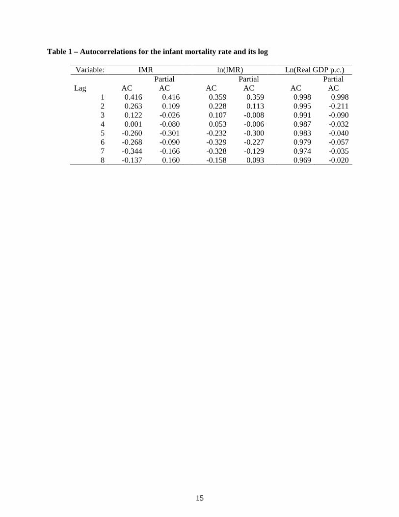
Table 1 shows the autocorrelations of IMRs and their log. An AR(1) process seems adequate to describe both series, with the autocorrelation coefficient being small, at least by business cycle standards. With an autocorrelation of 0.42, for example, the correlation between an IMR and its three-year lag is only 0.03, suggesting that whatever “business cycle” effects there are in these data are of relatively high frequency, so that aggregations of five- or even three-year periods will capture structural rather than cyclical effects of regressors on the IMR.

For comparison, I also performed the Im, Pesaran, and Shin test on the log of real per capita GDP taken from the GDN data. This test also accepts the null of a unit root, whether or not a trend is included in the Dickey-Fuller regression. In this case, there are many more observations per country, 34 on average, and the estimated autocorrelation is about 0.93 (0.81 for the models with trends), so there is less reason to worry about the power of the test. Nevertheless, analogous to the IMR tests, I pooled the country time series to test for a unit root with the traditional Dickey-Fuller test, assuming that each countries’ data are draws from a common process. These tests also reject the null of a unit root, whether or not a trend is included, but with estimates of the autocorrelation coefficient that are between 0.95 and 0.97, sufficiently close to one to call into question the growth regression specification for this variable. Certainly the sample autocorrelations shown in Table 1 lead to the same conclusion.

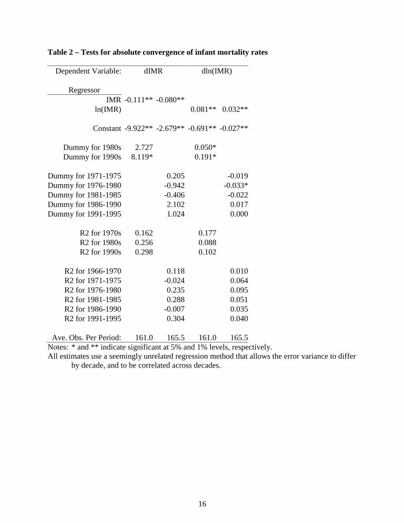
Cross-Country Infant Mortality Regressions Absolute Convergence The growth regression literature quickly dismissed the hypothesis that countries’ GDP per capita converges absolutely (Kormendi and Meguire, 1985). There is no evidence that poor countries grow faster than rich ones without controlling for other factors, among them endowments and policies. The same is not true for infant mortality rates. Table 2 reports regressions that test for absolute convergence of infant mortality rates and their log. These data now come from the Global Development Network growth database rather than the DHS, so they include a broad range of developed and developing economies. The models include the beginning-of-period IMR and time dummies Tt (for either decades or five-year periods) as the only regressors:

ttttt TIMRdIMR εγα ++= −1 (6) One obvious econometric problem with this specification is that the beginning-of-period IMR is measured with considerable error (Bhargava, et.al., 2001). This causes two countervailing sources of bias in the estimate of absolute convergence (α): standard attenuation bias towards zero, and a bias that comes from the fact that the dependent variable is defined as end-of-period minus beginning-of-period IMR. The latter bias is negative, working in the opposite direction of the attenuation bias, because a measurement error that increases the

7

beginning-of-period IMR also reduces the change over the period. To control for these biases, the regressions in Table 2 instrument the beginning-of-period IMR with its own value lagged once (either a decade or five years prior).8

A negative coefficient on the beginning-of-period IMR indicates absolute convergence, unconditional on anything except the time period. There is clear evidence that the infant mortality rate does display absolute convergence, both in the decadal and half-decadal regressions (columns 1 and 3, respectively). But the rate of absolute convergence is very slow, between 1 and 2 percent per year of the beginning-of-period IMR. Thus, unlike GDP per capita, “poorer” countries are catching up with “wealthier” ones, but at a rate that is so slow that it would take several decades for the highest IMR countries to catch up with the lowest.

In apparent contrast to columns 1 and 3, columns 2 and 4 show a divergence in the log of

IMR. That is, the higher the initial IMR, the lower is its percentage rate of change in absolute value. While they at first appear contradictory, these two results are entirely consistent: countries with high initial IMRs have larger absolute declines in IMR over time, but that decline is a smaller percentage of the initial IMR. Figure 2 makes this point by graphing the same data as in Figure 1, but in logs and changes in logs. These series are slightly concave, though in general they appear to be closer to linear.

The contrast between the results for the IMR and its log does raise the question, however,

of which variable is preferable. Comparing Figures 1 and 2 makes it clear why most previous work on infant mortality rates has used the log variable: it is closer to linear, which is appropriate for linear regression. However, the convexity of Figure 1 is a large part of what is interesting in this paper: we want to understand whether and how infant mortality rates converge across countries. As such, the IMR, and its absolute rate of change, is the more appropriate variable.

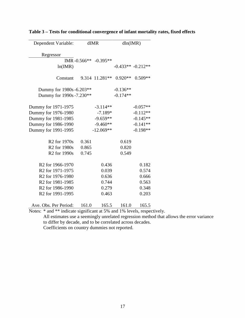
Conditional Convergence – Country Fixed Effects Many of the explanatory variables found in the growth regression literature are similar to, and correlated with, country fixed effects. Variables like distance to the equator, ethnolinguistic diversity, landlockedness, colonial heritage, and region have all been proposed as explanations for countries’ growth rate. All of these variables do not have temporal variation, so a quick way to capture their effect is to simply include country fixed effects in equation (6). Table 3 reports these results, suppressing the coefficients for the country dummies.

These results differ from those in Table 2 in several important ways. First, the regressions in logs now show convergence as well, indicating that even the percentage decline in IMR is larger for higher IMRs, once the country fixed effect is accounted for. Thus, there is no doubt about this conditional convergence. Further, the effect is much stronger, between 8 and 10 percent of initial IMR per year, suggesting that countries converge to their own equilibrium IMR

8 Note that the practice of using lagged values of regressors as instruments is not usually reliable if the concern is that the regressor is endogenous, but that is not the problem here. We simply want to eliminate any bias due to measurement error. As long as the measurement error in period t is uncorrelated with the lagged value of the IMR, this procedure suffices. As it turns out, there is very little difference between these regressions and ones that do not instrument the beginning-of-period IMR.

8

rather quickly. That is also consistent with the low autocorrelations reported in Table 1. Further, the fact that the conditional convergence is so strong, while the absolute convergence is not, suggests that countries do in fact have different equilibrium IMRs. Understanding the reasons for these differences, whether in policies or other country characteristics, thus seems a worthwhile enterprise. Finally, note that the time coefficients are now significantly different from zero, with the largest gains (declines) in the most recent time periods. Thus, once we control for country fixed effects, we have clear evidence of general technical progress in infant mortality rates around the world.

Conditional Convergence – Policy Effects In this section, I explore a variety of policy variables that might have an effect on the rate at which infant mortality declines, conditional on the initial infant mortality rate. The first possibility that I examine is whether the same variables that explain more rapid economic growth also explain more rapid declines in infant mortality. I have already noted that the growth literature has explored scores of variables, too many to try out here. But Table 4 includes five variables that are often significant determinants of economic growth: the black market premium for foreign exchange, a measure of non-market trade restrictions; the ratio of M2 money supply to GDP, a measure of financial depth; the inflation rate, a measure of inefficient taxation; and the real exchange rate, a measure of competitiveness; and the share of children of secondary school age attending school. These variables are all individually and jointly insignificantly different from zero, so there is no evidence that any of these variables helps to explain declines infant mortality. The second regression also includes the log of real GDP per capita (in levels, not its growth), instrumented with the terms of trade, as suggested by Pritchett and Summers (1996). This variable is significant and indicates that, after controlling for the initial IMR, richer countries have more rapid declines in IMR. Doubling GDP per capita causes infant mortality to decline by about 1.5 children per thousand per year. This effect vanishes, however, if we include country fixed effects in the regression (Model 2f). This is perhaps not too surprising, since the level of GDP will change only very slowly and so behave something like a fixed effect. Note that the secondary school variable is statistically significant in three of the four regressions, but with the wrong sign, a result that may be due to its correlation with the real GDP variable or the fixed effects. This result is counterintuitive, and also inconsistent with the growth regression literature, where secondary schooling almost always has a positive impact on growth. Finally, it is interesting that the time dummies change substantially in the fixed effect regressions, becoming progressively more negative and statistically significant. This pattern means that, after controlling for countries’ fixed effects, infant mortality is decreasing at an accelerating rate over time. The next set of regressions considers whether a set of readily available indicators of health care coverage has any effect on declines in infant mortality. In addition to school enrolments, initial IMR, and real GDP per capita, these equations include the number of doctors, nurses, and hospital beds, all per 1000 inhabitants. Model (3) shows that none of the medical care variables is significantly different from zero and, in fact, they all have the wrong sign. Model (4) excludes the number of nurses per 1000 inhabitants because that variable is missing for many countries in the dataset. Excluding that variable increases the sample by a third. Nevertheless, except for the GDP variable, which is now insignificant, the estimates change very

9

little, and neither the number of doctors nor the number of hospital beds has a significant effect on declines in the infant mortality rate. One interesting result from these and almost all regressions that do not include fixed effects is that primary school enrolments significantly increase the rate of decline of infant mortality, but secondary enrolments do not. This result is opposite that usually found in the economic growth literature, where secondary enrolments typically increase growth rates while primary enrolments do not. The fact that the primary enrolment variable becomes insignificant when the fixed effects are included, however, casts doubt on the reliability of the correlation. Like GDP, this variable is unlikely to change rapidly over time, so that it may proxy for some other country characteristic unaccounted for in the regression. Equation (5) includes variables for DPT and measles vaccination rates for infants. These variables do have the correct sign in the regressions without fixed effects, and the DPT rate has a statistically significant, albeit small, effect on the decline of infant mortality rates: a one percent increase in DPT vaccination rates increases the decline in infant mortality by 0.2 children per thousand per year. The (statistically insignificant) effect of measles immunizations is about half of that. Once again, however, including the fixed effects makes these variables insignificant. Another determinant of infant mortality rates that the literature explores is inequality. Waldmann (1992) uses a 57-country cross-section to argue that, after controlling for the level of GDP per capita, a higher share of total income going to the rich increases the infant mortality rate.9 Table 6 explores this possibility with our much larger sample, in a growth regression context. Model (6) includes the gini coefficient, and model (7), which is closer to Waldmann’s specification, includes the share of income going to the richest 20 percent of the population.10 Surprisingly, both regressions suggest that greater inequality increases the rate of decline of infant mortality, contradicting Waldmann. The gini coefficient is not statistically significant, but the richest quintile’s share is. It suggests that an increase in the top quintiles share of 1% causes infant mortality to decline by an extra .13 children per thousand per year. But as with most of the other results, these do not hold up once the fixed effects are included. In addition to the policy variables considered, it is interesting to note that the time dummies are rarely significant and have no clear pattern in the regressions without fixed effects, but they are often significant, and usually decline with time in the regressions with fixed effects. Thus, without accounting for fixed country characteristics, there is no clear trend in the rate of technological progress for infant mortality. This does not imply that things are not improving; they are, but at a rate that is more or less constant over time, not an accelerating one. If we do account for fixed characteristics, then the results suggest significant technological progress in reducing infant mortality after controlling for the other regressors.

9 And of course, there is a burgeoning literature on the effects of inequality on growth of GDP. See, for example, Easterly (2001) or Barro (2000). 10 Waldmann uses the richest 5 percent of the population, but that variable is not on the Deninger and Squire dataset that I use for the distribution data. He also uses the income per capita of the poorest 20 percent rather than national income per capita. The last model in the table uses this variable instead of log(GDP per capita), and yields similar results.

10

Conclusions From the perspective of identifying possible determinants of declines in infant mortality, these results are rather discouraging. Only two policy variables, primary school enrolments and DPT vaccination rates for infants, show any consistent correlation with declining infant mortality, and even those correlations are not robust to the inclusion of fixed effects, a simple way to pick up time invariant unobserved variables.

The other readily available measures of the availability of health care – doctors, nurses, and hospital beds per 1000 inhabitants – have no impact at all on the rate of decline of infant mortality. One could argue that these variables are measured with substantial error, which could account for their low t-statistics (from attenuation bias). But that would not explain why their coefficients are usually positive. It is plausible to suppose that these variables are not too relevant to national infant mortality rates because they measure mostly urban, formal sector health care availability that is not available to most poor people whose children are most at risk. Unfortunately, there are no widely available data on access to the kinds of primary health care that might better explain infant mortality, especially in poorer countries. Perhaps a data collection exercise for health care access and quality similar to the one carried out by Barro and Lee for education is in order.

Perhaps a more interesting “non-result” is the fact that there is no evidence at all that the

black market premium, the M2/GDP ratio, inflation, or the real exchange rate – all policy variables that typically explain economic growth – help to explain declining infant mortality, and only weak evidence that real GDP per capita itself is correlated with these declines. We have long known from microeconomic data that income is not a very good predictor of children’s health status. These results confirm that in a growth regression context. They also suggest that the determinants of progress of nations in one welfare dimension, economic growth, are distinct from those in another, infant mortality.

11

References Barro, Robert J., 2000. “Inequality and Growth in a Panel of Countries,” Journal of Economic

Growth 5: 5-32. Barro, Robert J., and Jong-Wha Lee, 2001. “International data on educational attainment:

updates and implications,” Oxford Economic Papers 53:541-563. Barro, Robert, and Jong-Wha Lee, 1994. “Losers and Winners in Economic Growth,” in

Proceedings of the Annual World Bank Conference on Development Economics, 1993. Barro, Robert, and Xavier Sala-i-Martin, 1999. Economic Growth, Cambridge, MA: MIT Press. Bhargava, Alok, Dean T. Jamison, Lawrence J. Lau, and Christopher J.L. Murray, 2001.

“Modeling the effects of health on economic growth,” Journal of Health Economics 20: 423-440.

Dollar, David, and Aart Kraay, 2001. "Trade, Growth, and Poverty," World Bank Policy

Research Department Working Paper No. 2615. Durlauf, Steven, 2000. “Manifesto for a Growth Econometrics,” Journal of Econometrics

100(1):65-69. Durlauf, Steven, and Danny Quah, 1999. “The New Empirics of Economic Growth,” in John

Taylor and Michael Woodford, Handbook of Macroeconomics, Amsterdam: North Holland.

Easterly, William, “Growth and Life,” Journal of Economic Growth 4(3): 239-76. Easterly, William, 2000. “The Lost Decades: Explaining Developing Countries’ Stagnation

1980-1998,” draft. Easterly, William, and Mirvat Sewadeh, 2001. Global Development Network Growth Database,

http://www.worldbank.org/research/growth/GDNdata.htm. Easterly, William, and Ross Levine, 1997, “Africa’s Growth Tragedy: Polices and Ethnic

Divisions,” Quarterly Journal of Economics 112(4): 1203-50. Granger, C. W. J., and P. Newbold, 1974. “Spurious Regressions in Econometrics,” Journal of Econometrics 2(2): 111-20. Im, Kyung So, M. Hashem Pesaran, and Yongcheol Shin, 1997. “Testing for Unit Roots in

Heterogeneous Panels,” draft.

12

Jones, Charles I., 1995. “Time Series Tests of Endogenous Growth Models,” Quarterly Journal of Economics 110(2): 495-525.

Kormendi, Roger C., and Philip G. Meguire, 1985. “Macroeconomic Determinants of Growth:

Cross-Country Evidence,” Journal of Monetary Economics 16(2): 141-63. Leamer, Edward E., 1983. “Let's Take the Con Out of Econometrics,” American Economic

Review 73(1): 31-43. Levine, Ross, and David Renelt, 1992. “A Sensitivity Analysis of Cross-Country Growth

Regressions,” American Economic Review 82(4): 942-63. Levine, Ross, and Sara Zervos, 1998. “Stock Markets, Banks, and Economic Growth,” American

Economic Review 88(3): 537-58. Macro International, Demographic and Health Surveys, http://www.macroint.com/dhs/. Pritchett, Lant, and Lawrence H. Summers, 1996, “Wealthier is Healthier,” Journal of Human

Resources 31(4):841-868. Scarth, William, 2000. “Growth and Inequality: A Review Article,” Review of Income and

Wealth 46(3): 389-97. Sen, Amartya. 1979. “Personal Utilities and Public Judgment: Or What’s Wrong With Welfare

Economics?” Economic Journal 89:537-58. Sen, Amartya. 1985. Commodities and Capabilities, Amsterdam: North Holland. Sen, Amartya. 1987. “The Standard of Living: Lecture II, Lives and Capabilities,” in The

Standard of Living (Geoffrey Hawthorn, editor) Cambridge: Cambridge University Press, pp. 20-38.

Stifel, David, David Sahn, and Stephen D. Younger, 2000. “Intertemporal Changes in Welfare:

Preliminary Results from Ten African Countries,” CFNPP Working Paper #94.

13

Figure 1 – Infant mortality rates in a cross-section of countries, ordered by rate

0

50

100

150

200

250

0 20 40 60 80 100 120 140 160 180 200

C o u n try

196219801997

14

Figure 2 – Infant mortality rates in a cross-section of countries, ordered by rate

0

1

2

3

4

5

6

0 20 40 60 80 100 120 140 160 180 200

Country

ln(IM

R) 1962

19801997

15

Table 1 – Autocorrelations for the infant mortality rate and its log

Variable: IMR ln(IMR) Ln(Real GDP p.c.) Lag

AC

Partial AC

AC

Partial AC

AC

Partial AC

1 0.416 0.416 0.359 0.359 0.998 0.9982 0.263 0.109 0.228 0.113 0.995 -0.2113 0.122 -0.026 0.107 -0.008 0.991 -0.0904 0.001 -0.080 0.053 -0.006 0.987 -0.0325 -0.260 -0.301 -0.232 -0.300 0.983 -0.0406 -0.268 -0.090 -0.329 -0.227 0.979 -0.0577 -0.344 -0.166 -0.328 -0.129 0.974 -0.0358 -0.137 0.160 -0.158 0.093 0.969 -0.020

16

Table 2 – Tests for absolute convergence of infant mortality rates

Dependent Variable: dIMR dln(IMR)

Regressor IMR -0.111** -0.080**

ln(IMR) 0.081** 0.032**

Constant -9.922** -2.679** -0.691** -0.027**

Dummy for 1980s 2.727 0.050* Dummy for 1990s 8.119* 0.191*

Dummy for 1971-1975 0.205 -0.019Dummy for 1976-1980 -0.942 -0.033*Dummy for 1981-1985 -0.406 -0.022Dummy for 1986-1990 2.102 0.017Dummy for 1991-1995 1.024 0.000

R2 for 1970s 0.162 0.177 R2 for 1980s 0.256 0.088 R2 for 1990s 0.298 0.102

R2 for 1966-1970 0.118 0.010R2 for 1971-1975 -0.024 0.064R2 for 1976-1980 0.235 0.095R2 for 1981-1985 0.288 0.051R2 for 1986-1990 -0.007 0.035R2 for 1991-1995 0.304 0.040

Ave. Obs. Per Period: 161.0 165.5 161.0 165.5

Notes: * and ** indicate significant at 5% and 1% levels, respectively. All estimates use a seemingly unrelated regression method that allows the error variance to differ

by decade, and to be correlated across decades.

17

Table 3 – Tests for conditional convergence of infant mortality rates, fixed effects

Dependent Variable: dIMR dln(IMR)

Regressor IMR -0.566** -0.395**

ln(IMR) -0.433** -0.212**

Constant 9.314 11.281** 0.920** 0.509**

Dummy for 1980s -6.203** -0.136** Dummy for 1990s -7.230** -0.174**

Dummy for 1971-1975 -3.114** -0.057**Dummy for 1976-1980 -7.189* -0.112**Dummy for 1981-1985 -9.659** -0.145**Dummy for 1986-1990 -9.460** -0.141**Dummy for 1991-1995 -12.069** -0.198**

R2 for 1970s 0.361 0.619 R2 for 1980s 0.865 0.820 R2 for 1990s 0.745 0.549

R2 for 1966-1970 0.436 0.182R2 for 1971-1975 0.039 0.574R2 for 1976-1980 0.636 0.666R2 for 1981-1985 0.744 0.563R2 for 1986-1990 0.279 0.348R2 for 1991-1995 0.463 0.203

Ave. Obs. Per Period: 161.0 165.5 161.0 165.5

Notes: * and ** indicate significant at 5% and 1% levels, respectively. All estimates use a seemingly unrelated regression method that allows the error variance to differ by decade, and to be correlated across decades. Coefficients on country dummies not reported.

18

Table 4 – Regressions of change in infant mortality on determinants of economic growth

Model: (1) (2) (1f) (2f) Variable

Intercept -3.635* 8.641 -3.372 -20.311 Black market premium 0.000 0.000 -0.001 0.000

M2/GDP ratio -0.024 -0.033 -0.036 -0.069 Inflation rate -0.003 -0.003 -0.002 -0.001

Real exchange rate -0.006 -0.008* 0.004 0.002 Secondary school enrolment rate 0.028 0.055* 0.133** 0.123**

Beginning of period IMR -0.068** -0.079** -0.195** -0.212** ln(Real GDP per capita) -1.463* 2.185

Dummy for '71-'75 -0.949 -0.984 -2.364* -2.767* Dummy for '76-'80 -0.659 -1.083 -4.688** -5.561** Dummy for '81-'85 -0.788 -1.311 -6.619** -7.610** Dummy for '86-'90 1.794 0.714 -5.991** -6.940** Dummy for '91-95 2.594** 1.695 -6.069** -6.981**

R2, '66-'70 0.333 0.330 0.692 0.686 R2, '71-'75 0.299 0.304 0.491 0.380 R2, '76-'80 0.301 0.306 0.660 0.635 R2, '81-'85 0.363 0.375 0.737 0.737 R2, '86-'90 0.081 0.085 0.487 0.525 R2, '91-95 0.244 0.265 0.434 0.455

Average Observations per Period 75 70 75 70

Notes: * and ** indicate significant at the 5% and 1% levels, respectively. Model is estimated with seemingly unrelated regressions for half-decades. The IMR is instrumented with its own lagged value, and ln(GDP) is instrumented with the terms of trade. A joint test of the black market premium, M2/GDP ratio, inflation rate, and real exchange rate does not reject the null of zero coefficients. Coefficients on the country-specific dummies are not reported.

19

Table 5 – Regressions of change in infant mortality on measures of health care availability

Model: (3) (4) (5) (3f) (4f) (5f) Variable

Intercept 20.411* 13.196* 62.413* 46.461* 4.989 45.745Secondary school enrolment rate 0.020 0.030 -0.060 0.159 0.126* -0.099

Beginning of period IMR -0.105** -0.096** -0.276** -0.219** -0.250** -0.996** ln(Real GDP per capita) -2.075* -1.263 -3.420 -6.015* -0.842 4.234

Primary school enrolment rate -0.081** -0.079** -0.189* -0.027 -0.003 -0.520* Doctors per 1000 people 0.009 0.008 0.002 -0.043 -0.004 0.031 Nurses per 1000 people 0.004 0.001

Hospital beds per 1000 people 0.002 0.002 -0.004 0.007 0.000 -0.031 DPT vaccination rate -0.085* 0.040

Measles vaccination rate -0.046 -0.164 Dummy for '71-'75 -1.918 -0.674 -2.619 -3.099** Dummy for '76-'80 -1.680 -0.804 -4.156* -5.706** Dummy for '81-'85 -0.366 0.310 -2.489 -5.932** Dummy for '86-'90 2.046 2.700 3.778 -2.068 -5.906* -2.472 Dummy for '91-95 -0.510 1.401 2.592 -8.211* -7.220

R2, '66-'70 0.349 0.413 0.515 0.649 R2, '71-'75 0.397 0.321 0.604 0.688 R2, '76-'80 0.396 0.353 0.758 0.770 R2, '81-'85 0.337 0.346 0.734 0.655 0.656 0.823 R2, '86-'90 -0.150 -0.139 -0.004 0.426 0.403 0.921 R2, '91-95 0.274 0.150 0.647 0.195 0.943

Average Observations per Period 44 60 18 44 60 18

Notes: * and ** indicate significant at the 5% and 1% levels, respectively. Model is estimated with seemingly unrelated regressions for half-decades. The IMR is instrumented with its own lagged value, and ln(GDP) is instrumented with the terms of trade. A joint test of the doctors, nurses, hospital beds, and secondary school enrolments does not reject the null of zero coefficients for all these variables in any regression. Coefficients on the country-specific dummies are not reported.

20

Table 6 – Regressions of change in infant mortality on inequality measures

Model: (6) (7) (8) (6f) (7f) Variable

Intercept 0.932 10.830 6.344 22.422 4.064 Secondary school enrolment rate 0.006 -0.015 0.145 0.127*

Beginning of period IMR -0.102** -0.114** -0.072** -0.255** -0.220** ln(Real GDP per capita) 0.848 0.115 -0.204 -2.686 -1.025

Primary school enrolment rate -0.093** -0.079** -0.034* -0.012 Doctors per 1000 people -0.002 -0.002 0.007 0.001

Hosptal beds per 1000 people 0.002 0.002 0.000 -0.003 Gini coefficient -0.039 -0.027

Share of richest quintile -13.386* -18.070** 10.284 Dummy for '71-'75 -0.281 0.486 -0.949 -2.495 -1.626 Dummy for '76-'80 -0.666 0.279 -1.058 -5.017 -3.743 Dummy for '81-'85 0.769 2.196 0.1467 -5.463 -4.048 Dummy for '86-'90 1.119 2.525 0.5625 -5.957 -4.326 Dummy for '91-95 3.252 2.798 1.9756 -7.857 -4.811

R2, '66-'70 0.538 0.535 0.320 0.728 0.856 R2, '71-'75 0.347 0.508 0.436 0.668 0.777 R2, '76-'80 0.468 0.536 0.540 0.853 0.891 R2, '81-'85 0.677 0.714 0.410 0.602 0.378 R2, '86-'90 0.144 0.127 0.223 0.631 0.549 R2, '91-95 -0.241 0.346 0.098 -0.558 -0.083

Average Observations per Period 40 32 55 39 32

Notes: * and ** indicate significant at the 5% and 1% levels, respectively. Model is estimated with seemingly unrelated regressions for half-decades. The IMR is instrumented with its own lagged value, and ln(GDP) is instrumented with the terms of trade. Coefficients on the country-specific dummies are not reported.