Cross-Layer Flow and Congestion Controlfor Datacenter Networks

(Invited Paper)

Andreea S. Anghel, Robert Birke, Daniel Crisan and Mitchell GusatIBM Research, Zürich Research Laboratory

Säumerstrasse 4, CH-8803 Rüschlikon, Switzerland

{aan,bir,dcr,mig}@zurich.ibm.com

Abstract—A key feature of the upcoming datacenter networksis their losslessness, achieved by the means of Priority FlowControl (PFC). Inherited from the cluster and HPC networksthat traditionally use link level flow control to prevent packet lossacross multiple virtual lanes, channels and/or priorities, this fea-ture is now also becoming widely available in the next generation10, 40 and 100Gbps Ethernet switches and adapters. Nevertheless,excepting storage protocols such as Fibre Channel over Ethernet,PFC is new and unfamiliar to the majority of datacenterapplications and protocols. That is, despite PFC’s key role in thedatacenter and its increasing availability – supported by virtuallyall future Converged Enhanced Ethernet (CEE) products – itsimpact on the higher layer routing and transport protocolshas yet to be investigated. Hence our motivation to assess theperformance exposure of three widespread TCP versions to PFC,as well as to the potentially conflicting Quantized CongestionNotification (QCN) congestion management mechanism, whichapparently replicates on Layer 2 some more advanced TCPfunctionality.

As workloads of interest we have selected a few revealingcommercial and scientific applications. For quantitative per-formance evaluation we use two distinct methodologies: (a)Our reference is an accurate Layer 2 CEE 10Gbps networksimulator intercoupled with TCP implementations extracted fromFreeBSD v9; (b) A hardware setup scaled down in speed andsize. The main outcome of our work is that PFC can notablyimprove the TCP performance across all tested configurationsand workloads. This result was validated in both environments.Hence our recommendation to enable PFC whenever this ispossible. By contrast, QCN can either harm or help dependingon its parameter settings, and essentially, on the co-existence ofcompeting UDP or other non-congestion-managed traffic.

I. INTRODUCTION AND MOTIVATION

Ethernet was originally designed to be a simple and inex-

pensive Plug-and-Play LAN solution. Nonetheless, it was not

optimized for performance i.e. low latency, high throughput,

traffic differentiation, low packet loss ratio. In order to fill

the gap, HPC and datacenter architects have built specialized

networks such as, Infiniband, Myrinet, Fibre Channel etc.

While outperforming the low cost Ethernet, this specialized

multiple network infrastructure is expensive to build and

difficult to maintain. As a consequence, in order to save

overhead, power and cost, a better solution was to converge

all the datacenter traffic in one single consolidated network,

i.e. Converged Enhanced Ethernet (CEE) datacenter network.

One of the CEE key features is Layer 2 (L2) losslessness.

This is achieved via per priority link-level flow control as

defined by 802.1Qbb PFC [1]. However, the benefits of

losslessness via PFC are not free of side effects. Besides the

potential for multiple types of deadlocks in various common

topologies and switch architectures, any stiff link level flow

control may lead to saturation tree congestion, oscillations

and critical instabilities. To counteract the potentially severe

performance degradation due to such undesirable phenomena,

IEEE has recently standardized a new L2 congestion control

scheme capable to deal with sustainable network congestion,

Quantized Congestion Notification (QCN, 802.1Qau) [2].

Future CEE datacenter networks will have to manage up

to one million physical – and 20-300x more virtual – nodes

connected in a single L2 domain via multipathing across 10-

100 Gbps links of at most a few 10s of meters. The round-

trip times (RTT) range from 0.5 μs up to a few tens of μs,

except under hotspot congestion, when the end-to-end delays

can grow by several orders of magnitude, reaching into 10s

of ms or more[3]. However, even if a congested DCN may

have RTTs similar in magnitude with a WAN, there is a key

difference. Unlike the wide area networks where the RTT

is mostly due to flight delays, in datacenter environments

the network RTT is dominated by queuing delays, which

under bursty workloads [4], [5], [6], [7], [8], [9], [10], [11],

lead to a difficult traffic engineering and control problem.

Hence the recent surge in research and standardization efforts

addressing the new challenges in datacenter virtualization,

flow and congestion control, routing and high performance

transports.

Apart from enabling the convergence of legacy and future

datacenter applications, CEE datacenter networks must also

meet the QoS requirements of a wide variety of applications

such as business analytics, algorithmic trading, large scale Web

services, cloud services (storage, computation), multimedia

streaming, MPI workloads etc. These applications generate

traffic with specific communication patterns. The bulk of

the datacenter communications remains based on Layer 4

(L4) transport protocols, mostly TCP - with some notable

exceptions such as UDP, SCTP or RDMA. In this paper we

study the impact of the new CEE features on the typical

datacenter applications performance. We focus on analyzing

TCP commercial workloads that generate scatter/gather com-

44978-0-9836283-2-3 c© 2011 ITC

This paper was peer reviewed by subject matter experts for publication in the Proceedings of DC–CaVES 2011

Figure 1. QCN Congestion Detection – Load Sensor at Congestion Point:It is implemented at the switch buffer level by monitoring the output queues.Its main objective is to keep the buffer occupancy at a certain level Qeq .Algorithm: The QCN load sensor is sampling the input frames based onthe probability function in 1. For each sampled frame, the load sensormeasures the current queue occupancy level (Qlen) and computes the queueoccupancy excess (Qoffset = Qeq−Qlen), the queue rate excess (Qdelta =Qold −Qlen) and the feedback value (Fb = Qoffset +w ·Qdelta). Qold

is the occupancy level at the previous sample and Qeq is the target queueequilibrium (setpoint). If the computed feedback is negative a 64 B congestionnotification message (CNM) frame, including a 6-bit hotspot severity value(feedback), is sent back directly to the source of the sampled frame.

munication patterns –aka, Partition/Aggregate– as described in

[4], [6].Assuming that TCP will continue as the paramount transport

for the foreseable future, we ask three TCP-related questions:

(Q1) How does TCP perform over CEE networks - does it

work ’out of the box’, or is tuning/adaption necessary? (Q2) Is

PFC, with its correlated multiple hotspots and saturation trees,

beneficial, neutral or detrimental to TCP, which traditionally

has relied on loss as congestion feedback from uncorrelated

single bottlenecks? (Q3) Is QCN’s TCP-like L2 rate control

beneficial, neutral or detrimental to TCP? By addressing these

questions we hope to provide some useful insight to datacenter

architects, network vendors, as well as operating system,

hypervisor and application designers.Our contributions are twofold, structured as follows.Methodology: We use two evaluation methodologies pre-

sented in SECTION III and SECTION IV corresponding to: (i).

simulation environment; (ii). hardware setup.In the simulation environment: (i). In SECTION III-B we

explain the network models including the necessary parameter

changes for TCP over 10 Gbps CEE; (ii). As benchmark

applications, we have adopted three datacenter workloads,

including commercial workloads (see SECTION III-C); (ii). At

Layer 4, we extracted three TCP versions from FreeBSD v9,

each representing a different class of TCP implementations,

and ported them to our simulation environment: New Reno,

Vegas and Cubic; (iii). At Layer 2, we instrumented our

simulator with PFC and QCN. For performance evaluation we

have mixed hardware and software experiments with detailed

Figure 2. QCN Rate Limiter (RL) – Rate Control at Reaction Point: Uponreceiving a CNM, a QCN-compliant source reacts by instantiating a ratelimiter (RL) and setting the Target Rate (TR) to the Current Rate (CR). CRis the RL TX rate at any instant of time while TR is the RL TX rate justbefore the reception of a CNM. After that it adjusts its TX rate based on anAIMD-like strategy. Algorithm: Upon reception of a CNM, the RL reducesCR to CR = CR ∗ (1 − G ∗ |Fb|). The higher the feedback value, thehigher the rate reduction according to the rate decrease control law. The rateincrease is performed in 3 phases: Fast Recovery (FR), Active Increase (AI)and HyperActive Increase (HAI). For each CNM received, the source resetsa byte counter and enters the Fast Recovery phase to autonomously recoverthe lost TX rate. FR has 5 cycles (from C1 to C5), each of them consisting of150 KB transmitted by the RL. At the end of a cycle, the RL CR is updatedto CR = 1/2 ∗ (CR + TR). After 5 cycles in FR, the RL enters the AIphase. In this phase, the RL counts cycles of 75 KB each. At the end ofa cycle, the target rate is updated to TR = TR + R where R is 5 Mpbs

and the current rate to CR = 1/2 ∗ (CR + TR). The byte counter is usedsimultaneously with a timer. They are executed independently, but they jointlydetermine the rate increase of the RL. The timer was introduced to speed-upthe rate recovery especially when the RL current rates at the moment of aCNM reception, are small. Upon reception of a feedback message, the timeris reset and the RL enters the FR phase. It counts 5 cycles of T = 10 ms

duration, and then enters the AI phase where each cycle is T/2 = 5 ms

long. In each of the two phases, FR and AI, a cycle ends when either a bytecounter or a timer completes its cycle. When both the timer and the bytecounter are in the Active Increase phase, the RL is in the HAI phase. If theRL succeded to enter this phase, the network condition is considered stableand the probability for the RL to cause network congestion is small. Thus,CR and its corresponding RT have a higher growth rate: TR grows in stepsof 50 Mbps and CR accordingly to the same increase law as in the AI phase.

L2 simulation models of CEE switches and adapters.

In the hardware environment: (i). In SECTION IV we present

the network models including the necessary parameter changes

for TCP over FastEthernet networks; (ii). As benchmark appli-

cations, we implemented a version of commercial workloads;

(ii). At Layer 4, we use three TCP modules already present

in Linux Kernel 2.6.32 for New Reno, Vegas and Cubic; (iii).

At Layer 2, we use PFC with one priority only (i.e. 802.3x

PAUSE).

Results: In both SECTION V and SECTION VI we present

evidence of PFC’s benefits to TCP performance, leading to

our recommendation to enable PFC also for TCP applications.

The hardware testbed validates the PFC results obtained in the

simulation environment. With respect to QCN, we identify

cases in which it is beneficial, repectively detrimental to

Proceedings of the 2011 3rd Workshop on Data Center — Converged and Virtual Ethernet Switching 45

L4 TCP (Reno) L2 QCN

DETECTION MECHANISM

- Implemented (1) at the destination (duplicate ACK); (2) in the network atthe congestion point (AQM/ECN); (3). at the source (RTO)(1) For each packet loss the destination will ask the sender for retransmissionby sending it a duplicate ACK. Upon reception of 3 duplicate ACKs, thesource enters the fast recovery phase.(2) When an ECN packet arrives at a RED-enabled congested queue, therouter may mark the packet instead of dropping it.(3) The RTO value is set larger than the maximum RTT value of the network.A packet loss can imply an RTO and then TCP enters the slow start settingthe congestion window at 1 MSS.

- Implemented at the congestion point in the network.- It monitors the L2 queues and in the event of congestion it sends a CNMto the culprit source node.- The congestion point sensor randomly samples with a variable samplingprobability the queue characterized by two state variables, position andvelocity, defined with respect to a pre-established set-point Qeq . Based onthe queue size and velocity values, the CP evaluates the level of congestionby computing a congestion feedback. If negative, a CNM is sent back to theculprit of the sampled frame.

FEEDBACK TYPE

Duplicate ACKECN/RED single bit feedbackRetransmission Time-out

If the feedback computed is negative, it is quantized on 6 bits (multibit).

BURST TOLERANCE

Tolerant to bursts The value of the setpoint Qeq determines how tolerant QCN is to burstytraffic, but overall QCN is less tolerant than established L4 CM schemes.

TIMESCALE

100s of ms. Depends on network RTT and default RTO. 10s to 100s μs

Table ICONGESTION DETECTION

L4 transports. The QCN performance proves to be highly

dependent on the type of workload and its generated com-

munication pattern. The same remark applies for ECN-RED:

the simulation results show either benefit or detriment to TCP

performance.

The rest of the paper is organized as follows. The CEE

datacenter network stack is described in SECTION II. In

SECTION III we present the simulation environment, the

network models, the workloads used in our evaluation and the

performance metrics. In SECTION IV we explain the hardware

experimental setup, the corresponding network topology and

the applications used for the hardware evaluation. In SECTION

V we present simulation results and discuss their implications.

The results obtained in the hardware testbed are shown in

SECTION VI. Related work is presented in SECTION VII, after

which we conclude in SECTION VIII.

II. DATACENTER NETWORK STACK

A. Layer 2 - Converged Enhanced Ethernet (CEE)

There is a growing interest in consolidated network solu-

tions that meet the requirements of datacenter applications,

i.e., low latency, no loss, burst tolerance, energy efficiency.

One possible answer to the universal datacenter fabric is CEE

with the following key features: (i) per-priority link-level flow-

control and traffic differentiation, i.e., Priority Flow Control

(PFC; IEEE 802.1Qbb) [1]; (ii) congestion management, i.e.,

Quantized Congestion Notification (QCN, optional in CEE;

IEEE 802.1Qau) [2]; (iii) transmission scheduling: Enhanced

Transmission Selection (ETS; IEEE 802.1Qaz).

1) PFC: Conventional IEEE 802.3 Ethernet does not pro-

vide reliability. Indeed, whenever a network device buffer

reaches its maximum capacity, packets are dropped. Upper

layer protocols such as TCP rely on these events and interpret

them as congestion feedback, thus triggering window or rate

adjustments. This goes against the strict QoS requirements of

many of the nowadays datacenter applications such as FCoE,

MPI or Business Analytics.

A mechanism that can avoid packet losses is IEEE 802.3x

PAUSE [1]. This protocol pauses the transmitter side of an

Ethernet link whenever the receiver side buffer occupancy

exceeds a maximum threshold by means of explicit PAUSE

XOFF control frames. The transmission resumes once a time-

out expires or a PAUSE XON control frame is received. The

PAUSE XON frames are produced when the occupancy falls

below a given minimum threshold.

Two main drawbacks affect this solution: (i) no knowledge

of service classes: pausing a link due to one application will

affect all applications using that link; (ii) possible throughput

collapses: if a sender is blocked, its buffer may get filled up

and recursively other network devices will possibly get paused

and will fill up as well, creating congestion spreading and thus

a congestion tree which will drastically decrease the network

throughput.

PFC addresses both by dividing the traffic into 8 different

priorities based on the IEEE 802.1p class of service field.

Inside each priority PFC acts exactly as 802.3x PAUSE, but

one priority does not affect the others. This addresses directly

drawback (i) and reduces the probability of drawback (ii).

However, incorrectly implemented, PFC can still generate

switch memory-to-memory (M2M) circular dependency and

routing deadlocks. Routing deadlocks can be avoided using

a loop-free topology such as fat-tree topologies [12]. M2Ms

are a more general issue and happen due to un-ordered access

to mutually blocking resources. For instance if two shared-

46 Proceedings of the 2011 3rd Workshop on Data Center — Converged and Virtual Ethernet Switching

L4 TCP (Reno) L2 QCN

PRINCIPLE OF OPERATION

- Implemented at the source - Window Controller.- It uses a congestion window for controlling the injection rate.

- Implemented at the source - Rate-based Controller.- It uses a Finite State Machine (based on a byte counter and a timer) and aCubic like algorithm.

INCREASE/DECREASE RATE CONTROL LAW

Additive Increase (AI) - Multiplicative Decrease (MD)- A time-out reduces the current congestion window at 1 MSS and TCP entersthe Slow Start phase. Three duplicate ACKs halve the TX congestion window,which is the standard TCP decrease law according to MD.- The TX rate is recovered slowly (the duration is in the range of multipliersof RTT).- The TX rate recovery phase is RTT-dependent.

Fast Recovery - Active Increase - Hyper Active Increase (Cyclic like)- The reception of a CNM reduces the TX rate by a variable amountproportional to the feedback magnitude, up to maximum 50 percent of theCR.- For a reference, 10 Gbps CEE with a singular maximum rate reduction(downto CR/2), the CR/2 rate ’drop’ can be recovered in min. 770 μs.- The TX rate recovery control phase is RTT-independent (unlike CUBIC,QCN does not exhibit RTT-based self-clocking).

Table IICONGESTION CONTROL

memory switches A and B exceed their thresholds and if all

the traffic from A is destined to B and vice-versa, neither

can send. This deadlock can be overcome by partitioning the

switch memory and enforcing the thresholds on a per input

basis.

2) QCN: QCN is an L2 congestion management technique

that provides a set of mechanisms for controlling the network

congestion generated by long-lived data flows. QCN detects

congestion, reports it via explicit congestion feedback and

adapts the source node injection rate to the available network

capacity. QCN accomplishes these two steps by using two

distinct algorithms.

One is the QCN load sensor mechanism which is im-

plemented at the Congestion Point (CP) in the network.

Its objective is to monitor the queues and, in the event of

congestion, send a notification to the culprit source node.

The congestion point sensor randomly samples with a variable

sampling probability Ps the queue characterized by two state

variables, position and velocity {q, q′}, defined with respect

to a pre-established setpoint Qeq . The algorithm is explained

in FIGURE 1.

The second algorithm is implemented at the Reaction Point

(RP) (i.e. source node). It is called the QCN Rate Limiter

and reacts to the congestion signals by reducing/increasing the

transmission rate according to the feedback received from the

CP. This algorithm uses a byte counter and a timer. FIGURE

2 shows how the RP algorithm adjusts the injection rate.

B. Layer 3 - ECN - RED

Random Early Detection (RED) is an L3 Active Queue

Management (AQM) congestion avoidance technique for

packet-switched networks. Unlike QCN whose congestion

estimation is based on instantaneous queue size measure-

ments, RED detects network congestion by computing the

average queue length and comparing it with a given threshold.

The RED-enabled queue has a minimum and a maximum

threshold. If the average queue length is below the minimum

threshold, all incoming packets are forwarded unchanged. If

the average queue length is above the maximum threshold,

all the incoming packets are dropped. Finally, if the average

queue length is between the threshold values, some of the

incoming packets are dropped according to a liniar probability

which is function of the average queue length. Out of the

remaining packets, the ones that are ECN capable are marked

[13]. An important advantage of using this mechanism is that

by monitoring the queue and by keeping its length small,

RED allows the network to absorb a limited amount of bursty

traffic with little performance degradation. Unlike the QCN

load sensor mechanism, RED is more tolerant to bursts as

confirmed later in the paper.

Proceedings of the 2011 3rd Workshop on Data Center — Converged and Virtual Ethernet Switching 47

Explicit Congestion Notification (ECN) is a L3-L4 end-to-

end congestion management protocol defined in RFC 3168.

The principle of this protocol is for the transmission node

to receive network congestion notifications without the need

for any packets to be dropped. In order to be operational and

efficiently used, ECN has to be supported by both endpoints

and also by the intermediate network devices.ECN uses the two least significant bits of the Differential

Services (DiffServ) field in the IP header. Once the commu-

nicating nodes have negociated ECN, the transport layer of

the source node sets the ECN codepoint in the IP header

of the packet and sends the packet to the destination. When

the ECN-capable packet arrives at a RED-enabled queue that

is experiencing a congestion, the router may decide to mark

the packet instead of dropping it. Upon receiving the marked

packet, the destination sends back to the transmission node an

ACK packet with the ECN-Echo bit set. This way the transmis-

sion node receives a signal to reduce its transmission rate. The

destination repeats sending ACK packets until the transmission

node acknowledges having received the congestion indication.

C. Layer 4 - TCP Versions

We have selected three representative TCP versions:

1) TCP New Reno [14] since it is both the best known and

the most implemented one;

2) TCP Cubic [15] since it is the standard implementation

in today’s Linux kernels;

3) TCP Vegas [16] since it uses a distinct congestion

control scheme than the others two i.e. delay-probing

instead of loss-based congestion window adjustment.

TCP New Reno, like Reno, includes the slow-start, congestion

avoidance, fast retransmit and fast recovery algorithms. Its

congestion feedback is either packet loss and/or ECN-marked

packets. TCP New Reno outperforms TCP Reno in the pres-

ence of multiple holes in the sequence space, but performs

worse in case of reordering due to useless retransmissions. It

was the standard TCP implementation in Linux kernels till

version 2.6.8.TCP Cubic is RTT-independent. It has been optimized for

high speed networks with high latency (due to flight delays)

and is a less aggressive derivative of TCP BIC (Binary Increase

Congestion control). TCP BIC uses a binary search to probe

the maximum congestion window size. TCP Cubic replaces

the binary search with a cubic function. The concave region

of the function is used to quickly recover bandwidth after a

congestion event happened, while the convex part is used to

probe for more bandwidth, slowly at first and then very rapidly.

The time spent in the plateau between the concave and convex

regions allows the network to stabilize before TCP Cubic starts

looking for more bandwidth. TCP Cubic replaced TCP BIC

as the standard TCP implementation in Linux kernels from

version 2.6.19 onwards.While both TCP New Reno and TCP Cubic rely on losses

to detect congestions and react accordingly, Vegas avoids con-

gestion by comparing the expected throughput in the absence

of congestion with the actual achieved throughput and then it

Figure 3. Two-tiered datacenter network topology with edge and aggregationswitches and 64 end-nodes distributed in 4 racks. This topology is anXGFT(2;16,4;1,2). The 16 external query sources are acting as the HLAsfor the scatter/gather communication pattern generated by the application.These external sources inject TCP queries in the datacenter network throughthe Level 2 aggregation switches.

adjusts the transmitter window size accordingly. TCP Vegas is

representative for the delay-probing class of TCPs similar to

Adaptive Reno and Compund TCP.

Table I shows a qualitative comparison between TCP and

QCN with respect to the congestion detection mechanism.

Table II shows a similar comparison but with regard to the

congestion control scheme.

III. EVALUATION METHODOLOGY I: SIMULATION

ENVIRONMENT, MODELS, WORKLOADS

A. Simulation Environment

A network simulation environment brings a set of clear

advantages against the hardware experiments: (1). It gives

access to a detailed overview of the behavior and interaction

of different network protocols which may be unavailable on

hardware equipments; (2). The scalability of the protocols

can be tested with large-scale scenarios and configurations;

(3). The protocols and the system design parameters can be

easily modified in order to find the optimal system configu-

ration which delivers the best performance results; (4). The

experiments results can be easily replicated. On the other

hand, there are deficiencies that have to be corrected in the

case of a network simulation environment. The most relevant

drawback is that it is difficult to integrate all the details from

real environments and create realistic models for all the L2-

L4 protocols and datacenter network components. Hence, for

our simulations we chose to calibrate the simulation models

by using hardware experiments. However, apart from the

simulation environment, we also propose and test a hardware

setup described in IV.

Even though there are already well established network

simulation tools in the community such as NS-3 which has

a large library of supported L3/L4 protocols, we chose not to

use NS-3, but our own network simulation enviroment based

on Omnet++ for the following reasons: (1). It has support for

CEE standards including PFC, QCN and ETS; (2). It contains

management and monitoring for the L2 queues and buffers, L2

scheduling, link-level flow control and memory management

48 Proceedings of the 2011 3rd Workshop on Data Center — Converged and Virtual Ethernet Switching

(a) TX Stack Delay. (b) RX Stack Delay.

Figure 4. (a): The TX delay is measured as follows: the UDP traffic generator application adds a timestamp (T1) to the payload of the packet right beforewriting the packet to the L4 socket buffer (step 1); the driver adds a timestamp (T2) just before queuing the packet onto the TX ring buffer (a shared bufferbetween the driver and the NIC hardware) (step 4); the TX delay is computed as the difference between these two timestamps (T2-T1). (b): The RX delayis measured as follows: the driver adds a timestamp (T3) to the payload of the packet that it receives from the RX ring buffer (again the same shared bufferbetween the driver and the NIC hardware) (step 4); the application adds a timestamp (T4) to the payload of the packet just after reading the packet from theL4 socket buffer (step 7); the RX delay is computed as the difference between these two timestamps (T3-T4).

at both switch and adapter micro-architecture level; (3). L4

protocols are ported from the BSD, AIX and Linux kernels

and they are more complex than the TCP libraries in NS-

3 which trade accuracy for simulation efficiency. Based on

these features, our simulation environment is able to analyze

the interaction between the L4 and L2 protocols. Our platform

entails two simulators coupled in an end-to-end framework,

Dimemas and Venus [17] and the TCP simulations are real-

istically calibrated against the actual OS stacks running on

hardware.

B. Network Models

1) Datacenter Topologies: A widely used topology for data

center networks is the fat tree topology. A fat tree can be

described as a multi-stage tree topology where the bandwidth

of the connections increases towards the root of the tree [18].

The network topologies used in our simulations belong to the

family of extended generalized fat trees (XGFT) [12] which

is a more general formalization of fat trees. This family also

includes other popular data center interconnection networks,

such as k-ary n-trees and slimmed k-ary n-trees. An XGFT

(h;m1, ...mh;w1, ...wh) has h+1 levels of nodes divided into

leaf nodes and inner nodes. There are∏h

i=1mi leaf nodes

occupying level 0 and they serve as end nodes/servers. The

inner nodes occupy levels 1 to h and serve as switches. Each

non-leaf node on level i has mi child nodes and each non-root

node on level j has wj+1 parent nodes.

For commercial workload evaluations we use two prac-

tical, albeit scaled down in size, XGFT topologies:

XGFT(2;32,4;1,2) and XGFT(2;16,4;1,2). The latter is shown

in FIGURE 3. In the first scenario, described in SECTION V-B,

we use the XGFT(2;16,4;1,2) topology and we inject only TCP

traffic in the network. In the second scenario, mentioned in

SECTION V-C, we inject both TCP and UDP traffic, but we

use the XGFT(2;32,4;1,2) network topology.

For the MPI workloads using scientific application traffic we

use two slightly different topologies: XGFT(2;16,7;1,2) and

XGFT(2;32,7;1,2).

2) TCP Transport Model: According to [19] TCP computes

the RTO value based on two variables: a smoothed round-trip

time average (SRTT) and an average RTT variance (RTTvar).

The RTT of a packet is measured as the interval between

sending a segment and receiving its corresponding ACK.

Initially, when a first RTT measurement RTT 1 is made,

SRTT 1 = RTT 1, RTT 1var = RTT 1/2 and RTO1 =

SRTT 1+max(G,K ∗RTT 1var), where K was originally set

to 4, and G is the clock granularity in seconds. For the next

RTT measurements, SRTTN and RTTNvar are calculated as

follows: RTTNvar = (1 − a) ∗ RTTN−1

var + a ∗ |SRTTN−1 −RTTN | and SRTTN = (1 − b) ∗ SRTTN−1 + b ∗ RTTN

where 0 ≤ a < 1 and 0 ≤ b < 1. Once the source has

computed these values, it will update the RTO according to

RTON = SRTTN +max(G,K ∗RTTNvar) (Eq. 1).

In order to realistically model the TCP transport protocol,

we ported the TCP stack from the FreeBSD v9 kernel in

our simulation environment. Further calibration was needed to

adapt the TCP parameters to the actual network characteristics.

Thus we changed three parameters: (1) the CPU clock tick rate

of the system; (2) the RTO default values and, (3) the RTO

variance. Similar changes will be considered for the hardware

testbed in IV.

(1) CPU clock tick rate: In our simulations we use a network

with 10 Gbps links. Given this and the topology, the RTT of

the network is small, in the range of tens of microseconds.

The kernel timer quanta is set by default at 1 ms. By using

this default coarse-grain kernel timer, the RTT measurements

cannot be accurate. The accuracy of the RTT estimation is

critical especially for delay-probing TCP protocols such as

Proceedings of the 2011 3rd Workshop on Data Center — Converged and Virtual Ethernet Switching 49

Vegas and Compound TCP [20]. Compared to Cubic and New

Reno which react to congestion upon packet loss, TCP Vegas

detects congestion by comparing the measured throughput

with an expected one, whose computation is RTT-dependent.

Thus, TCP Vegas relies on fine resolution timers for obtaining

accurate timing information to compute the actual and the

expected throughputs, and to accordingly adjust its congestion

window. As a consequence we increased the timer granularity

from 1 ms to 1 μs. A higher gramularity time also contributes

to correctly compute the RTO value (see Eq. 1).

(2) Default RTO values: In addition to the CPU clock tick

rate calibration, we also had to adapt the default RTO value

to the actual RTT value of the network. Based on our network

measurements and [10], [7], we reduced the value of the

minimum RTO to 2 ms. The kernel default value for the RTO

value was 3 s. We reduced the default RTO to 10 ms, larger

than the maximum RTT of our network, so that we could avoid

the Flow Completion Time (FCT) to be drastically penalized

by a SYN packet loss when PFC is disabled.

(3) RTO variance: The retransmission time-out is computed

by using the Van Jacobson’s timer estimator which takes into

account the variance measured in the RTT values. A constant

term is added to the estimation, accounting for the variance in

segment processing at the end-point kernels. Hence, in order

to match the current fast processors, we also modified the term

K in Eq. 1, from the default FreeBSD value of 200 ms to 20

ms.

Nevertheless, by porting TCP to our simulation environ-

ment, we had to perform some other optimizations. Some

of them are related to the allocation and deallocation of

segments. Others are: (1). Connection TCP parameter cache:

the congestion window and the RTT estimation are inherited

from the previous connection; (2). Adaptive TCP buffers: the

TCP buffers sizes are dynamically modified in response to an

RTT change.

3) TCP Stack Delay Evaluation: When a packet is sent

from an application, it is first written to a TCP send buffer

and copied to the kernel memory. Then it is pushed to the IP

layer and, if the transmission queue tx_qdisc is not full, it is

succesfully enqueued. After that the driver removes the packet

from the tx_qdisc and maps it into the transmission descriptor

ring buffer called tx_ring. Finally, if resources are available,

the NIC consumes the packet from the tx_ring, copies it to its

memory using DMA and sends it out on the wire.

When a packet is received, the NIC transfers the packet via

DMA into a free descriptor taken from the reception descriptor

ring buffer called rx_ring. Once fully transfered an interrupt is

raised to signal the new packet to the device driver. The device

driver takes the packet out of the rx_ring and sends it to the

network stack. In order to reduce the system overhead, while

being processed by the upper layers, the packet remains in

kernel memory. The packet is first consumed by the IP layer

and then, if it is a TCP packet, it is forwarded to the TCP

receive process. Finally the packet is eventually consumed by

the application.

We determined the delay of the TCP stack by modifying

Table IIISIMULATION NETWORK PARAMETERS

Parameter Value Unit Parameter Value Unit

TCP Other

buffer size 128 KB TX delay 9.5 μs

max buffer size 256 KB RX delay 24 μs

default RTO 10 ms timer quanta 1 μs

min RTO 2 ms reassembly queue 200 seg.

RTO variance 20 ms

ECN-RED

min thresh. 25.6 KB Wq 0.002

max thresh. 76.8 KB Pmax 0.02

QCN

Qeq 20 or 66 KB fast recovery thresh. 5

Wd 2 min. rate 100 Kb/s

Gd 0.5 active incr. 5 Mb/s

CM timer 15 ms hyperactive incr. 50 Mb/s

sample interval 150 KB min decr. factor 0.5

byte count limit 150 KB extra fast recovery enabled

PFC

min thresh. 80 KB max thresh. 97 KB

Network hardware

link speed 10 Gb/s adapter delay 500 ns

frame size 1500 B switch buffer size/port 100 KB

adapter buffer size 512 KB switch delay 100 ns

a Linux 2.6.32.24 kernel running on an Intel i5 @ 3.2GHz

machine with 4 GB of memory. We instrumented the E1000e

Ethernet device driver of an Intel 82578DM Gigabit Ethernet

controller. The stack delay was measured both in transmission

and reception. The transmission delay was measured as the

time spent between the application sending the packet and the

moment the packet being enqueued in the tx_ring. Similarly,

the reception delay was measured as the time spent from

the moment a frame being ataken out of the rx_ring and

the application receiving the data. Unfortunately the delay

introduced by the NIC hardware operations is not measurable

from software. For details see FIGURE 4. The average values

are reported in TABLE III and the probability distributions are

shown in FIGURE 5.

4) Simulation Network Parameters: The network link speed

is 10 Gbps. In accordance with the 802 Data Center Bridging

reference switch model, we have assumed a canonical ideal

input buffered (IB), output queued (OQ) switch with 100

KB per input buffer. While both of the PFC thresholds are

defined with regard to this input buffer, the QCN setpoint is

defined with respect to the output queues. Practically, however,

such an OQ is emulated by the means of input buffered (IB)

and crossbar hardware switches, which may not provide a

dedicated hardware OQ - which was the key element for L2

QCN (the QCN algorithm implemented is based on version

2.4 [2]). In addition, our switch has N input buffers and the

write bandwidth into an OQ is equal to N times the line rate.

The size of an OQ is bounded only by the sum of all the input

buffers for all ports. However this is not true in reality, because

a single output queue can not monopolize the full memory.

In addition, each input adapter provides one virtual output

queue (VOQ) for each destination. This avoids most of the

head-of-line blocking, which can be further exacerbated by

the QCN rate limiters. TABLE III contains the key parameters

50 Proceedings of the 2011 3rd Workshop on Data Center — Converged and Virtual Ethernet Switching

0

10

20

30

40

50

60

0 5 10 15 20 25 30 35 40

PDF

[%]

Delay [us]

NoneUDP srcUDP dst

TCP

(a) TX stack delay PDF.

0

0.1

0.2

0.3

0.4

0.5

0.6

0.7

0.8

0.9

1

0 5 10 15 20 25 30 35 40

CD

F

Delay [us]

NoneUDP srcUDP dst

TCP

(b) TX stack delay CDF.

0

2

4

6

8

10

12

14

16

18

20

0 5 10 15 20 25 30 35 40

PDF

[%]

Delay [us]

NoneUDP srcUDP dst

TCP

(c) RX stack delay PDF.

0

0.1

0.2

0.3

0.4

0.5

0.6

0.7

0.8

0.9

1

0 5 10 15 20 25 30 35 40

CD

F

Delay [us]

NoneUDP srcUDP dst

TCP

(d) RX stack delay CDF.

Figure 5. Linux 2.6.32.24 Kernel Stack Delay Results

of the network.

C. Applications, Workloads and Traffic

As stated at the onset, we aim to evaluate the impact of

different L2, L3 and L4 protocols on performance at the

application level, centered on revealing the TCP sensitivities

to the two new CEE features: PFC and QCN. Therefore we

have selected a few key datacenter applications, divided in two

groups: commercial and scientific workloads.1) Commercial Applications: For evaluation we focus on

commercial workloads that generate the scatter/gather (parti-

tion/aggregate) traffic communication pattern. This pattern is

currently used by many large scale web applications such as

web search or social networking applications. The traffic study

from [4] confirms this finding. In addition, scatter/gather is a

good candidate to analyze the challenges that TCP has to deal

with in current datacenter networks.The principle of operation of this communication pattern

is as follows: (1). A central process receives a query/request

(i.e. a web search request); (2). It divides the query into

subqueries (i.e. parts from the web search index) and sends

them to multiple workers (scatter phase); (3). The responses

from the workers are collected by an aggregator (gather

phase); (4). The aggregator merges the responses into a single

response message which is sent back to the source of the

query. This process might repeat on the workers in the sense

that a certain worker might further segment the subquery

and dispatch the segments to a second layer of workers. We

obtain thus several layers of scatter of queries and gather of

responses. In order to meet the latency requirements of the

user application, the workers are assigned tight deadlines to

provide the answer to the query. However, TCP can prevent

the workers from meeting the deadlines thus reducing the

relevance of the final response. Moreover, the gather phase

of the pattern is intrisically prone to generating bursty traffic

thus increasing the probability to produce network congestion

and lose packets. Depending on what L4 congestion control

scheme it is used at the end nodes, packet loss can increase

dramatically the flow completion time.

In our simulations we use a three level scatter/gather

pattern. The High Level Aggregators (HLA) are placed as in

3. The HLAs generate queries triggered from HTTP requests.

The queries follow the inter-arrival time distribution in [4].

In the scatter phase, the HLA contacts multiple Mid-Level

Aggregators (MLA) – one in each rack – and sends them

a subquery. Upon reception of a subquery, the MLA will

distribute it to all the other servers in the same rack. Later,

the MLA will collect all the responses from the workers and

send the aggregated response to the HLA.

We built a traffic generator that injects foreground traffic

composed of latency critical queries (mice) on top of back-

ground traffic of long-lived flows (elephants). As previously

mentioned, the foreground traffic is generated by the HLA. The

queries have a fixed size i.e. 20 KB and they follow the inte-

arrival time distribution in FIGURE 6. The background traffic is

composed of both short and long-lived flows. The background

flows follow the inter-arrival time and size distributions in

Proceedings of the 2011 3rd Workshop on Data Center — Converged and Virtual Ethernet Switching 51

0

0.2

0.4

0.6

0.8

1

0 0.002 0.004 0.006 0.008 0.01

CD

F

Interarrival Times [ms]

QueriesBackground Flows

0

0.2

0.4

0.6

0.8

1

1e-05 0.0001 0.001 0.01 0.1 1 10 100

CD

F

Background Flow Sizes [MB]

Medium SizeLarge Size

Figure 6. Flow inter-arrival and size distributions. For background flows we use the inter-arrival time and flow size distributions given in [4], [5]. The queries(foreground traffic) follow the inter-arrival time distribution from [4] accelerated 100×.

FIGURE 6. Each source randomly chooses a destination in

order to match the ratio between the intra-rack and inter-rack

of 30. For both foreground and background flows we measure

the flow completion time (FCT) as application level metric

[21]. SECTION III-D explains why we used FCT as the main

performance metric for our experiments.

The traffic generator that we designed is based on findings

from a few recent papers. In [6] the authors instrumented

19 datacenters to find evidence of ON/OFF traffic pattern

behavior. They collected two datasets: (i). coarse-grained data

such as number of bytes sent and received, errors and number

of discarded packets; (ii). fine-grained data by using traces

from a packet sniffer. The results showed: (i) higher utilisation

of the links in the core than in the aggregation/edge levels; (ii)

higher packet loss towards the edge links than in the core; (iii)

the edge switches generate ON/OFF traffic with the duration

of the ON/OFF periods and with the packet inter-arrival time

during the ON period following lognormal distributions. In-

depth studies of spatial and temporal distributions of the flows

are performed in [4], [5].

2) Scientific Applications: We selected nine different MPI

applications that were run on the MareNostrum cluster at

the Barcelona Supercomputing Center. The MPI calls of

the applications were recorded into trace files that fed our

end-to-end simulation environment [17]. We assume that the

MPI library on each processing node uses TCP sockets as

underlying transport. The collected traces are in the order of a

few seconds. Therefore, the TCP socket between a source and

a destination of an MPI communication is opened only once,

when the first transfer occurs and it is kept open during the

entire run of the trace. Five of these applications belong to the

NAS Parallel Benchmark [22]: BT, CG, FT, IS and MG. This

benchmark aims to measure the performance of highly parallel

supercomputers. In addition we used another 4 applications

for weather prediction (WRF), parallel molecular simulations

(NAMD) and fluid dynamics simulations (LISO and Airbus).

D. Performance Metrics

There are various metrics that we could use to evaluate the

TCP performance over the CEE protocols: throughput, delay,

packet loss rates, fairness, response time to congestion, flow

completion time etc. In this paper we will evaluate the TCP

performance from the user perspective, thus we will use as

performance metric the flow completion time (FCT). FCT was

proposed in [21] which shows why the flow completion time

is the best metric to evaluate congestion control algorithms.

However, defining this metric can be challenging: (i). How

is a flow defined, a problem still open for L2? (ii). How is

completion defined? (iii). What benchmarking measurement

methods are used? Generically, FCT is defined as the time

from when the first packet of a flow is sent (the SYN packet in

TCP) until the last packet is received [21]. In our simulations,

FCT will refer to the amount of time from when a query is

received in the datacenter network (for instance a Web search

query) until the query is resolved.

For measuring the variability of the FCT results, we use the

Coefficient of Variation (CoV), defined as the ratio between

the standard deviation and the mean, in percentage. It is used to

measure variability in relation to the mean of the distribution.

We choose to use it because: (i). It is a traditional measure in

engineering which is fairly easy to understand and which does

not imply complex mathematical computations; (ii). It is scale

free; (iii). It summarizes variability. However, it is sensitive to

outliers.

IV. EVALUATION METHODOLOGY II: HARDWARE

ENVIRONMENT, MODELS AND WORKLOADS

A. Hardware Environment

For completeness of the results and in order to validate those

obtained in the simulation environment, we built a hardware

testbed whose structure is shown in FIGURE 9. However,

even if the hardware experiments are more accurate and two-

three orders of magnitude faster than the simulations, the

simulation environment remains our main instrument. Indeed,

the hardware experiments are not: (i) Observable: the queues

in the switches and the adapters in the network are not

measurable; (ii) Available: the switches and the end nodes are

partially CEE-enabled (they have support for PAUSE only);

(iii) Flexible: the PAUSE settings are not configurable and the

architectural changes on the end nodes are difficult, if possible

at all [9]; (iv) Repeatable: scheduling of multi-threaded CPUs

and asynchronous events, such as interrupts and I/O, is not

52 Proceedings of the 2011 3rd Workshop on Data Center — Converged and Virtual Ethernet Switching

deterministic for our purpose. Nevertheless, we configured the

Linux systems of the end nodes and we analyzed the impact

of the PAUSE-enabled network on their TCP performance.

B. Testbed

The testbed comprises 10 laptops, 1 desktop and 3 switches.

The laptops are equipped with Pentium M @ 1.3 GHz, 1 GB

of memory and an Intel Fast-Ethernet adapter. Instead, the

desktop comprises a Pentium 4 @ 3 GHz, 3 GB of memory and

an Intel Gigabit Ethernet Adapter. All PCs run Ubuntu 10.04

with a customized v2.6.32 kernel (more details are given in

Section IV-C4). The switches are unmanaged 8-port consumer

Fast-Ethernet switches. They conform to IEEE 802.3, 802.3u

and 802.3x standards and they have support for link level flow

control (i.e. 802.3x PAUSE).

C. Hardware Models

1) Topology: The network is built in a tree topology as

shown in FIGURE 9. The ten laptops are placed at the leaves

of the tree, while the desktop is placed at the root of the tree.

The 3 switches constitute the inner nodes of the tree. All links

in the network have the same speed: 100 Mbps full duplex.

At a larger scale (more in an XGFT topology), this type

of topology is typical for datacenters. It allows us to easily

generate congestion spreading and it maps perfectly on the

scatter/gather communication pattern. Given the simplicity

of the topology and capabilities of the switches, no special

routing algorithm is being used.

2) Layer 2 : Given the available resource capabilities, we

emulate PFC with one priority through the use of PAUSE.

This is consistent with our simulations of a single priority

PFC network.

The tested switches have built-in support for 802.3x PAUSE

which is always active (the switches are unmanaged), so no

modifications were required at the switch level. However,

PAUSE support at the host nodes is disabled by default.

Therefore modifications to the network adapter driver were

necessary to add the option to enable/disable flow control

while loading the driver module (i.e. e100).

We tested the correct functionality of PAUSE both of the

switches and of the network adapters with the modified driver

using the following methodology:

1) We send ping tests from the controller towards a PAUSE

enabled end node.

2) In parallel with the ping test we generate PAUSE frames

in software with the PAUSE timer set to its maximum

value (i.e. 65535).

3) We observe the increase in the measured RTTs.

If PAUSE is active we expect an increase in the measured

RTTs due to the added PAUSE timer delay DP . The PAUSE

timer is expressed in quanta of 512 bit times on the wire, hence

at 100Mbps this delay is DP = 512

100x106∗ 65535 = 0.33 s and

therefore easily observable compared to normal RTTs in the

order of ms. To test the network adapter we directly connected

an end note and the controller, while to test the switch we

Figure 9. Hardware Testbed Topology: Two-tiered network topology withedge and aggregation switches and 10 end nodes. The controller at the root ofthe tree is acting as the HLA from the scatter/gather communication pattern,while the workers are represented by the 10 end nodes. The TCP queries areinjected in the network through the Level 2 switch.

inserted a switch between them and disabled PAUSE frame

generation on the end node network adapters.

QCN can not be tested as it is not supported neither in the

switches, nor in the end nodes.

3) Layer 3: RED is available as a kernel module at the

end nodes, but the switches do not support it. Hence, we do

not recreate the L3 protocols tests presented in the simulation

sections.

4) Layer 4: The Linux kernel 2.6.32 has built-in support

for TCP Reno, TCP Vegas and TCP Cubic. TCP Cubic is

the default TCP congestion control scheme at boot time.

However, TCP Cubic can be easily changed at runtime by

setting the /proc/sys/net/ipv4/tcp_congestion_control file to the

appropriate TCP version. Thus, we have access to the same

three TCP versions presented in the simulation environment.

Before running the experiments we performed some TCP

tuning similar to those presented in III-B2. We changed the

default RTO values from the maximum 120s, minimum 200

ms and initial 3 s respectively to 10 s, 10 ms and 30 ms.

Furthermore, to increase the reactiveness of the operating

system, we increased the CPU clock tick rate to 1000 Hz.

Initially the clock interrupt rate was set at 250 Hz. [23] shows

the impact of a proper CPU clock rate calibration on the

scheduling mechanisms performed by an operating system.

5) Layer 7 and Workload: In the hardware environment we

consider only the commercial applications described in III-C1.

To re-create those workloads, we implemented a prototype

application that simulates the scatter/gather communication

pattern. The application is developed in JAVA and uses the

JAVA multi-threading support.

In our hardware testbed we assume that the HLA coincides

Proceedings of the 2011 3rd Workshop on Data Center — Converged and Virtual Ethernet Switching 53

0

100

200

300

400

500

600

700

800

900

0 0.05 0.1 0.15 0.2 0.25 0.3

Qu

eu

e O

ccu

pa

ncy [

KB

]

Time [s]

BaseBase+PFC

(a) Queue Occupancy Base.

0

20

40

60

80

100

120

0 0.1 0.2 0.3 0.4 0.5 0.6 0.7 0.8

Qu

eu

e O

ccu

pa

ncy [

KB

]

Time [s]

REDRED+PFC

(b) Queue Occupancy RED.

0

50

100

150

200

250

300

350

0 0.05 0.1 0.15 0.2 0.25 0.3

Co

ng

estio

n W

ind

ow

Siz

e [

KB

]

Time [s]

BaseBase+PFC

(c) Congestion Window Base.

0

20

40

60

80

100

120

140

160

0 0.1 0.2 0.3 0.4 0.5 0.6 0.7 0.8

Co

ng

estio

n W

ind

ow

Siz

e [

KB

]

Time [s]

REDRED+PFC

(d) Congestion Window RED.

Figure 7. Congestive synthetic traffic: many to one. 7 TCP sources send to the same destination. From t0 = 0 ms to t1 = 100 ms admissible offered load.t1 to t2 = 110 ms burst: all 7 sources inject a 4 times overload of the destination sink capacity. After t2 admissible load. The congestive event extends pastt2 due to backlog draining.

with the MLA located at the root of the tree topology. A query

is generated by the MLA and sent in parallel to all the leaf

nodes. All queries have the same size (i.e. 20 KB) and follow

the inter-arrival time distribution as described in III-C1. The

leaf nodes are passive listeners. Once they receive a query

from the controller, they run a four-step algorithm:

1) They randomly draw an inter-arrival duration D from

the inter-arrival times distribution in FIGURE 6;

2) They simulate the duration of searching the answer to

the query by waiting for D ms;

3) They randomly draw a size S for the answer from the

flow size distribution in FIGURE 6;

4) They send back the answer of S KB to the controller.

All communications use TCP sockets as the underlying trans-

port.Preliminary tests of the application showed that the inter-

arrival time distribution cannot be guaranteed. Indeed, we

noticed that on the available resources, the high-granularity

inter-arrival times used by the hosts cannot be insured by

the regular JAVA multi-threading schedulers. One possible

way to mitigate this problem would be to use the real-time

multi-threading support offered by JAVA, but we did not

consider it for this work. Instead, we simplified the commercial

workload by synchronizing the queries among the clients

inserting barriers between queries: i.e. the MLA waits for all

answers before sending out a new query to all leaf nodes. Even

if this workload is slightly different in terms of inter-arrival

time distribution from the commercial workloads presented in

III-C1, it remains representative and we will be referred to as

commercial.

We use a constant number of 2000 transactions per run. We

do not run any background traffic in the network.

V. SIMULATION RESULTS AND DISCUSSION

In this section we use four notations: Base – no congestion

management (no CM) scheme; QCN 20/66 – Quantized Con-

gestion Notifications (QCN) enabled with Qeq = 20 KB or 66

KB respectively; RED – Random Early Detection with Explicit

Congestion Notifications (ECN-RED) enabled. We run each

of these congestion management schemes with or without

PFC and with different TCP congestion control schemes: New

Reno, Vegas and Cubic.

A. Congestive Synthetic Traffic

To debug the simulation model and calibrate our expec-

tations, we run preliminary tests with TCP New Reno in

a congestive synthetic traffic scenario, described in FIGURE

7 and derived from the 802.1Qau input-generated hotspot

benchmark.

1) Base: We first analyze the network behavior in the

absence of any congestion management scheme other than

those used by standard TCP. On the switches, the evolution

of the queues, when congestion is present, takes the shapes

outlined in FIGURE 7(a). On the end nodes, we monitor the

54 Proceedings of the 2011 3rd Workshop on Data Center — Converged and Virtual Ethernet Switching

0

20

40

60

80

100

120

140

0 0.05 0.1 0.15 0.2 0.25 0.3

Qu

eu

e O

ccu

pa

ncy [

KB

]

Time [s]

QCNQCN+PFC

(a) Queue Occupancy QCN 66.

0

2

4

6

8

10

0 0.05 0.1 0.15 0.2 0.25 0.3

Ra

te L

imite

rs [

Gb

it/s

]

Time [s]

Flow 1Flow 2Flow 3Flow 4Flow 5Flow 6Flow 7

(b) Rate Limiters QCN 66.

0

50

100

150

200

250

300

350

0 0.05 0.1 0.15 0.2 0.25 0.3

Co

ng

estio

n W

ind

ow

Siz

e [

KB

]

Time [s]

Flow 1Flow 2Flow 3Flow 4Flow 5Flow 6Flow 7

(c) Congestion window QCN 66.

0

50

100

150

200

250

300

350

0 0.05 0.1 0.15 0.2 0.25 0.3

Co

ng

estio

n W

ind

ow

Siz

e [

KB

]

Time [s]

Flow 1Flow 2Flow 3Flow 4Flow 5Flow 6Flow 7

(d) Congestion window QCN 66 + PFC.

Figure 8. Congestive synthetic traffic: many to one. Same traffic pattern as in FIGURE 7. The rate limiters for the QCN+PFC configuration are not shownbecause they exhibit the same unfairness as those without PFC i.e. flow 5 gets more than 40% of the bandwidth.

evolution of the TCP congestion window showed in FIGURE

7(c). When no flow control is enabled (red curve), the size of

the congestion window has a periodic, sawtooth like, evolution

that is a consequence of the TCP fast retransmit approach

to window size management. On the contrary, when PFC is

enabled (blue curve) there are no more dropped packets. This

comes at the cost of an abrupt augmentation of the RTT (as

can be seen at t1 = 100 ms) which in turn leads to the buffer

management mechanism increasing the reception buffer. This

will lead to the increase of the source transmission window

size.

2) ECN-RED: FIGURE 7(b,d) show the queue occupancy

and one TCP source congestion window evolution, respec-

tively, when using ECN-RED.

By enabling PFC (blue curve) we observe the same behavior

as in the base scenario except for the queue occupancy which

is much lower during the congestive event. Due to the ECN

feedback, we also notice that the TCP source reduces its

transmission rate by adjusting its congestion window. On

the other hand, by disabling PFC we observe that additional

network feedback i.e. ECN can have a negative impact on the

network performance. Indeed, disabling PFC leads to lower

ECN-RED performance and the throughput decreases between

0.17s and 0.53s. In congestion phase, the queues fill up and

ECN feedback is sent back to the TCP culprits. Upon reception

of ECN packets, the TCP sources enter Congestion Recovery,

but it is too late to avoid losses as the traffic has been already

injected into the network. Since the sources are in recovery

phase, the received duplicate ACKs are ignored and no Fast

Retransmit happens before the retransmission timeout expires.

3) QCN 66: FIGURE 8(a,b) show the congested queue and

the evolution of the QCN rate limiters, respectively. FIGURE

8(b) shows clearly one of the main QCN drawbacks i.e.

unfairness [24]. Out of the seven flows, there is only one

flow that monopolizes more than 40% of the link capacity

and succeds to finish its transmission first. However, the other

flows still cannot increase their injection rate because they are

in recovery phase. FIGURE 8(c,d) show the congestion window

with and without PFC, respectively. QCN per se is capable of

avoiding all the losses but one (of the ’winner’).

B. Commercial Workload with and without TCP Background

Traffic

The communication traffic pattern is described in SECTION

III-C1. FIGURE 10 shows the average flow completion time

and its corresponding coeficient of variation (CoV) for query

traffic (mice) without background traffic. FIGURE 11 and

FIGURE 12 show the average flow completion time in two

background traffic flow sizes scenarios respectively: FIGURE

11(a) and FIGURE 11(b) illustrate the average query comple-

tion time and the average background FCT for medium sized

background traffic, while FIGURE 12(a) and FIGURE 12(b)

show the average query FCT and the average background FCT

for large sized elephants traffic.

Proceedings of the 2011 3rd Workshop on Data Center — Converged and Virtual Ethernet Switching 55

1) TCP Vegas: TCP Vegas adjusts its congestion window

based on RTT estimation and not on packet losses. PFC

would be effective only when flows experience drops which

Vegas avoids. Hence, PFC does not play any role in this L4

congestion control scheme. The same behavior is observed for

QCN 20/66 and ECN-RED. Vegas does not reveal any impact

in the query completion time. The coefficient of variation

of the query completion times is relatively constant and

small showing stable network conditions and high level of

confidence intervals for the obtained results.

2) TCP Cubic and TCP New Reno: Cubic [15] performs

worse than New Reno and Vegas in this environment. Overall

we observed that the aggressive increases in the congestion

window generate more losses than New Reno, therefore dras-

tically penalizing the query completion times. Another factor

which influences this result is the Cubic RTT independence

which leads to increased losses and poor performance in

dynamic networks like datacenter environments. Indeed, by

default, Cubic was designed for network with high RTT

values with long in-flight delays, whereas in our datacenter

environment the RTT is small and mostly related to queuing

delays and less to flight delays. In contrast to TCP Vegas,

in some scenarios, the coefficient of variation for the average

query completion time results can be rateher high, up to even

3.8x, which significantly reduces the confidence interval.

3) PFC: In all the tests, PFC reduces the FCT, with the

exception of the QCN 20 configuration. TCP Vegas does not

benefit from the advantages of a lossless environment. It is a

delay-probing TCP representative. However, TCP Cubic and

TCP New Reno do react positively to PFC. On average, FCT

is improved by 27% and up to 91%.

We attribute the PFC gains to avoiding TCP waiting for

retransmissions. In the datacenter environment, the RTT is

dominated by queuing delays which are extremely dynamic,

instead of flight delays [3]. Whereas link delays are constant,

the queuing delays are extremely dynamic. The original RTO

estimator, however, reacts slowly. This is compounded with its

kernel calculation: a constant term is added that accounts for

the cumulated variances in the segment processing at the two

end-point kernels. This constant is orders of magnitude higher

than the typical datacenter RTT.

4) QCN: In order to compare the results with [4] we choose

to test two different Qeq thresholds: (1). 20% of the queue size

i.e. 20 KB – the value recommended in the IEEE standard; (2).

66% of the queue size i.e. 66 KB – an experimental value.

Overall QCN 66 shows better performance than QCN 20 –

see FIGURE 11 and FIGURE 12. This result shows that an L2

congestion management technique that has a low tolerance to

bursts can affect the TCP performance. Intrinsically the TCP

workloads are bursty. TCP sends bursts of segments until either

the congestion window or the receiver window is exhausted.

The first burst of segments will trigger a burst of ACKs, which

in turn will produce another burst of segments to be sent and

so on [6]. In comparison with QCN 20, QCN 66 has a higher

tolerance to the intrinsic burstiness of the transport layer.

Currently we cannot argue whether QCN is beneficial or

0

1

2

3

RED QCN66

Base QCN20

Base RED QCN66

QCN20

RED QCN66

Base QCN20

0

1

2

3

CoV

Que

ryC

ompl

etio

n T

ime

0

5

10

15

20

25

-20

0

20

40

60

80

Ave

rage

Que

ryC

ompl

etio

n T

ime

[ms]

PFC

gai

n [%

]

New Reno w/o PFCw/ PFC

PFC gain

Vegas w/o PFCw/ PFC

PFC gain

Cubic w/o PFCw/ PFC

PFC gain

Figure 10. Commercial Workload without Background Flows. The upper partof the graph shows the average query completion time, while the lower partshows the corresponding coefficient of variation (CoV). The bars are groupedin three categories, based on the TCP version. In the upper part of the graphs,within a category, bars are sorted increasing with average query completiontime without PFC.

detrimental for the TCP workloads FCT performance, because

different scenarios and configurations provide different results.

In all tests, QCN 20 without PFC degrades performance

significantly: on average by 131% (by 44.3% for the medium

sized background flows scenario FIGURE 11(a) and by 118%

for the large sized background flows scenario FIGURE 12(a))

and up to 311% for New Reno and 321% for Cubic. On

the other hand, a more burst tolerant QCN i.e. QCN 66

(without PFC) proves that it can have a positive impact in an

environment with long-lived flows. Indeed, QCN 66 without

PFC improves performance on average by 20.5% for the

long sized background flows scenario FIGURE 11(a), but, for

the medium sized background flows, it slightly decreases the

performance by 3.67% FIGURE 12(a). Setting the QCN set-

point proves to be a non-trivial task, because it requires first

an in-depth analysis of the workloads and their generated

communication traffic patterns in the network.

5) ECN-RED: ECN-RED delivers the best performance,

which can be further improved by enabling PFC. ECN-RED

outperforms QCN first because ECN-RED is more tolerant

to bursty traffic than QCN. Indeed, ECN-RED congestion

feedback is based on a smoothed averaged, whereas QCN is

based on instantaneous queue length. Therefore, with RED

enabled, a transient burst will not trigger a reduction of the

injection rate. Secondly, the congestion feedback sent by ECN-

RED is processed directly by the L4 transport protocol. Based

on the feedback, the L4 transport adjusts accordingly the

congestion window thus controlling the transmission rate. By

contrast, TCP remains oblivious of L2 congestion feedback.

Finally, RED can distinguish between data traffic and control

traffic thus it is able to generate congestion notification only

for data traffic. On the other hand, QCN’s rate limiter can

not differentiate between control and data traffic. Thus, it is

possible to delay a query/transaction by throttling the initial

56 Proceedings of the 2011 3rd Workshop on Data Center — Converged and Virtual Ethernet Switching

0

1

2

3

RED Base QCN66

QCN20

RED Base QCN66

QCN20

RED Base QCN66

QCN20

0

1

2

3

CoV

Que

ryC

ompl

etio

n T

ime

0

5

10

15

20

25

-20

0

20

40

60

80

Ave

rage

Que

ryC

ompl

etio

n T

ime

[ms]

PFC

gai

n [%

]

New Reno w/o PFCw/ PFC

PFC gain

Vegas w/o PFCw/ PFC

PFC gain

Cubic w/o PFCw/ PFC

PFC gain

(a) Query Completion Time.

0

10

20

30

QCN66

RED Base QCN20

Base QCN66

REDQCN20

QCN66

QCN20

Base RED 0

10

20

30

CoV

Bac

kgro

und

Flow

Com

plet

ion

Tim

e

0

0.5

1

1.5

2

2.5

-20

0

20

40

60

80

Ave

rage

Bac

kgro

und

Flow

Com

plet

ion

Tim

e [m

s]

PFC

gai

n [%

]

New Reno w/o PFCw/ PFC

PFC gain

Vegas w/o PFCw/ PFC

PFC gain

Cubic w/o PFCw/ PFC

PFC gain

(b) Background Flow Completion Time.

Figure 11. Commercial Workload with TCP Background Traffic - Medium sized background flows. The upper part of the graphs shows the average querycompletion time in FIGURE 11(a) and the average background flow completion time in FIGURE 11(b). The lower part shows their corresponding coefficientof variation (CoV). The bars are grouped in three categories, based on the TCP version. In the upper part of the graphs, within a category, bars are sortedincreasing with average query completion time without PFC.

0

1

2

3

RED QCN66

Base QCN20

Base RED QCN66

QCN20

RED QCN66

Base QCN20

0

1

2

3

CoV

Que

ryC

ompl

etio

n T

ime

0

5

10

15

20

25

-20

0

20

40

60

80

Ave

rage

Que

ryC

ompl

etio

n T

ime

[ms]

PFC

gai

n [%

]

New Reno w/o PFCw/ PFC

PFC gain

Vegas w/o PFCw/ PFC

PFC gain

Cubic w/o PFCw/ PFC

PFC gain

(a) Query Completion Time.

0

5

10

RED Base QCN66

QCN20

RED Base QCN66

QCN20

QCN66

QCN20

Base RED 0

5

10

CoV

Bac

kgro

und

Flow

Com

plet

ion

Tim

e 0

5

10

15

20

-20

0

20

40

60

80

Ave

rage

Bac

kgro

und

Flow

Com

plet

ion

Tim

e [m

s]

PFC

gai

n [%

]

New Reno w/o PFCw/ PFC

PFC gain

Vegas w/o PFCw/ PFC

PFC gain

Cubic w/o PFCw/ PFC

PFC gain

(b) Background Flow Completion Time.

Figure 12. Commercial Workload with TCP Background Traffic - Large sized background flows. The upper part of the graphs shows the average querycompletion time in FIGURE 12(a) and the average background flow completion time in FIGURE 12(b). The lower part shows their corresponding coefficientof variation (CoV). The bars are grouped in three categories, based on the TCP version. In the upper part of the graphs, within a category, bars are sortedincreasing with average query completion time without PFC.

SYN packet of the TCP connection.

RED brings a FCT improvement by 46.6% and by 21.33%

for long-sized and medium-sized background flows scenarios

respectively and up to 76% for New Reno and 65% for Cubic.

C. Commercial Workload with UDP Background Traffic

We also tested the performance of the commercial work-

loads in a mixed-environment: TCP queries injected in a net-

work with UDP background flows. In contrast to the previous

scenario presented in V-B, the TCP flows have to compete

against aggresive UDP background flows (’elephants’). Thus,

we double the number of end-nodes in the network: half of

them are TCP, while the others are UDP flows sources. The

average burst size for the UDP flows is determined according

to the background flow size distributions from FIGURE III-C1.

Hence, the UDP sources inject traffic with average burst size

of 28 KB and 583 KB.

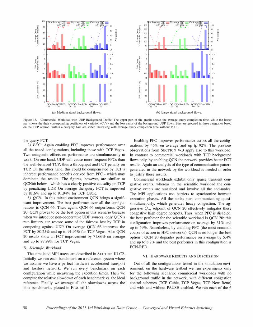
The results for the average flow completion time for the

TCP queries are shown in FIGURE 13 together with their

corresponding coefficient of variation values. In addition, in

the lower part of the figure we represent the loss ratio for

the UDP flows – the ratio is computed as the percentage

of dropped bytes vs. the total amount of injected bytes. We

observe that most of the dropped bytes are originating in UDP

flows. We consider that this is due to the lack of any congestion

control mechanism in the UDP protocol. Indeed, TCP is able

to reduce its congestion window and reduce its transmission

rate whenever losses are detected in the network.

1) TCP Vegas, TCP New Reno, TCP Cubic: In contrast with

the previous section, in this scenario all the TCP versions are

sensitive to ECN-RED and QCN, including TCP Vegas. This

can be due to the effect of the UDP being throttled strongly by

ECN or QCN, thereby leaving more network capacity available

for the TCP flows. In addition, the CoV for the query FCT

has high values up 2.8 for TCP Cubic. This shows unstable

network conditions and it reduces the confidence interval for

Proceedings of the 2011 3rd Workshop on Data Center — Converged and Virtual Ethernet Switching 57

0

20

40

60

80

QCN66

Base QCN20

RED QCN20

QCN66

Base RED QCN66

Base QCN20

RED 0

20

40

60

UD

P L

oss

Rat

io [

%]

0

0.5

1

1.5

2

2.5

0

0.5

1

1.5

2

2.5

CoV

Que

ryC

ompl

etio

n T

ime

0

20

40

60

80

100

-20

0

20

40

60

80

Ave

rage

Que

ryC

ompl

etio

n T

ime

[ms]

PFC

gai

n [%

]

New Reno w/o PFCw/ PFC

PFC gain

Vegas w/o PFCw/ PFC

PFC gain

Cubic w/o PFCw/ PFC

PFC gain

(a) Medium sized background flows.

0

20

40

60

80

QCN66

QCN20

Base RED QCN20

QCN66

Base RED QCN66

QCN20

Base RED 0

20

40

60

UD

P L

oss

Rat

io [

%]

0

0.5

1

1.5

2

2.5

0

0.5

1

1.5

2

2.5

CoV

Que

ryC

ompl

etio

n T

ime

0

50

100

150

200

250

300

-20

0

20

40

60

80

100

Ave

rage

Que

ryC

ompl

etio

n T

ime

[ms]

PFC

gai

n [%

]

New Reno w/o PFCw/ PFC

PFC gain

Vegas w/o PFCw/ PFC

PFC gain

Cubic w/o PFCw/ PFC

PFC gain

(b) Large sized background flows.

Figure 13. Commercial Workload with UDP Background Traffic. The upper part of the graphs shows the average query completion time, while the lowerpart shows the their corresponding coefficient of variation (CoV) and the loss ratios of the background UDP flows. Bars are grouped in three categories basedon the TCP version. Within a category bars are sorted increasing with average query completion time without PFC.

the query FCT.2) PFC: Again enabling PFC improves performance over

all the tested configurations, including those with TCP Vegas.

Two antagonist effects on performance are simultaneously at

work. On one hand, UDP will cause more frequent PFCs than

the well-behaved TCP; thus a throughput and FCT penalty on

TCP. On the other hand, this could be compensated by TCP’s

inherent performance benefits derived from PFC - which may

dominate the results. The figures, however, are similar to

QCN66 below - which has a clearly positive causality on TCP

by penalizing UDP. On average the query FCT is improved

by 81.6% and up to 91.94% for TCP Cubic.3) QCN: In this mixed environment QCN brings a signif-

icant improvement. The best performer over all the configu-

rations is QCN 66. Thus, again, QCN 66 outperforms QCN

20. QCN proves to be the best option in this scenario because

when we introduce non-cooperative UDP sources, only QCN’s

rate limiters can restore some of the fairness lost by TCP in

competing against UDP. On average QCN 66 improves the

FCT by 80.25% and up to 91.95% for TCP Vegas. Also QCN

20 results show an FCT improvement by 71.66% on average

and up to 97.99% for TCP Vegas.

D. Scientific Workload

The simulated MPI traces are described in SECTION III-C2.

Initially we run each benchmark on a reference system where

we assume we have a perfect hardware accelerated transport

and lossless network. We run every benchmark on each

configuration while measuring the execution times. Then we

compute the relative slowdown of each benchmark vs. the ideal

reference. Finally we average all the slowdowns across the

nine benchmarks, plotted in FIGURE 14.

Enabling PFC improves performance across all the config-

urations by 45% on average and up tp 92%. The previous

observations from SECTION V-B apply also to this workload.

In contrast to commercial workloads with TCP background

flows only, by enabling QCN the network provides better FCT

results. Again an analysis of the type of communication pattern

generated in the network by the workload is needed in order

to justify these results.

Commercial workloads exhibit only sparse transient con-

gestive events, whereas in the scientific workload the con-

gestive events are sustained and involve all the end-nodes.

The MPI applications use barriers to synchronize between

execution phases. All the nodes start communicating quasi-

simultaneously, which generates heavy congestion. The ag-

gressive Qeq setpoint of QCN 20 effectively mitigates these

congestive high degree hotspots. Thus, when PFC is disabled,

the best perfomer for the scientific workload is QCN 20: this

configuration improves performance on average by 31% and

up to 59%. Nonetheless, by enabling PFC (the most common

course of action in HPC networks), QCN is no longer the best

option : QCN 20 degrades performance on average by 5.4%

and up to 8.2% and the best performer in this configuration is

ECN-RED.

VI. HARDWARE RESULTS AND DISCUSSION

Out of all the configurations tested in the simulation envi-

ronment, on the hardware testbed we run experiments only

for the following scenario: commercial workloads with no

background traffic in the network, with different congestion

control schemes (TCP Cubic, TCP Vegas, TCP New Reno)

and with and without PAUSE enabled. We run each of the 6

58 Proceedings of the 2011 3rd Workshop on Data Center — Converged and Virtual Ethernet Switching

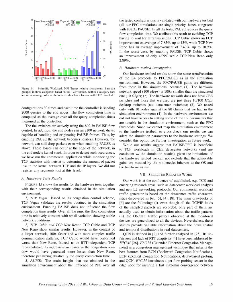
0

5

10

15

20

25

30

35

QCN66

QCN20

Base RED RED QCN20

Base QCN66

QCN20

QCN66

Base RED-20

0

20

40

60

80

100Sl

owdo

wn

Fact

or

PFC

gai

n [%

]

New Reno w/o PFCw/ PFC

PFC gain

Vegas w/o PFCw/ PFC

PFC gain

Cubic w/o PFCw/ PFC

PFC gain

Figure 14. Scientific Workload: MPI Traces relative slowdowns. Bars aregrouped in three categories based on the TCP version. Within a category barsare in increasing order of the relative slowdown factors with PFC disabled.

configurations 30 times and each time the controller is sending

2000 queries to the end nodes. The flow completion time is

computed as the average over all the query completion times

measured at the controller.

The the switches are actively using the 802.3x PAUSE flow

control. In addition, the end nodes run an e100 network driver

capable of handling and originating PAUSE frames. Thus, by

enabling PAUSE the network becomes lossless. However, the

network can still drop packets even when enabling PAUSE as

above. These losses can occur at the edge of the network, in

the end node’s kernel stack. In order to detect such occurences,

we have run the commercial application while monitoring the

TCP statistics with netstat to determine the amount of packet

loss in the kernel between TCP and the IP layers. We did not

register any segments lost at this level.

A. Hardware Tests Results

FIGURE 15 shows the results for the hardware tests together

with their corresponding results obtained in the simulation

environment.

1) TCP Vegas: Based on its congestion control scheme,

TCP Vegas validates the results obtained in the simulation

environment. Enabling PAUSE does not influence the flow

completion time results. Over all the runs, the flow completion

time is relatively constant with small variation showing stable

network conditions.

2) TCP Cubic and TCP New Reno: TCP Cubic and TCP

New Reno show similar results. However, in the context of

a larger network, 100x faster and with more complex traffic

communication patterns, TCP Cubic would have performed

worse than New Reno. Indeed, as an RTT-independent TCP

representative, its aggressive increases in the congestion win-

dow would have generated more losses than New Reno,

therefore penalizing drastically the query completion time.

3) PAUSE: The main insight that we obtained in the

simulaton environment about the influence of PFC over all

the tested configurarions is validated with our hardware testbed

(all our PFC simulations are single priority, hence congruent

with 802.3x PAUSE). In all the tests, PAUSE reduces the query

flow completion time. We attribute this result to avoiding TCP

having to wait for retransmissions. TCP Cubic shows an FCT

improvement on average of 7.85%, up to 13%, while TCP New

Reno has an average improvement of 7.43%, up to 10.9%.

In the worst case, by enabling PAUSE, TCP Cubic shows

an improvement of only 4.09% while TCP New Reno only

2.89%.

B. Hardware testbed investigation

Our hardware testbed results show the same trend/reaction

of the L4 protocols to PFC/PAUSE as in the simulation

environment. However, the PFC/PAUSE gains are different

from those in the simulations, because: (1). The hardware

network speed (100 Mbps) is 100x smaller than the simulated

one (10 Gbps); (2). The hardware network does not have CEE

switches and those that we used are just three 10/100 Mbps

desktop switches (not datacenter switches); (3). We tested

only with 10 nodes against the 80 clients that we had in the

simulation environment; (4). In the hardware environment we

did not have access to setting some of the L2 parameters that

are tunable in the simulation environment, such as the PFC

thresholds. Since we cannot map the simulation environment

to the hardware testbed, to cross-check our results we can

adapt the simulation parameters to the hardware settings. We

consider this option for further investigation as future work.

While our results suggest that PAUSE/PFC is beneficial

to TCP workloads in CEE datacenter networks (and are

consistent w/ the simulation results), given the limitations of

the hardware testbed we can not exclude that the achievable

gains are masked by the bottlenecks inherent to the OS and

the hardware in use.

VII. SELECTED RELATED WORK

Our work is at the confluence of established, e.g. TCP, and

emerging research areas, such as datacenter workload analysis

and new L2 networking protocols. Our commercial workload

traffic generator is based on the datacenter traffic character-

istics discovered in [6], [5], [4], [8]. The main drawbacks of

[6] are the following: (i). even though all the TCP/IP fields

of the sampled packets are recorded, only part of them are

actually used to obtain information about the traffic pattern;

(ii). the ON/OFF traffic pattern observed at the monitored

devices are generalized to all the devices. Nevertheless, these

studies provide valuable information about the flows spatial

and temporal distributions in real datacenters.

QCN is defined in [2] and further analyzed in [25]. Its un-

fairness and lack of RTT adaptivity [4] have been addressed by

E2CM [26]. E2CM (Extended Ethernet Congestion Manage-

ment) is a congestion management technique that inherits the

best features from BCN (Backward Congestion Notification),

ECN (Explicit Congestion Notification), delay-based probing

and QCN. E2CM introduces a per-flow probing sensor in the

edge node for insuring a fast max-min convergence between

Proceedings of the 2011 3rd Workshop on Data Center — Converged and Virtual Ethernet Switching 59

0

200

400

600

New Reno Vegas Cubic-5

0

5

10

15A

vera

ge Q

uery

Com

plet

ion

Tim

e [m

s]

PFC

gai

n [%

]

w/o PFCw/ PFC

PFC gain

w/o PFCw/ PFC

PFC gain

w/o PFCw/ PFC

PFC gain

(a) Hardware Testbed Results.

0

1

2

3

4

New Reno Vegas Cubic-5

5

15

25

35

45

55

Ave

rage

Que

ryC

ompl

etio

n T

ime

[ms]

PFC

gai

n [%

]

w/o PFCw/ PFC

PFC gain

w/o PFCw/ PFC

PFC gain

w/o PFCw/ PFC

PFC gain

(b) Simulation Results.

Figure 15. Hardware vs. Simulation Results: (a) shows the query completion times obtained in the hardware environment, their corresponding 95% confidenceintervals and the PFC gains (the three black dots); (b) shows the query completion times obtained in the simulation environment and their corresponding PFCgains (the three black dots).

the flows, even without fair share and rate-based computations

in the bridge. This scheme manages to eliminate the drawbacks

of BCN (slow convergence, unfairness and oscillations) and

increases convergence and scalability with network size. An

alternative solution is AF-QCN, proposed in [27]. AF-QCN

keeps the QCN simplicity, responsiveness and stability features

and improves the QCN fairness by providing a programmable

bandwidth partitioning per-flow or per-class of traffic.

The TCP Incast problem has been analyzed in [7], [10],

[4]. TCP Incast happens in the context of barrier synchro-

nized many-to-one traffic in high bandwidth and low latency

networks like datacenter networks. This type of traffic, as in

scatter/gather, generates traffic with a high degree of bursti-

ness. Even if it is temporarily, bursty traffic can cause packet

loss and retransmissions which would increase the application

response time. One solution is suggested in [10] where a

10 − 1000× RTO reduction and high resolution timers have

been proposed. Another TCP Incast solution is DCTCP [4],

using a modified RED/ECN, a new multibit feedback estimator

that filters the incoming single-bit ECN stream and a modified

TCP at both sender and receiver sides. By contrast, [7] brings

a solution based on TCP changes at the receiver side only.

Closely related is [24] which analyzes the TCP Incast problem

in a QCN-enabled lossy network – arguably in conflict with

default assumption of lossless CEE. The authors propose a

new version of QCN with adaptive sampling at the congestion

point and adaptive rate increase at the reaction point. The main

drawbacks are the use of NS-2 simulations and the overly

aggressive sampling proposal.

Finally, most recent and relevant for the experimental

part of our assessment, TCP Incast is studied in [9] using

SCTP and ECN with hardware experiments. The performance

improvements range from 5.5% to 7.9%, most likely lim-

ited by the experimental platform. Although unrelated and

complementary to our experimental hardware and software

platform, the notably similar performance improvement ranges

between these two independent studies prompt for further in-

vestigation. While experimental results in the field traditionally

constitute the ultimate validation, the recent improvements in

performance, accuracy and capacity make simulations a key

modeling tool for datacenter research.

VIII. CONCLUSIONS AND FINAL REMARKS

In this paper we have performed an extended evaluation

of the TCP performance over CEE datacenter networks as

initially introduced in [28]: The main difference here is in

employing two modeling methods, i.e., the Omnet++ Venus

ZRL simulation platform, and, an adhoc hardware testbed. In

simulation, we used as traffic generators three types of work-

loads: congestive synthetic traffic, commercial and scientific

applications. In hardware, we emulated and tested commercial

workloads only. The hardware testbed – albeit reduced in

speed and scale – still validates the main results obtained from

simulations. We summarize the results obtained by answering

the original questions from SECTION I.

(Q1) How does TCP perform over CEE networks?: In both

simulation and hardware environments, the delay-probing TCP

Vegas remains the best performer as before in [28], requiring

the same minimal changes, e.g., high resolution timers. By

contrast, as an RTT-independent TCP representative, Cubic

entails the most adaptation effort for datacenter environments,

eliciting parameter tuning and potentially core algorithmic

changes - which we have not performed. Indeed, because of

its aggressivity and slow convergence of congestion windows,

Cubic as it stands today does not seem the most suitable

transport protocol for datacenter networks. Even though it

was only partly CEE-enabled, also the hardware enviroment

confirms that Cubic yields worse FCT results. Whether the

RTT independence, as in BIC and Cubic, is harmful in CEE

networks with high variations of queueing delays, from 0.5

μs up to tens of ms, remains an open problem. TCP New

Reno lies in between the two extremes above, requiring more

parametrical retuning than Vegas, but no invasive changes such

as Cubic - while producing promising performance results.

60 Proceedings of the 2011 3rd Workshop on Data Center — Converged and Virtual Ethernet Switching

New Reno’s key features as a DCN transport candidate are in

its relative simplicity of operation, ubuiquity and compatibility

with AQM methods such as RED and REM. We argue that

TCP Vegas currently is our best transport protocol candidate

for CEE datacenter networks. To achieve its full performance

potential some changes are suggested.

1) Increased time granularity: a finer granularity allows for

(much) more precise RTT measurements. To obtain a

finer time granularity in Linux, one can increase the

HZ kernel parameter - directly changing the ’jiffy’ time

reference of the TCP code. A more complex method

would be to modify the TCP kernel code to implement a

finer time reference for the time sensitive modules. Time

sources with finer granularity than jiffies do exist, e.g..

Linux doGetTimeOfDay directly queries the hardware

and it is not updated when the timer ticks – though they

are complex and architecture-dependent, possibly elic-

iting an increased CPU overhead. A trade-off between

TCP performance and CPU overhead study is left as an

interesting future work.

2) Default RTO: The current Linux kernels have a de-

fault initial RTO value of 3s. If the first TCP SYN

packet is lost, the source will have to wait 3s before

retransmitting the packet and re-initiating the connec-

tion. This affects drastically the flow completion time

in a DCN environment and, the performance of delay

sensitive applications such as, business analytics, algo-

rithmic trading and P/A workloads. The problem can

be mitigated by setting the default initial RTO to a

small multiplier of the maximum RTT of the datacenter

network when fully congested. The multiplier should be

conservative enough, since a smaller RTO (then RTTmax)

can trigger false positives: unnecessary retransmissions,

thus wasting bandwidth and again degrading the network

performance.

(Q2) Is PFC beneficial or detrimental to TCP?: Despite

our initially different expectations, PFC has systematically

improved performance across all the tested configurations

and benchmarks in both the simulation and the hardware

environments. In simulation, the commercial workload com-

pletion time improves by 27% on average, and up to 91%.

Scientific workloads show higher gains by enabling PFC:

45% on average, and up to 92%. In hardware, over all the

configurations, the results show the same positive trend by

enabling PFC (our case, single priority PAUSE). On average,

PFC increases performance by 6.45% and up to 13%. Note

on PFC tuning: PFC implementation in input buffer and dis-

tributed crossbar switches is relatively straightforward, except

the optimal settings of the two thresholds.

The upper limit (STOP) should be set as high as possible,

but low enough to ensure that once it is reached and the

PFC=ON frame is sent out, the buffer has enough remaining

space to accomodate all the still in-flight packets that the

upstream source might have sent before receiving the noti-

fication. The amount of in-flight traffic can be calculated as

maximum between the local link level RTT plus the logical

delays times the maximum injection rate (BDP), and, the

worst-case MTU, i.e. 2x the largest MTU supported (2 Jumbo

frames). This value may or not coincide with the PFC timing

recommendations made by 802 DCB in bit time units.

The lower limit (GO) must be set to (i) avoid oscillations

(PFC=ON/OFF/ON...) through a sufficiently wide hysteresis,

(ii) reduce the ’dead time’ to restart (prevent underflow),

and, (iii) prevent the synchronized restarts of multiple traffic

sources.

The PFC gains recorded from our hardware testbed are no-

tably inferior to those obtained in the simulation. We attribute

this discrepancy to the practical limitations of our testbed: the

consumer-level hardware is not CEE equipped, works at 100xslower rate than the 10 Gbps simulation platform, and the

hardware ’datacenter’ network contains 5x less end nodes .

We plan to redo the experiments in a more realistic datacenter

testbed, with direct access to the hardware CEE configuration

of the network. Currently we are not aware of the availability

of DCN switches and adapters implementing user-accessible

CEE and OpenFlow interfaces, as required to conduct our

investigation.

(Q3). Is QCN beneficial or detrimental to TCP?: The answer

to this question must be more carefully qualified, depending

on (a) whether TCP is alone, or in competition with (e.g.)

UDP traffic; (b) the proper parameter settings per type of

application. Given the available hardware capabilities, we

tested the TCP performance over QCN only in the simulation

environment.

On the positive side, properly tuned for mixed environments

of commercial TCP with UDP applications, QCN 66 with

PFC improves performance on average by 49%, up to 70%.

Regardless of the upper layer protocols, QCN 66 succeds to

keep congestion under control even when we introduce in the

network non-cooperative, greedy UDP flows. For scientific

workloads QCN 20 without PFC improves performance on

average by 31%, up to 59%. HPC applications typically exhibit

alternating phases of computation and communication. During

the latter, typically all nodes start communicating almost at the

same time, which can generate heavy congestion, especially in

slim networks as simulated here. The aggressive Qeq setpoint

of QCN 20 effectively mitigates such congestive events.

On the negative side, mistuned QCN can severely degrade

performance. For example, for the commercial workload with-

out UDP, QCN 20 without PFC degrades performance on

average 131%, up to 311% for New Reno and 321% for

Cubic. For scientific workloads QCN 66 with PFC degrades

performance on average by 5.4%, up to 8.2%. QCN suffers

also from inherent unfairness as it tends to randomly favor

only some of the flows over the others harming the average

completion time.

As a conclusion for Q3, we argue that QCN needs further

investigation and improvement with respect to adaptivity and

fairness. Even if QCN is customizable also by the means of

the Qeq parameter, setting its value is more challenging than

that of the PFC thresholds. As one example, is improvement of

Proceedings of the 2011 3rd Workshop on Data Center — Converged and Virtual Ethernet Switching 61

QCN’s burst tolerance: Can be trivially achieved by increasing

the setpoint values, such as Qeq = 66 (much higher than the

.1Qau recommendation). Another –albeit complex and non-

standard– option to improve the QCN burst tolerance would be

to set a low Qeq= [8-17], and to filter the (multibit) congestion

feedback notifications stream at the source, somewhat similar

to single-bit DCTCP feedback in [4]. When in doubt about

the nature of their DC workloads and QCN’s impact on the

performance, the datacenter managers may consider QCN for

conservative deployment: Hence, originally the equillibrium

point should be set starting from high values (Qeq = 80 or

Qeq = 90) that will minimize the amount of false positivies

and the QCN activity (relax its control loop). Subsequently,

the QCN loop can be progressively tightened by reducing

Qeqtoward the .1Qau recommended values. It is essential

that this manual QCN tuning is performed while carefully

monitoring the DCN performance.Finally we have also shown results of TCP with RED. Our

simulation results show that RED can handle the transient con-

gestion episodes generated by commercial applications better

than QCN. Properly configured, RED is less sensitive to bursty

traffic than QCN. Indeed, RED relies on smoothed queue

length and not on instantaneous queue size as QCN does. By

contrast, QCN has an intrinsic higher burst-sensitivity than

RED. However, this can be prevented by properly configuring

its setpoint Qeq . The simulation results showed that RED

can reduce the query completion time by up to 76%, which

suggests that future CEE switches should implement RED, and

other such L3 primitives directly in L2.Future Work: We intend to cross-validate the results ob-

tained for the hardware setup through an accurate simulation

of the actual platform used. Foremost, our experimental testbed

must be upgraded with new CEE-compatible switches and

adapters. Currently this is our main limitation. We aim to

build a CEE virtualized network environment (already partially

instrumented) and test it under the same workloads and

configurations.

ACKNOWLEDGMENTS

We are deeply indebted to C. Minkenberg for his contribu-

tions.

REFERENCES

[1] P802.1Qbb/D1.3 Virtual Bridged Local Area Networks - Amendment:

Priority-based Flow Control, IEEE Draft Standard, 2010. [Online].Available: http://www.ieee802.org/1/pages/802.1bb.html

[2] P802.1Qau/D2.4 Virtual Bridged Local Area Networks - Amendment:

Congestion Notification, IEEE Draft Standard, 2009. [Online]. Available:http://www.ieee802.org/1/pages/802.1au.html

[3] M. Gusat et al., “Delay-based Cloud Congestion Control,” in Proc. IEEE

GLOBECOM 2009 Global Communications Conference, Honolulu, HI,USA, December 2009.

[4] M. Alizadeh et al., “DCTCP: Efficient Packet Transport for the Com-moditized Data Center,” in Proc. ACM SIGCOMM 2010 Conference on

Data Communication, New Delhi, India, August 2010.[5] T. Benson et al., “Network Traffic Characteristics of Data Centers

in the Wild,” in Proc. Internet Measurement Conference (IMC 2010),Melbourne, Australia, November 2010.

[6] ——, “Understanding Data Center Traffic Characteristics,” in Proc.

ACM SIGCOMM Workshop for Research on Enterprise Networks

(WREN 2009), Barcelona, Spain, August 2009.

[7] Y. Chen et al., “Understanding TCP Incast Throughput Collapse inDatacenter Networks,” in Proc. 1st ACM Workshop on Research on

Enterprise Networking (WREN 2009), Barcelona, Spain, August 2009.[8] S. Kandula et al., “The Nature of Datacenter Traffic: Measurements

& Analysis,” in Proc. Internet Measurement Conference (IMC 2009),Chicago, IL, USA, November 2009.

[9] R. R. Stewart et al., “An Investigation into Data Center Congestionwith ECN,” in Proc. 2011 Technical BSD Conference (BSDCan 2011),Ottawa, Canada, May 2011.

[10] V. Vasudevan et al., “Safe and Effective Fine-grained TCP Retransmis-sions for Datacenter Communication,” in Proc. ACM SIGCOMM 2009

Conference on Data Communication, Barcelona, Spain, August 2009.[11] J. Dean and S. Ghemawat, “MapReduce: Simplified Data Processing on

Large Clusters,” in Proc. 6th Symposium on Operating System Design

and Implementation (OSDI 2004), San Francisco, CA, USA, December2004.

[12] S. R. Öhring et al., “On Generalized Fat Trees,” in Proc. 9th Interna-

tional Parallel Processing Symposium (IPPS 1995), Santa Barbara, CA,USA, April 1995.

[13] S. Floyd and V. Jacobson, “Random Early Detection Gateways forCongestion Avoidance,” IEEE/ACM Transactions on Networking, vol. 1,no. 4, pp. 397–413, August 1993.

[14] RFC 3782, RFC, April 2004. [Online]. Available:http://www.faqs.org/rfcs/rfc3782.html

[15] I. Rhee and L. Xu, “CUBIC: A New TCP-Friendly High-Speed TCPVariant,” in Proc. PFLDnet, Lyon, France, February 2005.

[16] L. Brakmo et al., “TCP Vegas: New Techniques for Congestion De-tection and Avoidance,” in Proc. ACM SIGCOMM 1994 Conference on

Data Communication, London, UK, August 1994.[17] C. Minkenberg and G. Rodriguez, “Trace-driven Co-simulation of High-

Performance Computing Systems using OMNeT++,” in Proc. SIMU-

Tools 2nd International Workshop on OMNeT++, Rome, Italy, March2009.

[18] G. Rodriguez, “Understanding and Reducing Contention in GeneralizedFat Tree Networks for High Performance Computing,” Ph.D. disserta-tion, Technical University of Catalonia, Barcelona, Spain, 2011.

[19] RFC 2988 - Computing TCP’s Retransmission Timer, RFC, November2000. [Online]. Available: http://potaroo.net/ietf/idref/rfc2988/

[20] K. Tan and J. Song, “A compound tcp approach for high-speed and longdistance networks,” in In Proc. IEEE INFOCOM, 2006.

[21] N. Dukkipati and N. McKeown, “Why Flow-Completion Time is theRight Metric for Congestion Control,” ACM SIGCOMM Computer

Communication Review, vol. 36, no. 1, pp. 59–62, January 2006.[22] D. Bailey et al., “The NAS Parallel Benchmarks,” NASA Ames Research

Center, Moffett Field, CA, NASA Technical Report RNR-94-007, March1994.

[23] Y. Etsion et al., “Effects of Clock Resolution on the Scheduling of Real-Time and Interactive Processes,” in SIGMETRICS ’03 Proceedings of the

2003 ACM SIGMETRICS international conference on Measurement and

modeling of computer systems.[24] P. Devkota and A. L. N. Reddy, “Performance of Quantized Congestion

Notification in TCP Incast Scenarios of Data Centers,” in Proc. 2010

IEEE International Symposium on Modeling, Analysis and Simulation

of Computer and Telecommunication Systems (MASCOTS 2010), MiamiBeach, FL, USA, August 2010.

[25] C. Minkenberg and M. Gusat, “Congestion Management for 10G Eth-ernet,” in Proc. Second Workshop on Interconnection Network Archi-

tectures: On-Chip, Multi-Chip (INA-OCMC 2008), Goteborg, Sweden,January 2008.

[26] M. Gusat et al. (2007, March) Extended Ethernet CongestionManagement (E2CM): Per Path ECM - A Hybrid Proposal. [Online].Available: http://ieee802.org/1/files/public/docs2007/au-sim-IBM-ZRL-E2CM-proposal-r1.09.pdf

[27] A. Kabbani et al., “AF-QCN: Approximate Fairness with QuantizedCongestion Notification for Multi-tenanted Data Centers,” in Proc. 18th

Annual IEEE Symposium on High-Performance Interconnects (HOTI

2010), Mountain View, CA, USA, August 2010.[28] D. Crisan et al., “Short and Fat: TCP Performance in CEE Datacenter

Networks,” in HOT Interconnects (HOTI 2011), Santa Barbara, Califor-nia, US, August 2011.

62 Proceedings of the 2011 3rd Workshop on Data Center — Converged and Virtual Ethernet Switching