crowd space: a predictive crowd analysis techniqueioannis/crowd-space/files/crowdspa… · crowd...

Crowd Space: A Predictive Crowd Analysis Technique

IOANNIS KARAMOUZAS, Clemson UniversityNICK SOHRE, University of MinnesotaRAN HU, Facebook & University of MinnesotaSTEPHEN J. GUY, University of Minnesota

Over the last two decades there has been a proliferation of methods forsimulating crowds of humans. As the number of different methods andtheir complexity increases, it becomes increasingly unrealistic to expectresearchers and users to keep up with all the possible options and trade-offs.We therefore see the need for tools that can facilitate both domain expertsand non-expert users of crowd simulation in making high-level decisionsabout the best simulation methods to use in different scenarios. In this paper,we leverage trajectory data from human crowds and machine learning tech-niques to learn a manifold which captures representative local navigationscenarios that humans encounter in real life. We show the applicability ofthis manifold in crowd research, including analyzing trends in simulation ac-curacy, and creating automated systems to assist in choosing an appropriatesimulation method for a given scenario.

CCS Concepts: • Computing methodologies → Animation; Multi-agentplanning; Scene understanding; •Mathematics of computing→ Dimen-sionality reduction;

Additional Key Words and Phrases: Crowd simulation, validation, entropy,manifold learning

ACM Reference Format:Ioannis Karamouzas, Nick Sohre, Ran Hu, and Stephen J. Guy. 2018. CrowdSpace: A Predictive Crowd Analysis Technique. ACM Trans. Graph. 37, 6, Ar-ticle 186 (November 2018), 14 pages. https://doi.org/10.1145/3272127.3275079

1 INTRODUCTIONThe last two decades have seen a dramatic rise in the number oftechniques used in simulating real-world phenomena, from animat-ing fluid and sound to modeling hyperelastic materials and humancrowds [Bridson 2015; Lee 2010; Pelechano et al. 2016; Sifakis andBarbic 2012]. In many fields, this growth in choice of simulationmethods raises many questions for domain experts in choosing ap-propriate simulation techniques. This is especially true in the fieldof human crowd simulation, where there are a large number of sim-ulation methods that all preform well in some scenarios, but noneof which performs “best" in all scenarios. However, choosing theright simulation method can be very important. When crowds areused in games and movies, poor simulation performance can lead to

Authors’ addresses: Ioannis Karamouzas, Clemson University, [email protected];Nick Sohre, University of Minnesota, [email protected]; Ran Hu, Facebook & Univer-sity of Minnesota, [email protected]; Stephen J. Guy, University of Minnesota,[email protected].

Permission to make digital or hard copies of all or part of this work for personal orclassroom use is granted without fee provided that copies are not made or distributedfor profit or commercial advantage and that copies bear this notice and the full citationon the first page. Copyrights for components of this work owned by others than theauthor(s) must be honored. Abstracting with credit is permitted. To copy otherwise, orrepublish, to post on servers or to redistribute to lists, requires prior specific permissionand/or a fee. Request permissions from [email protected].© 2018 Copyright held by the owner/author(s). Publication rights licensed to Associationfor Computing Machinery.0730-0301/2018/11-ART186 $15.00https://doi.org/10.1145/3272127.3275079

unnatural crowd behavior, quickly breaking the immersion. Whencrowd simulations are used to guide event planning and buildingdesign, poor simulation models can lead to bad practices affectingthousands of people.Domain experts in crowd simulations, as in many fields, have a

wealth of informal knowledge about what simulation approachesto use when. Many experts will suggest not to use reactive methodssuch as social forces or boids [Helbing et al. 2000; Reynolds 1987]unless the simulation task involves a small number of agents insparse scenarios. Likewise, many researchers tend to feel geometricmethods such as ORCA [van den Berg et al. 2011] are likely tostruggle in medium density scenarios where agile maneuvers areimportant, but do well in dense scenarios where efficient accountingfor constraints is key. This kind of informal, unquantified knowledgeis crucial to the proper choice of simulation method, but cannotalways be reliably communicated in an objective and universallyaccesible fashion.In this paper, we propose to leverage data-driven learning tech-

niques to develop a method to compactly represent this type ofmeta-information about crowd simulation scenarios. To this end,we introduce Crowd Space, a low-dimensional manifold learned fromhuman trajectories, which represents the space of likely interactionscenarios that humans can encounter (see Figure 1). We also learn acontinuous labeling of this manifold based on a novel method thatallows us to evaluate the local simulation accuracy.

Ultimately, our work provides a method for formalizing and quan-tifying knowledge about what types of simulation techniques touse in different scenarios. To that end, we propose the followingcontributions:

• Crowd Space. An agent-centric, low-dimensional manifoldrepresenting a large variety of crowd interaction scenarios.

• An agent-centric formulation of the entropy metric of [Guyet al. 2012] that allows the estimation of a simulation’s localaccuracy.

• An analysis of key trade-offs between simulation methods,alongwith a learning-based approach to automatically predictthe best (i.e., most accurate) simulation methods to use in agiven scenario.

2 RELATED WORK

2.1 Multi-Agent Navigation MethodsThere is a significant amount of research in robotics, traffic engineer-ing, and computer graphics on planning paths for multiple agentssuch as virtual characters, pedestrians, and cars. The most com-mon approach is to decompose global planning from local collisionavoidance. Typically, a graph is used to capture paths which arecollision-free with respect to the static part of the environment,

ACM Transactions on Graphics, Vol. 37, No. 6, Article 186. Publication date: November 2018.

https://doi.org/10.1145/3272127.3275079

https://doi.org/10.1145/3272127.3275079

186:2 • Ioannis Karamouzas, Nick Sohre, Ran Hu, and Stephen J. Guy

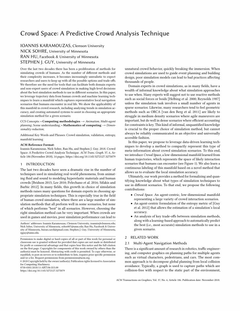
Fig. 1. Crowd space embedding using PCA. The space is obtained by sampling 15,000 60D mpd-based local scenario descriptors gathered from six trainingdatasets (2,500 descriptors per dataset), and taking the first 6 principal components. Here, we visualize this 6D space by random sampling of non-overlappingdescriptors and plotting them according to their first two principle components. The resulting space clusters together agents with similar local conditions,even if they come from different datasets. In this 2D projection, the horizontal axis tends to correspond to density (more dense on the left) and the vertical axiswhether the agent is entering, leaving, or located in the middle of congestion (top, bottom, middle, respectively). The edges in the 2D embedding denotenearest neighbors.

and a local collision avoidance technique is then used to navigateeach agent around other nearby agents and obstacles. Our workhere will focus on the local navigation, as many different methodsrely on the same global planning approaches (e.g., artist-designedroadmaps), and variation in global planning tend to have less in-fluence on the collective behavior of the agents than variation inlocal planning. (We refer the reader to the recent books of [Kapadiaet al. 2015; Pelechano et al. 2016] for a more extensive review ofstate-of-the-art local navigation and global planning approaches.)While a large variety of local navigation methods have been

proposed, many popular methods can be classified into one offive classes: a) reactive approaches where agents rely primarily ondistance-based functions to avoid collisions with nearby agents andobstacles [Helbing et al. 2000; Helbing and Molnár 1995; Reynolds1999]; b) geometrically-based approaches where agents computecollision-free velocities using sampling or optimization [Pettré et al.2009; van den Berg et al. 2011, 2008], c) vision-based approacheswhere the steering behavior of each agent is directly correlatedto its (simulated) visual stimuli [Hughes et al. 2015; Kapadia et al.2012; Moussaïd et al. 2011; Ondřej et al. 2010]; d) gradient-basedapproaches where each agent tries to independently minimize anenergy or cost function that accounts for future collisions [Dutraet al. 2017; Karamouzas et al. 2014; Wolinski et al. 2016]; and e)example-based approaches that use human data to update the veloc-ities of simulated agents [Charalambous and Chrysanthou 2014; Juet al. 2010; Lerner et al. 2007]. Here, we do not consider example-based approaches directly, as their accuracy depends directly onhow closely their training dataset matches our testing dataset, ratherthan how well their mathematical models capture human behavior.There are, of course, navigation methods that do not fit easily

into one of these categories. For example, some methods focus onexplicitly accounting for grouping and other social dynamics [Ren

et al. 2017], level-of-detail methods [Kulpa et al. 2011], and meth-ods that closely model the biomechanics of body orientation andfootstep patterns [Singh et al. 2011; Stuvel et al. 2016]. Furthermore,with recent advancements in deep learning, approaches have beenintroduced that seek to improve the collision avoidance behaviorand the locomotion of the agents [Holden et al. 2017; Long et al.2017; Peng et al. 2017].

2.2 Data-driven evaluation and analysisPerhaps the most intuitive way to analyze the accuracy of a sim-ulated crowd is by defining a number of test-case scenarios alongwith evaluation metrics that can be used to collect statistics aboutthe behavior of the agents. For example, Reitsma and Pollard [2007]used task-based metrics to evaluate the animation capabilities ofvirtual agents, while the work in [Kapadia et al. 2009, 2011; Singhet al. 2009] focus on the steering behavior of the agents. Such met-rics have also been used by data-driven evaluation techniques todetermine how similar are simulated pedestrians to real ones ex-tracted from video crowd footage [Lerner et al. 2010]. This includeapproaches that automatically detect outlying behavior [Charalam-bous et al. 2014] and optimization-based techniques that tune theparameters of the agents to enable simulations that best fit the givendata [Berseth et al. 2014; Wolinski et al. 2014]. Evaluation techniquesthat focus on the macroscopic behavior of the agents have also beenproposed, such as the work in [Wang et al. 2017] that uses Bayesianinference to learn path patterns and compare them to referencedata, and the entropy metric work [Guy et al. 2012] that estimatesin a robust way the similarity between the aggregate motion of realpedestrian and simulated trajectories.

Our work is complementary to the crowd evaluation techniquesmentioned above. In particular, we extend the entropy work to


Crowd Space: A Predictive Crowd Analysis Technique • 186:3

focus on the predictive accuracy of a simulation method at a per-agent level. Furthermore, as compared to previous solutions, ourmethod learns to automatically predict the most accurate simulationmethods for a given interaction scenario. We note that there is also asignificant amount of work on perceptually evaluating simulations.In particular, user studies have been proposed in different fieldsto assess the visual quality of videos, rendering techniques, andfluid simulation methods (see, e.g., [Aydin et al. 2010; Um et al.2017]. Furthermore, perceptual studies have been extensively usedin the field of character animation and crowd simulation, with recentwork focusing on the visual realism and expressiveness of animatedcrowds [Durupinar et al. 2017; Hoyet et al. 2013; McDonnell et al.2009]. While related to our work, the goal of these approachesis somewhat orthogonal to ours, as they focus on the perceptualquality rather than the predictive accuracy of simulations.

3 BACKGROUND AND DEFINITIONSWhile the question of how to analyze different crowd simulationtechniques can take many forms, our work focuses on the follow-ing two questions: i) Given a simulation method, in what crowdscenarios does this method perform the best? And ii) Given a par-ticular crowd scenario, which methods produce the most accuratesimulations?Formally, we define the above terms as:• Crowd Scenario: A crowd simulation scenario, S, consistsof a set of n agents, each with its own initial position, goalposition, goal speed, radius, and (optionally) a set of obstaclesdemarcating impassable regions.

• Simulation Method: A simulation method is a functionwhich takes as input a crowd scenario, and returns as out-put a trajectory for each agent.

• Simulation Accuracy: The accuracy of a simulation methodis a measure of how closely the resulting trajectories matchthose which would have been produced by humans in thesame crowd scenario.

In particular, we note that there are many different plausiblemeasures of simulation accuracy (see, e.g., [Singh et al. 2009; Umet al. 2017]). Here, we focus on the notation of predictive accuracyas introduced by the Entropy Metric [Guy et al. 2012], that is: givena representative collection of real human trajectories, what is thelikelihood that a given simulation method would produce similartrajectories in similar circumstances.

3.1 Generating Scenarios from Human DataTo best estimate the accuracy of a given technique in a particularcrowd scenario, we should have access to a collection of representa-tive trajectories that real humans took in the same (or very similar)situations. While it would be best to randomly sample a well dis-tributed range of crowd scenarios and ask human subjects to enactthese situations, this approach is impractical to achieve at scale. In-stead, we invert this strategy and infer likely crowd scenarios givenpreviously observed trajectories from real-world crowd videos. Bybreaking real-world crowd datasets and videos into small time stepswe can infer hundreds of new crowd scenarios by estimating a posi-tion, velocity, radius, goal position and goal speed for each agent.

Appendix A gives details on how we estimate each of these terms.Importantly, deriving crowd scenarios from real-world data allowsus to know what paths real people took in each of these scenarios.Crowd Datasets. Because all of our crowd scenarios are derived

from real-world datasets, it it is important to choose a large, var-ied collection of human data for training. Here, we use ten dif-ferent human trajectory datasets representing efforts from a vari-ety of researchers, crowd densities, motion heterogeneity, and soon. These include: i) sparse crowds (average space-time densityless than 0.5 ppl/m2) captured at a snowy intersection [Pellegriniet al. 2009] and in front of a church [Lerner et al. 2010], labeledSnow_eth and Church, respectively; ii) Medium-density (between0.5-2 ppl/m2) groups of shoppers walking down a street at twodifferent times of day, Zara1 and Zara2, and students on a collegecampus, Students [Lerner et al. 2007]; iii) Dense groups (averagedensity greater than 2 ppl/m2) of participants in various scenariosincluding walking through differently shaped bottlenecks, labeledBottleneck and Bottleneck-long [Seyfried et al. 2009], interacting astwo large streams moving past each other through a train stationhallway, Berlin-180, and two large streams of people interactingperpendicularly Berlin-90 [Lämmel and Plaue 2014]; iv) And, finally,results from experiments with small groups walking simultaneouslydown a hallway, One-way [Ju et al. 2010].

3.2 Simulation MethodsWe investigate several different local navigation methods, repre-senting a wide variety of different simulation techniques. In gen-eral, we selected methods which are either recently proposed orin wide-spread use. This includes reactive Social Forces [Helbinget al. 2000], the geometrically-based methods of T-Model [Pettréet al. 2009] and ORCA [van den Berg et al. 2011], the Vision-basedmethod of [Moussaïd et al. 2011] which uses a sampling-based ap-proach to optimize an anticipatory energy function, and predictiveforce-based approaches of PAM [Karamouzas et al. 2009] and TTCForces [Guy and Karamouzas 2015]. Where possible, we obtainedthe latest, revised implementation directly from the authors, thoughin the case of the Social Forces and Vision-based models we providedour own implementation.

Note, we exclude the PowerLaw model proposed in [Karamouzaset al. 2014] as it was explicitly trained on part of the data used to cre-ate our learning method. Likewise, we avoid data-driven approachessuch as the ones proposed in [Charalambous and Chrysanthou 2014;Lerner et al. 2007] due to similar concerns with over-fitting. Finally,we do not consider continuum-based solutions or those which re-quire explicit global solvers such as those proposed in [Karamouzaset al. 2017; Narain et al. 2009; Treuille et al. 2006] as these methodstend to be too slow for the entropy-based accuracy analysis weemploy (Section 4) and can have difficulty with agents who enterand exit a simulation.

3.3 OrganizationThe next section details our approach to evaluating the time-varyingaccuracy with which a simulation captures the behavior of real-world pedestrians in various settings. In Section 5, we detail our



approach to building a crowd scenario manifold to facilitate sim-ulation analysis. In Section 6, we use the resulting Crowd Spaceto analyze the relative accuracy of the aforementioned simulationmethods in various scenarios. Finally, Section 7 introduces a methodto automate the process of predictive crowd analysis by formulatingit as a multi-label classification problem.

4 AGENT-CENTRIC ENTROPYIn order to facilitate our predictive analysis of various crowd simula-tion techniques, we must first establish an evaluation metric. Here,we wish to focus on the accuracy of a simulation technique; that is,how closely a simulation matches the behavior of real pedestriansin similar scenarios. Much of the previous work in this area has fo-cused on studying indirect measures of accuracy, such as comparingthe local density of simulated agents to those found in database oftypical human motion as in [Lerner et al. 2010] and [Charalambouset al. 2014], or has used user-defined metrics to evaluate a path suchas smoothness or number of collisions [Kapadia et al. 2009; Singhet al. 2009]. While these approaches are valuable metrics of pathquality, they do not directly address the predictive accuracy a simu-lation method may have in a given scenario. Closer to our goal is theentropy metric proposed in [Guy et al. 2012], which uses a stochasticinference framework to directly estimate prediction accuracy of amethod given a set of pedestrian trajectories in a manner which isrobust to the large amount of sensor noise present in real-worlddatasets. However, the original formulation of this metric has twoissues we seek to address:

(1) Fixed Simulation Size.The original entropymetric assumes thenumber of agents is static throughout a dataset. In practice,agents will likely enter and leave the scene quite frequentlyin any dataset lasting more than a few seconds.

(2) Global Accuracy Estimates. The original entropy metric pro-vides a single accuracy estimate per simulation method perdataset. In reality, the accuracy of a simulation varies spatially(per-agent), and over time (for a given agent).

In this section, we propose a per-agent entropy metric which(1) allows agents to enter and exit a scene over time and (2) pro-vides a per-agent, ego-centric estimate of how well a given crowdsimulation method would predict the motion of each agent in thecrowd. Together, these changes remove the fundamental hetero-geneity assumption found in the original entropy metric. As a result,we can now identify localized problem regions within an otherwisehigh-quality simulation method, greatly improving the metric’sapplicability for crowd analysis.

4.1 Approach OverviewSimilar to the original entropy metric approach, we seek to measurethe degree to which a simulation method is likely to produce thebehavior captured in a real-world dataset. As in [Guy et al. 2012], wefollow an information-theoretic formulation, and treat measuringaccuracy as a likelihood estimation problem. The overall approachto computing the entropy metric is as follows: first, decompose theobserved crowd data into several single time step prediction tasksby using Bayesian filtering (e.g. Kalman filtering); second, add zero-mean Gaussian noise with covarianceQ to each simulation step and

run localized simulations per-time-step to estimate the effect of Q ;and third, estimate the size and shape of Q which maximizes thelikelihood of the observed data via Expectation Maximization (EM).The smaller the Gaussian Q needed to reproduce the data, the moreaccurate the simulation method.

The key difference from our approach and [Guy et al. 2012] is inhow the dataset is decomposed into the per-time-step predictiontasks. Guy et al. represented the simulation state as a joint state overall agents in an entire frame of a simulation (necessitating a fixednumber of agents throughout the data); here, we instead estimate atime-varying value of Q for each agent independently. This is doneby treating each agent as a central agent in a one-off simulation withall of its nearby neighbors. The process is run independently foreach agent, and is used to generate a value of Q per central agent,per-time-step (as described below). To produce a final accuracyestimate, we accumulate values of Q across several seconds andrefer to the average of these Q value as Q . The per-agent, per-timestep accuracy score is then the entropy of this distribution:

e(Q) = 12loд((2πe)ddet(Q)), (1)

where d is the dimensionality of Q .It is important to stress that even though we produce a new

accuracy estimate for each agent, for each time step our modifiedentropy metric is not estimating the instantaneous accuracy forthis time step, rather it is estimating the accuracy over the entiretimerange over which we accumulate values to estimate Q . Here,we use a 5 s window as most agents in our dataset have trackedinteractions for 5 s or less.

4.2 Computing the Per-Agent Entropy MetricThe approach we use to decompose real crowd data into small sim-ulation tasks is detailed in Algorithm 1. Here, we use an EnsembleKalman Smoother (EnKS) as a state estimation technique [Evensen2003]. Our EnKS-based approach works by iteratively estimatingthe most likely internal agent state ak at timestep k based on exter-nal observations over the entire dataset. We assume we know theposition observation function h, the trajectory observations z fromboth before and after the current timestep, an estimate of the stateat the previous timestep ak−1, and a prediction function f whichadvances the state to the next timestep. Here, the function f is thecrowd simulation under consideration by the entropy metric.EnKS takes a two stage approach of first predicting the new

state for the next timestep, f (ak ), based on the prediction function(predict step), and then correcting this prediction based on theobservations (correct step). The effect of simulation uncertainty ismodeled through the use of noise. Rather than running a singlesimulation to predict the next agent state,m simulations are runeach with a sample of Gaussian noise with covariance Q addedto the prediction. An agent’s state, then, is actually representedby an ensemble of different states. (A similar step adds noise offixed size R to the observations.) At each timestep, the correct stepfits a Gaussian to this ensemble of samples, and updates the stateestimation based on the Kalman gain equation.After the ensemble of states have been estimated via EnKS, we

can estimate the noise covariance, Q , which would maximize the



ALGORITHM 1: EnKS for Estimating Agent’s StatesInput :Measured Real-World States Z = {zt0 · · · ztp }, Appearance

Period p , Crowd Simulation technique f , Estimated Average ErrorVariance Q

Output :Estimated Agent State Distribution A = {at0 · · · atp }foreach k ∈ t1 · · · tp do

// Predict Step

foreach i ∈ 1 · · ·m doDraw q(i )k−1 from QP

a(i )k = f (a(i )k−1) + q

(i )k−1

Draw r (i )k from R

z(i )k = h(a(i )k ) + r (i )k

zk = 1m

∑mi=1 z

(i )k

Zk = 1m

∑mi=1 (z

(i )k − zk )(z(i )k − zk )T

// Correct Step

foreach j ∈ 1 · · · k doaj = 1

m∑mi=1 a

(i )j∑

j =1m

∑mi=1 (a

(i )j − aj )(z(i )k − zk )T

foreach i ∈ 1 · · ·m doa(i )j = a

(i )j +

∑j Z−1

k (zk − z(i )k )

likelihood of the observed trajectory using Maximum LikelihoodEstimation (Algorithm 2). This gives us a new Q which we can nowapply in a new round of EnKS. We can run this process until theestimate for Q converges. (Note an agent may serve as a non-centralagent for several other central agents, but this will not change its Qvalue.) Once Q is known we can measure its size using Equation 1,providing us with the final estimate of the simulation error.

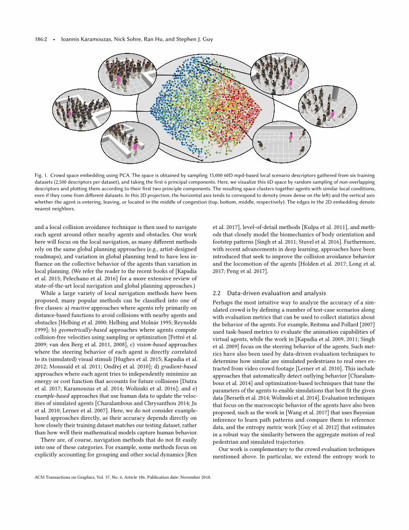
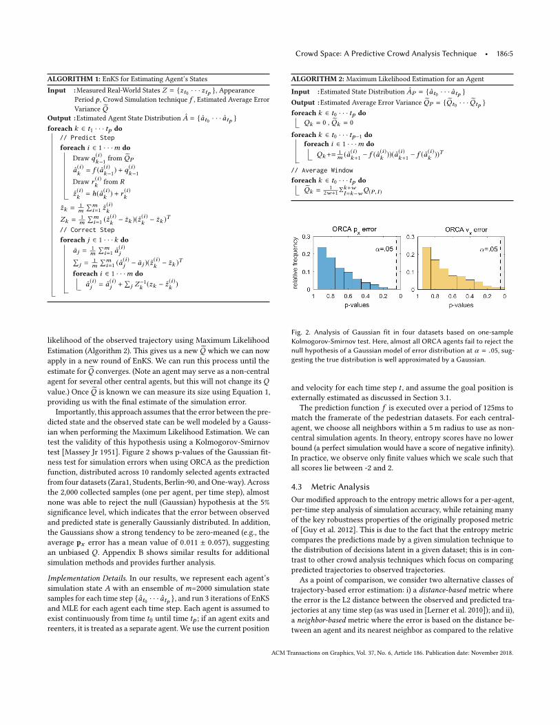
Importantly, this approach assumes that the error between the pre-dicted state and the observed state can be well modeled by a Gauss-ian when performing the Maximum Likelihood Estimation. We cantest the validity of this hypothesis using a Kolmogorov-Smirnovtest [Massey Jr 1951]. Figure 2 shows p-values of the Gaussian fit-ness test for simulation errors when using ORCA as the predictionfunction, distributed across 10 randomly selected agents extractedfrom four datasets (Zara1, Students, Berlin-90, and One-way). Acrossthe 2,000 collected samples (one per agent, per time step), almostnone was able to reject the null (Gaussian) hypothesis at the 5%significance level, which indicates that the error between observedand predicted state is generally Gaussianly distributed. In addition,the Gaussians show a strong tendency to be zero-meaned (e.g., theaverage px error has a mean value of 0.011 ± 0.057), suggestingan unbiased Q . Appendix B shows similar results for additionalsimulation methods and provides further analysis.

Implementation Details. In our results, we represent each agent’ssimulation state A with an ensemble of m=2000 simulation statesamples for each time step {at0 · · · atp }, and run 3 iterations of EnKSand MLE for each agent each time step. Each agent is assumed toexist continuously from time t0 until time tp ; if an agent exits andreenters, it is treated as a separate agent. We use the current position

ALGORITHM 2: Maximum Likelihood Estimation for an Agent

Input :Estimated State Distribution AP = {at0 · · · atp }Output :Estimated Average Error Variance QP = {Qt0 · · · Qtp }foreach k ∈ t0 · · · tp do

Qk = 0 , Qk = 0

foreach k ∈ t0 · · · tp−1 doforeach i ∈ 1 · · ·m do

Qk+=1m (a(i )k+1 − f (a(i )k ))(a(i )k+1 − f (a(i )k ))T

// Average Window

foreach k ∈ t0 · · · tp doQk =

12w+1Σ

k+wI=k−wQ(P, I )

Fig. 2. Analysis of Gaussian fit in four datasets based on one-sampleKolmogorov-Smirnov test. Here, almost all ORCA agents fail to reject thenull hypothesis of a Gaussian model of error distribution at α = .05, sug-gesting the true distribution is well approximated by a Gaussian.

and velocity for each time step t , and assume the goal position isexternally estimated as discussed in Section 3.1.The prediction function f is executed over a period of 125ms to

match the framerate of the pedestrian datasets. For each central-agent, we choose all neighbors within a 5m radius to use as non-central simulation agents. In theory, entropy scores have no lowerbound (a perfect simulation would have a score of negative infinity).In practice, we observe only finite values which we scale such thatall scores lie between -2 and 2.

4.3 Metric AnalysisOur modified approach to the entropy metric allows for a per-agent,per-time step analysis of simulation accuracy, while retaining manyof the key robustness properties of the originally proposed metricof [Guy et al. 2012]. This is due to the fact that the entropy metriccompares the predictions made by a given simulation technique tothe distribution of decisions latent in a given dataset; this is in con-trast to other crowd analysis techniques which focus on comparingpredicted trajectories to observed trajectories.

As a point of comparison, we consider two alternative classes oftrajectory-based error estimation: i) a distance-based metric wherethe error is the L2 distance between the observed and predicted tra-jectories at any time step (as was used in [Lerner et al. 2010]); and ii),a neighbor-based metric where the error is based on the distance be-tween an agent and its nearest neighbor as compared to the relative



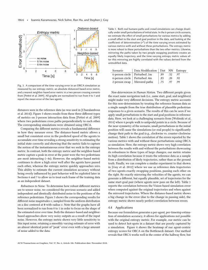
Fig. 3. A comparison of the time-varying error in an ORCA simulation asmeasured by our entropy metric, an absolute distanced-based error metric,and a nearest neighbor-based error metric in a two-person crossing scenariofrom [Pettré et al. 2009]. All graphs are normalized to run from 0 to 1 andreport the mean error of the two agents.

distances seen in the reference data (as was used in [Charalambouset al. 2014]). Figure 3 shows results from these three different typesof metrics on 2-person interaction data from [Pettré et al. 2009]where two pedestrians cross paths perpendicularly to each other.The corresponding simulations were obtained using ORCA.

Comparing the different metrics reveals a fundamental differencein how they measure error. The distance-based metric allows asmall but consistent error in the predicted speed of the agents toaccumulate over time revealing a strong sensitivity to estimating theinitial state correctly and showing that the metric fails to capturethe notion of the instantaneous error that we seek in the entropymetric. In contrast, both the entropy metric and the neighbor-basedmetric capture a peak in error at the point were the two pedestriansare most interacting (∼4s). However, the neighbor-based metriccontinues to show a high error well after the agents have passedeach other, whereas the entropy metric quickly approaches zero.This ability to estimate the current simulation accuracy withoutbeing overly influenced by past behavior will be exploited later inSections 6 and 7 to allow us to treat each frame of the training dataas an independent dataset.

Robustness to Noise. To determine how robust different metricsare to sensor noise, we considered the previous scenario and addedindependent and identically distributed noise to the positions of thereference pedestrians. Figure 3 shows the corresponding results fordifferent noise magnitudesv , sampled from the uniform distributionon a disc centered at 0 with radius v . Note that the graphs have allbeen normalized to run from 0 to 1 in order to focus on the shape ofthe estimated error over time. Both the distance-based and neighbor-based approaches show very noisy outputs as a result of the inputnoise. However, the entropy metric shows very little sensitivity tothis input noise, retaining a smoothly varying estimate of error withan almost identical point of “peak” error even with a large amountof noise added to the data.

Table 1. Both real humans paths and crowd simulations can change drasti-cally under small perturbations of initial state. In the 6-person circle scenario,we estimate the effect of small perturbations for various metrics by addinga small offset to the start and goal position in the data, and looking at thecoefficient of determination (r 2) of the time varying errors estimated byvarious metrics with and without these perturbations. The entropy metricis more robust to these perturbations than the two other metrics. Likewise,mirroring the paths taken by two people swapping positions creates anequally likely trajectory, and the time-varying entropy metric values af-ter this mirroring are highly correlated with the values derived from theunmodified data.

Scenario Data Modification Dist NN Entropy6-person circle Perturbed .1m .89 .52 .976-person circle Perturbed .4m .83 .20 .922-person swap Mirrored paths .75 .97 .99

Non-determinism in Human Motion. Two different people giventhe exact same navigation task (i.e., same start, goal, and neighbors)might make very different decisions. The entropy metric accountsfor this non-determinism by treating the reference human data asa single sample from the true distribution of plausible pedestrianresponses to a given scenario. The results of this can be seen if weapply small perturbations to the start and goal positions in referencedata. Here, we look at a challenging scenario from [Wolinski et al.2014] where 6 people walk to antipodal points in a circle. Because ofthe near-symmetry of the scenario, small perturbations in the initialposition will cause the simulations (or real people) to significantlychange their path to the goal (e.g., clockwise vs. counter-clockwisemotion). Table 1 shows the correlation of the errors reported by thevarious metrics with and without these perturbations using ORCAas simulation. Here, the entropy metric shows very high correlationbetween the results with and without the perturbations showcasingits robustness to these types of large changes; our metric retainsits high correlation because it treats the reference data as a samplefrom a distribution of likely trajectories, rather than as the groundtruth. Finally, we can complete a similar experiment to that shownin [Guy et al. 2012] where we use as reference data trajectoriesof two agents exactly swapping positions, passing each other onthe right. By exactly mirroring the velocities of the agents, we cangenerate a different, but equally plausible, set of trajectories for thesame start-goal pair (where agents now pass on the left). Table 1reports the correlation between the Vision-based simulation errorwhen computed against the original trajectories and when againstthe mirrored trajectories. Where the distance-based metric showsa big change in the error (due to the change in passing side), theentropy metric shows nearly perfect correlation between errors.

4.4 ApplicationsBecause our formulation generates a per-agent, per-timestep estima-tion of simulation accuracy, it allows for applications not possiblewith the original entropy metric. For example, our metric can beused to detect hot-spots in a dataset that are poorly captured bya simulation. Figure 4 shows the heatmap of our agent-centricentropy scores for ORCA on the Bottleneck dataset. Our methodreveals that ORCA works well in the center of the hallway flow, but



-1

-0.5

0

0.5

1

1.5

Entropy

Bottleneck dataset - ORCA

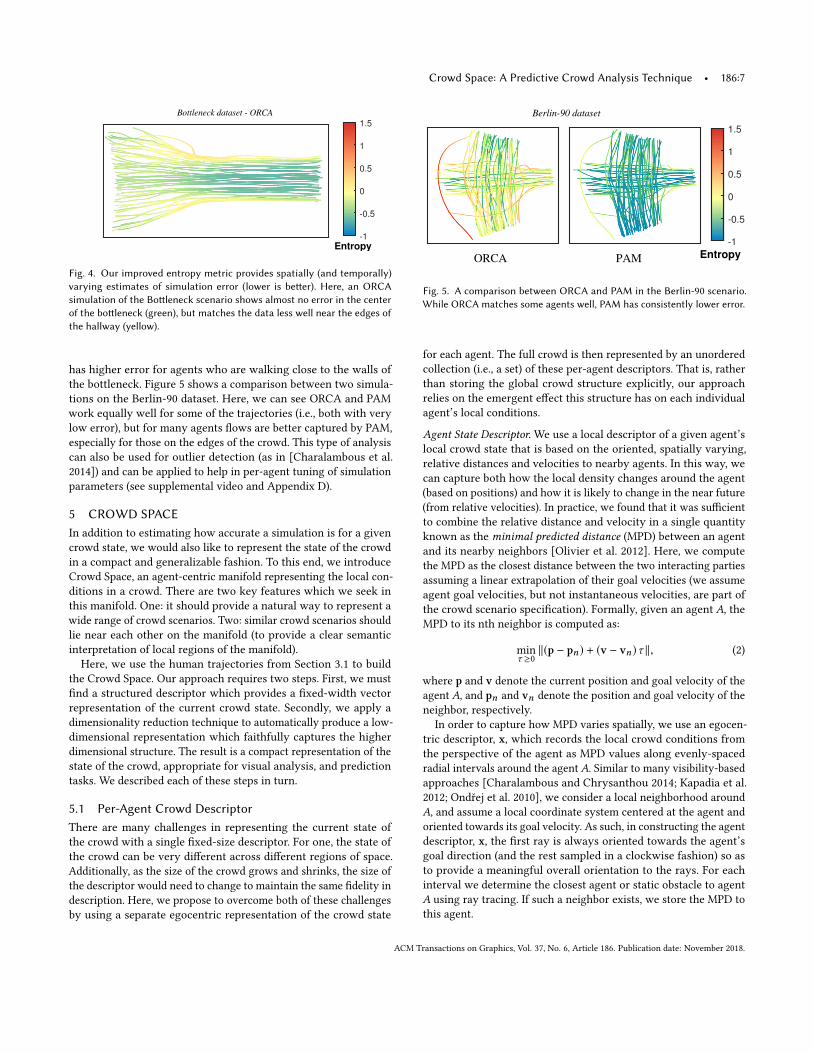
Fig. 4. Our improved entropy metric provides spatially (and temporally)varying estimates of simulation error (lower is better). Here, an ORCAsimulation of the Bottleneck scenario shows almost no error in the centerof the bottleneck (green), but matches the data less well near the edges ofthe hallway (yellow).

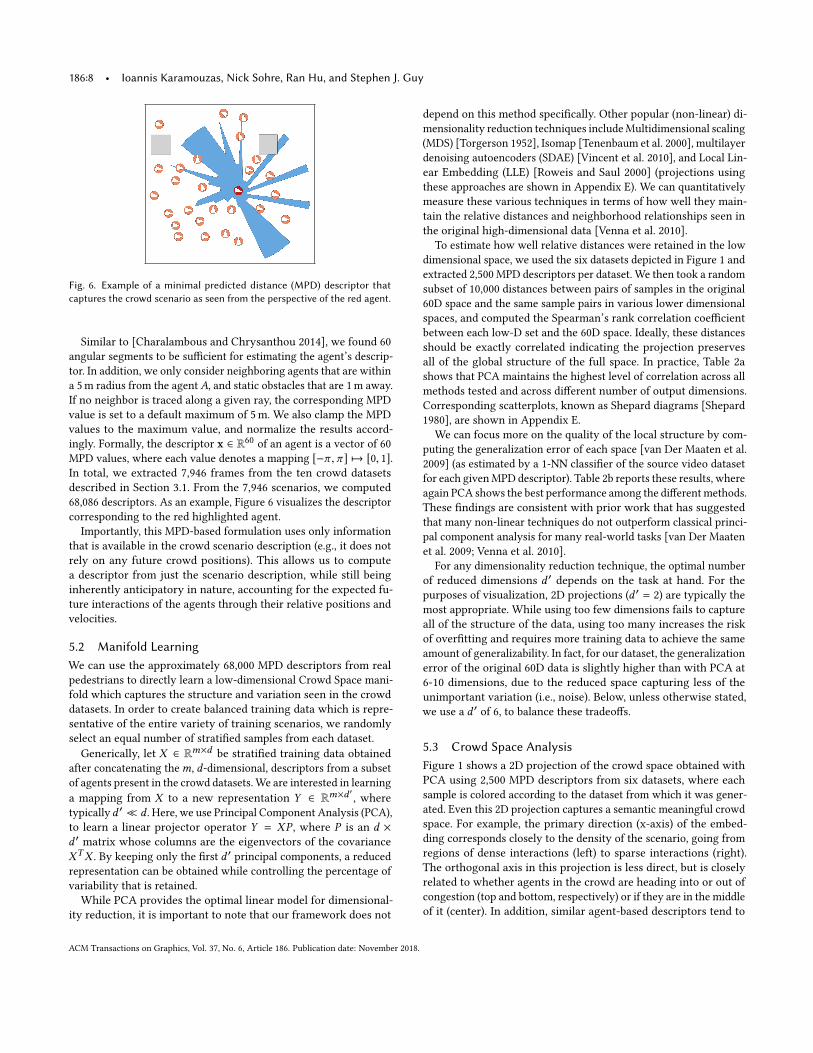
has higher error for agents who are walking close to the walls ofthe bottleneck. Figure 5 shows a comparison between two simula-tions on the Berlin-90 dataset. Here, we can see ORCA and PAMwork equally well for some of the trajectories (i.e., both with verylow error), but for many agents flows are better captured by PAM,especially for those on the edges of the crowd. This type of analysiscan also be used for outlier detection (as in [Charalambous et al.2014]) and can be applied to help in per-agent tuning of simulationparameters (see supplemental video and Appendix D).

5 CROWD SPACEIn addition to estimating how accurate a simulation is for a givencrowd state, we would also like to represent the state of the crowdin a compact and generalizable fashion. To this end, we introduceCrowd Space, an agent-centric manifold representing the local con-ditions in a crowd. There are two key features which we seek inthis manifold. One: it should provide a natural way to represent awide range of crowd scenarios. Two: similar crowd scenarios shouldlie near each other on the manifold (to provide a clear semanticinterpretation of local regions of the manifold).Here, we use the human trajectories from Section 3.1 to build

the Crowd Space. Our approach requires two steps. First, we mustfind a structured descriptor which provides a fixed-width vectorrepresentation of the current crowd state. Secondly, we apply adimensionality reduction technique to automatically produce a low-dimensional representation which faithfully captures the higherdimensional structure. The result is a compact representation of thestate of the crowd, appropriate for visual analysis, and predictiontasks. We described each of these steps in turn.

5.1 Per-Agent Crowd DescriptorThere are many challenges in representing the current state ofthe crowd with a single fixed-size descriptor. For one, the state ofthe crowd can be very different across different regions of space.Additionally, as the size of the crowd grows and shrinks, the size ofthe descriptor would need to change to maintain the same fidelity indescription. Here, we propose to overcome both of these challengesby using a separate egocentric representation of the crowd state

-1

-0.5

0

0.5

1

1.5

PAM Entropy

Berlin-90 dataset

ORCA

Fig. 5. A comparison between ORCA and PAM in the Berlin-90 scenario.While ORCA matches some agents well, PAM has consistently lower error.

for each agent. The full crowd is then represented by an unorderedcollection (i.e., a set) of these per-agent descriptors. That is, ratherthan storing the global crowd structure explicitly, our approachrelies on the emergent effect this structure has on each individualagent’s local conditions.

Agent State Descriptor.We use a local descriptor of a given agent’slocal crowd state that is based on the oriented, spatially varying,relative distances and velocities to nearby agents. In this way, wecan capture both how the local density changes around the agent(based on positions) and how it is likely to change in the near future(from relative velocities). In practice, we found that it was sufficientto combine the relative distance and velocity in a single quantityknown as the minimal predicted distance (MPD) between an agentand its nearby neighbors [Olivier et al. 2012]. Here, we computethe MPD as the closest distance between the two interacting partiesassuming a linear extrapolation of their goal velocities (we assumeagent goal velocities, but not instantaneous velocities, are part ofthe crowd scenario specification). Formally, given an agent A, theMPD to its nth neighbor is computed as:

minτ ≥0

∥(p − pn ) + (v − vn )τ ∥, (2)

where p and v denote the current position and goal velocity of theagent A, and pn and vn denote the position and goal velocity of theneighbor, respectively.

In order to capture how MPD varies spatially, we use an egocen-tric descriptor, x, which records the local crowd conditions fromthe perspective of the agent as MPD values along evenly-spacedradial intervals around the agent A. Similar to many visibility-basedapproaches [Charalambous and Chrysanthou 2014; Kapadia et al.2012; Ondřej et al. 2010], we consider a local neighborhood aroundA, and assume a local coordinate system centered at the agent andoriented towards its goal velocity. As such, in constructing the agentdescriptor, x, the first ray is always oriented towards the agent’sgoal direction (and the rest sampled in a clockwise fashion) so asto provide a meaningful overall orientation to the rays. For eachinterval we determine the closest agent or static obstacle to agentA using ray tracing. If such a neighbor exists, we store the MPD tothis agent.



Fig. 6. Example of a minimal predicted distance (MPD) descriptor thatcaptures the crowd scenario as seen from the perspective of the red agent.

Similar to [Charalambous and Chrysanthou 2014], we found 60angular segments to be sufficient for estimating the agent’s descrip-tor. In addition, we only consider neighboring agents that are withina 5m radius from the agentA, and static obstacles that are 1m away.If no neighbor is traced along a given ray, the corresponding MPDvalue is set to a default maximum of 5m. We also clamp the MPDvalues to the maximum value, and normalize the results accord-ingly. Formally, the descriptor x ∈ R60 of an agent is a vector of 60MPD values, where each value denotes a mapping [−π ,π ] 7→ [0, 1].In total, we extracted 7,946 frames from the ten crowd datasetsdescribed in Section 3.1. From the 7,946 scenarios, we computed68,086 descriptors. As an example, Figure 6 visualizes the descriptorcorresponding to the red highlighted agent.

Importantly, this MPD-based formulation uses only informationthat is available in the crowd scenario description (e.g., it does notrely on any future crowd positions). This allows us to computea descriptor from just the scenario description, while still beinginherently anticipatory in nature, accounting for the expected fu-ture interactions of the agents through their relative positions andvelocities.

5.2 Manifold LearningWe can use the approximately 68,000 MPD descriptors from realpedestrians to directly learn a low-dimensional Crowd Space mani-fold which captures the structure and variation seen in the crowddatasets. In order to create balanced training data which is repre-sentative of the entire variety of training scenarios, we randomlyselect an equal number of stratified samples from each dataset.Generically, let X ∈ Rm×d be stratified training data obtained

after concatenating them, d-dimensional, descriptors from a subsetof agents present in the crowd datasets. We are interested in learninga mapping from X to a new representation Y ∈ Rm×d ′

, wheretypicallyd ′ ≪ d . Here, we use Principal Component Analysis (PCA),to learn a linear projector operator Y = XP , where P is an d ×d ′ matrix whose columns are the eigenvectors of the covarianceXTX . By keeping only the first d ′ principal components, a reducedrepresentation can be obtained while controlling the percentage ofvariability that is retained.

While PCA provides the optimal linear model for dimensional-ity reduction, it is important to note that our framework does not

depend on this method specifically. Other popular (non-linear) di-mensionality reduction techniques includeMultidimensional scaling(MDS) [Torgerson 1952], Isomap [Tenenbaum et al. 2000], multilayerdenoising autoencoders (SDAE) [Vincent et al. 2010], and Local Lin-ear Embedding (LLE) [Roweis and Saul 2000] (projections usingthese approaches are shown in Appendix E). We can quantitativelymeasure these various techniques in terms of how well they main-tain the relative distances and neighborhood relationships seen inthe original high-dimensional data [Venna et al. 2010].

To estimate how well relative distances were retained in the lowdimensional space, we used the six datasets depicted in Figure 1 andextracted 2,500 MPD descriptors per dataset. We then took a randomsubset of 10,000 distances between pairs of samples in the original60D space and the same sample pairs in various lower dimensionalspaces, and computed the Spearman’s rank correlation coefficientbetween each low-D set and the 60D space. Ideally, these distancesshould be exactly correlated indicating the projection preservesall of the global structure of the full space. In practice, Table 2ashows that PCA maintains the highest level of correlation across allmethods tested and across different number of output dimensions.Corresponding scatterplots, known as Shepard diagrams [Shepard1980], are shown in Appendix E.

We can focus more on the quality of the local structure by com-puting the generalization error of each space [van Der Maaten et al.2009] (as estimated by a 1-NN classifier of the source video datasetfor each givenMPD descriptor). Table 2b reports these results, whereagain PCA shows the best performance among the different methods.These findings are consistent with prior work that has suggestedthat many non-linear techniques do not outperform classical princi-pal component analysis for many real-world tasks [van Der Maatenet al. 2009; Venna et al. 2010].

For any dimensionality reduction technique, the optimal numberof reduced dimensions d ′ depends on the task at hand. For thepurposes of visualization, 2D projections (d ′ = 2) are typically themost appropriate. While using too few dimensions fails to captureall of the structure of the data, using too many increases the riskof overfitting and requires more training data to achieve the sameamount of generalizability. In fact, for our dataset, the generalizationerror of the original 60D data is slightly higher than with PCA at6-10 dimensions, due to the reduced space capturing less of theunimportant variation (i.e., noise). Below, unless otherwise stated,we use a d ′ of 6, to balance these tradeoffs.

5.3 Crowd Space AnalysisFigure 1 shows a 2D projection of the crowd space obtained withPCA using 2,500 MPD descriptors from six datasets, where eachsample is colored according to the dataset from which it was gener-ated. Even this 2D projection captures a semantic meaningful crowdspace. For example, the primary direction (x-axis) of the embed-ding corresponds closely to the density of the scenario, going fromregions of dense interactions (left) to sparse interactions (right).The orthogonal axis in this projection is less direct, but is closelyrelated to whether agents in the crowd are heading into or out ofcongestion (top and bottom, respectively) or if they are in the middleof it (center). In addition, similar agent-based descriptors tend to



Table 2. Analysis of various dimensionality reduction techniques at different numbers of output dimensions. (a) Rank-correlation analysis of how well thereduced space preserves the (high-dimensional) distances between data points. (b) The generalization error as measured by 1-NN video dataset misclassificationrate. For both metrics, PCA performs the best across all output dimensions.

(a) Distance Correlations (higher is better)

# Dim. PCA SDAE MDS Isomap LLE2D .931 .824 .896 .925 .4786D .975 .963 .931 .970 .34710D .985 .956 .944 .971 .256

(b) Generalization Error (lower is better)

# Dim. PCA SDAE MDS Isomap LLE2D .442 .464 .474 .448 .5246D .152 .232 .542 .213 .37610D .113 .200 .545 .196 .326

naturally cluster together independent of the crowd dataset theycame from, indicating the ability of our linear projector to learn thehigh-dimensional structure of the MPD-based input data.

Classification Accuracy.We can quantify howwell the derived CrowdSpace captures high-level, semantically meaningful informationabout the structure of the crowd, by training a k-nearest neighbors(k-NN) classifier using this space. Here, we use the label of whichdataset a given MPD descriptor came from as training. Becausenearby descriptors in a (smooth) low-D space should share consis-tent labels, a neighbor-based classifier should be able to reliablylabel novel samples with high accuracy.

Formally, given a scenario descriptor I = {x1, . . . , xn } (i.e., con-sisting of n per-agent MPD descriptors), we need to predict itsdataset label y which can take one of K different known values. Todo so, we need to estimate the probability p(yj = 1 | P ,I) for eachj ∈ [1,K]. Since the scenario consists of n agents, we use a pluralityvoting scheme to determine such probability (relying on a maximumlikelihood assumption). In particular, we use the learned operatorP to project each agent descriptor xi ∈ I to the PCA crowd spaceand identify its k-closest training examples. The most representeddataset label by the k × n nearest neighbors is considered as the I’spredicted dataset label.

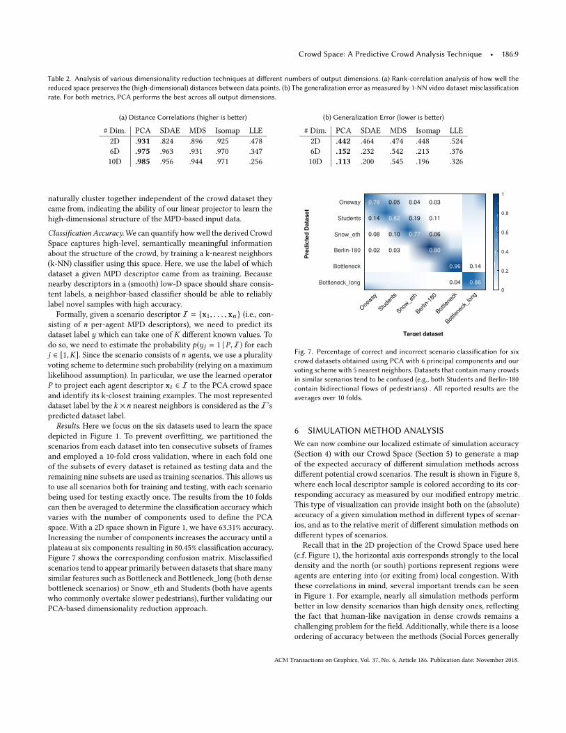
Results. Here we focus on the six datasets used to learn the spacedepicted in Figure 1. To prevent overfitting, we partitioned thescenarios from each dataset into ten consecutive subsets of framesand employed a 10-fold cross validation, where in each fold oneof the subsets of every dataset is retained as testing data and theremaining nine subsets are used as training scenarios. This allows usto use all scenarios both for training and testing, with each scenariobeing used for testing exactly once. The results from the 10 foldscan then be averaged to determine the classification accuracy whichvaries with the number of components used to define the PCAspace. With a 2D space shown in Figure 1, we have 63.31% accuracy.Increasing the number of components increases the accuracy until aplateau at six components resulting in 80.45% classification accuracy.Figure 7 shows the corresponding confusion matrix. Misclassifiedscenarios tend to appear primarily between datasets that share manysimilar features such as Bottleneck and Bottleneck_long (both densebottleneck scenarios) or Snow_eth and Students (both have agentswho commonly overtake slower pedestrians), further validating ourPCA-based dimensionality reduction approach.

0.14

0.86

0.96

0.04

0.03

0.11

0.06

0.80

0.04

0.19

0.77

0.05

0.82

0.10

0.03

0.76

0.14

0.08

0.02

Pre

dic

ted

Data

set

One

way

Stude

nts

Snow_e

th

Berlin

-180

Bottle

neck

Bottle

neck

_lon

g

Oneway

Students

Snow_eth

Berlin-180

Bottleneck

Bottleneck_long

0

0.2

0.4

0.6

0.8

1

Target dataset

Fig. 7. Percentage of correct and incorrect scenario classification for sixcrowd datasets obtained using PCA with 6 principal components and ourvoting scheme with 5 nearest neighbors. Datasets that contain many crowdsin similar scenarios tend to be confused (e.g., both Students and Berlin-180contain bidirectional flows of pedestrians) . All reported results are theaverages over 10 folds.

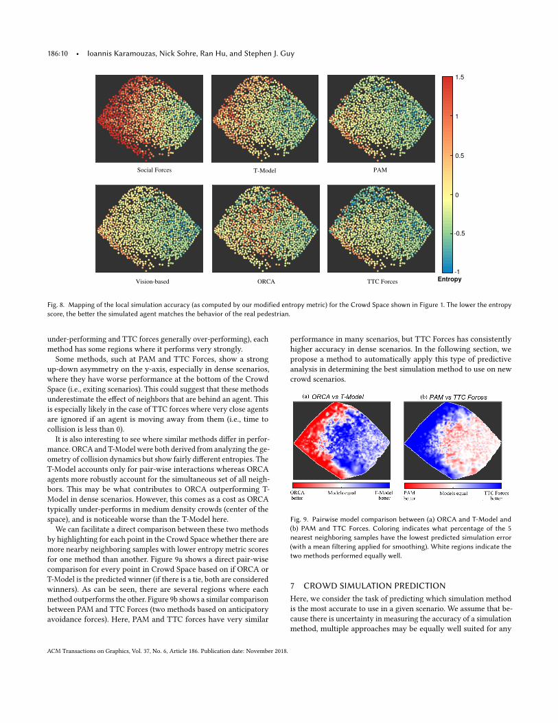
6 SIMULATION METHOD ANALYSISWe can now combine our localized estimate of simulation accuracy(Section 4) with our Crowd Space (Section 5) to generate a mapof the expected accuracy of different simulation methods acrossdifferent potential crowd scenarios. The result is shown in Figure 8,where each local descriptor sample is colored according to its cor-responding accuracy as measured by our modified entropy metric.This type of visualization can provide insight both on the (absolute)accuracy of a given simulation method in different types of scenar-ios, and as to the relative merit of different simulation methods ondifferent types of scenarios.Recall that in the 2D projection of the Crowd Space used here

(c.f. Figure 1), the horizontal axis corresponds strongly to the localdensity and the north (or south) portions represent regions wereagents are entering into (or exiting from) local congestion. Withthese correlations in mind, several important trends can be seenin Figure 1. For example, nearly all simulation methods performbetter in low density scenarios than high density ones, reflectingthe fact that human-like navigation in dense crowds remains achallenging problem for the field. Additionally, while there is a looseordering of accuracy between the methods (Social Forces generally



0

0.5

1

1.5

-0.5

Entropy

PAMSocial Forces T-Model

ORCA TTC ForcesVision-based

-1

Fig. 8. Mapping of the local simulation accuracy (as computed by our modified entropy metric) for the Crowd Space shown in Figure 1. The lower the entropyscore, the better the simulated agent matches the behavior of the real pedestrian.

under-performing and TTC forces generally over-performing), eachmethod has some regions where it performs very strongly.Some methods, such at PAM and TTC Forces, show a strong

up-down asymmetry on the y-axis, especially in dense scenarios,where they have worse performance at the bottom of the CrowdSpace (i.e., exiting scenarios). This could suggest that these methodsunderestimate the effect of neighbors that are behind an agent. Thisis especially likely in the case of TTC forces where very close agentsare ignored if an agent is moving away from them (i.e., time tocollision is less than 0).

It is also interesting to see where similar methods differ in perfor-mance. ORCA and T-Model were both derived from analyzing the ge-ometry of collision dynamics but show fairly different entropies. TheT-Model accounts only for pair-wise interactions whereas ORCAagents more robustly account for the simultaneous set of all neigh-bors. This may be what contributes to ORCA outperforming T-Model in dense scenarios. However, this comes as a cost as ORCAtypically under-performs in medium density crowds (center of thespace), and is noticeable worse than the T-Model here.

We can facilitate a direct comparison between these two methodsby highlighting for each point in the Crowd Space whether there aremore nearby neighboring samples with lower entropy metric scoresfor one method than another. Figure 9a shows a direct pair-wisecomparison for every point in Crowd Space based on if ORCA orT-Model is the predicted winner (if there is a tie, both are consideredwinners). As can be seen, there are several regions where eachmethod outperforms the other. Figure 9b shows a similar comparisonbetween PAM and TTC Forces (two methods based on anticipatoryavoidance forces). Here, PAM and TTC forces have very similar

performance in many scenarios, but TTC Forces has consistentlyhigher accuracy in dense scenarios. In the following section, wepropose a method to automatically apply this type of predictiveanalysis in determining the best simulation method to use on newcrowd scenarios.

Fig. 9. Pairwise model comparison between (a) ORCA and T-Model and(b) PAM and TTC Forces. Coloring indicates what percentage of the 5nearest neighboring samples have the lowest predicted simulation error(with a mean filtering applied for smoothing). White regions indicate thetwo methods performed equally well.

7 CROWD SIMULATION PREDICTIONHere, we consider the task of predicting which simulation methodis the most accurate to use in a given scenario. We assume that be-cause there is uncertainty in measuring the accuracy of a simulationmethod, multiple approaches may be equally well suited for any



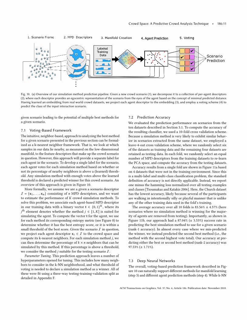
Fig. 10. (a) Overview of our simulation method prediction pipeline. Given a new crowd scenario (1), we decompose it to a collection of per-agent descriptors(2), where each descriptor provides an egocentric representation of the scenario from the eyes of the agent based on the concept of minimal predicted distance.Having learned an embedding from real world crowd datasets, we project each agent descriptor to the embedding (3), and employ a voting scheme (4) topredict the class of the input interaction scenario.

given scenario leading to the potential of multiple best methods fora given scenario.

7.1 Voting-Based FrameworkThe intuitive, neighbor-based, approach to analyzing the bestmethodfor a given scenario presented in the previous section can be formal-ized as a k-nearest neighbor framework. That is, we look at whichsamples in our data lie nearby, as measured on the low-dimensionalmanifold, to the feature descriptors that make up the crowd scenarioin question. However, this approach will provide a separate label foreach agent in the scenario. To develop a single label for the scenario,each agent votes for each simulation method based on whether ornot its percentage of nearby neighbors is above a (learned) thresh-old. Any simulation method with enough votes above the learnedthreshold is declared a predicted winner for this crowd scenario. Anoverview of this approach is given in Figure 10.More formally, we assume we are a given a scenario descriptor

I = {x1, . . . , xn } consisting of n MPD descriptors, and we wantto estimate the performance of K crowd simulation methods. Tosolve this problem, we associate each agent-based MPD descriptorin our training data with a binary vector t ∈ {0, 1}K , where itsjth element denotes whether the method j ∈ [1,K] is suited forsimulating the agent. To compute the vector t for the agent, we usefor each method its corresponding entropy metric (see Figure 8) todetermine whether it has the best entropy score, or it is within asmall threshold of the best score. Given the scenario I in question,we project each agent descriptor xi ∈ I to the crowd space andcompute its k-nearest neighbors. For each simulation method j, wecan then determine the percentage of k × n neighbors that can besimulated by this method. If this percentage is above a threshold,we consider the method j suitable for the testing scenario I.

Parameter Tuning. This prediction approach leaves a number ofhyperparameters opened for tuning. This includes how many neigh-bors to consider in the k-NN neighborhood, and what threshold ofvoting is needed to declare a simulation method as a winner. All ofthese were fit using a three-way testing-training-validation split asdetailed in Appendix F.

7.2 Prediction AccuracyWe evaluated the prediction performance on scenarios from theten datasets described in Section 3.1. To compute the accuracy ofthe resulting classifier, we used a 10-fold cross validation scheme.Because a simulation method is very likely to exhibit similar behav-ior in scenarios extracted from the same dataset, we employed aleave-4-out cross validation scheme, where we randomly select sixof the datasets as training data and the remaining four datasets areretained as testing data. In each fold, we randomly select an equalnumber of MPD descriptors from the training datasets to re-learnthe PCA space, and compute the accuracy from the testing datasets.

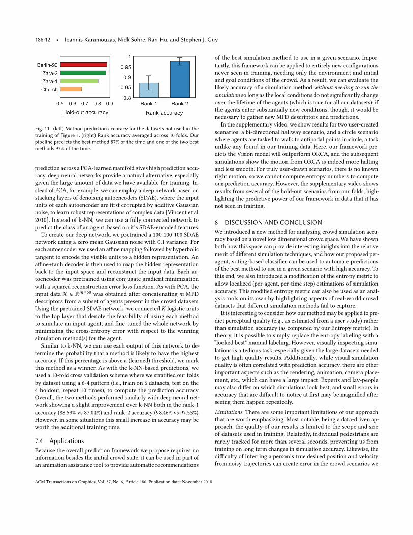
Accuracy results from a single fold are shown in Figure 11a basedon 4 datasets that were not in the training environment. Since thisis a multi-label and multi-class classification problem, the standarddefinition of accuracy is not directly applicable. Instead, we reportone minus the hamming loss normalized over all testing examplesand classes [Tsoumakas and Katakis 2006]. Here, the Church datasethas the lowest accuracy, likely because several of the participantsare walking in intentionally silly or playful manner that is unlikeany of the other training data used in the fold’s training.The average accuracy over all 10 folds is 83.56% ± 4.57% (here

scenarios where no simulation method is winning for the major-ity of agents are removed from testing). Importantly, as shown inFigure 11b, our approach had a 87.04% (± 3.53%) success rate inpredicting the best simulation method to use for a given scenario(rank-1 accuracy). In almost every case where we mis-predictedthe winner, we instead predicted the second best method (i.e., themethod with the second highest vote total). Our accuracy at pre-dicting either the best or second best method (rank-2 accuracy) was97.53% (± 1.71%).

7.3 Deep Neural NetworksThe overall, voting-based prediction framework described in Fig-ure 10 can naturally support different methods for manifold learning(step 3) and different agent prediction methods (step 4). While k-NN



Fig. 11. (left) Method prediction accuracy for the datasets not used in thetraining of Figure 1. (right) Rank accuracy averaged across 10 folds. Ourpipeline predicts the best method 87% of the time and one of the two bestmethods 97% of the time.

prediction across a PCA-learnedmanifold gives high prediction accu-racy, deep neural networks provide a natural alternative, especiallygiven the large amount of data we have available for training. In-stead of PCA, for example, we can employ a deep network based onstacking layers of denoising autoencoders (SDAE), where the inputunits of each autoencoder are first corrupted by additive Gaussiannoise, to learn robust representations of complex data [Vincent et al.2010]. Instead of k-NN, we can use a fully connected network topredict the class of an agent, based on it’s SDAE-encoded features.To create our deep network, we pretrained a 100-100-100 SDAE

network using a zero mean Gaussian noise with 0.1 variance. Foreach autoencoder we used an affine mapping followed by hyperbolictangent to encode the visible units to a hidden representation. Anaffine+tanh decoder is then used to map the hidden representationback to the input space and reconstruct the input data. Each au-toencoder was pretrained using conjugate gradient minimizationwith a squared reconstruction error loss function. As with PCA, theinput data X ∈ Rm×60 was obtained after concatenatingm MPDdescriptors from a subset of agents present in the crowd datasets.Using the pretrained SDAE network, we connected K logistic unitsto the top layer that denote the feasibility of using each methodto simulate an input agent, and fine-tuned the whole network byminimizing the cross-entropy error with respect to the winningsimulation method(s) for the agent.Similar to k-NN, we can use each output of this network to de-

termine the probability that a method is likely to have the highestaccuracy. If this percentage is above a (learned) threshold, we markthis method as a winner. As with the k-NN-based predictions, weused a 10-fold cross validation scheme where we stratified our foldsby dataset using a 6-4 pattern (i.e., train on 6 datasets, test on the4 holdout, repeat 10 times), to compute the prediction accuracy.Overall, the two methods performed similarly with deep neural net-work showing a slight improvement over k-NN both in the rank-1accuracy (88.59% vs 87.04%) and rank-2 accuracy (98.46% vs 97.53%).However, in some situations this small increase in accuracy may beworth the additional training time.

7.4 ApplicationsBecause the overall prediction framework we propose requires noinformation besides the initial crowd state, it can be used in part ofan animation assistance tool to provide automatic recommendations

of the best simulation method to use in a given scenario. Impor-tantly, this framework can be applied to entirely new configurationsnever seen in training, needing only the environment and initialand goal conditions of the crowd. As a result, we can evaluate thelikely accuracy of a simulation method without needing to run thesimulation so long as the local conditions do not significantly changeover the lifetime of the agents (which is true for all our datasets); ifthe agents enter substantially new conditions, though, it would benecessary to gather new MPD descriptors and predictions.

In the supplementary video, we show results for two user-createdscenarios: a bi-directional hallway scenario, and a circle scenariowhere agents are tasked to walk to antipodal points in circle, a taskunlike any found in our training data. Here, our framework pre-dicts the Vision model will outperform ORCA, and the subsequentsimulations show the motion from ORCA is indeed more haltingand less smooth. For truly user-drawn scenarios, there is no knownright motion, so we cannot compute entropy numbers to computeour prediction accuracy. However, the supplementary video showsresults from several of the hold-out scenarios from our folds, high-lighting the predictive power of our framework in data that it hasnot seen in training.

8 DISCUSSION AND CONCLUSIONWe introduced a new method for analyzing crowd simulation accu-racy based on a novel low dimensional crowd space. We have shownboth how this space can provide interesting insights into the relativemerit of different simulation techniques, and how our proposed per-agent, voting-based classifier can be used to automate predictionsof the best method to use in a given scenario with high accuracy. Tothis end, we also introduced a modification of the entropy metric toallow localized (per-agent, per-time step) estimations of simulationaccuracy. This modified entropy metric can also be used as an anal-ysis tools on its own by highlighting aspects of real-world crowddatasets that different simulation methods fail to capture.

It is interesting to consider how our methodmay be applied to pre-dict perceptual quality (e.g., as estimated from a user study) ratherthan simulation accuracy (as computed by our Entropy metric). Intheory, it is possible to simply replace the entropy labeling with a“looked best" manual labeling. However, visually inspecting simu-lations is a tedious task, especially given the large datasets neededto get high-quality results. Additionally, while visual simulationquality is often correlated with prediction accuracy, there are otherimportant aspects such as the rendering, animation, camera place-ment, etc., which can have a large impact. Experts and lay-peoplemay also differ on which simulations look best, and small errors inaccuracy that are difficult to notice at first may be magnified afterseeing them happen repeatedly.Limitations. There are some important limitations of our approachthat are worth emphasizing. Most notable, being a data-driven ap-proach, the quality of our results is limited to the scope and sizeof datasets used in training. Relatedly, individual pedestrians arerarely tracked for more than several seconds, preventing us fromtraining on long term changes in simulation accuracy. Likewise, thedifficulty of inferring a person’s true desired position and velocityfrom noisy trajectories can create error in the crowd scenarios we



extract from the tracked pedestrian datasets. In terms of the learn-ing approach, our descriptor of a crowd scenario is broken into anunstructured collection of per-agent, MPD-based descriptors. Thisrepresentation can lose some of the long-range structure inherentin certain scenarios.Additionally, our proposed voting-based framework treats each

agent equally, which can dampen the effect of extreme outliers(e.g., the negative effect of a small number of very poorly simu-lated agents can be underestimated). Overall, the high accuracy ofour approach suggest these issues had only a limited effect on thescenarios contained in our datasets, but there are of course manyother important simulation scenarios than those we were able totest. Another limitation stems from what is being measured as accu-racy through the entropy metric. The statistical approach used herecan be biased in favor of methods that predict the correct averagebehavior but fail to capture some of the interesting (though unusual)deviations from average.Future work. Looking forward, we see many possibilities for expand-ing the scope of this work and increasing its potential impact. Inaddition to using the Crowd Space to predict simulation accuracy(as measured by the modified entropy metric), we can look at otherimportant measures of quality such as path smoothness, energyminimization, or number of collisions. A similar manifold-basedapproach might also be applicable to other domains where multiplecompeting simulation methods are popular such as character ani-mations or modeling the motion of plants and animals. Though, tobe useful, there would need to exist large datasets of reference realworld motions.

We also hope to address some of the above limitations in fu-ture work. In particular, ideas from object recognition which usemulti-scale, image-based (i.e., sampling-based) feature descriptorsto represent objects at different scales may also be applied to ex-plicitly capture the structure in crowd simulations. We would alsolike to incorporate additional simulation methods to our framework,such as the recent work in [Wolinski et al. 2016] that provides aprobabilistic collision prediction scheme for the agents. We notethat in our current work we tested the simulation accuracy of sixmethods using their default simulation parameters (as providedin the corresponding papers and/or software libraries). However,besides different methods, our approach can also support the testingof the same method but simulated with different sets of parameters,a mixture of the two, etc. As such, we are excited about the prospectof building a tool which can provide visual analysis and automatedinsights as to the best simulation models to use in various scenarios.Lastly, we are interested in exploring the potential of using our

approach to directly drive a simulation method. This could be inthe form of an AI which chooses a new simulation method foreach frame (or each agent) based on the best option for the currentconditions.

ACKNOWLEDGMENTSWe thank Jan Ondřej for sharing his T-model code, and Rahul Narainfor useful discussions. This work was supported in part by the Na-tional Science Foundation under grants IIS-1748541, CHS-1526693,and CNS-1544887.

REFERENCESTunç Ozan Aydin, Martin Čadík, Karol Myszkowski, and Hans-Peter Seidel. 2010. Video

Quality Assessment for Computer Graphics Applications. ACM Transactions onGraphics 29, 6, Article 161 (2010), 12 pages.

Glen Berseth, Mubbasir Kapadia, Brandon Haworth, and Petros Faloutsos. 2014.SteerFit: Automated Parameter Fitting for Steering Algorithms. In ACM SIG-GRAPH/Eurographics Symposium on Computer Animation. 113–122.

Robert Bridson. 2015. Fluid simulation for computer graphics. CRC Press.Panayiotis Charalambous and Yiorgos Chrysanthou. 2014. The PAG Crowd: A Graph

Based Approach for Efficient Data-Driven Crowd Simulation. Computer GraphicsForum 33, 8 (2014), 95–108.

Panayiotis Charalambous, Ioannis Karamouzas, Stephen J. Guy, and Yiorgos Chrysan-thou. 2014. A Data-Driven Framework for Visual Crowd Analysis. ComputerGraphics Forum 33, 7 (2014), 41–50.

Funda Durupinar, Mubbasir Kapadia, Susan Deutsch, Michael Neff, and Norman I Badler.2017. Perform: Perceptual approach for adding ocean personality to human motionusing laban movement analysis. ACM Transactions on Graphics 36, 1 (2017), 6.

Teófilo Dutra, Ricardo Marques, Joaquim B. Cavalcante-Neto, Creto Augusto Vidal,and Julien Pettré. 2017. Gradient-based steering for vision-based crowd simulationalgorithms. Computer Graphics Forum 36, 2 (2017).

Geir Evensen. 2003. The ensemble Kalman filter: Theoretical formulation and practicalimplementation. Ocean dynamics 53, 4 (2003), 343–367.

Stephen J. Guy and Ioannis Karamouzas. 2015. A Guide to Anticipatory CollisionAvoidance. In Game AI Pro 2: Collected Wisdom of Game AI Professionals, SteveRabin (Ed.). A K Peters/CRC Press, Chapter 19, 195–208.

Stephen J Guy, Jur Van Den Berg, Wenxi Liu, Rynson Lau, Ming C Lin, and DineshManocha. 2012. A statistical similarity measure for aggregate crowd dynamics. ACMTransactions on Graphics (TOG) 31, 6 (2012), 190.

Dirk Helbing, Illés Farkas, and Tamas Vicsek. 2000. Simulating dynamical features ofescape panic. Nature 407, 6803 (2000), 487–490.

Dirk Helbing and Péter Molnár. 1995. Social Force Model for Pedestrian Dynamics.Physical Review E 51 (1995), 4282–4286.

Daniel Holden, Taku Komura, and Jun Saito. 2017. Phase-functioned neural networksfor character control. ACM Transactions on Graphics 36, 4 (2017), 42.

Ludovic Hoyet, Kenneth Ryall, Katja Zibrek, Hwangpil Park, Jehee Lee, Jessica Hodgins,and Carol O’sullivan. 2013. Evaluating the distinctiveness and attractiveness ofhuman motions on realistic virtual bodies. ACM Transactions on Graphics 32, 6(2013), 204.

Rowan Hughes, Jan Ondřej, and John Dingliana. 2015. DAVIS: density-adaptivesynthetic-vision based steering for virtual crowds. InMotion in Games. ACM, 79–84.

Eunjung Ju, Myung Geol Choi, Minji Park, Jehee Lee, Kang Hoon Lee, and ShigeoTakahashi. 2010. Morphable crowds. ACM Transactions on Graphics 29 (2010),140:1–140:10. Issue 6.

Mubbasir Kapadia, Nuria Pelechano, Jan Allbeck, and Norm Badler. 2015. Virtualcrowds: Steps toward behavioral realism. Synthesis Lectures on Visual Computing:Computer Graphics, Animation, Computational Photography, and Imaging 7, 4 (2015),1–270.

Mubbasir Kapadia, Shawn Singh, Brian Allen, Glenn Reinman, and Petros Faloutsos.2009. Steerbug: an interactive framework for specifying and detecting steeringbehaviors. In ACM SIGGRAPH/Eurographics Symposium on Computer Animation.209–216.

Mubbasir Kapadia, Shawn Singh,WilliamHewlett, Glenn Reinman, and Petros Faloutsos.2012. Parallelized egocentric fields for autonomous navigation. The Visual Computer28, 12 (2012), 1209–1227.

Mubbasir Kapadia, Matt Wang, Shawn Singh, Glenn Reinman, and Petros Faloutsos.2011. Scenario space: characterizing coverage, quality, and failure of steering al-gorithms. In ACM SIGGRAPH/Eurographics Symposium on Computer Animation.53–62.

Ioannis Karamouzas, Peter Heil, Pascal van Beek, and Mark H. Overmars. 2009. APredictive Collision Avoidance Model for Pedestrian Simulation. InMotion in Games.41–52.

Ioannis Karamouzas, Brian Skinner, and Stephen J. Guy. 2014. Universal Power LawGoverning Pedestrian Interactions. Physical Review Letters 113 (2014), 238701. Issue23.

Ioannis Karamouzas, Nick Sohre, Rahul Narain, and Stephen J. Guy. 2017. ImplicitCrowds: Optimization Integrator for Robust Crowd Simulation. ACM Transactionson Graphics 36, 4 (2017).

Richard Kulpa, Anne-Hélène Olivierxs, Jan Ondřej, and Julien Pettré. 2011. Impercepti-ble relaxation of collision avoidance constraints in virtual crowds. ACM Transactionson Graphics 30, 6 (2011), 138.

Gregor Lämmel and Matthias Plaue. 2014. Getting out of the way: Collision-avoidingpedestrianmodels compared to the realworld. In Pedestrian and Evacuation Dynamics2012. Springer, 1275–1289.

Jehee Lee. 2010. Introduction to Data-driven Animation: Programming with MotionCapture. In ACM SIGGRAPH ASIA 2010 Courses. Article 4, 50 pages. https://doi.org/10.1145/1900520.1900524


https://doi.org/10.1145/1900520.1900524

https://doi.org/10.1145/1900520.1900524


Alon Lerner, Yiorgos Chrysanthou, and Dani Lischinski. 2007. Crowds by example.Computer Graphics Forum 26 (2007), 655–664.

Alon Lerner, Yiorgos Chrysanthou, Ariel Shamir, and Daniel Cohen-Or. 2010. Context-Dependent Crowd Evaluation. Computer Graphics Forum 29, 7 (2010), 2197–2206.

Pinxin Long, Wenxi Liu, and Jia Pan. 2017. Deep-Learned Collision Avoidance Policyfor Distributed Multiagent Navigation. IEEE Robotics and Automation Letters 2, 2(2017), 656–663.

Frank J Massey Jr. 1951. The Kolmogorov-Smirnov test for goodness of fit. Journal ofthe American statistical Association 46, 253 (1951), 68–78.

Rachel McDonnell, Michéal Larkin, Benjamín Hernández, Isaac Rudomin, and CarolO’Sullivan. 2009. Eye-catching Crowds: Saliency Based Selective Variation. ACMTransactions on Graphics 28, 3, Article 55 (2009), 55:1–55:10 pages.

Mehdi Moussaïd, Dirk Helbing, and Guy Theraulaz. 2011. How simple rules determinepedestrian behavior and crowd disasters. Proceedings of the National Academy ofSciences 108, 17 (2011), 6884–6888.

Rahul Narain, Abhinav Golas, Sean Curtis, and Ming C. Lin. 2009. Aggregate Dynamicsfor Dense Crowd Simulation. ACM Transaction on Graphics 28, 5 (2009), 122:1–122:8.

Anne-Hélène Olivier, Antoine Marin, Armel Crétual, and Julien Pettré. 2012. Mini-mal predicted distance: A common metric for collision avoidance during pairwiseinteractions between walkers. Gait Posture 36, 3 (2012), 399–404.

Jan Ondřej, Julien Pettré, Anne-Hélène Olivier, and Stéphane Donikian. 2010. Asynthetic-vision based steering approach for crowd simulation. ACM Transactionson Graphics 29, 4 (2010), 1–9.

Nuria Pelechano, Jan M Allbeck, Mubbasir Kapadia, and Norman I Badler. 2016. Simu-lating Heterogeneous Crowd with Interactive Behaviors. CRC Press.

Stefano Pellegrini, Andrea Ess, Konrad Schindler, and Luc Van Gool. 2009. You’ll neverwalk alone: Modeling social behavior for multi-target tracking. In IEEE InternationalConference on Computer Vision. 261–268.

Xue Bin Peng, Glen Berseth, KangKang Yin, and Michiel Van De Panne. 2017. Deeploco:Dynamic locomotion skills using hierarchical deep reinforcement learning. ACMTransactions on Graphics 36, 4 (2017), 41.

Julien Pettré, Jan Ondřej, Anne-Hélène Olivier, Armel Crétual, and Stéphane Donikian.2009. Experiment-based Modeling, Simulation and Validation of Interactions be-tween Virtual Walkers. In ACM SIGGRAPH/Eurographics Symposium on ComputerAnimation. 189–198.

Paul S.A. Reitsma and Nancy S. Pollard. 2007. Evaluating motion graphs for characteranimation. ACM Transactions on Graphics 26, 4 (2007), 18.

Zhiguo Ren, Panayiotis Charalambous, Julien Bruneau, Qunsheng Peng, and JulienPettré. 2017. Group Modeling: A Unified Velocity-Based Approach. In ComputerGraphics Forum, Vol. 36. 45–56.

Craig W. Reynolds. 1987. Flocks, herds, and schools: A distributed behavioral model.Computer Graphics 21, 4 (1987), 24–34.

Craig W. Reynolds. 1999. Steering Behaviors For Autonomous Characters. In GameDevelopers Conference. 763–782.

Sam T Roweis and Lawrence K Saul. 2000. Nonlinear dimensionality reduction bylocally linear embedding. science 290, 5500 (2000), 2323–2326.

Armin Seyfried, Oliver Passon, Bernhard Steffen, Maik Boltes, Tobias Rupprecht, andWolfram Klingsch. 2009. New insights into pedestrian flow through bottlenecks.Transportation Science 43, 3 (2009), 395–406.

Roger N Shepard. 1980. Multidimensional scaling, tree-fitting, and clustering. Science210, 4468 (1980), 390–398.

Eftychios Sifakis and Jernej Barbic. 2012. FEM Simulation of 3D Deformable Solids:A Practitioner’s Guide to Theory, Discretization and Model Reduction. In ACMSIGGRAPH 2012 Courses. Article 20, 50 pages.

Shawn Singh, Mubbasir Kapadia, Petros Faloutsos, and Glenn Reinman. 2009. Steer-Bench: a benchmark suite for evaluating steering behaviors. Computer Animationand Virtual Worlds 20, 5-6 (2009), 533–548.

Shawn Singh, Mubbasir Kapadia, Glenn Reinman, and Petros Faloutsos. 2011. Footstepnavigation for dynamic crowds. Computer Animation and Virtual Worlds 22, 2-3(2011), 151–158.

Sybren Stuvel, Nadia Magnenat-Thalmann, Daniel Thalmann, A Frank van der Stappen,and Arjan Egges. 2016. Torso Crowds. IEEE Transactions on Visualization andComputer Graphics (2016).

Joshua B Tenenbaum, Vin De Silva, and John C Langford. 2000. A global geometricframework for nonlinear dimensionality reduction. science 290, 5500 (2000), 2319–2323.

Warren S Torgerson. 1952. Multidimensional scaling: I. Theory and method. Psychome-trika 17, 4 (1952), 401–419.

Adrien Treuille, Seth Cooper, and Zoran Popović. 2006. Continuum crowds. ACMTransactions on Graphics 25, 3 (2006), 1160–1168.

Grigorios Tsoumakas and Ioannis Katakis. 2006. Multi-label classification: An overview.International Journal of Data Warehousing and Mining 3, 3 (2006).

Kiwon Um, Xiangyu Hu, and Nils Thuerey. 2017. Perceptual Evaluation of LiquidSimulation Methods. ACM Transactions on Graphics 36, 4, Article 143 (2017), 143:1–143:12 pages. https://doi.org/10.1145/3072959.3073633

Jur van den Berg, Stephen J. Guy, Ming C. Lin, and Dinesh Manocha. 2011. Reciprocaln-body Collision Avoidance. In International Symposium of Robotics Research. 3–19.

Jur van den Berg, Ming C. Lin, and DineshManocha. 2008. Reciprocal Velocity Obstaclesfor real-time multi-agent navigation. In IEEE International Conference on Roboticsand Automation. 1928–1935.

Laurens van Der Maaten, Eric Postma, and Jaap Van den Herik. 2009. Dimensionalityreduction: a comparative review. Journal of Machine Learning Research 10 (2009),66–71.

Jarkko Venna, Jaakko Peltonen, Kristian Nybo, Helena Aidos, and Samuel Kaski. 2010.Information retrieval perspective to nonlinear dimensionality reduction for datavisualization. Journal of Machine Learning Research 11 (2010), 451–490.

Pascal Vincent, Hugo Larochelle, Isabelle Lajoie, Yoshua Bengio, and Pierre-AntoineManzagol. 2010. Stacked denoising autoencoders: Learning useful representationsin a deep network with a local denoising criterion. Journal of Machine LearningResearch 11, Dec (2010), 3371–3408.

He Wang, Jan Ondrej, and Carol O’Sullivan. 2017. Trending Paths: A New Semantic-Level Metric for Comparing Simulated and Real Crowd Data. IEEE Transactions onVisualization & Computer Graphics 23, 5 (2017), 1454–1464.

David Wolinski, Stephen Guy, Anne-Hélène Olivier, Ming Lin, Dinesh Manocha, andJulien Pettré. 2014. Parameter Estimation and Comparative Evaluation of CrowdSimulations. Computer Graphics Forum 33, 2 (2014), 303–312.

David Wolinski, Ming C. Lin, and Julien Pettré. 2016. WarpDriver: context-awareprobabilistic motion prediction for crowd simulation. ACM Transactions on Graphics35, 6 (2016), 164.


https://doi.org/10.1145/3072959.3073633

crowd space: a predictive crowd analysis techniqueioannis/crowd-space/files/crowdspa… · crowd...

Documents