crustal deformation in great california earthquake...

JOURNAL OF GEOPHYSICAL RESEARCH, VOL. 92, NO. Bll, PAGES 11,533-11,551, OCTOBER 10, 1987

Crustal Deformation in Great California Earthquake Cycles

VICTOR C. LI

Department of Civil Engineering, Massachusetts Institute of Technology, Cambridge

JAMES R. RICE

Division of Applied Science and Department of Earth and Planetary Sciences Harvard University, Cambridge, Massachusetts

Periodic crustal deformation associated with repeated strike-slip earthquakes is computed for the following model; A depth L (< H) extending downward from the Earth's surface at a transform boundary between uniform elastic lithospheric plates of thickness H is locked between earthquakes. It slips an amount consistent with remote plate velocity Vp• after each lapse of earthquake cycle time Tcy. Lower portions of the fault zone at the boundary slip continuously so as to maintain constant resistive shear stress. The plates are coupled at their base to a Maxwellian viscoelastic asthenosphere through which steady deep-seated mantle motions, compatible with plate velocity, are transmitted to the surface plates. The coupling is described approximately through a generalized Elsasser model. We argue that the model gives a more realistic physical description of tectonic loading, including the time dependence of deep slip and crustal stress buildup throughout the earthquake cycle, than do simpler kinematic models in which loading is represented as imposed uniform dislocation slip on the fault below the locked zone. Parame- ters of the model are chosen to fit seismic and geologic constraints and the apparent time dependence of surface strain rates along presently locked traces of the 1857 and 1906 San Andreas ruptures. We fix Vp• - 35 mm/yr, rcy= 160 years, and L - 9-11 km based on earthquake nucleation depths. The geodetic data are then found to be described reasonably, within the context of a model that is locally uniform along strike and symmetric about a single San Andreas fault strand, by lithosphere thickness H = 20-30 km and Elsasser relaxation time t r - 10-16 years. We therefore suggest that the asthenosphere appropriate to describe crustal deformation on the earthquake cycle time scale lies in the lower crust and perhaps crust-mantle transition zone and has an effective viscosity between about 2 x 1018 and 1019 Pa s, depending on the thickness assigned to the asthenospheric layer. Predictions based on the chosen set of parameters are also consistent with data on variations of contemporary surface strain and displacement rates as a function of distance from the 1857 and 1906 rupture traces, although the fit is degraded by asymmetry relative to the fault and by slip on adjacent fault strands.

INTRODUCTION

The northern part of the San Andreas fault in California was last broken by the great 1906 earthquake rupturing a 450-km segment. The southern part was last broken in 1857 with a rupture length of 350 km. Both of these fault segments have been locked since their last earthquake, with attendant strain accumulation over time. These locked segments are characterized by low levels of seismicity (see e.g., Carlson et al. [1979]).

The nature of strain accumulation at a strike-slip plate boundary has been discussed by various authors. In general, the strain rates are elevated near the fault, and this is presumed to be due to deep aseismic slip or distributed shear flow along the downward continuation of the fault plane. Follow- ing Sibson [1982] and Meissner and Strehlau [1982], the shallow portion of the fault may generally be characterized as elastic and brittle. At greater depth the material may be un- dergoing plastic shear flow and creep due to the high temper- ature and pressure. Thus deformation would be expected to be aseismic and to accumulate continuously at depth, while the upper crust accommodates relative plate movements by seismic faulting. Tse and Rice [1986] incorporated the temper- ature and hence depth variation of fault slip constitutive

Copyright 1987 by the American Geophysical Union.

Paper number 7B2002. 0148-0227/87/007B-2002505.00

properties into a mechanical model for slippage of plates joined at a transform boundary. They predicted depth variable slip consistent with a shallow, effectively locked zone that un- dergoes great seismic slips and with continuous slip accumulation below. Over the last several decades, strain changes have been monitored by geodetic networks at several locations along the fault. These data provide a basis for better under- standing of the physical processes governing the behavior of the fault and, together with seismic and geologic data, are a source of possible constraints on locked zone depth, lithosphere thickness, and rheological parameters.

Our goal here is to develop a simple physical model of the earthquake stressing process along the locked segments of the San Andreas fault that is compatible with such data.

Savage and Burford [1973] suggested the modeling of inter- seimic surface strain rate profiles near strike-slip faults by means of a buried screw dislocation in an elastic half-space. The technique has been employed widely [e.g., Prescott et al., 1979; McGarr et al., 1982; Savage, 1983; King and Savage, 1984]. In that approach there is assumed to be no slip at the transform margin within a presently locked seismogenic depth range, analogous to what we denote as L here. A spatially uniform slip rate at the relative plate velocity Vp• is imposed everywhere along the downward continuation of the locked zone. Savage and Burford [1973, p. 832] recognized this imposed motion on the plate boundary as a convenient sim- plification of a more complicated driving mechanism in which "the plates slip past one another in response to shear stresses that presumably originate from the drag of mantle convection

11,533

11,534 Li AND RICE' CRUSTAL DEFORMATION IN EARTHQUAKE CYCLES

b /4.

Fig. 1. (a) Elastic lithosphere coupled to a viscoelastic asthenosphere driven by deep mantle movement. The shaded area indicates the shear zone sliding at constant resistive shear stress below the locked brittle zone. (b) A cross-sectional view of the lithosphere at the plate boundary, modeled as an edge cracked strip in antiplane strain.

currents upon the bottom of lithospheric plates." Evidently, the motion at the transform margin below the locked zone would be a calculated response, rather than an imposed condition, in a more complete model of driving by deep-seated mantle motion and its coupling to the surface plates. While the modeling which we develop here is still severely simplified, it does nevertheless come closer to embodying the driving mechanism just described.

Turcotte and Spence [1974] analyzed the near-fault surface deformation by means of a two-dimensional elastic edge crack model, like that in Figure lb. The crack faces represent the sliding portion of the plate margin and are assumed to slide under resistive shear stresses below the locked zone which

remain uniform in time. Loading was from the remote edges of the strip. Since the interest is in changes of displacement under ongoing loading, this constant stress condition is equivalent to treating the crack surfaces as freely slipping. This provides an alternative and presumably more realistic treatment of the deeper fault zone than imposing a spatially uniform dislocation accumulating at a constant rate. That is, if the deeper fault zone deforms viscously with a strongly nonlinear stress dependence as expected, than the local shear stresses will vary only modestly over appreciable changes in slip rate and are sensibly approximated as being uniform in time except in the coseismic and short-term postseismic time intervals. Also, the resulting crack surface slip distribution tapers gradually to zero at the base of the locked zone, eliminating the unrealistic slip discontinuity of the uniform dislocation model.

Despite the attractive features of the crack model, its level of development by Turcotte and Spence remains of limited application because they assumed for simplicity in their mod-

eling that the surface plates were decoupled from at least the nearby mantle below. Thus they could only load the system by remotely applied forces and could not directly relate the loading to ongoing plate motion.

We remove these deficiencies to account approximately for the coupling of the lithosphere to a viscoelastic asthenosphere and to allow the overall lithosphere-asthenosphere system to be loaded by ongoing deep-seated mantle motions that are compatible with remote plate velocities (Figure l a).

The above mentioned works by Sava•te and Burford [1973] and by Turcotte and Spence [1974], being purely elastic, do not account for observed changes in strain rates over a complete earthquake cycle. Thatcher [1975] proposed a qualita- tive model for strain accumulation and release of the 1906 San

Francisco earthquake. Essentially, the fault was locked over the upper 10 km which was the focal depth. Tectonic plate movement drove the plate boundary deformation, which was localized along the fault due to aseismic sliding occurring below the locked zone. The accumulated strain was released

by, the 1906 earthquake, rupturing upward through the locked portion. Postseismically, the deeper part of the fault slid more rapidly, being driven by the stress shed onto it and the asthenosphere below by the earthquake. Thus the postseismic surface strain rate was higher but decreased gradually with time. For example, the (engineering) strain rate near the fault was about 2.4 x 10 -6 yr- • for the 30 years following the earthquake but was only 0.6 x 10 -6 yr- • since then [That- cher, 1975]. The time dependence of crustal deformation near a fault may have two major sources: inelastic relaxation of the fault zone material below the seismogenic layer and coupling between the elastic lithosphere and the viscoelastic astheno-

LI AND RICE' CRUSTAL DEFORMATION IN EARTHQUAKE CYCLES 11,535

sphere. Thatcher [1983] modeled the aseismic deep slip by means of an elastic half-space in which postseismic transient slip with exponential time decay is imposed kinematically as a spatially uniform dislocation. A Nur and Mavko [!974] model, in which an elastic layer is coupled to a viscoelastic half-space, was used to model the latter effect. This work provided important insight on the nonlinear nature of strain accumulation with time over an earthquake cycle. The strain rate data from northern and southern California [Thatcher, 1983] argue strongly in favor of this nonlinear accumulation. Our work here addresses the same data, but without the kinematic imposition of motion directly beneath the seismogenic zone. Rather, the deep fault walls move, in our modeling, in response to steady mantle motions, as transmitted through a viscoelastic asthenosphere, so as to maintain the constant resistive stress boundary condition. This turns out to cause a strong variation in the rate of deep fault motion throughout the cycle. Turcotte et al. [1984] addressed the time-dependent straining with a multilayer model, having an intracrustal as well as a deeper asthenosphere, somewhat as in the present approach, but did not include the strain concentrating effect of slip on deep fault walls within the elastic surface plate.

THE MODEL

We build in the viscoelastic asthenospheric coupling between the surface plate and deeper mantle motions by use of the two-dimensional generalized Elsasser model [Rice, 1980; Lehner et al., 1981]. This results in a differential equation which is phrased in terms of thickness average stress and displacement in the plate. Further, to represent the edge cracked geometry with slipping crack walls at the plate margin (Figure lb), we require that the local displacement at the margin be related to the net shear force transmitted across it exactly as in the Turcotte-Spence analysis.

Thus, considering (as in Figure l a) an elastic lithospheric plate underlain by a viscoelastic asthenosphere, for the strike- slip environment of a long fault with uniform conditions along strike, equilibrium requires that

&rxy/•y = z•,/H (1)

Here Crxy(y , t) is the thickness average of the fault-parallel in- plane shear stress over plate thickness H, and r x(y, t) is the fault-parallel shear stress draging on the base of the plate. For a homogeneous plate of shear modulus G, thickness averaging of the local stress-strain relation shows that

axy = G •u/•y (2)

where u(y, t) is the thickness average of the fault-parallel (and only nonvanishing) displacement.

The shear drag is connected to the displacement and displacement rate, within the approximate treatment of coupling in the model, through the linear Maxwellian relation

(b/G)•Zx/•t + (h/rl)z x = c•u/•t- Vo(Y ) (3)

which describes the deformation of the viscoelastic astheno-

sphere. In (3), b is a short-time effective elastic coupling thickness. It is chosen as (Ir/4)2H [Lehner et al., 1981] when G is the shear modulus of the elastic plate, in order for the final plate model to respond correctly to sudden stress release over the lithosphere thickness. Also, h)l is a long-time viscous com- pliance, interpretable as a depth scale h over which astheno-

spheric shear takes place divided by asthenospheric viscosity r/. The velocity Vo(y ) is the rate of motion of subasthenospheric material of the mantle (Figure la). It is assumed to be a function of y but independent of t, such that Vo(y ) - Vo(-y ) approaches the relative plate velocity Vp• as y increases. The function Vo(y ) represents the imposed steady driving motion, although, as will be seen, the time dependence of deformation is remarkably independent of the detailed form of the function.

On combining (1), (2), and (3), the model requires that

(• q- fi •/•t) •2U/•y2 -- •U/•t- Vo(Y ) (4)

where 2 _= HGh/rl and fi _= bH • (rrH/4) 2. This is the equation governing the time and spatial distributions of deformation in the lithospheric plate, subject to a prescribed boundary condition at y= 0. (This boundary condition will be seen to be tied to Vp• and the earthquake cycle repeat time Toy. )

At the plate boundary, y = 0 +, the thickness average stress cr•, transmitted is assumed to be related to the net thickness average displacement (2u- D) through the stiffness k of the Turcotte-Spence edge cracked plate with freely slipping crack walls (Figure lb). Here D - D(t) represents the seismically accumulated slip of the presently locked shallow zone. For repeated earthquake cycles, D may be taken as a staircase function of time with periodic stepping (Figure 2). Thus the appropriate boundary condition for (4) at y -- 0 + is

G •u/•y = t,(2u -- D) (5)

The stiffness k is given by (see equation (8) to follow)

k = (rrG/4H)/ln [1/sin (rrL/2H)]

where L is the locked depth. This is consistent with the stiffness k given by Tse et al. [1985] for "line spring" modeling of partially locked plate margins. An appropriate choice of L would be the focal depth of earthquake ruptures. For the extreme case of through thickness rupture, L is equal to H and the stiffness k goes to infinity. Equation (5) then implies u = D/2, which recovers the simple boundary condition used in an earlier analysis by Lehner and Li [1982] of strain accumulation in the earthquake cycle.

To model periodic earthquakes with cycle time rcy and slip

D(t)

I • t

Tcy

/2 +

1/2D 1 •t

1/2D 1

-1/2D1 , • Tcy

STEADY MOTION PERIODIC SAWTOOTH MOTION

Fig. 2. Step movements at plate boundary decomposed into steady motion and a time periodic sawtooth motion, with cycle time Toy.


magnitude D•, the boundary slip D(t) may be decomposed into two parts, as shown in Figure 2. With the periodic sawtooth function represented by a Fourier series, D(t) may be expressed as

D(t) = (D•/•) • (l/n) sin (2n•rt/Tcy) + D•[(1/2) + t/Tcy] (6)

In the steady state it is assumed that the cumulative seismic

slip agrees with the overall plate velocity Vp•. Thus, D•-- Vp•T•y. The second term of (6) may be understood as the value of 2u at y - 0 + for a particular solution for u in y > 0 of form Vp•t/2 + a function of y only that reproduces the right-hand side term Vo(y ) of (4). This solution has time rates representing steady rigid block motion and is otherwise of no interest in the present context. We are interested in the additional cyclically time-dependent solution u to (4) with V 0 -0, in response to the first term of (6). The solution of (4) subject to (5) may be accomplished by means of separation of variables, and the detailed procedure is given in Appendix A. The solution to within the function of y just mentioned is

u(y, t) = (Vp,/2)(t + Tcy/2 ) q- Vp,t r • (1/co,B,) n=l

ß exp (-M,Y) sin (co,t/tr - ½, -- N,Y) (7)

where Y -- y/fii/2 • 4y/roll and the terms B, ½, M, and N, are functions of the circular frequencies co, = 27rnt•/Tcy and of

a parameter 2 (Appendix A) dependent on L/H. The Elsasser model relaxation time t• -- fi/cz • (rc2H/16h)(rl/G) is essentially a fraction of the relaxation time for asthenosphere material; owing to the geometry of an elastic plate on a viscoelastic foundation, the time scale of lithosphere/asthenosphere coupling is appreciably longer [Rice, 1980; Lehner et al., 1981]. All subsequent comparisons with data involve rates and hence are unaffected by the unwritten function of y. Further, only that unwritten function is dependent on the detailed form of Vo(y). The cyclically time dependent field depends only on Vo(y) - Vo(-y) at large y, i.e., on Vp• (Figure la).

The function u(y, t) as just calculated is the thickness averaged lithosphere displacement, and we must extract from it the displacement Us(y, t) at the Earth's surface. This is done as follows. Consider a plate as in Figure lb which has zero shear tractions on its base and on the vertical boundary below the locked ligament L. The plate is subjected to a remotely applied shear force all, per unit distance along strike, and from solutions of the problem by Tada et al. [1973], Turcotte and Spence [1974], and Tse et al. [1985], this causes a uniform c•u/c•y = a/G everywhere except at y- 0. However, u is discontinuous due to slip below the locked ligament (i.e., on y = 0, at depths > L), such that

u(y = o +) = - u(y = o-)

= (2aH/rcG)In [1/sin (rcL/2H)] + D/2 (8)

The last term reflects that the now locked ligament has previously slipped by amount D. Thus the thickness averaged displacement increases linearly with y for y > 0 and y < 0 but has a jump discontinuity at the fault trace, y - 0. The surface displacement u s mirrors this variation. Consider first the case D - 0. Then u s also varies linearly with y and is equal to u, at large lyl, but u s is continuous at y -- 0. The jump discontinuity of u there is replaced by a continuous transition of u s over a length scale determined primarily by L but also by H. This

variation is described by the function

S(y) = 1 - {(rcy/2H) -- In [sinh (rcy/2H) + [sinh 2 (rcy/2H)

+ sin 2 (rcL/2H)]•/2]}{ln [1/sin(rcL/2H)]} -• (9)

which can be extracted from the references above and varies

from S - 0 at y - 0 to S = 1 at large y, such that (for y > 0)

u•(y) = [u(y) - u(0 +)] + u(0 +)s(y) (• o)

When there is previous slip by amount D, the equation remains correct if each u s and u, for y > 0, has subtracted from it a rigid motion D/2 so that there results

us(y ) = D/2 + [u(y) - u(0 +)] + [u(0 +) - D/2]S(y) (11)

As examples, when L = HI4 one has S(0) - 0, S(L) = 0.54 and S(H) = 0.96, and when L = H/2, S(0)- 0, S(L)- 0.72 and S(H) -- 0.94, illustrating the rapid approach to unity.

For the case when the lithospheric plate is coupled to a viscoelastic asthenosphere, we can use the foregoing analysis as a basis for estimating Us(y, t). That is, we assume as in the exact analysis reflected by equations (10) and (11) above that u s is essentially equal to u, except that the jump discontinuity in u at the fault trace shows up as a gradual variation in u s spread out by the same function S(y). Thus we calculate u s from

Us(y, t)- D(t)/2 + [u(y, t)- u(O +, t)]

+ [u(0 +, t)- D(t)/2]S(y) (12)

where D(t) is given as in Figure 2 and u(y, t), and thus u(0 +, t), by the solution in equation (7). Rates of fault-parallel surface displacement and shear strain are then

tis = c•us(y, t)/& 7s = c32us(Y, t)/c•yc•t (13)

and these quantities are shown in various subsequent plots. Since u(0 +) - D/2 is proportional, by equations (5) and (8),

to the net force a(O)H transmitted across the locked ligament, equation (12) expresses our assumption that it is this net force, together with geometric dimensions L and H as included in S(y), which determines the perturbation of the surface displacement and strain profile due to the freely slipping deep fault surface below. The appropriateness of calculating surface displacement in this way is discussed in the next section and in Appendix B.

For the present, we observe that the solution derived here has the form

•s(Y, t) = (Vpl/2)F•(y/m , t/Tcy , L/H, tr/Tcy ) (14)

•;s(y, t) = (Vp,/H)F2(y/H, t/rcy , L/H, tr/rcy )

where F• and F 2 are universal dimensionless functions of their dimensionless arguments. Further as y--> •, F•--> 1, and F2-•0. Also, F• is asymmetric and F 2 is symmetric in y. These forms will enable interested readers to translate specific results given in later plots to some other sets of parameters.

It may be of interest to note that the lithosphere/ asthenosphere coupling model of Savage and Prescott [1978] and its derivatives [Cohen and Kramer, 1984; Thatcher, 1983] is based on elastic plates overlying a viscoelastic half-space in which the deformation in the shear zone below the seismogenic depth within the elastic plate is imposed kinematically, as spatially uniform slip at a constant rate consistent with the

remore plate velocity l/p•. This imposed uniform shear slip


! 0

0 8

0 4

0 2

0 0

0.2

0.4

0.[5

L-H

Tcy-i80yr

÷ .0 +

i.O

0.8

0.8

0.4

0.2

0.0

0.2

0.4

0.8

L=O. 3H

tr -t2yr

T•¾-t80yr

.o +

i , i

DISTANCE FROM FAULT (y/H) DISTANCE FROM FAULT (y/H)

Fig. 3. Surface shear strain rate ½s/(V½/H) as a function of distance from the fault, at various fractions (0.0, 0.1, 0.2, 0.3, 0.4, 0.6, 0.8, 1.0) of an earthquake cycle T•y. These figures are based on rcy --- 160 years, t r = 12 years, and with contrasting locked depths of (a) L = H and (b) L = 0.3H. Note that in Figure 3b, where shear slip occurs at depth, the shear strain rate is much more localized at the plate boundary, as is particularly evident during later parts of the earthquake cycle.

distribution, rather than one determined here by coupling between the lithosphere and asthenosphere, strongly moderates the time dependence of surface deformation. An implication is that for shallow faults, L << H, coupling is predicted to be almost nonexistent in their model since the near-fault surface

strain field would be almost completely controlled by the imposed dislocation rate. Indeed, Savage and Prescott [1978, p. 3369] reported that in their model, "the effect of asthenosphere relaxation is important only if the depth of the seismic zone is comparable to the thickness of the lithosphere." In contrast, the present model predicts the slip response of the deep aseismic shear zone, and it is found to respond in a space (in z) and time-varying fashion, as shown next.

THEORETICAL RESULTS FOR SURFACE DEFORMATION,

DEEP SLIP, AND BASAL TRACTION EVOLUTION THROUGHOUT CYCLE

The complete surface strain rate at various fractions of an earthquake cycle is shown as a function of distance from the fault in Figures 3a and 3b. Figures 3a and 3b compare results for two extremely different models: locked through the entire depth H (Figure 3a) and locked only over 0.3H (Figure 3b). Immediately after the last rupture, the strain rate is high and localized near the fault due to rapid relaxation of the asthenosphere. It decays in amplitude and spreads spatially with increasing time. The rate of spreading is associated with the relaxation time of the asthenosphere. Observational support of such spreading of deformation is suggested by Thatcher [1983] on the basis of comparing the northern and southern sections of the San Andreas fault, and his composite estimate of strain rates at the fault trace for the two regions suggests

decay in time. As expected, comparison between Figures 3a and 3b shows that a shallow locked segment tends to cause more localized deformation (at the fault) than one with most of the fault depth locked during the earthquake cycle.

To understand better the localized time-dependent straining at the fault, we recall that the relaxation of the asthenosphere causes a reloading of the plate boundary. This reloading causes a gradual shear flow of the fault zone at depths below the locked ligament. To illustrate, we show in Figure 4 the crack face slip (measured arbitrarily from zero immediately after an earthquake) at various fractions of a cycle time for the case in Figure 3b. Note that the rate of slip as well as the surface strain rate slows down as the asthenosphere relaxes. For the case illustrated, more than 70% of the total postseismic slip has occurred in the first half of the cycle. This is consistent with the high strain rate shortly after the earthquake rupture, as mentioned earlier.

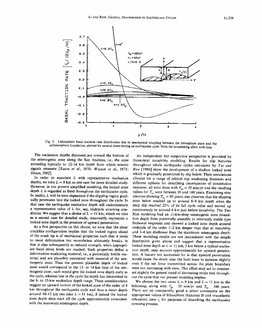
The flow in the upper mantle is transmitted to the surface plate through a mechanical coupling which produces a driving traction at the base of the lithosphere, corresponding to the i x term in (1) (after time differentiation) and is shown sche- matically in the inset in Figure 5. This basal traction varies over the earthquake cycle. Shortly after an earthquake, i x is concentrated at the base of the fault. As time progresses, the basal traction distribution broadens into the interior of the

plate. This basal traction may be calculated using (1) and (2), after the thickness averaged displacement u(y, t) has been computed from (7), and is shown in Figure 5 for various times of the earthquake cycle. The parametric values used for com- puting the basal tractions are suggested by results of the next section. It can be seen that the distribution is very broad at

11,538 LI AND RICE: CRUSTAL DEFORMATION IN EARTHQUAKE CYCLES

N

0.8

0.15

0 4

o 2

o o

L=O. 3H

T:y = 160yr tr =12yn

O O O O O O O O 4.1

CRACK FACE DISP. (Uc/Vp, tr)

Fig. 4. Displacement of shear crack wall below locked zone as a function of depth at various fractions of cycle time. Same parameters as for Figure 3b.

40% cycle time or more. An important implication of the broadness of this basal traction distribution is that the surface

deformation would also be distributed over a broad distance

from the fault trace, especially in the mid and late portion of the cycle time. Note that the surface deformation rates •i s and •;s of an elastic plate may be regarded as being determined uniquely by the basal traction rate distribution.

In calculating •i• and •.• by (12) and (13) we are effectively making an approximation in relating the basal traction rate distribution to the surface deformation rates. (The traction rates imply ri(y, t) by (1), (2) and (5), and hence •i•(y, t) by (12) and (13).) This approximation and its suitability are addressed in more detail in Appendix B. For now, we note that it is less accurate at early portions of the earthquake cycle but becomes increasingly accurate at times beyond about 40% of the earthquake cycle (Figures B1 and B2). This is associated with the broadening basal traction distribution discussed above. It also improves for locked depths less than about 50% of the plate thickness. Note that what is discussed in Appendix B is not the accuracy of our calculated traction rate distributions (Figure 5) but rather the accuracy of our simplified procedures for calculating the surface deformation rate implied by a given traction rate distribution.

The rapid asthenosphere relaxation near the base of the fault immediately after an earthquake causes a high basal traction rate there. This results in a high velocity near the fault base in comparison to the velocity farther out, say at y -- 2H, which causes a reversal in the sign of the traction rate (Figure 5) and of the associated strain rate (Figure 3) at a little more than one lithospheric thickness away from the fault trace. The strain rate reversal feature was pointed out by Lehner and Li [1982], who studied the thickness averaged deformation rates in earthquake cycles, and also shows in more exact methods of

analyzing coupling, whether to half-space or thin channel as- thenospheres [Cohen and Kramer, 1984]. This phenomenon should be measurable up to times comparable to t r after an earthquake.

MODEL PARAMETERS AND COMPARISON WITH

TIME-DEPENDENT STRAIN DATA

FROM CALIFORNIA

We wish to make our description of the earthquake loading process, which (within the framework of the model adopted) means our choice of the five parameters Vp•, L, H, Wcy and tr, consistent with seismic, geologic, and geodetic evidence from

the San Andreas fault region. Our approach is to choose Vp•, L, and Tcy on the basis of geologic and seismic considerations and then to choose the less well constrained parameters H and t, to fit the data set assembled by Thatcher [1983] for time- dependent postearthquake straining at a variety of locations along the San Andreas fault. Predictions based on the resulting parameter set are then compared to contemporary fault-parallel displacement rates as a function of distance from the fault trace at locations along the 1857 and 1906 rupture zones.

In the case of Vp• it is accepted that the overall velocity between the Pacific and North American plates is approximately 55 mm/yr [Minster and Jordan, 1978]. However, evidence from long-term fault offsets summarized recently by Minster and Jordan [1984] and Stuart [1985], based on work by $ieh and Jahns [1984] and Weldon [1984], suggests that only 35 mm/yr would be regarded as taken up by the San

Andreas fault, and we therefore set Vp• = 35 mm/yr. In northern California, great earthquakes like the 1906 rup-

ture have been estimated to have a repeat time from 70 to more than 180 years [Savage, 1983]. A longer repeat time of 225 years based on trenching data was obtained by Hall et al. [1982]. In southern California, data from extensive trenching at Pallet Creek [Sieh, 1984] lead to an average recurrence interval between 145 and 200 years for large earthquakes, based on excavated evidence of 12 earthquakes between approximately 260 and 1857 A.D. Evidence from other locations along the 1857 rupture zone [Sieh and Jahns, 1984; Stuart, 1985] suggests the possibility of a variable average recurrence interval from one segment to another, ranging from approximately 100 to 300 years. We have fixed Tcy = 160 years, since this value is reasonable in terms of observations and since

variations by _+25% (expanding the range to 120-200 years) have only modest effects on the results which we show.

In terms of the model of a locked shallow portion of the crust with accumulating aseismic slip below, it seems logically consistent that the nucleation depth for a large earthquake should be identified with the highly stressed region at the border of the slipping and locked zones, i.e., with the crack tip location. This would argue for choosing L in the range of 8-10 km on the basis of seismically determined nucleation depths. For example, the 1979 Imperial Valley earthquake is inferred to have initiated at about 8 km depth [Archuleta, 1982-1, the 1966 Parkfield earthquake at about 9 km depth [Lindh and Boore, 1981-1, and both the 1979 Coyote Lake and 1984 Morgan Hill earthquakes along the Calaveras fault at about 10 km depth [Lee, et al., 1979; Bouchon, 1982; Bakun et al., 1984]. Also Thatcher [1975] inferred a focal depth of not greater than about 10 km for the 1906 San Francisco earthquake based on analysis of geodetic data.


LLI

g

0.7

0.6

0.5

0.4

0.3

0.2

0.1

-0.0

t :-0.4To,

t-O. 6To,

t-o. 8Tcy -o. :t t-t. o'r•y

-0 o 2

To/=•60yr t• •i2yr •

-0.3 I , . i • I , J 0 ! 2 3 4

y/H

Fig. 5. Lithosphere basal traction rate distribution due to mechanical coupling between the lithosphere plate and the asthenosphere foundation, plotted for several times during an earthquake cycle. Note the broadening effect with time.

The nucleation depths discussed are toward the bottom of the seismogenic zone along the San Andreas, i.e., the zone extending typically to 12-14 km depth from which seismic signals emanate [Eaton et al., 1970; Wesson et al., 1973; Sibson, 1982].

In order to associate L with representative nucleation depths, we take L = 9 km as one case for more detailed study. However, in our present simplified modeling, the locked zone depth L is regarded as fixed throughout the earthquake cycle. In reality, L will be time-dependent if the slipping region gradually penetrates into the locked zone throughout the cycle. In that case the earthquake nucleation depth will underestimate a representative value of L for, say, midcycle straining conditions. We suggest that a choice of L = 11 km, which we take as a second case for detailed study, reasonably represents a locked zone depth in the presence of upward penetration.

As a first perspective on this choice, we note that the shear cracklike configuration implies that the locked region ahead of the crack tip is of mechanical properties such that it tends to resist deformation but nevertheless ultimately breaks, in that it slips subsequently at reduced strength, when appropriate local stress levels are reached. Such properties define a deformation-weakening material, i.e., a potentially brittle material, and are plausibly associated with material of the seismogenic zone. Thus the greatest plausible depth of locked zone would correspond to the 12- to 14-km base of the seismogenic zone; such would give the locked zone depth early in the cycle, whereas late in the cycle the depth has diminished to the 8- to 10-km nucleation depth range. These considerations suggest an upward motion of the locked zone of the order of 4

km throughout the earthquake cycle and thus a mean depth around 10-12 km (we take L = 11 km), if indeed the locked zone depth does start off the cycle approximately coincident with the maximum seismogenic depth.

An independent but supportive perspective is provided by theoretical instability modeling. Results for slip histories throughout whole earthquake cycles calculated by Tse and Rice [1986] show the development of a shallow locked zone which is gradually penetrated by slip below. Their simulations allowed for a range of critical slip weakening distances and different options for describing uncertainties of constitutive response; all were done with Vp• = 35 mm/yr and the resulting values for Ycy were between 50 and 160 years. Examining simulations showing Tcy • 80 years, one observes that the slipping zone below reached up to around 8-9 km depth when the deep slip reached 25% of its full cycle value and moved up continuously to around 6 km just before instability. The Tse- Rice modeling had an 11-km-deep seismogenic zone (transition depth from potentially unstable to inherently stable type frictional response) and showed a locked zone depth around midcycle of the order 1-2 km deeper than that at instability and 3-4 km shallower than the maximum seismogenic depth. These modeling results are not inconsistent with the simple description given above and suggest that a representative locked zone depth at L = 11 km, 2 km below a typical nucleation depth, may account approximately for upward penetration. A feature not accounted for is that upward penetration would cause the strain near the fault trace to increase slightly even if the net force transmitted across the plate boundary were not increasing with time. This effect may act to counter- act slightly the general trend of decreasing strain rate throughout the cycle that our present modeling implies.

We choose the two cases L = 9 km and L = 11 km in the

following, along with Vp• = 35 mm/yr and Ycy--160 years. There are no comparably good a priori constraints on the appropriate values of lithosphere thickness H and viscoelastic relaxation time t• for purposes of describing the earthquake stressing process.

11,540 L• AND R•CE' CRUSTAL DEFORMATION IN EARTHQUAKE CYCLES

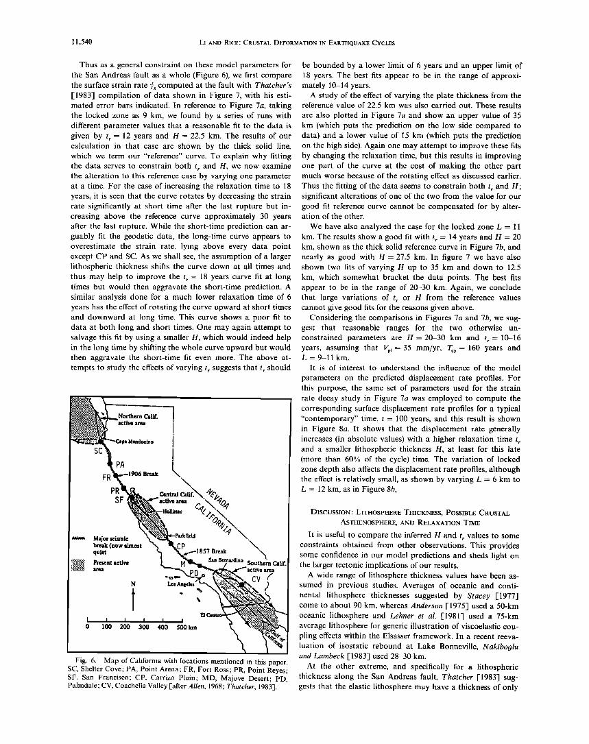
Thus as a general constraint on these model parameters for the San Andreas fault as a whole (Figure 6), we first compare the surface strain rate -• computed at the fault with Thatchef's [1983] compilation of data shown in Figure 7, with his estimated error bars indicated. In reference to Figure 7a, taking the locked zone as 9 km, we found by a series of runs with different parameter values that a reasonable fit to the data is given by t r = 12 years and H = 22.5 km. The results of our calculation in that case are shown by the thick solid line, which we term our "reference" curve. To explain why fitting the data serves to constrain both tr and H, we now examine the alteration to this reference case by varying one parameter at a time. For the case of increasing the relaxation time to 18 years, it is seen that the curve rotates by decreasing the strain rate significantly at short time after the last rupture but increasing above the reference curve approximately 30 years after the last rupture. While the short-time prediction can ar- guably fit the geodetic data, the long-time curve appears to overestimate the strain rate, lying above every data point except CP and SC. As we shall see, the assumption of a larger lithospheric thickness shifts the curve down at all times and thus may help to improve the t,- 18 years curve fit at long times but would then aggravate the short-time prediction. A similar analysis done for a much lower relaxation time of 6 years has the effect of rotating the curve upward at short times and downward at long time. This curve shows a poor fit to data at both long and short times. One may again attempt to salvage this fit by using a smaller H, which would indeed help in the long time by shifting the whole curve upward but would then aggravate the short-time fit even more. The above attempts to study the effects of varying t• suggests that t• should

Northern Calif. active ar•

Mendocino

FR 906 Break PR

SF

Major •ismic break (now almost quiet

Present active

85? Break •' San B•rn•rdino Southern Calif'.

al•a

ß t I I I I 0 !00 200 300 400 500k:m

Ell

Fig. 6. Map of California with locations mentioned in this paper. SC, Shelter Cove; PA, Point Arena; FR, Fort Ross; PR, Point Reyes; SF, San Francisco; CP, Carrizo Plain; MD, Majove Desert; PD, Palmdale; CV, Coachella Valley [after Allen, 1968; Thatcher, 1983].

be bounded by a lower limit of 6 years and an upper limit of 18 years. The best fits appear to be in the range of approximately 10-14 years.

A study of the effect of varying the plate thickness from the reference value of 22.5 km was also carried out. These results

are also plotted in Figure 7a and show an upper value of 35 km (which puts the prediction on the low side compared to data) and a lower value of 15 km (which puts the prediction on the high side). Again one may attempt to improve these fits by changing the relaxation time, but this results in improving one part of the curve at the cost of making the other part much worse because of the rotating effect as discussed earlier. Thus the fitting of the data seems to constrain both t, and H; significant alterations of one of the two from the value for our good fit reference curve cannot be compensated for by alteration of the other.

We have also analyzed the case for the locked zone L --- 11 km. The results show a good fit with tr = 14 years and H -- 20 km, shown as the thick solid reference curve in Figure 7b, and nearly as good with H--27.5 km. In figure 7 we have also shown two fits of varying H up to 35 km and down to 12.5 km, which somewhat bracket the data points. The best fits appear to be in the range of 20-30 km. Again, we conclude that large variations of t• or H from the reference values cannot give good fits for the reasons given above.

Considering the comparisons in Figures 7a and 7b, we suggest that reasonable ranges for the two otherwise un- constrained parameters are H- 20-30 km and t•= 10-16 years, assuming that Vp•--35 mm/yr, Tcy- 160 years and L = 9-11 km.

It is of interest to understand the influence of the model

parameters on the predicted displacement rate profiles. For this purpose, the same set of parameters used for the strain rate decay study in Figure 7a was employed to compute the corresponding surface displacement rate profiles for a typical "contemporary" time, t -- 100 years, and this result is shown in Figure 8a. It shows that the displacement rate generally increases (in absolute values) with a higher relaxation time t• and a smaller lithospheric thickness H, at least for this late (more than 60% of the cycle) time. The variation of locked zone depth also affects the displacement rate profiles, although the effect is relatively small, as shown by varying L = 6 km to L -- 12 km, as in Figure 8b,

DISCUSSION: LITHOSPHERE THICKNESS, POSSIBLE CRUSTAL ASTHENOSPHERE, AND RELAXATION TIME

It is useful to compare the inferred H and t• values to some constraints obtained from other observations. This provides some confidence in our model predictions and sheds light on the larger tectonic implications of our results.

A wide range of lithosphere thickness values have been assumed in previous studies. Averages of oceanic and continental lithosphere thicknesses suggested by Stacey [1977] come to about 90 km, whereas Anderson [1975] used a 50-km oceanic lithosphere and Lehner et al. [1981] used a 75-km average lithosphere for generic illustration of viscoelastic coupling effects within the Elsasser framework. In a recent reeva-

luation of isostatic rebound at Lake Bonneville, Nakiboglu and Lainbeck [1983] used 28-30 km.

At the other extreme, and specifically for a lithospheric thickness along the San Andreas fault, Thatcher [1983] suggests that the elastic lithosphere may have a thickness of only


,•, z

z

4 SAN ANDREAS FAULT, CALIFORNIA SAN ANDREAS FAULT, CALIFORNIA

T:y=160yr V½ =35mm/yr L=iikm t r -i4yp

H-20. Okra

........ H-12.5km PR

? H-27 .õkin --. -- H=35. Okra

i i I i

40 OO 220

TIME FROM LAST E.QUAKE (YRSJ TIME FROM LAST E.(•UAKE (YRS)

Fig. 7. Shear strain rate decay with time in an earthquake cycle. The data points with error bars are from Thatcher, [1983]. The solid circles are from northern California along the 1906 rupture zone of the San Andreas fault. The open circles are from southern California along the 1857 rupture zone. Curve fits are based on model with indicated parametric values.

I

16o

10 km. This was motivated by an attempt to rationalize the same data as in Figure 7, although our work here, based on what we think to be a physically more valid model, without artificial kinematic imposition of deep fault slip, shows that the data are compatible with much thicker values, 20-30 km. Further, Turcotte et al. [1984] pointed out that Thatcher's thin lithosphere would require a significantly higher heat flow than the relatively high value found over a broad region near the San Andreas fault, and they suggested a 30-km-thick three-layer lithosphere model which they coupled to the deeper surroundings by an Elsasser approximation. Their middle layer was intended to represent an intracrustal asthenosphere.

Finally, Tse et al. [1985] have modeled geodetic data from the Parkfield region and adjacent central California creeping segment of the San Andreas fault using a model similar to what we examine here, involving elastic plates locked over part of the depth range at the plate margin but freely slipping elsewhere. They assume a stress-free base for the plates and thus load the system by remotely applied forces, as in the Turcotte and Spence [1974] crack modeling, but allow the geometry of the locked ligament to vary along strike and to not exist at all within the central region of the creeping zone. They show that the fit to data is better with H in the 30-40 km range than for larger values but did not examine smaller values. Thus we can interpret their work as suggesting that H is less than approximately 40 km.

Evidently, the lithosphere thickness values of order 20-30 km that we infer are not incompatible with other studies. Further, these thicknesses are comparable to or less than representative crustal thicknesses, in that Oppenheimer and Eaton [1984] infer a Moho depth slightly above 24 km for the northern San Andreas between the PA (Point Arena) and CP (Car- rizo Plain) symbols in Figure 6, with a thickening toward 26 km within approximately 50 km of those two points and a modest thinning toward 23 km at PR (Point Reyes). The tectonic significance of this observation is that the viscoelastic asthenosphere which enters our modeling may reasonably be presumed to correspond to the lower portions of the crust and perhaps a crust-mantle transition zone.

There may, of course, also exist beneath the San Andreas fault region a classical deep asthenosphere lying beneath a more elastic layer of upper mantle material, but we tentatively conclude that it is a lower crustal asthenosphere rather than that intramantle asthenosphere which contributes to time variations in the crustal deformation rate throughout the San Andreas earthquake cycle.

An initially unexpected consequence of the inferred asthenosphere location in the lower crust is that the Elsasser-type approximation for the viscoelastic coupling becomes more suitable since the relaxation would then seem to be confined to a relatively thin channel.

The relaxation time t r is proportional to Hrl/hG, and there is considerable uncertainty associated with an a priori choice of


IT >-

E E

LLI

IT >-

E E

LLI

z w

llJ r•

._J n f•

-5

-2O

-5

-2O

, I ,. I m I m .. I , i

0 •0 20 30 40 50 6O

DISTANCE FROM FAULT [KM]

m I , i , I , .I. ,.. I ,,

iO :•0 30 40 50 6O

Fig. 8.

DISTANCE FROM FAULT [KM]

Displacement rate profiles, calculated for the parameters indicated.

a suitable asthenospheric viscosity r/ and depth scale h over which velocity gradients occur in viscous relaxation. Previous attempts to estimate r/ have generally assumed that the asthenosphere involved is of the classical intramantle type and are of uncertain relevance if a thin lower crustal asthenosphere is the correct picture. Nevertheless, with regard to r/, Nut and Mavko [1974] inferred 5 x 10 •8 Pa s from postseismic relaxation, whereas Thatcher and Rundle [1979] and Thatcher et al. [1980] suggested values of 4 x 10 •9 Pa s and 1 x 10 •9 Pa s, respectively, for postseismic lithosphere rebound at underthrust zones. Walcott [1973] inferred 5 x 10 •9 Pa s from isostatic rebound data at Lake Bonneville, and a recent reevalua-

tion of that case by Nakiboglu and Lambeck [1983] suggested r/= 1.5 to 3.4 x 10 •9 Pa s when a 28- to 30-km elastic plate is assumed to lie over a uniform viscoelastic half-space and 2.1 to 5.8 x 10 •8 Pa s when the plate lies over-a 100-km-thick channel asthenosphere.

BALD

0

Do

•NEISS

•OL•E••• • •

' ,'o '; 'LO•A •

TE• H•AC• Fig. 9. Geodetic networks in the Palmdale area [after King and

Sar, a,qe, 1984].


PALMDALE AREA

EE >.-

E E

Ld

I-- z Ld

Ld

J 0_

H

-5

T t•23yr Try= •60yr V•% =35mm/yr ...... L=• •[km H=20. Okm

,

. • , I I , I I I -'15 -:iO 0 •0 20 30 40 50

DISTANCE FROM FAULT (KM)

Fig. 10. Comparisons of theoretically predicted displacement rate profiles to geodetic data from King and Savage [1984]. Stations, in order of increasing y, are Mount Pinos, Frazier, Sawmill, Tejon 41, Tecuya, Police, Thumb, Wheeler 2, Diorite, Gneiss, and Tejon 32.

The crustal shear modulus near the San Andreas is G = 35

GPa, based on the average p wave velocity of 6.0 km/s [Op- penheimer and Eaton, 1984] and assuming a Poisson ratio of 0.25 and specific gravity of 2.9. Thus the relaxation time t r = 13 years (middle of 10- to 16-year range) implies r/= 2.3 (h/H) X 1019 Pa s. We have inferred that H = 20--30 km. Using

H = 23 km and, since the asthenosphere is assumed to be confined to the lower crust and crust-mantle transition zone, assuming that h may range from 2 to 10 km, we conclude that viscosities of 2 x 10 TM Pa s to 10 •9 Pa s are implied. These are in a range compatible with other estimates as just summarized. We have no independent check on their suitability or, indeed, on the adequacy of a linear characterization of viscoelastic response.

USE OF MODEL WITH PARAMETERS AS CHOSEN

TO PREDICT CONTEMPORARY F^ULT-P^R^LLEL

STRAIN AND DISPLACEMENT RATES

Here we compare our model predictions, based on the parameters already chosen, to data other than that used to constrain the parameters. The data consist of geodetically measured contemporary fault-parallel surface displacement rate profiles as a function of distance from the San Andreas fault, at two locations along the fault, and contemporary strain rates averaged over variable-sized areas at one of these. Within the context of a model that involves uniform conditions along strike and symmetry relative to the single fault strand representing the San Andreas in our surface plate, we believe that the comparison of prediction to data here is supportive of our model. Nevertheless, the displacement rate profiles at particular locations along strike, constructed from data for individual geodetic markers, are strongly affected by local conditions.

These suggest pronounced asymmetry of material properties or geometry relative to the San Andreas and show the effects of adjacent fault strands. Also, the data include features that suggest large nonuniformities along strike or, perhaps instead, inaccuracies relating either to marker instability relative to the crust below or to systematic measurement error. In one case, we note changes in model parameters which would improve the fit, but this is not always feasible within the symmetry of our model relative to the San Andreas fault.

Palmdale Area (Point PD in Figure 6 and Figures 9 and 10)

The displacement rate (average velocities, 1973-1983) data were deduced by King and Savage [1984] for 11 of the stations in Figure 9, from line length measurements using the "outer coordinate" solution method which minimizes the rms dis-

placement normal to the San Andreas fault. Based on the line length changes, King and Savage concluded that there was no clear evidence of surface fault slip in the Tehachapi region. This data set has a relatively large scatter and is plotted in Figure 10 with the displacement rate zeroed on the San An- dreas fault. The two theoretical curves shown are based on the

parameters of the best fits to the strain rate decay data set shown in Figures 7a and 7b. They are computed at t = 123 years (1857 + 123 = 1980), within the time period when the measurements were made. Within the scatter of data, these

parameters give apparently reasonable predictions to displacement rate profiles in the Palmdale area. The data are probably affected by the presence of the Garlock fault. King and Savage fit it with a buried screw dislocation model and conclude that

a slightly better fit is obtained if they assume deep slip on the

11,544 LI AND RICE' CRUSTAL DEFORMATION IN EARTHQUAKE CYCLES

TABLE 1. Calculated and Observed Strain Rate in the Palmdale Area

.•, (Ay) .... •3(1), •(2), 5(3), • [King and Savage, km km •tstrain/yr #strain/yr #strain/yr 1984], #strain/yr

Palmdale* -0.3 3.6 0.42 0.41 0.38 0.37 +__ 0.02 (1971-1982) SA Region* 4.1 10.4 0.37 0.38 0.33 0.34 q- 0.01 (1973-1983) Tehachapi* 17.0 20.2 0.29 0.31 0.25 0.21 + 0.01 (1973-1983) Los Padres -19.7 19.7 0.27 0.29 0.23 0.21 +__ 0.02 [McGarr

et al., 1982] Sub Garlock* 31.0 21.1 0.21 0.23 0.18 0.17 + 0.02 (1973-1983'

called Garlock region)

The • are positive to the NE. All calculations made for t = 123 years, Toy = 160 years and (1) Vv• - 35 mm/yr, L = 9 km, H -- 22.5 km, t r = 12 years' (2) Vv• = 35 mm/yr, L -- 11 km, H - 20 km, t r = 14 years' (3) Vp• = 32 mm/yr, L = 9 km, H = 25 km, tr = 12 years.

*Subdivision of Tehachapi net.

Garlock fault (at slightly less than half the rate they infer on the San Andreas), rather than slip on the San Andreas only. Their inferred locking depth is a poorly resolved 15-20 km, which we regard as somewhat questionable on seismic grounds and, in light of our results with much shallower locking depths, probably due to shortcomings of the buried dislocation model which we have discussed.

The strain rate averaged over various subnets of the network shown in Figure 9 (see Figures 5 and 6 of King and Savage [1984] for locations of the subnets) was calculated by King and Savage [1984] and is listed in Table 1. Also listed are data for the Los Padres geodetic network, lying just to the NW of the region shown in Figure 9 and mostly to the ocean side of the San Andreas [Savage, 1983], as summarized by McGarr et al. [1982]. We have calculated the corresponding strain rate from our model using the same two sets of parameters mentioned earlier. The calculation was done based on the

centroidal distance 37 of the net from the San Andreas fault (positive on continental side) and the root mean square distance (AY)rms of the stations in the net, as given by McGarr et al. [1982], and these values are also given in Table 1. The strain rate calculations were based on a procedure attributed to Savage by McGarr et al., using

•fi -- {/•s[; -3- (Ay)rms'] -- /is[• -- (AY)rms']}/2(AY)rms (15)

They implemented this formula with the buried screw dislocation model.

Our results based on our sets of reference parameters are tabulated as •(1) for the L - 9 km case and •(2) for the L - 11 km case. These calculated results are seen to be on the high side when compared to the observed strain rate. However, we have not attempted to fit this set of strain data, and the comparison can be improved by varying the model parameters. Owing to the uncertain effect of the Garlock fault, it is not clear that a fitting is justified. Nevertheless, Figures 8a and 8b show how slopes of the displacement rate profiles, i.e., the strain rates, can be altered by variation of L, H, and tr, and of course, the curves shown all have amplitude directly proportional to Vp•. We show as •(3) in Table 1 the result which corresponds to Vp• = 32 mm/yr, L = 9 km, H = 25 km, t• = 12 years, and rcy: 160 years just to emphasize that a good fit is possible with a locked depth that, we have argued, can be justified on seismological and material property considerations. In comparison, McGarr, et al. [1982] find that with the buried screw dislocation model the data imply a locked depth, again poorly constrained, around 22 km.

We may note also that the buried screw dislocation fits of King and Savage and McGarr et al. imply contemporary deep slip at rates of order 20-25 mm/yr. Our modeling shows that while points at the base of the surface plates, far removed from

the fault trace, have relative motion at rates of Vp• = 35 mm/yr, the average contemporary slip rate on the freely slipping deeper portion of our fault zone, 2[H/(H -- L)]ti(0+, t), is only of order 4.9-6.4 mm/yr. The reason for this great differ- ence will be evident from Figures 3b, 4, 5, and 8: At large times since the last earthquake the average deep slip rate di- minishes considerably, but the accommodating region of the asthenosphere broadens out to several times the plate thick- Bess.

Point Reyes Area (Point PR in Figure 6 and Figures 11 and 12)

Data for the period 1972-1982 from geodetic networks at Point Reyes (38.1øN), Santa Rosa (38.3øN), and Napa (38.0øN) were analyzed by Prescott and Yu [1986], updating data given previously by Prescott et al. [1979], These networks are shown in Figure 11. Because of the proximity in latitude of the three mentioned locations, the displacement rate values from these networks provide a profile of fault-parallel rate as a function of distance from the San Andreas. Figure 12 shows the component of surface displacement rate parallel to the fault trace, as compared to data assembled for all stations of each network by Prescott and Yu [1986]. Their displacement data are analyzed as by Prescott [1981], in that a rigid body rotation has been chosen so as to minimize displacements perpendicular to the fault trace. We have added a rigid trans- lation to the data of Prescott and Yu [1986] so that zero fault-parallel displacement occurs at the San Andreas. The triangles are from the Geyser network to the north (Figure 11).

Our theoretical curves shown in Figure 12 with these data use the same sets of best fit parameters as deduced from the strain rate decay fit (Figures 7a and 7b, heavy solid curves). That is, the parameters are chosen independently of the Point Reyes area data set. The profiles are computed at t = 73 years (1906 + 73 = 1979), within the time period when the line length measurements were made. The predicted profiles appear to match the observed displacement rates very well on the NE side of the fault up to distances well beyond the Rogers Creek fault extending to y -- 40 km. Beyond the West Napa fault, however, the data show clear deviation with higher rates than the predicted profiles. Prescott and Yu


39 øOO' KONOCTI 122o30'

BEN LOMO•// HA71N

GEYSER

WESTON

HELENA

i i i

kilom•

20

+ 125*15'

Fig. 11.

TRENTON 38o30

I TOMAS!

Point Re•s POINT

HEAD

SANTA ROSA

BURNSIDE

HOOKER

\ ! \ \\

\\ \ \\ // SLEEPY

\ ! --' "'- - ANTONiO'•x-.. -. /

//I \\ I I LL i \ /

I \

,"PT. liEYES \\ // ;ASK) • /

Son

Pablo • Bay

FARALLON

SWEENEY

RECTOR

SLAUGHT -

$/1 N .'" i'•:.

FR•NC/SCO "•!,. BAY .

,•MT. VACA / \

38ø00 122'00'

Geodetic networks in the Point Reyes-Santa Rosa-Napa area [after Prescott and Yu, 1986]

[1986] attribute these higher rates to slip on faults lying farther to the east and show that the regional distribution of seismicity is compatible with that assumption. We have assumed that the underlying mantle motion is accommodated on a single fault. It is possible to extend our modeling of whole cycle deformation in a straightforward manner to allow accommodation of the underlying mantle motion on parallel faults. Such would, however, seem to be premature for this region in view of the data now available.

While the predicted profiles in Figure 12 match the two data points close and to the SW of the San Andreas, the other data points corresponding to the Point Reyes Head and Farallon Islands station velocities show marked deviation

from an asymmetric displacement rate field about the San Andreas. We cannot judge the reliability of the data. As Pre- scott and Yu [1986] note, if valid, they suggest very much smaller shear strain rates to the SW of the fault than to the

NE and also that the shearing region which accommodates what we have called Vp] here occupies a broad zone extending to the NE of the San Andreas fault.

We have observed earlier that our relaxing asthenosphere is inferred, by fits to the strain rate decay data, to lie in the lower crust. Further, the seismically inferred crustal thicknesses by Oppenheimer and Eaton [1984] suggest that the crust is already slightly thinner near Point Reyes than elsewhere along the northern San Andreas fault and that it dimlnishes in thick-

ness at an unusually high rate as one moves toward the fault from the NE side there (approximately 1.2-km crustal thickness decrease per 10 km motion along the Earth's surface towa?d the fault there, compared to 0.6-0.8 km per 10 km elsewhere along the fault). Thus the possibility arises that the crust becomes sufficiently thin on the SW side near Point Reyes that its (now shallow) lower regions are too cool to allow much viscous relaxation. This line of argument suggests

11,546 LI AND RICE: CRUSTAL DEFORMATION IN EARTHQUAKE CYCLES

•5

LLi

i:::1 -;,5

- POTNT REYES AREA

L-gkm H-•. 5km tr-•2yr

Lm:• tkm H-20. Okm t r-tayr

NEST CORDELIA AND NAACANA NAPA GREEN VALLEY

-30 , I i m, I m I , I , I -40

DISTANCE FROM FAULT (KM)

Fig. 12. Comparisons of theoretically predicted displacement rate profiles to geodetic data from Prescott and Yu [1986], with error ranges indicated. Circles are data from Point Reyes, Santa Rosa, and Napa networks. Triangles are from Geyser network farther north. The two data points at approximately -20 km and -40 km are associated with the Point Reyes Head and Farallon Islands markers.

that the crustal asthenosphere may get pinched off to the SW side of the fault. If so, the effective lithospheric thickness would be much greater on that side. This should result in a pronounced asymmetry of surface straining relative to the fault trace, but we do not yet know how to model it to compare against the data. A further elaboration of the concept, suggested to us by R. J. O'Connell, is that the upper mantle immediately beneath such a thin crust to the SW could be too cool to deform readily and hence would move as an effectively rigid zone of material. This may be consistent with the block- like motion to the SW of the fault in Figure 12. Our discussion in this paragraph is clearly speculative and is driven by the two data points (Farallon Islands, Point Reyes Head) of uncertain significance. For example, aseisimic undersea fault regions cannot be ruled out and could influence either data point. Also, differences in crustal composition from one side of the fault to the other may be more important than differences of thickness in giving the apparent asymmetry of lower crustal relaxation.

Prescott and Yu [1986] do not attempt to model the overall physics of the driving process throughout the earthquake cycle, as here, but do provide a set of kinematical models to fit their data. Their models are based on a distribution of buried

screw dislocations in a half-space. Their preferred distribution (model E in their paper) involves spatially uniform slip at 10 mm/yr over the 6- to 10-km depth range. To this they add a rectangular zone of uniform shear strain rate, extending from 10 km to much greater depths and over the 50-km lateral distance from the San Andreas to the West Napa faults, so as to sum to 30 mm/yr total motion. In comparison, our theoretical predictions as shown in Figure 12 suggest that the observed broad deformation profile between the San Andreas and West Napa fault may result from ongoing mantle motion,

together with laterally spreading asthenospheric relaxation from the great 1906 earthquake taking place below an elastic plate of approximately 20 km depth. Our explanation is similar to that of Prescott and Yu [1986] in that both involve inelastic shear in a buried zone extending laterally from the San Andreas.

CONCLUSIONS

We have presented a physical model for the loading of an elastic surface plate near a strike-slip margin by basal shear drag, transmitted through a viscoelastic asthenosphere, from steady mantle flows. The model allows the prediction of surface strain rates and surface displacement rates near the strike- slip boundary. The major features of this model, when parameters are chosen for consistency with data from the San An- dreas fault region, are that it involves relatively thin elastic lithospheric plates (20-30 km), locked between earthquakes over shallow depths (9-11 km) at the plate margin, with continuing aseismic slip below the locked zone. The surface plates are coupled by a Maxwell viscoelastic asthenosphere, presumed to be the lower crust and perhaps a crust-mantle transition zone of viscosity r/= 2 x 10 •8 to 10 •9 Pa s, to upper mantle motions compatible with overall plate motions. The surface deformation is shown to be localized to the plate boundary (to within approximately three lithospheric plate thicknesses) due to deep aseismic slip below a locked brittle upper crust, modeled as stable shear sliding of crack faces at constant resistive stress in the antiplane strain deformation of an edge cracked elastic strip.

The viscoelastic coupling is treated approximately by a generalized Elsasser model which provides the time dependence of plate loading as well as the time dependence of the surface displacement and strain rates following sudden slips of the

Li AND RICE' CRUSTAL DEFORMATION IN EARTHQUAKE CYCLES 11,547

locked zoneß Thus the complete earthquake cycle is modeled as sudden slip on the shallow locked upper crust (partially penetrating the aseismic shear zone) during an earthquake, which loads the asthenosphere. This is followed by the relaxation of the asthenosphere which reloads the surface plate, and this loading causes continuing aseismic slip below the now locked zone. Because of the relaxation effect of the as-

thenosphere, the stress accumulation and the surface deformation rates are nonlinear in time over the earthquake cycle.

An additional effect of the relaxation is that while the San

Andreas fault may accommodate an overall slip rate of 35 mm/yr, the contemporary slip rate below the locked zone may be much smaller than 35 mm/yr. We estimate that it is cur- rently about 5 mm/yr beneath the locked 1857 rupture zone. The substantially higher slip rate shortly after an earthquake rupture makes up the deficiency and produces an average rate of 35 mm/yr over the earthquake cycle.

The present model has five parameters, with the plate velocity, locked fault depth, and the earthquake recurrence interval chosen from seismic and geologic evidence. The remaining two parameters, the lithosphere plate thickness and the asthenosphere relaxation time, are constrained by the composite time decay strain rate data [Thatcher, 1983] for the San Andreas fault. The resulting parameter set was then applied to predict the contemporary surface deformation rate profiles at Point Reyes and Palmdale, providing acceptable fits.

The simple single-fault geometry as contained in the present version of the model cannot account for data affected by motions on branch faults or by material properties which are not distributed symmetrically about the San Andreas. The model presented here has other limitations. For example, the aseismic shear zone at depth is assumed to creep slip under constant resistive stress. However, in reality it may be expected that this zone supports larger stresses just after the earthquake in the shallow crust and then relaxes with time, producing a second, presumably short-term, source of time dependence. Also, there are simplifying approximations inherent in our use of the Elsasser foundation concept and Turcotte-Spence edge cracked strip solution which could be improved upon in future work.

APPENDIX A: SOLUTION OF DIFFERENTIAL EQUATION

We reproduce here the governing equation (4):

(0• q- flC3/c3t)c32U/C3y 2 = 63U/C3t (A1)

for the part of u that must respond to the first periodic sawtooth term in (6). This part is subject to the boundary condition (5) with D given by the sawtooth. We introduce the normalized parameters

y • y/ill/2 T = •t/fi = tit r (A2)

2 = G/2kfi 1/2 = (8/rr 2) In [1/sin (•L/2H)]

We first look for the solution to the fundamental problem of a periodic slip function D = Do ei•øt and later superimpose all frequencies co to form the complete solution to our problem. Let u(Y, T) = uo(Y)e i•øt. Then it may be shown that

uo(Y ) = [Do/2B(co) ] exp {--M(co)Y

-iEN(co)Y + tp(co)]} (A3) where

M(co) = {co[p(co) + co]/2[p(co)] 2} 1/2 (A4a)

N(co) = {co[p(co) -- co]/2[p(co)] 2} 1/2 (A4b)

p(o•) = (1 + o•) •/•

B(co) = [1 + 22M(co) + 22co/p(co)] 1/2

tp(co) = arctan {2N(co)/[1 + 2M(co)] }

Hence for D(T) = Im (Do ei•T) = D O sin coT,

u(Y, T) = [D O/2B(co)] exp [ -- M(co) Y]

(A4c)

(A4d)

(A4e)

ß sin [co T -- N(co) Y -- ½(co)] (AS)

As the periodic sawtooth function may be represented by an infinite sine series, the solution for u(Y, T) also takes the form of a sine series, made up of fundamental solutions given by (A8) with the appropriate frequency co. The complete form of u(Y, T) is given by equation (7). For numerical convergence, we have removed terms summing to known discontinuous functions of time (e.g., sawtooths) from within the summation signs. The actual expression used for numerical computation is given below for the thickness averaged displacement rate:

' 63l• (Y, t)= ' e-Y [•(• •ycy)( )• Vpl3t •+1+2 -- 1+2 +Y •-- tr

where

sin (cont/tr) + fl. COS (cont/tr) ] (A6)

e-•U"r e-r (2__••)()- ) y. - sin (½% + YN.)- + Y (A7a) B. 1 +2 1 +2

e -MnY e- Y fl,- cos (½, + YN,)- • (A7b)

B, 1+2

co. = 2rcntr/Tcy (A7c)

and where M,, N,, p,, B,, and ½, are the functions of co given above evaluated at co = co,. Also, for the thickness averaged shear strain rate, we use

H 632u 2 e-¾ [ 1 (ycy•( 1 - 1+ Y - Vpl •y•t rc 1 +2 • \ t• ?\ l +2

-f•r•2[(1/6) - (t/Toy) 4- (t/Tcy) 23

- y. [0. sin (co.t/t•) + 7. cos (co.t/tO] (A8)

where

3 + 2 I (A9a) (1• 2 4

0, = --- e-•t"r[N, cos (½, + N,Y) -- M, sin (½, + N,Y)] rob n

+ i½} '1+2 Y (A9b) •con

4 [e- MnY 7, =- [M, cos (½, + N,Y) rc B n

+ N, sin (½, + N,Y)] -- (A9c) 1 + rr 2

Notice that all the coefficients or,, fl,, 0, and 7, of the sine and cosine terms in the summations vanish as 1In 2 as n--• •, which accelerates the series convergence. Equations (A6) and (A8) are the actual expressions used for numerical evaluation of equations (12) and (13).

11,548 Li AND RICE: CRUSTAL DEFORMATION IN EARTHQUAKE CYCLES

w i- <( n-

F-

LLI

W

<( _J CL

•J

O.B _

0.15

0.4

0.2

0.0

L=O. 33H a

t =0.2 T• .-• .23

EXACT

......... APPROX.

i I i i

o ! 2 3 4 5

0.6

o 4

o 2

o o

L=O. 5H

L=O . 2Toy

EXACT

......... APPROX.

LU

z LLJ

W

_J CL

Ld

LL

DISTANCE FROM FAULT TRACE

0.8 _ L=O. 33H

0.6

0,4

0.2

0.0

t =0 . 5 Tcy

EXACT

......... APPROX ß

(y/H)

O.B _

DISTANCE FROM FAULT TRACE (y/H)

o.15

L=O . 5H

0.4

O.E

I 0.0

t=O . 5T c¾

EXACT

......... APPROX.

/ /

/ /

0 •. E 3 4 5 0 :1 2 3 4 5

DISTANCE FROM FAULT TRACE (y/H) DISTANCE FROM FAULT TRACE

Fig. B1. Comparison of prediction of surface displacement rate for two cycle times and for two locked depths, based on an approximate method (dotted curves) used in the text, and an "exact" method (solid curves) described in Appendix B.

(y/H)

APPENDIX B' COMPARISON OF SURFACE DISPLACEMENT

ESTIMATION BY EQUATIONS (12) AND (13) WITH THAT BY AN "EXACT" METHOD

Equations (12) and (13) involve approximations in estimation of surface displacement from the thickness averaged

quantities. The formulation is exact when the load is applied directly on the lateral surfaces of the lithospheric plates, as in Figure lb. However, our model involves coupling and hence shear traction transfer between the lithosphere and asthenosphere, i.e., the surface deformation rates depend on the lithosphere basal traction rate distribution (Figure 5).

LI AND RICE: CRUSTAL DEFORMATION IN EARTHQUAKE CYCLES 11,549

1 2

i 0

0 8

0 6

0 4

0 2

C 0

-0.2

F L=O. 33H a

t = 0 . 2. Tc,,/

EXACT

......... APPROX.

! I i f i i ! ! i J

0 •. 2 3 4 5

h- <•

Z

1 2

I o

o 6

o 4

o 2

o o

-0.2

L=O .SH

L =0 . 2Tc¾

EXACT

......... APPROX.

o :t 2 3 4

LU

Z

o 5

o 4

o 3

o 2

o I

o o

DIS-rANCE FROM FAULT TRACE (y/H)

L=O. 33H

t =0 . 5Tcy

EXACT

......... APPROX. LU

Z H 0.2_

<• o.l

DISTANCE FROM FAULT TRACE (y/H)

0,5 _

0.0

L=O . 5H

t =0,5Toy

EXACT

......... APPROX.

0 I 2 3 4 5 o I 2 3 4 5

DISTANCE FROM FAULT TRACE (y/H) DTSTANCE FROM FAULT TRACE

Fig. B2. Comparison of prediction of surface strain rate for two cycle times and for two locked depths, based on an approximate method (dotted curves) used in the text, and an "exact" method (solid curves) described in Appendix B.

(y/H)

The approximate method of estimating fis in terms of i x adopted in the paper involves equations (1), (2), (5), (12), and (13). It is equivalent to writing (when D(t) = O)

ds(y ) = [dxy(O)/2k]S(y ) + [dx•,(y)/G ] dy (B1)

where

This step can also be done exactly, and we do so in this appendix. The exact method makes use of a Green's function

11,$$0 Li AND RICE' CRUSTAL DEFORMATION IN EARTHQUAKE CYCLES

derived for a pair of symmetrically located line loads acting on the base of the lithosphere with opposite sense (see inset in Figure 5 for the geometry). This Green's function is then used in a superposition scheme to sum up the effect of a continuous distribution of basal tractions as given in Figure 5, and the summation can be written as

tit(y ) = G(y, Y')'•x(Y') dy' (B3)

for calculation of the surface displacement rate. In (B3), tx(Y') dy' represents the infinitesimal line load magnitude at y' and ?x(Y') is of course the basal traction rate at y' shown sche- matically in the inset of Figure 5. The Green's function G(y, y') has been derived IV. C. Li and H. S. Lim, unpublished manuscript, 1987] using analytic function theory and conformal mapping techniques, and is given by

1 Re log (B4)

where z = y + iz and f•(k) = [1 + tanh 2 (•rk/2H)/ tan2(•ra/2H)] •/2. Naturally, the corresponding Green's function for surface strain rate can be obtained by direct differentiation of (B4).

Results for the predicted surface displacement and strain

rates are compared for two cycle times (one early, t = 0.2rcy and one mid cycle, t = 0.5Toy ) and for two locked depths, as shown in Figures B1 and B2. The curves labeled "exact" (solid) are based on the Green's function method just described, whereas the ones labeled "approx." (dotted) are based on the method used in the main text of this paper. They show that the approximate solution approaches that of the exact calculation at mid and late cycle times and for adequately shallow locked depths. For the surface displacement rate, the inaccuracy at early times (Figures B la and B lb) occurs at a distance of one lithosphere thickness from the fault trace and beyond. It may be noted that the predicted surface strain rate at Palmdale tabulated in Table 1 and surface displacement rates profiles predicted at Palmdale and Point Reyes in Fig- ures 10 and 12 are computed at mid and late cycle times, so that confidence may be placed on the appropriateness of the use of the approximate method.

Acknowledgments. The authors wish to thank H. S. Lim for making computational runs in the preparation of this manuscript and to acknowledge comments on earlier versions of this manuscript by N. E. King, R. Stein, W. Thatcher, and unidentified reviewers which contributed to the improvement of the paper. The manuscript has been typed by M. Weir. V.C.L. was supported at the start of this work by grants from the National Science Foundation, and U.S. Geological Survey, to the Massachusetts Institute of Technology (MIT) and, for the completion of the work, by a NASA grant to MIT; J.R.R. was supported throughout by NSF and USGS grants to Harvard.

REFERENCES

Allen, C. R., The tectonic environments of seismically active and inac- tive areas along the San Andreas fault system, Proceedings, Confer- ence on Geological Problems of San Andreas Fault System, edited by W. R. Dickinson and A. Grantz, Stanford Unit,. Publ. Geol. Sci., 11, 70-82, 1968.

Anderson, D. L., Accelerated plate tectonics, Science, 187, 1077-1079, 1975.

Archuleta, R. J., Hypocenter for the 1979 Imperial Valley Earthquake, Geophys. Res. Lett., 9, 625-628, 1982.

Bakun, W. H., M. M. Clark, R. S. Cockerham, W. L. Ellsworth, A. G.

Lindh, W. H. Prescott, A. F. Shakal, and P. Spudich, The 1984 Morgan Hill California earthquake, Science, 225, 288-291, 1984.

Bouchon. M., The rupture mechanism of the Coyote Lake earthquake of August 6, 1979 inferred from near field data, Bull. Seismol. Soc. Am., 72, 745-758, 1982.

Carlson, R., H. Kanamori, and K. McNally, A survey of microearth- quake activity along the San Andreas fault from Carrizo Plain to Lake Hughes, Bull. Seismol. Soc., 69, 177-186, 1979.

Cohen, S.C., and M. J. Kramer, Crustal deformation, the earthquake cycle, and model of viscoelastic flow in the asthenosphere, Geophys. d. R. Astron. Soc., 78, 735-750, 1984.

Eaton, J.P., M. E. O'Neill, and J. N. Murdock, Aftershocks of the 1966 Parkfield-Cholame, California earthquake: A detailed study, Bull. Seismol. Soc. Am., 60, 1151-1197, 1970.

Hall, N. T., E. A. Nelson, and D. R. Fowler, Holocene activity on the San Andreas fault between Crystal Springs Reservoir and San An- dreas Dam, San Mateo Country, Calif., paper presented at 78th, Annual Meeting, Cordilleron Sect., Geol. Soc. of Am., Anaheim, Calif., 1982.

King, N. E., and J. C. Savage, Regional deformation near Palmdale, California, 1973-1983, d. Geophys. Res., 89, 2471-2477, 1984.

Lee, W. H. K., D. G. Herd, V. Cognetti, W. H. Bakun, and A. Raport, A preliminary study of the Coyote Lake earthquake of August 6, 1979 and its major aftershocks, U.S. Geol. Surv. Open File Rep., 79-1621, 1979.

Lehner, F. K., V. C. Li, and J. R. Rice, Stress diffusion along rupturing plate boundaries, d. Geophys. Res., 86, 6155-6169, 1981.

Lehner, F. K., and V. C. Li, Large-scale characteristics of plate boundary deformations related to the post-seismic readjustment of a thin asthenosphere, Geophys. d. R. Astron. Sot., 71, 775-792, 1982.

Lindh, A. G., and D. M. Boore, Control of rupture by fault geometry during the 1966 Park field earthquake, Bull. Seismol. Soc. Am., 71, 95 116, 1981.

McGarr, A., M.D. Zoback, and T. C. Hanks, Implications of an elastic analysis of in-situ stress measurements near the San Andreas fault, d. Geophys. Res., 87, 7797-7896, 1982.

Meissner, R., and J. Strehlau, Limits of stress in continental crusts and their relation to the depth-frequency distribution of shallow earthquakes, Tectonics, 1, 73-89, 1982.

Minster, J. B., and T. H. Jordan, Present-day plate motions, J. Geo- phys. Res., 83, 5531-5554, 1978.

Minster, J. B., and T. H. Jordan, Vector constraints on quanternary deformation of the western United States east and west of the San

Andreas fault, in Tectonics and Sedimentation Along the California Margin, edited by J. K. Crouch and S. B. Bachman, pp. 1-16, Pacific Section, Society of Economic Paleontologists and Mineral- ogists, San Diego, Calif., 1984.

Nakiboglu, S. M. and K. Lambeck, A reevaluation of the isostatic rebound of Lake Bonneville, d. Geophys. Res., 88, 10,439-10,448, 1983.

Nur, A., and G. Mavko, Post-seismic viscoelastic rebound, Science, 183, 204-206, 1974,

Oppenheimer, D. H., and J.P. Eaton, Moho orientation beneath central California from earthquake travel time, J. Geophys. Res., 89, 10,267-10,282, 1984.

Prescott, W. H., The determination of displacement fields from geodetic data along a strike slip fault, J. Geophys. Res., 86, 6067-6072, 1981.

Prescott, W. H., and S. B. Yu, Geodetic measurement of horizontal deformation in the northern San Francisco Bay region, California, d. Geophys. Res., 91, 7475-7484, 1986.

Prescott, W. H., J. C. Savage, and W. T. Kinoshita, Strain accumulation rates in the western United States between 1970 and 1978, J. Geophys. Res., 84, 5423-5435, 1979.

Rice, J. R., The Mechanics of earthquake rupture, in Physics of the Earth's Interior, edited by A.M. Dziewonski and E. Boschi, pp. 555-649, Italian Physical Society/North Holland, Amsterdam, 1980.

Savage, J. C., Strain accumuation in western United States, Annu. Rev. Earth Planet. Sci., 11, 11-43, 1983.

Savage, J. C., and R. O. Burford, Geodetic determination of relative plate motion in central California, J. Geophys., Res., 78, 832-845, 1973.

Savage, J. C., and W. H. Prescott, Asthenosphere readjustment and the earthquake cycle, J. Geophys. Res., 83, 3369-3376, 1978.

Sibson, R. H., Fault zone models, heat flow, and the depth distribution of earthquakes in the continental crust of the United States, Bull. Seismol. Soc. Am., 72, 151-163, 1982.

LI AND RICE: CRUSTAL DEFORMATION IN EARTHQUAKE CYCLES 11,551

Sieh, K. E., Lateral offsets and revised dates of large prehistoric earthquakes at Pallet Creek, southern California, J. Geophys. Res., 89, 7641-7670, 1984.

Sieh, K. E., and R. H. Jahns, Holocene activity of the San Andreas fault at Wallace Creek, California, Geol. Soc. Am. Bull., 95, 883-896, 1984.

Stacey, F. D., Physics of the Earth, 2nd ed., John Wiley, New York, 1977.

Stuart, W. D., Instability model for recurring large and great earthquakes in southern California, Pure Appl. Geophys., 122, 793-811, 1985.

Tada, H., P. C. Paris, and G. R. Irwin, The Stress Analysis of Cracks Handbook, Del Research Corporation, Hellertown, Pa., 1973.

Thatcher, W., Strain accumulation and release mechanism of the 1906 San Francisco earthquake, J. Geophys. Res., 80, 4862-4872, 1975.

Thatcher, W., Nonlinear strain build-up and the earthquake cycle on the San Andreas fault, J. Geophys. Res., 88, 5893-5902, 1983.

Thatcher, W., and T n •,,,•l•, A ,•,•1 r,•,- the earthq,,•k• c. yc•1o in underthrust zones, J, Geophys. Res., 84, 5540-5556, 1979.

Thatcher, W., T. Matsuda, T. Kato, and J. B. Rundle, Lithospheric loading by the 1896 Riku-u earthquake, northern Japan: Impli- cations for plate flexure and asthenospheric rheology, J. Geophys. Res., 85, 6429-6439, 1980.

Tse, S. T., and J. R., Rice, Crustal earthquake instability in relation to the depth variation of frictional slip properties, J. Geophys. Res., 91, 9452-9472, 1986.

Tse, S. T., R. Dmowska, and J. R. Rice, Stressing of locked patches along a creeping fault, Bull. Seismol. $oc. Am., 75, 709-736, 1985.

Turcotte, D. L., and D. A. Spence, An analysis of strain accumulation on a strike-slip fault, J, Geophys. Res., 79, 4407-4412, 1974.

Turcotte, D. L., J. Y. Liu, and F. H. Kulhawy, The role of an intracrustal asthenosphere on the behavior of major strike-slip faults, J, Geophys. Res., 89, 5801-5816, 1984.

Walcott, R. I., Structure of the earth from glacio-isostatic rebound, Annu. Rev. Earth Planet. Sci., 1, 15-37, 1973.

Weldon, R. J., Implications of the age and distribution of the late Cenozoic stratigraphy in Cajon Pass, southern California, in San Andreas Fault-Cajon Pass to Wrightwood, Guideb. 55, edited by R. L. Hester and D. E. Halliger, pp. 9-16, Pacific Section, American Association of Petroleum Geologists, Los Angeles, Calif., 1984.

Wesson, R. L., R. O. Burford, and W. L. Ellsworth, Relationship between seismicity, fault creep, and crustal loading along the central San Andreas fault, Proceedings of Conference on Tectonic Problems of the San Andreas Fault System, edited by R. L. Kovach and A. Nur, Stanford Univ. Publ. Geol. Sci., 13, 303-321, 1973.

V. C. Li, Department of Civil Engineering, Massachusetts Institute of Technology, Cambridge, MA 02139.

J. R. Rice, Division of Applied Science, Harvard University, Cam- bridge, MA 02138.

(Received November 1, 1986; revised June 19, 1987;

accepted May 29, 1987.)

crustal deformation in great california earthquake...

Documents