Crystal Structure

1

3.1 Some Basic Concepts of Crystal Structure: Basis and Lattice A crystal lattice can always be constructed by the repetition of a fundamental set of translational vectors in real space a, b, and c, i.e., any point in the lattice can be written as:

r = n1a + n2b + n3c. (3.1) Such a lattice is called a Bravais lattice. The translational vectors, a, b, and c are the primitive vectors. Note that the choice for the set of primitive vectors for any given Bravais lattice is not unique.

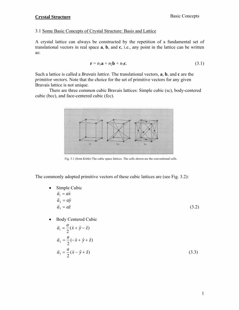
There are three common cubic Bravais lattices: Simple cubic (sc), body-centered cubic (bcc), and face-centered cubic (fcc).

The commonly adopted primitive vectors of these cubic lattices are (see Fig. 3.2):

Simple Cubic xaa

1

yaa ˆ2

zaa ˆ3

(3.2)

Body Centered Cubic

)ˆˆ(21 zyxa

a

)ˆˆ(22 zyxa

a

)ˆˆ(23 zyxa

a (3.3)

Fig. 3.1 (from Kittle) The cubic space lattices. The cells shown are the conventional cells.

Basic Concepts

Crystal Structure

2

Face Centered Cubic

)ˆ(1 yxaa

)ˆˆ(2 zyaa

)ˆ(3 zxaa (3.4)

Fig. 3.2

Coordination number: The points in a Bravais lattice that are closest to a given point are called its nearest neighbors. Because of the periodic nature of a Bravais lattice, each point has the same number of nearest neighbors. This number is called the coordination number. For example, a sc lattice has coordination number 6; a bcc lattice, 8; a fcc lattice, 12. Primitive unit cell: A volume in space, when translated through all the lattice vectors in a Bravais lattice, fills the entire space without voids or overlapping itself, is a primitive unit cell (see Figs. 3.3 and 3.4). Like primitive vectors, the choice of primitive unit cell is not unique (Fig. 3.3). It can be shown that each primitive unit cell contains precisely one lattice point unless it is so chosen that there are lattice points lying on its surface. It then follows that the volume of all primitive cells of a given Bravais lattice is the same.

(a) (b)

Basic Concepts

Crystal Structure

3

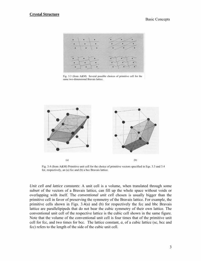
Unit cell and lattice constants: A unit cell is a volume, when translated through some subset of the vectors of a Bravais lattice, can fill up the whole space without voids or overlapping with itself. The conventional unit cell chosen is usually bigger than the primitive cell in favor of preserving the symmetry of the Bravais lattice. For example, the primitive cells shown in Figs. 3.4(a) and (b) for respectively the fcc and bbc Bravais lattice are parallelipipeds that do not bear the cubic symmetry of their own lattice. The conventional unit cell of the respective lattice is the cubic cell shown in the same figure. Note that the volume of the conventional unit cell is four times that of the primitive unit cell for fcc, and two times for bcc. The lattice constant, a, of a cubic lattice (sc, bcc and fcc) refers to the length of the side of the cubic unit cell.

Fig. 3.3 (from A&M) Several possible choices of primitive cell for the same two-dimensional Bravais lattice.

Fig. 3.4 (from A&M) Primitive unit cell for the choice of primitive vectors specified in Eqs. 3.3 and 3.4 for, respectively, an (a) fcc and (b) a bcc Bravais lattice.

(a) (b)

Basic Concepts

Crystal Structure

4

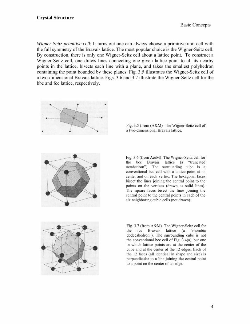
Wigner-Seitz primitive cell: It turns out one can always choose a primitive unit cell with the full symmetry of the Bravais lattice. The most popular choice is the Wigner-Seitz cell. By construction, there is only one Wigner-Seitz cell about a lattice point. To construct a Wigner-Seitz cell, one draws lines connecting one given lattice point to all its nearby points in the lattice, bisects each line with a plane, and takes the smallest polyhedron containing the point bounded by these planes. Fig. 3.5 illustrates the Wigner-Seitz cell of a two-dimensional Bravais lattice. Figs. 3.6 and 3.7 illustrate the Wigner-Seitz cell for the bbc and fcc lattice, respectively.

Fig. 3.5 (from (A&M) The Wigner-Seitz cell of a two-dimensional Bravais lattice.

Fig. 3.6 (from A&M) The Wigner-Seitz cell for the bcc Bravais lattice (a “truncated octahedron”). The surrounding cube is a conventional bcc cell with a lattice point at its center and on each vertex. The hexagonal faces bisect the lines joining the central point to the points on the vertices (drawn as solid lines). The square faces bisect the lines joining the central point to the central points in each of the six neighboring cubic cells (not drawn).

Fig. 3.7 (from A&M) The Wigner-Seitz cell for the fcc Bravais lattice (a “rhombic dodecahedron”). The surrounding cube is not the conventional bcc cell of Fig. 3.4(a), but one in which lattice points are at the center of the cube and at the center of the 12 edges. Each of the 12 faces (all identical in shape and size) is perpendicular to a line joining the central point to a point on the center of an edge.

Basic Concepts

Crystal Structure

5

Crystal Structure In the above, we have discussed the concept of crystal lattice. To complete a crystal structure, one needs to attach the basis (a fixed group of atoms) to each lattice point, i.e.,

Bravais Lattice + Basis = Crystal Structure

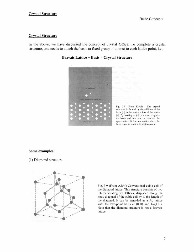
Some examples: (1) Diamond structure

Fig. 3.8 (From Kittel) The crystal structure is formed by the addition of the basis (b) to the lattice points of the lattice (a). By looking at (c), you can recognize the basis and then you can abstract the space lattice. It does not matter where the basis is put in relation to a lattice point.

Fig. 3.9 (From A&M) Conventional cubic cell of the diamond lattice. This structure consists of two interpenetrating fcc lattices, displaced along the body diagonal of the cubic cell by ¼ the length of the diagonal. It can be regarded as a fcc lattice with the two-point basis at (000) and 1/4(111). Note that the diamond structure is not a Bravais lattice.

Basic Concepts

Crystal Structure

6

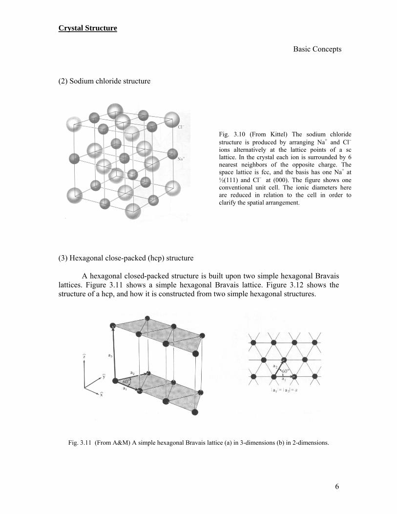
(2) Sodium chloride structure

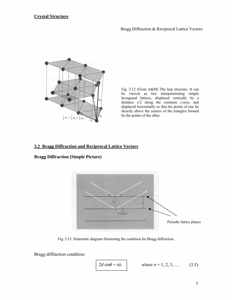
(3) Hexagonal close-packed (hcp) structure

A hexagonal closed-packed structure is built upon two simple hexagonal Bravais lattices. Figure 3.11 shows a simple hexagonal Bravais lattice. Figure 3.12 shows the structure of a hcp, and how it is constructed from two simple hexagonal structures.

Fig. 3.11 (From A&M) A simple hexagonal Bravais lattice (a) in 3-dimensions (b) in 2-dimensions.

Fig. 3.10 (From Kittel) The sodium chloride structure is produced by arranging Na+ and Cl

ions alternatively at the lattice points of a sc lattice. In the crystal each ion is surrounded by 6 nearest neighbors of the opposite charge. The space lattice is fcc, and the basis has one Na+ at ½(111) and Cl at (000). The figure shows one conventional unit cell. The ionic diameters here are reduced in relation to the cell in order to clarify the spatial arrangement.

Basic Concepts

Crystal Structure

7

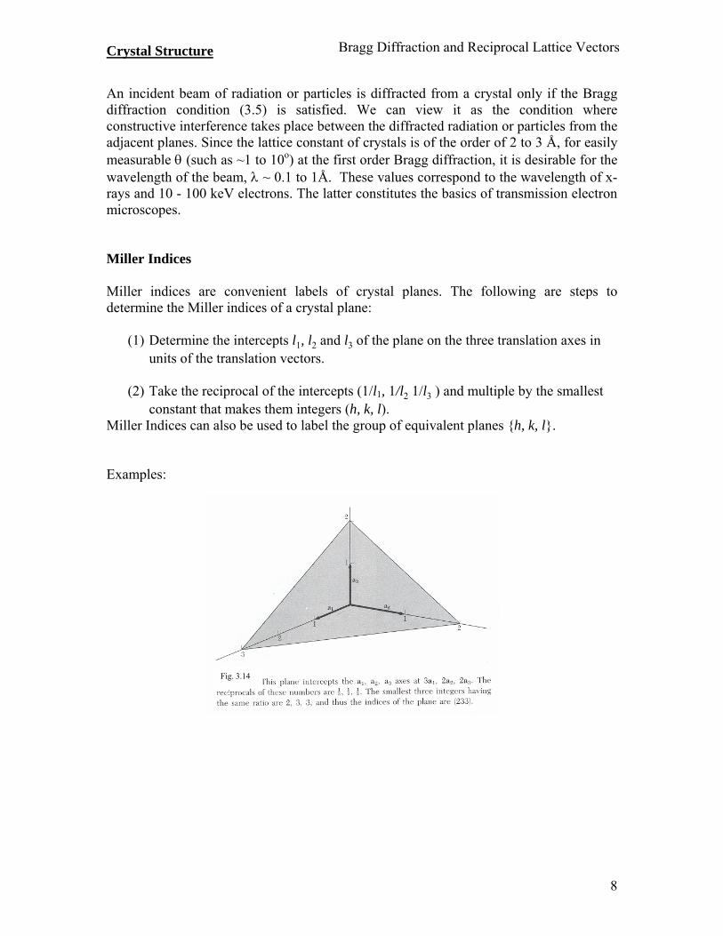
3.2 Bragg Diffraction and Reciprocal Lattice Vectors Bragg Diffraction (Simple Picture)

Fig. 3.13 Schematic diagram illustrating the condition for Bragg diffraction.

Bragg diffraction condition:

where n = 1, 2, 3, … (3.5)

Bragg Diffraction & Reciprocal Lattice Vectors

Fig. 3.12 (From A&M) The hcp structure. It can be viewed as two interpenetrating simple hexagonal lattices, displaced vertically by a distance c/2 along the common c-axis, and displaced horizontally so that the points of one lie directly above the centers of the triangles formed by the points of the other.

2d sin = n

Periodic lattice planes

Crystal Structure

8

An incident beam of radiation or particles is diffracted from a crystal only if the Bragg diffraction condition (3.5) is satisfied. We can view it as the condition where constructive interference takes place between the diffracted radiation or particles from the adjacent planes. Since the lattice constant of crystals is of the order of 2 to 3 Å, for easily measurable (such as ~1 to 10o) at the first order Bragg diffraction, it is desirable for the wavelength of the beam, ~ 0.1 to 1Å. These values correspond to the wavelength of x-rays and 10 - 100 keV electrons. The latter constitutes the basics of transmission electron microscopes. Miller Indices Miller indices are convenient labels of crystal planes. The following are steps to determine the Miller indices of a crystal plane:

(1) Determine the intercepts l1, l2 and l3 of the plane on the three translation axes in units of the translation vectors.

(2) Take the reciprocal of the intercepts (1/l1, 1/l2 1/l3 ) and multiple by the smallest

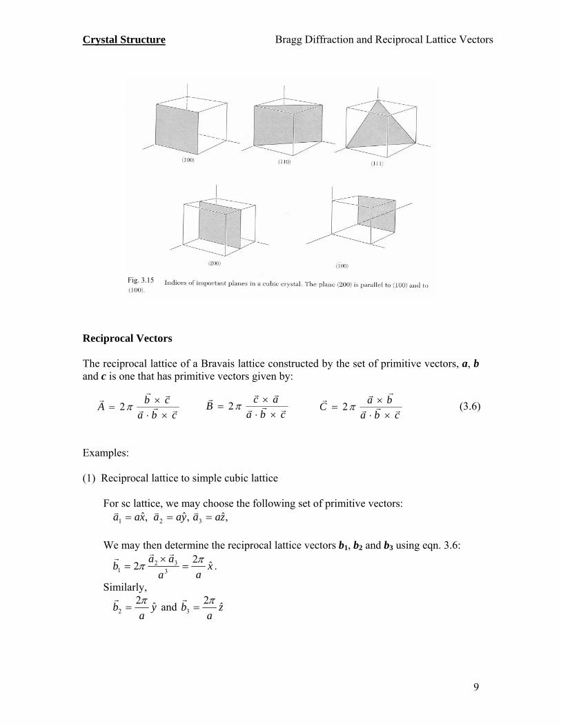
constant that makes them integers (h, k, l). Miller Indices can also be used to label the group of equivalent planes {h, k, l}. Examples:

(2, 3, 3)

Fig. 3.14

Bragg Diffraction and Reciprocal Lattice Vectors

Crystal Structure

9

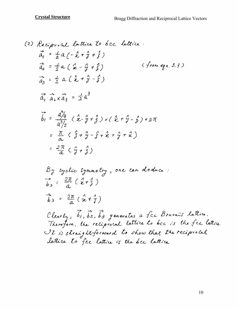
Reciprocal Vectors The reciprocal lattice of a Bravais lattice constructed by the set of primitive vectors, a, b and c is one that has primitive vectors given by:

Examples: (1) Reciprocal lattice to simple cubic lattice

For sc lattice, we may choose the following set of primitive vectors: ,ˆ1 xaa ,ˆ2 yaa

,ˆ3 zaa

We may then determine the reciprocal lattice vectors b1, b2 and b3 using eqn. 3.6:

xaa

aab ˆ

22

332

1

.

Similarly,

ya

b ˆ2

2

and z

ab ˆ

23

Fig. 3.15

Ab c

a b c

2

Bc a

a b c

2

Ca b

a b c

2 (3.6)

Bragg Diffraction and Reciprocal Lattice Vectors

Crystal Structure

10

Bragg Diffraction and Reciprocal Lattice Vectors

Crystal Structure

11

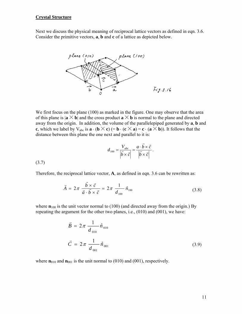
Next we discuss the physical meaning of reciprocal lattice vectors as defined in eqn. 3.6. Consider the primitive vectors, a, b and c of a lattice as depicted below.

We first focus on the plane (100) as marked in the figure. One may observe that the area of this plane is |a b| and the cross product a b is normal to the plane and directed away from the origin. In addition, the volume of the parallelepiped generated by a, b and c, which we label by Vabc is a (b c) (= b (c a) = c (a b)). It follows that the distance between this plane the one next and parallel to it is:

cb

cba

cb

Vd abc

100 .

(3.7) Therefore, the reciprocal lattice vector, A, as defined in eqn. 3.6 can be rewritten as: (3.8) where n100 is the unit vector normal to (100) (and directed away from the origin.) By repeating the argument for the other two planes, i.e., (010) and (001), we have: (3.9) where n010 and n001 is the unit normal to (010) and (001), respectively.

100100

ˆ1

22 ndcba

cbA

010010

ˆ1

2 nd

B

001001

ˆ1

2 nd

C

Crystal Structure

12

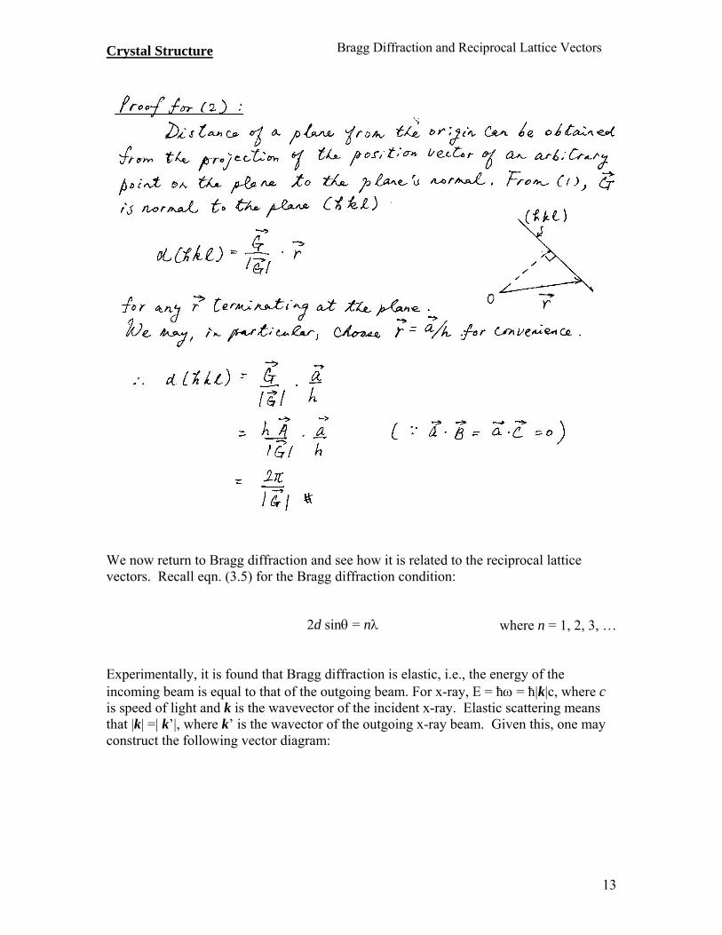
The above result can be generalized to an arbitrary reciprocal lattice vector, G = hA + kB + lC. In other words, G is related to the plane (h k l) by the following relations:

(1) G is normal to the plane (h k l). (2) The distance dhkl between adjacent planes with the Miller indexes (h k l) is given

by 2/|G|. Proof: (1) By definition, a plane (h k l) intersects the crystallographic axes along a, b and c at the points l1a, l2b and l3c, respectively, where

lkhlll

1:

1:

1:: 321

where l1, l2 and l3 are integers. Now, all planes whose intercepts fulfill the above relation are parallel. Therefore, it suffices to prove that the one plane with intercepts 1/h, 1/k and 1/l is perpendicular to G. One may observe that any vector on this plane can be expressed as a linear combination of the vectors (1/h)a – (1/k)b, (1/k)b – (1/l)c and (1/l)c – (1/h)a. It follows that if G is perpendicular to all of these three vectors, G must be parallel to (h k l). As shown below, this is indeed the case.

Note that this proof works only if none of h, k or l is zero. Suppose l = 0. Then the plane to be considered is spanned by (1/h)a – (1/k)b and c. It is straightforward to show that hA + kB is perpendicular to these two vectors. In the case where two of the Miller indices are zero, say k = l = 0, G = A. We have shown above that it is perpendicular to the (1 0 0) plane (eqn. 3.8).

Crystal Structure

13

We now return to Bragg diffraction and see how it is related to the reciprocal lattice vectors. Recall eqn. (3.5) for the Bragg diffraction condition:

where n = 1, 2, 3, …

Experimentally, it is found that Bragg diffraction is elastic, i.e., the energy of the incoming beam is equal to that of the outgoing beam. For x-ray, E = ħ = ħ|k|c, where c is speed of light and k is the wavevector of the incident x-ray. Elastic scattering means that |k| =| k’|, where k’ is the wavector of the outgoing x-ray beam. Given this, one may construct the following vector diagram:

Bragg Diffraction and Reciprocal Lattice Vectors

2d sin = n

Crystal Structure

14

The vector, k = k’ – k is the change in wavevector and proportional to the change in momentum of the x-ray upon diffraction. At the first order diffraction, 2d sin = k 2k sind = |G|, (3.10) where G is the reciprocal lattice vector associated with the diffraction planes. It is also evident from the above figure that k is perpendicular to the diffraction planes. In order words, k is parallel to G. Combining this with eqn. (3.10) we have:

k = G (3.10b)

Eqn. 3.7 states the important fact that a (photon or particle) beam diffracted by the Bragg plane (h k l) always suffers a change of momentum equals G = hA + kB + lC in both magnitude and direction. With this, we may discuss the Ewald construction. Ewald Construction

Ewald construction provides a convenient graphical method to look for the Bragg diffraction condition for a Bravais lattice. The procedure is as the following: We draw in reciprocal space a sphere centerd on the tip of the incident wavevector k (drawn from the origin) of radius k. This is the Ewald sphere. A diffracted beam will form if this sphere intersects any lattice point, K, in the reciprocal space. The direction of the diffracted beam is the direction of k’ ( k K).

Crystal Structure

15

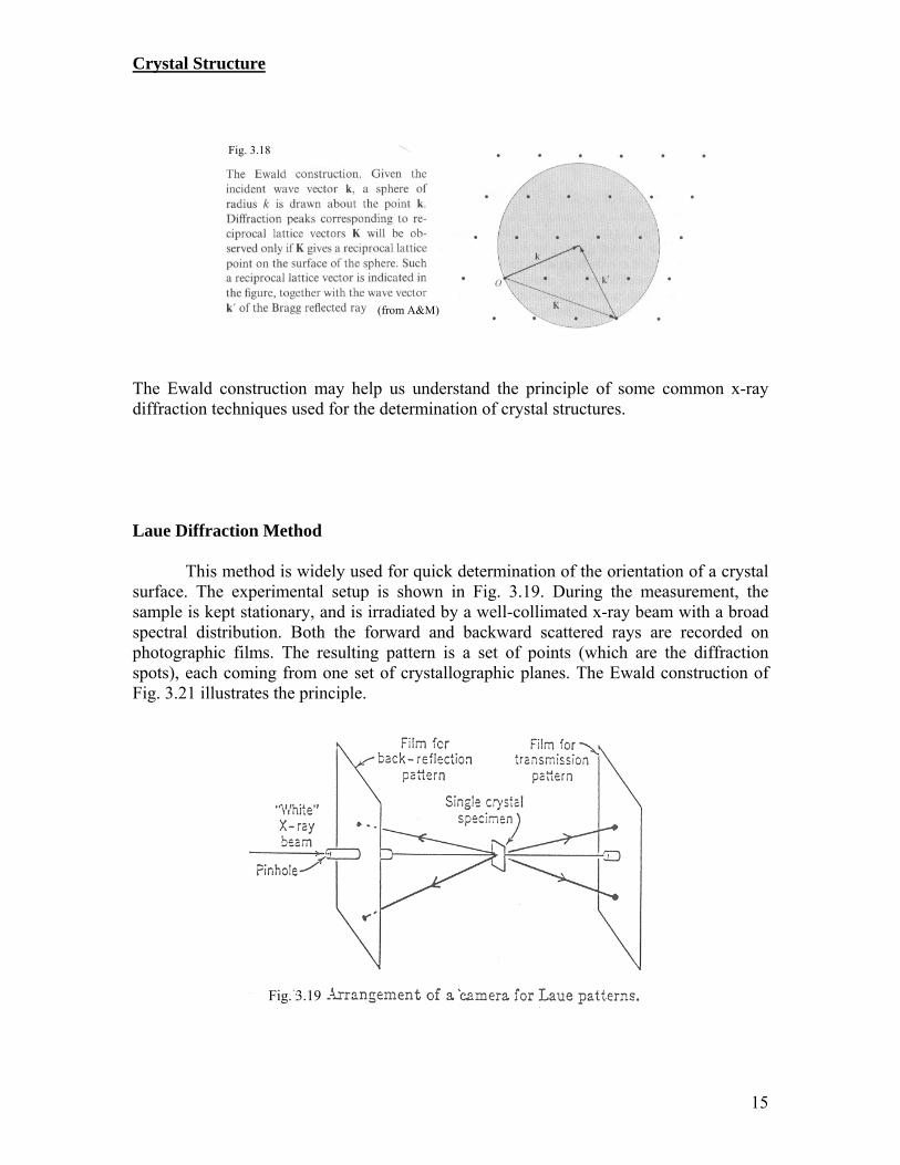
The Ewald construction may help us understand the principle of some common x-ray diffraction techniques used for the determination of crystal structures. Laue Diffraction Method

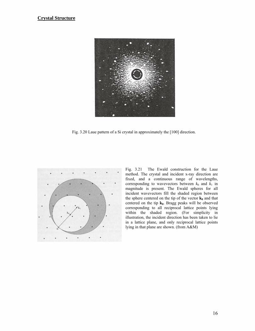
This method is widely used for quick determination of the orientation of a crystal surface. The experimental setup is shown in Fig. 3.19. During the measurement, the sample is kept stationary, and is irradiated by a well-collimated x-ray beam with a broad spectral distribution. Both the forward and backward scattered rays are recorded on photographic films. The resulting pattern is a set of points (which are the diffraction spots), each coming from one set of crystallographic planes. The Ewald construction of Fig. 3.21 illustrates the principle.

Fig. 3.19

Fig. 3.18

(from A&M)

Crystal Structure

16

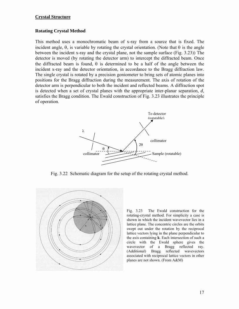
Fig. 3.21 The Ewald construction for the Laue method. The crystal and incident x-ray direction are fixed, and a continuous range of wavelengths, corresponding to wavevectors between k0 and k1 in magnitude is present. The Ewald spheres for all incident wavevectors fill the shaded region between the sphere centered on the tip of the vector k0 and that centered on the tip k0. Bragg peaks will be observed corresponding to all reciprocal lattice points lying within the shaded region. (For simplicity in illustration, the incident direction has been taken to lie in a lattice plane, and only reciprocal lattice points lying in that plane are shown. (from A&M)

Fig. 3.20 Laue pattern of a Si crystal in approximately the [100] direction.

Crystal Structure

17

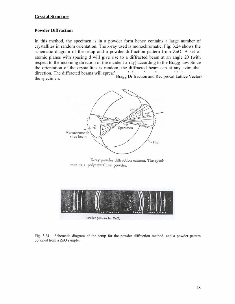
Rotating Crystal Method This method uses a monochromatic beam of x-ray from a source that is fixed. The incident angle, , is variable by rotating the crystal orientation. (Note that is the angle between the incident x-ray and the crystal plane, not the sample surface (Fig. 3.23)) The detector is moved (by rotating the detector arm) to intercept the diffracted beam. Once the diffracted beam is found, is determined to be a half of the angle between the incident x-ray and the detector orientation, in accordance to the Bragg diffraction law. The single crystal is rotated by a precision goniometer to bring sets of atomic planes into positions for the Bragg diffraction during the measurement. The axis of rotation of the detector arm is perpendicular to both the incident and reflected beams. A diffraction spot is detected when a set of crystal planes with the appropriate inter-planar separation, d, satisfies the Bragg condition. The Ewald construction of Fig. 3.23 illustrates the principle of operation.

Fig. 3.22 Schematic diagram for the setup of the rotating crystal method.

Fig. 3.23 The Ewald construction for the rotating-crystal method. For simplicity a case is shown in which the incident wavevector lies in a lattice plane. The concentric circles are the orbits swept out under the rotation by the reciprocal lattice vectors lying in the plane perpendicular to the axis containing k. Each intersection of such a circle with the Ewald sphere gives the wavevector of a Bragg reflected ray. (Additional) Bragg reflected wavevectors associated with reciprocal lattice vectors in other planes are not shown. (From A&M)

Sample (rotatable)

2 collimator

collimator

To detector (rotatable)

Crystal Structure

18

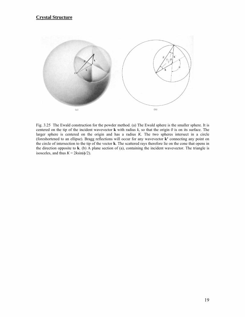
Powder Diffraction In this method, the specimen is in a powder form hence contains a large number of crystallites in random orientation. The x-ray used is monochromatic. Fig. 3.24 shows the schematic diagram of the setup and a powder diffraction pattern from ZnO. A set of atomic planes with spacing d will give rise to a diffracted beam at an angle 2 (with respect to the incoming direction of the incident x-ray) according to the Bragg law. Since the orientation of the crystallites is random, the diffracted beam can at any azimuthal direction. The diffracted beams will spread around the surface of a cone with the apex at the specimen.

Fig. 3.24 Schematic diagram of the setup for the powder diffraction method, and a powder pattern obtained from a ZnO sample.

Bragg Diffraction and Reciprocal Lattice Vectors

Crystal Structure

19

Fig. 3.25 The Ewald construction for the powder method. (a) The Ewald sphere is the smaller sphere. It is centered on the tip of the incident wavevector k with radius k, so that the origin 0 is on its surface. The larger sphere is centered on the origin and has a radius K. The two spheres intersect in a circle (foreshortened to an ellipse). Bragg reflections will occur for any wavevector k’ connecting any point on the circle of intersection to the tip of the vector k. The scattered rays therefore lie on the cone that opens in the direction opposite to k. (b) A plane section of (a), containing the incident wavevector. The triangle is isosceles, and thus K = 2ksin(/2).

Crystal Structure

20

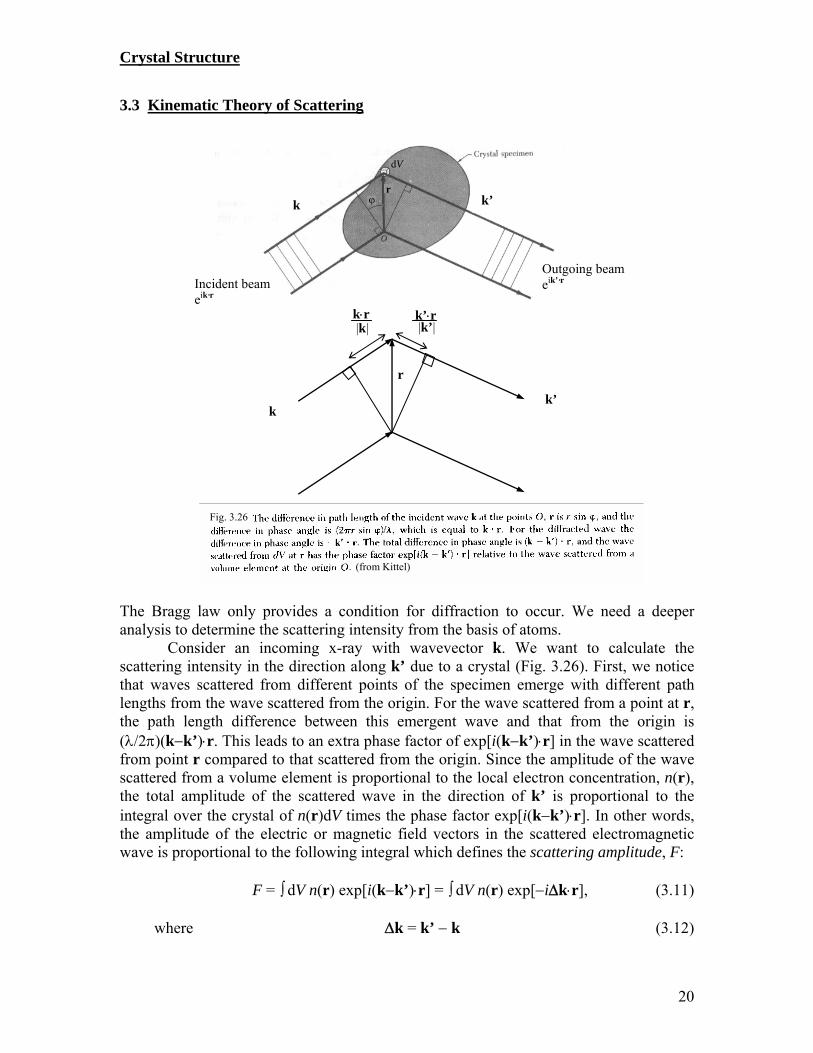
3.3 Kinematic Theory of Scattering

The Bragg law only provides a condition for diffraction to occur. We need a deeper analysis to determine the scattering intensity from the basis of atoms.

Consider an incoming x-ray with wavevector k. We want to calculate the scattering intensity in the direction along k’ due to a crystal (Fig. 3.26). First, we notice that waves scattered from different points of the specimen emerge with different path lengths from the wave scattered from the origin. For the wave scattered from a point at r, the path length difference between this emergent wave and that from the origin is (/2)(kk’)r. This leads to an extra phase factor of exp[i(kk’)r] in the wave scattered from point r compared to that scattered from the origin. Since the amplitude of the wave scattered from a volume element is proportional to the local electron concentration, n(r), the total amplitude of the scattered wave in the direction of k’ is proportional to the integral over the crystal of n(r)dV times the phase factor exp[i(kk’)r]. In other words, the amplitude of the electric or magnetic field vectors in the scattered electromagnetic wave is proportional to the following integral which defines the scattering amplitude, F:

F = dV n(r) exp[i(kk’)r] = dV n(r) exp[ikr], (3.11)

where k = k’ k (3.12)

k k’

dV

r

Incident beam eik·r

k

Outgoing beam eik’·r

(from Kittel)

Fig. 3.26

k’ k

r

kr|k| |k’|

k’r

Crystal Structure

21

To evaluate the integral in eqn. 3.11, we will exploit the fact that n(r) is periodic, i.e. invariant under translation along any lattice vectors (which must be a linear combinations of the Bravais primitive vectors, a, b, and c.) Under this condition, the Fourier expansion of n(r) will be:

G

GrGinrn

)exp()( where (3.13)

G must be such that

n(r + ma + nb + pc) = n(r) for integers m, n, p. (3.14) Here, nG is given by the Fourier transformation of n(r):

nG = (1/V) dV n(r) exp[iGr] (3.15) Eqn. 3.15 can be shown to be consistent with eqn. 3.13. We will now show that G must be a reciprocal lattice vector, i.e.

G = jA + kB + lC (3.16) where j, k, l are integers, and A, B, C are as defined in eqn. 3.6. Substitute eqn. 3.14 in eqn. 3.16, we have:

)()](exp[)exp()exp()( cpbnamrncpbnamGirGinrGinrnG

GG

G

(3.17)

Eqn. 3.17 is valid only if:

G(ma + nb + pc) = 2Mwhere M is an integer. Let’s write G as a linear combination of A, B, and C, as in eqn. 3.16, but putting no restriction on j, k, l. If we find in the end that j, k, l have to be integers, G must then be a reciprocal lattice vector. Substitute eqn. 3.16 in eqn. 3.18, and use the following relations, which are straightforward to verify:

aA = bB = cC = 2 aB = aC = bA = bC = cA = c B = 0. (3.19)

Then we have:

jm + kn + lp = M

Crystal Structure

22

Since m, n, p, and M are integers, eqn. 3.20 can be valid in general only if j, k, l are integers. This proves that G must be a reciprocal lattice vector. We now go back to the evaluation of the integral in eqn. 3.11. Substitute eqn. 3.13 in eqn. 3.11, we have:

G

GrkGindVF

])(exp[ (3.21)

= V nG (Gk) (3.22) The factor (Gk) provides an explanation to the Bragg diffraction law, namely k = GBut more informative than the Bragg diffraction law, eqn. 3.22 even tells us what the scattering amplitudes be for the various Bragg diffraction peak. In particular for the diffraction peak corresponding tok G, the scattering amplitude is just proportional to the G-component (nG) in the Fourier expansion of the sample electronic distribution. Before we continue with the calculation of F, we will divert our discussion to the important concept of Bragg diffraction of electrons at a Brillouin zone boundary. 3.31 Brillouin zone

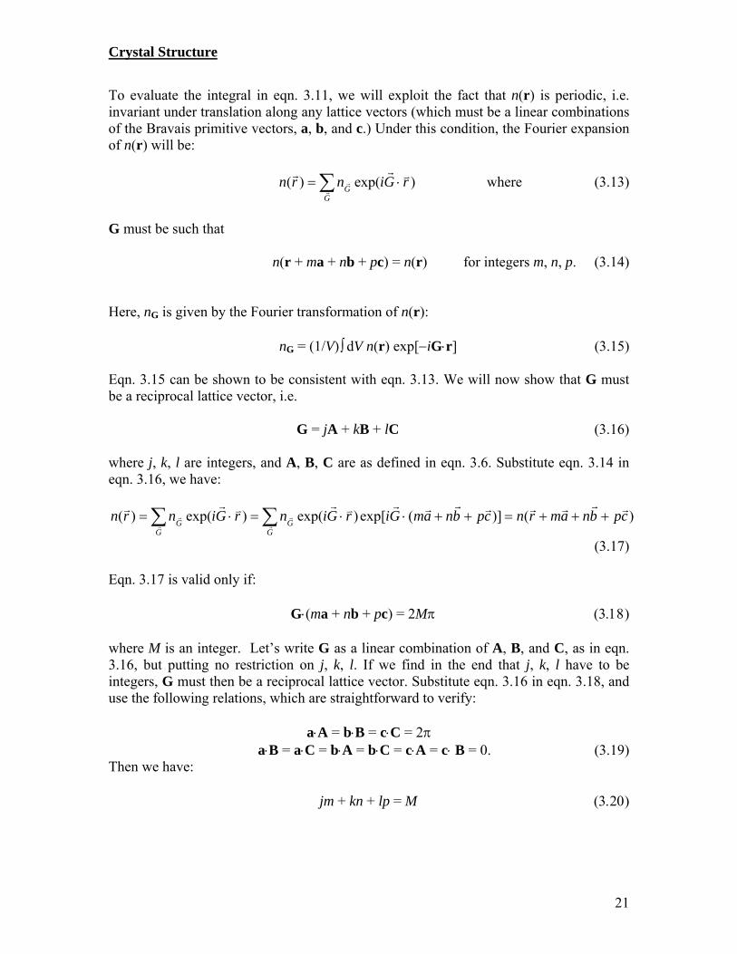
Brillouin zone is defined as a Wigner-Seitz primitive cell in the reciprocal lattice. As explained before, a Wigner-Seitz cell about a lattice point is constructed by drawing lines connecting the lattice point to all nearby points in the lattice, bisecting each line with a plane, and taking the smallest polyhedron containing the point bounded by these planes. With this construction, ½G must be perpendicular to and terminates at a

Fig. 3.27

boundary of the zone (Fig. 3.27). We will show that any wave that has wavevector, k, drawn from the origin and terminates at a zone boundary always satisfies the Bragg diffraction condition hence will be Bragg diffracted. From Fig. 3.27, it is obvious that

22

12

1 )()( GGk

(3.23)

Crystal Structure

23

According to eqn.10, the Bragg law is equivalent to:

22

12

1

2

)()(

2

2

sin2

GGk

GGk

GG

Gk

Gk

which is the same as eqn. 3.23. This proves our proposition. Since this conclusion is general to all kinds of waves, it is valid in particular to electron waves traversing in the crystal. This result says that electrons with wavevector k reaching a Brillouin zone boundary will suffer strong Bragg diffraction by the crystal planes. 3.32 Structure Factor and Form Factor Let’s now come back to the evaluation of the scattering amplitude F from eqn. 3.22. Substitute eqn. 3.15 in eqn. 3.22:

F = V nG (Gk) = dV n(r) exp[ik r]

If N is the total number of unit cells in the solid, and because the crystal is periodic,

F = N unit cell dV n(r) exp[ik r] (3.24) = N SG where SG is called the structure factor. Note that it is an integral over a unit cell, with r = 0 at one corner. It is often convenient to write the electron concentration as the superposition of electron concentration functions, nj associated with each atom j in the basis. If rj is the position vector of the atom j in the basis, our proposition means that

s

j jj rrnrn1

)()(

, (3.25)

where s is the total number of atoms in a cell. Note that the expansion of n(r) in the form of eqn. 3.25 is not unique. Particularly, it is not possible to distinguish how much charge is associated with each atom. But this in general is not a problem.

s

j jjG rkirrndVS1

)exp()(

s

j jj kindVrki1

)exp()()exp(

, (3.26)

where is defined as r rj. We now defined the atomic form factor as:

Crystal Structure

24

).exp()(

kindVf jj (3.27)

Substitute eqn. 3.27 in eqn. 3.26:

s

j jjG frkiS1

)exp(

(3.28)

Suppose, k = mA + nB + pC, (m, n, p integers) and rj = xja + yjb + zjc (x, y, z real numbers).

kr = 2(mxj + nyj + pzj) (3.29) Hence, eqn. 3.28 can be rewritten as:

s

j jjjjG pznymxifpnmS1

)(2exp(),,( (3.30)

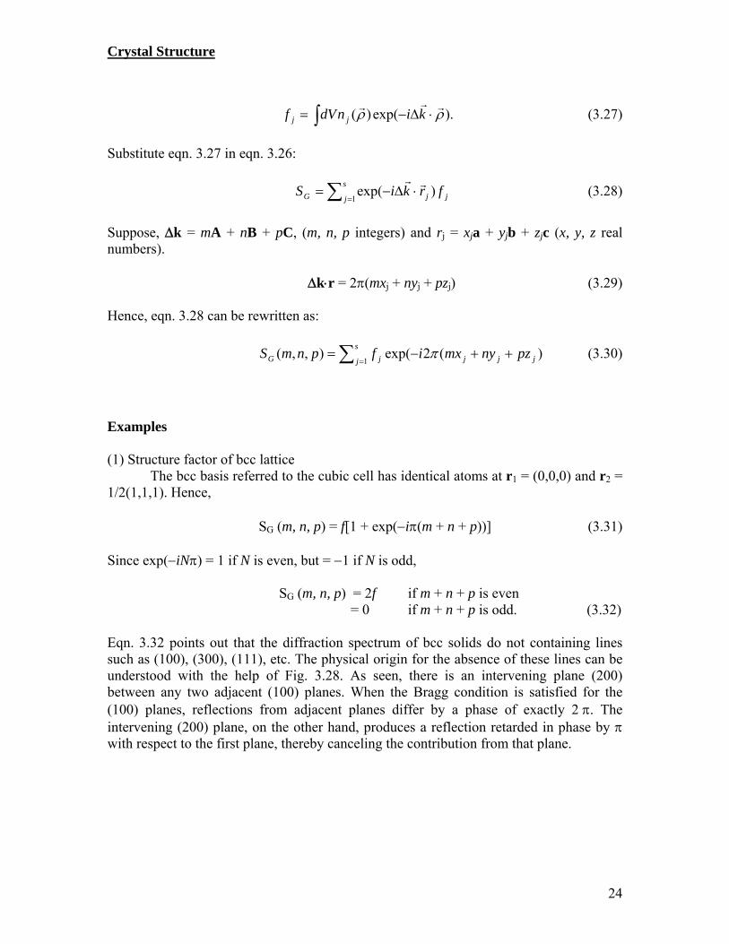
Examples (1) Structure factor of bcc lattice The bcc basis referred to the cubic cell has identical atoms at r1 = (0,0,0) and r2 = 1/2(1,1,1). Hence,

SG (m, n, p) = f[1 + exp(i(m + n + p))] (3.31) Since exp(iN) = 1 if N is even, but = 1 if N is odd,

SG (m, n, p) = 2f if m + n + p is even = 0 if m + n + p is odd. (3.32)

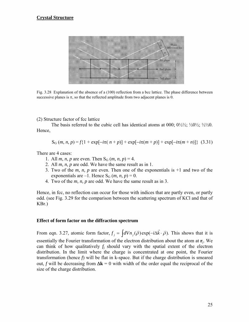
Eqn. 3.32 points out that the diffraction spectrum of bcc solids do not containing lines such as (100), (300), (111), etc. The physical origin for the absence of these lines can be understood with the help of Fig. 3.28. As seen, there is an intervening plane (200) between any two adjacent (100) planes. When the Bragg condition is satisfied for the (100) planes, reflections from adjacent planes differ by a phase of exactly 2. The intervening (200) plane, on the other hand, produces a reflection retarded in phase by with respect to the first plane, thereby canceling the contribution from that plane.

Crystal Structure

25

Fig. 3.28 Explanation of the absence of a (100) reflection from a bcc lattice. The phase difference between successive planes is , so that the reflected amplitude from two adjacent planes is 0. (2) Structure factor of fcc lattice The basis referred to the cubic cell has identical atoms at 000; 0½½; ½0½; ½½0. Hence,

SG (m, n, p) = f{1 + exp[i( n + p)] + exp[i(m + p)] + exp[i(m + n)]} (3.31) There are 4 cases:

1. All m, n, p are even. Then SG (m, n, p) = 4. 2. All m, n, p are odd. We have the same result as in 1. 3. Two of the m, n, p are even. Then one of the exponentials is +1 and two of the

exponentials are –1. Hence SG (m, n, p) = 0. 4. Two of the m, n, p are odd. We have the same result as in 3.

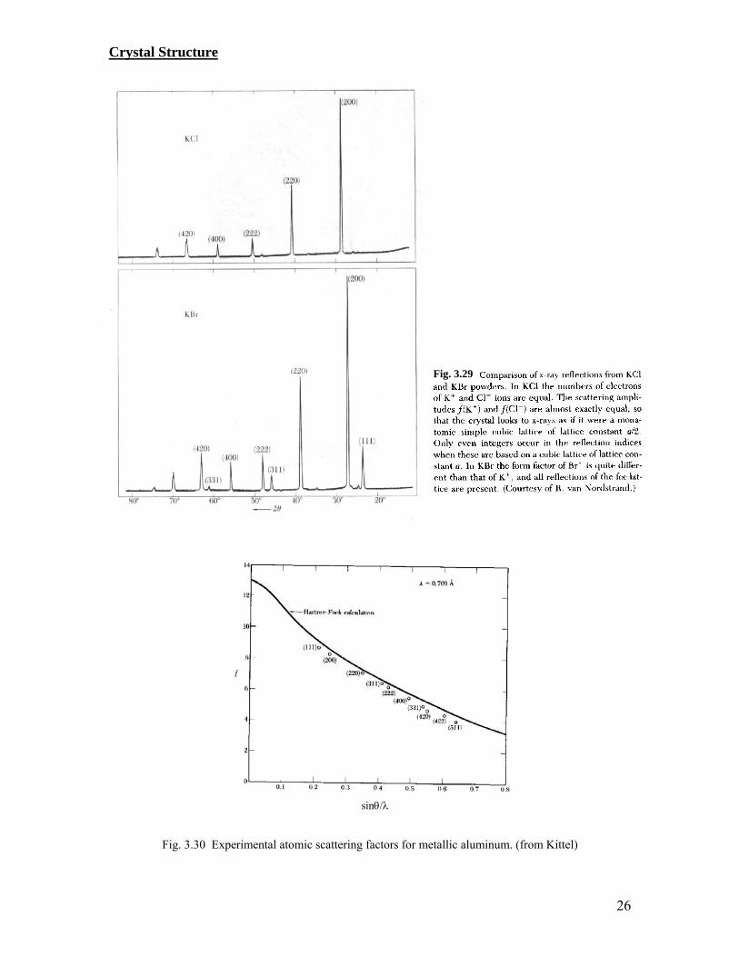
Hence, in fcc, no reflection can occur for those with indices that are partly even, or partly odd. (see Fig. 3.29 for the comparison between the scattering spectrum of KCl and that of KBr.) Effect of form factor on the diffraction spectrum

From eqn. 3.27, atomic form factor, ).exp()(

kindVf jj This shows that it is

essentially the Fourier transformation of the electron distribution about the atom at rj. We can think of how qualitatively fj should vary with the spatial extent of the electron distribution. In the limit where the charge is concentrated at one point, the Fourier transformation (hence f) will be flat in k-space. But if the charge distribution is smeared out, f will be decreasing from k = 0 with width of the order equal the reciprocal of the size of the charge distribution.

Crystal Structure

26

Fig. 3.30 Experimental atomic scattering factors for metallic aluminum. (from Kittel)

sin

Fig. 3.29