CS 179: GPU Computing

Lecture 3 / Homework 1

Recap

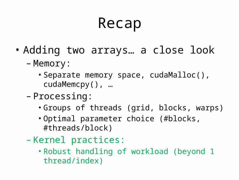
• Adding two arrays… a close look– Memory:• Separate memory space, cudaMalloc(), cudaMemcpy(),

…

– Processing:• Groups of threads (grid, blocks, warps)• Optimal parameter choice (#blocks, #threads/block)

– Kernel practices:• Robust handling of workload (beyond 1 thread/index)

Parallelization

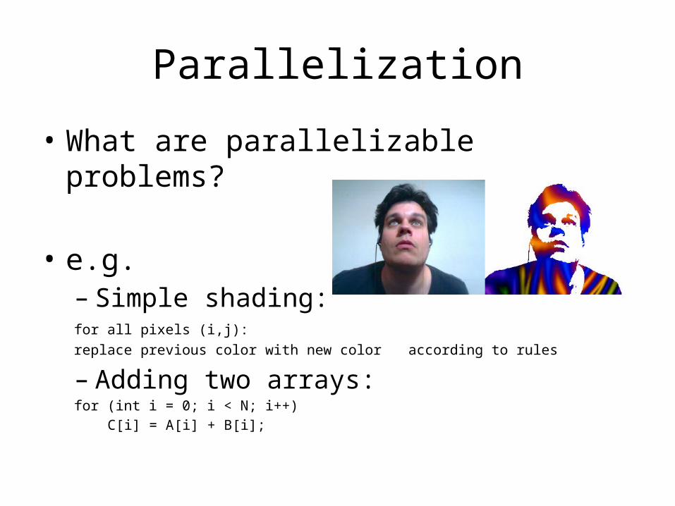
• What are parallelizable problems?

Parallelization

• What are parallelizable problems?

• e.g.– Simple shading:

for all pixels (i,j):

replace previous color with new color according to rules

– Adding two arrays:for (int i = 0; i < N; i++)

C[i] = A[i] + B[i];

Parallelization

• What aren’t parallelizable problems?– Subtle differences!

Moving Averages

http://www.ligo.org

Moving Averages

Simple Moving Average

• x[n]: input (the raw signal)• y[n]: simple moving average of x[n]

• Each point in y[n] is the average of the last K points!

Simple Moving Average

• x[n]: input (the raw signal)• y[n]: simple moving average of x[n]

• Each point in y[n] is the average of the last K points!– For all n ≥ K:

Exponential Moving Average

• Each point in y[n] follows the relation:

• “Exponential” – can expand recurrence relation:

• Each point in x[n] has an (exponentially) decaying influence!

Comparison

• Simple moving average:

– Easily parallelizable?

• Exponential moving average:

– Easily parallelizable?

Comparison

• Simple moving average:

– Easily parallelizable? Yes

• Exponential moving average:

– Easily parallelizable? Not so much

Comparison

• Simple moving average:

– Easily parallelizable? Yes

• Exponential moving average:

– Easily parallelizable? Not so much

Calculation for y[n] depends on calculation for y[n-1] !

Comparison

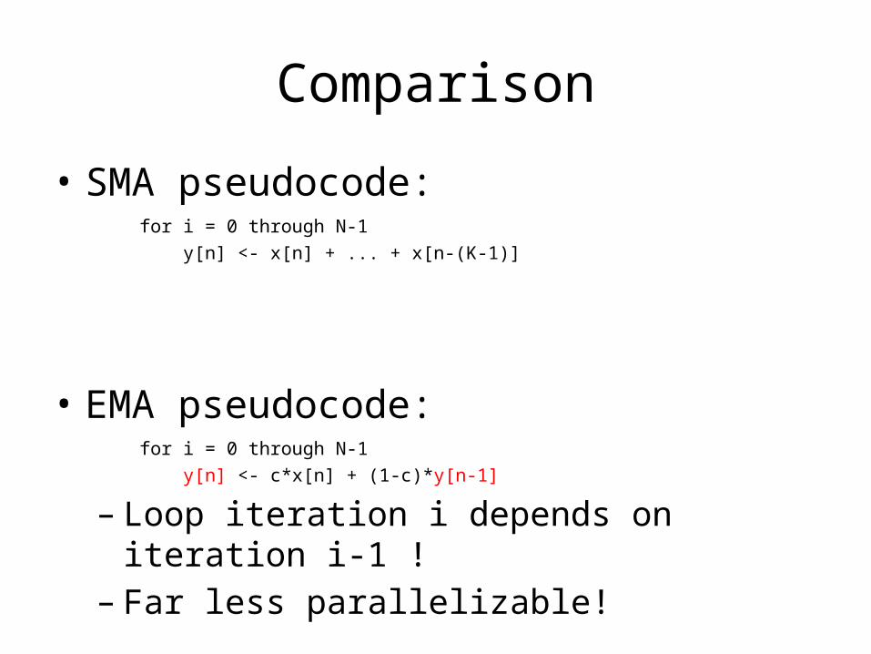
• SMA pseudocode:for i = 0 through N-1

y[n] <- x[n] + ... + x[n-(K-1)]

• EMA pseudocode:for i = 0 through N-1

y[n] <- c*x[n] + (1-c)*y[n-1]

– Loop iteration i depends on iteration i-1 !– Far less parallelizable!

Comparison

• SMA pseudocode:for i = 0 through N-1

y[n] <- x[n] + ... + x[n-(K-1)]

– Better GPU-acceleration

• EMA pseudocode:for i = 0 through N-1

y[n] <- c*x[n] + (1-c)*y[n-1]

– Loop iteration i depends on iteration i-1 !– Far less parallelizable!– Worse GPU-acceleration

Morals

• Not all problems are parallelizable!– Even similar-looking problems

• Recall: Parallel algorithms have potential in GPU computing

Small-kernel convolution

Homework 1 (coding portion)

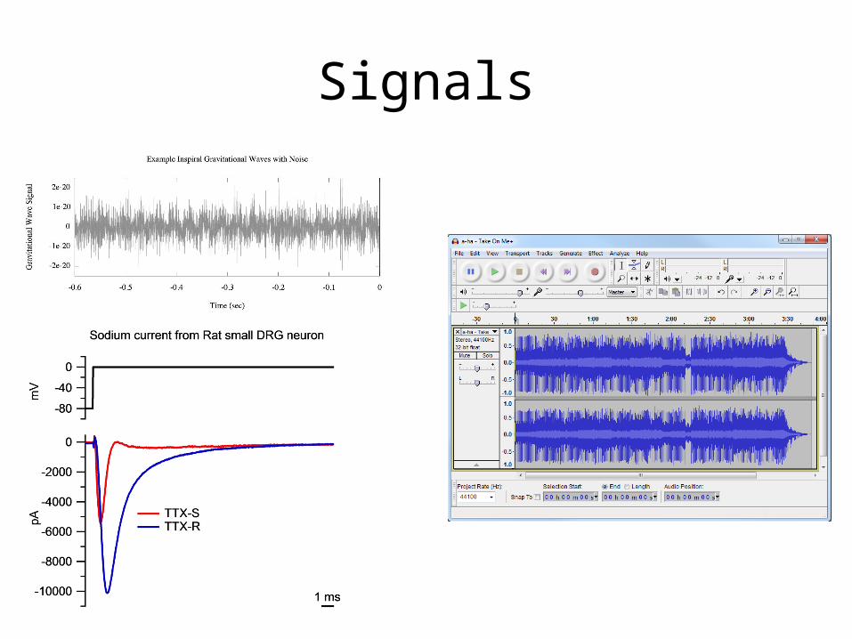
Signals

Systems

• Given input signal(s), produce output signal(s)

Discretization

• Discrete samplings• of continuous signals– Continuous audio signal -> WAV file– Voltage -> Voltage every T milliseconds

• (Will focus on discrete-time signals here)

Linear systems

• If system has:

• Then (for constants a, b):

Linear systems

• Consider a tiny piece of the signal

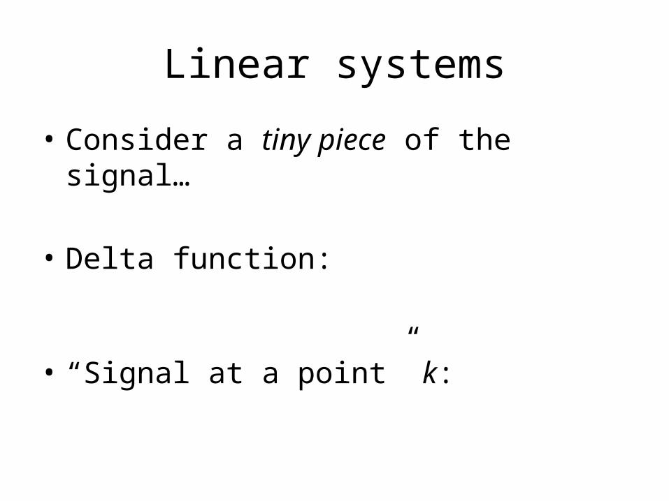
Linear systems

• Consider a tiny piece of the signal…

• Delta function:

• “Signal at a point” k:

Linear systems

• If we know that:

• Then, by linearity:

• Response at time k defined by response to delta function!

Time-invariance

• If:

• Then (for integer m):

Time-invariance

• If system has:

• Then and are time-shifted versions of each other!

Time-invariance and linearity

• Define as the impulse response to delta function:

• Then:

• And by linearity:

Time-invariance and linearity

• Can write our original signal as:

• Then, since (last slide):

• By linearity:

Morals

• “Linear time-invariant” (LTI) systems– Lots of them!

• Can be characterized entirely by

• Output given from input by:

Convolution example

• Suppose we have input , system given by

• Example output value:

Computability

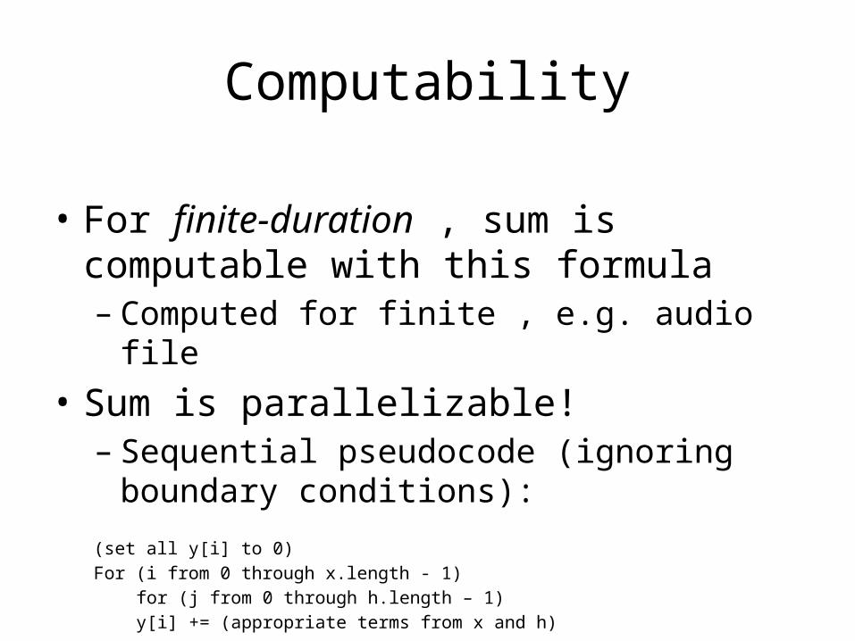
• For finite-duration , sum is computable with this formula– Computed for finite , e.g. audio file

• Sum is parallelizable!– Sequential pseudocode (ignoring boundary

conditions):

(set all y[i] to 0)For (i from 0 through x.length - 1)

for (j from 0 through h.length – 1)y[i] += (appropriate terms from x and h)

This assignment

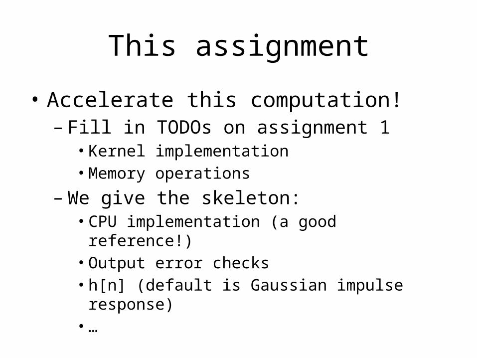
• Accelerate this computation!– Fill in TODOs on assignment 1• Kernel implementation• Memory operations

– We give the skeleton:• CPU implementation (a good reference!)• Output error checks• h[n] (default is Gaussian impulse response)• …

The code

• Framework code has two modes:– Normal mode (AUDIO_ON zero)• Generates random x[n]• Can run performance measurements on different sizes

of x[n]• Can run multiple repeated trials (adjust channels

parmeter)

– Audio mode (AUDIO_ON nonzero)• Reads input WAV file as x[n]• Outputs y[n] to WAV• Gaussian is an imperfect low-pass filter – high

frequencies attenuated!

Demonstration

Debugging tips

• Printf – Beware – you have many threads!– Set small number of threads to print

• Store intermediate results in global memory– Can copy back to host for inspection

• Check error returns!– gpuErrchk macro included – wrap around function

calls

Debugging tips

• Use small convolution test case– E.g. 5-element x[n], 3-element h[n]

Compatibility

• Our machines:– haru.caltech.edu– (We’ll try to get more up as the assignment

progresses)• CMS machines:– Only normal mode works• (Fine for this assignment)

• Your own system:– Dependencies: libsndfile (audio mode)

Administrivia

• Due date:– Wednesday, 3 PM (correction)

• Office hours (ANB 104):– Kevin/Andrew: Monday, 9-11 PM– Eric: Tuesday, 7-9 PM