1

CS 268: Lecture 9Intra-domain Routing

ProtocolsIon Stoica

Computer Science DivisionDepartment of Electrical Engineering and Computer Sciences

University of California, BerkeleyBerkeley, CA 94720-1776

(*Based in part on Aman Shaikh’s slides)

2

Internet Routing

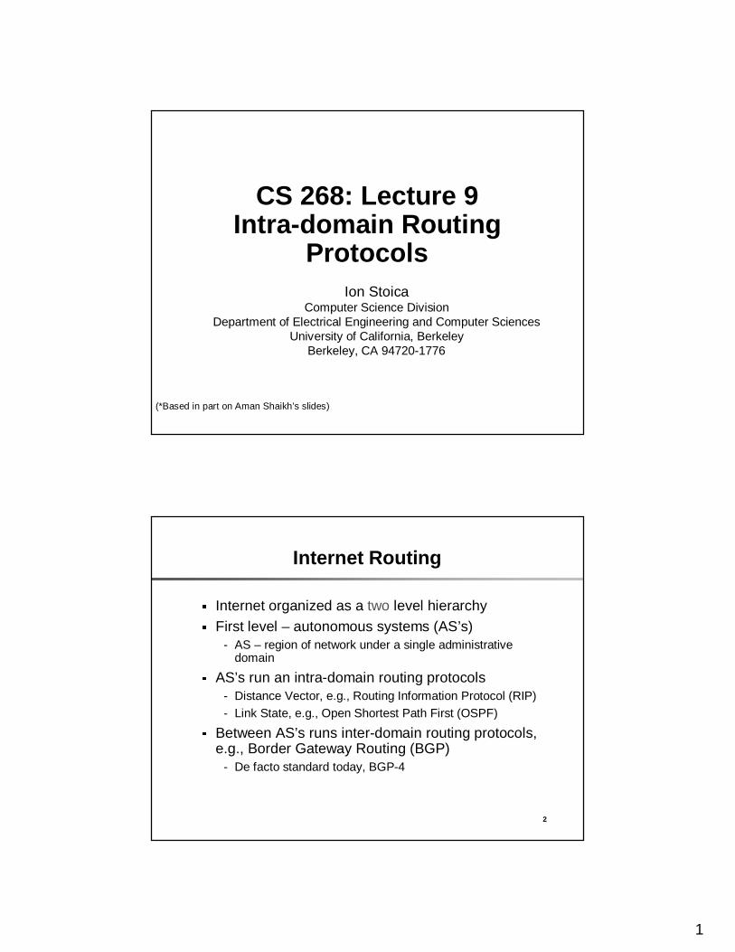
� Internet organized as a two level hierarchy� First level – autonomous systems (AS’s)

- AS – region of network under a single administrative domain

� AS’s run an intra-domain routing protocols- Distance Vector, e.g., Routing Information Protocol (RIP)- Link State, e.g., Open Shortest Path First (OSPF)

� Between AS’s runs inter-domain routing protocols, e.g., Border Gateway Routing (BGP)

- De facto standard today, BGP-4

2

3

Example

AS-1

AS-2

AS-3

Interior router

BGP router

4

Intra-domain Routing Protocols

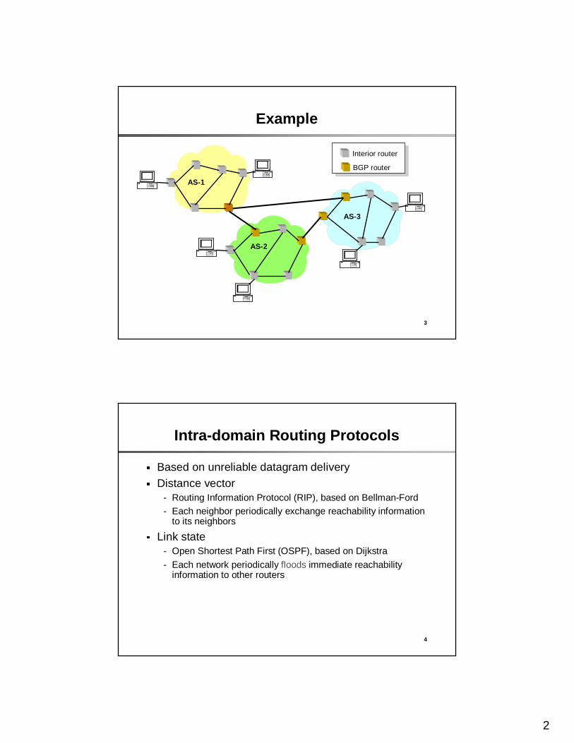
� Based on unreliable datagram delivery� Distance vector

- Routing Information Protocol (RIP), based on Bellman-Ford- Each neighbor periodically exchange reachability information

to its neighbors� Link state

- Open Shortest Path First (OSPF), based on Dijkstra

- Each network periodically floods immediate reachabilityinformation to other routers

3

5

Routing

� Goal: determine a “good” path through the network from source to destination

- Good means usually the shortest path� Network modeled as a graph

- Routers �

nodes- Link

�edges

• Edge cost: delay, congestion level,…

A

ED

CB

F

2

2

13

1

1

2

53

5

6

Routing Problem

� Assume - A network with N nodes, where each edge

is associated a cost- A node knows only its neighbors and the

cost to reach them� How does each node learns how to

reach every other node along the shortest path?

A

ED

CB

F

2

2

13

1

1

2

53

5

4

7

Distance Vector: Control Traffic� When the routing table of a node changes, the

node sends its table to its neighbors� A node updates its table with information received

from its neighbors

Host A

Host BHost E

Host D

Host C

N1 N2

N3

N4

N5

N7N6

8

Example: Distance Vector Algorithm

A C12

7

B D3

1-�D

C7C

B2B

NextHopCostDest.

Node A

D3D

C1C

A2A

NextHopCostDest.

Node B

D1D

B1B

A7A

NextHopCostDest.

Node C

C1C

B3B

-�A

NextHopCostDest.

Node D1 Initialization:2 for all neighbors V do3 if V adjacent to A4 D(A, V) = c(A,V); 5 else6 D(A, V) = � ; …

5

9

-�D

C7C

B2B

NextHopCostDest.

Node A

Example: 1st Iteration (C �

A)

A C12

7

B D3

1D3D

C1C

A2A

NextHopCostDest.

Node B

D1D

B1B

A7A

NextHopCostDest.

Node C

C1C

B3B

-�A

NextHopCostDest.

Node D(D(C,A), D(C,B), D(C,D))

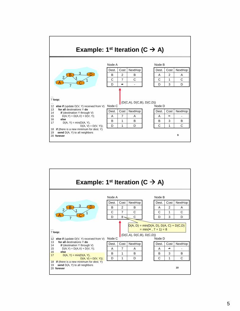
…7 loop:…12 else if (update D(V, Y) received from V) 13 for all destinations Y do14 if (destination Y through V)15 D(A,Y) = D(A,V) + D(V, Y);16 else17 D(A, Y) = min(D(A, Y),

D(A, V) + D(V, Y));18 if (there is a new minimum for dest. Y)19 send D(A, Y) to all neighbors 20 forever

10

C8D

C7C

B2B

NextHopCostDest.

Node A

Example: 1st Iteration (C �

A)

A C12

7

B D3

1D3D

C1C

A2A

NextHopCostDest.

Node B

D1D

B1B

A7A

NextHopCostDest.

Node C

C1C

B3B

-�A

NextHopCostDest.

Node D

D(A, D) = min(D(A, D), D(A, C) + D(C,D) = min( � , 7 + 1) = 8

(D(C,A), D(C,B), D(C,D))

…7 loop:…12 else if (update D(V, Y) received from V) 13 for all destinations Y do14 if (destination Y through V)15 D(A,Y) = D(A,V) + D(V, Y);16 else17 D(A, Y) = min(D(A, Y),

D(A, V) + D(V, Y));18 if (there is a new minimum for dest. Y)19 send D(A, Y) to all neighbors 20 forever

6

11

…7 loop:…12 else if (update D(V, Y) received from V) 13 for all destinations Y do14 if (destination Y through V)15 D(A,Y) = D(A,V) + D(V, Y);16 else17 D(A, Y) = min(D(A, Y),

D(A, V) + D(V, Y));18 if (there is a new minimum for dest. Y)19 send D(A, Y) to all neighbors 20 forever

C8D

C7C

B2B

NextHopCostDest.

Node A

Example: 1st Iteration (C �

A)

A C12

7

B D3

1D3D

C1C

A2A

NextHopCostDest.

Node B

D1D

B1B

A7A

NextHopCostDest.

Node C

C1C

B3B

-�A

NextHopCostDest.

Node D

12

B5D

B3C

B2B

NextHopCostDest.

Node A

Example: 1st Iteration (B�

A, C�

A)

A C12

7

B D3

1D3D

C1C

A2A

NextHopCostDest.

Node B

D1D

B1B

A7A

NextHopCostDest.

Node C

C1C

B3B

-�A

NextHopCostDest.

Node D

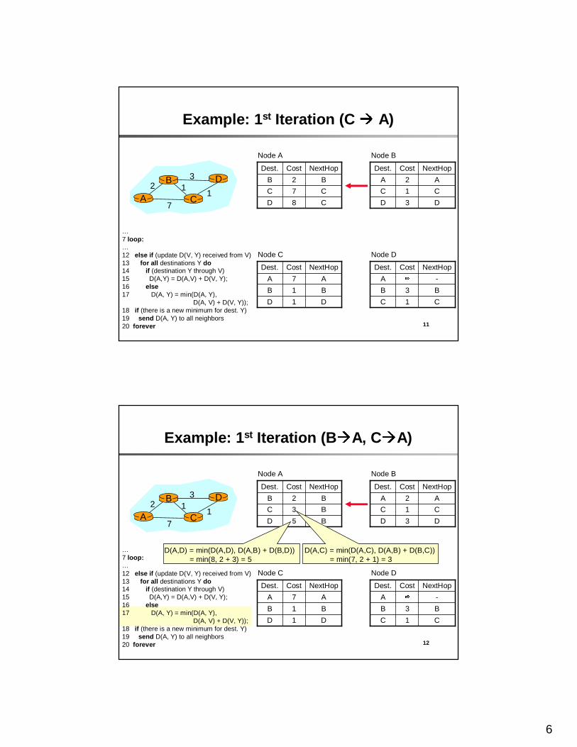
D(A,D) = min(D(A,D), D(A,B) + D(B,D))= min(8, 2 + 3) = 5

D(A,C) = min(D(A,C), D(A,B) + D(B,C)) = min(7, 2 + 1) = 3

…7 loop:…12 else if (update D(V, Y) received from V) 13 for all destinations Y do14 if (destination Y through V)15 D(A,Y) = D(A,V) + D(V, Y);16 else17 D(A, Y) = min(D(A, Y),

D(A, V) + D(V, Y));18 if (there is a new minimum for dest. Y)19 send D(A, Y) to all neighbors 20 forever

7

13

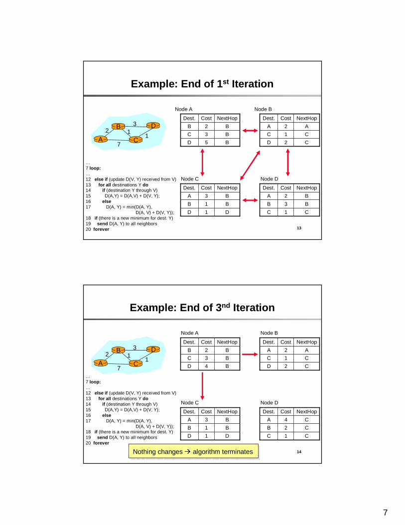
Example: End of 1st Iteration

A C12

7

B D3

1B5D

B3C

B2B

NextHopCostDest.

Node A

C2D

C1C

A2A

NextHopCostDest.

Node B

D1D

B1B

B3A

NextHopCostDest.

Node C

C1C

B3B

B2A

NextHopCostDest.

Node D

…7 loop:…12 else if (update D(V, Y) received from V) 13 for all destinations Y do14 if (destination Y through V)15 D(A,Y) = D(A,V) + D(V, Y);16 else17 D(A, Y) = min(D(A, Y),

D(A, V) + D(V, Y));18 if (there is a new minimum for dest. Y)19 send D(A, Y) to all neighbors 20 forever

14

Example: End of 3nd Iteration

A C12

7

B D3

1B4D

B3C

B2B

NextHopCostDest.

Node A

C2D

C1C

A2A

NextHopCostDest.

Node B

D1D

B1B

B3A

NextHopCostDest.

Node C

C1C

C2B

C4A

NextHopCostDest.

Node D

Nothing changes �

algorithm terminates

…7 loop:…12 else if (update D(V, Y) received from V) 13 for all destinations Y do14 if (destination Y through V)15 D(A,Y) = D(A,V) + D(V, Y);16 else17 D(A, Y) = min(D(A, Y),

D(A, V) + D(V, Y));18 if (there is a new minimum for dest. Y)19 send D(A, Y) to all neighbors 20 forever

8

15

Distance Vector: Link Cost Changes

A C14

50

B1

“goodnews travelsfast”

B1C

A4A

NCDNode B

B1B

B5A

NCDNode C

B1C

A1A

NCD

B1B

B5A

NCD

B1C

A1A

NCD

B1B

B2A

NCD

B1C

A1A

NCD

B1B

B2A

NCD

Link cost changes heretime

Algorithm terminates

7 loop:8 wait (link cost update or update message)9 if (c(A,V) changes by d) 10 for all destinations Y through V do11 D(A,Y) = D(A,Y) + d12 else if (update D(V, Y) received from V) 13 for all destinations Y do14 if (destination Y through V)15 D(A,Y) = D(A,V) + D(V, Y);16 else17 D(A, Y) = min(D(A, Y), D(A, V) + D(V, Y));18 if (there is a new minimum for destination Y)19 send D(A, Y) to all neighbors 20 forever

16

Distance Vector: Count to Infinity Problem

A C14

50

B60

“badnews travelsslowly”

B1C

A4A

NCDNode B

B1B

B5A

NCDNode C

B1C

C6A

NCD

B1B

B5A

NCD

B1C

C6A

NCD

B1B

B7A

NCD

B1C

C8A

NCD

B1B

B2A

NCD

Link cost changes here; recall from slide 24 that B also maintains shortest distance to A through C, which is 6. Thus D(B, A) becomes 6 !

time

…

7 loop:8 wait (link cost update or update message)9 if (c(A,V) changes by d) 10 for all destinations Y through V do11 D(A,Y) = D(A,Y) + d12 else if (update D(V, Y) received from V) 13 for all destinations Y do14 if (destination Y through V)15 D(A,Y) = D(A,V) + D(V, Y);16 else17 D(A, Y) = min(D(A, Y), D(A, V) + D(V, Y));18 if (there is a new minimum for destination Y)19 send D(A, Y) to all neighbors 20 forever

9

17

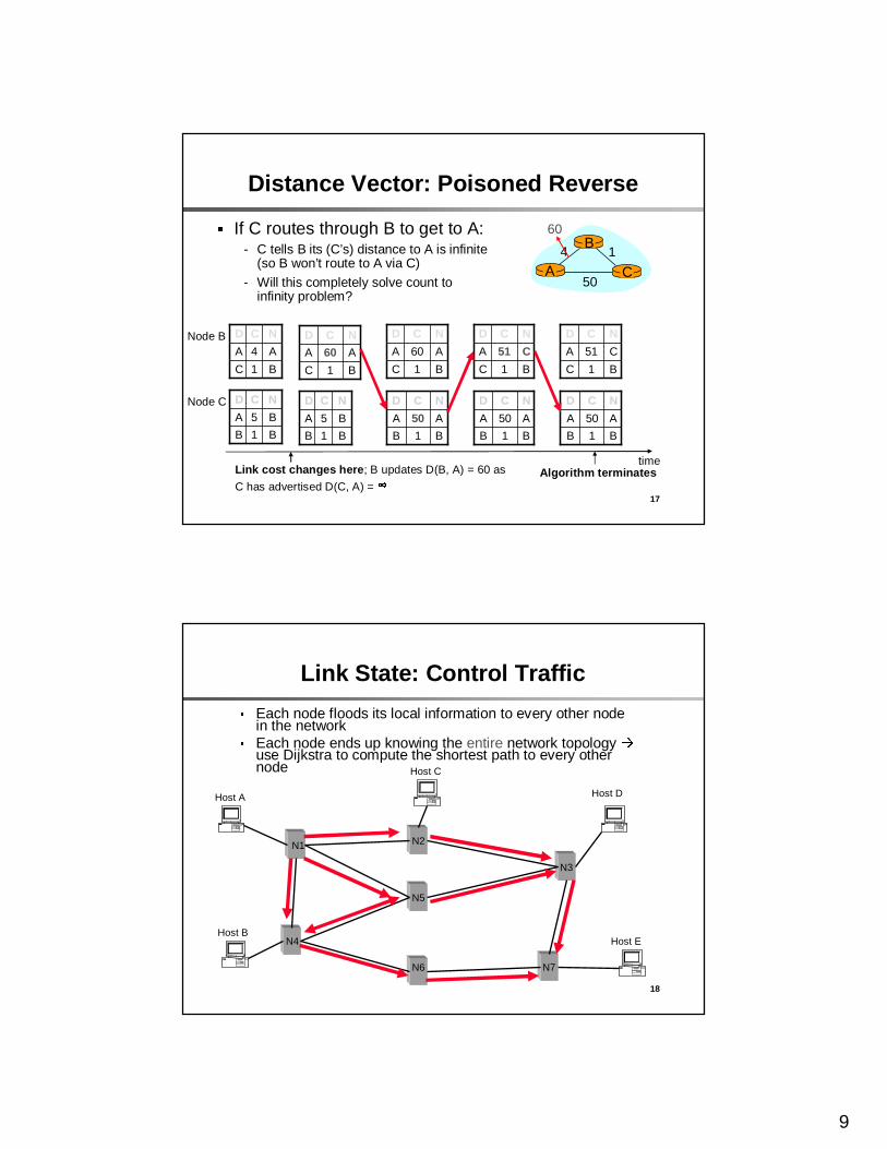
Distance Vector: Poisoned Reverse

A C14

50

B60� If C routes through B to get to A:

- C tells B its (C’s) distance to A is infinite (so B won’t route to A via C)

- Will this completely solve count to infinity problem?

B1C

A4A

NCDNode B

B1B

B5A

NCDNode C

B1C

A60A

NCD

B1B

B5A

NCD

B1B

A50A

NCD

Link cost changes here; B updates D(B, A) = 60 as

C has advertised D(C, A) = �

time

B1C

A60A

NCD

B1B

A50A

NCD

B1C

C51A

NCD

B1B

A50A

NCD

B1C

C51A

NCD

Algorithm terminates

18

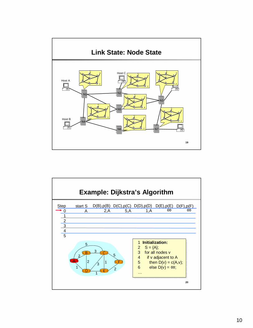
Link State: Control Traffic� Each node floods its local information to every other node

in the network� Each node ends up knowing the entire network topology

�

use Dijkstra to compute the shortest path to every other node

Host A

Host BHost E

Host D

Host C

N1 N2

N3

N4

N5

N7N6

10

19

Link State: Node State

Host A

Host BHost E

Host D

Host C

N1 N2

N3

N4

N5

N7N6

A

BE

DC

A

BE

DC A

B E

DC

A

BE

DC

A

B E

DC

A

B E

DC

A

B E

DC

20

Example: Dijkstra’s Algorithm

Step012345

start SA

D(B),p(B)2,A

D(C),p(C)5,A

D(D),p(D)1,A

D(E),p(E) D(F),p(F)

A

ED

CB

F

2

2

13

1

1

2

53

5

∞ ∞

1 Initialization:2 S = {A};3 for all nodes v4 if v adjacent to A5 then D(v) = c(A,v); 6 else D(v) = ;…

∞

11

21

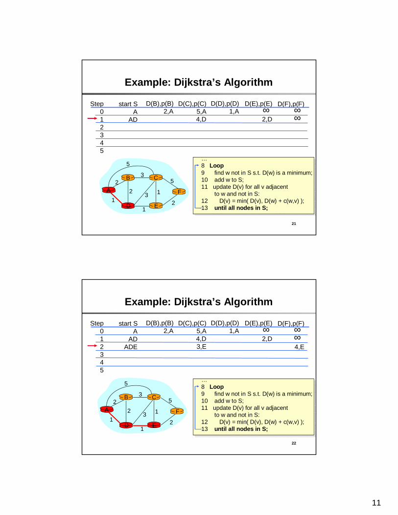
Example: Dijkstra’s Algorithm

Step012345

start SA

AD

D(B),p(B)2,A

D(C),p(C)5,A4,D

D(D),p(D)1,A

D(E),p(E)

2,D

D(F),p(F)

A

ED

CB

F

2

2

13

1

1

2

53

5

∞ ∞∞

…8 Loop9 find w not in S s.t. D(w) is a minimum; 10 add w to S; 11 update D(v) for all v adjacent

to w and not in S: 12 D(v) = min( D(v), D(w) + c(w,v) );13 until all nodes in S;

22

Example: Dijkstra’s Algorithm

Step012345

start SA

ADADE

D(B),p(B)2,A

D(C),p(C)5,A4,D3,E

D(D),p(D)1,A

D(E),p(E)

2,D

D(F),p(F)

4,E

∞ ∞∞

A

ED

CB

F

2

2

13

1

1

2

53

5…8 Loop9 find w not in S s.t. D(w) is a minimum; 10 add w to S; 11 update D(v) for all v adjacent

to w and not in S: 12 D(v) = min( D(v), D(w) + c(w,v) );13 until all nodes in S;

12

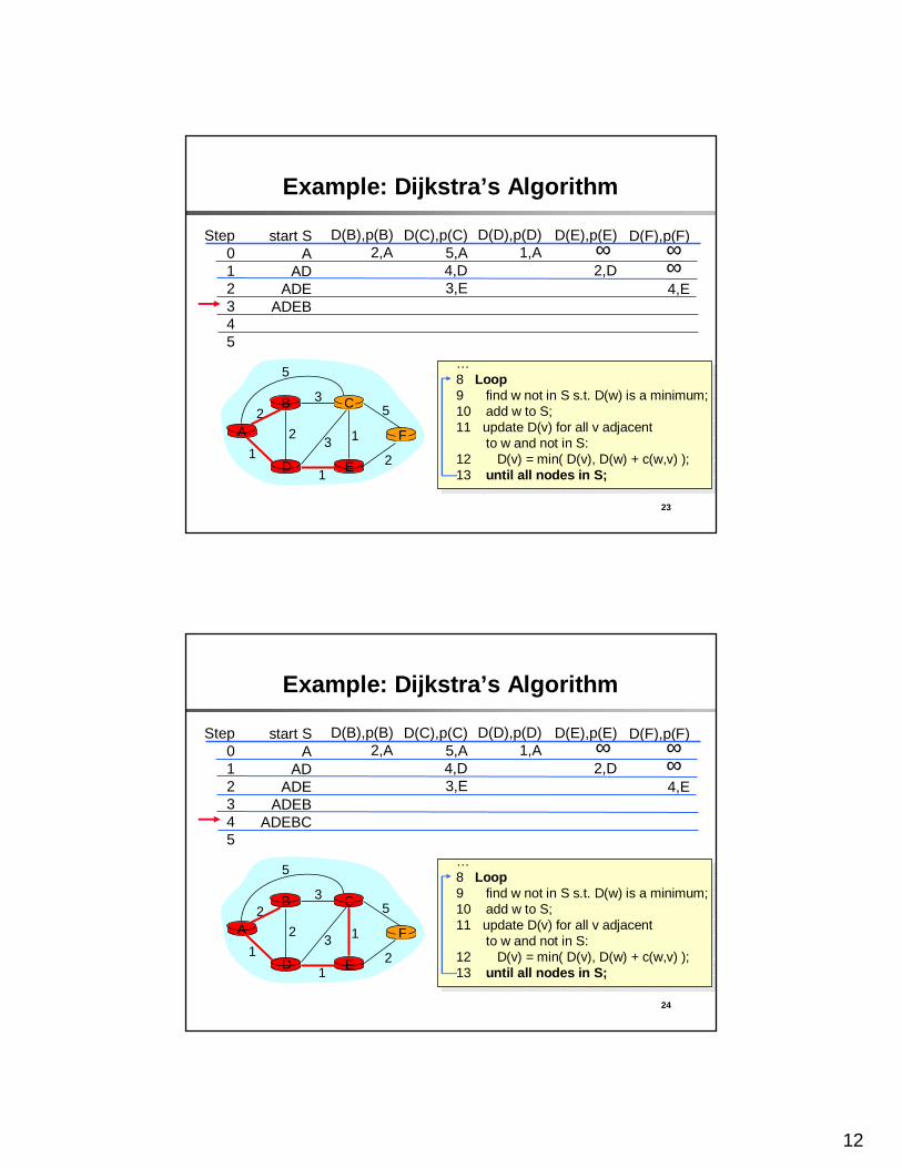
23

Example: Dijkstra’s Algorithm

Step012345

start SA

ADADE

ADEB

D(B),p(B)2,A

D(C),p(C)5,A4,D3,E

D(D),p(D)1,A

D(E),p(E)

2,D

D(F),p(F)

4,E

∞ ∞∞

A

ED

CB

F

2

2

13

1

1

2

53

5…8 Loop9 find w not in S s.t. D(w) is a minimum; 10 add w to S; 11 update D(v) for all v adjacent

to w and not in S: 12 D(v) = min( D(v), D(w) + c(w,v) );13 until all nodes in S;

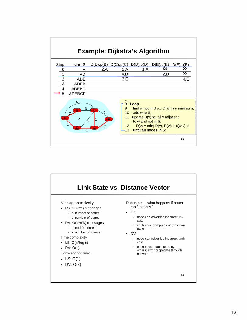
24

Example: Dijkstra’s Algorithm

Step012345

start SA

ADADE

ADEBADEBC

D(B),p(B)2,A

D(C),p(C)5,A4,D3,E

D(D),p(D)1,A

D(E),p(E)

2,D

D(F),p(F)

4,E

∞ ∞∞

A

ED

CB

F

2

2

13

1

1

2

53

5…8 Loop9 find w not in S s.t. D(w) is a minimum; 10 add w to S; 11 update D(v) for all v adjacent

to w and not in S: 12 D(v) = min( D(v), D(w) + c(w,v) );13 until all nodes in S;

13

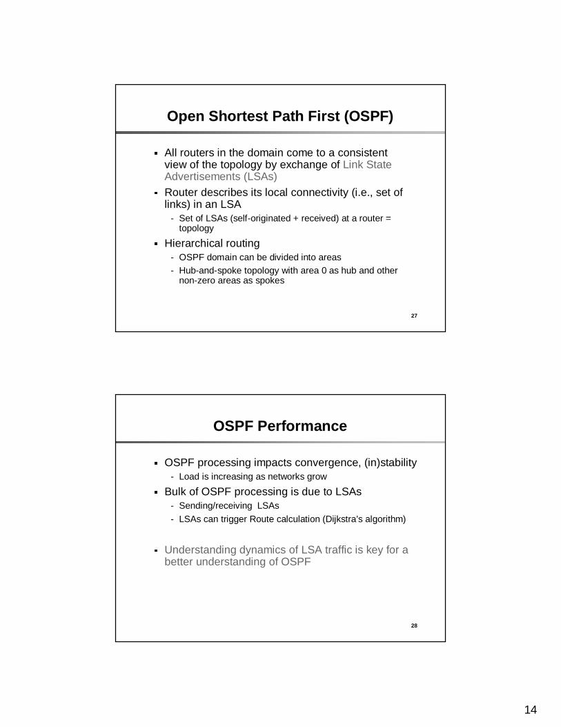
25

Example: Dijkstra’s Algorithm

Step012345

start SA

ADADE

ADEBADEBC

ADEBCF

D(B),p(B)2,A

D(C),p(C)5,A4,D3,E

D(D),p(D)1,A

D(E),p(E)

2,D

D(F),p(F)

4,E

∞ ∞∞

A

ED

CB

F

2

2

13

1

1

2

53

5…8 Loop9 find w not in S s.t. D(w) is a minimum; 10 add w to S; 11 update D(v) for all v adjacent

to w and not in S: 12 D(v) = min( D(v), D(w) + c(w,v) );13 until all nodes in S;

26

Link State vs. Distance Vector

Message complexity� LS: O(n2*e) messages

- n: number of nodes

- e: number of edges� DV: O(d*n*k) messages

- d: node’s degree

- k: number of rounds

Time complexity� LS: O(n*log n) � DV: O(n)

Convergence time� LS: O(1)� DV: O(k)

Robustness: what happens if router malfunctions?

� LS: - node can advertise incorrect link

cost

- each node computes only its owntable

� DV:- node can advertise incorrect path

cost

- each node’s table used by others; error propagate through network

14

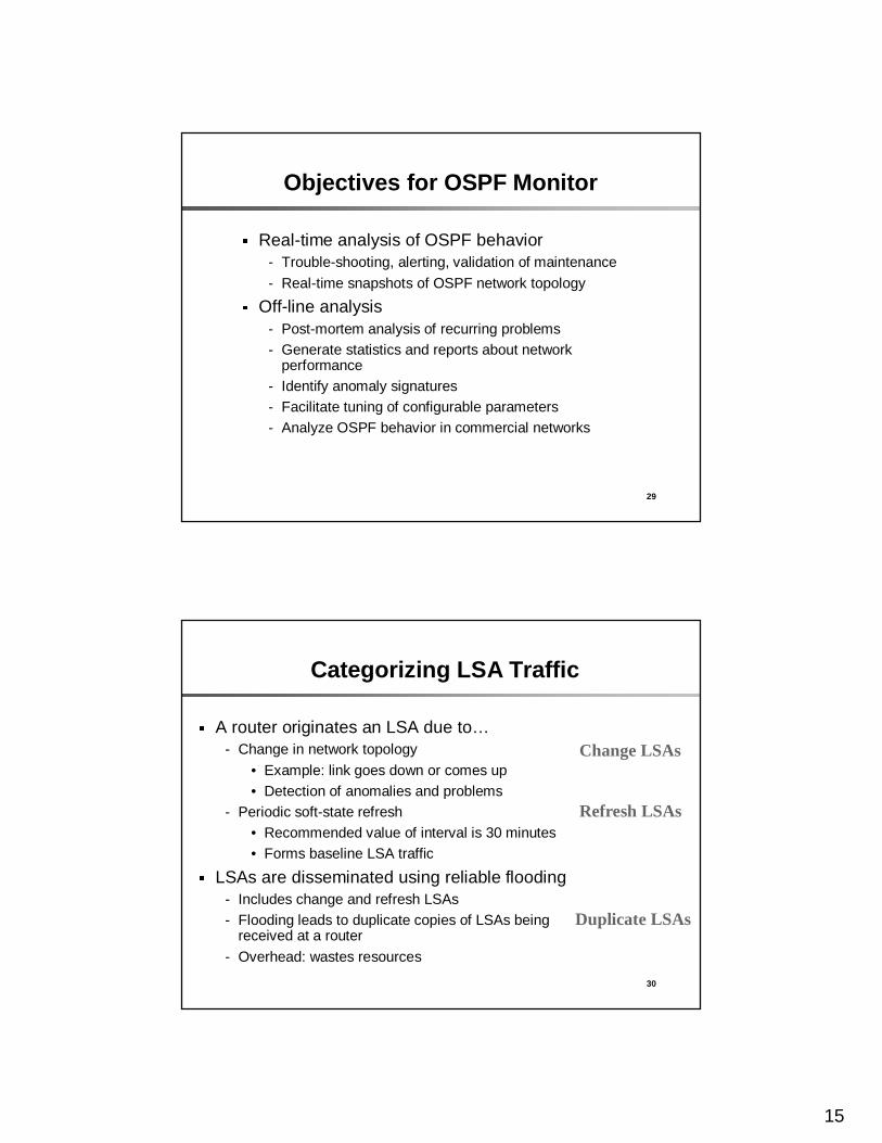
27

Open Shortest Path First (OSPF)

� All routers in the domain come to a consistent view of the topology by exchange of Link State Advertisements (LSAs)

� Router describes its local connectivity (i.e., set of links) in an LSA

- Set of LSAs (self-originated + received) at a router = topology

� Hierarchical routing- OSPF domain can be divided into areas- Hub-and-spoke topology with area 0 as hub and other

non-zero areas as spokes

28

OSPF Performance

� OSPF processing impacts convergence, (in)stability- Load is increasing as networks grow

� Bulk of OSPF processing is due to LSAs- Sending/receiving LSAs

- LSAs can trigger Route calculation (Dijkstra’s algorithm)

� Understanding dynamics of LSA traffic is key for a better understanding of OSPF

15

29

Objectives for OSPF Monitor

� Real-time analysis of OSPF behavior- Trouble-shooting, alerting, validation of maintenance

- Real-time snapshots of OSPF network topology� Off-line analysis

- Post-mortem analysis of recurring problems- Generate statistics and reports about network

performance- Identify anomaly signatures- Facilitate tuning of configurable parameters- Analyze OSPF behavior in commercial networks

30

Categorizing LSA Traffic

� A router originates an LSA due to…- Change in network topology

• Example: link goes down or comes up• Detection of anomalies and problems

- Periodic soft-state refresh• Recommended value of interval is 30 minutes• Forms baseline LSA traffic

� LSAs are disseminated using reliable flooding- Includes change and refresh LSAs- Flooding leads to duplicate copies of LSAs being

received at a router

- Overhead: wastes resources

Change LSAs

Refresh LSAs

Duplicate LSAs

16

31

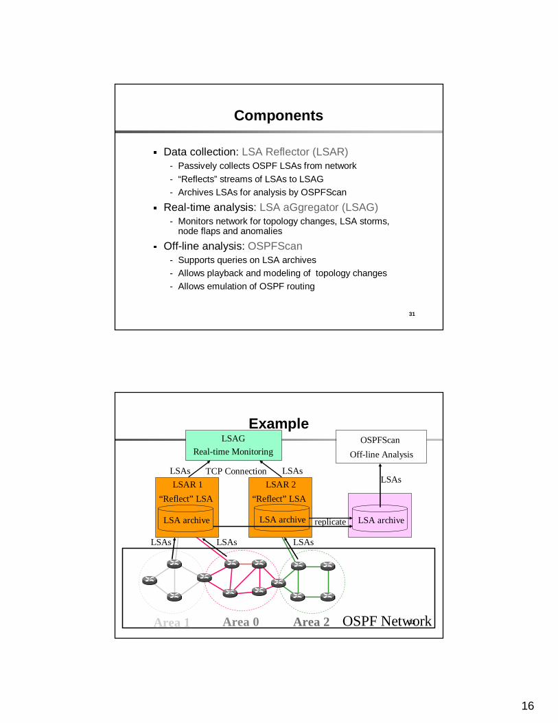
Components

� Data collection: LSA Reflector (LSAR)- Passively collects OSPF LSAs from network

- “Reflects” streams of LSAs to LSAG- Archives LSAs for analysis by OSPFScan

� Real-time analysis: LSA aGgregator (LSAG)- Monitors network for topology changes, LSA storms,

node flaps and anomalies� Off-line analysis: OSPFScan

- Supports queries on LSA archives- Allows playback and modeling of topology changes- Allows emulation of OSPF routing

32

Example

Area 0Area 1 Area 2

Real-time Monitoring

LSAG

“Reflect” LSA

LSA archive

LSAR 1

“Reflect” LSA

LSAR 2

OSPFScan

Off-line Analysis

replicateLSA archive LSA archive

OSPF Network

LSAsLSAsLSAs

LSAs LSAs LSAs

TCP Connection

17

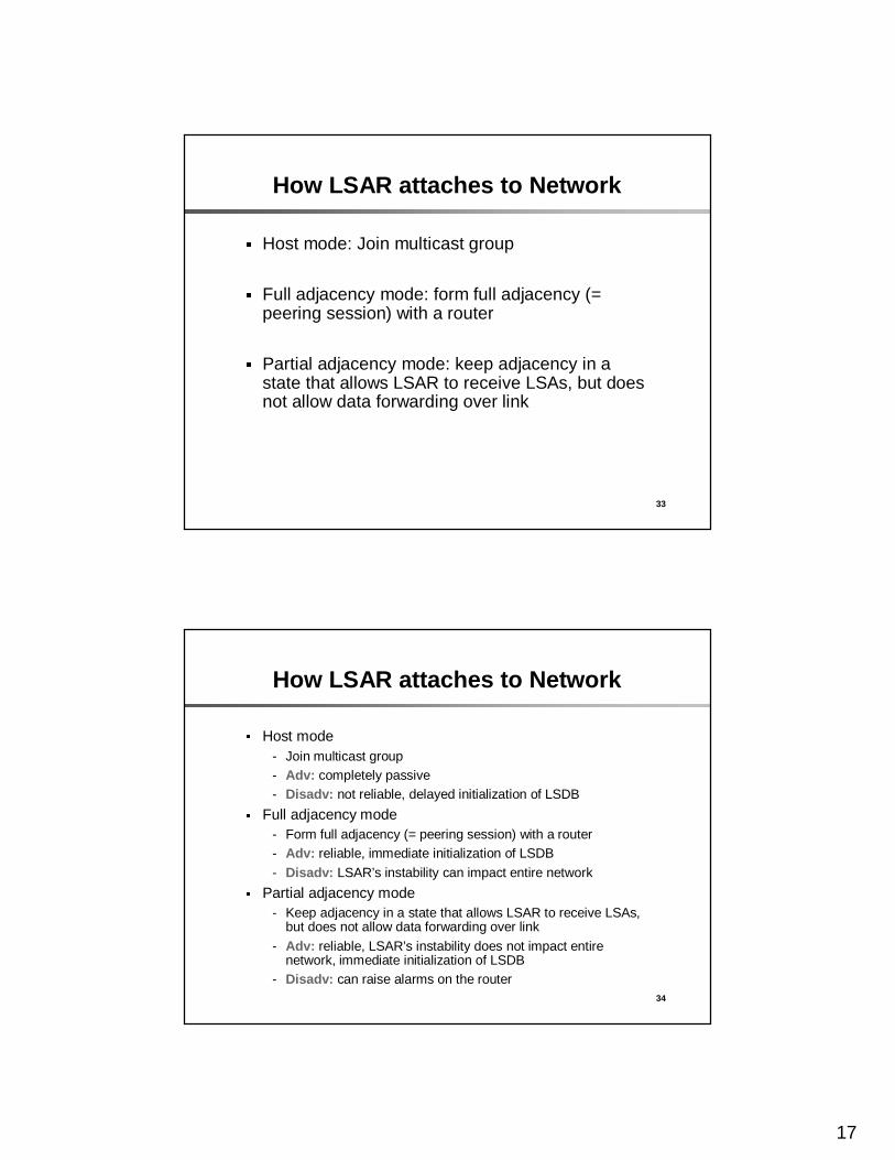
33

How LSAR attaches to Network

� Host mode: Join multicast group

� Full adjacency mode: form full adjacency (= peering session) with a router

� Partial adjacency mode: keep adjacency in a state that allows LSAR to receive LSAs, but does not allow data forwarding over link

34

How LSAR attaches to Network

� Host mode- Join multicast group- Adv: completely passive- Disadv: not reliable, delayed initialization of LSDB

� Full adjacency mode- Form full adjacency (= peering session) with a router- Adv: reliable, immediate initialization of LSDB

- Disadv: LSAR’s instability can impact entire network� Partial adjacency mode

- Keep adjacency in a state that allows LSAR to receive LSAs, but does not allow data forwarding over link

- Adv: reliable, LSAR’s instability does not impact entire network, immediate initialization of LSDB

- Disadv: can raise alarms on the router

18

35

Partial Adjacency for LSAR

LSAR

Partial state

I have LSA L

Please send me LSA LPlease send me LSA LPlease send me LSA L

I need LSA L from LSAR

• LSAR↔R link is not used for data forwarding

R

• Router R does not advertise a link to LSAR

• Routers (except R) not aware of LSAR’s presence• Does not trigger routing calculations in network• LSAR’s going up/down does not impact network

• LSAR does not originate any LSAs

36

Performance Evaluation

� Performance of LSAR and LSAG through lab experiments

- LSAR and LSAG are key to real-time monitoring� How performance scales with LSA-rate and

network size

19

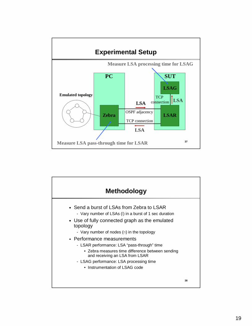
37

Experimental Setup

LSALSA

PC

ZebraOSPF adjacency

TCP connection

SUT

LSAR

LSAG

TCP connection LSA

LSA

Emulated topology

LSA

Measure LSA pass-through time for LSAR

Measure LSA processing time for LSAG

38

Methodology

� Send a burst of LSAs from Zebra to LSAR- Vary number of LSAs (l) in a burst of 1 sec duration

� Use of fully connected graph as the emulated topology

- Vary number of nodes (n) in the topology� Performance measurements

- LSAR performance: LSA “pass-through” time• Zebra measures time difference between sending

and receiving an LSA from LSAR- LSAG performance: LSA processing time

• Instrumentation of LSAG code

20

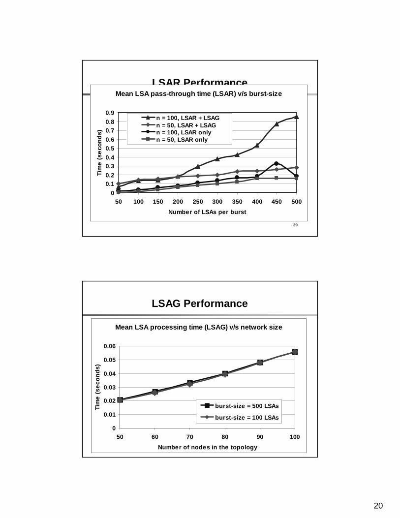
39

LSAR PerformanceMean LSA pass-through time (LSAR) v/s burst-size

0

0.10.2

0.30.4

0.50.6

0.70.8

0.9

50 100 150 200 250 300 350 400 450 500

Number of LSAs per burst

Tim

e (

seco

nd

s)

n = 100, LSAR + LSAGn = 50, LSAR + LSAGn = 100, LSAR onlyn = 50, LSAR only

40

LSAG Performance

Mean LSA processing time (LSAG) v/s network size

0

0.01

0.02

0.03

0.04

0.05

0.06

50 60 70 80 90 100

Number of nodes in the topology

Tim

e (

seco

nd

s)

burst-size = 500 LSAs

burst-size = 100 LSAs

21

41

Enterprise Network Case Study

� The network provides customers with connectivity to applications and databases residing in the data center

� OSPF network- 15 areas, 500 routers

• This case study covers 8 areas, 250 routers• One month: April 2002

- Link-layer = Ethernet-based LANs� Customers are connected via leased lines

- Customer routes are injected via EIGRP into OSPF• The routes are propagated via external LSAs• Quite reasonable for the enterprise network in question

42

Enterprise Network Topology

Area 0Area B Area C

Area A

ServersDatabase Applications

CustomerCustomer

OSPFDomain

Customer

B1 B2

Monitor

LAN1 LAN2

Border rtrs

Area A

Area 0

External(EIGRP)

Monitor is completely passiveNo adjacencies with any routersReceives LSAs on a multicast group

22

43

Highlights of the Results

� Categorize, baseline and predict- Categories: Refresh, Change, Duplicate; External, Internal

- Bulk of LSA traffic is due to refresh

- Refresh LSA traffic is smooth: no evidence of refresh synchronization across network

- Refresh LSA traffic is predictable from router configuration info� Detect, diagnose and act

- Almost all LSAs arise from persistent yet partial failure modes

- Internal LSA spikes

• Indicate router hardware degradation

• Carry out preventive maintenance

- External LSA spikes

• Indicate degradation in customer connectivity

• Call customer before customer calls you� Propose Improvements

- Simple configuration changes to reduce duplicate LSA traffic

44

0

4000

8000

1 11 21

Area 4Days

0

4000

8000

1 11 21

Area 3Days

0

4000

8000

1 11 21

Area 2

Days1

100

10000

1000000

1 11 21

Area 0

Days

LSA Traffic in Different Areas

DuplicateLSAs

Change LSAs

Refresh LSAs

Artifact: 23 hr day (Apr 7)

Genuine AnomalyGenuine Anomaly

23

45

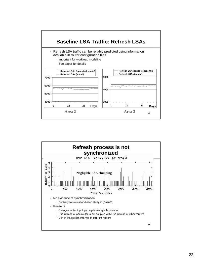
Baseline LSA Traffic: Refresh LSAs� Refresh LSA traffic can be reliably predicted using information

available in router configuration files- Important for workload modeling - See paper for details

4000

5000

6000

7000

1 11 21

Refresh LSAs (ex pected:config)Refresh LSAs (actual)

Area 2

3000

4000

5000

1 11 21

Refresh LSAs (expected:config)Refresh LSAs (actual)

Area 3DaysDays

46

Refresh process is not synchronized

� No evidence of synchronization- Contrary to simulation-based study in [Basu01]

� Reasons- Changes in the topology help break synchronization

- LSA refresh at one router is not coupled with LSA refresh at other routers

- Drift in the refresh interval of different routers

Negligible LSA clumping

24

47

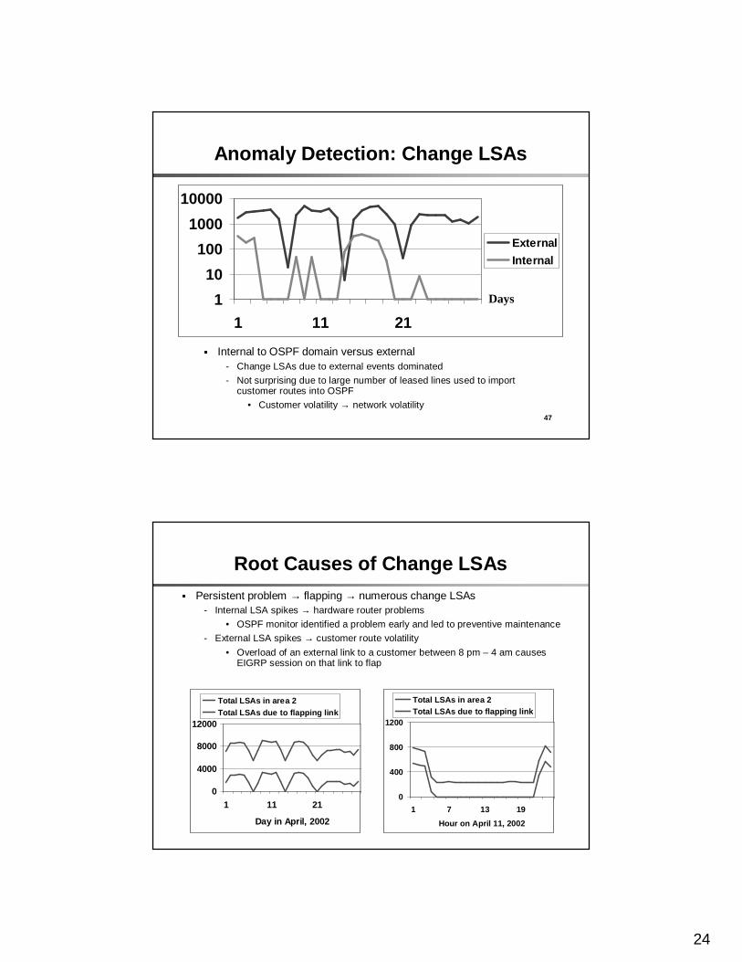
Anomaly Detection: Change LSAs

� Internal to OSPF domain versus external- Change LSAs due to external events dominated

- Not surprising due to large number of leased lines used to import customer routes into OSPF

• Customer volatility → network volatility

1

10

100

1000

10000

1 11 21

External

Internal

Days

48

Root Causes of Change LSAs� Persistent problem → flapping → numerous change LSAs

- Internal LSA spikes → hardware router problems

• OSPF monitor identified a problem early and led to preventive maintenance

- External LSA spikes → customer route volatility

• Overload of an external link to a customer between 8 pm – 4 am causes EIGRP session on that link to flap

0

400

800

1200

1 7 13 19

Hour on April 11, 2002

Total LSAs in area 2Total LSAs due to flapping link

0

4000

8000

12000

1 11 21

Day in April, 2002

Total LSAs in area 2Total LSAs due to flapping link

25

49

Overhead: Duplicate LSAs

� Why do some areas witness substantial duplicate LSA traffic, while other areas do not witness any?

- OSPF flooding over LANs leads to control plane asymmetries and to imbalances in duplicate LSA traffic

-50

950

1950

2950

1 11 21

Duplicate LSAs in area 3Duplicate LSAs in area 2

Days

50

OSPF Operations over Broadcast Networks

1) Each node sends an LSA to multicast group DR-rtrs- Both designated router (DR) and backup designated router

BDR subscribe to this group

2) DR floods the LSA back to all routers on the network- Send to all-rtrs multicast group to which all nodes subscribe

DR BDR

DR BDR

26

51

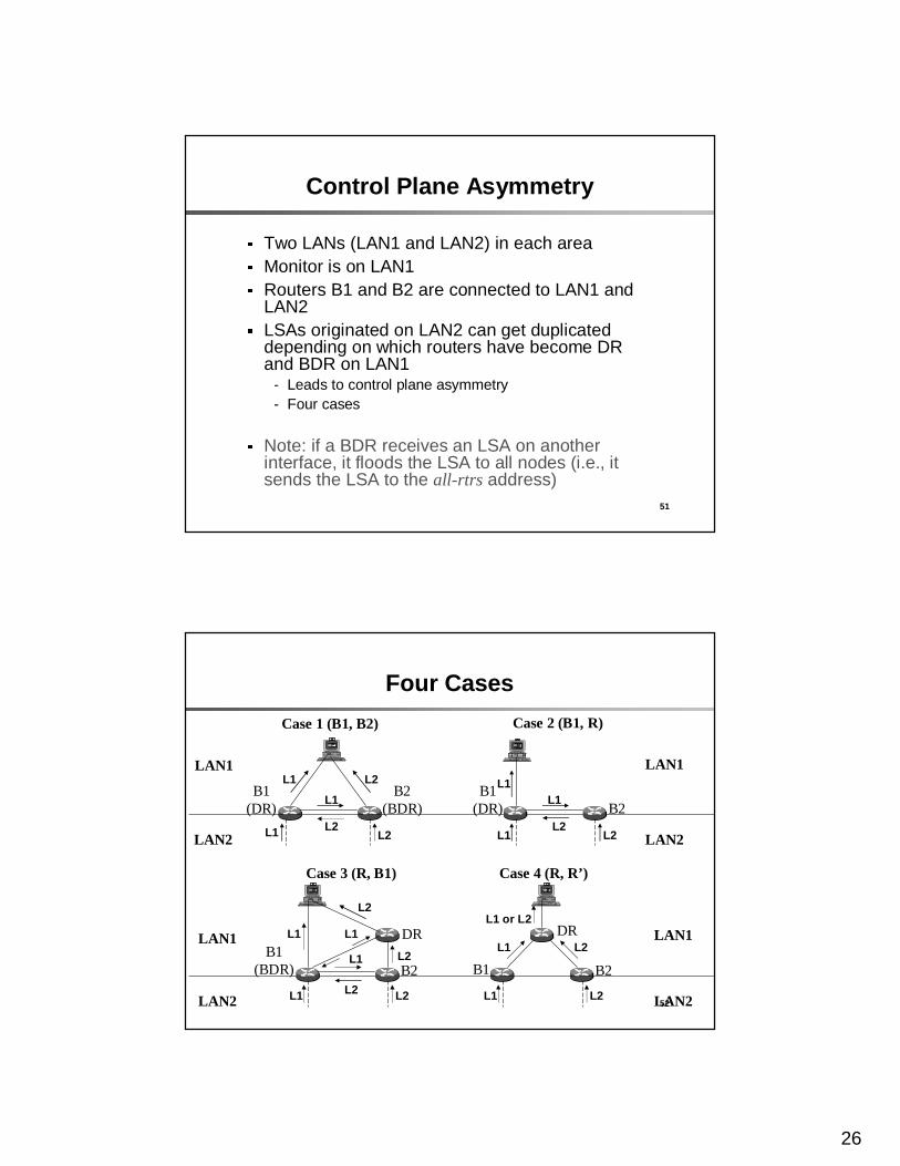
Control Plane Asymmetry

� Two LANs (LAN1 and LAN2) in each area� Monitor is on LAN1� Routers B1 and B2 are connected to LAN1 and

LAN2� LSAs originated on LAN2 can get duplicated

depending on which routers have become DR and BDR on LAN1

- Leads to control plane asymmetry- Four cases

� Note: if a BDR receives an LSA on another interface, it floods the LSA to all nodes (i.e., it sends the LSA to the all-rtrs address)

52

Four Cases

B1(DR)

B2(BDR)

LAN1

LAN2

Case 1 (B1, B2)

B1(DR) B2

Case 2 (B1, R)

LAN1

LAN2

L1 L2

L1

L1 L2L2

L1

L2L2L1

L1

B2B1

DR

LAN2

LAN1

LAN2

Case 4 (R, R’ )

LAN1B1

(BDR) B2

DR

Case 3 (R, B1)

L1

L1 L1

L1

L2 L2

L2

L2

L1 L2

L2L1

L1 or L2

27

53

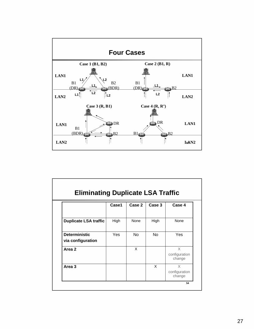
Four Cases

B2B1

DR

LAN2

LAN1

LAN2

Case 4 (R, R’ )

LAN1B1

(BDR) B2

DR

Case 3 (R, B1)

B1(DR)

B2(BDR)

LAN1

LAN2

Case 1 (B1, B2)

B1(DR) B2

Case 2 (B1, R)

LAN1

LAN2

L1 L2

L1

L1 L2L2 L2

L1

54

Eliminating Duplicate LSA Traffic

X configuration

change

XArea 3

X configuration

change

XArea 2

YesNoNoYesDeterministic via configuration

NoneHighNoneHighDuplicate LSA traffic

Case 4Case 3Case 2 Case1

28

55

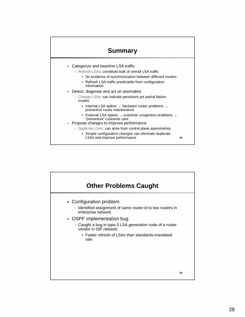
Summary

� Categorize and baseline LSA traffic- Refresh LSAs: constitute bulk of overall LSA traffic

• No evidence of synchronization between different routers• Refresh LSA traffic predictable from configuration

information� Detect, diagnose and act on anomalies

- Change LSAs: can indicate persistent yet partial failure modes

• Internal LSA spikes → hardware router problems →preventive router maintenance

• External LSA spikes → customer congestion problems →“preventive” customer care

• Propose changes to improve performance- Duplicate LSAs: can arise from control plane asymmetries

• Simple configuration changes can eliminate duplicate LSAs and improve performance

56

Other Problems Caught

� Configuration problem- Identified assignment of same router-id to two routers in

enterprise network� OSPF implementation bug

- Caught a bug in type-3 LSA generation code of a router vendor in ISP network

• Faster refresh of LSAs than standards-mandated rate

29

57

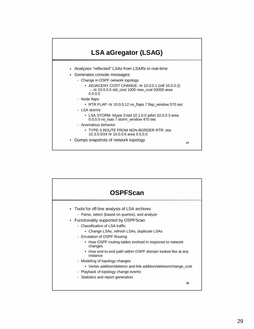
LSA aGregator (LSAG)

� Analyzes “reflected” LSAs from LSARs in real-time� Generates console messages:

- Change in OSPF network topology• ADJACENY COST CHANGE: rtr 10.0.0.1 (intf 10.0.0.2)

→ rtr 10.0.0.5 old_cost 1000 new_cost 50000 area 0.0.0.0

- Node flaps• RTR FLAP: rtr 10.0.0.12 no_flaps 7 flap_window 570 sec

- LSA storms• LSA STORM: lstype 3 lsid 10.1.0.0 advrt 10.0.0.3 area

0.0.0.0 no_lsas 7 storm_window 470 sec

- Anomalous behavior• TYPE-3 ROUTE FROM NON-BORDER RTR: ntw

10.3.0.0/24 rtr 10.0.0.6 area 0.0.0.0� Dumps snapshots of network topology

58

OSPFScan

� Tools for off-line analysis of LSA archives- Parse, select (based on queries), and analyze

� Functionality supported by OSPFScan- Classification of LSA traffic

• Change LSAs, refresh LSAs, duplicate LSAs- Emulation of OSPF Routing

• How OSPF routing tables evolved in response to network changes

• How end-to-end path within OSPF domain looked like at any instance

- Modeling of topology changes• Vertex addition/deletion and link addition/deletion/change_cost

- Playback of topology change events- Statistics and report generation

30

59

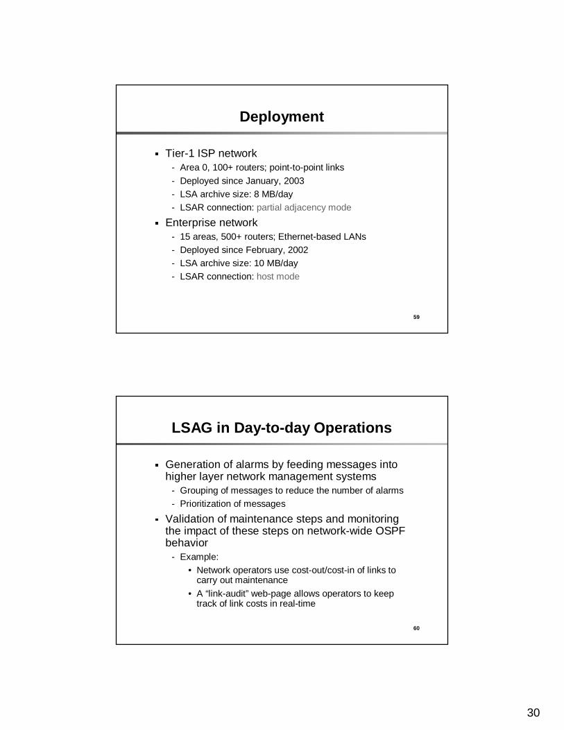
Deployment

� Tier-1 ISP network- Area 0, 100+ routers; point-to-point links

- Deployed since January, 2003- LSA archive size: 8 MB/day- LSAR connection: partial adjacency mode

� Enterprise network- 15 areas, 500+ routers; Ethernet-based LANs- Deployed since February, 2002- LSA archive size: 10 MB/day- LSAR connection: host mode

60

LSAG in Day-to-day Operations

� Generation of alarms by feeding messages into higher layer network management systems

- Grouping of messages to reduce the number of alarms- Prioritization of messages

� Validation of maintenance steps and monitoring the impact of these steps on network-wide OSPF behavior

- Example:• Network operators use cost-out/cost-in of links to

carry out maintenance

• A “link-audit” web-page allows operators to keep track of link costs in real-time

31

61

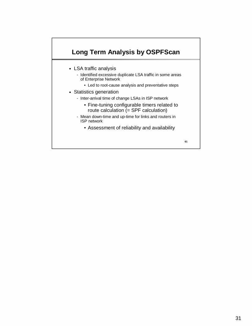
Long Term Analysis by OSPFScan

� LSA traffic analysis- Identified excessive duplicate LSA traffic in some areas

of Enterprise Network

• Led to root-cause analysis and preventative steps� Statistics generation

- Inter-arrival time of change LSAs in ISP network

• Fine-tuning configurable timers related to route calculation (= SPF calculation)

- Mean down-time and up-time for links and routers in ISP network

• Assessment of reliability and availability