CS 2750: Machine Learning Probability Review

Prof. Adriana KovashkaUniversity of Pittsburgh

February 29, 2016

Plan for today and next two classes

• Probability review• Density estimation• Naïve Bayes and Bayesian Belief Networks

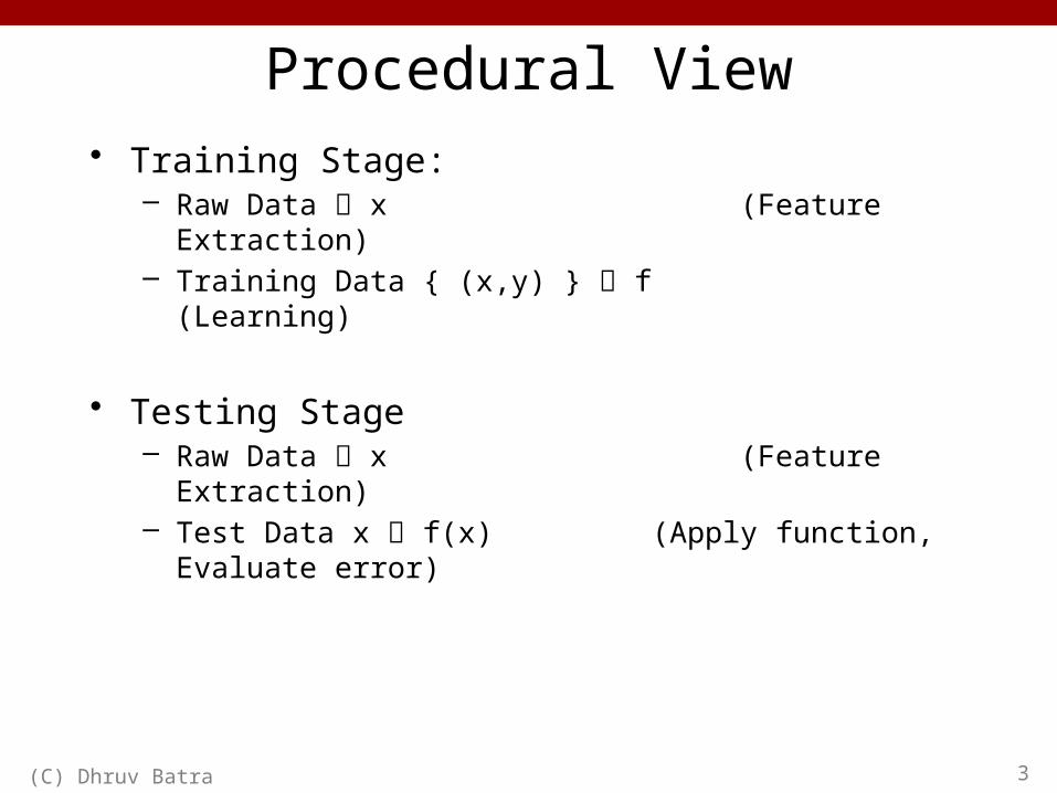
Procedural View• Training Stage:

– Raw Data x (Feature Extraction)– Training Data { (x,y) } f (Learning)

• Testing Stage– Raw Data x (Feature Extraction)– Test Data x f(x) (Apply function, Evaluate error)

(C) Dhruv Batra 3

Statistical Estimation View• Probabilities to rescue:

– x and y are random variables – D = (x1,y1), (x2,y2), …, (xN,yN) ~ P(X,Y)

• IID: Independent Identically Distributed– Both training & testing data sampled IID from P(X,Y)– Learn on training set– Have some hope of generalizing to test set

(C) Dhruv Batra 4

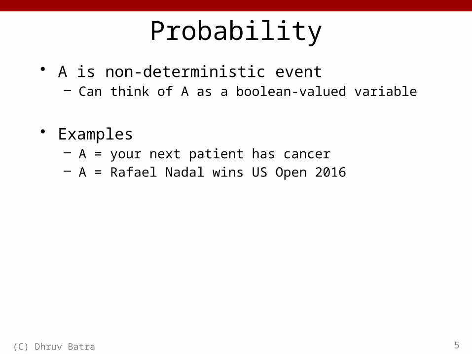
Probability• A is non-deterministic event

– Can think of A as a boolean-valued variable

• Examples– A = your next patient has cancer– A = Rafael Nadal wins US Open 2016

(C) Dhruv Batra 5

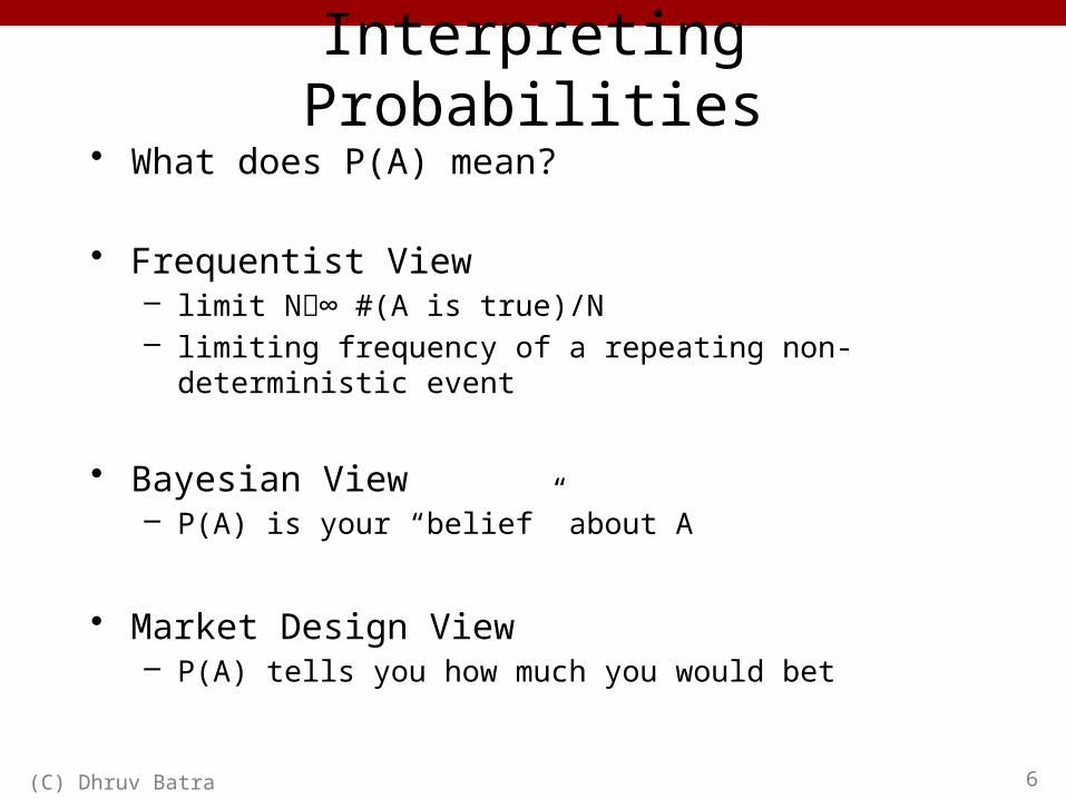
Interpreting Probabilities• What does P(A) mean?

• Frequentist View– limit N∞ #(A is true)/N– limiting frequency of a repeating non-deterministic event

• Bayesian View– P(A) is your “belief” about A

• Market Design View– P(A) tells you how much you would bet

(C) Dhruv Batra 6

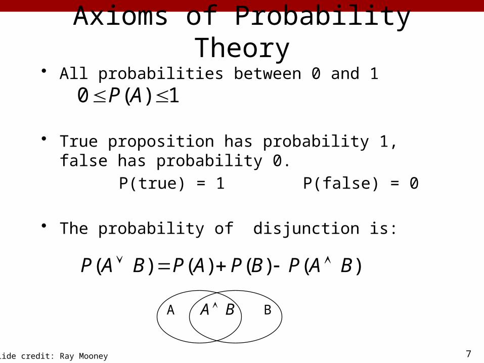
Axioms of Probability Theory• All probabilities between 0 and 1

• True proposition has probability 1, false has probability 0.

P(true) = 1 P(false) = 0

• The probability of disjunction is:

7

1)(0 AP

)()()()( BAPBPAPBAP

A BBA

Slide credit: Ray Mooney

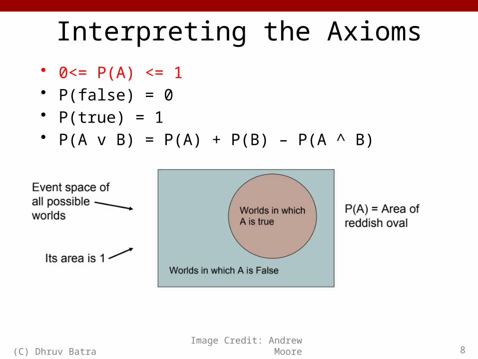
Interpreting the Axioms• 0<= P(A) <= 1• P(false) = 0• P(true) = 1• P(A v B) = P(A) + P(B) – P(A ^ B)

(C) Dhruv Batra 8Image Credit: Andrew Moore

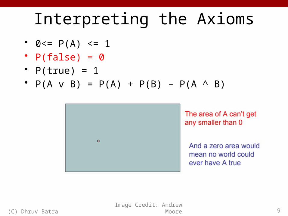
Interpreting the Axioms• 0<= P(A) <= 1• P(false) = 0• P(true) = 1• P(A v B) = P(A) + P(B) – P(A ^ B)

(C) Dhruv Batra 9Image Credit: Andrew Moore

Interpreting the Axioms• 0<= P(A) <= 1• P(false) = 0• P(true) = 1• P(A v B) = P(A) + P(B) – P(A ^ B)

(C) Dhruv Batra 10Image Credit: Andrew Moore

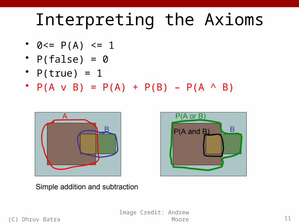
Interpreting the Axioms• 0<= P(A) <= 1• P(false) = 0• P(true) = 1• P(A v B) = P(A) + P(B) – P(A ^ B)

(C) Dhruv Batra 11Image Credit: Andrew Moore

Joint Distribution• The joint probability distribution for a set of random variables, X1,

…,Xn gives the probability of every combination of values (an n-dimensional array with vn values if all variables are discrete with v values, all vn values must sum to 1): P(X1,…,Xn)

• The probability of all possible conjunctions (assignments of values to some subset of variables) can be calculated by summing the appropriate subset of values from the joint distribution.

• Therefore, all conditional probabilities can also be calculated.

12

circle squarered 0.20 0.02blue 0.02 0.01

circle squarered 0.05 0.30blue 0.20 0.20

positive negative

25.005.020.0)( circleredP

80.025.020.0

)()()|(

circleredP

circleredpositivePcircleredpositiveP

57.03.005.002.020.0)( redP

Slide credit: Ray Mooney

Marginal Distributions

(C) Dhruv Batra Slide Credit: Erik Suddherth 13

Sum rule

y

z

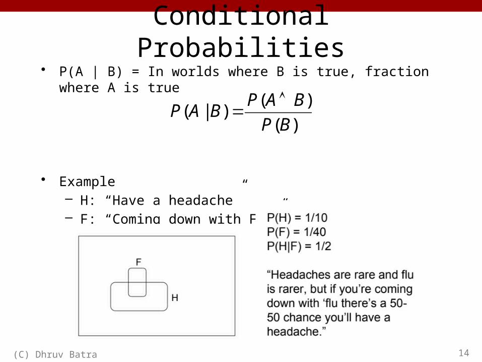
Conditional Probabilities• P(A | B) = In worlds where B is true, fraction where A is true

• Example– H: “Have a headache”– F: “Coming down with Flu”

(C) Dhruv Batra 14

)()()|(

BPBAPBAP

Conditional Probabilities• P(Y=y | X=x)

• What do you believe about Y=y, if I tell you X=x?

• P(Rafael Nadal wins US Open 2016)?

• What if I tell you:– He has won the US Open twice– Novak Djokovic is ranked 1; just won Australian Open

(C) Dhruv Batra 15

Conditional Distributions

(C) Dhruv Batra Slide Credit: Erik Sudderth 16

Product rule

Conditional Probabilities

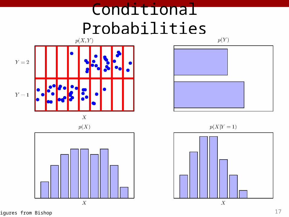
17Figures from Bishop

Chain rule• Generalized product rule:

• Example:

18Equations from Wikipedia

Independence• A and B are independent iff:

• Therefore, if A and B are independent:

19

)()|( APBAP

)()|( BPABP

)()(

)()|( APBP

BAPBAP

)()()( BPAPBAP

These two constraints are logically equivalent

Slide credit: Ray Mooney

• Marginal: P satisfies (X Y) if and only if– P(X=x,Y=y) = P(X=x) P(Y=y), xVal(X), yVal(Y)

• Conditional: P satisfies (X Y | Z) if and only if– P(X,Y|Z) = P(X|Z) P(Y|Z), xVal(X), yVal(Y), zVal(Z)

Independence

(C) Dhruv Batra 20

Independent Random Variables

(C) Dhruv Batra Slide Credit: Erik Sudderth 21

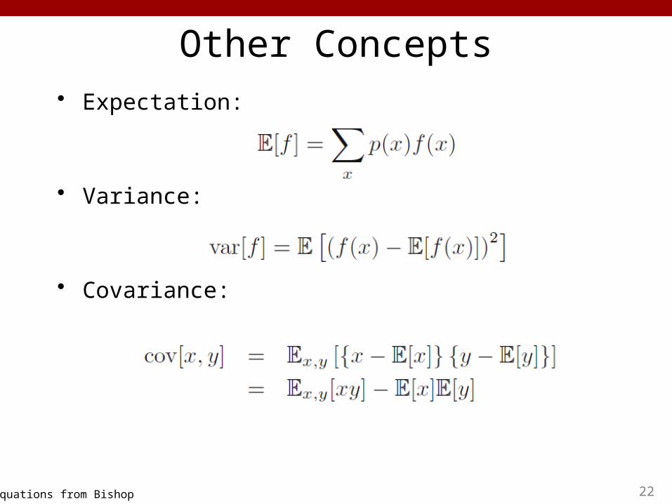
Other Concepts• Expectation:

• Variance:

• Covariance:

22Equations from Bishop

Entropy

(C) Dhruv Batra 24Slide Credit: Sam Roweis

KL-Divergence / Relative Entropy

(C) Dhruv Batra 25Slide Credit: Sam Roweis

26

Bayes Theorem

Simple proof from definition of conditional probability:

)()()|()|(

EPHPHEPEHP

)()()|(

EPEHPEHP

)()()|(

HPEHPHEP

)()|()()|()( EPEHPHPHEPEHP

QED:

(Def. cond. prob.)

(Def. cond. prob.)

)()()|()|(

EPHPHEPEHP

Adapted from Ray Mooney

27

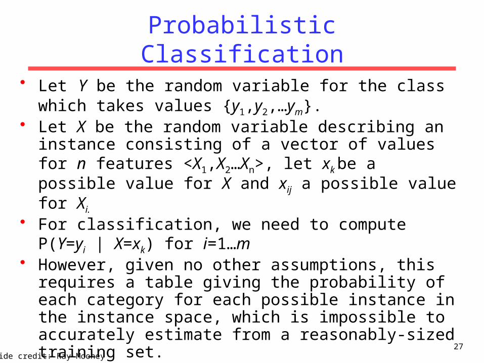
Probabilistic Classification

• Let Y be the random variable for the class which takes values {y1,y2,…ym}.

• Let X be the random variable describing an instance consisting of a vector of values for n features <X1,X2…Xn>, let xk be a possible value for X and xij a possible value for Xi.

• For classification, we need to compute P(Y=yi | X=xk) for i=1…m• However, given no other assumptions, this requires a table

giving the probability of each category for each possible instance in the instance space, which is impossible to accurately estimate from a reasonably-sized training set.– Assuming Y and all Xi are binary, we need 2n entries to specify

P(Y=pos | X=xk) for each of the 2n possible xk’s since

P(Y=neg | X=xk) = 1 – P(Y=pos | X=xk) – Compared to 2n+1 – 1 entries for the joint distribution P(Y,X1,X2…Xn)

Slide credit: Ray Mooney

28

Bayesian Categorization

• Determine category of xk by determining for each yi

• P(X=xk) can be determined since categories are complete and disjoint.

)()|()()|(

k

ikiki xXP

yYxXPyYPxXyYP

m

i k

ikim

iki xXP

yYxXPyYPxXyYP11

1)(

)|()()|(

m

iikik yYxXPyYPxXP

1

)|()()(

Adapted from Ray Mooney

posterior

prior likelihood

29

Bayesian Categorization (cont.)

• Need to know:– Priors: P(Y=yi) – Conditionals (likelihood): P(X=xk | Y=yi)

• P(Y=yi) are easily estimated from data. – If ni of the examples in D are in yi then P(Y=yi) = ni / |D|

• Too many possible instances (e.g. 2n for binary features) to estimate all P(X=xk | Y=yi).

• Need to make some sort of independence assumptions about the features to make learning tractable (more details later).

Adapted from Ray Mooney

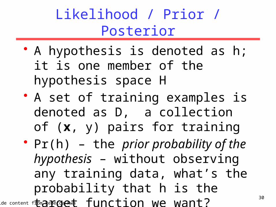
Likelihood / Prior / Posterior

• A hypothesis is denoted as h; it is one member of the hypothesis space H

• A set of training examples is denoted as D, a collection of (x, y) pairs for training

• Pr(h) – the prior probability of the hypothesis – without observing any training data, what’s the probability that h is the target function we want?

30Slide content from Rebecca Hwa

Likelihood / Prior / Posterior

• Pr(D) – the prior probability of the observed data – chance of getting the particular set of training examples D

• Pr(h|D) – the posterior probability of h – what is the probability that h is the target given that we’ve observed D?

• Pr(D|h) –the probability of getting D if h were true (a.k.a. likelihood of the data)

• Pr(h|D) = Pr(D|h)Pr(h)/Pr(D)31

Slide content from Rebecca Hwa

MAP vs MLE Estimation

• Maximum-a-posteriori (MAP) estimation:– hMAP = argmaxh Pr(h|D)

= argmaxh Pr(D|h)Pr(h)/Pr(D) = argmaxh Pr(D|h)Pr(h)

• Maximum likelihood estimation (MLE):– hML = argmax Pr(D|h)

32Slide content from Rebecca Hwa