cs 363 robotics, spring 2013 - colby college · cs363: mobile robotics lecture notes 2 robot...

CS363: Mobile Robotics Lecture Notes

CS 363 Robotics, Spring 2013

Dr. Bruce A. MaxwellDepartment of Computer Science

Colby College

Course Description

Robotics addresses the problems of controlling and motivating mechanical devices to act intelligently indynamic, unpredictable environments. Major topics will include: navigation and control, mapping and lo-calization, robot perception using vision and sonar, kinematics and inverse kinematics, and robot simulationenvironments. To demonstrate these concepts we will be using medium sized mobile robots capable of func-tioning in human environments. Lab and assignments will focus on programming robots to execute tasks,explore, and interact with their environment.

Prerequisites: CS 251 or permission of instructor.

Desired Course Outcomes

A. Students understand and can implement fundamental algorithms for robot control and navigation.

B. Students understand and can make use of a variety of sensors to enable autonomous robot behaviors.

C. Students understand the concept of state estimation applied to sensing, localization, and mapping.

D. Students work in a group to design software for controlling a robot.

E. Students present methods, algorithms, results, and designs in an organized and competently writtenmanner.

F. Students write, organize, and manage a large software project.

This material is copyrighted. Individuals are free to use this material for their own educational, non-commercial purposes. Distribution or copying of this material for commercial or for-prot purposes with-out the prior written consent of the copyright owner is a violation of copyright and subject to fines andpenalties.

c�2013 Bruce A. Maxwell 1 May 9, 2013


1 Robotics

What is a robot? Rod Brooks‘ definition:

• Situated: The robot has to live in a rich sensory environment and be capable of sensing the richness.

• Enabled: The robot has to be able to modify its environment or it is only an observer.

• Motivated: The robot has to be motivated to interact and modify its environment or it is a power tool.

1.1 A Brief History of Robotics

• 1206: Al-Jazari created the first programmable humanoid robot, a boat with four musicians that couldbe programmed to play different rhythms.

• 1868: Zadock Dederick designs and builds the first Steam Man, connected to a wagon.

• 1890: Nicola Tesla designs and builds radio-controlled robots, including an underwater robot.

• 1893: Georges Moore designs and builds a Steam Man, a biped which could walk at 5mph.

• 1940’s: Norbert Weiner designs the cybernetic AA gun, which uses radar to sense enemy planes.

• 1940’s: Scientists in Germany design the V1 and V2 rockets, which were arguably the first au-tonomous robots.

• 1950: W. Grey Walter designs and builds an autonomous turtle with sensors (eyes, ears, and feelers)and computational ability. The turtle could find its own recharging hutch and avoid obstacles.

• 1961: Unimate starts working on the GM assembly line.

• 1966-72: Development of SRI Shakey, the Stanford Cart, and the CMU Rover, autonomous robotswith vision and sensing.

• 1979: Robotics Institute founded at CMU by Raj Reddy

• 1981: Direct Drive arm built by Takeo Kanade

• 1994: Dante successfully samples gasses from within a volcano

• 1995: Navlab 2 drives 98% of the way across America.

• 1997: Home-vacuum event at the AAAI Robot competition (not a great showing)

• 1997: Sojourner navigates around Mars for 83 days (expected to last 7)

• 2002: Roomba goes on sale and becomes the first commercial robot to sell over a million entities.

• 2004: Spirit and Opportunity land on Mars. Opportunity is still going in 2013

• 2005: 5 teams complete the off-road DARPA grand challenge, a 200 mile are across the desert

• 2007: DARPA Urban Challenge won by ”Boss” of Tartan Racing

• 2011: Robonaut 2 delivered to the International Space Station

• 2012: Over 3500 PackBots in use by the military



2 Robot Designs

Robots come in many configurations and designs. All robots can move (or they wouldn’t be enabled), butthere are many different mechanisms for movement. Before we can write algorithms for making robotsmove, we have to understand how they can move and how that movement is parameterized.

• Walking (legs)

• Rolling (wheel or wheels)

• Slithering (undulation)

• Hopping

• Flying

• Swimming

While this course will focus on wheeled robots, the algorithms and methods we are learning are applicableto any robotic system that needs to sense its environment and take action.

Robot configurations are different than natural configurations in most cases. Machines do not yet matchnature in torque, response time, energy storage, or conversion efficiency at the same scales as biologicalsystems.

Machines do have actively powered rotational joints, however, which biological systems do not (biologicalsystems use passive joints with active muscles that contract or relax to cause the joint to move).

Key issues in locomotion:

• Stability:– Number and geometry of contact points– Center of gravity– Dynamic stability– Inclination of terrain– Potential external forces

• Characteristics of contact– Contact point/path size and shape– Angle of contact– Friction

• Type of environment– Structure– Medium

2.1 Legged Robots

Legged robots offer many advantages over wheel robots. Obstacles to rolling motion are not necessarilyobstacles to legged motion.

• Ground clearance is generally higher

• Local gradient of the terrain is irrelevant if the feet can find purchase

• A robot with flexible legs can manipulate the environment (everything is an arm)

Legged robots are not as common, however, because they require more power than an equivalently sizedwheeled robot, and generally have issues with weight and mechanical complexity. Newer motors and morecompact batteries, however, have made legged robots more realistic within the past five years.



• Legs need more than one degree of freedom (at least 2, and 3 is nice)

• Legs must be strong enough to support part of the robot’s weight

• Maneuverability requires many legs (or powered flexible joints) to produce forces in the directionrequired for a given maneuver (think spiders)

Legged robot configurations:

• Six legs plus: statically stable walking is possible. Hold three steady, move the other three.

• Four legs: statically stable walking is possible, and dynamically stable walking is possible with anactive control system.

• Two legs: statically stable walking is possible, and dynamically stable walking is possible with anactive control system.

• One leg: statically unstable configuration and requires a sophisticated control system.

If each leg can only lift, release, or hold, the number of possible events for a machine with k legs is:

N = (2k � 1)! (1)

For example, a two legged robot can lift either leg (2 events), release either leg (2 events), lift both legs,or release both legs. A six-legged robot has over 39 million possible choices at any given time step. Thisis one reason why learning methods have been most successful at learning gaits for robots like the SonyAibo, which has a multiple degrees of freedom in each leg and a range of velocities and angles it can movethrough.

2.2 Wheeled Robots

The advantage of wheeled robots is low power, low complexity, and higher speeds.

• Variety of configurations

• Efficient designs

• Good maneuverability

• Fast

The disadvantage is functionality in non-smooth terrain (non-zero local gradients)

Wheels

• Standard wheel: rotation around the wheel axle and around the contact point

• Castor wheel: rotation around the wheel axle and an offset steering joint

• Swedish wheel: rotation around the wheel axle, contact point, and rollers

• Ball or spherical wheel: rotation around the center of the sphere (difficult to implement)

Regardless of wheel selection, for anything but smooth ground you need a suspension system to keep thewheels in contact with the ground at all times. Sometimes the suspension system is as simple as an inflatabletire (effectively a tight spring), but sometimes it is much more complex.



Question: can you have only two wheels and not fall over?

Wheel geometries (Table 2.1 of Siegwart and Nourbakhsh)

• Bicycle/motorcycle

• Two-wheel differential drive w/COM below wheel axle - Cye robot

• Two-wheel differential drive with castor - Nomad/Magellan

• Two powered traction wheels, one steered front wheel - Piaggio minitrucks

• Two unpowered wheels, one steered, powered front wheel - Neptune (CMU)

• Three motorized Swedish wheels - Palm Pilot robot kit

• Three synchronously motorized & steered wheels (“Synchro drive”) - B21r

• Ackerman wheel configuration, front and rear-wheel drive - automobiles

• Four fixed wheels using skid steering - ATRV

• Four steered and motorized wheels - Hyperion, construction vehicles

• Four Swedish wheels - Uranus (CMU)

• Two-wheel differential drive with two castors - Khepera

• Four motorized and steered castor wheels - Nomad XR4000

Maneuverability v. Controllability: the maneuverability, or flexibility of a robot is generally inverselyrelated to its controllability. The most difficult robots to control are the swedish wheels and the steeredcastors, yet they also offer true holonomic ability (they can move in any direction instantaneously). TheAckerman steering system (think cars) is one of the least maneuverable, yet the control system for it is quitesimple and the arrangement is very stable. Differential drive systems balance the two characteristics.

3 Sensing

3.1 Proximity sensors

Contact sensors

• Push-button: put a plate over a push-button switch, useful as a fail-safe to tell the robot to stopimmediately. On the Roomba, they play a central role in obstacle avoidance and navigation.

• Contact surfaces: capacitive or optical screens that sense touch (e.g. iPhone). Handed robots oftenhave contact sensors on the finger/gripper surfaces.

• Big red stop buttons: a critical safety feature, especially for big robots. They generally break powerto the motors. These have been used on systems such as robotic combines and placed in strategiclocations to they can be triggered by a person’s head if the robot has pinned their arms against a wall(Carl Wellington, CMU Graduate)

• Feelers/Antennae: Put a wire on a contact switch. If the wire brushes something, the switch is closed.These can be very useful for avoiding feet or wall-following. It is also possible to put strain gagesor flex sensors on an antenna, which give a continuous range of values depending upon the degree of



contact. These have been used to simulate a cockroach moving along a wall using only its feeler as asensor (Lee et. al, “Templates and Anchors for Antenna-Based Wall Following in Cockroaches andRobots”, IEEE Trans. on Robotics, 2008).

IR sensors

• The old versions of IR sensors used a focused IR LED to send out a beam of light and a simple IRphotosensor to detect the intensity of the reflection. The output told you how much light was beingreflected, but that was not always correlated with distance. Ambient light, or dark objects could causebiases in the range values returned.

• The new versions of IR sensors, the Sharp IR Rangers, use a linear strip of detectors and estimaterange using triangulation rather that reflected intensity. They are available in a variety of distancesfrom 0.3m to 5.5m, with different models have different minimum and maximum ranges. Some IRsensors provide a Boolean output, others a continuous output

• Both versions of the IR sensors have a fairly tight focus, especially compared to a sonar.

• The response of the IR sensors (raw voltages) are not linear with distance, and require a lookup-table.The noise profile is not bad (approximately Gaussian) once the data is linearized.

Sonar sensors

• Uses a piezoelectric material to send out a pulse of sound. The same material detects the reflection ofthe pulse and measures the time of flight. Sonars are useful out to 3-4m, but not as much use within0.25m because there has to be sufficient time between sending the pulse and sensing its return for thevibrations to damp down.

• Senses within a fairly broad cone, and anything within the cone generates a signal.

• The major difficulty with sonars is reflection–at oblique angles the sound doesn’t come back. Simplenoise is not as much of a problem as noise due too reflections, which produce the equivalent of noobstacle. The noise profile is approximately Gaussian with no reflection, but reflection adds a shotnoise component where some readings are extreme.

• Sonars are much more effective in underwater environments, and they are a primary method of map-ping and localizing for marine robots.

Laser sensors

• Laser + camera - scan a laser across a scene and use a camera with a filter tuned to the laser’s frequencyto track where the laser reflects and use triangulation to estimate distance. The camera can be 2D or3D, and must be calibrated with respect to the laser’s position. Maintaining calibration can be difficulton moving vehicles, but this is generally the cheapest option for creating a simple laser scanner andcan be implemented with a line laser and cheap camera.

• Laser range finder: 2D scan - time of flight to estimate distance using a pulsed signal. Time of flightis generally measured using the phase change of the signal.

• Laser range finder: 2D scan + PT mount - put a 2D scanner on a pan tilt mount and swing it around.Provides 3D information.

• Laser range finder: 3D scan - full 3D scan - time of flight using a 3D array. Enables 3D informationwith temporal coherence.



3.2 Proprioception

• Accelerometers - measure accelerations by using the phase response of lasers on a chip. Modernaccelerometers are small and sufficiently accurate to permit double integration to estimate distancetraveled.

• Gyroscopes - measure angular rotation, generally in three axes. Modern gyroscopes are laser-basedrather than physical mechanisms.

• Compass - measures orientation relative to the local magnetic field. Electronic compasses have nomoving parts and use the Hall effect to measure the local field.

• GPS - uses the Global Positioning Satellites to estimate 3D position and orientation. Modern GPSdevices have accuracies of centimeters, but still may have issues with jumps from time to time.

• Computational load - robot knows when it is running into computational limits.

• Internal temperature sensors - used to manage power consumption or recognize dangerous situations.

• Battery life - robot knows when it needs to recharge itself.

3.3 Environmental Sensors

• Motion sensors - designed to respond to motion in the sensor field. Motion sensors can be IR sensorsor temperature sensors looking for fluctuations in a small field of sensors.

• Temperature sensors - IR sensors that return a signal responsive to absolute temperature levels. Theseare used often in robotic USAR situations when looking for victims, who may be invisible to regularvisual sensors and may not be moving.

• CO2 sensors - measure the concentration of CO2 gas, also commonly used in robotic USAR situations.

• Chemical sensors - there are a variety of special-purpose chemical sensors that are able to detect smallconcentrations of a particular chemical. Some researchers, inspired in part by ants, have looked intousing them for laying down trails or assisting in searching an area by marking what locations havealready been searched. Chemical sensors are a primary sensor for land mine detection robots.

3.4 Cameras

• Sensor technology

– CCD - Charge-Coupled Device [CCD] cameras use a process that captures photons/electrons insilicon wells. The charge can be moved from well to well in order to read it off as a row. CCDcameras used to have lower noise and higher dynamic range because of their slightly larger wellsizes.

– CMOS - Complementary Metal Oxide Semiconductor [CMOS] cameras use a standard chipmanufacturing process and generally integrate the electronics for each pixel next to the sensorwell. The easy integration of electronics and sensor enables manufacturers to do some interestingon-chip processing.



– Greyscale - greyscale cameras have no filters over the sensor except possibly an infrared cutofffilter to increase the camera’s sensitivity to visible light. Silicon is sensitive to IR wavelengths,so without the IR cutoff filter the camera tends to be saturated with the IR signal in naturallight. It also possible, however, to remove the IR cutoff filter and block visible light, producinga mid-quality IR camera.

– Color - single CCD/CMOS color cameras use an array of red, green and blue [RGB] filters laidout in a grid called a Bayer pattern. Each set of four pixels has one red, one blue, and two greensensors. Human vision is most sensitive to wavelengths in the green channel, which is why theyuse a second green sensor to get a higher signal to noise ratio. Either the camera or softwareon the camera interpolates the local information in each color channel to produce an RGB valueat each pixel. Two-thirds of the data in an image from a single sensor color camera, therefore,is a result of interpolation, not measurement. For this reason, greyscale cameras are often usedwhere dynamic range, low noise, or low-light sensitivity is critical. A greyscale camera devotesfour times as much pixel area to each measurement compared to a color camera, and integratesphotons from across the visible spectrum. Note that in higher end cameras, the RAW formatdata holds only the actual sensor measurements, permitting customized software to implementthe interpolation–or not–as desired.

– Multi-sensor - some cameras use three sensors instead of one, using a prism to split the incominglight into three parts and putting a different color filter over each sensor. A 3 sensor color cameragenerally has lower noise that a single CCD camera, even after splitting the incoming light,because each sensor is a greyscale sensor and has a much larger surface area than the pixels ona color camera.



• Image capture methods

– Line scan - a line scan camera is a single linear array of sensors. Line scan cameras are oftenused in industrial processes on assembly lines for products like paper. They have also been usedfor high resolution aerial mapping. The benefit of a line scan camera is the data rate. Since ithas only a single row of pixels, you can read out the pixels at a high frame rate and transfer thedata easily.

– Frame scan - a frame scan camera has a 2D pixel array with the odd rows assigned to frame 0and the even rows assigned to frame 1. The camera reads out the frames in alternating order andpacks them together in a single image. The scene, therefore, is imaged at 60Hz at half resolutionor 30Hz at full resolution. One result of reading the frames at different times is that a movingobject can appear in two places in the scene. Frame scan chips are rarely used now, especiallywith the advent of CMOS camera sensors. Some older stereo camera systems would take ahalf-height image from each camera, capture simultaneously, and put them together as the twoframes of a single image.

– Progressive scan - a progressive scan camera grabs the entire frame simultaneously. Most currentcamera systems are progressive scan. It is possible to get much higher frame rates from cameras,but most cameras have a frame rate of no more than 30Hz.

• Sensor geometries

– Single camera - most camera systems are a single camera, possibly on a pan-tilt mount and withzoom capabilities.

– Binary stereo - binary stereo requires two synchronized cameras in a fixed relative orientation.With proper calibration and software, binary stereo cameras can provide both reflectance anddistance information. Depending on the scene, the distance information may be sparse or dense.Scenes with little texture or variation are difficult for stereo algorithms to analyze.

– Multi-view stereo - binary stereo provides only two views of a scene. Adding more camerasprovides more robustness to depth estimation, and there are simple algorithms for combiningthe information from many cameras. A common configuration for multiple cameras is an L.

– Panoramic cameras - Many robot systems have used panoramic cameras, which combine a regu-lar camera with a parabolic mirror. The camera points straight up at the parabolic mirror, whichreflects information from 360

�. A single image, therefore, contains an entire panoramic image.Objects closer to the robot are closer to the center of the image, while the horizon sits on a circleon the outer edge of the image. Given the geometry is known, it is possible to re-sample thecircular image into a more traditional rectangular image.



4 Motion, Kinematics, and Control

Representation of robot state: where is the robot in the world (pick an origin)?

• Linear robot: S = (x)

• Planar mobile robot: S = (x, y, ✓)

• Mobile robot in natural terrain: S = (x, y, z, ✓,�, �)

• Aerial/underwater robot: S = (x, y, z, ✓,�, �)

• Jointed mobile robot (e.g. humanoid) on a plane: S = (x, y, ✓, ~⇥)

Coordinate systems

• World - arbitrary definition of the origin, generally selected to be convenient (e.g. corner of a room).

• Robot - attached to the robot, generally defined as X forward, Y left, and Z up, specified relative tothe world coordinate system.

• Camera - attached to the camera, specified relative to the robot.

• Laser - attached to the laser, specified relative to the robot

• Sonar - attached to each sonar sensor, specified relative to the robot

• Manipulator - attached to the end effector of the manipulator, transformations link each joint of themanipulator in a chain to the robot coordinate system

4.1 Transformations

If we describe a robot’s pose as a vector, then we can describe both translations and rotations using matrices.Consider, for example, an oriented robot moving on a plane. The position of the robot is given by twoparameters (x, y) and the pose of the robot is given by ✓.

A translation by (tx

, ty

) is defined by the matrix (2).

T (tx

, ty

) =

2

4

1 0 tx

0 1 ty

0 0 1

3

5 (2)

If we multiply the robot’s pose by the translation matrix, the robot’s pose changes by adding tx

to the xposition and t

y

to y position.

2

4

x0

+ tx

y0

+ ty

✓

3

5

=

2

4

1 0 tx

0 1 ty

0 0 1

3

5

2

4

x0

y0

✓

3

5 (3)

A rotation by an angle ✓ can also be represented as a matrix as in (4).

RZ

(✓) =

2

4

cos ✓ � sin ✓ 0

sin ✓ cos ✓ 0

0 0 1

3

5 (4)



Rotation matrices are useful for relating the robot’s local coordination system, which moves as the robotturns, to the global coordinate system, which is fixed. For a planar robot, the robot‘s local coordinate systemis defined by its current orientation, ✓. Motion in the robot‘s local coordinate system can be described inthe global coordinate system using a simple rotation matrix to transform the motion from a local velocity(x

l

, yl

, ˙✓) to a global velocity (xg

, yg

, ˙✓). The robot’s current orientation ✓ defines the transformation. To de-scribe local coordinates in a global coordinate system, we need to rotate by the rotation matrix R

Z

(✓).

2

4

xg

yg

˙✓

3

5

= RZ

(✓)

2

4

xl

yl

˙✓

3

5

=

2

4


sin ✓ cos ✓ 0

0 0 1

3

5

2

4

xl

yl

˙✓

3

5

(5)

Using (5) we know how to update the robot’s global position given its current velocity and heading. If therobot currently has a pose defined by ✓, then motion in the local coordinate system, specified by (x

l

, yl

) overa small time step �t will change the robot‘s global position (x

g

, yg

) by the amount �t(xg

, yg

).

Note that Siegwart and Nourbakhsh give a different definition of a rotation matrix that is the transpose ofthe one above. For rotation according to the right-hand rule, the proper matrix has the negative sine term inthe first row, not the second. Consider, for example, rotating the vector

⇥

1 1 1

⇤

t by ⇡/2, which shouldresult in

⇥

�1 1 1

⇤

t.

2

4

xf

yf

zf

3

5

= R(⇡/2)

2

4

1

1

1

3

5

=

2

4

cos⇡/2 � sin⇡/2 0

sin⇡/2 cos⇡/2 0

0 0 1

3

5

2

4

1

1

1

3

5

=

2

4

0 �1 0

1 0 0

0 0 1

3

5

2

4

1

1

1

3

5

=

2

4

�11

1

3

5

(6)

Transposing the rotation matrix would result in the vector⇥

1 �1 1

⇤

t, which is rotation according tothe left-hand rule.



4.2 Kinematics

Kinematics is the study of how physical systems can move. One way to view kinematics is, given a robot’spose, what are all the motions it can execute instantaneously. Another way to think about it is that the kine-matics of an object describe all the possible poses the object can take given a starting location. Kinematicscan be used to analyze both questions.

The movement, or current pose of any physical system can be described as a set of parameters. Eachparameter describes either rotational motion around an axis or linear motion along an axis. By combiningrotations and translations we can define all of the complex motions executable by a robot and estimate wherea robot will be after the motion.

All robots have a kinematic description. In some cases, such as a planar robot with swedish wheels, thekinematics are simple: the robot is able to move in any direction instantaneously. In other cases, such as ona car, the kinematics tell us the possible arcs along which the car can travel. In a plane with no obstacles,any robot capable of moving in two independent directions can achieve any configuration, although differentrobots have to follow different paths. In a plane with obstacles, that is not necessarily the case.

Kinematics are especially important in path planning; the kinematics define the possible actions available tothe planner.

4.2.1 Differential drive kinematics

Consider a differential drive robot with two standard wheels of radius r, each separately controllable. Thecenter of the robot, or the origin of the robot is the point P . Let the wheels each be a distance l from P . Theangular velocity (radians/s) of the two wheels is given by (�

1

,�2

). When a wheel completes a full turn–2⇡radians–then the wheel has traveled 2⇡r units. Therefore, it moves a distance r per radian of rotation andthe velocity of the wheel relative to the plane is given by r� for a rotational velocity of �.

The equation of motion of the central point P due to turning wheel A can be expressed as a rotation aboutthe location of wheel B. Likewise, motion due to turning wheel B can be expressed as a rotation about thelocation of wheel A. Motion by both wheels adds some degree of translation. If both wheels turn the sameamount, the robot’s orientation does not change. If the wheels turn equal, but opposite amounts, the robot’sposition does not change, but its orientation does.

One way to visualize the kinematics of a differential drive is to define the space of possible rotation centers.If both wheels are rotating in equal, but opposite directions the rotation center is the middle of the robot. Ifthe two wheels are turning simultaneously forward, the center of rotation is at infinity along the y-axis. Ifthey turn simultaneously backward, the center of rotation is at infinity along the negative y-axis. If the twowheels are moving differently, then the center of rotation lies somewhere on a line connecting the center ofthe robot and the points at ±1 along the y-axis.

The kinematic description of a wheeled robot’s position over time is complex to calculate because it dependsupon the relative motion of the two wheels over time. At every instant the robot is rotating around somelocation along the axis of rotation of the two wheels, but the instantaneous center of rotation depends uponthe relative speed of the two wheels and changes over time. Because the motion, and therefore the finalposition, of the robot depends upon the instantaneous center of rotation, the ordering in time of the wheelrotations is important.

A simple exercise demonstrates that the final position of the robot does depend upon the particular path



taken by the robot. Consider, for example, a sequence of operations where the robot first rotates the rightwheel so the point of contact follows a path of length d, then rotates the left wheel by the same amount. Thefirst rotation will move the origin of the robot along a circle of radius l around the left wheel contact. Thesecond rotation by the left wheel will rotate the robot around the new location of the right wheel. The endresult will be the robot shifting to the left and forward of its starting location. By contrast, executing therotations in the opposite order will shift the robot to the right and forward of its starting location. Executingthe motion of the wheels simultaneously would move the robot forward by a distance d.

We can obtain the new location of the robot after a single rotation by using the translation and rotationsmatrices to rotate the origin about the left wheel contact. To rotate the plane about an arbitrary point, we usea a three-step method:

1. Translate the center of rotation to the origin using T (�cx

,�cy

).

2. Rotate about the origin by ✓ using RZ

(✓).

3. Translate the center of rotation back to its original position using T (cx

, cy

).

Rc

(✓) = T (cx

, cy

)RZ

(✓)T (�cx

,�cy

)

=

2

4

1 0 cx

0 1 cy

0 0 1

3

5

2

4


sin ✓ cos ✓ 0

0 0 1

3

5

2

4

1 0 �cx

0 1 �cy

0 0 1

3

5

=

2

4

cos ✓ � sin ✓ cx

(1� cos ✓) + cy

sin ✓sin ✓ cos ✓ c

y

(1� cos ✓) + cx

sin ✓0 0 1

3

5

(7)

Therefore, if we multiply the origin (0, 0) by Rc

(✓) using a pivot point of (cx

, cy

) = (0, l), then we get thelocation of the robot after rotating the left wheel.

2

4

l sin ✓l(1� cos ✓)

1

3

5

=

2

4

cos ✓ � sin ✓ l sin ✓sin ✓ cos ✓ l(1� cos ✓)0 0 1

3

5

2

4

0

0

1

3

5 (8)

Given the location of the robot‘s origin after the motion of the right wheel, we can use the same process torotate about the right wheel as the left wheel rotates. However, the right wheel has moved from its originallocation, so the pivot point has changed. Therefore, the second rotation will move the robot in a circular arccentered on the new location of the right wheel. The end result will put the robot to the left and forward ofits original location.

Because of the path dependence of the motion of a differential drive a planar mobile robot, it is actuallyeasier to consider the relationship between wheel velocities and robot velocities than wheel position androbot position.

Instantaneous velocity by one wheel gives the robot’s origin a velocity along the x-axis (which points for-ward). As the wheels are equidistant from the robot‘s origin, the origin moves by half the velocity of thewheel. A wheel of radius r has a translational velocity along the ground that is equal to r�

i

, and the con-tributions of two wheels add together. Therefore, the translation of the robot along the x-axis is given by(9).

x =

r�1

2

+

r�2

2

(9)



Instantaneous velocity in the y-axis is impossible because a standard wheel rotates about the y-axis.

y = 0 (10)

To obtain the rotational velocity of the robot ˙✓, consider that rotation of one wheel will cause the robot’scenter to move in a circle of radius l, and the outer wheel in a circle of radius 2l. The robot will completea circle, which is a rotation of 2⇡ radians, in the time t it takes for the outer wheel to go a distance of ⇡4l.The distance traveled by the wheel given the wheel’s rotational velocity �

i

is given by (11).

d = tr�i

(11)

The time taken for the robot to traverse a complete circle is given by (12).

t =⇡4l

r�i

(12)

The angular velocity is given by 2⇡/t, which gives us the angular velocity due to a single wheel.

˙✓ =

r�i

2l(13)

The contributions of each wheel add together, but cause opposite rotations. The total instantaneous angularvelocity is given by (14).

˙✓ =

r�1

2l� r�

2

2l(14)

The above relationships exist in the robot‘s local coordinate system, so to transform them to the globalcoordinate system we need to multiply the local change by the inverse of the rotation matrix defined by therobot‘s current heading. The full model for a differential drive robot is given by (15).

2

4

xg

yg

˙✓

3

5

= R(✓)

2

4

r�12

+

r�22

0

r�12l

� r�22l

3

5 (15)

If we extract out the wheel velocities (joint velocities), then we can rewrite (15) as a relationship betweenthe wheel velocities and the global translational and rotational velocities of the robot.

2

4

xg

yg

˙✓

3

5

= R(✓)

2

4

r

2

r

2

0

0 0 1

r

2l

� r

2l

0

3

5

2

4

�1

�2

0

3

5 (16)

Note that (16) explicitly gives what’s called the Jacobian for the differential drive robot. The Jacobian definesthe relationship between the joint angular velocities and the robot state velocities. Note that the Jacobianis dependent upon the current robot configuration (✓) through the rotation matrix. Therefore, it must becomputed dynamically at every time step. By separating the process into two parts, however, only theinverse of the rotation matrix is required, and the inverse of a rotation matrix is simply its transpose.



Figure 1: Two joints connected by a rigid linkage

4.2.2 Joint Kinematics

For linkages that can be represented as a rigid bar connecting two joints, we can generate a generic matrixtransformation that applies equally well to linear and rotational joints. The transformation describes motionin one joint’s coordinate system with respect to the other. Such a representation is important for robotmanipulators, which are increasingly being used on mobile robot platforms for manipulation tasks.

Consider figure 1, which shows two joints connected by a rigid link.

• The motion of the joint is always defined to be around or along the local z-axis of the joint.

• The local x-axis of the joint always points towards the next joint.

• The angle between axis Zi�1

and Zi

is defined as ↵i�1

.

• The distance along axis Xi�1

between axis Zi�1

and Zi

is defined as ai�1

.

• The angle around axis Zi

between axis Xi�1

and Xi

is defined as ✓i

.

• The distance along axis Zi

between Xi�1

and Xi

is defined as di

.

The active motion of the ith joint is defined by either ✓i

or di

, while the linkage connecting joints i �1 and i is defined by ↵

i�1

and ai�1

. Using these definitions, we can define a transformation i�1

i

T thattransforms motion in frame of reference i into motion in frame of reference i� 1. The order or operation oftransformation matrices is right to left given a column vector and right multiplication.

i�1

i

T = RX

(↵i�1

)T (ai�1

, 0, 0)RZ

(✓i

)T (0, 0, di

) (17)

Recursive use of the kinematic relationship in (17) defines the position of the end effector at the last jointin the coordinate system of the first joint as a function of the joint parameters (✓

1

, . . . , ✓N

). The functionf(✓

1

, . . . , ✓N

) is defined a the forward kinematic equation, and it tells us the position of the last linkagegiven the joint angles. However, it does not tell us how the end effector will move if, for example, we wereto change a single joint angle ✓

i

. Different joint angles will cause different types of motion.



Example: Robonova arm

Figure 2: Diagram of Robonova arm joints

The Robonova arm has three joints, shown in figure 2: two at the shoulder and one at the elbow. We canorganize the parameters of the arm, as in table 1, showing ↵

i�1

, ai�1

, ✓i

, and di

for each joint. Note thatto get between the first and second joints, we have to insert a rigid joint to move the x-axis into the properorientation. The last transformation gives the frame of reference for the end effector.

Joint ↵i�1

ai�1

✓i

di

0 0 0 ✓0

0- ⇡/2 0 ⇡/2 01 a

0

0 ✓1

02 0 a

1

✓2

03 0 a

2

0 0

Table 1: Joint parameters for the robonova arm.

A complete joint transformation between two frames is given by (18).

i�1

i

T =

2

6

6

4

cos ✓i

� sin ✓i

0 ai�1

sin ✓i

cos↵i�1

cos ✓i

cos↵i�1

� sin↵i�1

� sin↵i�1

di

sin ✓i

sin↵i�1

cos ✓i

sin↵i�1

� cos↵i�1

� cos↵i�1

di

0 0 0 1

3

7

7

5

(18)

Plugging the values from the table into (18) gives us the each of the individual transformations from frameto frame. The multiplication of all of the frames gives us the complete transformation. The completetransformation matrix is an exact description of the end effector position given the joint angles. Note thatmost of the transformations are simple, as many of the parameters for each joint are zero.



4.2.3 Jacobian

In order to identify how the end effector will respond to a particular set of joint motions, or velocities, weneed to calculate the Jacobian, which is a matrix of partial derivatives of the kinematic equation for eachaxis with respect to each joint angle. Consider, for example, a planar robot where the position of the endeffector is defined by two functions f

x

(✓1

, . . . , ✓N

) and fy

(✓1

, . . . , ✓N

), which define its x and y positionsas a function of the joint angles.

The Jacobian of this system would be defined as in (19).

J(⇥) =

"

@f

x

(✓1,...,✓N

)

@✓1. . . @f

x

(✓1,...,✓N

)

@✓

N

@f

y

(✓1,...,✓N

)

@✓1. . . @f

y

(✓1,...,✓N

)

@✓

N

#

(19)

The utility of the Jacobian is that if we have a set of joint velocities ( ˙✓1

, . . . , ˙✓N

), then we can calculate theinstantaneous change, or the velocity of the end effector, which tells us how it moves in response to the jointangle velocities.

xy

�

= J(⇥)

2

4

˙✓1

. . .˙✓N

3

5

=

"

@f

x

(✓1,...,✓N

)

@✓1. . . @f

x

(✓1,...,✓N

)

@✓

N

@f

y

(✓1,...,✓N

)

@✓1. . . @f

y

(✓1,...,✓N

)

@✓

N

#

2

4

˙✓1

. . .˙✓N

3

5 (20)

Better yet, if we take the inverse of the Jacobian, J�1

(⇥), then we can identify the joint velocities necessaryto achieve a certain motion of the end effector.

2

4

˙✓1

. . .˙✓N

3

5

= J�1

(⇥)

xy

�

(21)

One of the uses for the Jacobian is identifying the sequence of joint angle velocities required to make anend effector follow a specific path. The technique is commonly used in robot manipulators. The difficultywith the method is that the forward kinematic equation is dependent upon the joint angles. Therefore, theJacobian, which is based on the derivatives of the forward kinematic equation, changes as the joint angleschange. In order to obtain the correct relationship between the joint angle and end-effector velocities, ateach time step the current Jacobian matrix must be calculated and inverted. While this is no longer acomputational issue given current processing power, the Jacobian is not guaranteed to be invertible, so careneeds to be taken to handle special cases.



4.3 Robot Control

There are many approaches to robot control, many of which are based on sophisticated mathematics. Thereare also very simple approaches that use straightforward rules designed by programmers. In general, themore you can model your robot‘s response to inputs and use those models to define control strategies, themore sophisticated and robust your robot‘s behavior will be.

There are also many levels of robot control. At a very low level you want something on your robot to belooking out for obstacles and responding appropriately, which may include stopping as quickly as possible.At a high level, you may want your robot to follow walls, explore a maze, wander, or track through a seriesof waypoints.

4.4 Basic Control Theory

Open loop control is when you control something, like a robot, without any feedback from internal orexternal sensors to indicate how well you have achieved your goal. Its like walking down a corridor withyour eyes close and hands behind your back: eventually you run into the wall. Using odometry to control arobot is insufficient over time, as errors in the position estimate grow without bound.

Feedback control uses internal or external sensing to determine the error between the actual and desiredstate of the device/robot. What to do at each instant of time is determined by the error and the controllaw. Most real systems are run as closed loop control systems, because otherwise small errors in motioneventually lead to big errors in position.

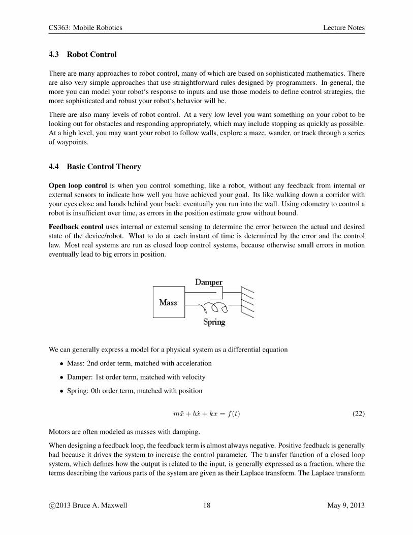
We can generally express a model for a physical system as a differential equation

• Mass: 2nd order term, matched with acceleration

• Damper: 1st order term, matched with velocity

• Spring: 0th order term, matched with position

mx+ bx+ kx = f(t) (22)

Motors are often modeled as masses with damping.

When designing a feedback loop, the feedback term is almost always negative. Positive feedback is generallybad because it drives the system to increase the control parameter. The transfer function of a closed loopsystem, which defines how the output is related to the input, is generally expressed as a fraction, where theterms describing the various parts of the system are given as their Laplace transform. The Laplace transform



(a) Open loop control (b) Closed loop control (c) Closed loop control

is a method of transforming differential equations from the time domain to the frequency domain, whichoften makes analysis simpler. A second order system, such as above, would be represented as in (23).

ms2 + bs+ k = F (s) (23)

Given the Laplace representation of the parts of the control systems, we can write the open and closed loopfeedback control as in (24) and (25), respectively.

C(s) = G(s)R(s) (24)

C(s) =F (s)G(s)

1 + F (s)G(s)H(s)R(s) (25)

(25) defines how the output C(s) is related to the input signal R(s).

• H(s) is the feedback function that is part of the control software.

• F(s) is a compensator function that is part of the control software.

• G(s) is the plant, or the robot’s mechanical system and is described as a differential equation.

As an example, H might be the identity (1), and F might be a simple constant (P), in which case the transferfunction looks like (26).

C(s) =PG(s)

1 + PG(s)R(s) (26)

It is possible, given an accurate description of the plant and the control system, to demonstrate the expectedbehavior of the system as a whole given the feedback and compensator functions. An analysis of the feed-back equations also shows us how different control parameters will affect the system. In general, for a givencriterion, we can optimize the system performance by adjusting the control system parameters and form.Common criteria for optimization include: time to achieve the goal, and the degree of overshoot. Overshootoccurs when the control system goes past the desired goal and has to come back to it from the other side. Asmall amount of overshoot is often permitted because it speeds up the system’s initial response to a controlsignal.

Without specific knowledge of the plant, it can be difficult to identify appropriate control systems. Ingeneral, though, if the plant is well-behaved, then there are some common approaches to control that provideacceptable performance given a small amount of experimentation.



4.4.1 Proportional control

The simplest control law is proportional control. Using proportional control, the control signal is propor-tional to the error between the desired and actual system outputs. A constant k

p

, determines the speed andcharacter of the system‘s response to a change in inputs.

In terms of the feedback loop diagram, Proportional control means setting F = kp

and H = 1.

There are four regimes, or behaviors, in the response of the system to a proportional control law. The fourregions are defined by the value of k

p

relative to the critical damping factor kc

and the unstable dampingfactor k

u

.

• kp

< kc

overdamped: the response is a smooth exponential curve to the desired output

• kp

= kc

critically damped the response is a smooth exponential curve to the desired output, and isas fast a response as possible without overshooting the desired output.

• kc

< kp

< ku

underdamped: the response will overshoot the desired output but eventually settle tothe desired output value.

• kc

> ku

unstable: the response will never settle to the desired output and will eventually reach thephysical limits of the system, possibly with very bad consequences.

The specific values for the constant are dependent upon the particular system and whether it is controlled bya continuous or discrete system.

• When you sample using a discrete system there is a delay between changing the control value andsensing the response of that change (think setting the shower temperature).

• The larger the delay, the smaller changes you need to make

4.4.2 Proportional-integral [PI] control

One solution to the problem of sampling or perturbations to the system is to put in a compensator Generally,this means that F is a function of more than just the current value of the error.

• If you put an integrator in F , it will drive the error to zero, even with a disturbance, because smallerrors build up and force a stronger response.

• If there is a step-disturbance in the system this will handle it

• An integral may make the system respond in an underdamped fashion (with oscillations)

Error = Reference - OutputIntegral = Integral + Error * T // T = sampling rateControlSignal = Kp * Error + Ki * Integral

• Now there are two constants, kp

and ki

, that are interdependent.

• The bigger they are, the faster the response, but it may introduce oscillations or instability.



4.4.3 Proportional-derivative [PD] control

A PI controller will drive long-term perturbations in a system to zero, but P and PI systems do not react tochanges in the error, only their current value or a sum of their prior value. In a quickly changing, dynamicenvironment, we may want to make the control system responsive to the change in the error term, whichprovides a small amount of predictive performance enhancement. If the error is getting bigger, we can makethe response of the control system larger. If the error is getting smaller, we can back it off. The result isproportional-derivative [PD] control.

• If the error is decreasing Ei+1

< Ei

the derivative will slow down the response.

• If the error is increasing Ei+1

> Ei

the derivative will increase the response.

Initialization:LastError = 0

Run loop:Error = Reference - OutputdError = (Error - lastError) / T // T = sampling rateControlSignal = Kp * Error + Kd * dErrorLastError = Error

• Just as in PI control there are two constants, kp

and kd

, that are interdependent.

• The derivative term can contain significant noise, so it is important to find a kd

that balances responsewith noise sensitivity.

4.4.4 Proportional-integral-derivative [PID] control

Trying to predict where the circuit is going also helps to improve the response of the system. If you add aderivative function to F it helps the system look ahead to see what‘s coming.

• The combination of the integral and derivative terms lets the control system response to long-termdisturbances and short term changes in the error.

Error = Reference - OutputIntegral = Integral + Error * TDerivative = (E - E1) / TE1 = EControlSignal = Kp * Error + Ki * Integral + Kd * Derivative

• There are many ways to calculate integrals and derivatives that may be more accurate.

• Using more samples gives you a smoother result with less error, but is less responsive.



4.5 Reactive Navigation

So far we haven’t looked at using sensor information except for odometry. In order to navigate in the realworld, however, which is not an infinite plane with no obstacles, we need to be able to react to external sensorinformation. Reactive navigation is an approach that does not maintain or use significant state information,such as a map. A reactive approach uses rules that connect sensor readings to a behavior. Achieving alocation using a control law and odometry is one example of such a reactive rule. Stopping if something isin the way of the robot is another.

Reactive behaviors are extremely useful in robotics because they permit the robot to respond quickly andappropriately to changes in its environment. Almost all robots have reactive behaviors built in to theirsoftware at the layer closest to the robot hardware. They are like reflexes that can override instructions froma higher layer in the architecture.

4.5.1 Free space following

One straightforward task is free space following, where the robot tries to keep moving as quickly as possiblewithout running into obstacles. The idea is to keep the robot moving quickly and as far away as possiblefrom obstacles. So long as the robot has a clear path in front of it, it should just go.

For free space following we need to use the robot‘s sonars in order to discover where there is free space forthe robot to traverse. One problem that arises with sonars is that sometimes a single sonar misses an obstaclebecause of specular reflection of the sound away from the robot. The problem is usually an issue for surfacesat an oblique angle relative to the sensor. For a robot equipped with a ring of sonars and/or infrared sensorswe can reduce errors by grouping the sonars into virtual sensors, where the closest reading of any sonar inthe group is the output of the group. If the robot also has IR sensors, we can merge each sonar/IR pair intoa single reading and then form the groups.

Figure 3: Useful sensor groups for free space following and obstacle avoidance.

Consider a robot with 16 sonars spread out evening in a ring. For free space following, it is useful to makethree to five groups out of the front and side sensors as in figure 3. Note that each of the groups overlaps itsneighbor by one sonar.

Given the sensor inputs {SFL

, SF

, SFR

}, we can formulate a simple free space following algorithm in termsof their inputs. Velocity should be proportional to the amount of free space in front of the robot, while theangular velocity should be proportional to the difference between the left and right groups.



v!

�

=

kv

0 0

0 k!

�k!

�

2

4

SF

SF

LSF

R

3

5 (27)

The following conditions are required for safety, since the robot may run into problems in a tight space.

• The translational and angular velocities must be limited to the maximum safe values.

• If the front sonar reading is below a threshold, the robot should stop and turn in an arbitrary direction.

The method of turning ends up being important. If the robot always turns one direction, it can easily getstuck in loops. Picking a random direction is more challenging, because at each time step the robot is askingthe question, “what do I do now”. If the robot picks a random direction at each time step, it will sit andoscillate randomly. Therefore, turning in a random direction requires the robot to hold state information. Itmust remember the direction in which it started turning and continue in that direction until it is able to moveforward again. As the robot may move forward a small amount and then need to turn again, the directionpicked should stay picked for some amount of time and forward motion.

4.6 Wall Following

Wall following is actually a non-trivial problem, especially when one considers doors and corners. For now,we will restrict ourselves to the problem of traversing a perfectly straight infinite wall. The method here isfrom Bemporad, De Marco, and Tesi, 1998.

Figure 4: Measuring the orientation of the robot with respect to the wall based on sensor data.

A straight wall can be described by (28). (xm

, ym

) is a representative point on the wall, and � is theorientation of the wall.

(x� xm

) sin � � (y � ym

) cos � = 0 (28)

A simple control law within such an ideal framework is given by (29), where k and � are positive scalars,d is the distance of the robot from the wall, and v

d

is the desired velocity of the robot. This law works forright-handed wall following. Left-handed wall following would negate the rotational velocity terms.

v!

�

=

"

vd

� k(d�d0)

v

d

cos(✓��)

� � tan(✓ � �)

#

(29)



Unfortunately, the ideal control law will not work perfectly due to limitations of the odometry and sonars.We also do not have direct information about the orientation of the wall, �. Therefore, we need to use rangemeasurements to the wall within the control loop.

As shown in figure 4, it is straightforward to calculate sin(✓ � �) based on sequential measurements of thedistance between the robot and the wall. If we assume that the robot is approximately following the wall tostart with, then we can use the approximation (✓��) = sin(✓��). If we let the orientation error � = ✓��,then the angular error term � can be approximated as in (30), where z(k) is the measured distance from thewall. T

c

is the time between measurements, and vd

is the forward velocity of the robot.

�(k) =z(k)� z(k � 1)

Tc

vd

(30)

Substituting z(k) and �(k) into the previous control law (29), we get (31), where �y

is the distance betweenthe origin of the robot and the sonar sensor.

v!

�

=

"

vd

�k(z(k)+�

y

�d0)

v

d

cos(�(k))

� � tan(�(k))

#

(31)

As noted by Bemporad et al, the above control system has four potential problems.

• The odometric and sonar information are completely independent. We could, for example, try to usethe sonar information to refine our estimate of the orientation of the robot relative to the wall.

• The estimate of orientation requires differentiation of a noisy quantity, amplifying errors.

• The robot may violate the orientation constraint � 2 [�15�, 15�].

• The equation does not take into account velocity constraints.

To overcome these problems, Bemporad et al suggest a modified version of the control law (32).

v!

�

=

"

↵vd

�↵h

k(z(k)+�

y

�d0)

v

d

� (�0

+ �1

|z(k) +�

y

� d0

|) tan(ˆ✓ � �)i

#

(32)

�0

and �1

are control constants, ↵ is a modifier that keeps v and w within safe ranges, and ˆ✓ is an estimateof orientation that takes into account both odometry and sonar information over time. In particular, it is theoutput of a Kalman filter used to estimate orientation relative to the wall. Bemporard et al. also suggest therelationship �

0

= c�1

where c 2 [0.05, 0.1].

In a real robot it is important to remember to limit the maximum speed of the wheels. This can be doneby separate limits on the translational and angular velocities, or by a single limit on the rotational velocityof the wheels. In either case, to maintain the integrity of the control law, there must be a single ↵ modifieron the translational and rotational velocities in order to maintain the proper relationship between forwardvelocity and turning. Given a differential drive robot with radius e, wheel radius r and max wheel velocity⌦

max

, we can write either of the following expressions for ↵.

↵ = min

�

1, vmax

v

, wmax

w

or ↵ = min

n

1,�

�

�

r⌦

max

v±ew

�

�

�

o

(33)



Figure 5: Visualization of representing sensor readings as a set of line segments.

4.7 Velocity Space Navigation

Obstacle avoidance is a key robot ability. We don’t usually want the robot to stop when it reaches an obstacle.Instead, it should follow some algorithm to go around the obstacle and get itself to the goal. There are twomethods of integrating obstacle avoidance into goal achievement: global and local. Global approachesrequire knowledge of the environment–i.e., a map–and generate a motion plan that avoids obstacles whileachieving the goal, if the goal is achievable.

Local approaches examine only the obstacles in their immediate area–obstacles that can be sensed–and tryto achieve the goal by heading towards it, turning aside only as required to avoid obstacles. The problemwith local approaches is that they may become stuck in places where there is no good local decision forachieving the goal, such as inside a U-shaped obstacle. The benefit of local approaches is that they do notrequire a complete map and can work effectively in dynamic environments. Global approaches, on the otherhand, require replanning when obstacles move.

Using simple control laws to manage reacting to obstacles while also trying to achieve a goal is one approachto the problem of low-level goal achievement. However, such control laws generally do not explicitly takeinto account robot dynamics. Nor do they maximize the robot‘s ability to move given current knowledgeof obstacles. Velocity space planning, also called dynamic window planning, explicitly plans paths thatthe robot is capable of traversing that move the robot as quickly as possible towards the goal while stillmaintaining an explicit safety margin (Fox, Burgard and Thrun 1997).

Velocity space computation begins with the assumption that the robot can move locally only along a set ofcircular trajectories, which limits the search space to two dimensions, defined by v and !.

The second required component is a map of the local environment generated by the robot‘s sensors. Themap could be represented as an occupancy grid or as a set of line segments representing the sensor read-ings, as shown in figure 5. In either case, the maximum admissible velocity along any circular arc is themaximum velocity that permits the robot to stop before colliding with an obstacle while also staying withinthe safety/power limits of the motors. Note that the size of the robot must be taken into account in thesecalculations. If all calculations are made assuming the robot is a point at the origin, stopping the center ofthe robot at the wall means the front of the robot has already collided.

The third required component of the velocity space computation is knowledge of the robot‘s ability toaccelerate and deccelerate, v and !. Given the robot‘s current velocity (v,!), only those velocities within



the range v � v�t < v < v + v�t and ! � !�t < ! < ! + !�t are achievable within the next time step�t. Therefore, the total range of the search space is the intersection of the set of admissible velocities andthe set of achievable velocities.

The optimal trajectory within the search space is the one that has the highest likelihood of achieving thegoal; all trajectories within the search space are safe. One way to define the likelihood, proposed by (Fox,Burgard and Thrun, 1997), is to use the objective function defined in (34).

G(v,!) = �(↵ ⇤H(v,!) + � ⇤D(v,!) + � ⇤ V (v,!)) (34)

• D(v,!) is the distance to the closest obstacle on the arc defined by (v,!). D is maximized whenthere are no obstacles detected along the arc.

• H(v,!) is a function of the difference between the robot‘s alignment and the target direction giventhat the robot travels along the specified arc for time �t. The function is given by ⇡ � ✓, where ✓ isthe angle of the target point relative to the robot’s heading. The maximum value of H occurs when✓ = 0 and the robot will end up heading towards the target.

• V (v,!) is the maximum velocity possible for the specified arc. V is maximized when the robot cansafely move at its maximum velocity.

• ↵ is a constant weight, with a suggested value of 2.0.

• � is a constant weight, with a suggested value of 0.2.

• � is a constant weight, with a suggested value of 0.2.

• � is a smoothing function, such as a Gaussian, so that the score of any given point in velocity space isa weighted sum of the scores within a local area.

A simple method of implementing velocity space is to discretize the set of (v,!) velocities into a 2D gridrepresenting a range of translational and angular velocities, up to the maximum safe velocities for the robot,where each grid square represents a specific velocity pair (v

i

,!j

). At each time step, for each grid squarewithin the current dynamic window {(v� v�t,!� !�t), (v+ v�t,!+ !�t)}, calculate the intersectionof the arc determined by (v

i

,!j

) with the local obstacle map and calculate the value of the functions H , D,and V . Finally, execute the smoothing function on the updated area of the velocity space grid and identifythe maximum value within the dynamic window. The grid point with the maximum value corresponds tothe (v

i

,!j

) that optimizes the objective function. If the objective function correlates with the likelihood ofachieving the goal, then the robot will move in an appropriate direction towards the goal.



5 Feature Identification

5.1 Laser Features

Given the quality of the laser data, it is possible to identify features in the data and differentiate obstacles inthe environment. Visions systems can provide similar kinds information in the form of unique landmarks,but only a stereo camera setup also provides distance information. If you can identify features in the laserreadings, then you automatically have their 2D location relative to the robot’s position.

• If you can identify a unique obstacle and its location and orientation, that is sufficient information tolocalize your robot.

• If you can identify two unique obstacles, but not their orientation, that is also sufficient (SAS case).

• If your environment does not have unique obstacles, but has numerous easily identifiable obstacleslike corners, you can use a method that integrates readings over time to localize the robot.

The key to all of the above is that you need a map that has the location of all of the obstacles, and you needthe location of the obstacles detected by the laser in at least the robot’s own coordinate system.

Converting each laser reading zi

into robot coordinates requires knowledge of the sensor and its location onthe robot. Let ✓

i

be the angle of the ith laser reading and (dx

, dy

) be the offset of the laser from the centerof the robot.

2

4

xi

yi

1

3

5

R

=

2

4

zi

cos(✓i

) + dx

zi

sin(✓i

) + dy

1

3

5

= T (dL

, 0)R(✓i

)

2

4

zi

0

1

3

5 (35)

To find the global location of the laser readings, you need the state of the robot in global coordinates(x

w

, yw

, ✓w

).

2

4

xi

yi

1

3

5

G

= T (xw

, yw

)R(✓w

)

2

4

xi

yi

1

3

5

R

(36)

Given local robot coordinates, you can fit line segments or circular models to the readings. Note that it ispossible to do the same thing with sonar and IR readings. However, given reflection and the wide anglenature of these sensors, it is much more challenging to identify specific features in the environment. Also,fine features like table legs, or even human legs will simply not show up on sonars.

A number of researchers have used the circular pattern of and predictable distance between human legs toidentify obstacles that are likely to be people in the robot’s environment.

5.1.1 Model Fitting

Whether we are trying to identify line segments, circles, or other shapes, there are two critical steps.

• Identify which points are part of the feature.

• Identify the best fit model for the selected points.



The set of points that correspond to a single feature or model are generally called inliers. Points that do notcorrespond to the feature of interest are outliers.

Both inlier identification and model estimation are necessary for accurate detection and characterizationof features, but each step works best if the other part is known. Including points that are not part of thefeature in the model estimation step causes errors in the model, and leaving out points that should be partof the model reduces its accuracy. However, accurately picking which points are inliers requires a model ofthe feature. The difficulty of the task is generally made more difficult when there are multiple conflictingfeatures within the data, such as having several walls within range of the laser.

There are both deterministic and probabilistic methods of approaching the problem. All of the methods,however, interleave the two tasks and iteratively improve the estimate of both the model and the set of pointsthat it represents.

5.1.2 Deterministic Line Estimation

The data provided by a standard 2-D laser range finder scans in a circular arc around the center of the device.Adjacent range readings are likely to correspond to the same surface. Therefore, we can assume that thereadings from a single flat surface, such as a wall, will form a contiguous set of readings. This meansthat the task of identifying a line segment reduces to estimating four parameters: (z

s

, ze

, p0

, p1

). The pair(z

s

, ze

) are the indices of the start and end measurements of the contiguous segment, and the points (p0

, p1

)

represent the best estimate of the line, using a parametric representation of the line (37).

~x = ~p0

+ k(~p1

� ~p0

) (37)

Set up properly, (p0

, p1

) will be the endpoints of the line segment, with the parameter k 2 [0, 1].

Incremental Estimation

Incremental estimation, or region growing, begins with a seed point and incrementally adds adjacent pointsto the set of inliers, re-estimating the model at each step and testing if the model still represents the set ofinliers with a small error. The algorithm is as follows.

1. Begin with a seed measurement zs

and an adjacent measurement ze

= zs

+ 1.

2. Add one or more adjacent measurements, z0e

= ze

+�.

3. Calculate a model (p00

, p01

) = M(zs

, z0e

).

4. Estimate the error of the model e = Q((p0

, p1

)).

5. If the error is below a threshold e < Et

, set ze

= z0e

and repeat from step 2.

6. Else, return the prior model (p0

, p1

) = M(zs

, ze

).

The calling program can always filter results on the number of inliers, discarding line segments with toolittle support. Incremental estimation can also estimate many different line segments from a single scan.The error threshold E

t

determines how precisely the measurements must fit the model; a smaller thresholdwill generally create more and smaller line segments.

The drawback of incremental estimation is that the model estimate is likely to be slightly corrupted by thelast few points included in the model, which are likely to be points belonging to the next segment.



Splitting

The opposite approach to growing is splitting. The overall concept is to start with some set of the measure-ment data, fit a model, and then subdivide the set of points into two sets if the model is not a good fit. Binarysubdivision is typical.

1. Start with an empty list of line segments L.

2. Begin with all of the measurements in a single model (zs

, ze

) = (z0

, zN�1

)

3. Call the splitting function S(zs

, ze

, L).

(a) Calculate a model (p0

, p1

) = M(zs

, ze

).

(b) Estimate the error of the model e = Q((p0

, p1

)).

(c) If the error is below a threshold e < Et

, add the model to the list of line segments L and return

(d) Else, recursively call the splitting function S(zs

, (zs

+ ze

)/2, L) and S((zs

+ ze

)/2 + 1, ze

, L).

4. Return the set of line segments L.

The drawback of a pure splitting approach is that single features are likely to be split into several piecesbecause of the arbitrary nature of the splitting process. The error threshold controls how much splittingoccurs.

Split and Merge

Split and merge combines the two methods. The general algorithm is to execute splitting and then go throughadjacent segments and merge them if the line estimates are close enough. The merge decision can be basedon a comparison of the models, such as the relative angle of the adjacent segments, or on an error metricfor a single model estimated from both segments. Split and merge is generally more effective than eithermethod on its own. Using a tight error threshold on the splitting step reduces the likelihood of outliers inany individual segment estimate, while the merge step is faster because it does not have to increment theinlier sets by individual points.

5.1.3 Hough Transform

The Hough transform is also a deterministic model estimation method, but it relies on voting to identifylikely models within the data. Given an a priori model, such as a line, each measurement votes for all of themodels of which it could be a part. The models that get the most votes are the most likely to exist withinthe data. The Hough transform requires quantizing the model space, creating a bucket for each possiblemodel. The array of buckets collects the votes cast by the individual points. The dimensionality of theHough transform space is the number of parameters required by the model.

The generic Hough algorithm is as follows.

1. Quantize the parameter space to generate an N-D histogram, or Hough accumulator.

2. Initialize the parameter histogram to zero.

3. For each point in the data set, let it vote for all parameter sets to which it could belong.

4. Identify maxima in the Hough accumulator as likely models.



Example: Lines

Line detection works best in a polar representation, with each line represented by its closest approach to theorigin and the angle between the x-axis and a ray perpendicular to the line. In (38), x and y are any point onthe line.

⇢ = x cos ✓y sin ✓ (38)

Divide ✓ into angular buckets and ⇢ into half the diagonal size of the sensor range, using the center of therobot as location (0, 0).

Sensor reading votes for each line that could potentially pass through it. Using (38), step through all thevalues of ✓ required by the accumulator and calculate ⇢ in order to identify the Hough accumulator loca-tions. A simple improvement on this algorithm is to limit each reading’s votes to only those lines that areappropriate given the local gradient direction. The local gradient of sensor measurement can be computedby looking at the relative locations of the two adjacent readings.

After filling the Hough accumulator, the maxima in the accumulator should correspond to high probabilitymodels. Note that, because of small roundoff errors, a single actual maximum will normally look like morethan one high vote bins. Therefore, just selecting the top N bins in the Hough accumulator may generate thesame line multiple times.

A reasonable process to follow is given below.

• Use a small box filter (e.g. 3x3) to identify the highest vote location in the accumulator.

• Store the line corresponding to that parameter bin.

• Suppress all of the accumulator values (set them to zero) in an area around the selected bin.

• Repeat N times if you want N lines, or until the best line fit has too few votes.

The same process also works for finding circles, boxes, and ellipses. Note that the Hough accumulatorgrows exponentially with dimension, so the method works efficiently only for small numbers of parameters(i.e. 2. or 3).



5.1.4 RANSAC

RANSAC, which stands for Random Sampling and Consensus, is a probabilistic method of identifyingfeatures in noisy data. It is commonly used in situations where there are non-Gaussian outliers in the dataset, and it is able to produce reasonable results even when the percentage of outliers is potentially largerthan 50%. RANSAC is a hypothesize-and-test model of feature identification. It uses the minimum requireddata to fit a model and then uses an error threshold to count the number of inliers for that model. Repeatingthe process many times enables the algorithm to identify the model with the most support: the consensusmodel.

For RANSAC, the key parameters are:

• An estimate of the percentage of inliers w

• The number of data points required to estimate a model n

• The desired probability that the algorithm will find a good solution p

• The number of iterations to run the process k

The probability of randomly picking an inlier point is given by w, so the probability of picking all inliers iswn, and the probability of picking at least one outlier is (1� wn

). The probability of executing k iterationsand never picking a good model is (1� wn

)

k. Therefore, if we want to pick a good model with probabilityp, we can identify the number of iterations k as follows.

(1� wn

)

k

= (1� p)

k log(1� wn

) = log(1� p)

k =

log(1� p)

log(1� wn

)

(39)

The full algorithm is given below. The last step in RANSAC, once the algorithm has picked a consensusmodel, is to use all of the inliers to calculate a final model in a least-squares sense. The assumption is thaterrors within the inlier group are likely to be Gaussian, in which case a least-squares fit model for the inliersis the optimal model given the training data.



RANSAC Algorithm

1. Given: data set with N samples {si

} and a model R(s) with n degrees of freedom.

2. maxInliers 0

3. For k iterations, or until maxInliers > d

(a) Randomly pick n points from the N samples

(b) Fit a model Rk

to the n points

(c) Calculate the how many points C are close enough to the model

(d) if C < maxInliers then update maxInliers and store Rk

in RC

4. Using all of the inliers for the best model, calculate the optimal model Ro

in a least squares sense.

5. Return maxInliers and the corresponding model Ro

RANSAC line fitting

1. Lines require 2 points, so pick 2 points to form a line.

~p = ~x0

+ k(~x1

� ~x0

) (40)

2. Figure out how close all the other points pi

are to the line

• Calculate the normalized vector representing the direction of the line.

v =

~x1

� ~x0

|~x1

� ~x0

| (41)

• Calculate the vector from point pi

to ~x0

~ri

= ~x0

� pi

(42)

• Project ri

onto v using a dot product to get the distance from ~x0

to the point of closest distanceon the line to p

i

.

• Multiply the distance by v to get the actual closest point and then calculate the distance fromthere to p

i

.di

= |(~x0

+ (~ri

· v)v)� pi

| (43)

3. Count how many are within the error threshold

4. If the count is better than any model so far, save the model and which points it represents

5. Loop back to step one until the system has executed the desired number of iterations

6. Using the best model and all of its inliers, calculate the least squares line fit for the final model.



6 Decision-Making

Every robot must be able to make decisions about what to do next. Many times per second, the robot isscanning its current estimate of state and determining what motor controls to execute, how to interact withits environment, and what sensing mechanisms to activate or deactivate. Maxwell’s rule for useful robotsis:

A robot should do about the right thing most of the time. A robot should avoid doing the wrongthing all of the time. (Bruce A. Maxwell, 1999)

There are many ways to handle a robot’s decision-making process.

• Reactive - world is state, and the robot is simply reacting to its world state

• Finite state automata [FSA] - the robot has an action state, which changes based on inputs from theworld or internal information.

• Case-based reasoning - divide the robot’s state, defined as the current robot state and its sensor inputs,into a set of cases and specify the action for each case.

• Fuzzy logic - similar to case-based reasoning, but uses soft categories to define the cases, and therobot will generally combine actions from several cases.

• Probabilistic state machines - Markov Decision Processes [MDP] and other probabilistic methodsdefine action sequences that have a high probability of attaining a goal given the current estimate ofthe robot’s state.

• Reinforcement learning - through training, learn the best course of action to achieve a goal given thecurrent estimate of the world state. Reinforcement learning is similar to case-based reasoning andMarkov Decision Processes, but the robot has learned the most appropriate action in each situation.

• Planning - the robot has a knowledge base, a set of goals, and a planning system to select a series ofactions to achieve the goal. Planning is usually combined with an FSA to implement the current plan.

State estimation, as in how is the robot situated in the world, is critical to decision-making.

6.1 State Machines

State machines, or finite state automata, are a common method of implementing high-level control of arobot. A state machine is defined as follows.

• A set of states. A state indicates the robot’s current situation and defines which inputs will affect therobot’s next state. A state may also define the actions, or outputs of the robot.

• A set of edges connecting the states. An edge is labeled with the input that causes that edge to betaken. Only edges that change the state of the robot need to be specified; all other inputs cause thestate to stay the same. In a finite state automata, the edges leaving a state must be mutually exclusive;given the set of inputs, the choice of which edge to take cannot be ambiguous.

• A set of outputs, or actions. The outputs or actions may be associated with edges or with states. Eithermethod can represent the same set of events in time. An FSM with the outputs or actions defined aspart of the states is a Moore type state machine. An FSM with the outputs or actions defined as partof the transitions is a Mealy type state machine.



As an example, consider the Moore machine in figure 6 for a robot that wanders, halting and saying some-thing if it sees a person. The unlabeled edges are default edges, meaning they always go to the next state inthe next iteration of the control system. In the Moore machine, the output of the robot is defined by the state.In the “Begin Wander” state, the robot sends a command to the robot to wander. In the “Say Something”state, the robot tells the speech system to say something. In the other two states, the control module doesnot do anything. In the “Idle” state, if the control module gets a message saying the vision system as seen aface, then it moves to the “Say Something” state.

Figure 6: State machine for a simple interactive robot

When encoding a state machine in a program, Moore machines are generally simpler, more centralized, andless prone to errors. The only condition for executing an action is being in a particular state. For a Mooremachine, the structure of the robot’s control loop may look like the following.

// initialize the robot, including its initial state

while( robot_is_running ) {

// listen for messages// messages may cause a state change

switch( state ) {case State_A:

// do action required in state A// evaluate the inputs and determine the next statebreak;

case State_B:// do action required in state B// evaluate the inputs and determine the next statebreak;

...}

}// shut down the robot

After initialization, the control program enters a loop. The actions of the control module, since they are afunction only of the state of the robot, will all be defined in the switch statement. An incoming messagemay change the state of the robot, but no code outside the switch needs to implement any actions.



6.2 Case-based reasoning

Traditional case-based reasoning is a method of analyzing a situation and generating output based on priorexperiences, or cases. It has its roots in early work in artificial intelligence.

Case-based reasoning, as it has been defined in robotics, is an approach to robot control that micromanagesthe behavior of the robot. Consider the robot’s state to be defined by set of internal state variables and a setof external inputs. The combination of these two sets forms an N-dimensional vector. At any given moment,the robot’s state is representable as a point in the N-dimensional space defined by the possible values of eachelement of the state vector.

A case, in case-based reasoning is a definable subset of the robot’s state space. Each case must be exclusiveof all other cases. The set of cases must span the robot’s state space, although there can always be a catch-allcase that handles any point in the state space not included in another case.

The action of the robot is completely defined by its current case. Since the case is a combination of bothexternal inputs and internal variables, case-based reasoning as defined here is theoretically identical to aMealy type state machine. In the most well-known case-based approach by Nourbakhsh, the programmermanually determined the robot’s actions in each case.

Case-based reasoning, as originally implemented, does not allow cases to overlap. There is only one actiondefined for each case. Therefore, it is up to the programmer to ensure that transitions between cases resultin smooth robot motion.

Pretty much the only reason to mention case-based reasoning is that someone implemented it and it workedok for that robot. The method is brittle, requires the programmer to predict all possible situations, and isdifficult to generalize. As such, it serves as a backdrop for introducing the following several methods ofdecision-making.

6.3 Fuzzy Logic

Fuzzy logic is a method for applying mathematical reasoning to semantic descriptions of a task. For ex-ample, we could express a set of rules for controlling the speed of a robot as the following set of state-ments.

• If the robot is far from an obstacle, go fast

• If the robot is medium distance from an obstacle, go a medium speed

• If the robot is close to an obstacle, go slow

• If the robot is very close to an obstacle, stop

There are two relevant variables in the above statements: distance and velocity. There are four adjectivesthat describe each of these variables. The set {far,medium, close, very close} is defined on distance, andthe set {fast,medium, slow, stop} is defined on velocity.

The modifiers on the distance variable are like cases in case-based reasoning. However, in fuzzy logic, theboundaries of these cases are not sharp and will almost always overlap. A particular fuzzy set (e.g. far) isdefined by a membership function µ(d) on the variable (e.g. distance). The membership function specifiesa relationship between each value in the range of the variable and the fuzzy set. Formally, a fuzzy set A is a



set of ordered pairs. Each pair consists of a value x in the range of the variable of interest, X , and its degreeof membership µ(x) in the fuzzy set.

A = {(x, µA

(x))|x 2 X} (44)

For example, we might define the membership function for the fuzzy set far as a one-sided trapezoid thatstarts at 0 at 2m, reaches its maximum value of 1.0 at 3m and stays 1.0 for all larger distances. A distanceof 2.5m would be a member of the set far with a value of 0.5. The graph in figure 7 shows four fuzzy setsdefined on distance.

Figure 7: Fuzzy sets {far,medium, close, very close} defined on distance (m)

The variable velocity has four values {fast,medium, slow, stop}. These fuzzy sets can be fuzzy single-tons, single values, or they can be fuzzy sets themselves. A set of reasonable crisp values might be thefollowing.

fast = 1.0m/s

medium = 0.5m/s

slow = 0.25m/s

stop = 0.0m/s

(45)

If the consequents of the if-then control laws are crisp values, then we can use a simple method of defuzzi-fication to implement them.

• Given a value x in the range of the fuzzy variable.

• Apply the membership function for each antecedent fuzzy set in the if-then rule collection to generatea set of membership values for x.

• The final velocity should be a weighted sum of the velocities, using the membership functions asweights.

Given the sets defined in figure 7, the output velocities as the robot approaches an obstacle will step downfrom the maximum velocity at 3m to zero at around 0.2m. The transitions between steps will be linear, since



the sets are defined by trapezoids. A smoother definition of the sets–e.g. Gaussians or sigmoids–wouldresult in smoother transitions.

If the output variables themselves are fuzzy sets, then we have to use more sophisticated methods of de-fuzzification. One method is to multiply each of the consequent fuzzy sets–defined on velocity, in ourexample–by the relevant antecedent membership value and then calculate the centroid of the resulting set offunctions over the consequent variable (velocity).

ActivMedia, a commercial robotics company, has used fuzzy logic as the basis for its behavior-based controlsystem. Programmers define fuzzy sets on selected variables and then define if-then rules to manage therobot’s behavior. Fuzzy logic provides a rigorous framework for converting sets of fuzzy semantic rules intocrisp actions, making it more effective, easier to build, and more general than case-based reasoning.

6.4 Markov Decision Processes

Uncertainty

• State machines and case-based reasoning build it in through the cleverness of the programmer

• Fuzzy logic handles it by make decision boundaries soft, but it still depends on good state estimates

There are two types of uncertainty. Both types occur in robotics.

• Uncertainty of the world state, which is an issue of perception

• Uncertainty of the results of actions, which is an issue of control

If you robot knows its state, the results of its actions are stochastic (uncertain), but it knows the rewardstructure of the environment, then you have a situation that can be modeled as a Markov Decision Process[MDP].

• A set of states S

• A set of actions A

• A reward function R : (S ⇥A! R)

• A state transition function T : (S ⇥ A ! ⇧(S)), where ⇧(S) is a probability distribution over thestates S (state transitions are probabilistic). In other words, for each (state, action) pair, there is aprobability (possibly zero) of transitioning to any other state.

The goal of the robot is to take the action at each time step that maximizes rewards. Some questions thatarise in evaluating the utility of any particular action include: over what time period should the reward bemaximized, and how important are future versus immediate rewards?

There are three models for making decisions

• Fixed-horizon decision-making: the horizon is k steps away, and rewards beyond step k are irrelevant.The horizon may be a particular k, in which case the agent resets after k steps, or the horizon can movein time along with the agent, staying k steps ahead.

• Infinite horizon decision-making: the horizon is far away, and the agent must consider rewards far intothe future. Infinite horizon decision-making is not particularly realistic, and very difficult to model,as large payoff possibilities can cause strange short-term behavior.



• Discounted infinite-horizon decision-making: while the horizon is infinitely far away, rewards in thefuture are not as important as rewards now. The discount factor � < 1 is an exponential factor onrewards, giving a reward of R�k for a reward R k steps in the future. Finite-time solutions existfor solving the discounted infinite horizon model, and it generally converges to a stable and optimalcontrol policy.

Given an MDP: How do you figure out what to do now?

• Take the action that maximizes the total current and future reward (given the model)

• Need to look ahead, or pre-calculate what the best action is for each state

The value of a state, V ⇤(s), is the expected value of moving to that state and experiencing all subsequent

possible rewards that come after, discounted by the factor � over time.

V ⇤(s) = max

⇡

E

inf

X

t=0

�t

rt

!

(46)

Another way of considering the problem is to specify the value of a state as the value of the action thatmaximizes the reward of a particular state action pair R(s, a) and all the subsequent possible transitionsfrom state s to a subsequent state s

i

.

V ⇤(s) = max

a

0

@R(s, a) + �X

s

i

2ST (s, a, s

i

)V ⇤(s

i

)

1

A (47)

The latter equation can be written for all states in S, and forms a set of linear equations that determine theoptimal value function V ⇤. For the discounted infinite horizon model, V ⇤ can be a stationary policy, whichmeans it doesn’t change over time.

An alternative algorithm for computing an approximation to V ⇤ is called value iteration

1. Initialize V ⇤(s) according to known rewards (most states will have low or no reward)

2. loop until policy is good enough, or converges to a stable state

(a) loop for all states s

i. loop for all actions a

• Q(s, a) = R(s, a) + �P

s

i

2S T (s, a, si

)V (si

)

• Save Q(s, a) if it is the best so far

ii. V (s) = maxQ(s, a) over all actions a

The basic concept is to relax the values in the graph until they start to converge. Relaxation describes aprocess whereby information propagates through a graph by repeated iteration of a process. Good and badrewards will propagate backwards through chains of actions that lead to those states.

Value iteration is generally fast for low-dimensional value functions (2 or 3), but becomes computationallydifficult with more dimensions. A useful computational speedup is to approximate the central summationover T (s, a, s

i

) by taking the max of a probabilistic sampling of T (s, a, si

). For example, sampling two op-tions and taking the max has performance asymptotic to sampling all options (Mitzenmacher, 2001).



6.5 Reinforcement Learning/Q-Learning

What if you don‘t know the reward structure beforehand, R(s, a)? Your robot has the ability to move fromstate to state, but it has no way to predict what are good choices and what are bad choices. It also may notknow the structure of the state transitions or the probabilities of achieving a certain state given an action,T (s, a, s0). In the basic reinforcement learning structure, the robot does know its states.

Such a model-free situation is the most fundamental case for a robot, capable of action, trying to learn atask. The robot has to be motivated to explore, in which case it will receive positive or negative rewards,teaching it something about the structure of the state transition probabilities and reward structure. In otherwords , it is learning the value of each state and each action, Q(s, a).

Q-learning is one algorithm for implementing the concept of reinforcement learning. Let Q⇤(s, a) be the

expected discounted reinforcement of taking action a in state s and then choosing optimal actions in eachsubsequent state. One way to represent Q⇤ is as a table, if the actions and states are discrete.

Q⇤(s, a) = R(s, a) + �

X

s

i

2ST (s, a, s

i

)max

a

j

Q⇤(s

i

, aj

) (48)

If we let the robot explore an environment, every time the robot moves from one state to the next it canbuild an experience tuple (s

t

, at

, rt

, st+1

). The experience tuple provides a state st

, an action chosen fromthat state a

t

, a subsequent reward rt

, and a subsequent next state st+1

. Each experience tuple provides ameasurement for learning Q⇤.

The update rule for learning Q⇤ using an experience tuple is given in (49), where � is the discount parameter,and ↵ is a learning constant that reduces over time as the robot learns the Q function.

Qk+1

(st

, at

) = Qk

(st

, at

) + ↵(rt

+ �max

a

j

Qk

(st+1

, aj

)�Qk

(st

, at

)) (49)

Consider the behavior of the learning rule if the reward of the current state is 0 (rt

= 0). Qk

(st

, at

) isthe current expectation of the reward for taking action a

t

in state st

. The expression �max

a

j

Qk

(st+1

, aj

)

is the current expectation of the reward for the optimal sequence of actions in the future. Recall that theexperience tuple (s

t

, at

, rt

, st+1

) says that the robot has evidence that taking action at

in state st

will get itto state s

t+1

. Therefore, the value of Q(st

, at

) should be equal to the discounted reward the robot wouldattain following the optimal future trajectory. If the current estimate of Q(s

t

, at

) is less than the expectedfuture reward, then we want to increase the value of Q(s

t

, at

). If the current estimate of Q(st

, at

) is greaterthan the expected future reward, then we want to decrease the value of Q(s

t

, at

). The learning rule in (49)has exactly this behavior, moderated by the learning parameter ↵.

Note that the learning parameter ↵ is effectively a proportional control constant.

�Qk+1

(st

, at

) = ↵(rt

+ �max

a

j

Qk

(st+1

, aj

)�Qk

(st

, at

))

= ↵(rt

+ E)

(50)

Q-learning can exhibit exactly the same behavior as a control system, depending upon the value of ↵. Ifthe learning constant is too small, then the system takes a long time to learn. If the learning constant is toolarge, then the learning system oscillates and takes longer to converge.



Once the robot has sufficiently learned the Q model, it can act greedily and select the optimal action ateach state. However, if Q has not converged, then the robot still needs to explore states with lower rewardvalues. Something like simulated annealing–selecting lower reward states with some probability–provideheuristic methods of exploration. However, exploration for Q-learning is still something not theoreticallywell defined.

Q-learning has problems generalizing over large state and/or action spaces, especially continuous ones.Sparse reward structures, in particular, make it difficult for the robot to learn the quality of states far removedfrom the rewards.

Q-learning tends to work best in situations with discrete states and actions. In such cases, the Q⇤ mayactually be providing the proper policy well before it reaches convergence, since the correct policy just hasto have a higher value than the rest.

The strength of Q-learning is that we need to tell the robot only how well it’s doing, not how to do it. It isgenerally much easier to judge the robot’s performance than it is to design the performance itself.

6.5.1 Continuous action/state spaces

One of the issues with Q-learning is that the discrete form of the algorithm requires the spaces and actionsto be both discrete and finite. Memory limitations also require that the number of spaces and actions not betoo large.

Rather than explicitly representing the Q(s, a) function, researchers have tried training a function approx-imator, such as a neural network, to learn the Q function. A neural network can represent an arbitraryfunction over the space of possible inputs. The key to successful using an ANN is how the system is trainedand the robustness of the training set.

• A neural network is a trainable function approximator.

• The most common method of training a neural network is supervised training, which uses input/outputexamples to adjust the internal parameters of the network.

• During training, the network must see examples from all parts of the potential input space. If thetraining set is sparse or has incomplete coverage, the network will not properly learn the function.

• A neural network will learn a smooth function from a set of training examples.

Carreras et. al presented a method for Q-learning using a neural network and applied it to an underwaterfollowing task (Carreras, Ridao, and El-Fakdi, ”Semi-Online Neural Q-learning for Real-time Robot Learn-ing”, IROS 2003). They directly addressed the most significant issues for training the neural network.

• The robot moved around its space, exploring different state/action combinations.

• As the robot moved, it collected training tuples and discovered rewards in the environment.

• The robot kept a set of sufficiently different samples in a training data base, replacing old examplesas the robot discovered new similar examples.

• Each time a new experience tuple entered the system they trained the network on the whole set ofsamples in the database (more data, distributed around the space of possible inputs).

• Once trained, the robot used the current state s, its potential actions {ai

}, and the neural network toidentify the Q(s, a

i

) pair with the largest reward.



6.5.2 Optimization of a Control System

Variations on reinforcement learning are also applicable to learning parameters for motion models. Forexample, Peter Stone and his students learned fast gaits for the AIBO (Kohl and Stone, “Policy gradientreinforcement learning for quadrupedal locomotion”, ICRA 2004). They developed a 12 dimensional modelfor the motion of one leg of an AIBO robot. Optimizing a 12-dimensional space by hand is challenging, sothey used a version of reinforcement learning to learn how to adjust the parameters to achieve an optimalsolution.

Optimization Algorithm

P = InitialPolicywhile !done

Calculate T random perturbations of P {R1, R2, ..., Rt}Evaluate each Ri

for each dimension nAvg(+e, n) = average score of all Ri with a positive perturbation in nAvg(0, n) = average score of all Ri with zero perturbation in nAvg(-e, n) = average score of all Ri with negative perturbation in n

if Avg(0, n) > Avg(+e, n) and Avg(0, n) > Avg(-e, n)An = 0

elseAn = Avg(+e, n) - Avg(-e, n)

A = A / |A| * alphaP = P + A

The main idea of the algorithm is to sample the space around the current policy P by making T randomperturbations of P and using the perturbed policies to estimate how to improve performance (gradient de-scent). Each perturbation will modify some number of the N parameters. The middle loop looks at eachparameter in turn, combining the results depending upon whether the perturbation increases, decreases, orleaves alone that parameter. It sets the change in each parameter according to the conditional test that leavesthe parameter alone if the zero case had better average performance than the increase or decrease cases.Finally, the optimal policy moves towards the direction of improvement, mediated by a learning constant.The normalization step and the learning constant (alpha) ensures that the parameters change in a relativelycontrolled manner.

It is also possible to use other standard optimization algorithms, such as Genetic Algorithms, to explore theparameter spaces of control systems. A typical GA learning setup would create a set of control systemsfor the first generation, then evaluate each one on the actual robot to determine its fitness. Fitness may bedefined as how fast the robot can go, how few obstacles it hits, or other measurable attributes. Based on thefitness, the GA would select the next generation of control systems, preferring those with higher fitness. GAlearning in robotics takes a long time and can be physically demanding on the robot, so it is not uncommonfor much of the learning to take place in simulation before evaluating the system on a physical robot.



6.6 Partially Observable Markov Decision Processes

What if we have to relax the requirement of perfect state knowledge? A robot rarely knows exactly where itis, but it may know with some distribution, or belief. For example, given a topological map, the robot mayinitially not know where it is on the map. Even if it does know its initial location its sensors may producefalse readings about the robot’s current state.

With a partially observable Markov decision process, the state of the robot can be sensed, but the sensingis imperfect. In other words, the robot may make an observation that indicates it is in a different state orposition. A different way of thinking about it is that each state has a certain probability of producing eachobservation. Different states have different sets of probabilities for each action. By modeling the world asa POMDP, the robot tries to deduce its current state from a series of observations and the plan its futureactions based on the value of the actions to the robot achieving its goal.

One way to view the difference between an MDP and POMDP, is that the state uncertainty is best handledby making the current state estimate a function of all prior observations, rather than a function of just thecurrent observation. Note that POMDPs offer a unified method of combining uncertainty in state and actionresults, but they are not the only solution to the problem. One could use a Kalman filter or particle filter togenerate the best current state estimate given all prior observations and then use an MDP derived policy topick actions.

The ultimate goal of POMDPs, however, is not deducing the robot’s current state, but deducing a deter-ministic policy the robot should follow to achieve its goal. Like MDPs, we want to know the value ofeach possible action with respect to achieving the goal, given the belief vector (probability of being in eachstate).

A POMDP contains the following elements:

• S: a finite set of states of the world

• A: a finite set of actions

• T : S ⇥A! ⇧(S): A state-transition probability matrix T (s, a, s0)

• R : S ⇥A! R: a reward function R(s, a)

• ⌦: a set of observations (o1

, . . . , oN

) the agent can experience

• O : S ⇥ A ! ⇧(⌦): observation probability matrix O(s0, a, o). O(s0, a, o) is the probability of theagent taking action a, ending in state s0 and observing o.

The belief vector is a probability associated with each state. The action policy we want to learn is a functionof the belief state, not a function of the actual state (which is not directly observable). Therefore, ratherthan stating the robot is in state s

i

, when we use a POMDP we say the robot is in state si

with probability⇡i

= p(st

= si

|(o0

. . . ot

), (a0

, at

)). The current belief state is the set of probabilities of being in each ofthe M states b = (⇡

0

, . . . ,⇡M

).

The belief state changes in response to action/observation pairs.

b0(s0) = P (s0|o, a, b)

=

O(s0, a, o)P

s2S T (s, a, s0)b(s)

P (o|a, b)(51)



The new belief state b0(s0) is the product of three terms. The first term is the probability of being in states0 after taking action a and seeing observation o, which is something we are given (or that the robot haslearned previously). The second term is the sum of all the possible transitions from any state s after takingaction a that end in state s0. The third term is the prior belief state. The denominator is a normalizing factorthat guarantees the probabilities of the belief vector sum to 1.

The expected reward function for POMDPs is a function of the crisp reward function R(s, a) and the beliefvector.

⇢(b, a) =X

s2Sb(s)R(s, a) (52)

The question now, is how to we learn the value of each belief vector? Just like with an MDP, what we wantis a policy that lets us do a greedy evaluation of actions to obtain a plan to achieve the maximum reward.Researchers have developed several algorithms for discovering policies using POMDPs. We’re not going tocover them here.



7 State Estimation

One of the most basic issues in robotics is that nothing is perfect. Sensors return incorrect values or missobjects altogether; imperfections in odometry and wheel slip cause the robot to lose track of where it is; andapproximations within the robot control system cause a mismatch between velocity commands and actualrobot speed. In other words, there is uncertainty between the predicted results of a robot‘s actions and theactual results in the world.

Another way to phrase the problem is that it is an issue with state estimation: the current state of the robotor the robot’s sensors is uncertain. More accurate state estimation permits the robot to adjust its behaviorto match its current state. State refers to anything from sonar or IR distance readings to an estimate of alandmark location, to a robot’s current position and orientation. State estimation is a fundamental problemin control systems, and there is a significant amount of literature on the issue.

The most successful methods of state estimation work with probabilities. Some methods attempt to maintaina single belief, or estimate of the state, usually coupled with an estimate of the error in the current estimate ofthe state value. The most commonly used single state estimator is a Kalman filter or some variation thereof.Other methods explicitly maintain many beliefs, or estimates of the state, with a probability associated witheach one. Sometimes these are continuous representations of probabilities, in other cases they are sets ofdiscrete state estimates.

Hybrid methods may maintain multiple state estimates, with each individual estimate being the result ofa single state estimator such as a Kalman filter. Some of the most successful localization and mappingmethods use this approach.

7.1 Basic probability

Probability is based upon the idea of random variables. A random variable can take on any value withina range with some probability. If the probability of every value in the range is equally likely, then thevariable is considered to be uniformly distributed, and every value of the random variable has an equalprobability.

The probability of the random variable x taking on a particular value X is specified either as P (X) orP (x = X).

All probabilities must be positive, and the sum of the probabilities of all values within the range must beone. For a set of discrete values x 2 X = {X

1

, . . . , XN

}, (53) must hold.

X

x2XP (x) = 1 (53)

Often we want to represent continuous random variables over a range. The distribution of values for acontinuous random variable is represented as the probability distribution function, or PDF, which definesthe relative likelihood of each value within the range. The integral of the PDF of a random variable must beone. An example of a commonly used PDF is the Gaussian, or normal distribution defined by (54).

p(x) =1

�p2⇡

e�(x�µ)2

2�2 (54)



The Gaussian distribution is characterized by its mean value µ, which defines the center of the distribution,and standard deviation �, which defines the spread of the distribution.

Sometimes we want to use Gaussian distributions in higher dimensions, where the variables may be relatedto one another. For example, when values in one dimension are high, values in a second dimension may alsobe high. The relationship between normally distributed variables can be captured by a covariance matrix⌃. A multi-dimensional Gaussian distribution uses the covariance matrix to scale the differences in eachdimension appropriately. The probability of a multi-dimensional random variable, represented as the vector~v, given a multi-dimensional mean vector ~µ and the covariance matrix ⌃ is given in (55), where |⌃| is thedeterminant of the covariance matrix.

p(~x) =1

|⌃|p2⇡

e12 (~x�~µ)⌃(~x�~µ) (55)

Often we also want to know the probability of an event given that we know a piece of information. Forexample, what is the probability of there being an obstacle at a distance d given that we have a sonarmeasurement y, represented as p(d|y)? These conditional probabilities let us integrate information withrandom variables in a systematic way.

Sometimes, however, it is difficult to measure a conditional probability such as the probability of an obsta-cle at distance d given a sonar measurement. To obtain such a probability we would have to take lots ofsonar measurements, keep track of which ones returned a value of y, and then look at the distance of theobstacle, if there was one. It would be much easier to set an object at distance d and then take lots of sonarmeasurements, but that would give us the reverse conditional probability distribution function, p(y|d), orthe probability of a particular sonar reading y given an object at distance d.

Fortunately, we can use Bayes rule to relate inverse conditional probabilities. Bayes rule, given in (56), saysthat the probability of x given y is a function of the probability of y given x, the probability of x, and theprobability of y.

p(x|y) = p(y|x)p(x)p(y)

=

p(y|x)p(x)P

X

p(y|xi

)p(xi

)

(56)

It is often the case, that the terms on the right side of the rule can be measured directly. For example, considerthe case of a sonar reading y and an obstacle at a distance d. We would like to know the probability of anobstacle, given a sonar reading, or p(d|y). However, as noted above, that is difficult to measure directly. Onthe other hand, by placing objects at various known distances and taking many sonar readings we can easilyestimate the PDF for the probability of a sonar reading given an object at a particular distance, or p(y|d). Ifwe assume that the probability of object distances is a uniform PDF, then p(d) = C

d

is some constant valueCd

. Likewise, if we assume that the probability of sonar readings is also uniform, then p(y) = Cy

is also aconstant value C

y

. Alternatively, as shown in (56), we can use all of our measurements y 2 Y to estimatep(y) directly, which limits our required assumptions to the probability of object distances.



7.2 Bayes Filter

It is often the case in robotics that we have an existing estimate of the state of relevant parts of the world.While such a state representation is not complete–a complete state would encompass anything remotelyrelevant to the robot‘s future actions–it is usually sufficiently complete to form a basis for predicting therelevant results of actions in the near future.

For example, we may have an estimate of the robot‘s pose and a map of some landmarks. If we also knowthe robot‘s current motor commands, then we can predict the new pose of the robot a short time into thefuture using a kinematic equation. If all the information we need to make that prediction is encompassed byour state information, the process is called a Markov chain. In a Markov chain, the behavior of a system isa function of only the current state. No prior information is required to determine the next state.

It should be clear, however, that small errors and unpredicted external forces make the prediction of therobot‘s future location uncertain, and that the level of uncertainty increases over time in the absence offeedback, or measurements. Therefore, we need a process the incorporates both prediction based on thecurrent state and current actions and correction based on new information.

The most general probabilistic method of prediction-correction is called a Bayes filter. A Bayes filter doesnot work on static state values, but on probability distributions. Every value of each state variable has a beliefassociated with it, and the collection of beliefs–which sums to one–constitutes a probability distributionfunction. The algorithm for a Bayes filter requires the belief state of the robot at time t � 1, x

t�1

and themotor commands and relevant measurements at time t, u

t

and zt

. The output is the new belief state at timet, x

t

. Therefore, the Bayes filter is a mapping from a probability distribution, inputs, and measurements toa new probability distribution.

Given: pdf( ~xt�1

), ut

, zt

for all state variables xt

2 ~xt

1. Prediction: bel(xt

(�)) =R

p(xt

|ut

, xt�1

)pdf(xt�1

)dxt�1

2. Correction: pdf(xt

(+)) = ⌘p(zt

|xt

(�))bel(xt

(�))

return pdf(~xt

) <= pdf( ~xt

(+))

In the prediction step, the a priori estimate of the new state belief distribution function, bel(xt

(�)) isgenerated as a function of the prior state probability pdf(x

t�1

) and the motor commands ut

. The beliefvalue for any given x

t

(�) is the integral over the range of prior state values of the probability of the statevalue, pdf(x

t�1

), and the probability of ending in xt

given the state value and the motor commands.

Another way of thinking about the computation, is as a set of paths ending at location xt

(�). The probabilityof ending up at x

t

(�) is the sum of the probabilities of all the paths ending there. The probability of any onepath is the product of the probability of starting at x

t�1

, given by pdf(xt�1

), and the probability of movingalong a path from x

t�1

to xt

(�) given the motor commands ut

, represented by p(xt

|ut

, xt�1

).

In the correction step, the belief in each new state xt

(�) is adjusted by the probability of seeing the mea-surement z

t

in that new state. The normalization constant, ⌘, converts the belief distribution back into a trueprobability distribution function by normalizing its integral to one.

The Bayes filter offers a general method of representing beliefs over time. However, it is not computation-ally tractable to compute in closed form, as the probability distribution functions quickly become complexfor realistic models of motion and measurement noise. However, there are many approximations and sim-plifications to the method that are tractable without significant degradation of performance.



7.3 Kalman filters

One of the tractable versions of the Bayes filter is the Kalman filter.

The Kalman filter is an optimal Bayes filter algorithm for estimating state given the following condi-tions

• The system is linear (describable as a system of linear equations)

• The noise in the system has a Gaussian distribution

• The error criteria is expressed as a quadratic equation (e.g. sum-squared error)

Example of a linear system: Basic Newtonian physics

2

4

xi+1

xi+1

xi+1

3

5

=

2

4

1 �t 1

2

�t2

0 1 �t0 0 1

3

5

2

4

xi

xi

xi

3

5 (57)

Setting up the Kalman filter

1. A measurement zk

is linearly related to a system state xk

as in (58), where the noise term vk

is aGaussian (normal distribution) with zero mean and covariance R

k

.

zk

= Hxk

+ vk

(58)

2. If variations in x and z are Gaussian (normally distributed), then the optimal estimator for the nextstate x

k

(+) is also the optimal linear estimator, and the estimate of the next state is a linear combina-tion of an a priori state estimate x

k

(�) and the measurement zk

.

xk

(+) = Axk

(�) +Bzk

(59)

3. The system to be measured is represented by a system dynamic model that says that the next stateis a linear function of the current state plus some noise w

k�1

. Note that, in the absense of anymeasurements, the error in the system state estimation will grow without bounds at a rate determinedby Q

k

, the process covariance matrix.

xk

= �

k�1

xk�1

+ wk�1

(60)

4. The system model, which we create for a specific system using our knowledge of its physics, tells usthe a priori estimate of the next state (the estimate prior to any measurement information) based onthe last a posteriori state estimate.

xk

(�) = �

k�1

xk�1

(+) (61)

5. We also have an error model that tells us how much error currently exists in the system. The newcovariances of the error are linear functions of the old error and the system update transformations in(61). The new covariance also increments by the process covariance matrix (the inherent error in thestate update equation (60)).



Pk

(�) = �

k�1

Pk�1

(+)�

T

k�1

+Qk�1

(62)

6. Now we have estimates of the new a priori state and a priori error based on the state and error updateequations. These are open loop equations that do not use any new measurement information. Now weneed to update the state based upon the measurements, which means we need to estimate the Kalmangain matrices for (59). The Kalman gain balances how much to trust the state update (using P

k

(�))and how much to trust the measurement (using R

k

). The Kalman gain matrix equation is given in(63). The expression is the process noise projected into the measurement domain, so the Kalman gainmatrix is the process covariance divided by the process covariance plus the measurement noise. Thelower the measurement error relative to the process error, the higher the Kalman gain will be.

¯Kk

= Pk

(�1)HT

k

⇥

Hk

Pk

(�)HT

k

+Rk

⇤�1 (63)

7. We can now complete the estimation of the error in the new state, Pk

(+), using the Kalman gainmatrix, which tells us how much each piece will be trusted.

Pk

(+) =

⇥

I � ¯Kk

Hk

⇤

Pk

(�) (64)

8. Finally, we can calculate the a posteriori state estimate using the Kalman gain, the a priori stateestimate and the new measurement.

xk

(+) = xk

(�) + ¯Kk

[zk

�Hk

xk

(�)] (65)



7.3.1 Kalman Filter Summary

Kalman filter variables:

• �

k

= process matrix at step k defining how the system changes

• Qk

= process noise covariance matrix at step k

• Hk

= measurement matrix relating the state variable and measurement

• Rk

= measurement noise covariance matrix at step k

• xk

(+) = system state estimate at step k

• Pk

= system covariance matrix at step k, estimate of uncertainty in xk

(+)

• Kk

= Kalman gain estimate at step k, how much to trust the measurement

Kalman filter equations

xk

(�) = �

k�1

xk�1

(+) (66)

Pk

(�) = �

k�1

Pk�1

(+)�

T

k�1

+Qk�1

(67)

¯Kk

= Pk

(�1)HT

k

⇥

Hk

Pk

(�)HT

k

+Rk

⇤�1 (68)

Pk

(+) =

⇥

I � ¯Kk

Hk

⇤

Pk

(�) (69)

xk

(+) = xk

(�) + ¯Kk

[zk

�Hk

xk

(�)] (70)



Example: temperature estimation

Temperature is a slowly varying signal we can model as a constant value with a small system variance.

Setup

• State is a single value: [x] (temperature in C)

• Estimate a process variance Q (difficult to do, so probably just a small value)

• Estimate a measurement variance R by calculating the standard deviation for a large number of mea-surements of a constant temperature situation (or even just a constant voltage source). Want to separatethe actual process noise and the measurement noise.

• Define a state estimation matrix

Temperature is modeled as a constant value, so � = [1]

• Relationship between measurements and the temperature H

If we have C comes directly from the measurement process, then H = [1]

If the measurement undergoes a transformation, put that in H

• Let the initial state be [0]

• Let the initial error be [P ]

For each new measurement

• The a priori state is the same as the last a posteriori state (� is the identity)

• The a priori error is the same as the a posteriori error plus Q

• The Kalman gain is

Kk

=

Pk

(�)Pk

(�) +R(71)

• The new a posteriori state is

xk

(+) = xk

(�) +Kk

(zk

�Hxk

(�)) (72)

• The new a posteriori error isPk

(+) = (1�Kk

H)Pk

(�) (73)

After each iteration, the temperature is updated based on the new measurement. Note that the value of Pwill converge to a constant, as will K, so long as R and Q are constant. Both P and K can be precomputedusing a differential equation, but it can be simpler to run the filter for a while and then preset P and K basedon the stable values.



Example: 1-D motion estimation

Imagine a robot that can move in one direction estimating its distance from a wall as it moves. The robotis equipped with a noisy sensor, such as a sonar, and it also knows the velocity command last sent to themotors. We want to model not only the position of the robot, but also its current velocity.

Setup

• State is a pair of values, position and velocity:

xx

�

• Estimate a process covariance matrix Q by measuring variation in the velocity and position given acommand and extending that to position by multiplying by the time step �t. Note that small dif-ferences in �t mean that the position error probably increases faster than the position error. Theoff-diagonal terms, in this case, will not be zero as errors in the velocity are strongly related to errorsin the position.

• Estimate a measurement variance R by calculating the standard deviation for a large number of mea-surements of known distances.

• Define a state estimation matrix

We are modeling the state as a constant velocity, so � =

1 �t0 1

�

• Relationship between the state and the distance measurement is defined by H.

We can assume we are measuring distance directly, and velocity as x = (zk

� zk�1

) in which case

H =

1 0

0 1/�t

�

and

zk

zk

� zk�1

�

= H

xx

�

.

• Let the initial state be

D0

�

and let the initial error P be the identity I .

For each new measurement

• Update the a priori state using the last a posteriori state and the update matrix �.

• The a priori error is the same as the a posteriori error plus Q, which is a known covariance matrix.

• The Kalman gain is

Kk

=

Pk

(�)Ht

HPk

(i)Ht

+R= P

k

(�)Ht

[HPk

(�)Ht

+R]

�1 (74)

• The new a posteriori state is

xk

(+) = xk

(�) +Kk

(zk

�Hxk

(�)) (75)

• The new a posteriori error isPk

(+) = (1�Kk

H)Pk

(�) (76)

After each iteration, the velocity and position are updated based on the new measurement. Note that thevalue of P will converge to a constant, as will K, so long as R and Q are constant. Both P and K can beprecomputed using a differential equation, but it can be simpler to run the filter for a while and then presetP and K based on the stable values.



7.4 Particle filters

In practice, Kalman filters can be used to estimate state for a wide variety of real systems. Even for non-linearsystems, it is possible to calculate locally linear update matrices for the Kalman update equations. There aretwo limitations to Kalman filters, however, that restrict their application in robot localization.

• The Gaussian noise requirement is not realistic for many robot situations, which may be multi-modal.

• The need to invert a matrix during the calculation of the Kalman gain limits the number of possiblestate values, which can be large for robot localization tasks.

One successful alternative to Kalman filters is the particle filter, which represents probability distributionsusing samples. The Kalman filter also represents probability distributions using samples, but since thedistributions are required to be Gaussian, only the mean and standard deviation are required for the rep-resentation. Arbitrary probability distributions require many more samples in order to ensure an adequaterepresentation.

7.4.1 Definition

A particle filter is a sample-based Bayes filter. Each sample represents the probability of a particular statevector given all previous measurements. The distribution of state vectors within the samples is representativeof the probability distribution function for the state vector given all prior measurements.

• Zk

= (z1

, z2

, . . . , zk

) is the set of all measurements.

• X is a state vector

• P (X|Zt

) is the probability of a state vector X given all prior measurements Zt

.

Knowing P (X|Zt

), we could pick high probability states or evaluate possible states as to their fitness.However, it is difficult to generate the distribution directly. Using the Bayes filter approach, we can expressthe probability of any particular state at time t, x

t

given the measurement sequence Zt

as in (77).

P (xt

|Zt

) =

p(zt

|xt

)p(xt

|Zt�1

)

p(zt

|Zt�1

)

(77)

Therefore, the probability of a state xt

given all sensor readings is a function of three probabilities:

1. the probability of the state xt

given all but the last sensor reading,

2. the probability of the last sensor reading zt

given the state vector xt

, and

3. the probability of the last sensor reading zt

given all prior sensor readings Zt�1

.

These probabilities represent an open loop update, p(xt

|Zt�1

), a closed loop correction, p(zt

|xt

), and anormalization p(z

t

|Zt�1

).

A particle filter represents the probability distribution function pdf(xt�1

|Zt�1

) as a set of samples, whereeach sample includes a state estimate si

t�1

and a state probability ⇡i

t�1

.

pdf(xt�1

|Zt�1

) ⇡ {(s1t�1

,⇡1

t�1

), . . . , (sNt�1

,⇡N

t�1

)} (78)



7.4.2 Particle Filter Update Algorithm

Initialization

The initial set of samples should be drawn from the initial distribution of state vectors. If the state vector isknown at time zero, then all of the samples are assigned the known value with equal probability.

Prediction phase:

For each sample (sit�1

,⇡i

t�1

), calculate a new state si�t

using a motion model. A typical motion model usesthe kinematic update equations plus additive Gaussian noise.

The end result of the prediction phase is the modification of the current particle set to represent the openloop update distribution.

Update phase:

The update phase weights the new samples according to the current measurement zt

.

⇡i+

t

= p(zt

|xt

) (79)

Re-sample phase:

If the process stopped there, the samples would generally get less and less likely, because they woulddrift away from the high probability locations of the probability distributions. To correct for the drift,the next generation of samples get selected stochastically from the current set according to the relativeweights; high likelihood samples are more likely to be selected, while low likelihood samples are likely tobe dropped.

Resample process

1. Stochastically select N samples from the set of existing samples according to the weights ⇡i+

t

.

2. Renormalize the weights to sum to one:P

N

⇡i+

t

= 1

7.4.3 Basic Process Summary

1. Given: a set of samples {(s1t�1

,⇡1

t�1

), . . . , (sNt�1

,⇡N

t�1

)}

2. Prediction: For each sample, (sit�1

,⇡i

t�1

), generate a new state si�k

.

3. Correction: For each sample, generate a new weight ⇡k

= p(si�k

|zt

).

4. Resample: Select a new set of samples based on the weights.

5. Normalize: Normalize the weights to one.

6. Repeat steps 2 through 5 to maintain the state probability distribution function over time.



7.4.4 Particle Filter Modifications

Order of operation

It turns out that you can sample at the end of the process based on the ⇡i+

t

, or you can sample at the beginningof the process based on the ⇡i+

t�1

. Either method seems to work, but drawing from the prior distribution letsyou draw samples from different distributions.

• Sometimes you just want to insert random particles into the system drawn from p(xt

). Insertingrandom particles lets the filter locate new high probability areas and recover from drift.

• Sometimes you know something about where particles ought to be.

Sampling algorithm

The simple way of selecting a next generation is O(N2

). Let the sum of the weights be ⇧.

1. Pick a random number between 0 and ⇧.

2. Sum the weights of the particles until you reach the number.

3. Repeat from step one N times.

The simple algorithm requires N summations of N/2 (on average) particles to select the next genera-tion.

A more clever method of sampling is only O(N).

1. Pick a random number between 0 and 1

N

⇧.

2. Sum the weights of the particles until you reach the number

3. Select that particle

4. Add 1

N

⇧ to the random number

5. Repeat from step 2

The algorithm samples from the weight space uniformly and regularly, but by aligning the grid at a randomlocation it avoids aliasing. Due to the random alignment, any particle has a probability of landing on the gridthat is proportional to its weight. The algorithm is order N because it passes through the particles only once.Avoiding the O(N2

) sampling time makes each iteration of the entire particle filter linear in the number ofparticles.



7.4.5 Example: Localization Using Particle Filters

Particle system localization has worked well in practice on numerous systems. They have proven robust tonoise, robust to divergence in the state tracks (unlike a Kalman Filter), and they can be fast.

Source: Dellaert, Fox, Burgard, Thrun, “Monte Carlo Localization for Robots”, ICRA‘99, May 1999.

Video: http://www.cs.washington.edu/ai/Mobile Robotics/projects/mcl/animations/global-vision.gif

Process:

1. Generate a visual map of the ceiling

• From the robot, take pictures of the ceiling at regular intervals

• Stitch the pictures together into a single mosaic

2. While the robot is moving

• Look up with the camera and continuously watch the ceiling

• Consider a single pixel in the middle of the image

• Update a particle filter with the single pixel measurement

Results: The robot moved around the NMNH for several days

• After hours the robot moved fast (2m/s).

• System worked exceptionall well.

• Divergence would definitely have been an issue for a Kalman filter.

7.4.6 Example: Adaptive particle filters

One issue with particle filters is that as the number of dimensions grows, the number of particles requiredin the general case grows exponentially. For a 1-D system you may need only 40 particles, but for a 3-Dsystem you may need 40

3

= 64000 to ensure adequate representation of the probability distribution. Thatmay stress the computational capabilities of the robot to the point where the sensor data is arriving fasterthan the particle system is being updated.

Fox (Fox, Adapting the sample size in particle filters through KLD-sampling, IJRR, 2003) proposed adaptivethe number of particles used by the system based on the complexity of the probability distribution. Whenthe distribution is unknown, it is necessary to use a large number of particles distributed around the spaceof possible locations. But when the distribution is strongly peaked, it is not necessary to represent the peakwith a large number of points.

The key to making the system work properly is to have a useful estimate of the error in the representation ofthe probability distribution. When the error is large, the system needs to use more particles. When the erroris small, the system can reduce the number of particles, speeding up the computation. In one localizationexample, the number of particles starts at 40,000 and then reduces to around 40 once the particles havecondensed around the robot’s true location.

Video:http://www.cs.washington.edu/ai/Mobile Robotics/projects/mcl/# KLD-sampling: Adaptive particle fil



8 Maps and Motion Planning

Motion planning covers a wide array of situations and techniques for handling them. In general, the morecomplexity in the environment, the more difficult motion planning becomes. Likewise motion planningcomplexity increases for a robot with more complex kinematics, or more joints. Nevertheless, it is possibleto plan complex motions, such as parallel parking a double trailer.

What are the kinds of motion we might want a mobile robot to do?

• Random walks: collision avoidance and collision prediction

• Fixed goals: achieve a point or series of points

• Coverage: explore or cover an area efficiently

• Dynamic goals: go to or track a moving point

• Abstract goals: serve people food

Were going to look at a simple version of the fixed goals problem first.

Assumptions

• Robot is the only moving object

• Robot moves in such a way that we can ignore dynamic properties (slowly)

• Robot avoids contact with objects

• Robot is a single rigid object

Let A be the robot. We assume the robot moves in a Euclidean space W (workspace), represented as RN

where N 2 {2, 3}. The workspace is populated with Q fixed rigid obstacles B1

to BQ

distributed in W .For this case, the geometry of A, the B

i

and the locations of the Bi

are accurately known, and there areno kinematic constraints on A (A is free-flying). A circular differential drive robot meets these conditionsclosely enough that the solution to this problem is a sufficient solution.

Given these assumptions, we can state the problem of motion planning as a purely geometric one.

Given an initial position and orientation and a goal position and orientation of A in W , generatea path for A that avoids contact with the B

i

‘s, starting at the initial position and orientation andending at the goal position and orientation. Report failure if no path exists.

It turns out that, despite these strong assumptions this problem is still hard.



8.1 Configuration Space

An important concept in motion planning is the configuration space of the robot, defined as the space C ofall possible robot configurations. Obstacles put constraints on the robot‘s feasible configurations.

Given the case of simple motion on the plane, what are all of the possible configurations of the robot?

• The robot is free-flying, so it can rotate and translate freely

• The robot has some finite size

• The robot has to avoid contact with the objects

The space occupied by the robot A is a closed, finite area subset of worldspace W , with the pose of the robotdefined as a geometric transformation between the coordinate systems of W and A as described previously.The obstacles B

i

are also closed subsets of W .

A path is a mapping T [0, 1] ! C, where T (0) is the initial state and T (1) is the final state. The functionT (p) is a parametric representation of the curve, where p 2 [0, 1]. For a free-flying any definable path thatdoes not cause the robot to pass through obstacles is possible between two points.

Defining objects/obstacles

• Every object maps to a region in configuration space.

• An obstacle‘s region is the union of all configurations of A that intersect the object.

• CBi

= {q 2 C|(A(q) [Bi

) 6= 0}

• Obstacle space C-obstacle =

S

Bi

• C-free is the inverse of C-obstacle

Free paths

• A free path is a mapping onto C-free

• C-free can be divided by obstacles of infinite extent or by obstacles with holes

• A connected component of C-free is a set of configurations such that there is a free path between them

Mapping simple robots to configuration space

• C is equal to RN , as long as the orientation of the robot can be ignored when planning a path

• Since a circular robot can rotate in place, orientation doesn’t matter with respect to paths

Mapping obstacles to the configuration space of a simple robot

• Grow the obstacles by the radius of the robot plus a safety factor and then make the robot a point

• The path of the robot becomes 1D

Now that we have fairly clear definitions of obstacles and configurations, we can start to execute algorithmsfor identifying paths that achieve fixed goals. We can then build on that to achieve paths in dynamic envi-ronments where either the goal is changing or C-obstacle is changing over time.



8.2 World Representation

There are three major approaches to symbolic planning in mobile robotics, differentiated by the way thealgorithm represents the world.

Visibility graphs and retractions are like roadmaps of the world that tell the robot where it can and cannotgo. By searching the maps, the system can identify one or more paths, if they exist, between the start andgoal locations.

Cell decomposition divides the world into a set of homogeneous areas; each area is either all free space orall obstacle. The decomposition includes links between the regions that indicate how the robot can travelfrom a region to its neighbors. By search the links between adjacent regions, the robot can find one or morepaths, if they exist, between the start and goal locations. Cell decompositions can be exact or approximate.Exact cell decompositions divide the world according to obstacle boundaries, which means the decompo-sition tends to be irregular. Approximate decomposition divides the world into a regular grid, assigning afree/obstacle label to each grid square. While the approximate decomposition is easier to represent, it onlyapproximates the shape of obstacles in the environment since the grid squares usually do not line up exactlywith the obstacle boundaries.

Potential fields represent the world as a set of attractors and repulsers, where objects act as repulsive fieldsand the goal location as an attractor. The method uses the field gradients to execute both global and localnavigation strategies.

All of the methods may be used in both static or dynamic environments, however, they have different mod-ification costs, which approximate decomposition being the simplest to modify. All of the methods mayalso be used whether the obstacles are known a priori or discovered en route, again, with caveats about theease of modifying the graphs. From limited observations visibility graphs seem to be closest to the methodpeople use to navigate between locations.

8.3 Visibility Graphs

Assumptions:

• A,B are polygonal

• W = R2

• translational/holonomic robot, so C = R2

The idea of the visibility graph is to construct a semi-free path as a polygonal line from the start location Q0

to the goal location QF

.

Proposition 1: Let CB be a polygonal region of C = R2. There exists a semi-free path between any twogiven configurations Q

0

and QF

if and only if there exists a simple polygonal line T lying in a closed set ofCfree

, cl(Cfree

), whose endpoints are Q0

and QF

, and such that T s vertices are vertices of CB.

Proof: If there exists a path, then there exists a shortest path. Locally, the shortest path must also be theshortest path. Therefore, the curvature of the path must be zero except at the vertices of CB.

Therefore, it is sufficient to consider the space of lines between obstacle vertices when planning a path.The nodes of the graph are Q

0

, QF

, and the vertices of CB. The visibility graph itself consists of all lines



segments between the nodes that lie in Cfree

except for possibly their endpoints, in the case of Q0

andQ

F

.

In English, if you have a set of obstacles, you go around them as closely as possible at the corners. Since theconfiguration space has grown the obstacles, the corners are “safe” for the robot to traverse. The drawbackis that you come close to obstacles and have to rely on the safety factor built into the obstacle growingstep.

Generating visibility graphs

Stupid method:

• For all line segments between all endpoints calculate their intersections with CB

• Keep the ones that don’t intersect any other segments of CB

• Cost of the algorithm is O(N3

)

Line-sweep method:

• Sweep a line rotationally around each point, stopping at each other endpoint in CB

• Find the closest intersection with CB at each angle

• Cost is O(N2

logN)

Best method so far: (Hershberger and Suri, 1997):

• Subdivide the space into a conforming map

• Each vertex is within its own region of space

• Each edge of a region has a constant number of regions within a certain distance

• Propagate waves from all the vertices through the conforming map

• Calculate wavefront collisions, which tell you what the possible shortest paths are between vertices

• Cost of building the graph is O(N logN), with space requirements of O(N logN)

The result of each method is a map of paths through the space from a source point P.

Searching the path is O(logN) once you have the graph (Dijkstras algorithm)



8.4 Retractions

Let X be a topological space and Y be a subset of X . A mapping X ! Y is a retraction if and only if it iscontinuous and its restriction to Y is the identity map. (The piece of X in Y maps identically to Y ).

Let P be a retraction. P preserves the connectivity of X if and only if for all x 2 X , x and P (x) belong tothe same path-connected component.

Proposition 2: Let P be a connectivity-preserving retraction Cfree

! R, where R, a subset of Cfree

, is anetwork of 1D-curves. There exists a free path between two free configurations Q

0

and QF

if and only ifthere exists a path in R between P (Q

0

) and P (QF

).

Proof: If a path exists in Cfree

, then P preserves connectivity and Q0

and QF

! R. If a path exists in R,then a path in C

free

exists that has three components:

1. a path from Q0

to P (Q0

)

2. a path from P (Q0

) to P (QF

), and

3. a path from P (QF

) to QF

.

Paths 1 and 3 must exists because P is connectivity-preserving.

A Voronoi diagram is a retraction that meets these requirements. A Voronoi diagram is a set of pathsthat are equidistant from CB at all points. Therefore, it maximizes the distance between the robot and theobstacles. In a polygonal world, it will consist of lines and parabolic line segments.

• Possible cases: [edge, edge], [edge, vertex], [vertex, vertex]

• O(N) edges in the Voronoi diagram, where N is the number of vertices in Cfree

• Don’t try to create a Voronoi diagram in an open-sided space!

Can also think of it as subdividing the space so that all of the points in each region have the same closestpoint or line segment in C-obstacle. There are O(N logN) algorithms for generating Voronoi diagrams. Itis recommended that you use a library like CGAL to make them.

Once you have a retraction, you need to search it for the shortest path, which takes O(logN) time, similarto a visibility graph. In general Voronoi diagrams are simpler than visibility graphs. One benefit is thatthe robot stays as far away from obstacles as possible. Voronoi diagrams do not represent the shortest pathbetween two points, in general, unless those points are on the same line segment of the diagram.



8.5 Dijkstra‘s Algorithm

Dijkstra’s algorithm is a greedy algorithm for identifying the shortest path between one node of a graph andevery other node in the graph. Dijkstra‘s algorithm builds a spanning tree, a graph with no loops, that givesthe shortest path from each achievable node in the state space to the source node. Given a spanning tree, theshortest path to any node is possible to determine in time proportional to the length of the path.

Algorithm:

• G = (V, E): a graph with a set of vertices V and edges E

• S: the set of vertices whose shortest paths from the source have already been determined

• Q: the remaining vertices

• d: the array of best estimates of shortests paths to each vertex (one element per vertex)

• pi: an array of predecessors for each vertex (one element per vertex)

shortest_paths( Graph g, Node s )initialize_single_source( g, s )S := { 0 } /* Make S empty */Q := Vertices( g ) /* Put the vertices in a priority queue */while not Empty(Q)

u := ExtractCheapest( Q );AddNode( S, u ); /* Add u to S */for each vertex v in Adjacent( u )

relax( u, v, w )

/* u is the newest node added to the spanning tree */relax(Graph g, Node u, Node v, double w[][] )

if g.d[v] > g.d[u] + w[u,v] theng.d[v] := g.d[u] + w[u,v]g.pi[v] := u

/* Initialize the source node to a distance of 0, and rest to inf */initialize_single_source( Graph g, Node s )

for each vertex v in Vertices( g )g.d[v] := infinityg.pi[v] := nil

g.d[s] := 0;



8.6 General Search on Graphs

Once we have a symbolic representation of our space, we need a method of identifying good paths to getfrom the initial node to the goal node. Standard search algorithms offer an efficient solution to finding a pathbetween two nodes given a graph.

The two basic modes of search are breadth-first and depth-first search. Breadth-first search [BFS] exploresall of the nodes in order of distance from the start node. BFS explores all nodes directly connected to thestart node, then explores nodes that are two steps away, and so on. BFS is expensive in terms of memory,but it is guaranteed to find a path, if it exists, and the first path it finds from the start to the goal node will bethe shortest path.

Depth-first search [DFS] explores one branch of the graph as far as possible, backing up only when forwardprogress is impossible. While DFS is efficient in terms of memory–only the current path needs to be saved–itis not guaranteed to find a solution, nor is the solution it finds guaranteed to be the shortest solution.

A greedy search algorithm is a variant of DFS that expands nodes according to a function h that provides anestimate of the distance to the goal from the current node. Greedy search algorithms can provide significantspeedups in search time, but are not guaranteed to find the shortest path.

8.6.1 Iterative Depth-first Search

Depth first search expands nodes in a child-first method. Bounded depth first search will explore all of atree down to a particular depth, identically to a breadth-first search to the same depth. The difference is thatdepth-first search uses much less memory: O(logN) instead of O(N). The benefit of BFS is that it findsthe shortest path. The benefit of DFS is that it uses very little memory. Iterative depth-first search providesboth benefits without significantly more computation time (same O complexity).

The IDS is give below.

1. Set depth = 1

2. Loop while the solution is not found and depth < maxDepth

(a) Execute DFS to the specified depth

(b) Return if the search finds a solution

IDS finds the shortest path because it explores each path of length N before exploring any path of lengthN + 1. It uses the memory of DFS, and its complexity is no different than BFS because most of the nodesare in the last level searched.

8.6.2 A* Search

The A* search algorithm is a search method that takes into account both the estimated cost to the goal, hand the cost of the path so far, g. By using their sum, g + h to decide which node to expand next, A* gainssome nice properties. In particular, if h provides an exact or underestimate of the cost to the goal, then A*is guaranteed to find a path, if it exists, and the first path it finds will be the shortest path. Because A* takesinto account the estimated cost of getting to the goal, it is more efficient than breadth-first, as it tends not tosearch nodes that do not bring it closer to the goal.



A search algorithm requires a state space in which the search takes place. A visibility graph, for example,represents a state space, where each node in the graph is one state. The root node is the starting node for thesearch, generally the robot‘s current location. The children of a node are all of the states accessible fromthe current node. In the case of the visibility graph, the child nodes are all of the nodes connected to thecurrent node via an unblocked line.

In addition, A* requires the following components.

• OPEN list: sorted list of places to explore that are connected to places youve been

• CLOSED list: places you have already explored

• g() function: cost from root to the current node

• h() function: estimated cost from the current node to the goal

Algorithm1. Put the root node on the OPEN list2. While the OPEN list is not empty, extract the first item

• Test if the node is the goal– If it is, terminate the search– return the path to the goal by linking through all the ancestors of the goal node

• If it is not the goal, expand the node to find its children• For each child

– If the child is on the CLOSED list⇤ Carefully consider what needs to happen⇤ If the node on the CLOSED list has a shorter g value, then delete the child⇤ Else, make the current node the parent of the node on the CLOSED list and replace

the g value of it with the g value of this child and propagate the g value to all of thedescendents of this node, which may require resorting the OPEN list.

– If the child is on the OPEN list⇤ Carefully consider what needs to happen⇤ If the node on the OPEN list has a shorter g value, then delete the child⇤ Else, delete the node on the OPEN list and insert the child in the proper location

– Else, if the child is not on either the OPEN or CLOSED lists⇤ Put the child on the OPEN list with a link to its parent

• Place the current node on the CLOSED list3. If the OPEN list is empty, return failure in the search

The characteristics of the functions g and h determine the behavior of the A* algorithm.

• Breadth-first search: Estimate of cost to the goal (h) is zero

• Greedy/depth-first search: Estimate of cost from the root node (g) is zero

• A* is optimal if the h function is exactly the cost to the goal

• A* returns an optimal path if the h function under-estimates the distance to the goal

• A* is pretty good if the h function only sometimes over-estimates the distance to the goal



8.6.3 Any time search: IDA*

Sometimes in robotics we are computation-limited with real time deadlines. In that case, we may not beable to find a complete solution from start to finish. However, it is still possible to make an estimate ofwhich direction the robot ought to move to achieve the goal even given the hard time deadline. The methodis called IDA*, or iterative deepening A* search. The basic idea is to initialize a cost f that bounds theextent of the search and then use the following algorithm.

1. Run A* search until the next node to be expanded has a cost g + h > f .

2. If the goal is not found, store the path with the least cost to the goal h, increase f , and repeat.Otherwise, return the path.

IDA* is an anytime search algorithm because the process can be interrupted and there will still be a bestguess available from the prior search. Since the search algorithm always expands most of the nodes at thebottom level, the cost increase is not significant compared to the total cost of the search.



8.7 Approximate Decomposition

Approximate decomposition involves approximating the world with a set of polygons–usually regular poly-gons such as squares or rectangles. Hexagons also have nice properties, but are not as easy to represent andmanipulate.

With approximate decompositions, each unit contains an internal state indicating the traversability of theunit. When the internal state is a binary variable, then each unit represents either free space or an obstacle.However, the internal state need not be a binary value. Multi-valued enumerated types are possible (e.g.open, blocked, or unknown), as are continuous value representations (e.g. the probability the unit is anobstacle). When each unit uses an enumerated type to represent its internal state, the map is known as anoccupancy grid. When each unit uses a continuous value, the map is known as an evidence grid.

With respect to motion planning, the binary state representation of each unit provides a simple context foridentifying a paths. If you can find a path through open regular polygons from Q

0

to QF

, then there is atraversable path connecting the two. Remember, the robot is a point in configuration space so long as theobstacles are grown prior to motion planning.

Approximate decomposition is the simplest method of world representation to integrate with map generationbecause the basic units do not change their relationship with the addition of obstacles; only the state of therelevant units changes. While this can change the cost of paths that traverse those units, it does not changethe connectivity of the units.

A grid maps onto a graph with connections between a grid cell and each of its neighbors. For smoothermotion, the graph can also connect each cell with others inside a certain radius. However, care must be takenin expanding those connections as the paths they represented may be blocked by intermediate cells. The A*search algorithm is an appropriate algorithm for identifying paths on a grid between Q

0

and QF

.

8.7.1 Evidence Grid

Evidence grids are a commonly used tool in robotics to integrate sensing, localization, mapping, and pathplanning. Evidence grids are usually a decomposition of the world into squares at a resolution appropriatefor the obstacles in the environment, the noise level of the sensors and the type of paths the robot needs totraverse. The internal state of each grid cell is a single continuous value representing the probability of oc-cupancy p(o). For numerical reasons, the probabilities are normally represented as log probabilities.

Sensor models tell us what a particular reading from a sensor means in terms of a probability distribution.We have already explored how to go about creating sensor probability distributions by taking measurementsand generating a probability distribution function for the probability of a sensor reading given an obstacle ata certain distance p(z|O). Note that this distribution is two-dimensional because a sonar’s response is basedon a wedge of the map.

In order to maintain an evidence grid, we need an algorithm for discovering the probability of an obstaclegiven all of the measurements so far p(O|Z

t

). One commonly used method was proposed by Moravec.

Suppose we initialize the map with p(O|Zt

) = 0.5 at each grid cell. Initially, nothing is known about theworld, so the probability of an obstacle is the same as no obstacle. The odds of an obstacle existing at alocation is given by the ratio of an obstacle existing to an obstacle not existing at the grid. Using Bayes’rule, we can write the odds as a function of the noise models and a prior on the existence of obstacles.



p(O|Zt

)

p( ¯O|Zt

)

=

p(Zt

|O)p( ¯O)

p(Zt

| ¯O)p(O)

(80)

If we can assume the errors are independent, then p(zt

, Zt�1

|O) = p(zt

|ot

)p(Zt�1

|Ot�1

). Therefore, wecan rewrite (80) as the product of the existing probabilities and the new probabilities.

p(O|zt

, Zt�1

)

p( ¯O|zt

, Zt�1

)

=

p(zt

|ot

)p(Zt�1

|Ot�1

)p( ¯O)

p(zt

|ot

)p(Zt�1

| ¯Ot�1

)p(O)

(81)

Moravec‘s algorithm for updating the evidence grid is as follows:

1. q1

= p(Ot�1

|Zt�1

)/(1� p(Ot�1

|Zt�1

))

2. q2

= p(zt

|ot

)/(1� p(zt

|ot

))

3. qt

= q1

⇤ q2

4. p(Ot

|Zt

) = qt

/(1 + qt

)

One benefit of using the above algorithm is that the numbers in the evidence grid can be straight probabilityvalues, so long as the update algorithm sets maximum and minimum values for the probability of occupancythat do not get too close to one or zero. Bounds such as 0.99 and 0.01 on p(O

t

|Zt

), for example, keep theupdate algorithm numerically stable.

It is also possible to run a Kalman filter or a simple Baysian filter at each grid location, with the internal statevariable being the probability of occupancy. Moravec‘s implementation is a Bayesian filter method.

There have been many different implementations of occupancy/evidence grids since Moravec’s first paperon the subject. There are two main issues: speed and accuracy. For a sensor like a sonar, which can havea wide beam, the pdf p(z

t

|ot

) is a somewhat complex 2D function mapped onto a grid. Often, a sonar ismodeled as a Gaussian distribution centered at the measurement distance d from the sonar’s location androtated through space for the angle of the sonar’s coverage. A laser sensor is usually represented as a line,since its width even at maximum range is generally smaller than the size of the grid boxes.

Practical implementations using sonars will generally sample this function on a triangular polygon, whichmust then be rotated into the proper orientation and drawn into the grid. Computer graphics algorithms,such as the scanline polygon rasterization algorithm are fast implementations of this process. Likewise,Bresenham’s line algorithm is a fast implementation of line drawing on a grid.

Almost all implementations of grid-based maps use continuous values when building the map, but mayconvert the map to a binary form for the purposes of planning. The simplest implementations draw the pdf(triangle or line) directly on the map, ignoring the existing values. More sophisticated algorithms use somevariation of Moravec’s method, with most using as single probability value representing p(o

t

|ZT

) and usingBayes’ rule to update the value given a new measurement.

p(ot

|zt

, ZT�1

) =

p(zt

|ot

)p(ot

|Zt�1

)

p(zt

|Zt�1

)

(82)

The terms on the right side can all be estimated or selected to achieve certain goals. The pdf p(zt

|ot

) is theresult of an experimental procedure based on placing the robot a certain distance from an obstacle and takingmeasurements. The a priori probability p(o

t

|ZT�1

) is the prior estimate of an obstacle, possibly reduced by



some amount to let the map decay over time to reflect uncertainty introduced over time. The denominator isa normalizing constant and is generally treated as a constant value over time in most models. It must be lessthan one, or else the probabilities in the evidence grid will go to zero over time.

Executing an A* search on an evidence grid is straightforward. The level of occupancy of each grid pointadds to the cost of traversing the path (g function). Cells with high occupation probabilities should add avery high cost to the path, while cells with low occupation probabilities should not add much. Generally thecosts are a nonlinear function (e.g. a step function) of the probabilities to discourage a search from selectingpaths that go through likely obstacles.

8.8 Potential Fields

The potential fields method is a commonly used method of non-global path planning that can be easilyintegrated with either exact or approximate decomposition. It is simple to compute, provides a globalsolution for non-concave obstacle spaces, and provides a control scheme as well as a path.

One of the issues with something like A* search on an evidence grid, for example, is that the path existsas a set of connections between grid spaces and is rarely smooth. Following such a path, or generatinga traversable smooth path is a non-trivial exercise. Because the potential field method always provides acontinuous and locally optimal direction at every location on the plane, it provides a control input as well asthe path.

The concept is that the goal attracts the robot while objects repel it. The goal attraction force is based onthe distance between the robot and the goal, while the repellant force is based on all obstacles within alocal window. The overall potential field at a location q is the sum of the attractive and repulsive fields.The general model for the attractive and repulsive forces is generally an electrical field, which has a 1

r

2

falloff.

U(q) = Ua

(q) + Ur

(q) (83)

The robot‘s desired direction of motion is the downhill direction, or gradient of the potential field U gen-erated by the goal and the obstacles. We can also write this as the force on the robot being equal to thenegative gradient of U . Conceptually, the goal should be the location of lowest potential, while obstaclesshould be high potential. To achieve the goal, the robot wants to move in the direction of the largest negativegradient.

F (q) = �rU(q) rU =

h

@U

@x

@U

@y

i

t

(84)

One method of generating the attractive force is to use a parabolic function of the Euclidean distance to thegoal, ⇢ =

p

(qx

� qg

)

2

+ (qy

� qg

)

2. The magnitude of the field is modulated by the factor ka

.

Ua

(q) =1

2

ka

⇢2 (85)

Given the goal position qg

, the derivative of the attractive field is straightforward to compute by taking thederivative of (85). The result is a simple proportional control statement based on distance to the goal.

rUa

(q) = ka

(q � qg

) (86)



The repulsive field is slightly more difficult to compute since we want the influence of obstacles to be local(not extend forever). One example of a typical repulsive field is given in (87), where the maximum extent ofan obstacle‘s influence is given by ⇢

m

and the magnitude of the repulsive field is modulated by kr

.

Ur

(q) =

⇢

1

2

kr

⇣

1

⇢(q)

� 1

⇢

m

⌘

2

⇢(q) ⇢m

0 ⇢(q) > ⇢m

(87)

The derivative of the repulsive field is given by (88).

rUr

(q) =

⇢

�kr

⇣

1

⇢(q)

� 1

⇢

m

⌘

1

⇢

2(q)

(q�q

b

)

⇢(q)

⇢(q) ⇢m

0 ⇢(q) > ⇢m

(88)

The overall force on the robot at any location q is given by (89), where the gradient fields are given by (86)and (88).

F (q) = �rUa

(q)�rUr

(q) (89)

There are a number of problems with potential fields. In particular, concave obstacles or complex arrange-ments of convex obstacles can produce potential fields that lead to a local minimum or to oscillatory behav-ior. In many situations, however, they offer an approach that effectively combines both motion planning andobstacle avoidance. Local obstacle avoidance is a strength of the method.

Potential fields may also be combined with a global search method. The global search method provides apath that avoids local minima, while the potential field locally provides optimal obstacle avoidance behavior,such as keeping maximally away from obstacles on all sides.

Extended potential field methods extend the potential field concept by modulating the strength of the fielddepending upon the robot‘s orientation with respect to a gradient. For example, an extended potential fieldwill reduce the effect of an obstacle that is parallel to the robot, such as a wall. Only obstacles toward thefront of the robot exhibit their full repulsive effect.



9 Localization

Given a map, generated manually or automatically, an essential capability in robotics is to figure out wherethe robot is located on the map. This problem is localization. There are three variations on localiza-tion.

1. Path estimation: the robot starts in a known location and must maintain knowledge of its position.

2. Global localization: the robot starts in an unknown location and has to estimate and then maintainknowledge of its position.

3. Kidnapped robot problem: the robot has an estimate of its location, but it is moved to a new unknownlocation with no warning and must detect and correct the error.

The fundamental approach to localization is to use a Bayesian filter and integrate information from all ofthe robot’s sensor information and motion commands over time. There are a number of variations on theconcept, but all of them produce some kind of probability distribution indicating the robot’s likely location.Examples include Kalman filters, Markov localization, and particle filter localization.

Kalman filter localization tends to be the fastest approach because of its closed form implementation andthe fact it maintains only a single hypothesis. However, Kalman filter approaches behave poorly on thekidnapped robot problem because they don’t have a built-in mechanism for recovering if the localizationestimate fails (e.g. someone picks up the robot and puts it down in a different place).

The following sections describe Markov localization and particle filter localization, both of which can re-cover from failures in localization and deal with the kidnapped robot problem because they maintain multiplelocalization hypotheses.

9.1 Markov Localization

One of the simplest approaches to localization is Markov localization. Markov localization works with bothtopological maps and approximate decompositions (e.g. evidence grids). A topological map, for examplemay be a set of landmarks or rooms with their connectivity represented as a graph. An approximate decom-position, such as an evidence grid, is an actual metric map with obstacles indicated by probabilities.

In both cases there are a finite number of locations for the robot. Markov localization associates a probabilitywith each possible location, with the sum of the probabilities equal to one. For an approximate decompo-sition and a differential drive robot on a plane, the space of possible locations is 3-dimensional (x, y, ✓).Common grid sizes for each dimension are 10cm in x and y and 5 degrees in ✓.

Each grid location represents a single Bayesian filter. At each time step, the robot executes a motion andcollects a set of measurements. The open loop step updates the probabilities of each grid location using themotion model. The a priori probability of the robot being in a particular map location m

xy✓

is the sum ofthe probabilities of the robot being in all nearby cells and ending up in m

xy✓

.

The closed loop step updates the probability of each grid location using the current measurements. Giventhe map and the robot’s location, the a posteriori probability is the probability of being in that location andthe probability of seeing the robot’s measurements.



The Markov localization algorithm is as follows.

1. Given: Map M , set of initial probabilities P0

= {p0,xy✓

}

2. for all time t

(a) Given: set of measurements and motor commands at time t: (zt

, ut

)

(b) for all map locations mxy✓

i. pt,xy✓

(�) =P

i2Neighborhood pt�1,i

(+)MotionModel(mxy✓

,mi

, ut

)

ii. pt,xy✓

(+) = ⌘MeasurementModel(zt

,mxy✓

,Map)pt,xy✓

(�)

The open loop step incorporates the motion model, and the closed loop step revises the probabilities basedon the measurements and the map. The normalization constant ⌘ ensures that the sum of the probabilitiesafter update is one.

• If the robot knows where it is when it begins, then the initial probability distribution is a delta functionat the starting location and zero elsewhere. Over time, dispersion due to the motion model will fill innon-zero probabilities along the robot’s path.

• If the robot does not know where it is when it begins, then the initial probability distribution will beuniform across the grid (except where there are obstacles). Over time, the distribution should convergeto the robot’s likely location.

Thrun suggests that the number of measurements required to obtain reasonable results is small. Of the 600+readings available from a laser, for example, they suggest good localization is possible using just 8 readings(possibly virtual sensor readings that combine several measurements).

The higher the grid resolution, the more quickly the system tends to converge to a strong estimate. Increasingthe angular resolution tends to help more than increasing the spatial resolution. Small quantization errors inthe angle can generate large differences between the actual and estimated sensor measurements.

One issue to consider in Markov localization is the relationship between grid size and the motion and sensormodels. With a 10cm grid size, for example, the actual noise on a laser sensor is much smaller than the gridsize. Within a single grid cell, the laser reading could vary by up to ±7 cm. Therefore, to avoid the truegrid cell receiving a low probability, the sensor noise must be large enough that the entire 10cm x 10cm cellfalls within a high probability range given the reading. Increasing the noise levels of the sensors, however,reduces the amount of information provided by each reading, reducing the speed of convergence.

The same relationship holds with the motion model. A large spatial grid size may require the robot to makeseveral updates–with different sensor readings–within the same grid cell. The robot may obtain up to 10sensor readings while traversing a 50cm grid size, for example. The probability distribution of the motionbecomes much more accurate with a smaller grid size.

Integrating many different sensors into a Markov localization scheme is straightforward. Each sensor simplyrequires a sensor model to estimate the probability of a reading given the robot’s location and the map. Theframework enables the robot to integrate lasers, sonars, IRs, and visual landmarks into the same localizationprocess.



9.2 Particle Filter Localization

The basic particle filter algorithm works well for localization, although for a three-dimensional robot statespace up to 100,000 particles are necessary for accurate localization given an unknown starting location.Unlike Markov localization, the particle filter doesn’t require discretization of the robot’s state space. It can,therefore, provide more accurate localization with less computation. For comparison, a 10m x 10m mapusing a 10cm grid size and 3.6 degree angular resolution requires 1 million discrete probabilities.

The particle filter localization algorithm is very similar to the Markov Localization algorithm, with theaddition of a sampling step after the update step.

Particle Filter Localization Algorithm

1. Given: map M , initial set of N particles X0

= {xi

,⇡i

}

2. for all time t


, ut

)

(b) ¯Xt

= ;

(c) for all particles i

i. xi,t

= MotionUpdate(ut

, xi,t�1

)

ii. wi,t

= p(zt

|xi,t

,M)

iii. ¯Xt

=

¯Xt

[ (xi,t

,⇡i,t

)

(d) Xt

= WeightedSample( ¯Xt

, N)

To discover where the robot is located, you can use the centroid of the particles, choose the highest proba-bility particle, or pick the particle with the most local support (high probability nearby particles).

In practice, the above algorithm does not do well with the kidnapped robot problem because after somenumber of generations the samples will cluster around the robot’s actual location. If we then moved therobot to a new location, there would not be any particles in the vicinity of its new location.

A variation on particles files we have already examined–adding random particles–is a simple solution to theproblem. However, we can be more clever about how and how many particles we add.

• We want to add more random particles when the current estimate of the robot’s location is poor, fewerif the current estimate is strong.

• Instead of adding completely random particles, we would like to add particles that are likely given thecurrent sensor reading.



Particle Filter Localization Algorithm with Random Samples


= {xi

,⇡i

}

2. Given: ↵fast > ↵slow > 0

3. Given: wfast = 0, wslow = 0

4. for all time t


, ut

)

(b) wavg = 0

(c) ¯Xt

= ;

(d) for all particles i

i. xi,t

= MotionUpdate(ut

, xi,t�1

)

ii. ⇡i,t

= p(zt

|xi,t

,M)

iii. ¯Xt

=

¯Xt

[ (xi,t

,⇡i,t

)

iv. wavg = wavg +1

N

⇡i,t

(e) wfast = (1� ↵fast)wfast + ↵fastwavg

(f) wslow = (1� ↵slow)wslow + ↵slowwavg

(g) for N

i. � = Uniform(0.0, 1.0)

ii. if � < max(0.0, 1.0� wfast/wslow)

A. draw a new random particle from an importance distribution

iii. else

A. draw a particle from ¯Xt

using weighted sampling

iv. add the particle to Xt

The new part of the algorithm maintains the two values wfast and wslow, which represent short-term andlong-term weight averages, respectively. When the distribution is condensed, or condensing, then the shortterm average weight should be larger than the long-term average weight. In that situation, the system createsno random particles. If the short-term average is less than the long-term average, then the distribution isflattening, and there will be a non-zero probability of creating a new random particle.

New random particles do not need to be chosen uniformly and randomly from the set of possible robotstates. Instead, we can use the sensor model and the map to identify potential likely locations for the newparticle. Inserting the new particles in likely locations should help the system converge more rapidly bothinitially and in response to a localization failure.

The same reasoning used above to figure out how many particles to initialize randomly also applies to theoverall number of samples required to localize the robot. If the particles are highly clumped around a likelyrobot state, then we do not need as many particles to represent the probability distribution. If, however, theparticles are spread around the robot state space, then we need more particles to efficiently find the mostlikely robot state.



The mathematical reasoning behind the KLD, which stands for Kullback-Leibler divergence, particle filtervariation is based on measuring the likelihood that a set of samples drawn from a distribution is represen-tative of the true probability distribution. Consider, for example, a complex, multi-modal 1-D probabilitydistribution. If we draw a few samples from the distribution, they will tend to be spread out, suggesting thatthe distribution is not compact. As we continue to draw more particles, the shape of the distribution willstart to appear, and new samples will end up close to old samples. When most of the new samples providelittle additional information, we can stop adding samples to the distribution representation.

If the 1-D distribution were a Gaussian with a small �, then after just a few samples the shape of thedistribution would become clear. Most of the samples would fall into a small range of the space, with just afew representing the tails. New samples will provide little additional information much more quickly with acompact distribution than with a complex distribution.

The KLD particle filter algorithm is as follows.


= {xi

,⇡i

}

2. for all time t


, ut

)

(b) Given: C = 0, CX

=1, k = 0

(c) Given: particle set Xt

= ;

(d) Given: histogram {bj

} 2 H with H = {0}

(e) do

i. draw sample (xi,t�1

,⇡i,t�1

) with probability / ⇡i,t�1

ii. xC,t

= MotionUpdate(ut

, xi,t�1

)

iii. ⇡C,t

= p(zt

|xC,t

,M)

iv. Xt

= Xt

+ (xC,t

,⇡C,t

)

v. if ( xC,t

falls in an empty bin bj

) then

A. k = k + 1

B. bj

= bj

+ 1

C. if ( k > 1 ) then CX

=

k�1

2✏

⇣

1� 2

9(k�1)

+

q

2

9(k�1)

z1��

⌘

(f) C = C + 1

3. while( C < CX

)

The counter variable k measures the number of histogram bins filled with at least one particle. C countshow many particles the process has drawn so far. C

X

specifies how many samples are needed to representthe true probability distribution with confidence represented by z

1��

given the spread of the samples. For99% confidence, for example, z

1��

= 2.58. The constant ✏ is the desired maximum error between the trueprobability function and the sample representation. Thrun suggests a value of 0.05 for ✏.

As the process draws samples, CX

will increase whenever a sample falls into an empty bin. Each sample,however, increases C. As the number of particles becomes a good representation of the probability function,CX

will increase more slowly than C, and eventually the iteration will complete when C > CX

.



The KLD variation on particle filters is applicable to not just localization, but any particle filter implemen-tation. Researchers have demonstrated that the KLD filter outperforms a standard particle filter with muchless computation. For example, using an average of 3000 particles, the KLD filter is able to perform asaccurately as a standard particle filter using 50,000 particles. The key to that success is that in a standardparticle filter, most of the particles represent a very small portion of the state space.

9.3 Dynamic Environments and Gating

The localization methods presented so far all assume a static environment. However, in most realistic sit-uations there will be dynamic obstacles in the environment such as people or other robots. If we use thestandard localization methods, those dynamic obstacles will quickly confuse the robot’s current state esti-mate.

One approach to handling dynamic obstacles is to use a concept called gating. Given an estimate of therobot’s current location and orientation, and a simple sensor model, we can predict the likelihood of seeingany particular reading. If the reading is surprising, we may want to drop the reading.

When dealing with dynamic obstacles, we can even make the further constraint that the issue will generallybe readings that are too short, rather than readings that are too long (which may indicate the robot is notwhere it thinks it is).

In a particle system, each particle provides an estimate of the robot’s state. Therefore, we can estimate thelikelihood of each measurement for each particle. A simple approach to gating is to look at the collectivelikelihood of each measurement across all particles. Those measurements that have good support participatein the update process. Measurements without good support get discarded.

In the algorithm below, the process takes in a measurement zt

, a set of particles Xt

, a map M , and a threshold�. The values zhit, zshort, zmax, and zrand are pre-selected parameters that describe all the possible sources fora measurement z

t

. The four parameters sum to one: zhit+zshort+zmaxzrand = 1. Dividing the possible sourcesof z

t

into parts makes it easier to represent the total probability distribution for a particular sensor. If, overall the particles, the probability of the measurement being a hit is sufficiently large relative to the probabilityof all the possible interpretations for the reading, then the measurement should be accepted.

1. Given: zt

, Xt

,M

2. let p = q = 0

3. for each particle i

(a) p = p+ zhitphit(zt|xi,t,M)

(b) q = q+zhitphit(zt|xi,t,M)+zshortpshort(zt|xi,t,M)+zmaxpmax(zt|xi,t,M)+zrandprand(zt|xi,t,M)

4. return p/q �



10 Simultaneous Localization and Mapping

Localization given a map is a challenging task, but Markov and MCL localization work reasonably well.Mapping given known positions works well using evidence grid techniques. The real challenge occurs whenthe robot doesn’t have a map or an independent method of localizing itself.

Simultaneous localization and mapping [SLAM] is one of the holy grails for robotics. With SLAM capabil-ity, a robot can explore a novel situation, build maps, plan explorations, and navigate back to prior locationson the map. It is a challenging problem because it incorporates three kinds of uncertainty.

• Uncertainty in sensor measurements

• Uncertainty in the robot’s motion

• Uncertainty in associating map features over time.

10.1 FastSLAM 1.0

FastSLAM is a particle filter based SLAM algorithm that takes advantage of the fact that the uncertaintyassociated with the location of landmarks, or features in the environment are independent except for theuncertainty in the robot’s path. Given perfect knowledge of the robot’s location, any uncertainty in thelocation of two landmarks would be completely independent.

Therefore, if we have an estimate of the robot’s location, then we can represent the location and uncertaintyof each landmark independently using a low-dimensional (e.g. 2) extended Kalman filter [EKF].

FastSLAM uses a particle filter to represent the probability distribution for the robot’s location (x, y, ✓),path, and map. Each particle contains the robot’s current state x = (x, y, ✓), a complete path of prior robotlocations, and a complete map, represented by a set of extended Kalman filters M = {(µ

i

,⌃i

)}, one foreach feature in the map.

A feature in the map could be the piece of an obstacle seen by a single laser reading or an identifiablefeature such as a corner or post that agglomerates several sensor readings. The latter is easier to matchfrom time step to time step, a task called data association. The following algorithm assumes perfect dataassociation.

The overall FastSLAM algorithm is as follows.

1. for each of M particles in Xt�1

(a) Update the pose of the particle using the motion model to generate xit

(b) For each observed feature zjt

, identify the correspondence k for the measurement and incorporatethe measurement zj

t

into EKFk

by updating the mean and covariance (uik,t

,⌃i

k,t

).

(c) Add new features to the map when a sensor reading has a low probability of corresponding toany existing feature.

(d) Calculate a new importance weight ⇡i

t

based on all of the measured map features.

2. Execute a weighted resampling of the M particles to generate Xt



• Problem representation: The set of particles represents the joint probability distribution of therobot’s location and the location of each feature in the map. Each particle represents a best estimateof the current location of the robot and the location of all of the features it has seen so far. Implied inthe representation is a particular data association matching each sensor reading to a particular feature.Different particles my have different data associations.

A single particle at time step t has the following form.

x

t

= ({~xi

}t

; ~u1,t

,⌃1,t

, . . . , ~uM,t

,⌃M,t

) (90)

The set of terms {~xi

}t

give the robot’s state from time 1 to t. Each ~ui,t

term is a 2-D vector represent-ing the location in the map of the ith feature. Each ⌃

i,t

is a 2x2 matrix representing the uncertainty inthe location of the ith feature at time t.

• Robot State Update: The control signal ut

defines a probability distribution for the next location ofthe robot given the current state estimate. Each particle selects a sample from from the probabilitydistribution p(~x

t

|~xt�1

, ut

) and adds it to the set of path coordinates.

• Map Feature Update: The new estimate of the robot’s location ~xt

and a data association mappingsensor readings to map features c

t

provide the information required to update the map features.

If no sensor reading maps to a particular feature in the map, then the mean and covariance of thefeature remain the same. Features only update when they are associated with a sensor value.

For each observed feature, the algorithm executes a standard EKF update process to update the meanand covariance of the feature.

Kt

= ⌃

c

t

,t�1

(+)Gt

⇥

GT

t

⌃

c

t

,t�1

(+)Gt

+Rt

⇤�1 (91)

uc

t

,t

)(�) = Iuc

t

,t�1

(+) (92)

uc

t

,t

(+) = uc

t

,t

(�) +Kt

(zt

� zt

) (93)

⌃

c

t

,t

(+) =

⇥

I �Kt

GT

t

⇤

⌃

c

t

,t�1

(+) (94)

G is the linearized version of the matrix transforming the sensor measurement in the robot’s coordi-nates to global map coordinates. Therefore, G will be a rotation matrix combined with a translationrelative to the robot’s origin that converts the feature’s (x, y) location into the measured distances(�x,�y) from the robot. G also properly orients the errors in the sensor.

The state vector for each feature includes only the location (x, y), and the objects are assumed to bestatic. Therefore, the motion model update for features is the identity.

The matrix R is the covariance matrix of the noise in the sensor. Assuming a x-axis pointing forward,the noise in the x direction, which is determined by the accuracy of the distance measurement, willgenerally be larger than the noise in the y direction, which is determined by the angular resolution ofthe laser.

• Reweighting: The next step calculates the new particle weights based on how well the sensor readingscorrespond with the proposed map features (remember, all map features are also estimated). The keyconcept in this step is that the overall uncertainty for a particular particle is the combined uncertaintyof how well its current readings match the current map estimate.



10.2 FastSLAM 2.0

FastSLAM 1.0 was one of the first effective, and fast SLAM implementations that could be run on a robotin real time. The key insight that made it possible was the factorization of the features of the map intoindividual state vectors and filters, rather than representing all of the features in a single state vector andfilter.

One problem with FastSLAM 1.0 is that the set of particles generated in the motion model do not take intoconsideration the current measurement. While this is standard practice in most filters–open-loop update,followed by the closed-loop update–it means there are many particles generated by the process that maythen be discarded after going through all the work of updating their features and calculating the weight ofthe particle. For a large map, this can be expensive.

FastSLAM 2.0 [Montemerlo et. al., IJCAI 2003], incorporates the current measurement into the mo-tion model update step. If we consider the typical motion model to be the combination of two Gaussiandistributions–one in angular velocity, the other in translational velocity–then FastSLAM 2.0 adds to thatcombination the probability of seeing a particular measurement given the prior map. By updating particlesusing the combined PDF, the filter sends more particles to high probability locations.

The main modification to the FastSLAM algorithm is the resampling step, which needs to modify the weight-ing function to take into account that the measurement has already been partially incorporated in the motionmodel step. The end result is effectively a Gaussian weighting scheme based on the measurement, butcalculated slightly differently than in FastSLAM 1.0.

10.3 Data Association

Data association is a necessary part of all SLAM algorithms. There are two questions that must be answeredfor each measurement. First, does the measurement correspond to any existing feature in the map? Second,if the measurement does correspond to a feature in the map, which feature is it?

A common method of data association in particle-based SLAM algorithms is to use maximum likelihooddata association. In other words, for each reasonable feature on the map, which feature has the highest like-lihood of generating the measurement given the robot’s estimated location? Features might be grid squaresin an evidence grid, line segments, corners, circles, or other patterns. Generally, the likelihood model willbe a 2D Gaussian distribution with a covariance matrix determined by the orientation of the sensor relativeto the feature. Laser measurements, for example, will be precise in both distance and angular resolution,while sonar measurements will be much more precise in distance than in angular resolution.

If no feature in the map is found to have a likelihood higher than a selected threshold, then a new feature isadded to the map and inserted into the particle as a new extended Kalman filter.

st

⇠ p(st

|st�1

, ut

) (95)

µn,t

= g�1

(zt

, st

) (96)

⌃

n,t

= (Gn

R�1

t

GT

n

)

�1 (97)

wt

= p0

(98)



10.4 Feature Management

Features not seen by a sensor set should remain unchanged, as there is no new information to update theirlocation. Features detected appropriately should be updated according to their EKF. However, in some casesthere are features that should be detected, but are not.

As with all mapping systems, it is possible for spurious features, or dynamic features, to be placed into themap. To avoid this type of clutter, SLAM methods need to have a mechanism for removing features from themap. One method of managing features is to use the occupancy grid approach. The system can maintain aset of variables, one for each existing features, that increment each time a feature is detected and decrementeach time a feature should be seen but is not. If the odds of the feature existing fall below a certain threshold,then the system removes the feature from the map.

By using a log representation of the probabilities, incrementing and decrementing the odds for a givenfeature is a fast update.

10.5 Least Squares SLAM

An alternative approach to SLAM is to treat the problem as one of graph optimization. The graph con-nects physical locations in space–the map–and the edges define the spatial relationships between the featurepoints.

Given an actual feature as zi

and the robot’s state x, there is a predicted location for the feature fi

(x) = z0i

that is a function of x. We are interested in the error between the predicted location and the actual location.The following is a least squares solution for the localization problem, given a map and a data associationmethod.

ei

(x) = zi

� fi

(x) (99)

If we assume the error to be zero mean and normally distributed, then this becomes a linear least squaresoptimization problem. To properly represent the measurement error we use a noise covariance matrix ⌦

i

,since the measurement z

i

is a vector (e.g. x, y, possibly z).

E(x) =X

i

eTi

(x)⌦ei

(x) (100)

The solution to this problem identifies the x that minimizes the error. This requires a numerical approach,as there is no closed form solution.

x⇤ = argminx

E(x) = argminx

X

i

eTi

(x)⌦ei

(x) (101)

If a good initial guess is available, such as reasonable odometry, then we can solve the problem by iterativelocal linearization and use a gradient descent type methodology. Linearization involves taking the Taylorseries of the error expression, which results in a constant term plus a term proportional to the Jacobian,which is the matrix of first derivatives of the error with respect to changes in the state.



ei

(x+�x) w ei

(x) +@e

i

@x�x = e

i

+ Ji

�x (102)

Substitution of the Taylor series expansion back into the original error expression results in a quadraticexpression of �x, which can be minimized. The process proceeds as follows.

Compute the local linear representation of the error, given the current estimated state.

ei

(x+�x) w ei

+ Ji

�x (103)

Compute the terms for the linear system.

bT =

X

i

eTi

⌦

i

Ji

(104)

H =

X

i

JT

i

⌦

i

Ji

(105)

Solve for the optimal update to the system �x⇤.

�x⇤ = �H�1b (106)

Update the state estimate.x x+�x⇤ (107)

To solve the SLAM problem in a least squares, graph-based method, we construct a graph of the robot’slocations x

i

and build edges between them. The graph is a set of nodes in 2D or 3D each representing thepose of the robot at a time t

i

. Constraints between the nodes can be measurement constraints–the robotobserved the same part of the environment in the two states–or they can be odometry constraints. The keyinsight is that if we have really good odometry, the map is just a simple evidence grid. We get really goododometry by adjusting the robot’s pose estimates so that we minimize the difference between measurementsof stuff in the world seen at different locations.

The process is identical to the process for localization, but the equations are slightly more complicated.

1. Define an error function: minimize the overall error in the graph.

2. Linearize the error function (Taylor series).

3. Compute the derivative of the error function.

4. Set the derivative to zero and solve the linear system to identify the optimal step.

5. Iterate the procedure until convergence.

You do not have to explicitly represent features, or grow a list of features as the system explores, becauseyou are optimizing the relationship between robot locations, not the location of features on the map. Asnew features become visible in a sensor reading, they will be used, as appropriate, to match nearby statesin the graph. It is also possible do local updates on the graph as the robot traverses the space, because newmeasurements do not have a large effect on nodes that are far away.



11 Robot Motivation

11.1 Robot Emotion

Sloman and Croucher (IJCAI ’81) argued that emotions are a necessary side-effect of intelligent systemswith multiple motives and limited control over the world.

• The intellect has multiple overlapping (in time and energy) motivations and goals.

• The goals interact with external obstacles and entities in the environment.

• Motivations and goals constantly change and evolve over time.

• Emotions are one method of moving goals up and down the priority list.

More recently, a number of researchers have explored how to explicitly build emotions into robot controlsystems. Emotional models tend to follow a general structure.

• The robot is trying to achieve goals.

• The robot has a set of parameters, possibly with semantic labels, that define an emotional state.

• The robot has a set of attitudes, which are partitions of the parameter space.

• The robot’s current attitude modulates the set of available actions, probabilistically or crisply.

• The robot’s environment and internal state affect the parameters defining the emotional state.

Note that environmental and internal conditions will likely affect the emotional state differently than theyimpact the immediate decision-making process. Emotions will have a varying effect on decision-making.In some cases they enable or disable actions almost completely, while in other situations they have subtleeffects on the robot’s actions. Consider your own emotions and how they can affect your behavior in differentsituations.

Emotions, defined broadly, fall into three categories depending upon their drivers.

• Internal emotions: caused by internal state variables such as thirst, hunger, exhaustion, or a needfor air. In a robot, these would correspond to power levels and the functionality of mechanical andelectrical components.

• External emotions: caused directly by events in the environment. Examples include happiness, sur-prise, anger, sadness, satisfaction, and frustration. Are these are the most appropriate emotions for arobot? Satisfaction seems like it might be an appropriate emotion as a method of reinforcing success-ful action sequences. Fight or flight may also be appropriate in some situations.

• Social emotions: caused by comparison of the actor’s behavior to cultural norms. Shame and pride orpatriotism would fall in this category, since they require a social context. A person living alone in aforest would not necessarily experience these emotions, but could certainly experience the other two.

A complete emotional model will need to incorporate all three types of emotional state, possibly as separatestate spaces. Internal emotions, for example, can provide generic long-term goals (e.g. eating) or completelyoverride all other decision-making mechanisms. External emotions play a more short-term and modulatedrole. In a robot, we may not want external emotions to completely override decision-making, since it,arguably, often results in non-optimal decision-making by people. Social emotions may be necessary toassist the robot in human-robot interaction.



11.2 Novelty, Curiosity and Exploration

P-Y Oudeyer, F. Kaplan, and V. Hafner, “Intrinsic Motivation Systems for Autonomous Mental Develop-ment”, IEEE Trans. on Evolutionary Computation, 11(2), 2007.

Emotion is not the same as motivation, or a tendency to explore and learn. The field of developmentalrobotics looks at the question of how we can build systems that not only learn about their environment, butdo so autonomously. Developmental robotics has pulled from psychology, neuroscience, and experimentalsystems to derive theories about how we could create robots that not only have the capacity to learn, but arecontinually attempting to increase their knowledge.

Psychology

• Basic forms of motivation cannot account for all exploratory behaviors.

• Exploratory behavior must have its own reward, beyond satisfying basic needs.

• The reward of exploratory behavior must be an intrinsic motivation.

• Concepts such as novelty, surprise, incongruity, and complexity appear to be rewarding to humans.

• Situations with an intermediate level of novelty appear to have the most reward.

• Self-engagement in activities which require skills just above our current level are rewarding when wereach a new level of capability.

• The reward is greatest when the time spent mastering an activity is not too small and not too large.

Neuroscience

• Research has shown that dopamine neurons in the midbrain are responsive to the error in predictingexpected reward delivery. These studies have focused on predicting extrinsic rewards.

• Recent research has explored the possibility that these systems are also sensitive to prediction erroralone, not just prediction of rewards. A novel situation, therefore, may produce a positive response inthe human brain, encouraging a search for novelty (but not too much novelty).

Developmental Robotics

• The goal is to create a system that is motivated to explore and learn.

• In order to create a system that likes a little bit of prediction error, we need to develop definitions ofnovelty, surprise, complexity, and challenge.

• What do these terms mean in the context of a robot, its sensors, and its hardware?

• How do we define what an intermediate level of novelty is? (We need a Goldilocks distance metric.)

• How do we store what is known and revise our definition of novelty once we have learned one task?

Active Learning

• One question in machine learning is how to present patterns to a system such that it learns as quicklyas possible with the fewest number of examples.

• Active learning systems have been developed that work in discrete domains with nice noise properties.

• How do we extract what is relevant from the environment with respect to what we are learning?



Implementations of existing systems are built around a system that tries to predict what the robot will see inthe next time step. Another way to state this is that the robot is trying to model the effect of its actions, andthose effects are measured by the robot’s sensors.

In order to learn, the robot must take actions that have unexpected effects.

• If the robot takes only actions with effects it can predict, it will not learn anything novel.

• If the robot takes actions that are completely outside the scope of what it has learned, it will be difficultfor it to extrapolate any knowledge from the resulting effects.

• If the robot takes actions that have effects that are similar to, but somewhat different than its expecta-tions, it will be able to usefully modify its predictor (learning mechanism).

A developmental robot, therefore, must have the following elements

• A machine learning system that can predict the effects of an action on what is measured by its sensors.

• A meta-learning system that can learn the expected differences between the predicted and actualresults and thus identify situations that are actually novel, or outside the bounds of the types of errorsnormally expected.

• An action selection mechanism that uses the output of both systems to determine the next action ofthe robot.

Using only the meta-learning system output can result in the robot getting stuck in a situation where it isoutside the bounds of what it has learned and the average error rate of the learning system is high and notimproving. A good situation for the robot is when it is in a novel situation and the error of the machinelearning system is decreasing as it learns to predict the effects of its actions. Once the error is sufficientlylow and prediction errors are correspondingly small, it should be motivated to move to a new situation whereit can learn something new.

Note, however, that in the real world, we may want a system to quickly change tasks–from grasping to visualtracking, for example–in which case there also needs to be some type of state information incorporated intothe assessment of what is novel and useful to pursue. However, for developmental robotics, this task ofidentifying state, or categories in the world, also has to be developed autonomously. The robot has to beable to develop a concept of situation similarity and merge together experiences in similar situations.

Oudeyer et. al. propose a mechanism called Intelligent Adaptive Curiosity [IAC], which is an example ofan implementation of a developmental robotic system with the ability to adaptively change its actions basedon which actions will enable it to most effectively learn.

• The system relies on a memory which stores all of the experiences of the robot as vector exemplars.

• The system splits the space of exemplars into regions.

• Each region contains a learning machine, or expert, trained on the local exemplars.

• Each region stores a list of the prediction errors it has made on events that occur in its region.

• The lists permit evaluation of learning progress in each region.

• The robot selects actions based on which action will lead to maximal learning progress.

• As the learning machine in a region becomes better, other activities will take over the learning process.



11.2.1 Implementation: IAC

• An experience SM(t) is a vector containing the sensor and motor data from a single time step

• An exemplar is a combination of the sensory-motor vector SM(t) and the sensor response from thenext time step S(t+ 1): (SM(t), S(t+ 1)).

• A region is a set of exemplar vectors: �n

= {(SM(t), S(t+ 1))

i

}

• Regions can be created simply or in a more complex fashion (e.g. online clustering)

– Oudeyer et. al. use a simple counting threshold: split a region when the count is over T = 250.

– The split is along one dimension of the exemplar vector, and the threshold is selected to min-imize the within variance of the two groups. The split dimension has to be part of the SM(t)component of the exemplar, since queries will not have the subsequent sensor vector.

– Identifying the region of a new exemplar is a series of threshold tests.

• Experts can be KNN, simple neural networks or other ML methods. They use a simple 1-NN learningsystem, finding the best match between the query sensory-motor vector and the set of exemplars inthe region.

• At each time step, the system computes the squared prediction error between the current sensor read-ings at time t+ 1 and the readings predicted at time t.

• The system then computes a smoothed derivative of the error, using a simple smoothing method thattakes the difference between the mean error over windows that are some distance apart (e.g. a window25 samples wide, with the window centers 15 samples apart).

• The learning progress function is the derivative of the learning error: L(t+ 1) = �D(t+ 1)

• The internal reward function is the learning progress function, as learning is rewarding: r(t) = L(t)

• At any given time t, the robot is in state s and has to select an action a. In the context of the IACsystem, a state is a sensor vector S(t), an action is a set of motor commands M(t), the reward fortaking that action in that state is r(t + 1) = L(t + 1), and the robot ends up in state S(t + 1). Thegoal of action selection is to identify the action that will produce the greatest reward over time. Giventhat we have perfect state recognition, but we do not know the reward space a priori, this problem isidentical to reinforcement learning, or Q-learning. At each time step, the robot can take the prior states, action a, and next state s0 and update the Q value Q(s, a).

Q(s, a) Q(s, a) + ↵[r + � ⇤maxa

0(Q(s0, a0)) (108)

The a0 are all of the possible actions to be taken from s0 and the Q(s0, a0) are the possible next states.The discount parameter is �, and ↵ is the learning constant.

• Oudeyer et. al. simplify the discounted reward to be simply the reward at time r(t + 1), which canbe estimated using the region exemplars. To estimate the value of a next state, the system uses thecurrent sensor vector, combines it with various motor vectors, and then identifies to which regioneach sensor-motor vector belongs. Each region has a history of prediction errors and an estimate ofthe learning derivative, which is the estimated reward function.



• Given a set of expected rewards given a set of possible motor actions, the robot selects the maximalresult with some probability. Otherwise, it selects one of the remaining actions uniformly and ran-domly. This balances exploration with learning. They select the maximal action 65% of the time anda randomly selected action 35% of the time.

• The first test situation was a simulated robot environment (Webots) with a two-wheeled robot and aball. The robot can also emit a signal, giving a 3-value control vector. If the signal is within a certainrange f

1

, the ball moves randomly. If the signal is within a range f2

the ball remains still. If the signalis within a range f

3

, then the ball moves towards the robot. The sensor state of the robot is a singlevalue that indicates how far away from the robot the ball is located.

In this experiment, the robot created regions of the sensor-motor space that corresponded to the threeregions of the f space. It also divided up the two predictable areas of the f space into more subregionsto enable more accurate prediction.

• The second test situation was an Aibo robot with visual recognition tags. The robot is able to turn itshead, bash, and bite, and there are five motor parameters controlling these actions. The robot has highlevel sensors that enable it to know when there is a visual tag in its vision, whether something is in itsmouth, and whether an object nearby is moving. The robot initially knows nothing about what any ofthe parameters or sensors controls or measures.

The results of this experiment are more difficult to measure, but the different runs tend to show therobot focusing on activities for a period of time, and as a robot comes back to an activity it appearsto be learning a more complex behavior. This makes sense, because the robot is rewarded for fasterlearning and will only take on more complex tasks that are slower to learn when other options havebeen exhausted.

11.2.2 Discussion

Some of the larger issues discussed by Oudeyer et. al. include the development of hierarchical learningstructures and goal-directed behavior. Complex behavior patterns in humans, and potentially other animals,tend to be hierarchically organized. Certainly, planned sequences of actions are hierarchical; we divide aproblem up into a sequence of actions, and each action may consist of a series of sub-actions, and so on untilthe actions are defined at some atomic level. A major question in developmental robotics is how to buildsystems where these hierarchical structures are organized autonomously. So far, hierarchical structures haveall be pre-built into network structures or the algorithms used to facilitate development.

Most AI systems are set up with built-in goal directed behavior, or schemas, where the goals are external andmeasurable results. The most successful AI systems are all built around schemas or designs where goals areexplicitly represented in the system’s architecture. Such goals are easily monitored, and progress towardsthe goals is possible to measure. A major question in AI is whether goal-directed behavior can arise fromsub symbolic computational systems. Q-learning in situations where the reward is unknown is probably asclose as robotics/AI has come to self-organizing goal-directed behavior.

Developmental robotics still has along way to go before we can turn on the robot and let it figure out theworld for itself. But there is progress on developing the kind of structures for learning that are required fora robot to start the process.



12 Multiple Robot Systems

Multiple robot systems have the same set of requirements as a single robot, with the expansion of the motionparameters to multiple autonomous physical units. The system has to sense the environment, determine aplan of action, and execute the plan. The same requirements on responsiveness, adaptation to changes in theenvironment, complexity in sensing, and the challenge of planning robust actions apply to the system as theyapply to the individual physical elements. However, the degree of communication between the individualphysical entities, and any differences in sensing and capabilities, impact the types of algorithms required tomake a working system.

Consider the following types of communication and decision-making structures.

• Homogeneous physical entities with no explicit communication ability. In this case, the only waythe robots can communicate is by changing the world, thereby changing the sensor readings of otherrobots. For example, ants leave scent trails where they walk, and other ants can sense those trails,especially if many ants have walked along the same path. Likewise, if a robot team needs to move anumber of boxes from one location to another, they do not need to communicate directly about whichbox to take; each robot takes a box that is available, and each robot appropriately places its box at thenew location. Potential collisions can be treated like network or memory access collisions; when arobot senses a potential collision it waits for a randomly chosen amount of time and then re-evaluatesits plan based on the new state of the world.

• Heterogeneous physical entities with no explicit communication ability. This case is similar to theprior case, except that robots in different capability classes execute different algorithms. In the boxmoving example, if some robots are intended to lift light boxes, and others are intended to lift heavyboxes, then each class has different selection and placement algorithms. The heavy lifters might needto wait for a heavy box to be uncovered at the source pile, and the light lifters might need to wait fora heavy box to be placed at the destination pile, but no explicit communication is necessary for theteam to complete the task.

• Distributed decision-making with low bandwidth communication ability. Whether the teams are ho-mogeneous or heterogeneous, the ability to send low bandwidth messages changes the types of algo-rithms the robots can use. Low bandwidth teams cannot be fully directed by a single decision-maker,as there is not enough bandwidth to send sensor and location data for every robot to a central source.A team using distributed decision making uses the communication bandwidth to enhance each robot’sunderstanding of the state of the world. That state can include, for example, the intentions of eachrobot in the team, or at least those close by, allowing each individual robot to make a more informeddecision.

The key is to make use of the low bandwidth to send the most useful information, in the sense thatit reduces the cost to the team of completing the task. Having each robot send its location and stateat all times, for example, is not necessarily beneficial in the box moving example, as each robot cansense the other robots that are close by. On the other hand, having robots claim boxes in a first-claim,first-take algorithm as they approach the source pile reduces conflicts between robots approaching thepile at similar times.

• Centralized decision-making with low bandwidth communication ability. Centralized decision-makingis potentially the most efficient use of robot resources as the decision maker is able to take into accountthe entire scope of the problem and all of the resources currently ring used. However, with low band-width communication, the central decision maker cannot be providing low level control information



to the robots, as it does not have access to its raw sensor information, or even necessarily each robot’slocation sufficiently often to enable an effective control loop. Instead, the central decision makersends out high level goals or actions and the individual robots have to have sufficient autonomouscapability to carry them out. In the box moving example, the central decision maker could decidethe order in which the boxes are to be moved, and which robots should pick up which boxes, but therobots themselves would be responsible for picking up and putting down the boxes and acting in turnwithout colliding with one another.

• Robot teams with high bandwidth communication ability. The ability to send high bandwidth com-munication facilitates decentralized modular processing, central decision-making, and potentially lowlevel control of individual robots. The latter depends primarily upon the communication lag time.What high bandwidth communications facilitates most is the use of differential processing capability.A stationary computational facility, or a robot with extra computational ability can act as a centralresource for multiple simpler robots. For example, the individual robots can send sensor and odome-try readings to a central location where localization and mapping is executed as a single application.Likewise, decision-making can be more fine-grained, even if the robots are ultimately responsible fortheir own tight control and response loops.

As noted above, decision making for multi-robot systems can be decentralized, centralized, or some hybridcombination. Many robot tasks, such as box-packing, exploration, or perimeter management can be statedas the equivalent of a traveling salesman problem, which means they are computationally challenging tosolve optimally as the task becomes large. Because of this, few systems try to do optimal planning, butinstead make use of heuristics to find good solutions, even if they are not optimal.

12.1 Robot Soccer

An early example of centralized control was the CMU robot soccer system described in (Bowling andVeloso, 1999). In that situation, the simple robots were sent motor commands directly, and the field wasmonitored by an overhead camera system provided each robot’s location and orientation, along with theposition of the ball and the opponents. The method of choosing plays (pass or shoot) and which robot shouldplay which role was calculated dynamically by a central decision-maker using a local greedy algorithm. Ateach instant, the system made a determination as to the best course of action and sent the appropriatecommands.

The next generation of control systems used a more hierarchical approach, incorporating the concept of aplay and a playbook into decision-making. At regular intervals, the system would examine a library of plays,select the play to execute, and assign tasks to individual robots. It would then evaluate the result of the playand use that as part of future play selection. Plays have initial conditions that allow them to be selected, theyhave a set of potential results, which include aborting the play, and plays can be adapted to local conditions.This system uses a form of reinforcement learning to keep track of the expected reward from plays–whichare initially unknown–and adjust play selection in the future.

Early non-global robot soccer systems did not have communication between robots, and so relied on eachrobot running the same strategy program and selecting its role individually based on its perception of theworld. Even when communications were allowed, by having each robot run the same algorithm on the samedata–shared across robots–each robot could come to the same conclusion about the best course of action andits own role based on the common data.



12.2 Exploration and Mapping

Exploration and mapping efficiently with multiple robots is an example of a computationally hard problem,equivalent to a traveling salesman (or N traveling salesmen) problem. A number of different methods ofplanning have been used to solve these situations.

• Simulated annealing (Mosteo and Montano, ) : the solution to the N-traveling salesman problem canbe viewed as an ordered vector, laid out with the order of each robot’s tasks. Identifying the optimalsolution is NP-hard, but heuristic approaches like simulated annealing can usually find a good solutionin a short amount of time. Simulated annealing is effectively gradient descent combined with smallrandom perturbations of the solution vector. At each step in an iterative process a perturbation of thecurrent solution is generated. If the perturbation is better than the current solution, it is taken. If theperturbation is worse, it is taken with some probability. In some implementations, better solutions arenot always taken, but can be rejected with some probability.

Simulated annealing requires a solution representation, the ability to generate reasonable perturba-tions, and temperature, and a cooling schedule. At the beginning of the optimization process, thetemperature is high and worse solutions are more likely to be taken. As the temperature cools, worsesolutions are less likely to be taken. At a zero temperature, only better solutions are accepted. Thedetails of both representing the solution and generating perturbations are critical choices.

Mosteo and Montano use hierarchical task trees to represent a solution. They have a number of pertur-bations that can be made to a task tree. These include: random insertion, random task swap, randomplan switch, guided movement where an expensive task is switched out of a plan, and two other heuris-tics. The combination of random changes and guided heuristics allows both local modifications to theplan and large jumps through the plan search space. Their system can explore 2000-6000 plans persecond on standard hardware.

Simulated annealing is similar to Monte-Carlo Markov Chain search. The only difference is thatMCMC does not have a cooling schedule. Theoretically simulated annealing will find the optimalsolution if the cooling schedule takes long enough.

• Auctions (Zlot and Stentz, 2005): auctions are an alternative, distributed method of identifying ef-ficient plans for multi-robot systems. The basic idea is that the overall task is described as a set ofsub-tasks. Simple auction methods let each robot compete for simple tasks, giving each task to therobot with the lowest bid. A robot’s bid is based on the cost to that robot of executing the task. Eachrobot gets paid when it completes a task, so it wants to set its bids to maximize the difference betweenits cost and how much it pays for the task.

More complex auction systems allow individual robots to bid for complex hierarchical tasks and thenauction off sub-pieces of the complex tasks. Any robot can run an auction, and any robot can makebids. This allows the system to adapt to a changing environment, because a robot can auction off tasksit may have taken on but which have become expensive because of changes in the environment. Usingtask trees allows individual robots to vote not only on tasks, but on plans.

Bids in an auction are based on the marginal cost to the robot of inserting the task into its current taskset. In some cases this might require a robot to undertake a complex action, in other cases the robotmay be able to execute the task without making significant changes to its overall plan.


cs 363 robotics, spring 2013 - colby college · cs363: mobile robotics lecture notes 2 robot...

Documents