CS221 November 28, 2017 Name:
by writing my name I agree to abide by the honor code
SUNet ID:
Read all of the following information before starting the exam:
• This test has 3 problems and is worth 150 points total. It is your responsibility to make sure that you have all of the pages.
• Keep your answers precise and concise. Show all work, clearly and in order, or else points will be deducted, even if your final answer is correct.
• Don’t spend too much time on one problem. Read through all the problems carefully and do the easy ones first. Try to understand the problems intuitively; it really helps to draw a picture.
• You cannot use any external aids except one double-sided 81 2 ” x 11” page of notes.
• Good luck!
1 a 15 b 15 c 20
2
a 10 b 10 c 10 d 10 e 10
3
Total Score: + + =
1. Learning (50 points)
a. (15 points) [Generalization] For problems (i)–(iii), circle one of the bolded options.
(i) [3 points] To decrease training error, would you want more or less data?
(ii) [3 points] To decrease training error, would you want to add or remove features?
(iii) [3 points] To decrease training error, would you want to make the set of hypotheses smaller or larger?
2
(iv) [3 points] If a learning algorithm generalizes very well, what does this say about the training error and the test error? Your answer should be one sentence.
(v) [3 points] In class, we talked about dividing the data into train, validation, and test sets. Give a way that you might use the validation set. Your answer should be one sentence.
3
Figure 1: Points to be clustered.
Suppose we have 12 points shown in Figure 1. Recall that the k-means algorithm tries to minimize the reconstruction loss, alternating between optimizing over the cluster centroids and optimizing over the cluster assignments. When we optimize over the assignments, sup- pose we tie break assigning points to the cluster with the lower index (e.g. points to centroid µ1 rather than centroid µ2 if the distance to both centroids are equal).
4
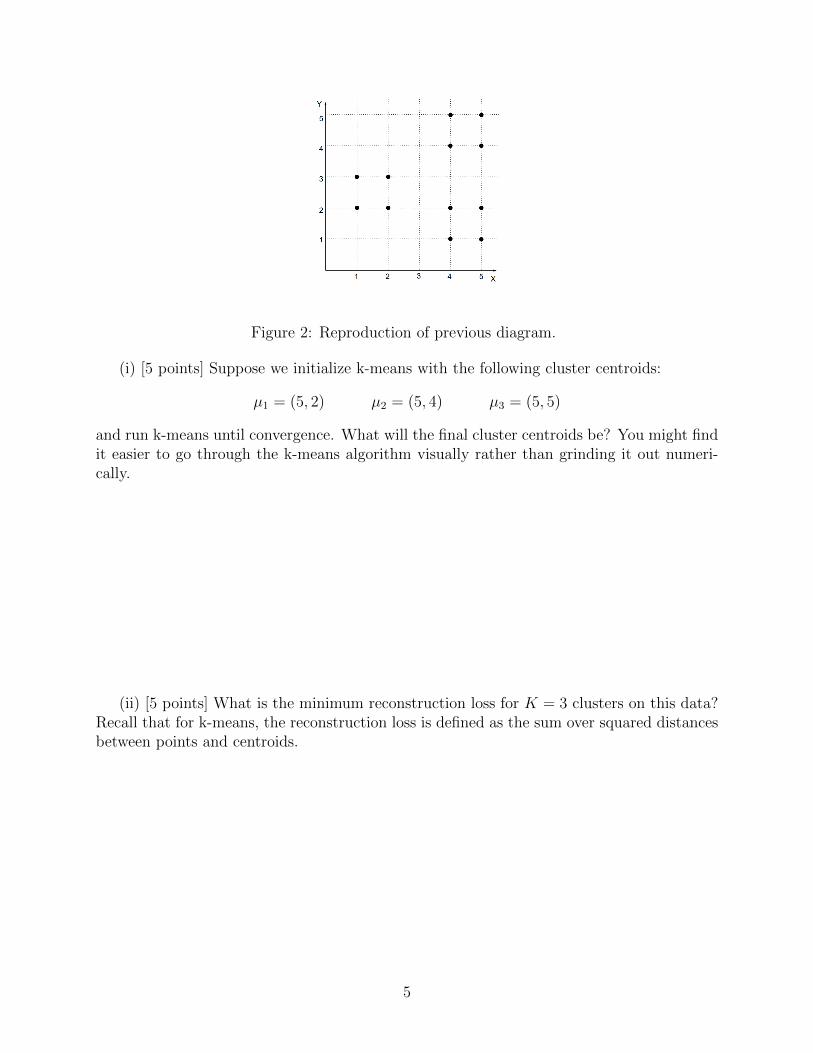
Figure 2: Reproduction of previous diagram.
(i) [5 points] Suppose we initialize k-means with the following cluster centroids:
µ1 = (5, 2) µ2 = (5, 4) µ3 = (5, 5)
and run k-means until convergence. What will the final cluster centroids be? You might find it easier to go through the k-means algorithm visually rather than grinding it out numeri- cally.
(ii) [5 points] What is the minimum reconstruction loss for K = 3 clusters on this data? Recall that for k-means, the reconstruction loss is defined as the sum over squared distances between points and centroids.
5
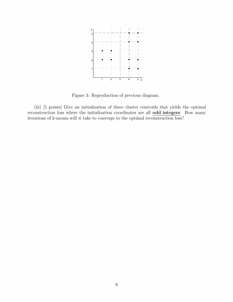
Figure 3: Reproduction of previous diagram.
(iii) [5 points] Give an initialization of three cluster centroids that yields the optimal reconstruction loss where the initialization coordinates are all odd integers. How many iterations of k-means will it take to converge to the optimal reconstruction loss?
6
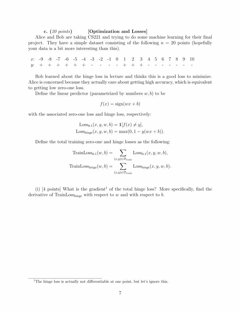
c. (20 points) [Optimization and Losses] Alice and Bob are taking CS221 and trying to do some machine learning for their final
project. They have a simple dataset consisting of the following n = 20 points (hopefully your data is a bit more interesting than this).
x: -9 -8 -7 -6 -5 -4 -3 -2 -1 0 1 2 3 4 5 6 7 8 9 10 y: + + + + + + - - - - + + + - - - - - - -
Bob learned about the hinge loss in lecture and thinks this is a good loss to minimize. Alice is concerned because they actually care about getting high accuracy, which is equivalent to getting low zero-one loss.
Define the linear predictor (parametrized by numbers w, b) to be
f(x) = sign(wx+ b)
Loss0-1(x, y, w, b) = 1[f(x) 6= y],
Losshinge(x, y, w, b) = max(0, 1− y(wx+ b)).
Define the total training zero-one and hinge losses as the following:
TrainLoss0-1(w, b) = ∑
(x,y)∈Dtrain
Losshinge(x, y, w, b).
(i) [4 points] What is the gradient1 of the total hinge loss? More specifically, find the derivative of TrainLosshinge with respect to w and with respect to b.
1The hinge loss is actually not differentiable at one point, but let’s ignore this.
7
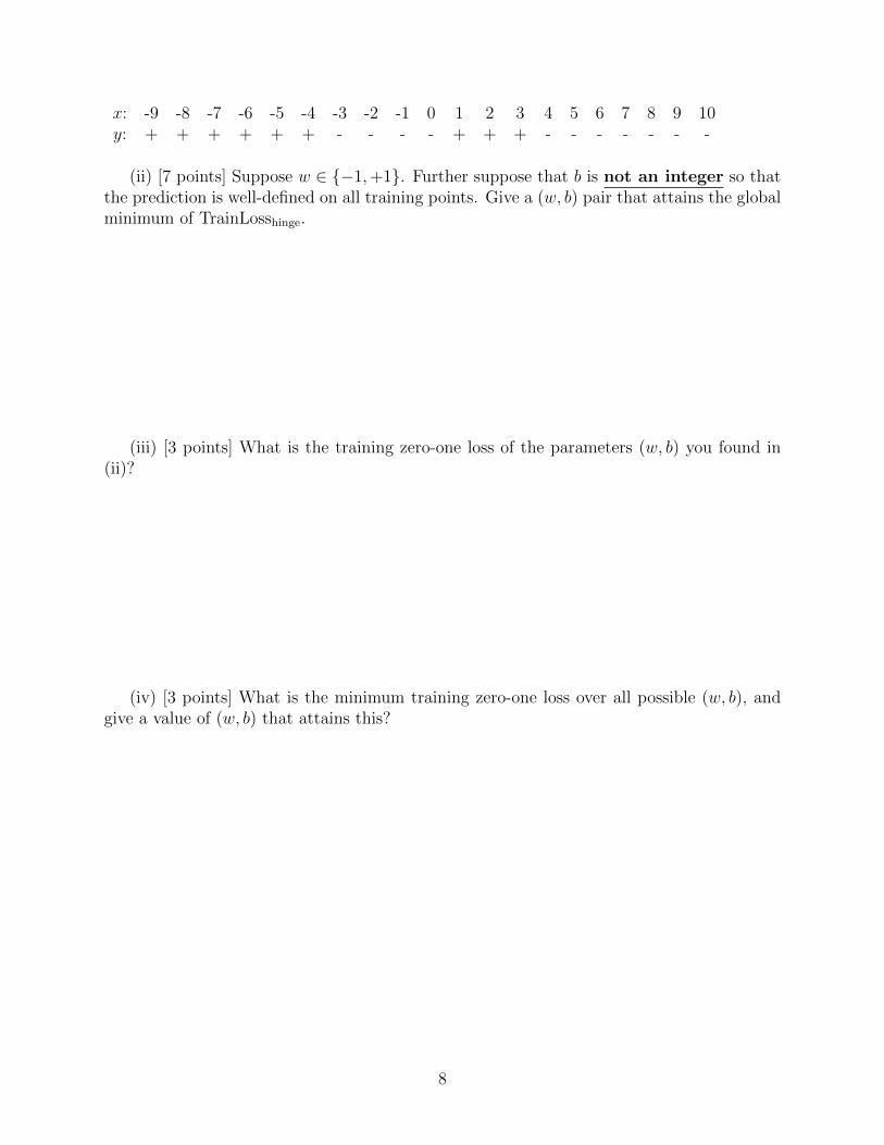
x: -9 -8 -7 -6 -5 -4 -3 -2 -1 0 1 2 3 4 5 6 7 8 9 10 y: + + + + + + - - - - + + + - - - - - - -
(ii) [7 points] Suppose w ∈ {−1,+1}. Further suppose that b is not an integer so that the prediction is well-defined on all training points. Give a (w, b) pair that attains the global minimum of TrainLosshinge.
(iii) [3 points] What is the training zero-one loss of the parameters (w, b) you found in (ii)?
(iv) [3 points] What is the minimum training zero-one loss over all possible (w, b), and give a value of (w, b) that attains this?
8
(v) [3 points] Alice is right in wanting to use the zero-one loss instead of the hinge loss because, in the end, we usually care about accuracy (which is a linear function of the zero- one loss). Give a reason why Bob is right in wanting to use the hinge loss instead of the zero-one loss.
9
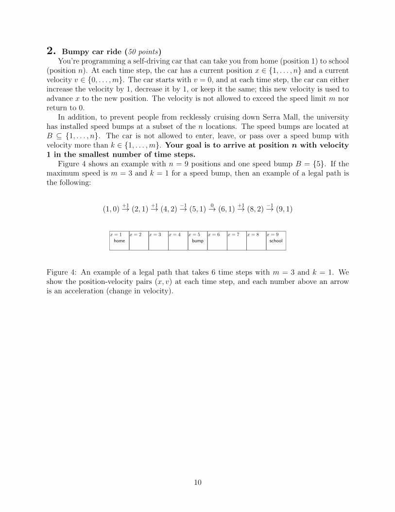
2. Bumpy car ride (50 points) You’re programming a self-driving car that can take you from home (position 1) to school
(position n). At each time step, the car has a current position x ∈ {1, . . . , n} and a current velocity v ∈ {0, . . . ,m}. The car starts with v = 0, and at each time step, the car can either increase the velocity by 1, decrease it by 1, or keep it the same; this new velocity is used to advance x to the new position. The velocity is not allowed to exceed the speed limit m nor return to 0.
In addition, to prevent people from recklessly cruising down Serra Mall, the university has installed speed bumps at a subset of the n locations. The speed bumps are located at B ⊆ {1, . . . , n}. The car is not allowed to enter, leave, or pass over a speed bump with velocity more than k ∈ {1, . . . ,m}. Your goal is to arrive at position n with velocity 1 in the smallest number of time steps.
Figure 4 shows an example with n = 9 positions and one speed bump B = {5}. If the maximum speed is m = 3 and k = 1 for a speed bump, then an example of a legal path is the following:
(1, 0) +1→ (2, 1)
+1→ (4, 2) −1→ (5, 1)
0→ (6, 1) +1→ (8, 2)
−1→ (9, 1)
bump
school
Figure 4: An example of a legal path that takes 6 time steps with m = 3 and k = 1. We show the position-velocity pairs (x, v) at each time step, and each number above an arrow is an acceleration (change in velocity).
10
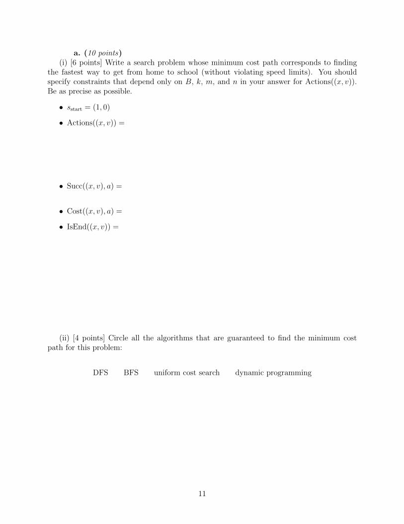
a. (10 points) (i) [6 points] Write a search problem whose minimum cost path corresponds to finding
the fastest way to get from home to school (without violating speed limits). You should specify constraints that depend only on B, k, m, and n in your answer for Actions((x, v)). Be as precise as possible.
• sstart = (1, 0)
• IsEnd((x, v)) =
(ii) [4 points] Circle all the algorithms that are guaranteed to find the minimum cost path for this problem:
DFS BFS uniform cost search dynamic programming
11
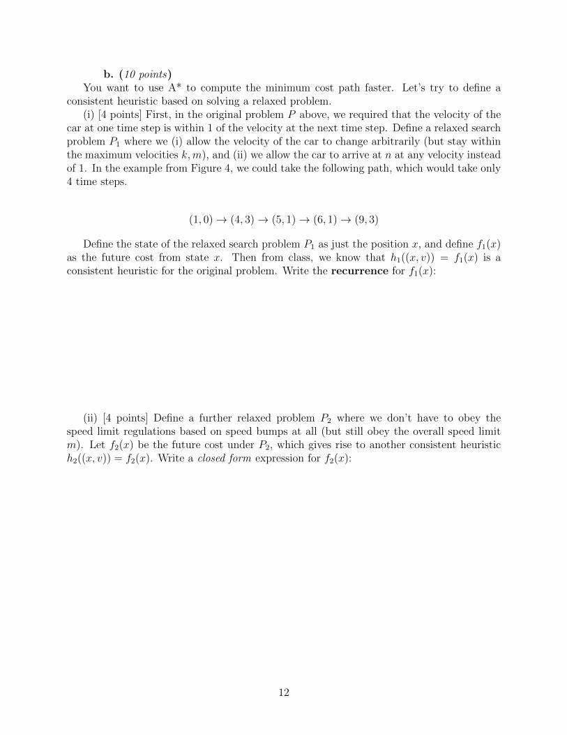
b. (10 points) You want to use A* to compute the minimum cost path faster. Let’s try to define a
consistent heuristic based on solving a relaxed problem. (i) [4 points] First, in the original problem P above, we required that the velocity of the
car at one time step is within 1 of the velocity at the next time step. Define a relaxed search problem P1 where we (i) allow the velocity of the car to change arbitrarily (but stay within the maximum velocities k,m), and (ii) we allow the car to arrive at n at any velocity instead of 1. In the example from Figure 4, we could take the following path, which would take only 4 time steps.
(1, 0)→ (4, 3)→ (5, 1)→ (6, 1)→ (9, 3)
Define the state of the relaxed search problem P1 as just the position x, and define f1(x) as the future cost from state x. Then from class, we know that h1((x, v)) = f1(x) is a consistent heuristic for the original problem. Write the recurrence for f1(x):
(ii) [4 points] Define a further relaxed problem P2 where we don’t have to obey the speed limit regulations based on speed bumps at all (but still obey the overall speed limit m). Let f2(x) be the future cost under P2, which gives rise to another consistent heuristic h2((x, v)) = f2(x). Write a closed form expression for f2(x):
12
(iii) [2 points] Discuss (in two or three sentences) the accuracy/speed tradeoffs of heuris- tics h1 and h2.
13
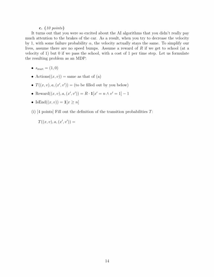
c. (10 points) It turns out that you were so excited about the AI algorithms that you didn’t really pay
much attention to the brakes of the car. As a result, when you try to decrease the velocity by 1, with some failure probability α, the velocity actually stays the same. To simplify our lives, assume there are no speed bumps. Assume a reward of R if we get to school (at a velocity of 1) but 0 if we pass the school, with a cost of 1 per time step. Let us formulate the resulting problem as an MDP:
• sstart = (1, 0)
• Actions((x, v)) = same as that of (a)
• T ((x, v), a, (x′, v′)) = (to be filled out by you below)
• Reward((x, v), a, (x′, v′)) = R · 1[x′ = n ∧ v′ = 1]− 1
• IsEnd((x, v)) = 1[x ≥ n]
(i) [4 points] Fill out the definition of the transition probabilities T :
T ((x, v), a, (x′, v′)) =
14
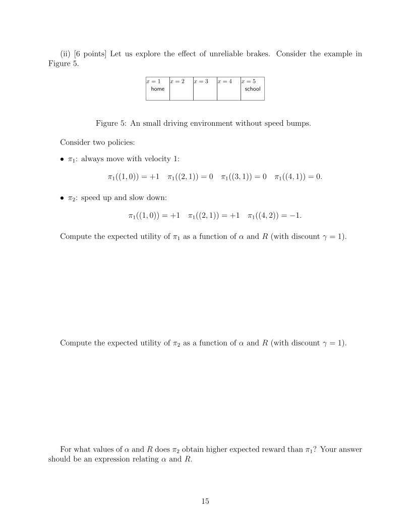
(ii) [6 points] Let us explore the effect of unreliable brakes. Consider the example in Figure 5.
x = 1
school
Consider two policies:
• π1: always move with velocity 1:
π1((1, 0)) = +1 π1((2, 1)) = 0 π1((3, 1)) = 0 π1((4, 1)) = 0.
• π2: speed up and slow down:
π1((1, 0)) = +1 π1((2, 1)) = +1 π1((4, 2)) = −1.
Compute the expected utility of π1 as a function of α and R (with discount γ = 1).
Compute the expected utility of π2 as a function of α and R (with discount γ = 1).
For what values of α and R does π2 obtain higher expected reward than π1? Your answer should be an expression relating α and R.
15
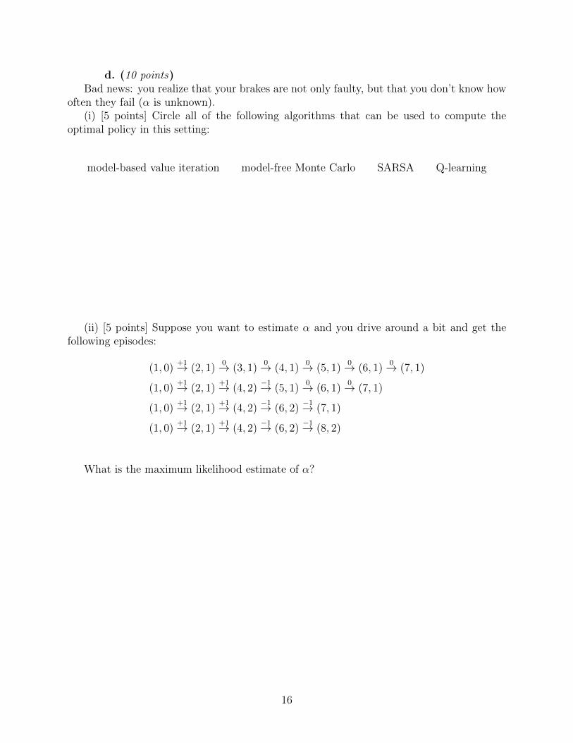
d. (10 points) Bad news: you realize that your brakes are not only faulty, but that you don’t know how
often they fail (α is unknown). (i) [5 points] Circle all of the following algorithms that can be used to compute the
optimal policy in this setting:
model-based value iteration model-free Monte Carlo SARSA Q-learning
(ii) [5 points] Suppose you want to estimate α and you drive around a bit and get the following episodes:
(1, 0) +1→ (2, 1)
0→ (3, 1) 0→ (4, 1)
0→ (5, 1) 0→ (6, 1)
0→ (7, 1)
+1→ (4, 2) −1→ (5, 1)
0→ (6, 1) 0→ (7, 1)
(1, 0) +1→ (2, 1)
+1→ (4, 2) −1→ (6, 2)
−1→ (7, 1)
+1→ (4, 2) −1→ (6, 2)
−1→ (8, 2)
16
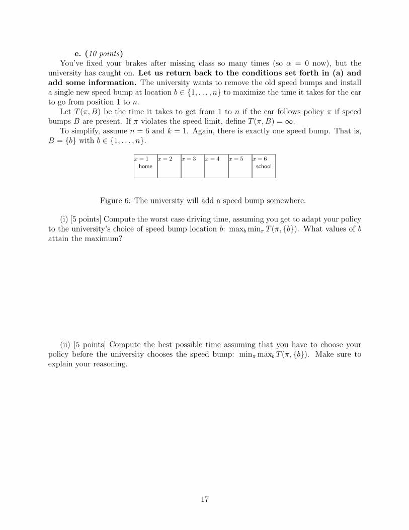
e. (10 points) You’ve fixed your brakes after missing class so many times (so α = 0 now), but the
university has caught on. Let us return back to the conditions set forth in (a) and add some information. The university wants to remove the old speed bumps and install a single new speed bump at location b ∈ {1, . . . , n} to maximize the time it takes for the car to go from position 1 to n.
Let T (π,B) be the time it takes to get from 1 to n if the car follows policy π if speed bumps B are present. If π violates the speed limit, define T (π,B) =∞.
To simplify, assume n = 6 and k = 1. Again, there is exactly one speed bump. That is, B = {b} with b ∈ {1, . . . , n}.
x = 1
x = 2 x = 3 x = 4 x = 5 x = 6
school
Figure 6: The university will add a speed bump somewhere.
(i) [5 points] Compute the worst case driving time, assuming you get to adapt your policy to the university’s choice of speed bump location b: maxb minπ T (π, {b}). What values of b attain the maximum?
(ii) [5 points] Compute the best possible time assuming that you have to choose your policy before the university chooses the speed bump: minπ maxb T (π, {b}). Make sure to explain your reasoning.
17
3. The Bayesian Bag of Candies Model (50 points) You have a lot of candy left over from Halloween, and you decide to give them away
to your friends. You have four types of candy: Apple, Banana, Caramel, Dark-Chocolate. You decide to prepare candy bags using the following process.
• For each candy bag, you first flip a (biased) coin Y which comes up heads (Y = H) with probability λ and tails (Y = T) with probability 1− λ.
• If Y comes up heads (Y = H), you make a Healthy bag, where you:
1. Add one Apple candy with probability p1 or nothing with probability 1− p1; 2. Add one Banana candy with probability p1 or nothing with probability 1− p1; 3. Add one Caramel candy with probability 1− p1 or nothing with probability p1;
4. Add one Dark-Chocolate candy with probability 1−p1 or nothing with probability p1.
• If Y comes up tails (Y = T), you make a Tasty bag, where you:
1. Add one Apple candy with probability p2 or nothing with probability 1− p2; 2. Add one Banana candy with probability p2 or nothing with probability 1− p2; 3. Add one Caramel candy with probability 1− p2 or nothing with probability p2;
4. Add one Dark-Chocolate candy with probability 1−p2 or nothing with probability p2.
For example, if p1 = 1 and p2 = 0, you would deterministically generate: Healthy bags with one Apple and one Banana; and Tasty bags with one Caramel and one Dark-Chocolate. For general values of p1 and p2, bags can contain anywhere between 0 and 4 pieces of candy.
Denote A,B,C,D random variables indicating whether or not the bag contains candy of type Apple, Banana, Caramel, and Dark-Chocolate, respectively.
18
a. (15 points) (i) Draw the Bayesian network corresponding to process of creating a single bag.
(ii) What is the probability of generating a Healthy bag containing Apple, Banana, Caramel, and not Dark-Chocolate? For compactness, we will use the following notation to denote this possible outcome:
(Healthy, {Apple,Banana,Caramel}).
(iii) What is the probability of generating a bag containing Apple, Banana, Caramel, and not Dark-Chocolate?
(iv) What is the probability that a bag was a Tasty one, given that it contains Apple, Banana, Caramel, and not Dark-Chocolate?
19
b. (10 points) You realize you need to make more candy bags, but you’ve forgotten the probabilities
you used to generate them. So you try to estimate them looking at the 5 bags you’ve already made:
bag 1 : (Healthy, {Apple,Banana}) bag 2 : (Tasty, {Caramel,Dark-Chocolate}) bag 3 : (Healthy, {Apple,Banana}) bag 4 : (Tasty, {Caramel,Dark-Chocolate}) bag 5 : (Healthy, {Apple,Banana})
Estimate λ, p1, p2 by maximum likelihood.
Estimate λ, p1, p2 by maximum likelihood, using Laplace smoothing with parameter 1.
20
c. (15 points) You find out your little brother had been playing with your candy bags, and had mixed them up (in a uniformly random way). Now you don’t even know which ones were Healthy and which ones were Tasty. So you need to re-estimate λ, p1, p2, but now without knowing whether the bags were Healthy or Tasty.
bag 1 : (? , {Apple,Banana,Caramel}) bag 2 : (? , {Caramel,Dark-Chocolate}) bag 3 : (? , {Apple,Banana,Caramel}) bag 4 : (? , {Caramel,Dark-Chocolate}) bag 5 : (? , {Apple,Banana,Caramel})
You remember the EM algorithm is just what you need. Initialize with λ = 0.5, p1 = 0.5, p2 = 0, and run one step of the EM algorithm.
(i) E-step:
(ii) M-step:
21
d. (10 points) You decide to make candy bags according to a new process. You create the first one as
described above. Then with probability µ, you create a second bag of the same type as the first one (Healthy or Tasty), and of different type with probability 1 − µ. Given this type, the bag is filled with candy as before. Then with probability µ, you create a third bag of the same type as the second one (Healthy or Tasty), and of different type with probability 1− µ. And so on, you repeat the process M times. Denote Yi, Ai, Bi, Ci, Di the variables at each time step, for i = 0, . . . ,M . Let Xi = (Ai, Bi, Ci, Di).
Now you want to compute:
P(Yi = Healthy | X0 = (1, 1, 1, 0), . . . , Xi = (1, 1, 1, 0))
exactly for all i = 0, . . . ,M , and you decide to use the forward-backward algorithm. Suppose you have already computed the marginals:
fi = P(Yi = Healthy | X0 = (1, 1, 1, 0), . . . , Xi = (1, 1, 1, 0))
for some i ≥ 0. Recall the first step of the algorithm is to compute an intermediate result proportional to
P(Yi+1 | X0 = (1, 1, 1, 0), . . . , Xi = (1, 1, 1, 0), Xi+1 = (1, 1, 1, 0))
(i) Write an expression that is proportional to
P(Yi+1 = Healthy | X0 = (1, 1, 1, 0), . . . , Xi = (1, 1, 1, 0), Xi+1 = (1, 1, 1, 0))
in terms of fi and the parameters p1, p2, λ, µ.
22
(ii) Write an expression that is proportional to
P(Yi+1 = Tasty | X0 = (1, 1, 1, 0), . . . , Xi = (1, 1, 1, 0), Xi+1 = (1, 1, 1, 0))
in terms of fi and the parameters of the model p1, p2, λ, µ. The proportionality constant should be the same as in (i).
(iii) Let h be the answer for part (i), and t for part (ii). Write an expression for
P(Yi+1 = Healthy | X0 = (1, 1, 1, 0), . . . , Xi = (1, 1, 1, 0), Xi+1 = (1, 1, 1, 0))
in terms of h, t and the parameters of the model p1, p2, λ, µ.
Congratulations, you have reached the end of the exam!
23