CS231A Final Project:

Who Drew It? Style Analysis on DeviantART

Mindy Huang (mindyh)Ben-han Sung (bsung93)

Abstract

Our project studied popular portrait artists on Deviant Art and attempted to identify their artwork byidiosyncratic properties such as color palette, texture, and composition. We extracted these properties fromeach artist’s drawings using computer vision methods and used machine learning to discover each artist’sunique style. Notable features include face detection using OpenCV Haar cascades and highlight detectionwith Quickshift segmentation. With logistic regression, we were able to accurately predict whether a workbelonged to an artist with a best F1 score of 0.81.

1 Introduction

As hobbyist artists and computer scientists, we were interested in applying our computer vision skills toanalyze the work of other artists. Our original idea was to study the works of popular portrait artists onDeviant Art - is there something about their use of colors, lines, composition, and other basic techniquesthat makes the rise above the fray? As it turned out, this is a difficult question to answer because popularityof a drawing is often not only by the artist’s skill, but also by the audience. In particular, there are socialfactors at play that are not captured by the artwork itself, such as the number of followers an artist has,what topics are trending, what genres are popular, and so forth.

While trying (and failing) to establish a correlation between a piece of artwork and its popularity, westumbled upon the equally interesting problem of matching art to the artist. This turned into the eventualfocus of our work. Given any drawing, is it possible to predict who drew it?

2 Previous work

This project is similar to the classic machine learning task of identifying the author of the Federalist Papersusing textual analysis. We have applied the same methodology in the art domain, using art features likecomposition and color palette in lieu of linguistic features like word frequency. We focused specifically onportraiture from Deviant Art so as to narrow down the problem domain.

2.1 Review of previous work

The attribution of art to artists is, in fact, a popular topic of machine learning. Most work in this domain areprojects that analyze works done by old masters. Serious projects explore how machine learning can aid arthistorians (ex. Saleh et. al [5]); most others are simpler student projects done primarily for the edificationof the authors (ex. Buter et. al [1]).

1

2.2 Difference from previous work

The novelty of our approach to the art attribution problem comes primarily from our feature selection forthe prediction task. We focused primarily on image content analysis via computer vision techniques suchas preprocessing transformations, image segmentation, and face recognition, and identifying salient features.We then apply various standard binary classifiers to find the best results that we can. We approached thelearning problem with the assumption that a standard classifier could give us good results if we could giveit good set of features.

3 Technical Solution

3.1 Summary

1. Scrape the URLs of artworks from DeviantArt under the Portraits category and save them into a SQLitedatabase.

2. For each URL in our database:

a. download the image

b. scrape the metadata features (ex. Digital or Traditional) and save them to the database

c. extract the feature values from the image

d. save the feature values to the database

3. After we’re done scraping - extract the saved features and train our model on them.

4. Validate our classifier by looking at precision, recall, and F1 score.

3.2 Data Collection and Processing Pipeline

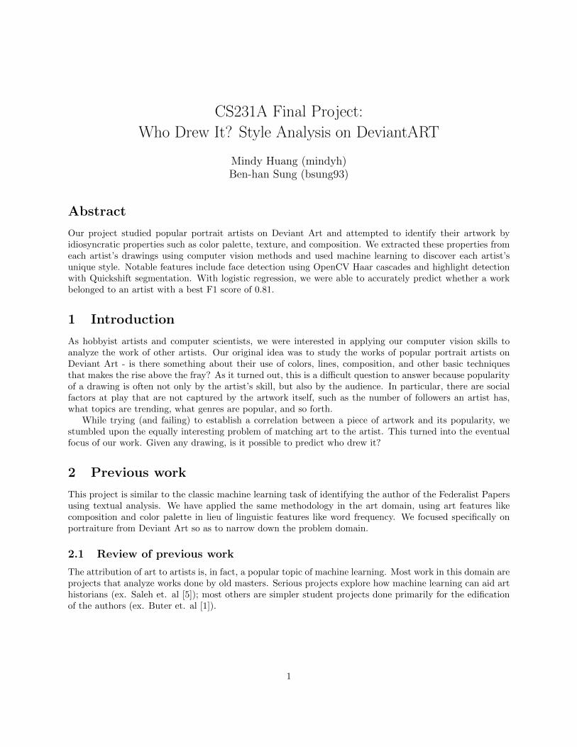
First, we acquired a dataset of 2000 drawings by scraping DeviantArt’s Portraits category as well as thegallery of popular artists. Our scraper saved URLS, views, favorites, and category information to a SQLitedatabase. Then, we ran a feature extraction script which downloaded each image and ran the featureextractors over them. The resulting values were stored in the in the corresponding column in the database.Altogether we had approximately 100 column-features (because some high-level features like color werebinned and broken across several columns).

Figure 1: Example of our database

Afterwards, it was just a matter of piping the information from the database into scikit-learn for ourmachine learning layer.

2

3.3 Features

The brunt of our project revolves around using computer vision techniques to extract features from eachportrait. We wanted to make sure that our features captured the ’style’ of each image. After some brain-storming, we ended up defined ’style’ as choices around Composition, Color Palette, Texture, and Lighting.This is obviously not an exhaustive list, but just what we determined was an appropriate scope for thisproject.

3.3.1 Face/Eye Detection

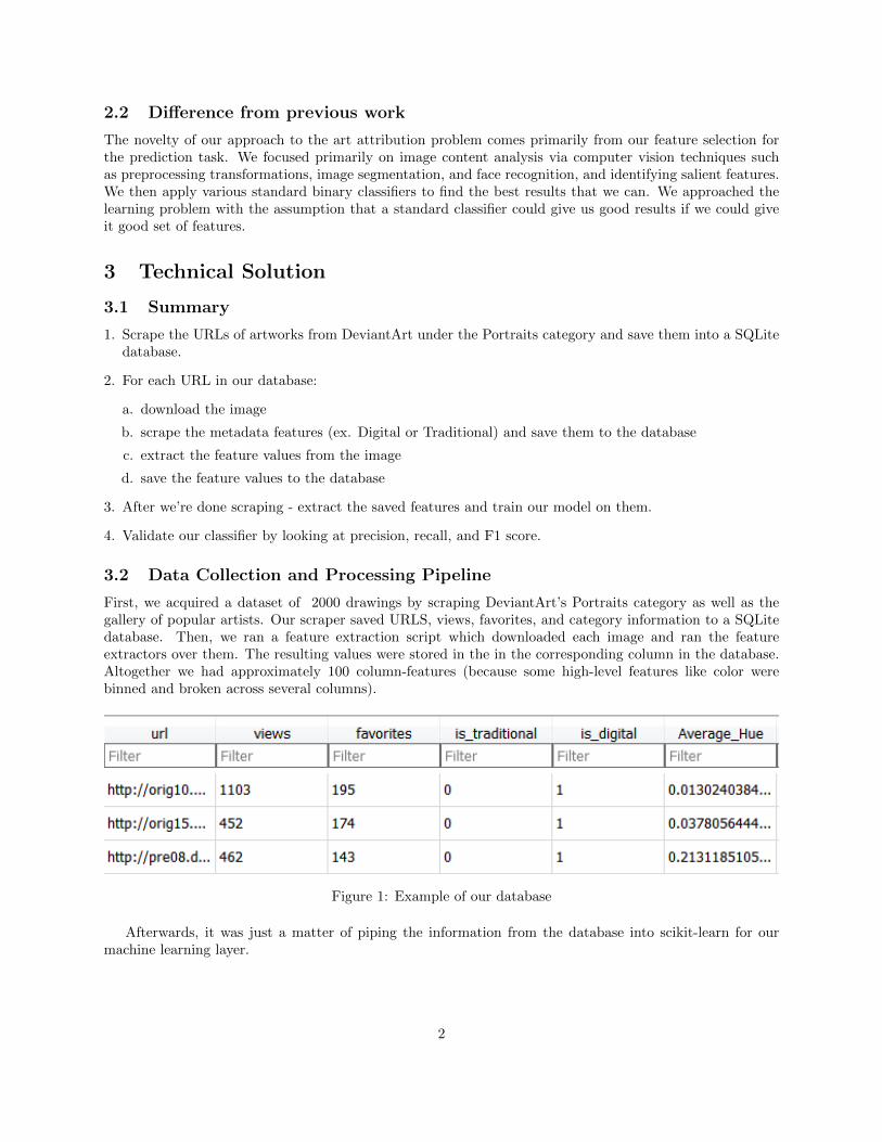
We tried to capture composition through objectdetection. We had many detectors (hands, ears,nose, smile, profile face) based primarily on OpenCVHaar cascades, but our frontal face and eye detectionworked best. Figure 2.

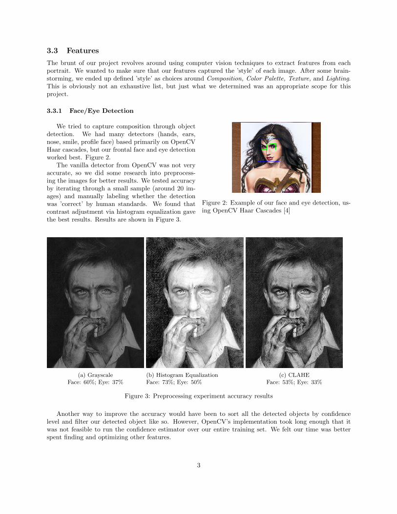
The vanilla detector from OpenCV was not veryaccurate, so we did some research into preprocess-ing the images for better results. We tested accuracyby iterating through a small sample (around 20 im-ages) and manually labeling whether the detectionwas ’correct’ by human standards. We found thatcontrast adjustment via histogram equalization gavethe best results. Results are shown in Figure 3.

Figure 2: Example of our face and eye detection, us-ing OpenCV Haar Cascades [4]

(a) GrayscaleFace: 60%; Eye: 37%

(b) Histogram EqualizationFace: 73%; Eye: 50%

(c) CLAHEFace: 53%; Eye: 33%

Figure 3: Preprocessing experiment accuracy results

Another way to improve the accuracy would have been to sort all the detected objects by confidencelevel and filter our detected object like so. However, OpenCV’s implementation took long enough that itwas not feasible to run the confidence estimator over our entire training set. We felt our time was betterspent finding and optimizing other features.

3

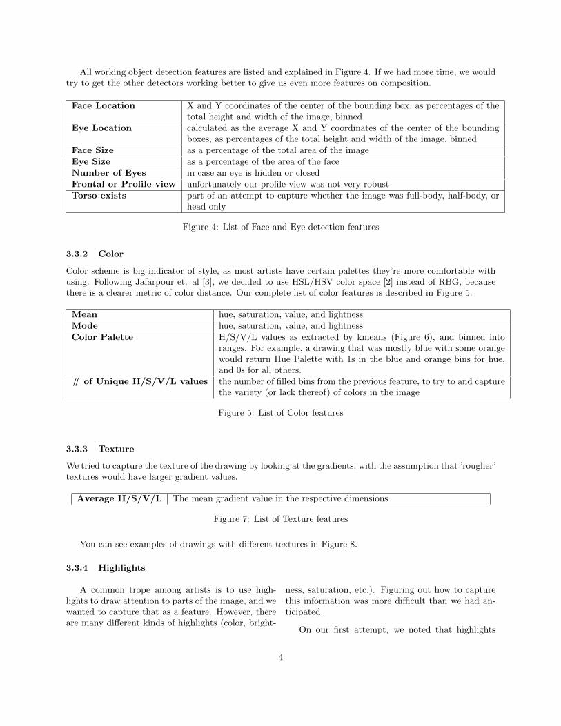
All working object detection features are listed and explained in Figure 4. If we had more time, we wouldtry to get the other detectors working better to give us even more features on composition.

Face Location X and Y coordinates of the center of the bounding box, as percentages of thetotal height and width of the image, binned

Eye Location calculated as the average X and Y coordinates of the center of the boundingboxes, as percentages of the total height and width of the image, binned

Face Size as a percentage of the total area of the imageEye Size as a percentage of the area of the faceNumber of Eyes in case an eye is hidden or closedFrontal or Profile view unfortunately our profile view was not very robustTorso exists part of an attempt to capture whether the image was full-body, half-body, or

head only

Figure 4: List of Face and Eye detection features

3.3.2 Color

Color scheme is big indicator of style, as most artists have certain palettes they’re more comfortable withusing. Following Jafarpour et. al [3], we decided to use HSL/HSV color space [2] instead of RBG, becausethere is a clearer metric of color distance. Our complete list of color features is described in Figure 5.

Mean hue, saturation, value, and lightnessMode hue, saturation, value, and lightnessColor Palette H/S/V/L values as extracted by kmeans (Figure 6), and binned into

ranges. For example, a drawing that was mostly blue with some orangewould return Hue Palette with 1s in the blue and orange bins for hue,and 0s for all others.

# of Unique H/S/V/L values the number of filled bins from the previous feature, to try to and capturethe variety (or lack thereof) of colors in the image

Figure 5: List of Color features

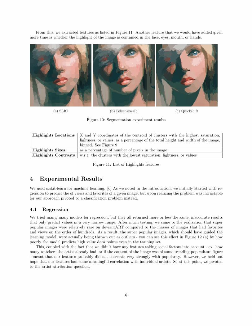
3.3.3 Texture

We tried to capture the texture of the drawing by looking at the gradients, with the assumption that ’rougher’textures would have larger gradient values.

Average H/S/V/L The mean gradient value in the respective dimensions

Figure 7: List of Texture features

You can see examples of drawings with different textures in Figure 8.

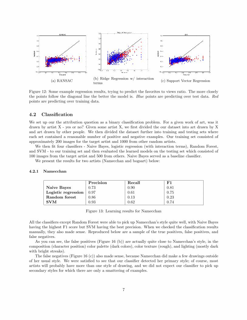
3.3.4 Highlights

A common trope among artists is to use high-lights to draw attention to parts of the image, and wewanted to capture that as a feature. However, thereare many different kinds of highlights (color, bright-

ness, saturation, etc.). Figuring out how to capturethis information was more difficult than we had an-ticipated.

On our first attempt, we noted that highlights

4

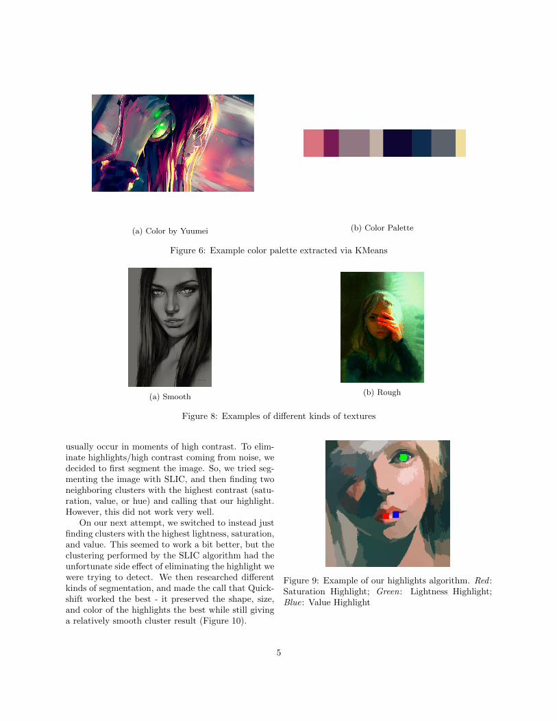
(a) Color by Yuumei (b) Color Palette

Figure 6: Example color palette extracted via KMeans

(a) Smooth(b) Rough

Figure 8: Examples of different kinds of textures

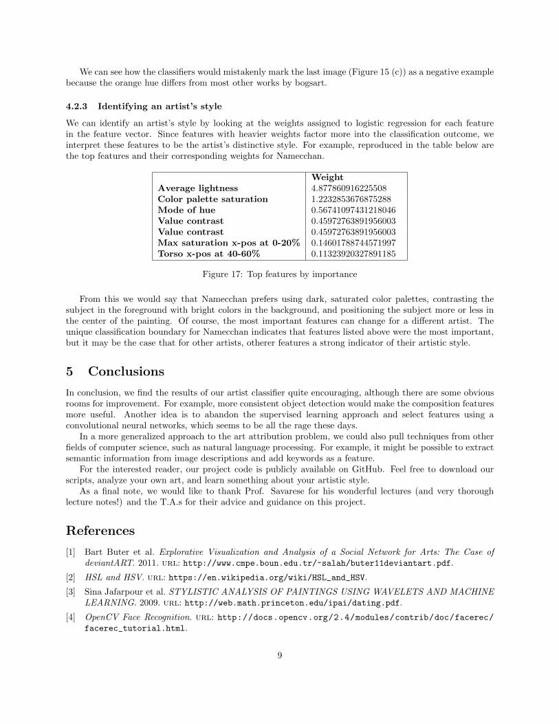
usually occur in moments of high contrast. To elim-inate highlights/high contrast coming from noise, wedecided to first segment the image. So, we tried seg-menting the image with SLIC, and then finding twoneighboring clusters with the highest contrast (satu-ration, value, or hue) and calling that our highlight.However, this did not work very well.

On our next attempt, we switched to instead justfinding clusters with the highest lightness, saturation,and value. This seemed to work a bit better, but theclustering performed by the SLIC algorithm had theunfortunate side effect of eliminating the highlight wewere trying to detect. We then researched differentkinds of segmentation, and made the call that Quick-shift worked the best - it preserved the shape, size,and color of the highlights the best while still givinga relatively smooth cluster result (Figure 10).

Figure 9: Example of our highlights algorithm. Red :Saturation Highlight; Green: Lightness Highlight;Blue: Value Highlight

5

From this, we extracted features as listed in Figure 11. Another feature that we would have added givenmore time is whether the highlight of the image is contained in the face, eyes, mouth, or hands.

(a) SLIC (b) Felzenszwalb (c) Quickshift

Figure 10: Segmentation experiment results

Highlights Locations X and Y coordinates of the centroid of clusters with the highest saturation,lightness, or values, as a percentage of the total height and width of the image,binned. See Figure 9

Highlights Sizes as a percentage of number of pixels in the imageHighlights Contrasts w.r.t. the clusters with the lowest saturation, lightness, or values

Figure 11: List of Highlights features

4 Experimental Results

We used scikit-learn for machine learning. [6] As we noted in the introduction, we initially started with re-gression to predict the of views and favorites of a given image, but upon realizing the problem was intractablefor our approach pivoted to a classification problem instead.

4.1 Regression

We tried many, many models for regression, but they all returned more or less the same, inaccurate resultsthat only predict values in a very narrow range. After much testing, we came to the realization that superpopular images were relatively rare on deviantART compared to the masses of images that had favoritesand views on the order of hundreds. As a result, the super popular images, which should have guided thelearning model, were actually being thrown out as outliers - you can see this effect in Figure 12 (a) by howpoorly the model predicts high value data points even in the training set.

This, coupled with the fact that we didn’t have any features taking social factors into account - ex. howmany watchers the artist already had, or if the content of the image was of some trending pop culture figure- meant that our features probably did not correlate very strongly with popularity. However, we held outhope that our features had some meaningful correlation with individual artists. So at this point, we pivotedto the artist attribution question.

6

(a) RANSAC(b) Ridge Regression w/ interactionterms

(c) Support Vector Regression

Figure 12: Some example regression results, trying to predict the favorites to views ratio. The more closelythe points follow the diagonal line the better the model is. Blue points are predicting over test data. Redpoints are predicting over training data.

4.2 Classification

We set up our the attribution question as a binary classification problem. For a given work of art, was itdrawn by artist X - yes or no? Given some artist X, we first divided the our dataset into art drawn by Xand art drawn by other people. We then divided the dataset further into training and testing sets whereeach set contained a reasonable number of positive and negative examples. Our training set consisted ofapproximately 200 images for the target artist and 1000 from other random artists.

We then fit four classifiers - Naive Bayes, logistic regression (with interaction terms), Random Forest,and SVM - to our training set and then evaluated the learned models on the testing set which consisted of100 images from the target artist and 500 from others. Naive Bayes served as a baseline classifier.

We present the results for two artists (Namecchan and bogsart) below:

4.2.1 Namecchan

Precision Recall F1Naive Bayes 0.73 0.90 0.81Logistic regression 0.97 0.61 0.75Random forest 0.86 0.13 0.23SVM 0.93 0.62 0.74

Figure 13: Learning results for Namecchan

All the classifiers except Random Forest were able to pick up Namecchan’s style quite well, with Naive Bayeshaving the highest F1 score but SVM having the best precision. When we checked the classification resultsmanually, they also made sense. Reproduced below are a sample of the true positives, false positives, andfalse negatives.

As you can see, the false positives (Figure 16 (b)) are actually quite close to Namecchan’s style, in thecomposition (character position) color palette (dark colors), color texture (rough), and lighting (mostly darkwith bright streaks).

The false negatives (Figure 16 (c)) also made sense, because Namecchan did make a few drawings outsideof her usual style. We were satisfied to see that our classifier detected her primary style; of course, mostartists will probably have more than one style of drawing, and we did not expect our classifier to pick upsecondary styles for which there are only a smattering of examples.

7

(a) True positive(b) False positive

(c) False negative

Figure 14: Prediction results for Namecchan

4.2.2 bogsart

Precision Recall F1Naive Bayes 0.17 0.94 0.29Logistic regression 0.42 0.73 0.53Random forest 0.62 0.71 0.66SVM 0.49 0.75 0.59

Figure 15: Learning results for bogsart

It turns out that bogsart’s style was harder to identify. We think that this was because he drew mainlyblack and white charcoal sketches. This means that our color and highlight features would have troubledistinguishing his work from other black and white artists; furthermore, the texture in his drawing comesmainly from the medium (charcoal), so that is not very distinctive either. As you can see, our classifiersidentified some very similar charcoal drawings (Figure 15 (b)) as false positives.

(a) True positive(b) False positive (c) False negative

Figure 16: Prediction results for bogsart

8

We can see how the classifiers would mistakenly mark the last image (Figure 15 (c)) as a negative examplebecause the orange hue differs from most other works by bogsart.

4.2.3 Identifying an artist’s style

We can identify an artist’s style by looking at the weights assigned to logistic regression for each featurein the feature vector. Since features with heavier weights factor more into the classification outcome, weinterpret these features to be the artist’s distinctive style. For example, reproduced in the table below arethe top features and their corresponding weights for Namecchan.

WeightAverage lightness 4.877860916225508Color palette saturation 1.2232853676875288Mode of hue 0.56741097431218046Value contrast 0.45972763891956003Value contrast 0.45972763891956003Max saturation x-pos at 0-20% 0.14601788744571997Torso x-pos at 40-60% 0.11323920327891185

Figure 17: Top features by importance

From this we would say that Namecchan prefers using dark, saturated color palettes, contrasting thesubject in the foreground with bright colors in the background, and positioning the subject more or less inthe center of the painting. Of course, the most important features can change for a different artist. Theunique classification boundary for Namecchan indicates that features listed above were the most important,but it may be the case that for other artists, otherer features a strong indicator of their artistic style.

5 Conclusions

In conclusion, we find the results of our artist classifier quite encouraging, although there are some obviousrooms for improvement. For example, more consistent object detection would make the composition featuresmore useful. Another idea is to abandon the supervised learning approach and select features using aconvolutional neural networks, which seems to be all the rage these days.

In a more generalized approach to the art attribution problem, we could also pull techniques from otherfields of computer science, such as natural language processing. For example, it might be possible to extractsemantic information from image descriptions and add keywords as a feature.

For the interested reader, our project code is publicly available on GitHub. Feel free to download ourscripts, analyze your own art, and learn something about your artistic style.

As a final note, we would like to thank Prof. Savarese for his wonderful lectures (and very thoroughlecture notes!) and the T.A.s for their advice and guidance on this project.

References

[1] Bart Buter et al. Explorative Visualization and Analysis of a Social Network for Arts: The Case ofdeviantART. 2011. url: http://www.cmpe.boun.edu.tr/~salah/buter11deviantart.pdf.

[2] HSL and HSV. url: https://en.wikipedia.org/wiki/HSL_and_HSV.

[3] Sina Jafarpour et al. STYLISTIC ANALYSIS OF PAINTINGS USING WAVELETS AND MACHINELEARNING. 2009. url: http://web.math.princeton.edu/ipai/dating.pdf.

[4] OpenCV Face Recognition. url: http://docs.opencv.org/2.4/modules/contrib/doc/facerec/facerec_tutorial.html.

9

[5] Babak Saleh et al. “Toward Automated Discovery of Artistic Influence”. In: CoRR abs/1408.3218 (2014).url: http://arxiv.org/abs/1408.3218.

[6] Scikit-learn. url: http://scikit-learn.org/.

10