csaxs notes v1.02 (march 18th, 2011) - paul scherrer institute · csaxs notes v1.02 (march 18th,...

cSAXS notes v1.02 (March 18th, 2011)When all else fails, read the instructions.

For further questions please contact Ana Diaz, Andreas Menzel, or Oliver Bunk.

This document as PDF file:http://www.psi.ch/sls/csaxs/ManualsEN/csaxs_notes.pdf

Contents

Contents 1

1 Common sense 4

2 Preparation of your beamtime 42.1 Date of arrival and departure . . . . . . . . . . . . . . . . . . . . . . . . 42.2 Dosimeter and badge . . . . . . . . . . . . . . . . . . . . . . . . . . . . 42.3 Guest house reservation . . . . . . . . . . . . . . . . . . . . . . . . . . . 52.4 Computer based safety training . . . . . . . . . . . . . . . . . . . . . . . 52.5 Tea, espresso and guest network at the beamline . . . . . . . . . . . . . . 52.6 Power sockets in Switzerland . . . . . . . . . . . . . . . . . . . . . . . . 52.7 Guest bicycles . . . . . . . . . . . . . . . . . . . . . . . . . . . . . . . . 52.8 Beamline web pages . . . . . . . . . . . . . . . . . . . . . . . . . . . . 5

3 Control system 63.1 Console (PC) login: e-account . . . . . . . . . . . . . . . . . . . . . . . 63.2 Data analysis PCs . . . . . . . . . . . . . . . . . . . . . . . . . . . . . . 63.3 Data storage . . . . . . . . . . . . . . . . . . . . . . . . . . . . . . . . . 63.4 Startup of spec . . . . . . . . . . . . . . . . . . . . . . . . . . . . . . . 73.5 spec documentation and help . . . . . . . . . . . . . . . . . . . . . . . 73.6 spec log and data file . . . . . . . . . . . . . . . . . . . . . . . . . . . 73.7 Data directories . . . . . . . . . . . . . . . . . . . . . . . . . . . . . . . 73.8 Basic spec commands . . . . . . . . . . . . . . . . . . . . . . . . . . . 83.9 Burst scans . . . . . . . . . . . . . . . . . . . . . . . . . . . . . . . . . 103.10 Continuous scans . . . . . . . . . . . . . . . . . . . . . . . . . . . . . . 113.11 SMS notification . . . . . . . . . . . . . . . . . . . . . . . . . . . . . . 12

4 Beamline components and how to control them 124.1 Insertion device (U19 undulator) . . . . . . . . . . . . . . . . . . . . . . 12

4.1.1 Technical data . . . . . . . . . . . . . . . . . . . . . . . . . . . 134.1.2 Control . . . . . . . . . . . . . . . . . . . . . . . . . . . . . . . 13

4.2 Front end beam shutter . . . . . . . . . . . . . . . . . . . . . . . . . . . 134.3 CVD diamond filter . . . . . . . . . . . . . . . . . . . . . . . . . . . . . 144.4 Slit systems . . . . . . . . . . . . . . . . . . . . . . . . . . . . . . . . . 14


4.5 Front end filters . . . . . . . . . . . . . . . . . . . . . . . . . . . . . . . 15

1

http://www.psi.ch/sls/csaxs/ManualsEN/csaxs_notes.pdf

4.6 Monochromator . . . . . . . . . . . . . . . . . . . . . . . . . . . . . . . 154.6.1 Technical data . . . . . . . . . . . . . . . . . . . . . . . . . . . 154.6.2 Control . . . . . . . . . . . . . . . . . . . . . . . . . . . . . . . 154.6.3 Energy scans . . . . . . . . . . . . . . . . . . . . . . . . . . . . 16

4.7 Mirror . . . . . . . . . . . . . . . . . . . . . . . . . . . . . . . . . . . . 164.7.1 Technical data . . . . . . . . . . . . . . . . . . . . . . . . . . . 164.7.2 Control . . . . . . . . . . . . . . . . . . . . . . . . . . . . . . . 16

4.8 End station beam shutter . . . . . . . . . . . . . . . . . . . . . . . . . . 174.9 Optical tables . . . . . . . . . . . . . . . . . . . . . . . . . . . . . . . . 17


4.10 Exposure box filters . . . . . . . . . . . . . . . . . . . . . . . . . . . . . 184.11 Exposure box fast shutter . . . . . . . . . . . . . . . . . . . . . . . . . . 194.12 Hexapod . . . . . . . . . . . . . . . . . . . . . . . . . . . . . . . . . . . 19


4.13 Air bearing rotation stage . . . . . . . . . . . . . . . . . . . . . . . . . . 204.14 Piezo . . . . . . . . . . . . . . . . . . . . . . . . . . . . . . . . . . . . 21

4.14.1 Macros . . . . . . . . . . . . . . . . . . . . . . . . . . . . . . . 214.15 Detector flight tube lengths . . . . . . . . . . . . . . . . . . . . . . . . . 224.16 Light curtain . . . . . . . . . . . . . . . . . . . . . . . . . . . . . . . . . 224.17 PILATUS detector . . . . . . . . . . . . . . . . . . . . . . . . . . . . . 23

4.17.1 Technical data . . . . . . . . . . . . . . . . . . . . . . . . . . . 234.17.2 Control . . . . . . . . . . . . . . . . . . . . . . . . . . . . . . . 234.17.3 Macro overview . . . . . . . . . . . . . . . . . . . . . . . . . . 244.17.4 Region of interest . . . . . . . . . . . . . . . . . . . . . . . . . . 244.17.5 Startup and shutdown procedure . . . . . . . . . . . . . . . . . . 244.17.6 Threshold . . . . . . . . . . . . . . . . . . . . . . . . . . . . . . 25

4.18 Cyberstar scintillation point detector . . . . . . . . . . . . . . . . . . . . 264.19 Flat single APD . . . . . . . . . . . . . . . . . . . . . . . . . . . . . . . 264.20 Amptek XR-100CR detector and PX4 pulse processing unit . . . . . . . . 27

4.20.1 Maro overview . . . . . . . . . . . . . . . . . . . . . . . . . . . 274.20.2 Startup procedure . . . . . . . . . . . . . . . . . . . . . . . . . . 28

4.21 Multi channel scaler (MCS) . . . . . . . . . . . . . . . . . . . . . . . . . 284.21.1 Macro overview . . . . . . . . . . . . . . . . . . . . . . . . . . 28

4.22 X-ray eye and similar cameras . . . . . . . . . . . . . . . . . . . . . . . 294.23 Fingerlakes Instrumentation ProLine CCD . . . . . . . . . . . . . . . . . 294.24 Analog and digital I/O . . . . . . . . . . . . . . . . . . . . . . . . . . . 30

4.24.1 DAC pseudo motor . . . . . . . . . . . . . . . . . . . . . . . . . 314.25 Digital delay generators . . . . . . . . . . . . . . . . . . . . . . . . . . . 314.26 Temperature controller . . . . . . . . . . . . . . . . . . . . . . . . . . . 314.27 Teslameter . . . . . . . . . . . . . . . . . . . . . . . . . . . . . . . . . . 314.28 Syringe pumps . . . . . . . . . . . . . . . . . . . . . . . . . . . . . . . 31

4.28.1 Cetoni neMESYS syringe pumps . . . . . . . . . . . . . . . . . 314.28.1.1 Technical data . . . . . . . . . . . . . . . . . . . . . . 314.28.1.2 Macro overview . . . . . . . . . . . . . . . . . . . . . 32

2

4.28.2 Hamilton syringe pumps PSD/4 . . . . . . . . . . . . . . . . . . 334.29 EPICS interface . . . . . . . . . . . . . . . . . . . . . . . . . . . . . . . 344.30 Julabo closed cycle water chillers . . . . . . . . . . . . . . . . . . . . . . 354.31 Oxford cryojet . . . . . . . . . . . . . . . . . . . . . . . . . . . . . . . . 354.32 Lambda Genesys power supplies . . . . . . . . . . . . . . . . . . . . . . 35

5 Matlab (plotting and analysis) 355.1 Online viewer . . . . . . . . . . . . . . . . . . . . . . . . . . . . . . . . 365.2 Example: how to get azimuthally integrated data . . . . . . . . . . . . . 36

5.2.1 Valid pixel mask . . . . . . . . . . . . . . . . . . . . . . . . . . 365.2.2 Including the beamstop in the valid pixel mask . . . . . . . . . . 375.2.3 Determining the beam center . . . . . . . . . . . . . . . . . . . . 375.2.4 Preparing the integration masks . . . . . . . . . . . . . . . . . . 375.2.5 Integrating a range of scans . . . . . . . . . . . . . . . . . . . . 385.2.6 Plotting radially integrated data . . . . . . . . . . . . . . . . . . 385.2.7 Removing hot pixels from the valid pixel mask . . . . . . . . . . 385.2.8 Determining the sample to detector distance using silver behenate 39

6 Chemistry lab. 39

7 Troubleshooting / Frequently Asked Questions 40

A History 42

B Phone list 43

C Guest network 43

D Data transfer 43D.1 File systems . . . . . . . . . . . . . . . . . . . . . . . . . . . . . . . . . 43D.2 Data transfer . . . . . . . . . . . . . . . . . . . . . . . . . . . . . . . . . 44

D.2.1 Mounting drives . . . . . . . . . . . . . . . . . . . . . . . . . . 44D.2.2 Formating drives under Linux . . . . . . . . . . . . . . . . . . . 44D.2.3 Access rights for pre-formated Linux drives . . . . . . . . . . . . 44D.2.4 Compressing data . . . . . . . . . . . . . . . . . . . . . . . . . . 44D.2.5 Transferring data using rsync . . . . . . . . . . . . . . . . . . . . 45D.2.6 Related informations . . . . . . . . . . . . . . . . . . . . . . . . 45

D.3 Windows specific information . . . . . . . . . . . . . . . . . . . . . . . 45D.3.1 Formating drives . . . . . . . . . . . . . . . . . . . . . . . . . . 45D.3.2 Mounting the e-account on the file server . . . . . . . . . . . . . 45

E Where to eat 45

F Public transport 46

Index 46

3

1 Common sense

Common sense and a certain sense of responsibility are essential for working at thecSAXS beamline. Examples are:

• There is no cleaning service apart from the floor being cleaned once a week. Thelocal contacts try to bring the beamline in a resonable state for you and we expectthat you leave the beamline in a at least as reasonable state. In other words: Localcontacts are researchers like you and not your private cleaning staff.

• cSAXS has no standardized experimental setup. Working at the beamline meansresearch and in research you can not expect foolproof designs or a point-and-clickway from the measurements to the final analysis. Please think before acting.

• Please think before acting . . . !

• Each user is happy to find a well equipped toolbox and a well equipped chemistrylab. Please maintain this state by putting back all equipment to its original placebefore leaving.

• Please report all damage (whether it is caused by you or others).

• Please do not use or store chemicals in the control or user preparation room. Pleasedo not mess around with chemicals in the experimental hutch. Please take care thatall chemicals and samples are disposed in a proper way.

• Please remove all your belongings - not less and not more. One item more or lessper user group makes a complete mess over one year . . .

There are many more examples and common sense means that we do not have to listthem all. Thank you for reading and following this section!

2 Preparation of your beamtime

Apart from discussing the experiment with your local contact well in advance some ad-ministrative tasks have to be completed before arrival at PSI.

2.1 Date of arrival and departure

For an efficient use of your beamtime you must arrive on the day before your beamtimestarts and plan for some time in the end for removing your experiment, transferring dataetc.

2.2 Dosimeter and badge

ALL users MUST apply for dosimeter and badge via the digital user office (DUO) PRIORto their arrival at PSI: http://duo.psi.ch.

4

http://duo.psi.ch

2.3 Guest house reservation

Please reserve your guest-house on-line:http://services.web.psi.ch/services/lodging/lodging.html

2.4 Computer based safety training

A computer based safety training has to be attended on site. The course is available inPowerPoint format on-line as well underhttp://srp.web.psi.ch/su-introduction/Einfuehrung_Experimentatoren_englisch.pps. At theend of this course, printing the form confirming that you attended it can only done fromthe single training PC set up for this. If you use the online version then please print theform directly from the pdf-filehttp://sls.web.psi.ch/view.php/beamlines/cs/manuals/proof_of_carrying_out_the_test.pdf.

2.5 Tea, espresso and guest network at the beamline

You will find facilities for preparing tea and espresso from capsules (currently 1CHF/capsule) at the beamline as well as mugs and glasses. The opening hours of thecafeteria and canteen can be found in the appendix, section E. A fridge for food and softdrinks is available at the beamline. Please use common sense in combining food, drinkand work. Otherwise we will be forced to forbid this combination in general for all usersin all rooms of the beamline.

An open wireless LAN is available, see appendix, section C.

2.6 Power sockets in Switzerland

Voltage and frequency are 230 V, 50 Hz.Switzerland has power sockets which differ from most other countries in the world

including the US, Japan, France and Germany. Please search for ‘SEV 1011’ inhttp://en.wikipedia.org/wiki/Power_socket or have a look at the Ger-man pages http://de.wikipedia.org/wiki/Stecker-Typ_J. Two pin ‘eu-roplugs’ will fit. We have a few adapters to the German/French ‘Schuko’ (Schutzkontakt)system CEE 7/4.

We can provide cables with Swiss plugs and IEC C13 connectors, seehttp://en.wikipedia.org/wiki/IEC_connector.

2.7 Guest bicycles

There is a limited number of bikes for users of the PSI large scale facilities available freeof charge. Please ask at the user office near by the reception west.

2.8 Beamline web pages

The cSAXS home page can be found athttp://www.psi.ch/sls/csaxs/csaxs .

5

http://services.web.psi.ch/services/lodging/lodging.html

http://srp.web.psi.ch/su-introduction/Einfuehrung_Experimentatoren_englisch.pps

http://sls.web.psi.ch/view.php/beamlines/cs/manuals/proof_of_carrying_out_the_test.pdf

http://en.wikipedia.org/wiki/Power_socket

http://de.wikipedia.org/wiki/Stecker-Typ_J

http://en.wikipedia.org/wiki/IEC_connector

http://www.psi.ch/sls/csaxs/csaxs

It includes among others a staff list with pictureshttp://www.psi.ch/sls/csaxs/people ,a brief description of standard experimental setup,http://www.psi.ch/sls/csaxs/endstations ,a section called manuals that includes the current documenthttp://www.psi.ch/sls/csaxs/manuals ,our base package of Matlab macros, see also section 5,http://www.psi.ch/sls/csaxs/software ,and a list of publicationshttp://www.psi.ch/sls/csaxs/manuals.

3 Control system

The user front end of the control system is the command line driven program spechttp://www.certif.com. Some hardware in the experimental hutch is controlleddirectly by spec. All other hardware is controlled by EPICS via the spec interface.

3.1 Console (PC) login: e-account

In the e-mail with the first invitation for your beamtime the main proposer received username and password for a so called e-account. Log on with this account to all Linux PCsif your local contact has not already done this for you.

3.2 Data analysis PCs

There are four PCs in the control room, three running Linux and one running Windows.It is suggested to use x12sa-cons-1 for experiment control and x12sa-comp-1 andx12sa-comp-2 for data analysis. The data analysis should be performed by logging onfrom these PCs to x12sa-cn-1, -2, or -3. Each compute node has twelve CPU cores,96 GB of RAM and fast access to the file server, i.e., you can for example run severalMatlab sessions in parallel or use parallel and distributed computing. The Windows PC isavailable to run specialized software like a frame grabber.

The file server is always accessible via your e-account home directory relative to thedirectory ˜/Data10/.

Standard software like Matlab and IDL is available. The cSAXS team provides Matlabroutines for certain tasks. See section 5 for details.

From the compute nodes you can not connect to any other system inside or outsidethe beamline network whereas a secure shell connection from the PCs at the beamline toother systems also outside PSI is possible.

3.3 Data storage

You must store all data in sub directories of ˜/Data10/. Directly in your home directoryyou have a very limited quota and it is very likely that you completely lock up the system(including your measurements) if you save data there. Please note, that files saved on

6

http://www.psi.ch/sls/csaxs/people

http://www.psi.ch/sls/csaxs/endstations

http://www.psi.ch/sls/csaxs/manuals

http://www.psi.ch/sls/csaxs/software

http://www.psi.ch/sls/csaxs/manuals

http://www.certif.com

the Linux Desktop and moved to the Trash folder are stored in this limited quota home-directory as well.

3.4 Startup of spec

Open a terminal window (for example by clicking on the screen symbol bottom left). Logon to the spec PC: ssh -X x12sa-rack-1. Start specES1.

3.5 spec documentation and help

The complete spec manual is available online at http://www.certif.com andthere is a help command in spec. The latest printed version is available at the beamlinebut ‘latest’ is much less up-to-date than the electronic pages. An overview over commandlists with macros specific for cSAXS is displayed with the spec macro cSAXS_help.Some standard and some site specific macros are listed in section 3.8.

3.6 spec log and data file

The spec ’.log’ file contains all screen and file output from spec. The spec’.tlog’ file is a variant of the log file with file output suppressed and some addi-tional line feeds to improve legibility. The spec ’.dat’ data file contains the datacolumns of spec scans. If no data file exists upon startup then data and log fileare created automatically in the directories ˜/Data10/specES1/dat-files/ and˜/Data10/specES1/log-files/. The spec ’.elog’ file is an error log and cur-rently not used at cSAXS by the cSAXS specific macros. The macro new_std_filescan be used to create new log and data files. The old log file has to be closed manually.See also the macro overview misc_help.

The data directories for 2D detectors are set with other commands. Please refer tosection 3.7.

3.7 Data directories

Data directories for 2D detectors like the PILATUS 2M and also 1D detectors like a multichannel scaler are set by common commands. Usually the default settings are used andthese macros are in that case not needed.

• dir_base [<dir. relative to ˜/Data10/detector-name/>]sets the data directory relative to the file server directory

• dir_grouping [<0-off, 1-on>] controls grouping of directories in bun-dles of 1000 like ˜/Data10/pilatus/S00000-00999/S... rather thanonly ˜/Data10/pilatus/S....

• dir_scan_no sets the current scan number. Spec automatically increases thisnumber by one for each new scan, but in case of a so-called ‘fresh’ restart the scannumber is reset to 0 and then this macro should be used to restore its former value.

7

http://www.certif.com

• dir_ct_no sets the current count number, i.e., the number for single exposuresstarted via the spec macro ct. Spec automatically increases this number by onefor each ct, but in case of a so-called ‘fresh’ restart the scan number is reset to 0and then this macro should be used to restore its former value.

• dir_show_all displays a status overview

• dir_help displays a macro overview

3.8 Basic spec commands

Please note: All commands, macros and motor movements can be canceled pressing<CTRL>-<C> in the spec window. Tab completion is supported. Cursor up / down canbe used to move in the command history. <CTRL>-<R> can be used to search backwardin the command history.

• wa ‘where all’ displays all motor positions. The units are mm or degree by default.

• wm <motor 1> [<motor name 2> ...] ‘where motor’ displays the posi-tion(s) and limits of the specified motor(s). Wildcards can be used like wm st* todisplay all sample table motors.

• umv <motor 1> <pos.1> [<motor 2> <pos.2> ...] ‘update-move’moves the specified motor(s) to the specified position(s)

• umvr <motor1> <offs. 1> [<motor2> <offs. 2> ...]‘update-move relative’ moves the specified motor by the specified offset relative toits current position and displays the motor position(s) while moving

• ascan <motor> <from> <to> <intervals> <c.time>‘absolute scan’ This is a line scan using one motor. It scans the specified motor overthe given range in the given number of intervals and counts at each position for thespecified time in seconds, i.e., takes exposures in case of a 2D detector. When thescan is finished the motors stay at the final position.

• a2scan <motor1> <from1> <to1> <motor2> <from2> <to2><intervals> <c.time>

This is a line scan using two motors. It scans the specified motors over the givenrange in the given number of intervals and counts at each position for the specifiedtime in seconds, i.e., takes exposures in case of a 2D detector. When the scan isfinished the motors stay at the final position.

• dscan <motor> <offs.from> <offs.to> <interv.> <c.time>‘delta scan’ This is a relative line scan using one motor. It scans the specified motorover the given range like ascan, but the specified positions are relative to thecurrent motor position rather than absolute. When the scan is finished or canceledthen the motor returs to the original positions.

8

• d2scan <motor1> <offs.from1> <offs.to1> <motor2><offs.from2> <offs.to2> <interv.> <c.time>

This is a relative line scan using two motors. It scans the specified motors overthe given range like a2scan, but the specified positions are relative to the currentmotor positions rather than absolute. When the scan is finished or canceled then themotors are returned to their original position.

• cont_line <motor> <from> <to> <intervals><c.time> [<readout time>]

This is an absolute scan like ascan but with the motor being scanned continuouslywhile the detector takes an exposure series. See section 3.10 for more information.

• mesh <motor1> <from1> <to1> <intervals1> <motor2><from2> <to2> <intervals> <c.time>

Opposed to the line scan a2scan, this is an area scan. For each position of motor2in the specified range it scans the motor1 over the given range in the given numberof intervals and counts at each position for the specified time in seconds, i.e., takesexposures in case of a 2D detector. When the scan is finished the motors stay at thefinal position.

• dmesh <motor1> <offs.from1> <offs.to1> <intervals1><motor2><offs.from2> <offs.to2> <intervals> <c.time>

This is an area scan like mesh but relative to the current motor positions.

• cont_mesh <motor1> <from1> <to1> <intervals1> <motor2><from2> <to2> <intervals> <c.time> [<readout time>]

This is an area scan with the fast axis, the first motor, being scanned continuouslywhile the detector takes an exposure series. See section 3.10 for more information.

• round_scan <mot1> <mot2> <radius_i> <radius_f><Rintervals> <THintervals> <c.time>

This is a scan along circles with radii in the specified range. The angular step sizealong each circle is specified by the number of theta intervals.

• ct <counting time in seconds> counts for the specified time whichmeans in case of a 2D detector that an exposure is taken.

• loopscan <no. of points> [<c.time> [<sleep time>]] repeat-edly takes exposures

• timescan <c.time> [<sleep time>] repeatedly takes exposures likeloopscan, but until canceled using <CTRL>-<C> rather than for a specifiednumber of points.

• multexp_ctimes <c.time> [<c.time> ...] activates multiple expo-sures at each point of standard scans. The specified exposure times are used addi-tionally to the exposure time specified for the scan directly. multexp_ctimes 0deactivates this feature.

9

• burst_scan <number of exposures> <count time>[<sleep/readout time>] an exposure series is started, similar to using

loopscan, but once started recorded without interaction with spec. See alsosection 3.9.

• burst_at_each_point <number of exposures>[<sleep/readout time>] can be used to record an exposure series at

each point of standard scans like ascan, dscan, etc. See also section 3.9.

• The ‘tweak’ command tw can be used for optimizing a motor position. A cursordriven version ‘tweak cursor’ / twc is available:twc <motor1> <step size1> [<motor2> <step size2>]

[<count time>].The position of the first motor is changed using cursor left/right. If a second motoris specified then its position can be optimized using cursor up/down. The step-sizecan be changed and the motors can be returned to their starting positions. Once youstarted the macro a brief help will be displayed that can be re-displayed by pressing‘h’. If no count time is specified then no exposures are taken which may be usefulwhen for example an x-ray eye is used. Other commands are available like pressingthe <SPACE> bar to stop the current motion, ’s’ to return to the start position etc.Please refer to the help text displayed by twc.

• All text output between the pon and the poff command is send to the printer whenthe poff command is given. This may be useful for documenting settings for thelog book. The pkill command may be used to cancel a pon command withoutprinting anything.

3.9 Burst scans

Some detectors support burst scans, i.e., scans where an exposure series is preprogrammedvia spec and then running without any interaction with spec thereby reducing the over-head time considerably. Currently this kind of operation is supported for the:

1. PILATUS detectors, see section 4.17

2. multi channel scaler, see section 4.21

Macros available are:

• burst_scan <number of exposures> <count time>[<sleep/readout time>] an exposure series is started, which is similar

to using loopscan, but once started the series is recorded without interaction withspec

• burst_at_each_point <number of exposures>[<sleep/readout time>] can be used to record an exposure se-

ries at each point of standard scans like ascan, dscan, etc. Contrary tomultexp_ctimes the series is, once it has been started, recorded without in-teraction with spec.

10

3.10 Continuous scans

Data acquisition as a function of a motor position can be speeded up considerably ifit is done ‘on the fly’ rather than in a stop-and-go manner. Currently this feature isonly available for PILATUS detectors, see section 4.17, and the multi channel scaler, seesection 4.21. The procedure is as follows: The PILATUS or MCS detector is set up fora burst mode data acquisition, see section 3.9, and waits for a hardware trigger signal tostart the data acquisition. The motor that shall be scanned is accelerated to the requiredspeed. When both the required speed and the start position of the scan are reached atrigger signal is send to the detector and exposures are recorded while the motor movescontinuously.

This procedure is implemented via the macros cont_line and cont_mesh. Themacros take the same arguments as the stop-and-go equivalents ascan and mesh, seesection 3.8. Optionally a readout time can be specified as an additional, last argument.This readout time defaults to 0.003 sec. For using the full PILATUS 2M detector the sumof exposure and readout time must be at least 0.033 s, i.e., the maximum frame rate is30 Hz.

Currently this feature is available for stepper motors controlled via EPICS and forpiezo stages controlled via the digital E-710 controller, see section 4.14. The Hexapodmotors, see section 4.12, and the air bearing rotation stage, see section 4.13, are not sup-ported.

For stepper motors the speed is calculated from the scan parameters, i.e., from thenumber of points, the exposure time and the readout time. To allow a broad range ofscan speeds the local contact should set the speed of the continuous scan motor to themaximum allowed value and lower the starting speed to a small value. The motor isstarted at a point before the actual scan range so that the acceleration phase is outside thescan range. The end point of the motor movement is beyond the scan range to have thedeceleration phase outside as well. There is no encoded feedback from the motors andtherefore the trigger signal for starting the exposure burst is send to the detector after thecalculated acceleration time. Time jitter may occur due to network delays when sendingthe trigger signal and due to imperfections of the scanning stage. The macros reset thespeed after each scan to the initial, maximum one.

For piezo stages a ramp is programmed that covers the scan range at the calculatedspeed plus some startup and slow down phases. This ramp is repeated a few times and thedynamic digital linearization (DDL) of the piezo controller is used to optimize the piezoparameters for following the programmed ramp as closely as possible. Once the rampis programmed and trained it is started and the piezo controller sends a trigger signaldirectly to the detector, when the starting point of the scan range is reached. No networkis involved in this triggering and the time jitter is expected to be small.

Using the DDL feature of the piezo controller requires very accurate definition ofthe resonance frequencies of the piezo stage together with the current load on it. Thesefrequencies are used in Fourier notch filters to avoid resonances as much as possible.The determination and definition of these resonance frequencies has to be done by yourlocal contact. Improper setup or unreasonably fast scans can lead to very violent piezomovements and to sincere resonances. Partial destruction of an expensive piezo systemhas been observed. Please use this feature with care.

11

3.11 SMS notification

SMS text messages can be send to mobile phones either via a dedicated macro from withinspec macros or in case the macro execution is canceled with an error.

Technically an e-mail is send to the sms.switch.ch gateway. Not all mobile phonenetworks will be reachable via this service. You may either just try it or checkhttp://www.switch.ch/mail/gw-spec.html#4 for additional information.

The SMS options are controlled via the following set of macros:

• sms_numbers <"space separated list of phone numbers">[<0-numbers only, 1-allow e-mail adresses>]

configure the destination numbers for the SMS messages. If the optional secondparameter is specified as 1, then the syntax checking of the numbers is switchedoff and e-mail addresses may be specified as well. Text with an @ sign will beinterpreted as an e-mail address whereas everything else will be interpreted as anumber for SMS.

• sms_send("message") send a SMS message

• sms_error <0-no, 1-yes> activates automatic SMS message sending uponcancelation of execution. This feature can only be activated from within specmacros and is automatically deactivated upon return to the command prompt.

• sms_no_beam <0-no, 1-yes> controls automatic SMS sending if a scan hasto wait for beam

• sms_beam_back <0-no, 1-yes> controls automatic SMS sending if a scanis resumed after waiting for the beam to return

• sms_wait_for_beamwaits until the beam is back and sends a SMS then

• sms_show_all displays a status overview

• sms_help displays a macro overview

4 Beamline components and how to control them

See also http://www.psi.ch/sls/csaxs/beamline-layout.

4.1 Insertion device (U19 undulator)

In the short straight section 12S an U19 in vacuum undulator is installed.

12

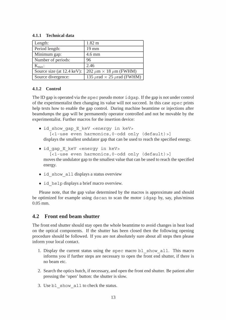
http://www.switch.ch/mail/gw-spec.html#4

http://www.psi.ch/sls/csaxs/beamline-layout

4.1.1 Technical data

Length: 1.82 mPeriod length: 19 mmMinimum gap: 4.6 mmNumber of periods: 96Kmax: 2.46Source size (at 12.4 keV): 202 μm × 18 μm (FWHM)Source divergence: 135 μrad × 25 μrad (FWHM)

4.1.2 Control

The ID gap is operated via the spec pseudo motor idgap. If the gap is not under controlof the experimentalist then changing its value will not succeed. In this case spec printshelp texts how to enable the gap control. During machine beamtime or injections afterbeamdumps the gap will be permanently operator controlled and not be movable by theexperimentalist. Further macros for the insertion device:

• id_show_gap_E_keV <energy in keV>[<1-use even harmonics,0-odd only (default)>]

displays the smallest undulator gap that can be used to reach the specified energy.

• id_gap_E_keV <energy in keV>[<1-use even harmonics,0-odd only (default)>]

moves the undulator gap to the smallest value that can be used to reach the specifiedenergy.

• id_show_all displays a status overview

• id_help displays a brief macro overview.

Please note, that the gap value determined by the macros is approximate and shouldbe optimized for example using dscan to scan the motor idgap by, say, plus/minus0.05 mm.

4.2 Front end beam shutter

The front end shutter should stay open the whole beamtime to avoid changes in heat loadon the optical components. If the shutter has been closed then the following openingprocedure should be followed. If you are not absolutely sure about all steps then pleaseinform your local contact.

1. Display the current status using the spec macro bl_show_all. This macroinforms you if further steps are necessary to open the front end shutter, if there isno beam etc.

2. Search the optics hutch, if necessary, and open the front end shutter. Be patient afterpressing the ‘open’ button: the shutter is slow.

3. Use bl_show_all to check the status.

13

See also the macro overview bl_help and section 4.8 for information about the endstation shutter.

4.3 CVD diamond filter

A water cooled CVD diamond filter can be inserted into the ‘white’ beam to absorb lowenergy radiation and reduce thereby the heat load on the monochromator. For all experi-ments so far this filter was inserted in the beam and it must only be operated by the localcontact.

4.4 Slit systems

Five slit systems are permanently installed.


At 12.1 m from the source is a slit system that allows to limit the beam size in the hori-zontal direction. It can for example be used to symmetrize the source size and illuminateoptics like a Fresnel zone plate with a ‘fully coherent’ beam. All other slit systems havefour blades to limit the beam size both in the horizontal and the vertical direction.

In the optics hutch there is one water-cooled white-beam slit system in front of themonochromator with its center at 25.996 m from the source. The slit blades are watercooled and illuminated under grazing incidence to spread the heat load. The distancebetween the horizontal and vertical slit blades is 145 mm.

The second slit system is the first one for the monochromatic beam. It is locatedbehind the mirror with its center at 30.664 mm from the source. The distance between thehorizontal and vertical slit blades is 20 mm.

In the experimental hutch slits system three and four are installed in the so calledexposure box on the sample table. The maximum opening of these slits is 2.5 mm. Theblades of slit three are made of germanium whereas the blades of slit four are made ofsilicon, both sloped by 10◦ with respect to the x-ray beam. The standard exposure box‘nose’ protrudes 300 mm, a short version 94 mm and a long version 428 mm from the endof the exposure box. The blades of slit system 4 are located 39 and 59 mm upstream fromthe end of the box (133 and 153 mm from the end of the standard nose). The blades ofslit system 3 are located 320 and 340 mm from the end of the box (414 and 434 mm fromthe end of the nose). For both slit 3 and 4 the beam passes first the vertically and then thehorizontally defining blades. The exposure box is motorized along the beam. The positionof the slit systems 3 and 4 relative to the source can be measured using the known sampletable position, see section 4.9.1.

There are two ‘mobile’ slit systems of the JJ X-Ray ESRF type with KF40 flange(http://www.jjxray.dk/-%20at-f7-hv%20%28esrf%29) that can be in-stalled by your local contact, if needed.

4.4.2 Control

There are spec motors for the width and height of the slit opening and for the horizontaland vertical aperture position. Use the spec macro slits_show_all for an overview

14

http://www.jjxray.dk/-%20at-f7-hv%20%28esrf%29

including the motor names as well as slits_help.Your local contact will optimize the slit settings together with you and in general it is

wise to stay with these settings.

4.5 Front end filters

The white-beam filters in front of the monochromator are usually not needed and mustonly be operated by cSAXS staff. See also the macro overview fil_op_help.

The filters in the exposure box are for user operation. See section 4.10 and fil_helpfor further details.

4.6 Monochromator

A liquid nitrogen cooled Si(111) double crystal monochromator defines the energy of thex-ray beam.


The fixed exit Si(111) double crystal monochromator is located at 28.58 m from the source(position of the second crystal). The first crystal is liquid nitrogen cooled. The secondcrystal can be bend for horizontal focusing.

The accessible energy range is from about 4.0 to 18.6 keV. The energy resolution withSi(111) is about ΔE/E ≈ 2 · 10−4. The second monochromator crystal can be used tofocus the beam horizontally by about 10:1 to approximately 20 μm FWHM.

4.6.2 Control

Moving single motors of the monochromator can easily irreversibly damage the mono-chromator. This would be the end of not just your beamtime. Please do not operate themonochromator without introduction from your local contact and without exactly know-ing what to do. To protect you from accidental movements of monochromator componentsare some of these motors password protected. Some monochromator spec macros:

• mono_settings_E_keV <energy in keV>displays the monochromator settings needed for the specified x-ray energy.

• mono_E_keV <energy in keV>moves the monochromator to the settings for the specified energy.

• mono_offs <0-no, 1-yes> controls the usage of empirical theta2 (motormoth2) offsets. In standard operation this feature should be active, see alsosection 4.6.3.

• mono_id <0-no, 1-yes> controls the automatic setting of the ID gap if thex-ray energy is changed. In standard operation this feature should be active, seealso section 4.6.3.

• mono_show_all displays an overview of the monochromator state including thecurrent energy.

15

• mono_help displays a macro overview including the position of all monochroma-tor motors and the current x-ray energy.

The rotation of the second crystal needs to be optimized after it has been set usingmono_E_keV, for example using the dscan command to scan moth2 by plus/minus0.010 degree. Due to top-up mode and the stability of the optics is it usually not necessaryto re-optimize the second crystal position during a beamtime of a few days length.

The bender of the second crystal is accessible via the spec motor mobd and has, likemost monochromator motors, no end switches, i.e., can be damaged.

4.6.3 Energy scans

For energy scans the pseudo motor mokev is available. This motor has not all safetyfeatures of the macro mono_E_keV and will therefore refuse to move by larger steps inenergy at low energies, where crystal collision is an issue. The monochronator is not atall optimized for fast energy changes. If you plan to change or even scan the x-ray energythen please inform your local contact in advance.

To ensure the likelihood that the second crystal rotation moth2 is exactly at the Braggangle empirical corrections for the calculated rotation angles can be used. This feature iscontrolled via mono_offs and is active in standard operation.

To ensure that an undulator harmonic is at the current energy automatic ID gap settingshould be activated via mono_id, which is the default setting.

4.7 Mirror

The mirror is used to reject higher harmonics and to focus in the vertical direction.


The center of the plane mirror is located at 29.43 m from the source. The usable area is400 mm long. The central 12 mm wide part of the mirror is uncoated, i.e., the fused silicais exposed to the beam here. Via the horizontal translation one can choose between thisuncoated and 14 mm wide Pt and Rh coated stripes. The mirror can be bend for verticalfocusing.

4.7.2 Control

As the monochromator, the mirror must not be operated by users without introductionfrom the local contact AND explicit permission. To protect you from accidental move-ments of mirror components these motors are password protected. Some mirror specmacros:

• mirr_coat [<SiO2, Rh or Pt>] positions the part of the mirror with thespecified coating in the X-ray beam.

• mirr_show_all displays a status overview including all motor positions, thecurrently selected stripe and incidence angle.

16

• mirr_help displays a macro overview.

The bender is accessible via the spec motor mibd and has, like most mirror motors,no end switches, i.e., can be damaged.

4.8 End station beam shutter

In the compulsory safety training (see section 2.4) and the introduction from your localcontact you learned how to operate the local access control (LAC) system. Additional tothe LAC panel the end station shutter can be closed due to equipment protection systeminterlocks or simply by a software command issued, for example from spec:

• bl_show_all can be used to check the status of the shutter or to investigate whyit can not be opened.

• shclose overrules the LAC panel. The end station shutter can not be opened untila shopen command is given.

• shopen enables opening of the end station sutter via the LAC panel.

The macros shopen and shclose act additional to the LAC panel in a safety-first way.This means, if either the panel or spec say that the shutter should be closed then it willstay closed. To open the shutter it has to be opened from both the panel and from spec.The order does not matter. The panel will not give LED feedback upon pressing the openbutton if the shutter is still disabled via spec. Effectively this all means that the shuttercan be controlled from spec once it has been opened from the LAC panel.

See also the macro overview bl_help and section 4.2 for information about the frontend shutter.

4.9 Optical tables

Three optical tables are installed in the end station hutch ES1: the sample table, an aux-iliary table that is for example used to motorize the detector flight tube entrance windowand a detector table.


The optical tables in the experimental hutch can be moved horizontally and vertically andcan be tilted around the horizontal axis. They are specified for a maxmimum load of500 kg.

By moving the tables one can damage detectors, vent the beamline vacuum for theincoming beam or the detector flight-tube. Please do not operate the tables without in-troduction from your local contact. To protect you from accidental movements all tablemotors are password protected, apart from the vertical motion of the detector table dttryand the horizontal movement of the whole detector bank dettrx. These two motionsare needed to select and position a detector. Please handle them with care.

The sample table is an optical table, 2400 mm along the beam, 1200 mm perpendicularto it. It has a M6 x 25 mm grid of threaded holes and is stationary along the beam. The

17

distance from the table top to the beam position is typically about 500 mm. The mostupstream threaded hole of the table is at about 34.12 m from the source. A so calledexposure box with in-vacuum beam conditioning like two slit systems, section 4.4, filtersfor attenuating the beam, section 4.10, and a fast shutter, section 4.11, is mounted on theoptical table. The beam exits the exposure box through a ‘nose’ with a mica window thatseparates the beamline vacuum from the in-air sample environment. The standard ‘nose’protrudes 94 mm from the end of the exposure box. The default ‘sample environment’consists of about a cubic metre of air to be filled with whatever setup is needed.

The auxiliary table is 900 mm along the beam, 1500 mm perpendicular to it. Alongthe beam it is motorized on rails.

The detector table is 1200 mm along the beam, 1500 mm perpendicular to it. Alldetectors are located on a platform that can be translated horizontally using dettrx.Vertically the detectors can be positioned using the slow translation dttry of the wholedetector table. Along the beam the detector table is motorized on rails.

4.9.2 Control

The spec macro tables_show_all displays an overview.

4.10 Exposure box filters

There are four filter wheels each containing different thicknesses of silicon and germa-nium filters and other calibration materials of different thicknesses. To avoid hardwaredamage the filters must be operated using the following macros rather than directly bymoving the motors:

• fil_find_trans <transmission between 0 and 1>[<energy in keV>] displays a list of filter combinations with transmission

closest to the specified one. If not specified, the current x-ray energy is used bydefault.

• fil_trans [<transmission between 0 and 1>][<energy in keV>]moves the filter wheels to a combination that is closest

to the specified transmission value. Without parameters a help text and the currenttransmission are displayed.

• fil_installed displays the currently installed materials

• fil_comb <4-digit combination>, like fil_comb 1111 can be usedto used to move a certain filter combination in the beam. With this macro calibrationfoils, which are not chosen by fil_trans, can be moved in the beam.

• fil_show_all displays the current filter setting.

• fil_help displays a macro overview.

18

4.11 Exposure box fast shutter

In the exposure box a magnet driven in vacuum fast shutter is installed. It should beswitched on using fshon to avoid radiation damage for both the sample and the detector,which is therefore the default setting:

• fshon enables the automatic opening and closing of the fast shutter and closes thefast shutter

• fshoff disables the automatic opening and closing of the fast shutter

• fshstatus displays if the fast shutter is switched on

• fsh_close_on_error called from within a macro will close the fast shutterupon errors which cancel command execution, even if the automatic fast shutterclosing is switched off. Upon successful macro completion this feature is deacti-vated.

• fsh_on_on_error called from within a macro will activate automatic fast shut-ter opening and closing and close the fast shutter upon errors which cancel com-mand execution. Upon successful macro completion this feature is deactivated, i.e.,the status of the automatic fast shutter opening and closing remains unchanged.

• fshdelay <delay time in seconds> should not be adjusted by users.See the discussion below.

• fshutter_help displays a command overview.

In scans without motor movements or with the movement of very fast motors likepiezos is the time between closing and re-opening of the fast shutter very short. In thatcase the fast shutter becomes unreliable and it does not make sense to open and close it foreach exposure rather than keeping it open all the time. To disable and re-enable the fastshutter automatically for such cases the following logic has been implemented in spec.Prerequisite is, that the automatic opening and closing of the fast shutter is switched onusing fshon.

The first point of a scan is measured with opening and closing of the fast shutter. Whenthe exposure for the second point shall be taken it is measured, how long the shutter hasbeen closed. If this time is below the threshold defined via fshdelay then the fastshutter closing is delayed for the rest of the scan. By delaying rather than disabling thefast shutter it is ensured, that for example in a two motor scan with a fast first axis anda very slow second axis the fast shutter will still be closed when the slow second axis ismoved.

Please do not change the timing of this automatically enabled delayed-closing featurewithout discussion with your local contact.

4.12 Hexapod

A PI M850.11 Hexapod is available. It emulates three degrees of translation and threedegrees of rotation around a user-defined center of rotation. Its main purpose is the po-sitioning of heavy equipment with micron precision. A smaller Hexapod M810 is forexample used for positioning optical elements.

19


Please see the separate description inhttp://www.psi.ch/sls/csaxs/ManualsEN/PI_Hexapod_M850p11_cSAXS.pdf for the large HexapodM850 andhttp://www.psi.ch/sls/csaxs/ManualsEN/PI_Hexapod_M810_Datasheet.pdf for the smaller M810.

4.12.2 Control

The Hexapod related macros in spec need the internal number of the Hexapod that isaddressed by issuing a command. The big M850 has the number 1 and the small M810number 2.

After connecting the Hexapod and switching on the controller an initialization has tobe performed using hex_ini. Please make sure that its save for the Hexapod to move inany direction since software limits will be ignored at this point.

• hex_ini initializes the controller, includes a search for the home position whileignoring software limits

• hex_off disables the Hexapod motors in spec. The Hexapod motors are thennot listed by wa

• hex_on enables the Hexapod motors in spec. hex_ini executes this automati-cally.

• hex_set_pivot_point defines the center of rotation

• hex_show_pivot_point displays the current center of rotation

• hex_help displays a command overview

4.13 Air bearing rotation stage

A Micos UPR160F air bearing rotation stage is available upon request. It is for examplepart of the standard 3D setup for Ptychography and STXM, see alsohttp://www.psi.ch/sls/csaxs/endstations.

• upr_ini initializes the controller. This macro must be executed after switchingon the controller, prior to using the stage in spec.

• upr_on enables the rotation stage for its use in spec.

• upr_off disables the rotation stage for its use in spec.

• upr_speed <speed in deg/sec> can be used to set the rotation speed.

• upr_show_all displays a status overview

• upr_help displays a brief macro overview

20

http://www.psi.ch/sls/csaxs/ManualsEN/PI_Hexapod_M850p11_cSAXS.pdf

http://www.psi.ch/sls/csaxs/ManualsEN/PI_Hexapod_M810_Datasheet.pdf


4.14 Piezo

A PI E710 piezo controller is available upon request. It is for example part of the standard2D and 3D setups for Ptychography and STXM, see alsohttp://www.psi.ch/sls/csaxs/endstations.

4.14.1 Macros

Some of the features of the E-710 piezo controller that go beyond the simple use as a po-sitioning device have been implemented in spec. For continuous scans, see section 3.10,or any other standard experiment one has not to deal directly with the macros below:

• pz_on activates all E-710 controlled piezo motors for use in spec. Upon errorsthe piezo motors may become deactivated and this command can be used to re-activate them.

• pz_off deactivates all E-710 controlled piezo motors for use in spec. This isuseful to avoid error messages if the controller is switched off but the piezo motorsare still configured in spec.

• pz_auto_zero <motor> recalibrates the zero position for the specified piezoaxis. This should be performed after the controller has been switched on. Typicallyit will be defined in the controller setup that all connected axes are zeroed uponstartup and manual zeroing via this macro will not be necessary.

• pz_wait_settledown <0-off, 1-on> If active, spec waits after motormovements until the controller signals that the piezo is settled at its destinationposition. This feature being active is the default.

• pz_version display the controller version

• pz_status <motor> displays the (error) status of the specified axis

• pz_stop <motor> stops all wave generators of the controller for the speci-fied axis. This macro should for example be used after starting a wave form withpz_run_waveform.

• pz_velocity <motor> [<velocity in mm/sec>] set and display thevelocity for the specified axis. Typical values are very high like 12.5 mm/sec.

• pz_def_ramp <motor> <amplitude in mm> <time in seconds>defines a waveform that ramps up linearly by the specified amplitude and back thesame amplitude and rate plus intermediate sections as connections. The total timeneeded for the complete waveform is specified as parameter, i.e., this routine makesit easier to define the repeat frequency rather than the ramp speed.

• pz_show_single_waveform <motor> [<output sampling>]display the measured waveform. Prerequisite is the definition of a wave form, forexample using pz_def_ramp. An output sampling greater than 1 can be used tosuppress screen output of values to increase the speed of the screen output.

21


• pz_run_waveform <motor> [<no. of repeats,0 for infinity or 1-...>]

runs a previously defined waveform.

• pz_step_response <motor> <step size in mm>[<no. of points to report>]

moves the specified axis by the specified step size (in mm) and records the positionas a function of time. These data are read by spec and stored as a scan file. Atleast 500 points should be used for the report table to see the step, depending on thecurrent speed settings.

• pz_report_table <motor> <no. of points to report>[<output sampling>] [<start index>]

reads the report table of the piezo controller and stores the data as a scan file. Allspecified points are read but specifying a sample larger than 1 can be used to skippoints for output to the screen and data file. The report table is for example filledusing the pz_step_response or the pz_def_ramp macro.

• pz_show_all displays a status overview

• pz_help displays a macro overview

4.15 Detector flight tube lengths

Two detector flight tubes are available. The short flight tube is 2063 mm long, the longone 7000 mm. This is the nominal distance from the entrance window to the exit windowposition. The entrance window is a thin sheet of mica, separating the flight tube vacuumof a few mbar from the surrounding air. The exit window is made of a 350 μm thick Mylarfoil and has a clear aperture of 400 mm. A reduction flange to 120 mm clear aperture isavailable and adds 21.1 mm to the flight-tube length. This smaller diameter can be usedwith a 75 μm Kapton window. A 13 μm Kapton window of 600 mm diameter is availablefor flushing the flight tube with helium. The flight tube can be moved along the beamwhich allows to move its entrance close to the sample position. The total detector tosample distance should be measured at least. Ideally one measures a calibration samplewith known spacings like the 58.380 A of silver behenate:http://www.esrf.eu/UsersAndScience/Experiments/CRG/BM26/SaxsWaxs/Silverbehenate.

4.16 Light curtain

In front of the detector table a light curtain is installed. If it is triggered then detector andauxiliary table motors are blocked in low level hardware. The effect is like triggered endswitches. Some motions are blocked completely, others only in one direction. One canfo example move the detector table away from the auxiliary table but not closer whichallows to disentangle these two systems once the light curtain is triggered.

If the light curtain is triggered then:

• Enter the hutch and investigate the problem.

• Carefully resolve the problem by moving motors with spec.

22

http://www.esrf.eu/UsersAndScience/Experiments/CRG/BM26/SaxsWaxs/Silverbehenate

4.17 PILATUS detector

The PILATUS 2M detector is the standard detector at the cSAXS beamline. A PILATUS300k-W is available, for example as wide angle detector. A single 100k PILATUS modulemay be available upon request.

Several publications are describing PILATUS technology like, e.g., B. Henrich, A.Bergamaschi, C. Bronnimann, R. Dinapoli, E. F. Eikenberry, I. Johnson, M. Kobas, P.Kraft, A. Mozzanica, and B. Schmitt, PILATUS: A single photon counting detector forx-ray applications, Nucl. Instrum. Methods Phys. Res. A 607 247-249 (2009).


The PILATUS 2M detector has 1475 × 1679 pixels of 172 × 172 μm2 resulting in an ac-tive area of 253.7 × 288.8 mm. It consists of 3 × 8 detector modules of 487 × 195 pixelseach. The area between the modules is not sensitive to x-rays and appears as simulated‘dead’ pixels in the data frames, i.e., only 92 % of the 2.48 million pixels are real pixels,the other 8 % are simulated dead pixels between the modules. The horizontal separationof modules is seven and the vertical one 17 pixels.

The PILATUS 300k-W has 195×1475 pixels. It consists of three modules in arow. See also http://dectris.com/sites/pilatus300k-w.html. The sin-gle module 100k has 487×195 pixels.

If the count rate in a pixel reaches 220 = 1048576 then the counter wraps over to 0and continues counting. The detector is radiation tolerant but not radiation hard. It cannot withstand the intensity of the direct beam. Long exposure to high intensity will alterthe sensitivity of the exposed area.

The distance from the front surface of the detector housing to the surface of the detec-tor modules is 20 mm.

Related information:

• PILATUS 2M on the DECTRIS web pages:http://www.dectris.com/sites/pilatus2m.html

• PILATUS pages of the SLS detector group:http://pilatus.web.psi.ch/pilatus.htm

• Effect of low, medium and high gain settings on the dead time:http://pilatus.web.psi.ch/DATA/REPORTS/rate_scans.html.See also the discussion in section 4.17.6.

• energy threshold, see section 4.17.6

4.17.2 Control

Make sure that the detector is protected from the direct beam before opening the shutterfor the experimental station.

23

http://dectris.com/sites/pilatus300k-w.html

http://www.dectris.com/sites/pilatus2m.html

http://pilatus.web.psi.ch/pilatus.htm

http://pilatus.web.psi.ch/DATA/REPORTS/rate_scans.html

4.17.3 Macro overview

The data directories are handled by general macros, see section 3.7.All PILATUS detector macros except pilatus_show_all need as the first param-

eter the detector number. The 2M detector is number 1, the 300k-W number 2, and thesingle 100k module is number 3.

• pilatus_on <det.no.> enables a PILATUS detector for use in spec. BothPILATUS detectors can be run in parallel.

• pilatus_off <det.no.> disables a PILATUS detector for use in spec.

• pilatus_basename <det.no.> <base name> sets the first part of theimage filenames.

• pilatus_file_format <det.no.> <base name> sets the file format toeither uncompressed edf or byte-offset compressed cbf.

• pilatus_threshold <det.no.> <"full" or "partial">[<threshold in keV>] [<1-low, 2-medium, 3-high gain>]

sets the energy threshold for detection, see section 4.17.6.

• pilatus_show_all displays a status overview

• pilatus_help displays a command overview

4.17.4 Region of interest

The PILATUS 2M can be configured to be read out in

• eight banks (3 × 8 modules, i.e., full frame)

• four banks (3 × 4 modules)

• eight modules (2 × 4 modules)

• two banks (3 × 2 modules)

• two modules (1 × 2 modules)

mode. Switching between these modes is relatively fast but can NOT be done from specin an automated way, see section 4.17.5. Further region of interest features are currentlynot available.

4.17.5 Startup and shutdown procedure

The PILATUS 2M detector has to be started by your local contact according to the fol-lowing procedure:

1. Switch on the Julabo chiller for the detector. Start it by pressing its enter button forseveral seconds. The temperature set-point is 23◦C.

24

2. Switch on the power supply at the back side of the detector.

3. Log on to the detector PC: ssh -X det@x12sa-pd-1.

4. On the detector PC mount the file server via automount:cd /sls/X12SA/Data10

5. Still on the detector PC start camserver from its directory:cd ˜/p2_8bank./camonly_8b. Wait until the camserver startup procedure is finished and a’*’ prompt is displayed.

6. Activate use of the detector in spec using pilatus_on 1.

7. With the monochromator at the correct energy startpilatus_threshold 1 "full"in spec. See also section 4.17.6.

8. You may define the base directory relative to the user home directory usingpilatus_basedir and print an overview using pilatus_show_all.

9. If readout of less than the full frame is needed then perform additionally the follow-ing steps:

• Switch the PILATUS detector off in spec using pilatus_off 1

• exit camserver

• On the detector PC run one of the following, from ˜/p2_8bank:

– ./camonly_8b (3x8 modules, full frame)

– ./camonly_4b (3x4 modules)

– ./camonly_8m (2x4 modules, center - left)

– ./camonly_2b (3x2 modules, center)

– ./camonly_2m (1x2 modules, center)

Modules are specified horizontally × vertically.

• Enable the PILATUS detector in spec using pilatus_on 1

• Call pilatus_threshold 1 "partial" in spec. The calibration canonly be done for the full detector and is still active (if you did it before, asdescribed above). The dead time correction is reset upon starting the sub-detector camserver version but activated again by pilatus_thresholdwith the "partial" parameter.

4.17.6 Threshold

The PILATUS detector has energy threshold and gain settings. The default setting for theenergy threshold is 55% of the x-ray energy for high counting efficiency but still no crosstalk between neighbouring pixels. The threshold can be raised for example to suppressfluorescence from the sample.

25

The default gain setting is low gain for the highest count rates with a dead time of about124.7 ns, see http://pilatus.web.psi.ch/DATA/REPORTS/rate_scans.html.At medium gain the dead time is about 200.4 ns and at high gain it is 338.8 ns. The lowerthe energy the higher the gain needed. At lower energies also energy threshold settingshigher than 55 % of the current x-ray energy are needed. Otherwise the detector startscounting noise. This will be evident from an exposure without beam, if it happens. Largerareas of such hot pixels due to too low energy threshold will draw a high current andeventually damage the detector. The minimum threshold is currently 3.5 keV for highgain settings.

The spec macro pilatus_threshold can be called with only the detector num-ber and "full" as parameters to use default settings. For user defined settings the energythreshold can be given as third command-line argument and the gain as fourth argument:’1’ for low gain (high count rates), ’2’ for medium gain and ’3’ for high gain (low countrates). The PILATUS control program camserver may decide on its own to change theenergy threshold setting. One should always check the settings that are really applied, forexample, using pilatus_show_all.

If not the full detector is read out, see section 4.17.5, then the energy threshold mustbe set first for the full detector using the "full" parameter and then for the sub-detectorreadout using the "partial" parameter. This is just a workaround: The energy thresh-old calibration can currently only be performed with the full detector. The sub detectorcamserver versions do not change the previously set threshold upon startup but unfortu-nately these versions do not report the previously applied threshold. Furthermore, thedead time correction has to be set in camserver after starting the sub-detector version.This is done by pilatus_threshold with the "partial" parameter. Additionallya warning in spec is switched off and the last known threshold setting is reported as thecurrent one. If spec is restarted inbetween then these last known values are deleted andone must start with the full detector again to avoid useless warning messages.

4.18 Cyberstar scintillation point detector

The Cyberstar detector is often used as a kind of monitor, looking at air-scattering orsample back-scattering, or as point detector for photon correlation spectroscopy. It isavailable as counter in spec, typically as a channel called mon. Macros for setting thehigh voltage, gain and energy window are currently not available. If such macros areneeded then please discuss this with your local contact well in advance.

4.19 Flat single APD

An APD of 10 mm × 10 mm active area and 200 μm thickness mounted in a flat housingis available upon request. It is an APD0008 from FMB Oxford. It is controlled via theAPD counter electronics NIM module ACE. The ACE module is connected via RS232 tospec. For a mcaro overview see ace_help.

26

http://pilatus.web.psi.ch/DATA/REPORTS/rate_scans.html

4.20 Amptek XR-100CR detector and PX4 pulse processing unit

The Amptek XR-100CR is a two-stage Peltier cooled Si PIN diode used as energy dis-persive detector. It is connected to the PX4 digital pulse processing unit. Additionally tothe slow read out of full spectra, the PX4 unit has the option to integrate up to eight en-ergy ranges and provides the resulting signals as TTL output that can be fed into a specaccessible counter card. The dynamic range of the detector is quite limited and its activearea is 6 mm2 small. The active area is 500 μm thick.

The PX4 unit is interfaced to spec via a serial RS232 connection. Currently it isassumed that the spec serial interface number 3 is connected to the PX4 unit and config-ured as 57600 baud, no parity, raw mode.

4.20.1 Maro overview

The data directories are handled by general macros, see section 3.7.

• px4_config <config. no.> loads a configuration to the controller. Cur-rently the configuration 1, the factory default for high energy resolution, the con-figuration 2 with shorter peaking time for higher count rates, and configuration 3for even higher count rates with even worse energy resolution are available. Con-figuration 4 is for a different detector head with 25 mm2 sensor, not available at thebeamline. This macro must be used first to initialize the PX4 unit.

• px4_gain [<gain 3.1 - 703>] sets the analog gain.

• px4_peaking_time [<time in micro sec.>] sets the peaking time inmicro seconds.

• px4_autotune should be run after loading a new configuration or after changingparameters like gain or peaking time. The lower threshold for the discriminationof slow channel events, the lower threshold for the discrimination of fast channelevents and the input voltage offset added to the pre-amplifier output are determinedautomatically.

• px4_scaler_threshold [<scaler no.> <threshold low><threshold high>] sets the integration range in channels for the specified

scaler output.

• px4_scaler_enabled <scaler no.> <enabled 0-no, 1-yes>enables or disables the output of the integrated scaler signal.

• px4_count starts a continuous data acquisition.

• px4_plot [<log-y 0-no, 1-yes>] reads and plots the current spectrum.

• px4_set_basedir <relative directory> sets the data directory rela-tive to ˜/Data10/px4/. The directory is automatically created.

• px4_set_basename <first part of the filename>defines the fixed part of the file name for the energy spectra.

27

• px4_on <level> defines how the energy dispersive detector is used in spec:

0. deactivates automatic use of the PX4 unit

1. activates automatic use but without readout of spectra, i.e., only the scalerchannels are used.

2. activates full use of the unit including automatic read-out and storage of theenergy spectra.

• px4_off deactivates the energy dispersive detector for automatic use in spec.

• px4_show_config displays the current configuration.

• px4_show_status displays the current status variables.

• px4_show_all displays both configuration and status.

• px4_help displays a macro overview.

4.20.2 Startup procedure

Connect the detector head to the PX4 unit, this unit to the fan-out box and this box tottyS3 of the spec PC. In spec start px4_config 2, check px4_show_statusuntil the detector head temperature is not printed in bold face anymore, i.e., reached 230 K.Without X-rays on the detector start px4_autotune to set the thresholds for the sup-pression of noise. Switch the detector on for usage in spec using px4_on 2 and recorda spectrum using ct. The spectrum can be displayed with the spec online plot and theMatlab macro image_spec, see section 5. If the total number of counts in certain rangesof channels should be output as TTL pulses then use px4_scaler_threshold to de-fine the ranges and px4_scaler_enabled to enable the outputs. The outputs maybe connected to the multi channel scaler for continuous scans, see section 4.21, or to thespec counter card accessible via the black fan-out box in the back-top of the rack.

4.21 Multi channel scaler (MCS)

A multi channel scaler can be used to count TTL pulses, for example output by the Amptekenergy dispersive detector, see section 4.20, in a burst scan or continuous scan.

Currently up to 31 input signals can be connected to the inputs 2-31. Input 1 is con-nected internally to the 50 Mhz timebase and must not be used. The control input 1 shouldbe connected to the PILATUS trigger output. For each input channel currently up to 8192values can be stored, i.e., this value defines the maximum number of exposures in a burst,see section 3.9, or continuous scan, see section 3.10.

4.21.1 Macro overview

The data directories are handled by general macros, see section 3.7.

• mcs_trigger should be left at the automatic setting. In this mode the MCS istriggered either by the PILATUS detector or by spec, if the PILATUS is not activeor not used in burst mode.

28

• mcs_basename [<fixed part of filename>] may be used to set thefirst part of the data file names

• mcs_on activates the MCS for use in spec

• mcs_off deactivates the MCS for use in spec

• mcs_show_all displays a status overview

• mcs_help displays a macro overview

4.22 X-ray eye and similar cameras

An x-ray eye is available at the beamline. It consists of a 100 μm YAG scintillator thatis monitored by a CCD camera using a 10× microscope lens. The camera has a lowdynamic range and therefore its gain must be adapted to the incident illumination eithermanually or automatically. The following spec macros all need as the first parameter thespec-internal number of the serial interface over which the camera is connected. For thex-ray eye this is usually 0, 9 or 10.

• cam_manual_gain <interf.no.> [<gain 0-8>] switches to manualgain mode and sets the gain

• cam_shutter_speed <interf.no.> switches to auto light control and setsthe speed of the electronic shutter. This can be used to reduce the intensity if theminimum manual gain of 0 is not sufficient for this.

• cam_senseup <interf.no.> [<0-off, 1-12 for 2x to 128x>]on-sensor integration

• cam_zoom <interf.no.> [<-1-off, 0-8>]provides an electronic zoom feature

• cam_hmirr <interf.no.> [<0-off, 1-on>] mirror images horizon-tally

• cam_vmirr <interf.no.> [<0-off, 1-on>] mirror images vertically

• cam_show_all <interf.no.> displays a status overview

• cam_help displays a command overview including here unlisted options for titledisplay etc.

4.23 Fingerlakes Instrumentation ProLine CCD

A ProLine PL1001E CCD with Kodak KAF-1001E class 1 sensor, 1024 × pixels, maybe available upon request. It can be connected via USB 2.0 to the spec PC. Please seefli_help for an overview on the available macros.

29

4.24 Analog and digital I/O

Analog -10 to 10 V input (ADC) and output (DAC), TTL (5 V) input and output and optocoupler input and output (24 V maximum) connections are available in the experimentalhutch. If you need any of these then please discuss this with your local contact beforeyour beamtime. The following spec macros are provided to control these IO channels:

• ttl_out <ch.no.> [<0 or 1>] optionally sets and displays the state of thespecified output channel

• ttl_out_auto <ch.no.> [<value while counting>] controls au-tomatic setting of the output channel. If a value of 0 or 1 is specified then theoutput channel is brought to this state before the counting starts and reset to theinverse state afterwards. This feature is deactivated with a negative value.

• ttl_in <ch.no.> displays the state of the specified input channel.

• ttl_show_all displays the status of all input and output channels and of theautomatic output channel setting.

• opt_out <ch.no.> [<0 or 1>] optionally sets and displays the state of thespecified output channel

• opt_out_auto <ch.no.> [<value while counting>] controls au-tomatic setting of the output channel. If a value of 0 or 1 is specified then theoutput channel is brought to this state before the counting starts and reset to theinverse state afterwards. This feature is deactivated with a negative value.

• opt_in <ch.no.> displays the state of the specified input channel.

• opt_show_all displays the status of all input and output channels and of theautomatic output channel setting.

• dac_out <ch.no.> [<voltage in V>] optionally sets and displays thestate of the specified output channel

• adc_in <ch.no.> displays the voltage at the specified input channel.

• adcdac_show_all displays the status of all analog input and output channels.

• io_show_all displays the status of all digital and analog input and output chan-nels and their automatic setting.

• io_wait [<time in seconds>] optionally sets and displays the wait timethat is applied after all automatic IO channels are set before the counting starts. Thiswait time is for example needed by the fast shutter. It is not applied if no automaticchannel setting is active.

• io_help displays a macro overview

The automatic TTL output is for example used for triggering the in-vacuum fast shutterthat is installed in the exposure box.

30

4.24.1 DAC pseudo motor

The -10 to +10 V output of the digital to analog converters can be controlled via a pseudomotor in spec. This can be used for controlling a device via an analog voltage. Examplesare power supplies and analog piezo controllers. If you need such a feature then pleasearrange this with your local contact and see dac_mot_help in spec.

4.25 Digital delay generators

Two Stanford Research Systems digital delay generators DG645 are available. Each haseight channels. Please see ddg_help for an overview over the available macros.

4.26 Temperature controller

A LakeShore 336 temperature controller is available upon request. Please see ls_helpfor an overview over the available macros.

4.27 Teslameter

A Group3 DTM-133 digital teslameter may be available upon request. It is connected viaGPIB to the spec PC. A pseudo counter can be defined for reading the field strength.Please see dtm_help for an overview on the available macros.

4.28 Syringe pumps

4.28.1 Cetoni neMESYS syringe pumps

Three neMESYS syringe pumps are available at the beamline upon request. One pumpis connected to the spec PC x12sa-rack-1 via an RS232 interface and the otherpumps are daisy chained using a CAN bus. On the control PC a server program is runningindependently of spec to optionally run programs in parallel to command execution inspec.

4.28.1.1 Technical data The neMESYS OEM module has a minimum velocity of59.26 nm/s and a maximum velocity of 5.93 mm/s. The pulsation free minimum ve-locity is approximately twenty times the minimum velocity. The smallest step is 35 nm.The maximum force is 290 N. The stroke is 62 mm. The maximum syringe diameter is30 mm. The pulsation free minimum and the maximum flow rate are for a 0.5 μl/60mmsyringe 10 pl/s - 49 nl/s, for a 100 μl/60mm syringe 2 nl/s - 10 μl/s, and for a 25 ml/60mmsyringe 500 nl/s - 2.5 ml/s. PEEK valves with FFKM/FFPM sealing are available. Theyhave an internal volume of 45 μl and are suitable for a temperature range from 0 - 50◦C, apressure of up to 2 bar on the syringe and up to 0.5 bar on the experiment side. The valveshave an UNF 1/4”-28 connection.

31

4.28.1.2 Macro overview After your local contact has connected the pumps they needto be initialized using nem_init and a following nem_home for the calibration of thezero position is recommended. Then one can run the pumps using nem_... macros orvia pseudo motors and/or counters set up by your local contact.

Movements can be combined to programs that are stored and run on the syringe serverprogram, independent of spec.

The spec macros for these pumps are:

• nem_init initializes the connection to syringe pump

• nem_calibration controls the syringe dependent mm/μl calibration

• nem_velocity controls the default syringe velocity

• nem_home performs a home movement to calibrate the position

• nem_off closes the connection to the server program

• nem_valve_input moves the valve to its input position. It can not be checkedif a valve is connected and successfully moving.

• nem_valve_outputmoves the valve to its output position It can not be checkedif a valve is connected and successfully moving.

• nem_pos displays the current position

• nem_start_move_abs starts moving to an absolute position without waitingfor the completion of the movement

• nem_move_absmoves to an absolute position, waits until the syringe pump stops

• nem_start_move_rel starts moving relative to the current position withoutwaiting for the completion of the movement

• nem_move_rel moves relative to the current position

• nem_dose moves permanently

• nem_prog selects the active program for programming

• nem_cmd sends a program string

• nem_delete_last_cmd deletes the last command from a program

• nem_delete_prog deletes an entire program

• nem_display_programs displays all programs on the server

• nem_exec executes a program on the server

• nem_pause programs a delay

• nem_wait_stop waits until the syringe motor stops

32

• nem_mot_wait controls macro motor and counter wait behavior

• nem_cancel stops all pumps immediately

• nem_stop programs a pump stop

• nem_show_all displays a status overview

• nem_help displays a macro overview

4.28.2 Hamilton syringe pumps PSD/4

The PSD/4 syringe pumps from Hamilton are not available at the beamline. But if youbring such a pump with RS232 interface then the spec interface for controlling the pumpis available. These pumps can be daisy-chained, i.e., only one RS232 connection to thespec PC is needed for controlling several pumps.

After your local contact has connected the pumps they need to be initialized usinghsp_init_out_right or hsp_init_out_left. Then one can run the pumpsusing hsp_...macros or via pseudo motors and/or counters set up by your local contact.The spec macros for these pumps are:

• hsp_init_out_right initialize syringe and valve, output position is right

• hsp_init_out_left initialize syringe and valve, output position is left

• hsp_wait controls macro motor and counter wait behavior

• hsp_calibration controls the steps/μl calibration

• hsp_velocity controls the syringe velocity

• hsp_backlash controls the backlash correction

• hsp_valve_inputmoves the valve to its input position

• hsp_valve_outputmoves the valve to its output position

• hsp_valve_bypassmoves the valve to its bypass position

• hsp_start_move_abs starts moving to an absolute position without waitinguntil this position is reached

• hsp_move_abs moves to an absolute position

• hsp_start_move_rel starts moving relative to the current position withoutwaiting until this position is reached

• hsp_move_rel move relative to the current position

• hsp_pos display the current position

• hsp_prg_begin starts the programming of a command string

33

• hsp_prg_wait programs a wait time

• hsp_prg_end ends programming a command sequence

• hsp_prg_cmd sets directly the command string

• hsp_prg_exec executes a pre-programmed command sequence

• hsp_show_all displays status overview for the specified pump

• hsp_help displays a macro overview

4.29 EPICS interface

Much of the hardware access is controlled via EPICS, transparent to the user. The fol-lowing macros for interaction with EPICS are for use by the local contact rather thanusers:

• epics_dump_motor_par displays the parameter of all EPICS motors that areconfigured in spec.

• epics_holding_current <motor> [<0-off, 1-on>] optionally setsand displays the holding current setting for the specified motor. A new setting be-comes active once the motor is moved and is lost upon reboot of the correspondingVME crate. Enabling holding current may damage a motor.

• epics_holding_current_show_all displays the holding current settingfor all motors that are configured in spec.

• epics_reset_m1 resets position and limit for all EPICS_M1 motors. This willonly be useful in the initial phase of a beamtime when all motors are set up. Themacro displays which motor positions are reset and with which command sequencethis can be set back to the previous settings. This allows setting back a few selectedmotors using copy-paste.

• epics_dump_encoder_par displays the EPICS encoder settings

• epics_set_encoder_offset <encoder no.> <offset value>sets the offset parameter The setting is lost upon reboot of the VME crate.

• epics_set_encoder_dir <encoder no.> <dir. +1 or -1>sets the direction parameter. The setting is lost upon reboot of the VME crate.

• epics_boottime displays the boot time of all known VME crates.

• epics_load displays the CPU load for the IOCs on the beamline VME crates.As a rule of thumb the load should not exceed 60 %.

• epics_help displays a macro overview

34

4.30 Julabo closed cycle water chillers

Integration of the sample table and detector chiller are planned. Please ask your localcontact about the current status.

4.31 Oxford cryojet

Integration of the cryojet is planned. Please ask your local contact about the current status.

4.32 Lambda Genesys power supplies

Two 0-40 V, 0-19 A and one 0-60 V, 0-12.5 A power supplies are available. They can becontrolled via their RS232 interface. Pseudo motors and counters can be defined in specby your local contact to control voltage and current. See lgen_help for an overview.As startup procedure lgen_init or lgen_init_cc is needed to initialize the device.

5 Matlab (plotting and analysis)

Your local contact will provide some Matlab routines including a simple online viewer for2D data, read and write functions for the data and macros for azimuthal integration. Atthe beamline the Matlab routines can be found in the directory ˜/Data10/matlab/of your e-account. From time to time we update the online available version athttp://www.psi.ch/sls/csaxs/software.

The macros accept ’Name’,value pairs for optional parameters. Calling the macroswithout parameters will display in most cases a help text and an example. Usually macroswill accept parameters of sub-macros. An example is the online viewer image_specthat accepts the parameters of image_read and image_show since it is calling thesefunctions to read and display the data.

Some of the Matlab functions:

• image_read can be used for reading PILATUS cbf and edf and other data files.

• image_show is a macro for reading and displaying an image data file.

• image_spec is an online viewer for spec, see section 5.1

• spec_read can be used to access the spec data file

• spec_plot can be used to plot data from the spec data file

• scan_movie can be used to view a whole scan or for writing this display as avideo in AVI format.

• prep_valid_mask tries to identify the valid, i.e., neither dark nor hot pixels.

• display_valid_mask visualizes a valid pixel mask

• beamstop_mask cuts out the beamstop, i.e., a user specified region, from the listof valid pixels.

35

http://www.psi.ch/sls/csaxs/software

• tune_valid_mask can be used to remove remainig hot pixels by comparingmedian filtered integrated to raw data

• get_beam_center can be used to optimize the beam center in a 7 × 7 gridaround the specified good guess with sub-pixel precision. This macro is not veryfast.

• prep_integ_masks is used to prepare the radial integration of SAXS data.

• display_integ_masks visualizes integration masks

• radial_integ performs the radial integration of SAXS data using the integra-tion masks prepared beforehand.

• integrate_range integrates a range of scans as they become available

• plot_radial_integ can be used to display radially integrated data

• mcs_mesh displays multi channel scaler (MCS) data, see section 4.21 for detailson the MCS

• stxm_online is a viewer for scanning x-ray transmission microscopy (STXM)like raster scans

5.1 Online viewer

The Matlab online viewer for 2D detector data is typically started from a text-only Matlabsession running on x12sa-cn-1. This text session typically runs in the second or thirdsub-window of the main text console (spec running in the first sub-window).

To start it from scratch log on to the compute node using ssh -X x12sa-cn-1.On the compute node change to the Matlab directory cd ˜/Data10/matlab and startmatlab -nodesktop. In Matlab start image_spec. The macro will display a briefhelp on its parameters. For displaying PILATUS 2M data with the default options useimage_spec(1);

5.2 Example: how to get azimuthally integrated data

There are more options available than it is useful to list here. The following exampledemonstrates how one can get to integrated intensities, a common task in small-anglex-ray scattering (SAXS).

5.2.1 Valid pixel mask

To create a list of all valid pixels, called valid pixel mask, you should record a seriesof at least ten exposures of an unstructured intensity distribution for two well separateddetector positions. Glassy carbon or air scattering may be options. One starts the macroonce to create a new valid pixel mask for the first exposure series. This mask will notcontain some of the pixels close to the beam stop since they have been sorted out due tohigh intensity variations. Calling the macro again for the second series of exposures with

36

the Extend parameter set to "or" will update the mask with the valid pixels from thesecond series and thereby add the beam-stop region to the valid pixels:

prep_valid_mask(’˜/Data10/pilatus/S05000-05999/S05716/’);prep_valid_mask(’˜/Data10/pilatus/S05000-05999/S05717/’, ...’Extend’,’or’);

The valid pixel mask is stored in ˜/Data10/analysis/data/ if nothing else hasbeen specified.

5.2.2 Including the beamstop in the valid pixel mask

The function beamstop_mask can be used to cut out the beamstop and its support fromthe valid pixel mask. The user needs to specify the name of an example data image andthe (x,y,) coordinates of the beamstop area. The example image is displayed with the user-defined beamstop area in reduced intensity to aid judging if the coordinates are sufficient.If the result is satisfying then the updated mask can be saved by setting the ’SaveData’parameter to 1:

beamstop_mask([’˜/Data10/pilatus/S05000-05999/S05715/’ ...’e12612_1_05715_00000_00000.cbf’], ...

’xyCoord’,[705 0; 712 619;715 699;720 699; 720 619;721 0], ...’SaveData’,1);

The original valid pixel mask will be overwritten.

5.2.3 Determining the beam center

Using silver behenate or any other stromg scatterer one can determine the beam centerby minimizing the standard deviation of the intensity integrated over a ring as a functionof the ring center position. One needs to specify the name of the data file, a good guessfor the beam center position and the radius range for the ring over which the macro willintegrate:

get_beam_center([’˜/Data10/pilatus/S05000-05999/S05715/’ ...e12612_1_05715_00000_00000.cbf’], ...

’GuessX’,717,’GuessY’,708,’RadiusFrom’,80,’RadiusTo’,100);

It is not recommend to increase the area over which this macro searches for the optimumbeam center beyond the default value of ±3 pixels since this macro is quite slow. Thebeam center that is returned has usually sub pixel precision.

5.2.4 Preparing the integration masks

The coordinates for the azimuthal integration are determined once and stored in a data file.As parameters one needs to specify the name of a raw data file for the final quality controldisplay and the beam center as for example determined using get_beam_center:

prep_integ_masks([’˜/Data10/pilatus/S05000-05999/S05715/’ ...’e12612_1_05715_00000_00000.cbf’], ...[ 716.901 707.951 ],’NoOfSegments’,16);

37

The number of azimuthal segments is by default 1. If the SAXS data exhibit azimuthalasymmetry then this may be captured by integrated in a certain number of segments like 16in the present case. The integration masks are stored in ˜/Data10/analysis/data/if nothing else has been specified.

5.2.5 Integrating a range of scans

Azzimuthal integration of data can be done using radial_integ. To integrate a rangeof scans as they become available a wrapper function is available:

integrate_range(5714,5915);

This call integrates the scans 5714 up to and including 5915. Without further parametersthe default input path ˜/Data10/pilatus/... is used and the default output path˜/Data10/analysis/radial_integration/ for the integrated data in Matlabdata format. The integrated data of all files of a scan are stored in a single data file. Thefile name is deduced from the name of the first file of raw data that is read and integrated.

5.2.6 Plotting radially integrated data

By default the plotting routine displays the mean of all points, i.e., of all integrated inten-sities stored in a file and also of all azimuthal segments:

plot_radial_integ([’˜/Data10/analysis/data/’ ...’radial_integration/’ ...’e12612_1_05714_00000_00000_integ.mat’]);

This plotting function returns the plotted data, i.e., it can be used for simple averagingtasks.

5.2.7 Removing hot pixels from the valid pixel mask

If one notices that the azimuthal integration has artificial spikes then these are most likelyrelated to hot pixels that have not been recognized so far. One can mask them by com-paring the median filtered azimuthally integrated data against the raw data, if the raw dataexhibit a smooth intensity distribution:

tune_valid_mask(’˜/Data10/pilatus/S05000-05999/S05720/’, ...’SaveData’,1);

In the present example all *.cbf files from the specified PILATUS directory are com-pared against the radially integrated data stored under the default name in the defaultlocation. A quality control plot is dispolayed and if the result is satisfying then one canset the ’SaveData’ parameter to 1 to update the stored valid pixel mask. For this updatedmask to take effect the integration masks need to be generated again, see section 5.2.4.

38

5.2.8 Determining the sample to detector distance using silver behenate

If one records the SAXS signal of silver behenate, integrates the data and determines theposition of a ring of intensity by clicking on the plot displayed by the plotting function, seesection 5.2.6, then one can calculate the sample to detector distance as r·0.172mm/ tan(n·arcsin(λ/(2 ·58.380A)) ·2) which may be approximated by r ·0.172mm ·58.380A/(n ·λ).Here r is the radius of the ring of intenisty in pixels, n is the order of the silver behenatediffraction ring and λ is the x-ray wave length as displayed by mono_show_all inspec. The detector pixel size of 0.172 mm and the silver behenate spacing of 58.380 Aare the remaining parameters.

6 Chemistry lab.

A small chemistry lab is located directly at the beamline to help you preparing your sam-ples for the measurements. The lab is not suitable for handling, e.g., ultra toxic or ra-dioactive hazards. Among others the following equipment is available:

• solvent cabinet (with exhaust)

• fume hood: width 1.5 m, max. 500 m3/h, nitrogen and argon gas supply upon re-quest

• horizontal laminar flow box as local cleanroom environment (in the user preparationroom, not in the chemistry lab): Skanair HFX90, 0.9 m width

• fridge freezer combination with not too much space: Dometic ML305C, fridge setto 5◦C, freezer to -20◦C, min. -35◦C possible

• Millipore Milli-Q Gradient water purification

• stereo microscope Zeiss Stemi 2000 with Schott KL1500 LCD cold light source(the latter with ring light adapter and alternatively double goose neck light guide)

• Leica DM2500 M high resolution microscope with camera and sample positionencoder attached (in the user preparation room, not in the chemistry lab)

• Hettich Universal 320R centrifuge, relative centrifugal force up to 21382, tempera-ture set point between -20◦C and 40◦C.

• heating cabinet: SalvisLab TC100, inner dimensions 450×500×460 mm3 / 100 luseable volume, max. 200◦C, microprocessor PID control

• digital RTD thermometer

• pH meter VWR sympHony SB70P

• pH indicator paper, pH 1-14

• three weighing machines for different weight ranges: Sartorius BL210S with 0.1 mgreading and max. 200g, max. 4 kg and max. 50 kg weighing machines

39

• ultrasonic bath without heating option: Merck Eurolab, 35 kHZ

• small magnetic stirrer

• magnetic stirrer and heating plate combination: IKA RCT basic, max. 1100 RPMand 250◦C

• heating plate with digital control and external sensor option: Torrey Pines ScientificHP 30A-2, max. 400◦C

• small membrane pump

• desiccators for vacuum or drying pad use

• hotmelt glue gun

• glassware washer

• demin. water and standard cold water from the tap

• Eppendorf safe lock tubes in 0.5 and 1.5 ml

• Eppendorf pipettes: Reference, 20, 100, 200 and 1000 ml

• basic glassware, spattles, tweezers, scalpels, syringes

• glass capillaries with 10 μm wall thickness, capillary wax and wax pen

Suggestions for improvements are welcome. Please report missing or almost out of stockitems. Please arrange with your local contact if you need excessive amounts of certainconsumables.

7 Troubleshooting / Frequently Asked Questions

• Is the beam shutter open?Why can’t I open the beam shutter?Is there beam available for the beamlines at all?Please use bl_show_all in spec.

• How do I get help? Please contact your local contact using the PSI phone numberfrom http://www.psi.ch/sls/csaxs/people

or http://www.psi.ch/sls/csaxs/contactsor the mobile phone number 079 343 92 30 that is printed on the phone at thebeamline as well. From within PSI dial a 0 first to get out. If this fails try to contactsomebody else from the cSAXS staff page. You can phone the accelerator controlroom (5503) any time and briefly describe your problem. The control room has aphone list and will contact the appropriate person if needed.

40

http://www.psi.ch/sls/csaxs/people

http://www.psi.ch/sls/csaxs/contacts

• The Matlab online viewer crashed or beeps when I move the mouse over it orI can not zoom in anymore. What shall I do?Search for the Matlab window. Typically this is in the main console window thesecond or third tabulator (the first being spec). Stop the online viewer thereusing <CTRL>-<C>. Close the online viewer plot window using the mouse orclose all in Matlab. Restart the online viewer image_spec by pressing<Cursor Up> to get the previous command starting with image_spec and con-firm with return. See also section 5.1.

41

A History

March 18th 2011 Oliver Bunk v1.02, include slit 0, small Hexapod, PILATUS300k-W, and indications of other pieces of hard-ware like teslameter, digitial delay generators,temperature controller, Leica microscope, up-date links to new web page

June 17th 2010 Oliver Bunk v1.01, include Cetoni and Hamilton syringepumps, minor updates

May 21st 2010 Oliver Bunk v1.00, include an example for azimuthal inte-gration using Matlab and other minor updates

November 26th 2008 Oliver Bunk v0.80, update x-ray energy rangeSeptember 23rd 2008 Oliver Bunk v0.29, new name epics_boottime,

document pon, poff and pkill, document newSMS features, update pilatus_threshold

August 7th 2008 Oliver Bunk v0.28, new names id_gap_E_keV,mono_settings_E_keV, mono_E_keV,new macros mono_offs, mono_id, dmesh,section on continuous scans cont_line andcont_mesh, SMS features, delayed shutterclosing, E-710 piezo controller macros

June 3rd 2008 Oliver Bunk v0.27, add distance to PILATUS modulesMay 28th 2008 Oliver Bunk v0.26, add power socket and user bike informa-

tionMay 26th 2008 Oliver Bunk v0.25, add light curtain and slit 1 and 2 position,

combine beamline layout with control sectionMay 23rd 2008 Oliver Bunk v0.24, add information on the location of slit 3

and 4 and the sample tableMay 19th 2008 Oliver Bunk v0.23, add section on the beamline layout and

sub-section on the beamline web pages, start thetroubleshooting section

May 2nd 2008 Oliver Bunk v0.22, rename pilatus_set_thresholdand pilatus_set_basename,add pilatus_file_format,add Mythen macros,add basic chemistry lab. inventory

April 17th 2008 Oliver Bunk v0.21, update data transfer section, add rsyncfor Windows

April 13th 2008 Oliver Bunk v0.20, major updateDecember 12th 2007 Oliver Bunk v0.17, last of several updates including among

other Hexapod, fast shutter, exposure box slitsand filters, PILATUS burst mode, camera andMatlab macro informations

August 23rd 2007 Oliver Bunk include PILATUS threshold informationAugust 19th 2007 Oliver Bunk several minor updatesAugust 8-9th 2007 Oliver Bunk first draft

42

B Phone list

The up to date phone-list is available online athttp://www.psi.ch/sls/csaxs/contacts. A printout can be found on the white-board in the control room.

C Guest network

Connecting to the network or using any PSI IT resource requires agreement to the ‘Usageand Monitoring of IT Resources at PSI’ regulations available online athttp://ait.web.psi.ch/regulations/.

An open WLAN is available inside the SLS building and other selected areas. Usingit should be ‘plug and play’.See http://ait.web.psi.ch/services/guest_net/ for details.

Alternatively you may connect your laptop or PC via an ethernet cable to the beamlinenetwork provided

• it is in accordance with the security guidelines of our IT department, including anup-to-date virus scanner

• gets a network address via DHCP

• does not create heavy network load (no streaming of music and videos, IP-basedphone calls etc.)

Your browser must be configured for using a proxy. In Mozilla you may use an automaticproxy configuration via http://nedi.web.psi.ch/proxy.pac (set this link inedit → preferences → advanced → proxy → automatic proxy configuration). Otherwisethe proxy can be set manually to proxy.psi.ch, port 3128.

D Data transfer

The amount of data created depends strongly on the application but please keep in mindthat a single PILATUS frame means 10 MB of data typically compressed to 2.5 MB inCBF format. A typical run of 3-5 days creates between 100 GB and 15 TB. The data willcompress well using tar+gzip which is the default for data transfer to user disks at cSAXS.Please bring a sufficient amount of sufficiently large USB or eSATA disks for your data.The data will be transferred using a ‘media station’ running Linux for transfer to ext3 orNTFS formated disks. We recommend that the data transfer is set up by your localcontact and started while you measure, well before the end of your beamtime.

D.1 File systems

The disks will be formated at the beamline or must be preformated in either ext2 (Linux),ext3 (Linux), or NTFS (Windows). FAT32 is rather limited in the number of files perdirectory and the maximum file size and therefore not suitable for data transfer.

43

http://www.psi.ch/sls/csaxs/contacts

http://ait.web.psi.ch/regulations/

http://ait.web.psi.ch/services/guest_net/

http://nedi.web.psi.ch/proxy.pac

D.2 Data transfer

Ideally you choose an ext3 or ext2 file system. Using FAT32 usually ends with runninginto one of its limitations, see section D.1. Meanwhile NTFS is sufficiently supportedunder Linux to be used as well.

D.2.1 Mounting drives

When an external hard-disk is connected then a popup window asks what to do. If youwant to access a formated disk then mount it via this popup. The drive will appear under/media/. If you want to format the disk then cancel this popup dialog.

If the auto mounting does not work follow the instructions athttps://intranet.psi.ch/Controls_IT/LinuxMediaStationUsage#manual_mount. These instruc-tions are only available within the PSI network and need authentification with a PSI ac-count.

D.2.2 Formating drives under Linux

A not mounted drive can be formated using sudo gparted. This tools allows for-mating the system partitions as well, i.e., be sure what you do or you may crash thesystem unrecoverable. Select the external disk in the list top-right. Most likely it is/dev/sdb. It is NOT /dev/sda or /dev/md0. If partitions of the external drive aremounted then unmount them using ‘Partition’, ‘Unmount’. If you want to completelyerase all partitions and start from scratch with a new partition table then select ‘Device’,‘Set Disklabel’.

Clicking on the unallocated disk space you can add a ‘New’ partition to it. Thispending operation needs to be confirmed using ‘Apply’.

Mounting the drive can be done endng gparted, unplugging and plugging in thecable to the external drive and selecting ‘Open’ in the then emerging pop-up window.

D.2.3 Access rights for pre-formated Linux drives

If the e-account has not sufficient acces rights to an ext2 or ext3 drive thensudo usbdisk777 will flatten the access rights for all disks mounted as sub-directories of /media/.

D.2.4 Compressing data

The PILATUS data will usually compress very well. A tar-bzip2 job for compressing thedata could be run on x12sa-cn-1. Your local contact can start˜/Data10/bin/tar_pilatus_as_availableto compress data in bunches of a certain number of scans. At the end of the beamtimeyour local contact could run˜/Data10/bin/tar_pilatus_last and˜/Data10/bin/tar_non_pilatus_and_tar_filesfor compressing the remaining data. You can read gzip compressed tar archive underWindows using helper applications like 7-Zip.

44

https://intranet.psi.ch/Controls_IT/LinuxMediaStationUsage#manual_mount

D.2.5 Transferring data using rsync

Your local contact can start the script ˜/Data10/bin/rsync_usbdisk for you. Thedata transfer should be started at the beginning of the beamtime to run in parallel to theacquisition.

D.2.6 Related informations

The mounted disks do not appear in /etc/fstab. The free space can be checked usingdf -h.

A sudo umount command for manual unmounting of disks is available, e.g.,sudo umount /media/disk. Using sudo gparted and the ‘Partition’ menuwith the ‘Unmount’ option is possible as well.

D.3 Windows specific information

D.3.1 Formating drives

Either you need a local contact with sufficient access rights for the Windows PC or youhave to prepare the hard disk on another PC or laptop where you have an account withsufficient acces rights. . On this machine the computer management should be startedfrom the administrative tools menu or by running compmgmt.msc /s. Select ‘DiskManagement’ and format the external disk to NTFS. Afterwards you can select ‘proper-ties’ of this partition by right clicking on it and set under security sufficient access rights.Typically this means ‘Modify’ and related access right for ‘Everyone’.

D.3.2 Mounting the e-account on the file server

Mount your e-account using the explorer: ‘Tools’, ‘Map Network Drive’, folder\\x12sa\e-account (replace with your e-account name), do not ‘Reconnect at lo-gon’, ’Connect using a different user name’ (your e-account and password), ‘Finish’.

E Where to eat

The ’personnel restaurant’ Oase offers lunch from 11:30 until 13:30 and dinner from17:00 until 20:00, both Monday to Friday.See http://services.web.psi.ch/oase/menu.php for the menu.

The cafeteria west, the ‘timeout’ is open from 8:00 - 16:00, Monday to Friday, seehttp://log.web.psi.ch/verpflegungsbetriebe/oeffnungszeiten.shtml

for the up-to-date opening hours. Outside opening hours vending machines are available.In Villigen, 10 minutes walk from PSI, you will find

• the restaurant ‘Zum Hirschen’ (closed on Tuesdays)

• a baker, Monday to Friday 6:30-12:00 and 15:00-18:00, Saturday 7:00-13:00

• a small Volg supermarket, Monday to Friday 7:30–18:30, Saturday 7:30-16:00

45

http://services.web.psi.ch/oase/menu.php

http://log.web.psi.ch/verpflegungsbetriebe/oeffnungszeiten.shtml

• and an ATP machine.

Towards Wurenlingen is a large COOP supermarket easily reachable by bike.By bus and car several restaurants in Brugg, Baden, Bottstein, Wurenlingen etc. can

be reached.

F Public transport

Public transport in Switzerland is excellent. Even at PSI frequently buses are calling.Check for connections from and to ‘Villigen PSI West’ on the SBB home-page:http://www.sbb.ch/en/index.htm.

There are direct connections by train form Zurich airport to Brugg. From Brugg onecan take the bus to get to PSI.

46

http://www.sbb.ch/en/index.htm

Indexa2scan (spec), 8access rights, Linux (data transfer), 44access rights, Windows (data transfer), 45ADC inputs, 30adc_in, 30adcdac_show_all (spec), 30air bearing rotation stage, 20analog IO, 30APD, 26area scan (spec), 9area scan, continuous (spec), 9ascan (spec), 8

badge, 4beam energy, 15beamstop_mask (Matlab), 35bicycles, 5bikes, 5bl_show_all (spec), 17bl_show_all (spec, open front end shutter), 13burst_at_each_point, 10burst_scan (spec), 10bzip2 (data transfer), 44

cameracam_help (spec), 29cam_hmirr (spec), 29cam_manual_gain (spec), 29cam_senseup (spec), 29cam_show_all (spec), 29cam_shutter_speed (spec), 29cam_vmirr (spec), 29cam_zoom (spec), 29title display, 29

cameras (spec interfaced), 29Cetoni syringe pumps, 31chemistry lab., 39chillers (spec), 35close end station shutter (spec), 17closed cycle chillers (spec), 35compressing data (data transfer), 44compute node, 6computer based safety training, 5cont_line (spec), 9cont_mesh (spec), 9continuous area scan (spec), 9continuous line scan (spec), 9cryojet, 35cSAXS_help (spec), 7ct (spec), 9ct_save (spec), 9CVD diamond filter, 14Cyberstar detector, 26

d2scan (spec), 9DAC outputs, 30DAC pseiudo motor, 31dac_out (spec), 30data directories (spec), 7data file (spec), 7data storage, 6data transfer, 43delay generators, 31detector flight tube, 22detector to sample distance, 22DG645 digital delay generator, 31digital delay generators, 31digital IO, 30digital user office, 4dir_base (spec), 7dir_grouping, 7dir_help, 8dir_scan_no, 7, 8dir_show_all, 8display_integ_masks (Matlab), 36display_valid_mask (Matlab), 35dmesh (spec), 9dosimeter, 4double crystal monochromator, 15dscan (spec), 8DTM-133 teslameter, 31DUO, 4

e-account, 6empirical monochromator theta2 offsets, 15end station shutter, 17energy threshold, PILATUS, 25EPICS (spec), 34epics_dump_encoder_par (spec), 34epics_dump_motor_par (spec), 34epics_help (spec), 34epics_holding_current (spec), 34epics_holding_current_show_all (spec), 34epics_load (spec), 34epics_reset_m1 (spec), 34epics_set_encoder_dir (spec), 34epics_set_encoder_offset (spec), 34epics_show_boottime (spec), 34ES1 shutter, 17exposure box filters, 18exposure box: length of nose, 14

FAQ, 40fast shutter, 19

help, 19on, off (spec), 19status (spec), 19

47

trigger, 30fil_comb (spec), 18fil_find_trans (spec), 18fil_help (spec), 18fil_installed (spec), 18fil_op_help (spec), 15fil_show_all (spec), 18fil_trans (spec), 18file server, 6file systems (data transfer), 43filter, CVD diamond in front end, 14filters (optics hutch), 15filters, exposure box, 18flat single APD, 26flight tube length, 22focusing, horizontal (monochromator), 15focusing, vertical (mirror), 16formating drives, Linux (data transfer), 44formating drives, Windows (data transfer), 45front end shutter, 13fsh_close_on_error, 19fsh_on_on_error, 19fshdelay, 19fshoff (spec), 19fshon (spec), 19fshstatus (spec), 19fshutter_help (spec), 19

gain, PILATUS, 25gap (insertion device), 12get_beam_center (Matlab), 36Group3 teslameter, 31guest bicycles, 5guest house reservation, 5

Hamilton syringe pumps, 33hex_help (spec), 20hex_ini (spec), 20hex_off (spec), 20hex_on (spec), 20hex_set_pivot_point (spec), 20hex_show_pivot_point (spec), 20Hexapod, 19

help, 20initialize (spec), 20pivot point (spec), 20

higher harmonic rejection (mirror), 16horizontal focusing (monochromator), 15hsp_backlash (spec), 33hsp_calibration (spec), 33hsp_help (spec), 34hsp_init_out_left (spec), 33hsp_init_out_right (spec), 33hsp_move_abs (spec), 33hsp_move_rel (spec), 33hsp_pos (spec), 33

hsp_prg_begin (spec), 33hsp_prg_cmd (spec), 34hsp_prg_end (spec), 34hsp_prg_exec (spec), 34hsp_prg_wait (spec), 34hsp_show_all (spec), 34hsp_start_move_abs (spec), 33hsp_start_move_rel (spec), 33hsp_valve_bypass (spec), 33hsp_valve_input (spec), 33hsp_valve_output (spec), 33hsp_velocity (spec), 33hsp_wait (spec), 33

I/O, analog and digital, 30ID gap, setting automatically, 15id_gap_E_keV, 13id_help, 13id_show_all, 13id_show_gap_E_keV, 13image_read (Matlab), 35image_show (Matlab), 35input output, analog and digital, 30insertion device, 12integrate_range (Matlab), 36integration masks (Matlab), 36io_help, 30io_show_all (spec), 30io_wait (spec), 30

Julabo chillers, 35

laboratory, 39LakeShore 336 temperature controller, 31light curtain, 22line scan (spec), 8line scan, continuous (spec), 9log file (spec), 7long flight tube, 22loopscan (spec), 9

M810 Hexapod, 19M850.11 Hexapod, 19Matlab macros, 35Matlab online viewer, troublshooting, 41MCS, 28mcs_basename (spec), 29mcs_help (spec), 29mcs_off (spec), 29mcs_on (spec), 29mcs_show_all (spec), 29mcs_trigger (spec), 28mcs_mesh (Matlab), 36mesh (spec), 9Micos air bearing rotation stage, 20mirr_coat, 16

48

mirr_help (spec), 17mirr_show_all (spec), 16mirror, 16mirror to source distance, 16mokev (spec), 16mono_E_keV (spec), 15mono_help (spec), 16mono_id (spec), 15, 16mono_offs (spec), 15, 16mono_settings_E_keV (spec), 15mono_show_all (spec), 15monochromator, 15

automatic ID gap setting, 15empirical theta2 offsets, 15energy scans, 16mokev, 16set energy, 15

monochromator to source distance, 15mount e-account, Windows (data transfer), 45mounting drives, Linux (data transfer), 44multexp_ctimes (spec), 9multi channel scaler, 28multiple exposures in standard scans (spec), 9

nem_calibration (spec), 32nem_cancel (spec), 33nem_cmd (spec), 32nem_delete_last_cmd (spec), 32nem_delete_prg (spec), 32nem_display_programs (spec), 32nem_dose (spec), 32nem_exec (spec), 32nem_help (spec), 33nem_home (spec), 32nem_init (spec), 32nem_mot_wait (spec), 33nem_move_abs (spec), 32nem_move_rel (spec), 32nem_off (spec), 32nem_pause (spec), 32nem_pos (spec), 32nem_prog (spec), 32nem_show_all (spec), 33nem_start_move_abs (spec), 32nem_start_move_rel (spec), 32nem_stop (spec), 33nem_valve_input (spec), 32nem_valve_output (spec), 32nem_velocity (spec), 32nem_wait_stop (spec), 32neMESYS syringe pumps, 31new_std_files (spec), 7number cruncher, 6

online viewer (Matlab), 36online viewer, troublshooting, 41

open end station shutter (spec), 17opt_in, 30opt_out (spec), 30opt_out_auto (spec), 30opt_show_all (spec), 30optical tables, 17opto coupler IO, 30Oxford cryojet, 35

phone numbers, 43PI E710, 21PI M810 Hexapod, 19PI M850.11 Hexapod, 19piezo controller, 21PILATUS

active area, 23distance to modules, 23dynamic range, 23energy threshold, 25pilatus_threshold (spec), 24, 25pilatus_basename (spec), 24pilatus_file_format (spec), 24pilatus_off (spec), 24pilatus_on (spec), 24pilatus_show_all (spec), 24pixel size, 23region of interest, 24ROI, 24startup, 24

PILATUS 2M detector, 23pkill (spec), 10plot_radial_integ (Matlab), 36poff (spec), 10point detectors, 26pon (spec), 10power sockets, 5prep_integ_masks (Matlab), 36prep_valid_mask (Matlab), 35printing from spec (pon, poff), 10PSD/4 syringe pumps, 33px4_autotune (spec), 27px4_config (spec), 27px4_count (spec), 27px4_gain (spec), 27px4_help (spec), 28px4_off (spec), 28px4_on (spec), 28px4_peaking_time (spec), 27px4_plot (spec), 27px4_scaler_enabled (spec), 27px4_scaler_threshold (spec), 27px4_set_basedir (spec), 27px4_set_basename (spec), 27px4_show_all (spec), 28px4_show_config (spec), 28px4_show_status (spec), 28

49

pz_auto_zero (spec), 21pz_def_ramp (spec), 21pz_help (spec), 22pz_off (spec), 21pz_on (spec), 21pz_report_table (spec), 22pz_run_waveform (spec), 22pz_show_all (spec), 22pz_show_single_waveform (spec), 21pz_status (spec), 21pz_step_response (spec), 22pz_stop (spec), 21pz_velocity (spec), 21pz_version (spec), 21pz_wait_settledown (spec), 21

radial integration (Matlab), 36radial_integ (Matlab), 36region of interest, PILATUS, 24relative scan (spec), 8ROI, PILATUS, 24round_scan (spec), 9

safety training, 5sample to detector distance, 22sample to detector distance (silver behenate), 39scan motor (spec), 8scan_movie (Matlab), 35shclose (spec), 17shopen (spec), 17short flight tube, 22shutter (fast), 19shutter, end station, 17shutter, front end, 13silver behenate, 22, 39slit locations, 14slit to source distance, 14slits_help (spec), 14SMS notification (spec), 12sms_beam_back, 12sms_error (spec), 12sms_help (spec), 12sms_no_beam, 12sms_numbers (spec), 12sms_send() (spec), 12sms_show_all (spec), 12sms_wait_for_beam, 12sockets (power), 5spec commands, 8spec data file, 7spec help, 7spec log file, 7spec startup, 7SRI digital delay generators, 31Stanford Research Systems digital delay generators,

31

stop motor (spec), 8stxm_online (Matlab), 36surveillance cameras (spec interfaced), 29syringe pumps (Cetoni), 31syringe pumps (Hamilton), 33

tables_show_all (spec), 17tar (data transfer), 44temperatur controller, 31teslameter, 31timescan (spec), 9troubleshooting, 40TTL IO, 30ttl_in, 30ttl_out (spec), 30ttl_out_auto (spec), 30ttl_show_all (spec), 30tune_valid_mask (Matlab), 36tw (spec), 10twc (spec), 10tweak motor position (spec), 10

U19 undulator, 12umv (spec), 8umvr (spec), 8undulator, 12UPR160F, 20upr_help, 20upr_ini (spec), 20upr_off (spec), 20upr_on (spec), 20upr_speed (spec), 20upr_show\verb-.all (spec), 20

valid pixel mask (Matlab), 35, 36vertical focusing (mirror), 16

wa (spec), 8wm (spec), 8

x-ray beam energy, 15x-ray eye, 29x12sa-cn-1, 6x12sa-cn-2, 6x12sa-cn-3, 6x12sa-comp-1, 6x12sa-comp-2, 6x12sa-cons-1, 6x12sa-rack-1, 7

50

csaxs notes v1.02 (march 18th, 2011) - paul scherrer institute · csaxs notes v1.02 (march 18th,...

Documents