csc 213 lecture 12: quick sort & radix/bucket sort
TRANSCRIPT

CSC 213
Lecture 12:Quick Sort & Radix/Bucket Sort

Quick-Sort (§ 10.2)Quick-sort is another divide-and-conquer sorting algorithm: Divide: pick an
element x (the pivot) and split into 2 partitions: L -- elements less than
x G -- elements equal to
or bigger than x Recur: sort L and G Conquer: merge L, x
and G
x
x
L G
x

DividePartitioning is slightly more comple than merge-sort:
In turn, remove each element y from S
Compare y and pivot. Insert y into L or G depending on comparison result
Only insert and remove first/last elements, so each insertion and removal takes O(1) time
Partitioning takes
_______ time
Algorithm partition(S, C, pivot)while S.isEmpty()
y S.removeFirst()comp = C.compare(y, pivot)if comp < 0
L.insertLast(y)else // e.g., comp > 0
G.insertLast(y)return L, pivot, G

Execution TreeCan depict execution using binary tree Node still represent recursive quick-sort calls
Left side shows initial sequence and highlights pivot Right side shows final (sorted) sequence
Root node is the initial call Leaves show base cases -- calls of size 0 or 1
7 4 9 6 2 2 4 6 7 9
4 2 2 4 7 9 7 9
2 2 9 9

7 2 9 4 3 7 6 1 1 2 3 4 6 7 8 9
Execution Example
7 2 9 4 3 7 6 1 1 2 3 4 6 7 8 9
First, select a pivot

Execution ExamplePartition, recurse and select that pivot
2 4 3 1 2 4 7 9
7 2 9 4 3 7 6 1 1 2 3 4 6 7 8 9
2 4 3 1 2 4 7 9

Execution ExamplePartition, recurse and enjoy the base case
2 4 3 1 2 4 7
1 1
7 2 9 4 3 7 6 1 1 2 3 4 6 7 8 9

Execution Example
Recursive call to sort the G partition
2 4 3 1 1 2 3 4
1 1 4 3 3 4
9 9 4 4
7 2 9 4 3 7 6 1 1 2 3 4 6 7 8 9
4 3 3 4
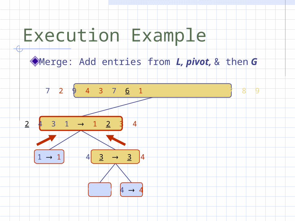
Execution ExampleMerge: Add entries from L, pivot, & then G
2 4 3 1 1 2 3 4
1 1 4 3 3 4
9 9 4 4
7 2 9 4 3 7 6 1 1 2 3 4 6 7 8 9

Execution Example
7 9 7 1 1 3 8 62 4 3 1 1 2 3 4
1 1 4 3 3 4
9 9 4 4
Recursively solve G partition
7 2 9 4 3 7 6 1 1 2 3 4 6 7 8 9
7 9 7 1 1 3 8 6

Execution ExampleRecursive calls and handle the base case
7 9 7 1 1 3 8 6
8 8
2 4 3 1 1 2 3 4
1 1 4 3 3 4
9 9 4 4
7 2 9 4 3 7 6 1 1 2 3 4 6 7 8 9
7 9 7 9
9 9 9 9

Execution Example
8 8
2 4 3 1 1 2 3 4
1 1 4 3 3 4
9 9 4 4
7 2 9 4 3 7 6 1 1 2 3 4 6 7 8 9
7 9 7 1 1 7 7 9
Merge: Add entries from L, pivot, & then G
7 9 7 9
9 9 9 9
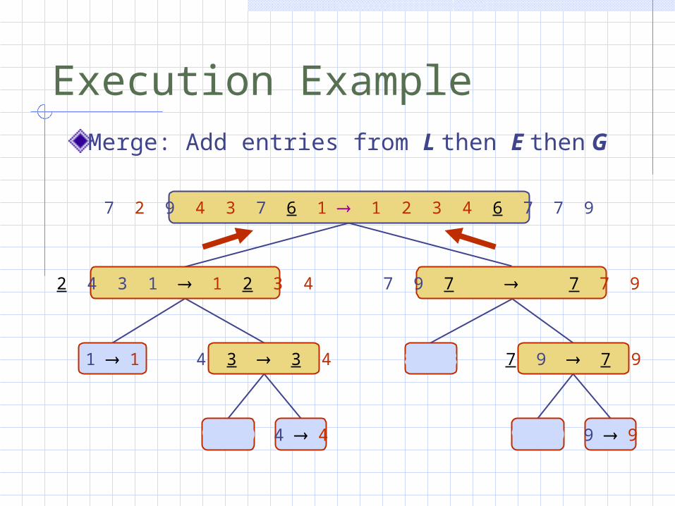
Execution ExampleMerge: Add entries from L then E then G
8 8
2 4 3 1 1 2 3 4
1 1 4 3 3 4
9 9 4 4
7 2 9 4 3 7 6 1 1 2 3 4 6 7 7 9
7 9 7 1 1 7 7 9
7 9 7 9
9 9 9 9

Worst-case Running TimeWorst possible case for quick-sort: we keep pivoting around the minimum or maximum elements
Either L or G will have size n 1 and the other has size 0Big-Oh Running time is therefore equal to the sum
n (n 1) … 2 Total running time is therefore ____________
depth time
0 n
1 n 1
… …
n 1 1
…

Quick-Sort Pivot
In theory, any Entry can be the pivot Algorithm only requires there be one
In reality, want median Entry as pivot Traditionally used first or last Entry This means data already sorted or in
reverse order is the worst case Also fairly common cases. Oops, our Bad.
Now usually select an Entry at random

Expected Running Time
7 9 7 1 1
7 2 9 4 3 7 6 1 9
2 4 3 1 7 2 9 4 3 7 61
7 2 9 4 3 7 6 1
Good call Bad call
Good pivotsBad pivots Bad pivots
1 2 3 4 5 6 7 8 9 10 11 12 13 14 15 16

Expected Running Time
Toss coin 2n times to get n heads on averageFor node at depth i, we can expect i/2 ancestors were good calls Input sequence would be at most n*(¾)i/2
Expect nodes at depth 2* log4/3 n to be leaves Expected tree height = O(2*log n) = O(log n)
Process nearly all of the original entries at each depth
Expected running time of quick-sort is ______

We Can Rebuild Her…Of previous sorts, only Bubble-sort does not use additional data structures Selection-sort & Insertion-sort can
use a Sequence-based priority queue Heap-sort can use a heap-based priority
queue (though this can be avoided) Merge-sort uses additional Sequences
We can modify Quick-sort to run in-place

In-Place Quick-SortDuring partitioning, rearrange entries in the sequence such that: entries smaller than pivot (e.g., L) have
rank less than l pivot has rank between l entries larger than pivot (e.g., G) have
rank greater than l
First partition S into L and G and then move pivot in between these partitions

In-Place Partitioning
3 2 5 1 0 7 3 5 9 2 7 9 8 9 7 6 9
j k
Algorithm inPlacePartition(Sequence S, int j, int k, Entry pivot) while j < k do
while C.compare(S.elemAtRank(j), pivot) < 0 do j j + 1 while j < k and C.compare(S.elemAtRank(k), pivot) ≥ 0 do
k k – 1 if (j < k) then
S.swapElement(j, k) // j contains the rank of the first element in G
3 2 5 1 0 2 3 5 9 7 7 9 8 9 7 6 9
j kjk

In-Place Quick-SortAlgorithm inPlaceQuickSort(Sequence S, int lower, int upper)
if lower < upper theni select a new pivot rank between lower and upperpivot S.elemAtRank(i)
remove pivot from Sh inPlacePartition(S, lower, upper-1, pivot)inPlaceQuickSort(S, lower, h - 1)inPlaceQuickSort(S, h, upper)
S.insertAtRank(h, pivot) else // If lower == upper, we only have 1 Entry to sort // If lower > upper, then no Entries to sort. // So these are our base cases; we do not have to do anything! endif

Summary of Sorting Algorithms
Algorithm Time Notes
selection-sort O(n2) uses priority queue slow (good for small
inputs)
insertion-sort O(n2) uses priority queue slow (good for small
inputs)
quick-sortexpected O(n log n)
in-place, randomized fastest (good for large
inputs)
heap-sort O(n log n) uses additional heap fast (good for large inputs)
merge-sort O(n log n) sequential data access fast (good for huge
inputs)

Can We Do Better?
Comparing entries to another we cannot do better than O(n log n) time We will talk more about this in a week
But what if we had a sort that did not do not actually compare the entries Any ideas (from non-BIF400 students)
how this would work?

Bucket-Sort (§ 10.4.1)
Bucket-sort maintains auxiliary array, B, of Sequences (e.g., buckets)Bucket-sort sorts a Sequence, S, based upon the entry’s key: Phase 1: Move each entry in S to the end
of bucket B[k], where k is the entry’s key Phase 2: For i 0, …, B.size()-1, move
entries in bucket B[i] to end of sequence S

Bucket-Sort ExampleSuppose keys range from [0, 9]
7, d 1, c 3, a 7, g 3, b 7, e
1, c 3, a 3, b 7, d 7, g 7, e
Phase 1
Phase 2
0 1 2 3 4 5 6 8 9
B
1, c 7, d 7, g3, b3, a 7, e
S
7
S

Bucket-Sort AlgorithmAlgorithm bucketSort(Sequence S, Comparator c)
B new Sequence[c.getMaxKey()] // instantiate the Sequence at each index within B
while S.isEmpty() do // Phase 1entry S.removeFirst()B[c.compare(entry, null)].insertLast(entry)
for i 0 to B.length - 1 // Phase 2while B[i].isEmpty() do
entry B[i].removeFirst()S.insertLast(entry)
return S

Bucket-Sort Properties
Keys are indices into an array Must be non-negative integers and not
arbitrary objects Does not need a Comparator
Stable Sort Preserves relative ordering of two entries
with same key Bubble-sort and Merge-sort can also be
stable

Bucket-Sort Extensions
Extend Bucket-sort with Comparator Specifies maximum number of buckets compare(key, null) returns index to which a key
is mapped
For Integer keys in range a – b: Comparator maps key k to k – a
For Boolean keys, Comparator returns: index of 0 if key is false index of 1 if key is true

Bucket-Sort Extensions
Can actually use Bucket-sort with any keys who can must be from some bounded set, D, of values E.g., D could be U.S. states, molecular
structures, people I want to kill, … Comparator must have rank for each value
in D E.g., Rank states in alphabetical order or order
of admission Ranks then serve as the indicies

d-Tuples
d-tuple is combination of d keys (k1, k2, …, kd) ki is the “i-th dimension of the tuple”
Example: Points on a plane are a 2-tuple X-axis is 1st dimension, Y-axis is 2nd
dimension

Lexicographic Order
Lexicographic order of d-tuples is defined recursively as:
(x1, x2, …, xd) (y1, y2, …, yd)
x1 y1 (x1 y1 (x2, …, xd) (y2, …, yd))
How would we order following tuples?(3, 4) (7, 8) (3, 2) (1, 4) (4, 8)
(1, 4) (3, 2) (3, 4) (4, 8) (7, 8)

Lexicographic Sorting
Arranges d-tuples by making d calls to a stable sorting algorithm E.g., One call to sort each tuple
dimension
Concept lexicographicSort(Sequence s, Comparator c, Sort stableSort)
for i c.size() downto 1stableSort.sort(s, c, i)
return s

Lexicographic Sorting Example
Example:(7,4,6) (5,1,5) (2,4,6) (2, 1, 4) (3, 2, 4)

Lexicographic Sorting Example
Example:(7,4,6) (5,1,5) (2,4,6) (2,1,4) (3,2,4)
(2,1,4) (3,2,4) (5,1,5) (7,4,6) (2,4,6)
(2,1,4) (5,1,5) (3,2,4) (7,4,6) (2,4,6)
(2,1,4) (2,4,6) (3,2,4) (5,1,5) (7,4,6)

Radix-Sort (§ 10.4.2)
Radix-sort is a lexicographical sort that uses Bucket-sort as its stable sorting algorithmRadix-sort is applicable to tuples where the keys in each dimension i can be made into indexes in the range [0, N-1] Note: Integers are keys that can be
considered to have multiple dimensions Pass i as compare’s second parameter

Radix-Sort for Integers
Can represent integer as a b-tuple of digits or bits:
62 = 1111102 04 = 0001002
Decimal representation uses need 10 buckets Binary numbers need 2 buckets
Radix-sort algorithm runs in O(bn) time For 32-bit integers b = 32 Radix-sort sort Sequences using integer
keys in O(32n) time

Radix-Sort for IntegersAlgorithm binaryRadixSort(Sequence S, Comparator c)
for i 0 to 31bucketSort(S, 2, i, c)
return S
If key is an int, the value of the ith bit of an integer is:
((key >> i) & 1)

ExampleSorting a sequence of 4-bit integers
1001
0010
1101
0001
1110
0010
1110
1001
1101
0001
1001
1101
0001
0010
1110
1001
0001
0010
1101
1110
0001
0010
1001
1101
1110

Daily Quiz
Always selecting the first entry as the pivot, show the execution tree for Quick-sort when sorting the following in the order given Sequence with keys: 1 2 3 4 5 Sequence with keys: 5 4 3 2 1 Sequence with keys: 5 1 4 2 3