csc384: intro to artificial intelligence decision making ...hojjat/384f06/lectures/lecture21.pdf ·...

1Hojjat Ghaderi, University of Toronto, Fall 2006

CSC384: Intro to Artificial IntelligenceDecision Making Under Uncertainty


Preferences● I give robot a planning problem: I want

coffee■but coffee maker is broken: robot reports “No

plan!”


Preferences● We really want more robust behavior. ■Robot to know what to do if my primary goal

can’t be satisfied – I should provide it with some indication of my preferences over alternatives

■e.g., coffee better than tea, tea better than water, water better than nothing, etc.

● But it’s more complex:■it could wait 45 minutes for coffee maker to be

fixed■what’s better: tea now? coffee in 45 minutes?■could express preferences for <beverage,time>

pairs


Preference Orderings

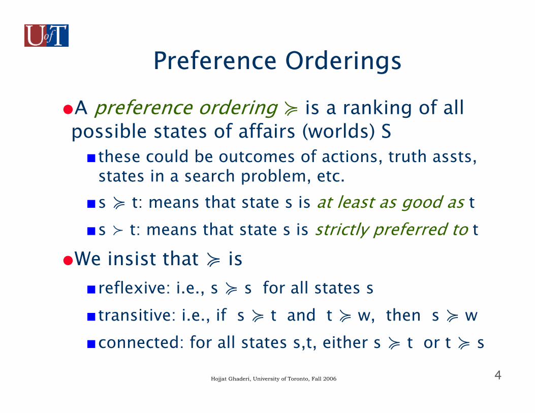
●A preference ordering ≽ is a ranking of all possible states of affairs (worlds) S■these could be outcomes of actions, truth assts,

states in a search problem, etc.■s ≽ t: means that state s is at least as good as t■s ≻ t: means that state s is strictly preferred to t

●We insist that ≽ is■reflexive: i.e., s ≽ s for all states s ■transitive: i.e., if s ≽ t and t ≽ w, then s ≽ w ■connected: for all states s,t, either s ≽ t or t ≽ s


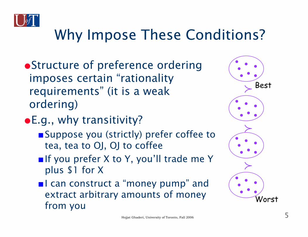
Why Impose These Conditions?

●Structure of preference ordering imposes certain “rationality requirements” (it is a weak ordering)●E.g., why transitivity?

■Suppose you (strictly) prefer coffee to tea, tea to OJ, OJ to coffee

■ If you prefer X to Y, you’ll trade me Y plus $1 for X

■ I can construct a “money pump” and extract arbitrary amounts of money from you

≻

≻

≻

Best

Worst


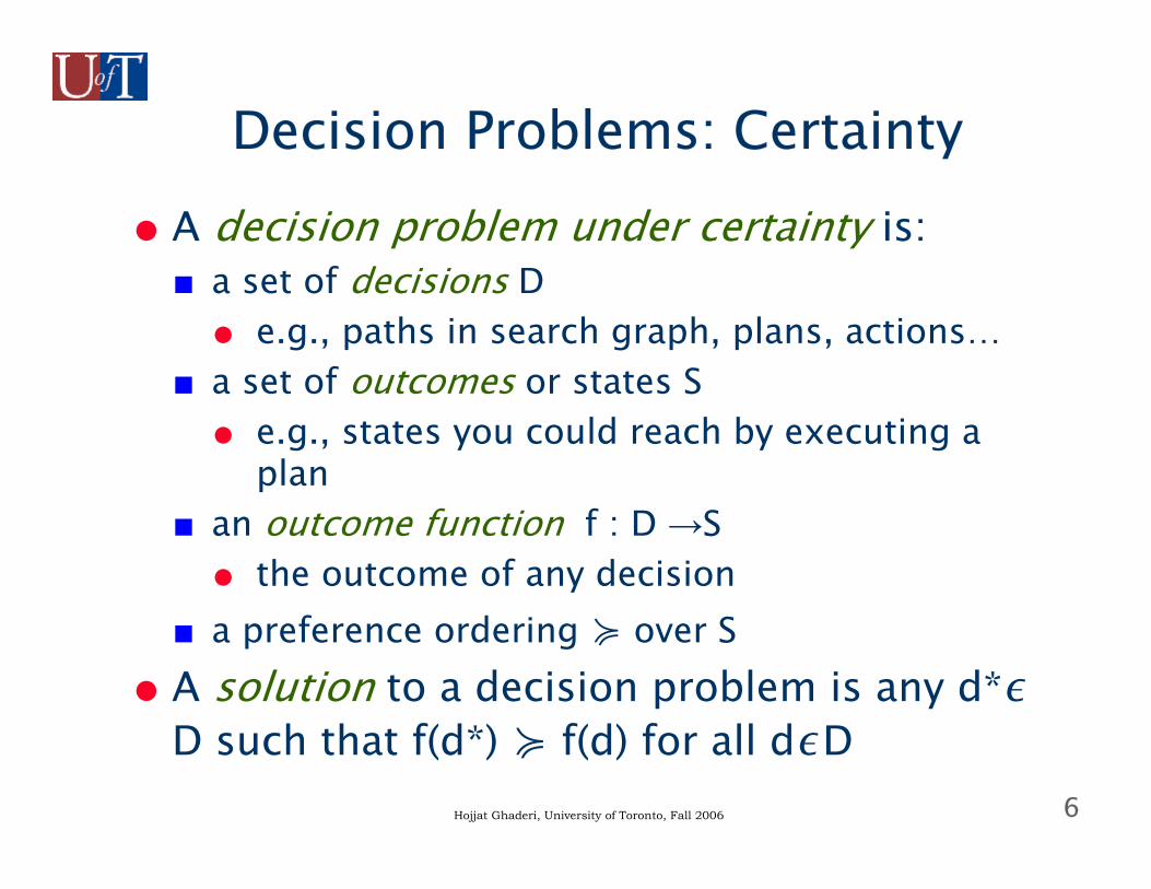
Decision Problems: Certainty● A decision problem under certainty is:■ a set of decisions D● e.g., paths in search graph, plans, actions…

■ a set of outcomes or states S● e.g., states you could reach by executing a

plan■ an outcome function f : D →S● the outcome of any decision

■ a preference ordering ≽ over S● A solution to a decision problem is any d*∊

D such that f(d*) ≽ f(d) for all d∊D


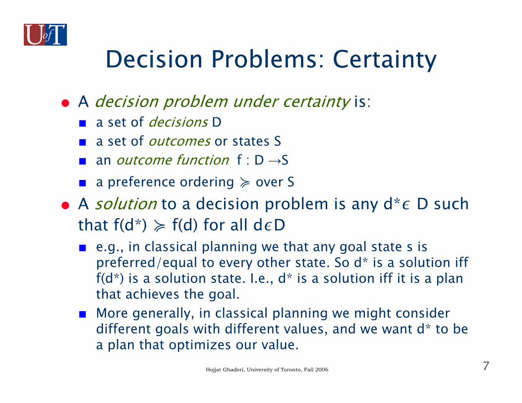
Decision Problems: Certainty● A decision problem under certainty is:

■ a set of decisions D■ a set of outcomes or states S■ an outcome function f : D →S■ a preference ordering ≽ over S

● A solution to a decision problem is any d*∊ D such that f(d*) ≽ f(d) for all d∊D■ e.g., in classical planning we that any goal state s is

preferred/equal to every other state. So d* is a solution ifff(d*) is a solution state. I.e., d* is a solution iff it is a plan that achieves the goal.

■ More generally, in classical planning we might consider different goals with different values, and we want d* to be a plan that optimizes our value.


Decision Making under Uncertainty

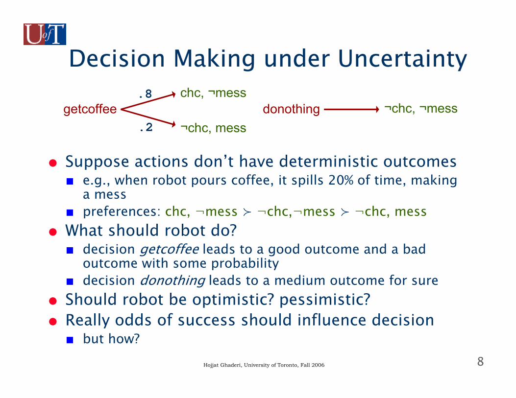
● Suppose actions don’t have deterministic outcomes■ e.g., when robot pours coffee, it spills 20% of time, making

a mess■ preferences: chc, ¬mess ≻ ¬chc,¬mess ≻ ¬chc, mess

● What should robot do?■ decision getcoffee leads to a good outcome and a bad

outcome with some probability■ decision donothing leads to a medium outcome for sure

● Should robot be optimistic? pessimistic?● Really odds of success should influence decision

■ but how?

getcoffeechc, ¬mess

¬chc, messdonothing ¬chc, ¬mess

.8

.2


Utilities

● Rather than just ranking outcomes, we must quantify our degree of preference■ e.g., how much more important is having coffee

than having tea?● A utility function U: S →ℝ associates a real-

valued utility with each outcome (state).■ U(s) quantifies our degree of preference for s

● Note: U induces a preference ordering ≽U over the states S defined as: s ≽U t iff U(s) ≥ U(t)■ ≽U is reflexive, transitive, connected


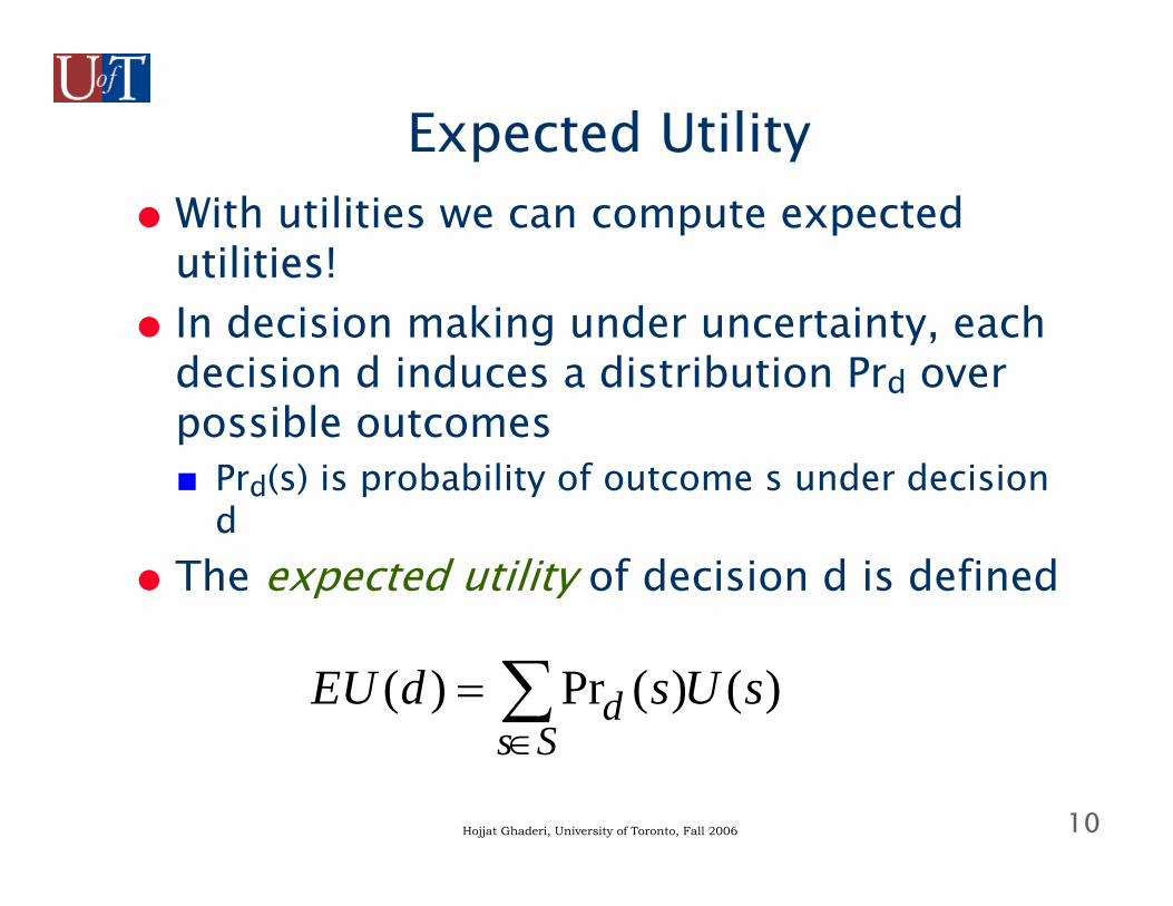
Expected Utility● With utilities we can compute expected

utilities!● In decision making under uncertainty, each

decision d induces a distribution Prd over possible outcomes■ Prd(s) is probability of outcome s under decision

d● The expected utility of decision d is defined

∑∈

=Ss

d sUsdEU )()(Pr)(


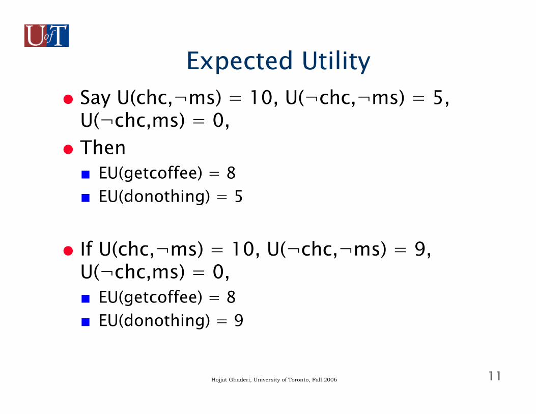
Expected Utility● Say U(chc,¬ms) = 10, U(¬chc,¬ms) = 5,

U(¬chc,ms) = 0, ● Then ■ EU(getcoffee) = 8■ EU(donothing) = 5

● If U(chc,¬ms) = 10, U(¬chc,¬ms) = 9, U(¬chc,ms) = 0,■ EU(getcoffee) = 8■ EU(donothing) = 9


The MEU Principle

● The principle of maximum expected utility (MEU) states that the optimal decision under conditions of uncertainty is the decision that has greatest expected utility.

● In our example■ if my utility function is the first one, my robot

should get coffee■ if your utility function is the second one, your robot

should do nothing


Computational Issues● At some level, solution to a dec. prob. is trivial

■ complexity lies in the fact that the decisions and outcome function are rarely specified explicitly

■ e.g., in planning or search problem, you construct the set of decisions by constructing paths or exploring search paths. Then we have to evaluate the expected utility of each. Computationally hard!

■ e.g., we find a plan achieving some expected utility e● Can we stop searching?● Must convince ourselves no better plan exists● Generally requires searching entire plan space, unless

we have some clever tricks


Decision Problems: Uncertainty●A decision problem under uncertainty is:

■a set of decisions D■a set of outcomes or states S■an outcome function Pr : D →∆(S)

●∆(S) is the set of distributions over S (e.g., Prd)

■a utility function U over S●A solution to a decision problem under uncertainty is any d*∊ D such that EU(d*) ≽EU(d) for all d∊D


Expected Utility: Notes

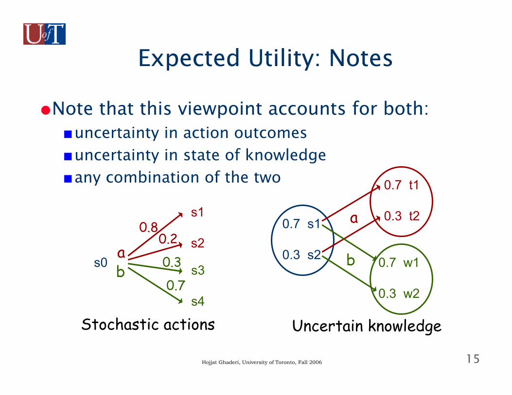
●Note that this viewpoint accounts for both:■uncertainty in action outcomes■uncertainty in state of knowledge■any combination of the two

s0

s1

s2a0.8

0.2

s3

s4

b 0.3

0.7

0.7 s1

0.3 s2

0.7 t1

0.3 t2

0.7 w1

0.3 w2

a

b

Stochastic actions Uncertain knowledge


Expected Utility: Notes

●Why MEU? Where do utilities come from?■underlying foundations of utility theory tightly

couple utility with action/choice■a utility function can be determined by asking

someone about their preferences for actions in specific scenarios (or “lotteries” over outcomes)

●Utility functions needn’t be unique■ if I multiply U by a positive constant, all decisions

have same relative utility■ if I add a constant to U, same thing■U is unique up to positive affine transformation


So What are the Complications?●Outcome space is large

■ like all of our problems, states spaces can be huge

■don’t want to spell out distributions like Prdexplicitly

■Soln: Bayes nets (or related: influence diagrams)


So What are the Complications?●Decision space is large

■usually our decisions are not one-shot actions■rather they involve sequential choices (like plans)■ if we treat each plan as a distinct decision,

decision space is too large to handle directly■Soln: use dynamic programming methods to

construct optimal plans (actually generalizations of plans, called policies… like in game trees)


An Simple Example● Suppose we have two actions: a, b● We have time to execute two actions in

sequence● This means we can do either:■ [a,a], [a,b], [b,a], [b,b]

● Actions are stochastic: action a induces distribution Pra(si | sj) over states■ e.g., Pra(s2 | s1) = .9 means prob. of moving to

state s2 when a is performed at s1 is .9■ similar distribution for action b

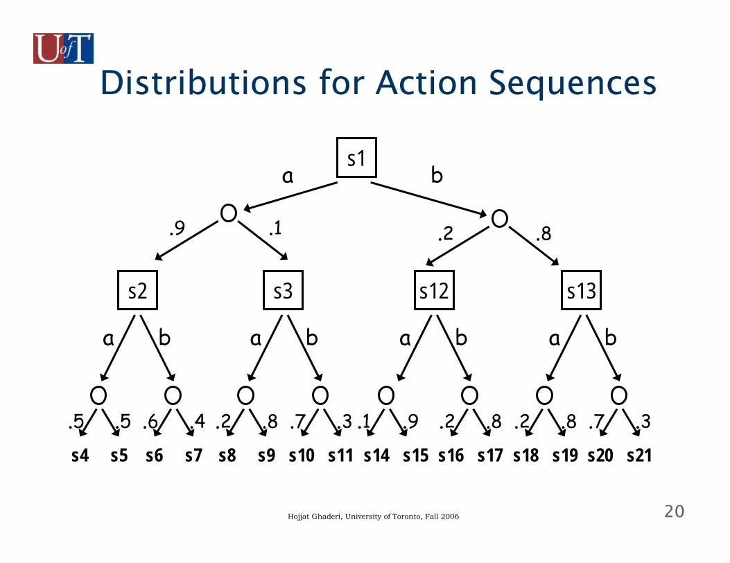
● How good is a particular sequence of actions?


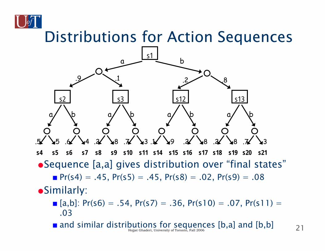
Distributions for Action Sequences

s1

s13s12s3s2

a b

.9 .1 .2 .8

s4 s5

.5 .5s6 s7

.6 .4

a b

s8 s9

.2 .8s10 s11

.7 .3

a b

s14 s15

.1 .9s16 s17

.2 .8

a b

s18 s19

.2 .8s20 s21

.7 .3

a b


Distributions for Action Sequences

●Sequence [a,a] gives distribution over “final states”■ Pr(s4) = .45, Pr(s5) = .45, Pr(s8) = .02, Pr(s9) = .08

●Similarly:■ [a,b]: Pr(s6) = .54, Pr(s7) = .36, Pr(s10) = .07, Pr(s11) =

.03■ and similar distributions for sequences [b,a] and [b,b]

s1

s13s12s3s2

a b

.9 .1 .2 .8

s4 s5.5 .5

s6 s7.6 .4

a b

s8 s9.2 .8

s10 s11.7 .3

a b

s14 s15.1 .9

s16 s17.2 .8

a b

s18 s19.2 .8

s20 s21.7 .3

a b


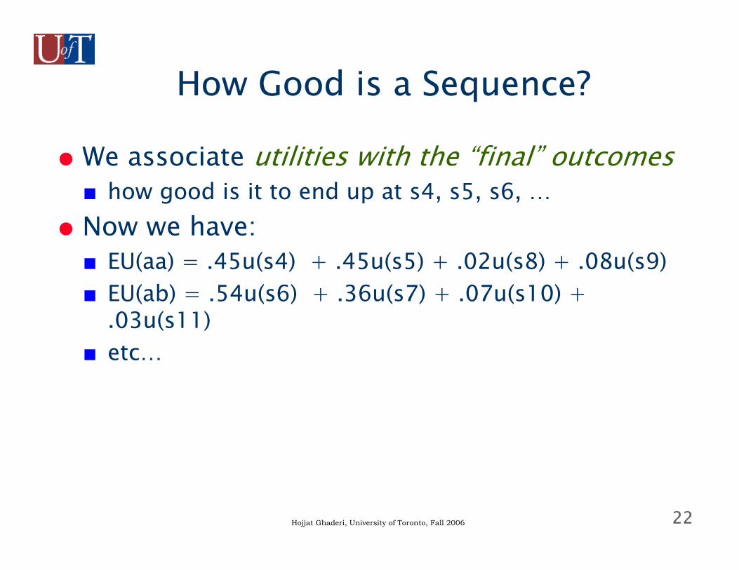
How Good is a Sequence?

● We associate utilities with the “final” outcomes■ how good is it to end up at s4, s5, s6, …

● Now we have:■ EU(aa) = .45u(s4) + .45u(s5) + .02u(s8) + .08u(s9)■ EU(ab) = .54u(s6) + .36u(s7) + .07u(s10) +

.03u(s11)■ etc…


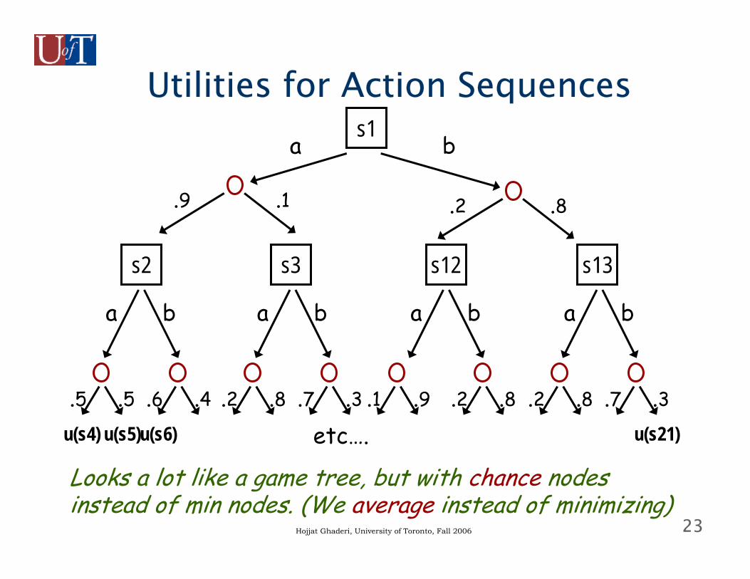
Utilities for Action Sequencess1

s13s12s3s2

a b

.9 .1 .2 .8

u(s4) u(s5)

.5 .5u(s6)

.6 .4

a b

.2 .8 .7 .3

a b

.1 .9 .2 .8

a b

.2 .8u(s21)

.7 .3

a b

etc….

Looks a lot like a game tree, but with chance nodesinstead of min nodes. (We average instead of minimizing)


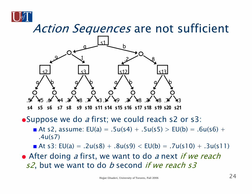
Action Sequences are not sufficient

●Suppose we do a first; we could reach s2 or s3:■ At s2, assume: EU(a) = .5u(s4) + .5u(s5) > EU(b) = .6u(s6) +

.4u(s7)■ At s3: EU(a) = .2u(s8) + .8u(s9) < EU(b) = .7u(s10) + .3u(s11)

● After doing a first, we want to do a next if we reach s2, but we want to do b second if we reach s3

s1

s13s12s3s2

a b

.9 .1 .2 .8

s4 s5.5 .5

s6 s7.6 .4

a b

s8 s9.2 .8

s10 s11.7 .3

a b

s14 s15.1 .9

s16 s17.2 .8

a b

s18 s19.2 .8

s20 s21.7 .3

a b


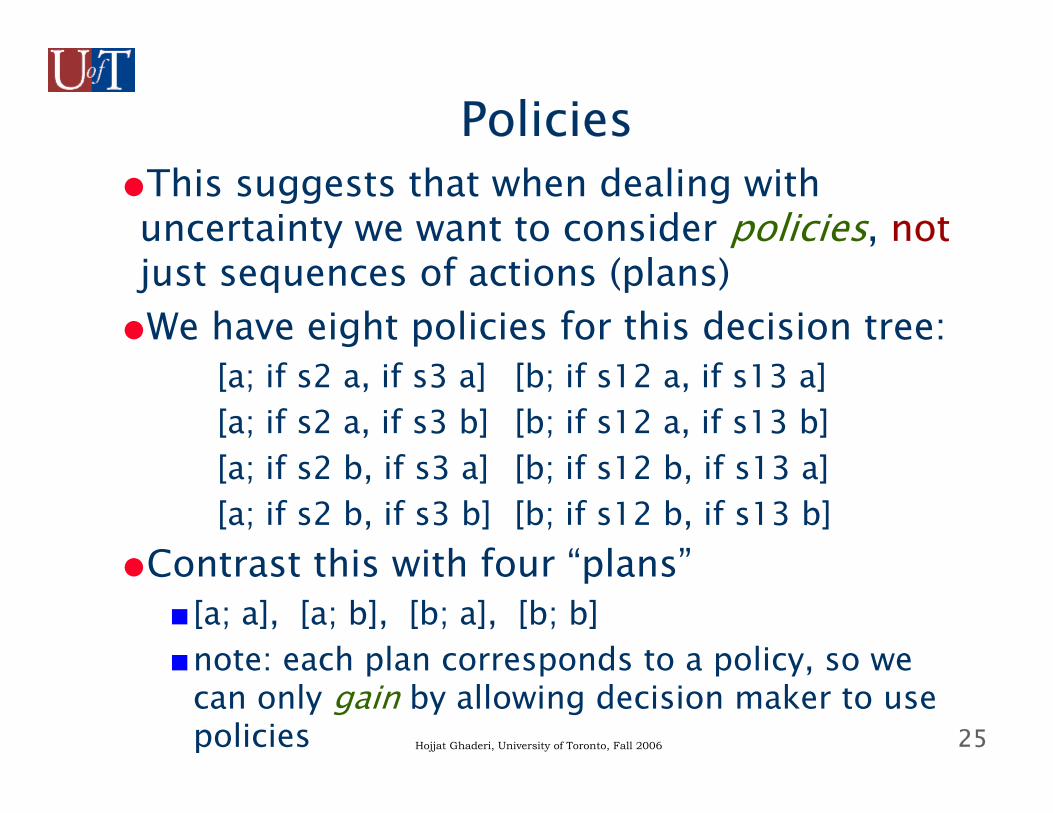
Policies●This suggests that when dealing with uncertainty we want to consider policies, notjust sequences of actions (plans)●We have eight policies for this decision tree:

[a; if s2 a, if s3 a] [b; if s12 a, if s13 a][a; if s2 a, if s3 b] [b; if s12 a, if s13 b][a; if s2 b, if s3 a] [b; if s12 b, if s13 a][a; if s2 b, if s3 b] [b; if s12 b, if s13 b]

●Contrast this with four “plans”■[a; a], [a; b], [b; a], [b; b]■note: each plan corresponds to a policy, so we

can only gain by allowing decision maker to use policies


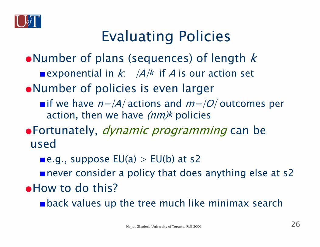
Evaluating Policies●Number of plans (sequences) of length k

■exponential in k: |A|k if A is our action set●Number of policies is even larger

■ if we have n=|A| actions and m=|O| outcomes per action, then we have (nm)k policies

●Fortunately, dynamic programming can be used■e.g., suppose EU(a) > EU(b) at s2■never consider a policy that does anything else at s2

●How to do this?■back values up the tree much like minimax search


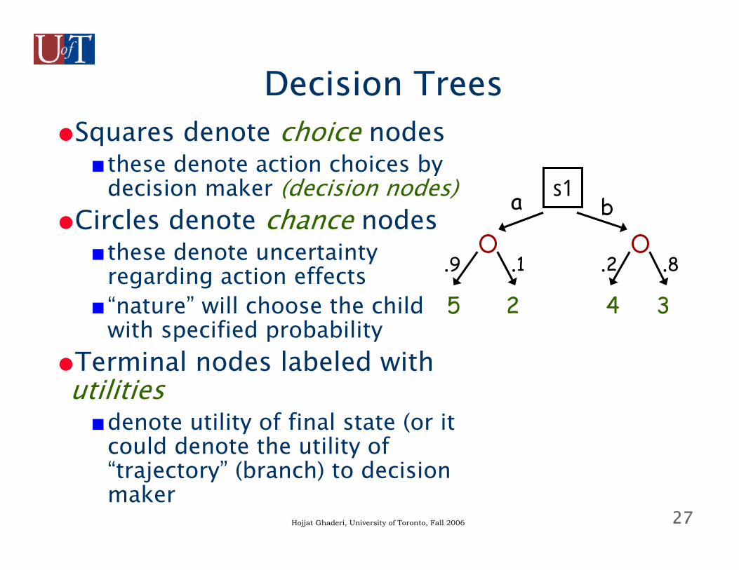
Decision Trees●Squares denote choice nodes

■these denote action choices by decision maker (decision nodes)

●Circles denote chance nodes■these denote uncertainty

regarding action effects■“nature” will choose the child

with specified probability●Terminal nodes labeled with utilities■denote utility of final state (or it

could denote the utility of “trajectory” (branch) to decision maker

s1a b

.9 .1 .2 .8

5 2 4 3


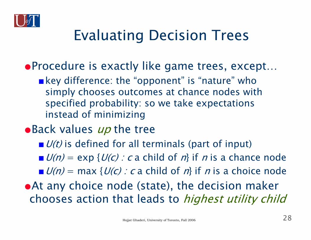
Evaluating Decision Trees

●Procedure is exactly like game trees, except…■key difference: the “opponent” is “nature” who

simply chooses outcomes at chance nodes with specified probability: so we take expectations instead of minimizing

●Back values up the tree■U(t) is defined for all terminals (part of input)■U(n) = exp {U(c) : c a child of n} if n is a chance node■U(n) = max {U(c) : c a child of n} if n is a choice node

●At any choice node (state), the decision maker chooses action that leads to highest utility child


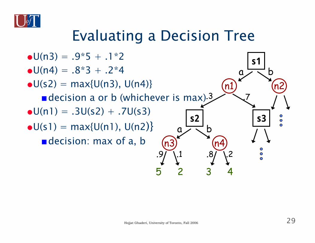
Evaluating a Decision Tree●U(n3) = .9*5 + .1*2●U(n4) = .8*3 + .2*4●U(s2) = max{U(n3), U(n4)}

■decision a or b (whichever is max)●U(n1) = .3U(s2) + .7U(s3)●U(s1) = max{U(n1), U(n2)}

■decision: max of a, b

s2

n3a b

.9 .1

5 2

n4.8 .2

3 4

s1

n1a b

.3 .7n2

s3


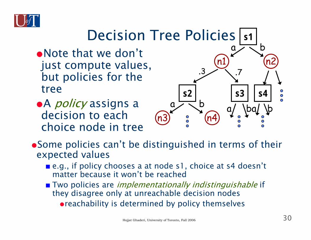
Decision Tree Policies●Note that we don’t just compute values, but policies for the tree●A policy assigns a decision to each choice node in tree

●Some policies can’t be distinguished in terms of their expected values■ e.g., if policy chooses a at node s1, choice at s4 doesn’t

matter because it won’t be reached■ Two policies are implementationally indistinguishable if

they disagree only at unreachable decision nodes●reachability is determined by policy themselves

s2

n3a b

n4

s1

n1a b

.3 .7n2

s3 s4a bab


Key Assumption: Observability●Full observability: we must know the initial state and outcome of each action■specifically, to implement the policy, we must be

able to resolve the uncertainty of any chance node that is followed by a decision node

■e.g., after doing a at s1, we must know which of the outcomes (s2 or s3) was realized so we know what action to do next (note: s2 and s3 may prescribe different ations)


Computational Issues

●Savings compared to explicit policy evaluation is substantial●Evaluate only O((nm)d ) nodes in tree of depth d

■total computational cost is thus O((nm)d ) ●Note that this is how many policies there are

■but evaluating a single policy explicitly requires substantial computation: O(nmd )

■total computation for explicity evaluating each policy would be O(ndm2d ) !!!

●Tremendous value to dynamic programming solution


Computational Issues

●Tree size: grows exponentially with depth●Possible solutions:

■bounded lookahead with heuristics (like game trees)■heuristic search procedures (like A*)


Other Issues

●Specification: suppose each state is an assignment to variables; then representing action probability distributions is complex (and branching factor could be immense)●Possible solutions:

■represent distribution using Bayes nets■solve problems using decision networks (or

influence diagrams)


Large State Spaces (Variables)

●To represent outcomes of actions or decisions, we need to specify distributions ■Pr(s|d) : probability of outcome s given decision d■Pr(s|a,s’): prob. of state s given that action a

performed in state s’●But state space exponential in # of variables

■spelling out distributions explicitly is intractable●Bayes nets can be used to represent actions

■this is just a joint distribution over variables, conditioned on action/decision and previous state


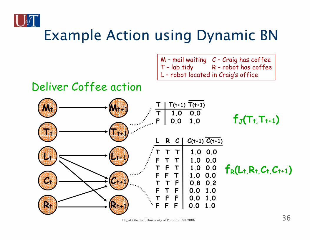
Example Action using Dynamic BN

Tt

Lt

Ct

Rt

Tt+1

Lt+1

Ct+1

Rt+1

Deliver Coffee action

fR(Lt,Rt,Ct,Ct+1)

fJ(Tt,Tt+1)

L R C C(t+1) C(t+1)

T T T 1.0 0.0F T T 1.0 0.0T F T 1.0 0.0F F T 1.0 0.0T T F 0.8 0.2F T F 0.0 1.0T F F 0.0 1.0F F F 0.0 1.0

T T(t+1) T(t+1)T 1.0 0.0F 0.0 1.0

Mt Mt+1

M – mail waiting C – Craig has coffeeT – lab tidy R – robot has coffeeL – robot located in Craig’s office


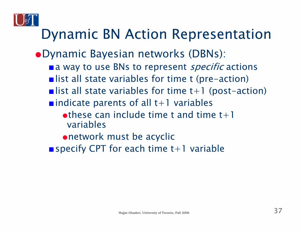
Dynamic BN Action Representation●Dynamic Bayesian networks (DBNs):

■a way to use BNs to represent specific actions■ list all state variables for time t (pre-action)■ list all state variables for time t+1 (post-action)■ indicate parents of all t+1 variables

●these can include time t and time t+1 variables●network must be acyclic

■specify CPT for each time t+1 variable


Dynamic BN Action Representation●Note: generally no prior given for time t variables■we’re (generally) interested in conditional

distribution over post-action states given pre-action state

■so time t vars are instantiated as “evidence” when using a DBN (generally)


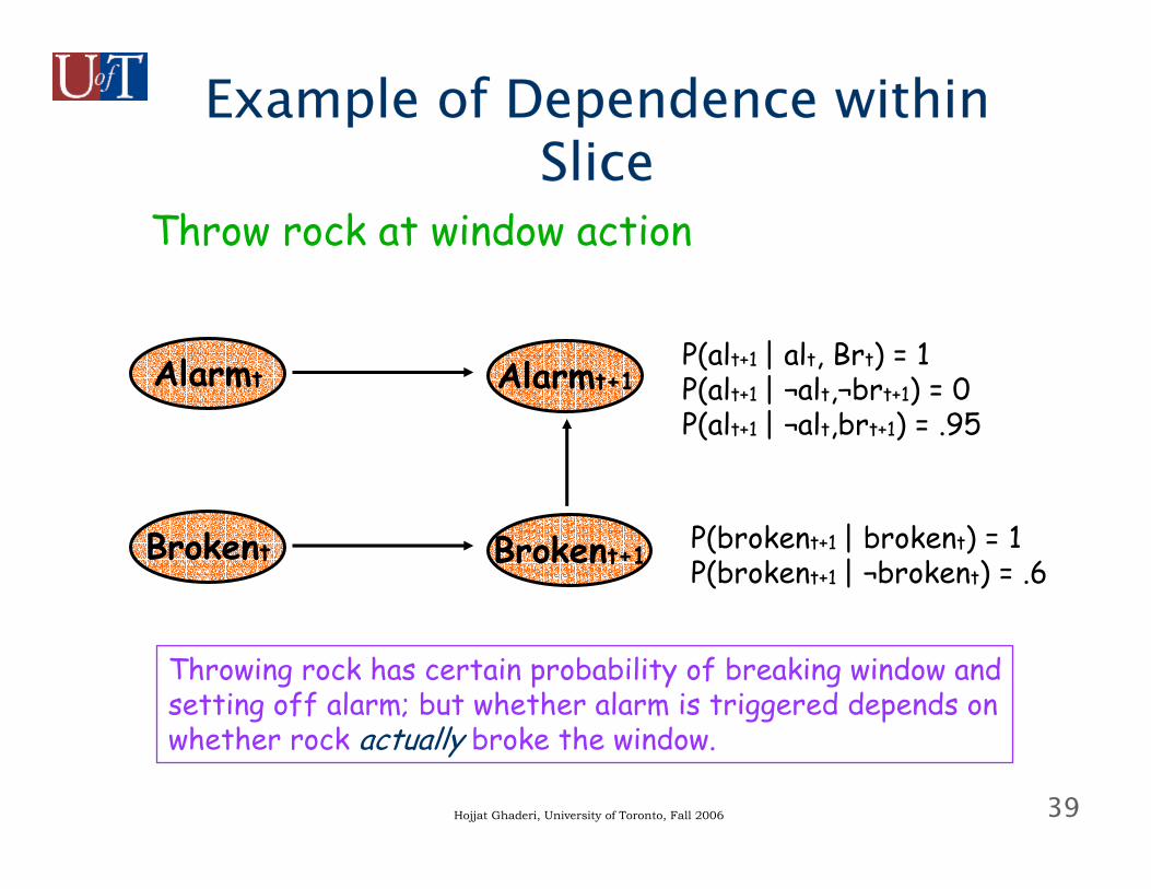
Example of Dependence within Slice

Throw rock at window action

Alarmt Alarmt+1

Brokent Brokent+1 P(brokent+1 | brokent) = 1P(brokent+1 | ¬brokent) = .6

P(alt+1 | alt, Brt) = 1P(alt+1 | ¬alt,¬brt+1) = 0P(alt+1 | ¬alt,brt+1) = .95

Throwing rock has certain probability of breaking window andsetting off alarm; but whether alarm is triggered depends onwhether rock actually broke the window.


Use of BN Action Reprsnt’n●DBNs: actions concisely,naturally specified

■These look a bit like STRIPS and the situtationcalculus, but allow for probabilistic effects


Use of BN Action Reprsnt’n●How to use:

■use to generate “expectimax” search tree to solve decision problems

■use directly in stochastic decision making algorithms

●First use doesn’t buy us much computationally when solving decision problems. But second use allows us to compute expected utilities without enumerating the outcome space (tree)■well see something like this with decision

networks


Decision Networks●Decision networks (more commonly known as influence diagrams) provide a way of representing sequential decision problems■basic idea: represent the variables in the problem

as you would in a BN■add decision variables – variables that you

“control”■add utility variables – how good different states

are


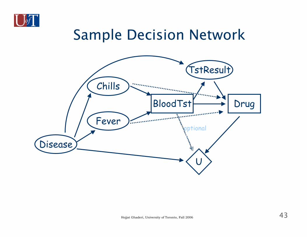
Sample Decision Network

Disease

TstResultChills

Fever

BloodTst Drug

U

optional


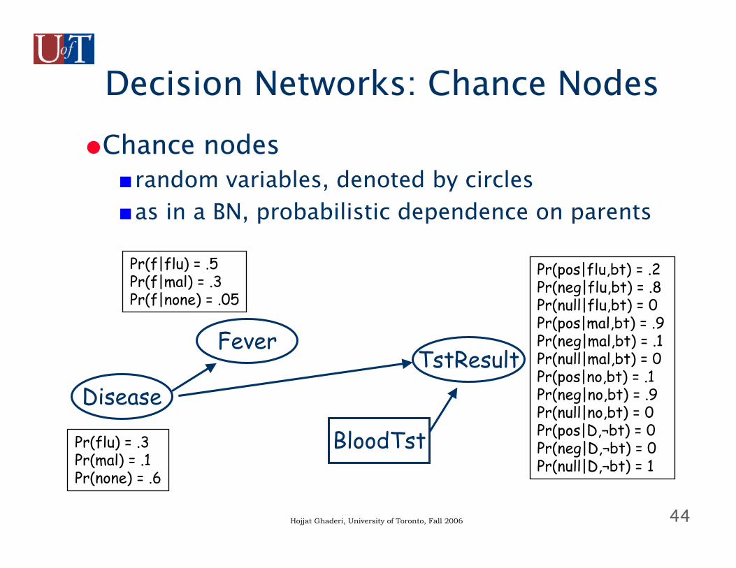
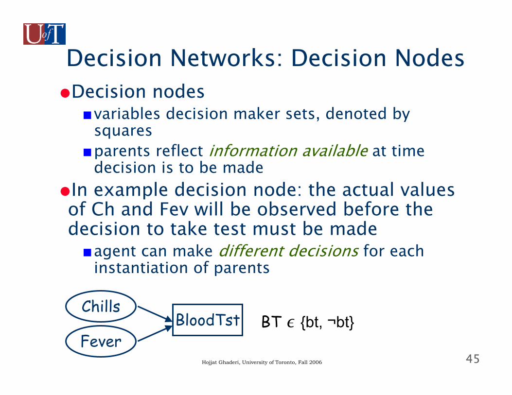
Decision Networks: Decision Nodes●Decision nodes

■variables decision maker sets, denoted by squares

■parents reflect information available at time decision is to be made

●In example decision node: the actual values of Ch and Fev will be observed before the decision to take test must be made■agent can make different decisions for each

instantiation of parents

Chills

FeverBloodTst BT ∊ {bt, ¬bt}


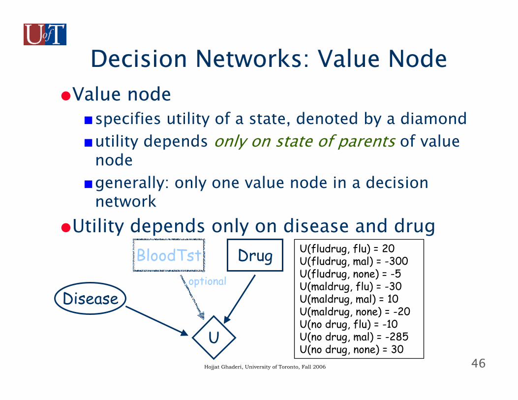
Decision Networks: Value Node●Value node

■specifies utility of a state, denoted by a diamond■utility depends only on state of parents of value

node■generally: only one value node in a decision

network●Utility depends only on disease and drug

Disease

BloodTst Drug

U

optional

U(fludrug, flu) = 20U(fludrug, mal) = -300U(fludrug, none) = -5U(maldrug, flu) = -30U(maldrug, mal) = 10U(maldrug, none) = -20U(no drug, flu) = -10U(no drug, mal) = -285U(no drug, none) = 30


Decision Networks: Assumptions●Decision nodes are totally ordered

■decision variables D1, D2, …, Dn■decisions are made in sequence■e.g., BloodTst (yes,no) decided before Drug

(fd,md,no)


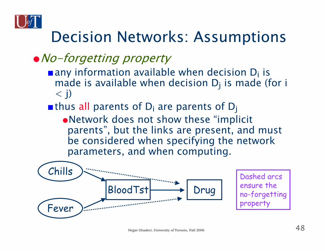
Decision Networks: Assumptions●No-forgetting property

■any information available when decision Di is made is available when decision Dj is made (for i < j)

■thus all parents of Di are parents of Dj●Network does not show these “implicit parents”, but the links are present, and must be considered when specifying the network parameters, and when computing.

Chills

Fever

BloodTst DrugDashed arcsensure theno-forgettingproperty


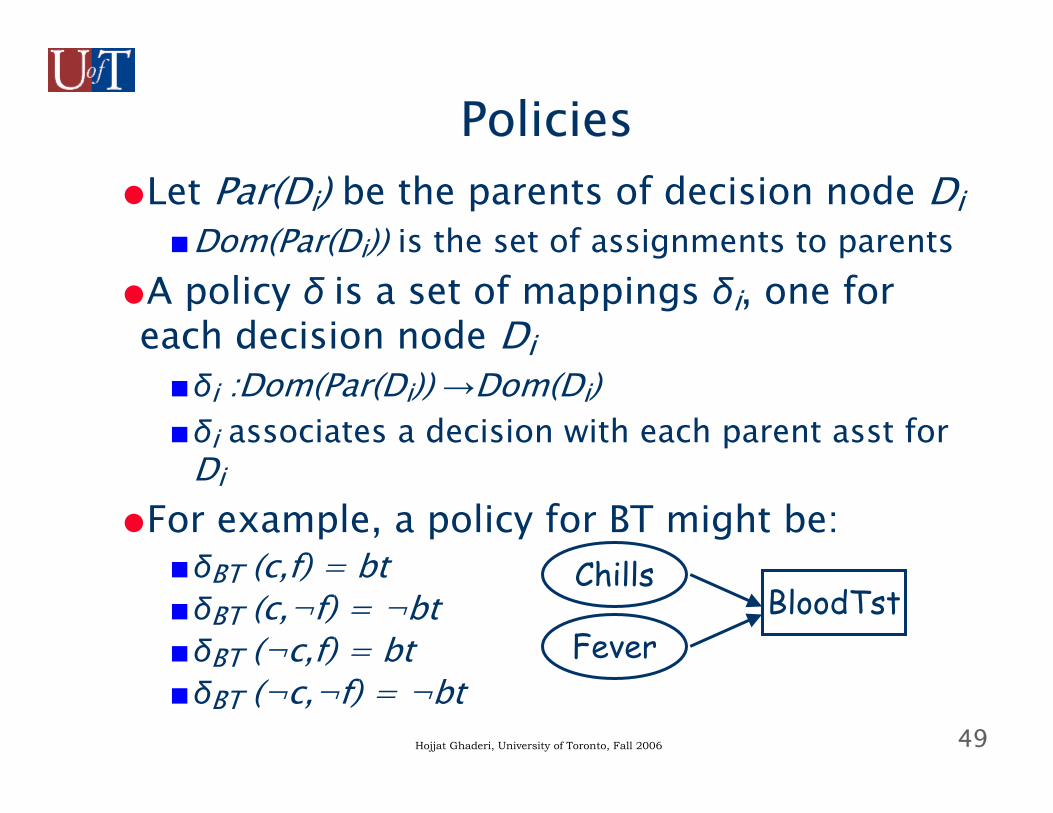
Policies●Let Par(Di) be the parents of decision node Di

■Dom(Par(Di)) is the set of assignments to parents●A policy δ is a set of mappings δi, one for each decision node Di■δi :Dom(Par(Di)) →Dom(Di)■δi associates a decision with each parent asst for

Di●For example, a policy for BT might be:

■δBT (c,f) = bt■δBT (c,¬f) = ¬bt■δBT (¬c,f) = bt■δBT (¬c,¬f) = ¬bt

Chills

FeverBloodTst


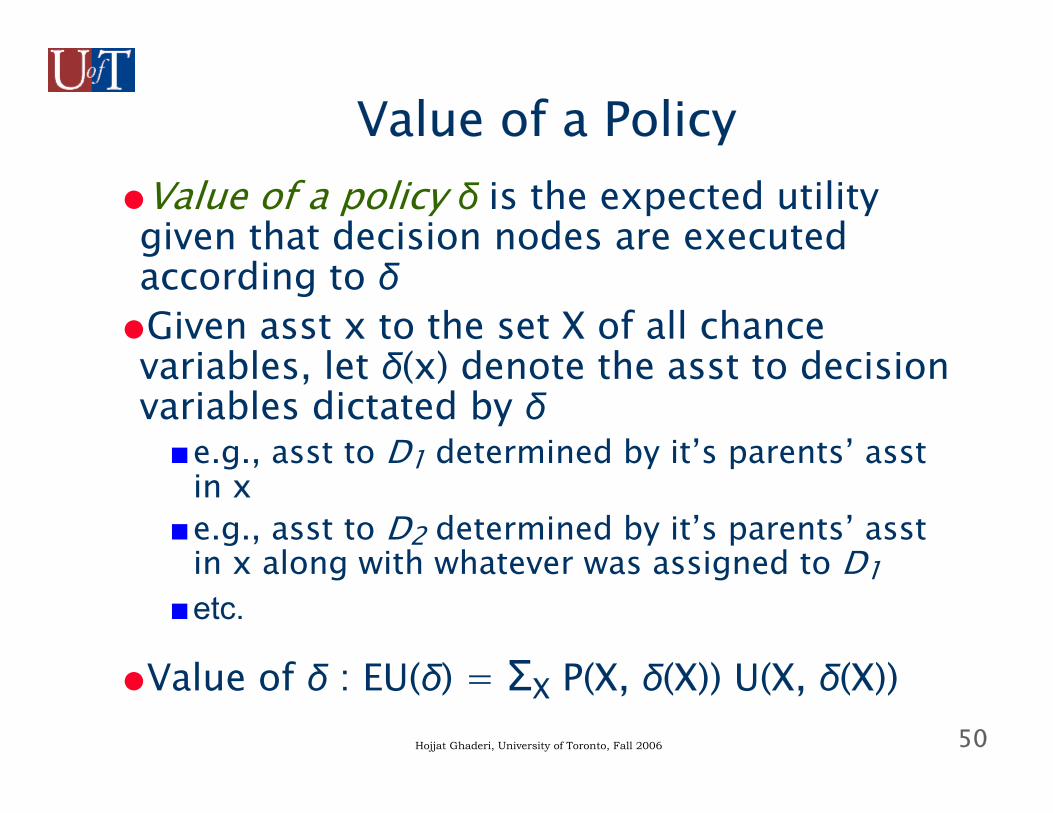
Value of a Policy●Value of a policy δ is the expected utility given that decision nodes are executed according to δ●Given asst x to the set X of all chance variables, let δ(x) denote the asst to decision variables dictated by δ■e.g., asst to D1 determined by it’s parents’ asst

in x■e.g., asst to D2 determined by it’s parents’ asst

in x along with whatever was assigned to D1■etc.

●Value of δ : EU(δ) = ΣX P(X, δ(X)) U(X, δ(X))


Optimal Policies

●An optimal policy is a policy δ* such that EU(δ*) ≥ EU(δ) for all policies δ

●We can use the dynamic programming principle to avoid enumerating all policies●We can also use the structure of the decision network to use variable elimination to aid in the computation


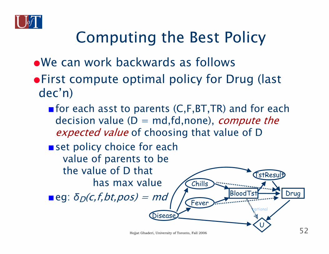
Computing the Best Policy●We can work backwards as follows●First compute optimal policy for Drug (last dec’n)■for each asst to parents (C,F,BT,TR) and for each

decision value (D = md,fd,none), compute the expected value of choosing that value of D

■set policy choice for eachvalue of parents to bethe value of D that

has max value■eg: δD(c,f,bt,pos) = md

Disease

TstResultChills

FeverBloodTst Drug

U

optional


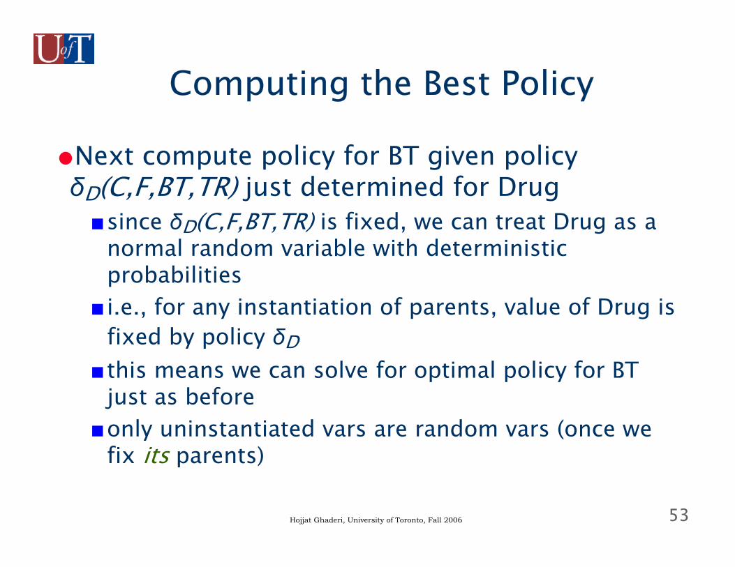
Computing the Best Policy

●Next compute policy for BT given policy δD(C,F,BT,TR) just determined for Drug■since δD(C,F,BT,TR) is fixed, we can treat Drug as a

normal random variable with deterministic probabilities

■ i.e., for any instantiation of parents, value of Drug is fixed by policy δD

■this means we can solve for optimal policy for BT just as before

■only uninstantiated vars are random vars (once we fix its parents)


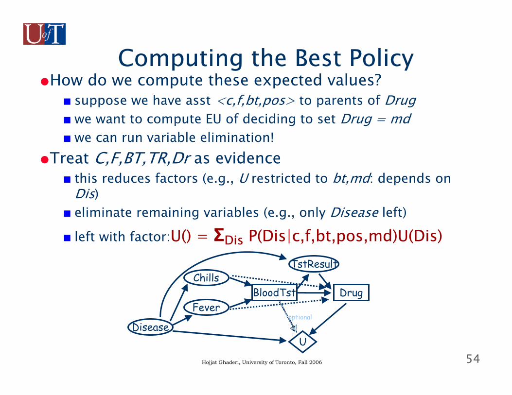
Computing the Best Policy●How do we compute these expected values?

■ suppose we have asst <c,f,bt,pos> to parents of Drug■we want to compute EU of deciding to set Drug = md■we can run variable elimination!

●Treat C,F,BT,TR,Dr as evidence■ this reduces factors (e.g., U restricted to bt,md: depends on

Dis)■ eliminate remaining variables (e.g., only Disease left)

■ left with factor:U() = ΣDis P(Dis|c,f,bt,pos,md)U(Dis)

Disease

TstResultChills

FeverBloodTst Drug

U

optional


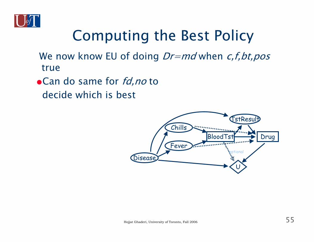
Computing the Best PolicyWe now know EU of doing Dr=md when c,f,bt,postrue●Can do same for fd,no to

decide which is best

Disease

TstResultChills

FeverBloodTst Drug

U

optional


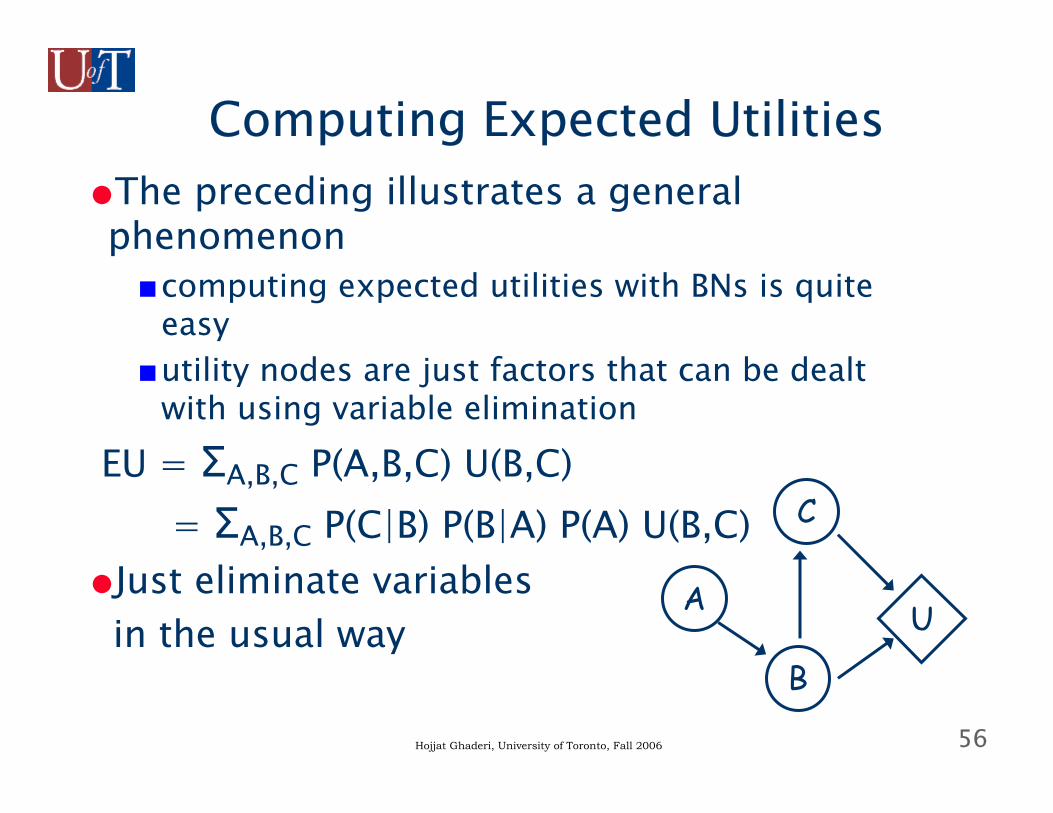
Computing Expected Utilities●The preceding illustrates a general phenomenon■computing expected utilities with BNs is quite

easy■utility nodes are just factors that can be dealt

with using variable elimination

EU = ΣA,B,C P(A,B,C) U(B,C)= ΣA,B,C P(C|B) P(B|A) P(A) U(B,C)

●Just eliminate variablesin the usual way U

C

B

A


Optimizing Policies: Key Points●If a decision node D has no decisions that follow it, we can find its policy by instantiating each of its parents and computing the expected utility of each decision for each parent instantiation


Optimizing Policies: Key Points

■no-forgetting means that all other decisions are instantiated (they must be parents)

■ its easy to compute the expected utility using VE■the number of computations is quite large: we

run expected utility calculations (VE) for each parent instantiation together with each possible decision D might allow

■policy: choose max decision for each parent instant’n


Optimizing Policies: Key Points

●When a decision D node is optimized, it can be treated as a random variable■for each instantiation of its parents we now know

what value the decision should take■just treat policy as a new CPT: for a given parent

instantiation x, D gets δ(x) with probability 1(all other decisions get probability zero)

●If we optimize from last decision to first, at each point we can optimize a specific decision by (a bunch of) simple VE calculations■ it’s successor decisions (optimized) are just normal

nodes in the BNs (with CPTs)


Decision Network Notes

●Decision networks commonly used by decision analysts to help structure decision problems●Much work put into computationally effective techniques to solve these●Complexity much greater than BN inference

■we need to solve a number of BN inference problems

■one BN problem for each setting of decision node parents and decision node value


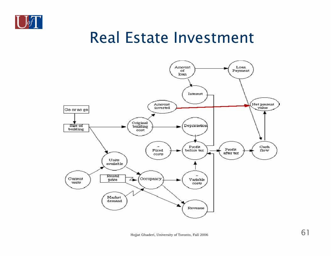
Real Estate Investment


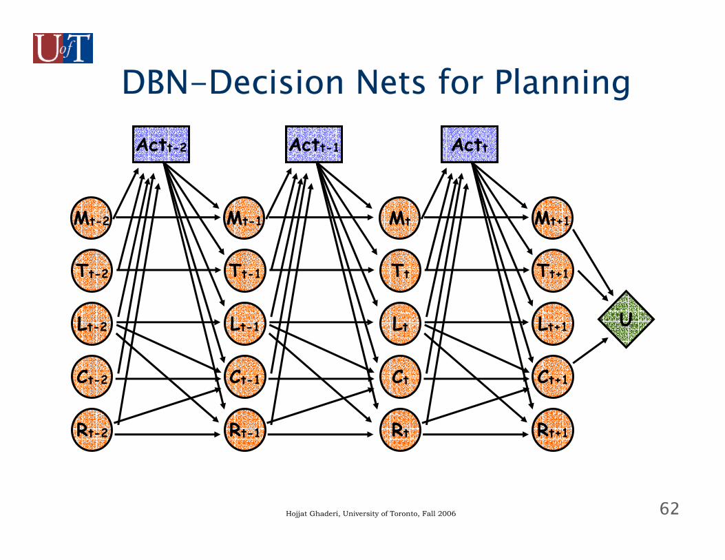
DBN-Decision Nets for Planning

Tt

Lt

Ct

Rt

Tt+1

Lt+1

Ct+1

Rt+1

Mt Mt+1

Actt

U

Tt-1

Lt-1

Ct-1

Rt-1

Mt-1

Actt-1

Tt-2

Lt-2

Ct-2

Rt-2

Mt-2

Actt-2


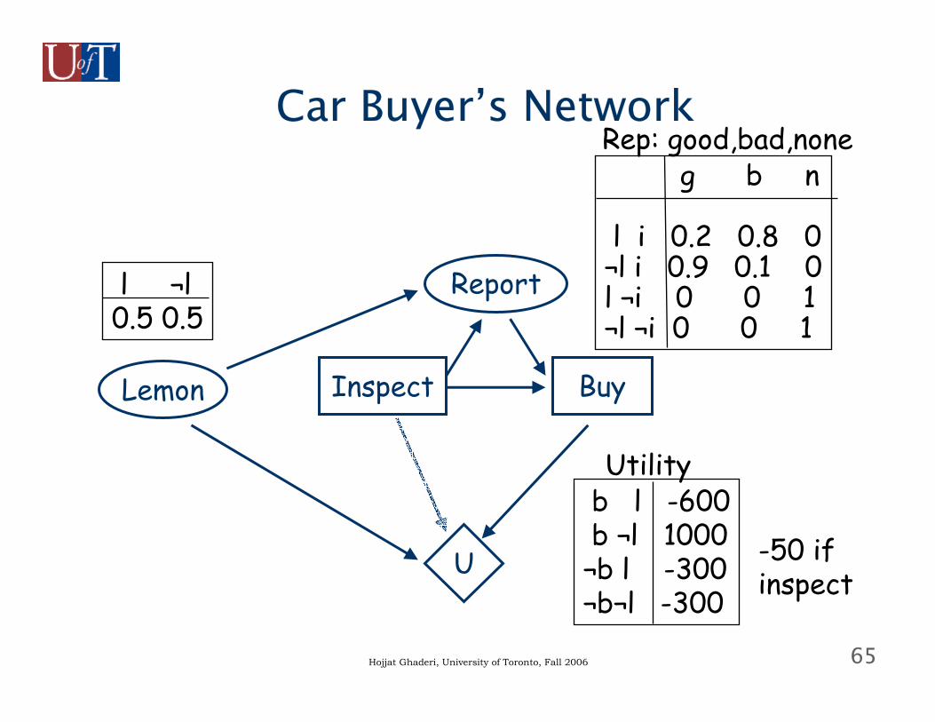
A Detailed Decision Net Example● Setting: you want to buy a used car, but

there’s a good chance it is a “lemon” (i.e., prone to breakdown). Before deciding to buy it, you can take it to a mechanic for inspection. They will give you a report on the car, labeling it either “good” or “bad”. A good report is positively correlated with the car being sound, while a bad report is positively correlated with the car being a lemon.


A Detailed Decision Net Example● However the report costs $50. So you could

risk it, and buy the car without the report.● Owning a sound car is better than having

no car, which is better than owning a lemon.


Car Buyer’s Network

Lemon

Report

Inspect Buy

U

l ¬l0.5 0.5

g b n

l i 0.2 0.8 0¬l i 0.9 0.1 0l ¬i 0 0 1¬l ¬i 0 0 1

Rep: good,bad,none

b l -600b ¬l 1000

¬b l -300¬b¬l -300

Utility

-50 ifinspect


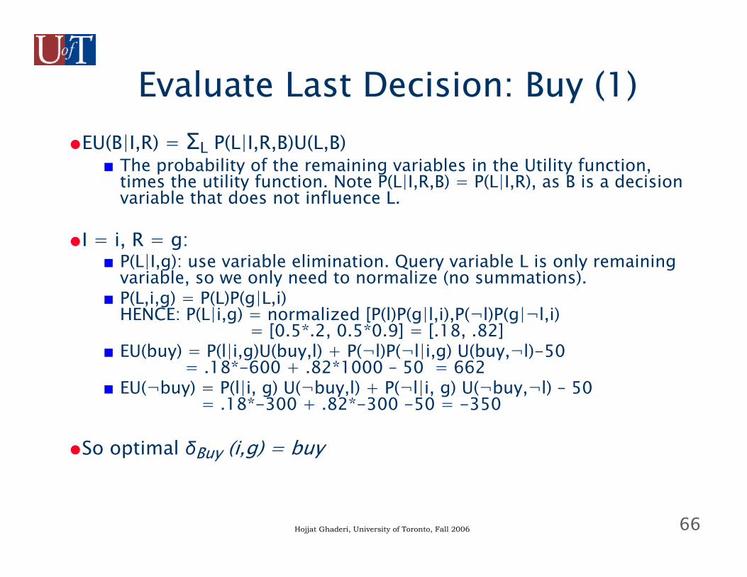
Evaluate Last Decision: Buy (1)●EU(B|I,R) = ΣL P(L|I,R,B)U(L,B)

■ The probability of the remaining variables in the Utility function, times the utility function. Note P(L|I,R,B) = P(L|I,R), as B is a decision variable that does not influence L.

●I = i, R = g:■ P(L|I,g): use variable elimination. Query variable L is only remaining

variable, so we only need to normalize (no summations).■ P(L,i,g) = P(L)P(g|L,i)

HENCE: P(L|i,g) = normalized [P(l)P(g|l,i),P(¬l)P(g|¬l,i)= [0.5*.2, 0.5*0.9] = [.18, .82]

■ EU(buy) = P(l|i,g)U(buy,l) + P(¬l)P(¬l|i,g) U(buy,¬l)-50= .18*-600 + .82*1000 – 50 = 662

■ EU(¬buy) = P(l|i, g) U(¬buy,l) + P(¬l|i, g) U(¬buy,¬l) – 50= .18*-300 + .82*-300 -50 = -350

●So optimal δBuy (i,g) = buy


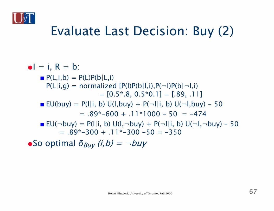
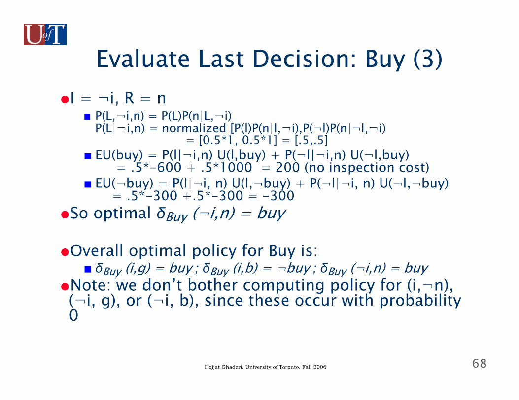
Evaluate Last Decision: Buy (3)●I = ¬i, R = n

■ P(L,¬i,n) = P(L)P(n|L,¬i)P(L|¬i,n) = normalized [P(l)P(n|l,¬i),P(¬l)P(n|¬l,¬i)

= [0.5*1, 0.5*1] = [.5,.5]■ EU(buy) = P(l|¬i,n) U(l,buy) + P(¬l|¬i,n) U(¬l,buy)

= .5*-600 + .5*1000 = 200 (no inspection cost)■ EU(¬buy) = P(l|¬i, n) U(l,¬buy) + P(¬l|¬i, n) U(¬l,¬buy)

= .5*-300 +.5*-300 = -300●So optimal δBuy (¬i,n) = buy

●Overall optimal policy for Buy is:■ δBuy (i,g) = buy ; δBuy (i,b) = ¬buy ; δBuy (¬i,n) = buy

●Note: we don’t bother computing policy for (i,¬n), (¬i, g), or (¬i, b), since these occur with probability 0


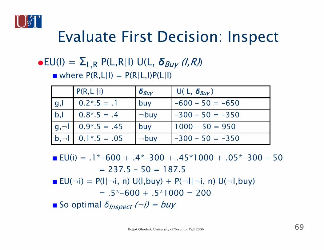
Evaluate First Decision: Inspect●EU(I) = ΣL,R P(L,R|I) U(L, δBuy (I,R))

■where P(R,L|I) = P(R|L,I)P(L|I)

■ EU(i) = .1*-600 + .4*-300 + .45*1000 + .05*-300 - 50= 237.5 – 50 = 187.5

■ EU(¬i) = P(l|¬i, n) U(l,buy) + P(¬l|¬i, n) U(¬l,buy)= .5*-600 + .5*1000 = 200

■ So optimal δInspect (¬i) = buy

-300 - 50 = -350¬buy0.1*.5 = .05b,¬l1000 - 50 = 950buy0.9*.5 = .45g,¬l-300 - 50 = -350¬buy0.8*.5 = .4b,l-600 - 50 = -650buy0.2*.5 = .1g,lU( L, δBuy )δBuyP(R,L |i)


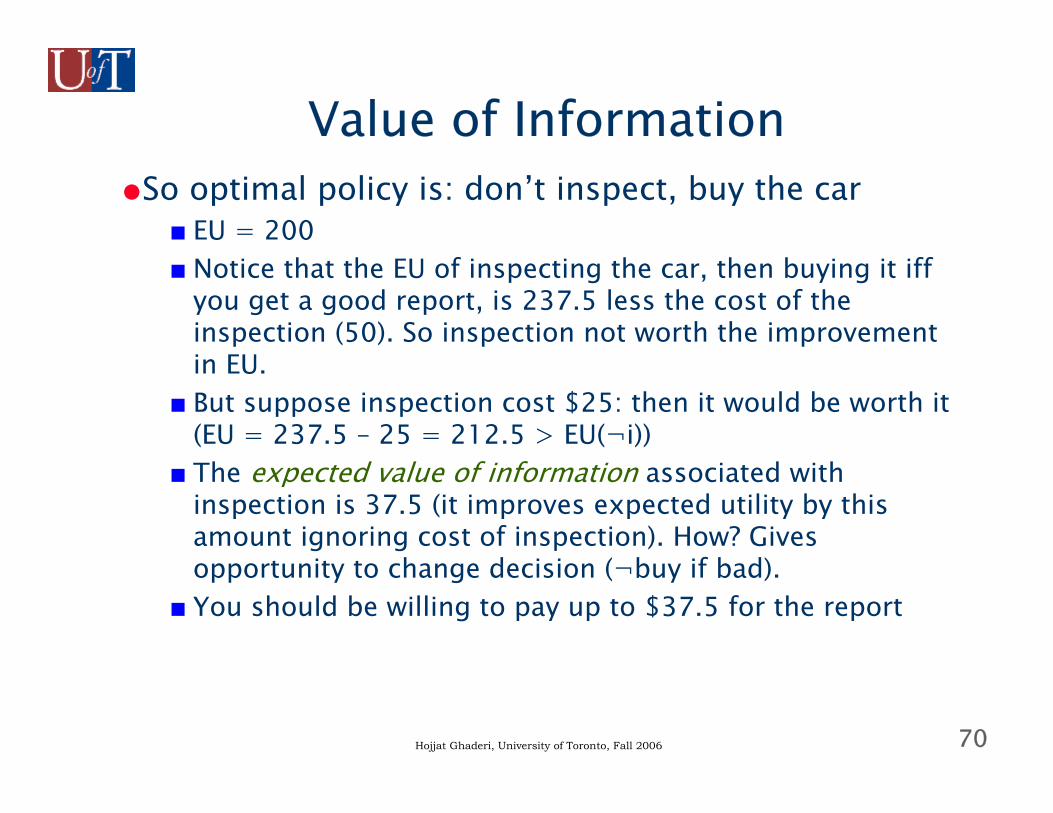
Value of Information●So optimal policy is: don’t inspect, buy the car

■ EU = 200■ Notice that the EU of inspecting the car, then buying it iff

you get a good report, is 237.5 less the cost of the inspection (50). So inspection not worth the improvement in EU.

■ But suppose inspection cost $25: then it would be worth it (EU = 237.5 – 25 = 212.5 > EU(¬i))

■ The expected value of information associated with inspection is 37.5 (it improves expected utility by this amount ignoring cost of inspection). How? Gives opportunity to change decision (¬buy if bad).

■ You should be willing to pay up to $37.5 for the report

csc384: intro to artificial intelligence decision making ...hojjat/384f06/lectures/lecture21.pdf ·...

Documents