csg water as a medium to grow marine …eprints.usq.edu.au/21946/1/harrington_2011.pdf · faculty...

University of Southern Queensland

Faculty of Engineering and Surveying

CSG WATER AS A MEDIUM TO GROW MARINE

MICROALGAE FOR BIOFUEL PRODUCTION

A dissertation submitted by

Daniel Harrington

in fulfilment of the requirement of

Course ENG4111 and 4112 Research Project

towards the degree of

Bachelor of Engineering (Civil)

Submitted: October, 2011

i

ABSTRACT

Over the next decade, the expanding Coal Seam Gas (CSG) industry in the Bowen and Surat

Basins is expected to produce between 50 to 300 GL of CSG water per year as a by-product of

its methane extraction processes. CSG water is high in sodium, salts, carbon in the form of

bicarbonates and other undesirable substances making it unfit for direct use.

Typically CSG water has been considered as a waste product, and is currently discharged in large

evaporation ponds. The QLD Government has recently introduced policy encouraging the

beneficial utilization of this water. Due to its high bicarbonate concentration, CSG water has the

potential to be used as a medium for growing microalgae for the production of biofuel.

Microalgae derived biofuel is one of the more promising alternate green energy fuel sources to

emerge in recent years. This method is superior to traditional crop based biofuels as it requires

substantially less water and land area to yield equivalent oil volumes. Furthermore, it has the

additional potential of cleansing nutrient rich waste waters.

Hence, the aim of this dissertation was to assess the potential of using CSG water as a medium

for growing microalgae to produce biofuel. Additionally, investigation was made of the carbon

sequestration and nutrient removal capacity of this process. Three sets of batch experiments

were conducted using a 3.5 L batch bio-reactor. In all trials, DO, pH and temperature were

monitored in real time, along with daily sampling of carbon, nitrogen and phosphorous to

calculate the depletion rates. Furthermore, algal growth was documented by measuring

suspended solids concentrations, and by optical density measurement using a spectrophotometer.

A preliminary set of trials were completed to validate the growth and monitoring capacity of the

bio-reactor. The trials inoculated microalgae Chlorella vulgaris in a controlled MBL media. A

florescent light source, compressed air and a CO2 feed were provided to facilitate algal growth.

The pH was set within the range 7.5±0.6. Trial results generally validated monitoring and

growth capacity using the installed bio-reactors.

ii

Trials were then conducted using the microalgae Dunaliella tertiolecta in a CSG water medium.

All trials were run for 5 days. The reactor was filled with 3L CSG water, inoculated with 250ml

Dunaliella tertiolecta, and 5ml/L of F2 concentrate was added to provide a nutrient source. The

bicarbonate level in the CSG water was increased to a mean concentration level (216 C mg/L),

through the addition of sodium bicarbonate (NaHCO3). The pH was controlled at a set point

7.6±0.5. A fluorescent light source was provided, and assessment was made of the effect of

aeration on algal growth and carbon stripping. Poor growth was recorded for non-aeration and

aeration scenarios, with initial growth rates of 0.0292 g SS/L/d and 0.0303 g SS/L/d,

respectively. Over the five day trial periods, algal carbon sequestration quantities of up to

90.9mg/L were achieved, and aeration was found to cause carbon stripping of up to 81.52 mg/L.

Nitrogen and phosphorous removal rates were 0.818mg N/L/d and 0.362 mg P/L/d for the non-

aeration trial, and 1.523 mg N/L/d and 0.381 mg P/L/d for the aeration trial. Nutrient depletion

P:N ratios of 1:2 to 1:4 were observed.

Due to the poor growth performance, identification was made of the optimal salinity level for

growth of Dunaliella Tertiolecta in CSG water (10 mg NaCl/L), trials were then repeated.

Results found high growth in the non-aeration and aeration trials, with growth rates of 0.0935 g

SS/L/d and 0.0808 g SS/L/d, respectively. Growth performance suggested no overall benefit in

adopting aeration for algal growth facilitation. Furthermore, carbon sequestration levels of up to

82.2mg/L were achieved, and carbon aeration was found to cause carbon stripping of up to 72.4

mg/L. Nitrogen and phosphorous removal rates were 2.335 mg N/L/d and 1.156 mg P/L/d for

the non-aeration trial, and 2.808 mg N/L/d and 0.959 mg/L/d for the aeration trial. Nutrient

depletion P:N ratios of 1:2 to 1:3 were observed. The algal dry mass and total lipid content of the

trials were 0.39 g and 24% for the non-aeration, and 0.41 g and 20% for the aeration trial.

The research suggest that the microalgae Dunaliella Tertiolecta has the potential to be grown in

CSG water, in an open pond settings, for biofuel production purposes. Trials found that the

microalgae Dunaliella Tertiolecta would grow in the CSG media, however increased salinity

levels of about 10 g/L were required to achieve optimal growth. This suggests that if the CSG

water is subjected to reverse osmosis treatment, then the resulting brine having a high

concentrated salinity could be used as an ideal medium to grow the desired algal strand. Further

analysis would be required to determine the economic viability of this process.

iii



ENG4111 Research Project Part 1 &

ENG4112 Research Project Part 2

Limitations of Use

The Council of the University of Southern Queensland, its Faculty of Engineering and

Surveying, and the staff of the University of Southern Queensland, do not accept any

responsibility for the truth, accuracy or completeness of material contained within or associated

with this dissertation.

Persons using all or any part of this material do so at their own risk, and not at the risk of the

Council of the University of Southern Queensland, its Faculty of Engineering and Surveying or

the staff of the University of Southern Queensland.

This dissertation reports an educational exercise and has no purpose or validity beyond this

exercise. The sole purpose of the course pair entitled “Research Project” is to contribute to the

overall education within the student's chosen degree program. This document, the associated

hardware, software, drawings, and other material set out in the associated appendices should not

be used for any other purpose: if they are so used, it is entirely at the risk of the user.

Professor Frank Bullen

Dean


iv

CERTIFICATION

I certify that the ideas, designs and experimental work, results, analyses and conclusions set out in this dissertation are entirely my own effort, except where otherwise indicated and acknowledged. I further certify that the work is original and has not been previously submitted for assessment in any other course or institution, except where specifically stated. Student Name Daniel Harrington Student Number: w0053544 ____________________________ Signature ____________________________ Date

v

ACKNOWLEDGMENTS

First and foremost I would like to thank Dr Vasanthadevi Aravinthan for her dedicated

supervision throughout the year. Without her enthusiastic and knowledgeable help, this project

would not have been as successful or as enjoyable. I would also like to thank Atul Sakhiya for

his continual help, and for coming into the university even on his days off to let me do some

sampling. Without his help this project would not have been as complete.

I also want to thank Saddam Hussen Allwayzy, Raed Ahmed Mahmood, Morwenna Boddington

and Adele Jones for their friendly and helpful assistance.

I would like to make a special mention to Cathy Johnston. Her assistance in the early stages of

this project to overcome some initial hurdles is very much appreciated.

My final thanks go to my family, and friends for their continual support throughout this project

and my time at university.

vi

CONTENTS

ABSTRACT .................................................................................................................................... i

CERTIFICATION ....................................................................................................................... iv

ACKNOWLEDGMENTS ............................................................................................................ v

LIST OF FIGURES ................................................................................................................... xiii

LIST OF TABLES ..................................................................................................................... xix

INTRODUCTION......................................................................................................................... 1

1.1 AIMS AND OBJECTIVES .............................................................................................. 2

1.2 SCOPE OF STUDY ......................................................................................................... 3

1.3 DISSERTATION OUTLINE ........................................................................................... 3

LITERATURE REVIEW ............................................................................................................ 5

2.1 MICROALGAE AS A FUEL SOURCE ......................................................................... 5

2.2 MICROALGAE BIOFUELS Vs CROP BASED BIOFUELS ........................................ 6

2.3 ADDITIONAL USES ...................................................................................................... 8

2.4 MICROALGAE BIOFUELS AS A VEHICLE FOR DECENTRALISATION AND

NATIONAL FUEL SECURITY ................................................................................................. 9

2.5 CSG WATER – PROPERTIES, ISSUES AND POTENTIALS ..................................... 9

2.6 MICROALGAE STRAND DUNALIELLA TERTIOLECTA ..................................... 12

2.7 CULTURING TECHNIQUES ....................................................................................... 13

2.7.1 LIGHT..................................................................................................................... 13

2.7.2 CARBON SUPPLY – C02 AND HCO3- ................................................................. 13

2.7.3 SALINITY .............................................................................................................. 14

2.7.4 AERATION ............................................................................................................ 14

vii

2.7.5 NUTRIENTS .......................................................................................................... 15

2.7.6 TEMPERATURE ................................................................................................... 15

2.8 GROWTH PHASES ...................................................................................................... 15

2.9 PHOTOSYNTHESIS ..................................................................................................... 16

2.10 ALGAL HARVESTING ................................................................................................ 17

2.11 CHAPTER SUMMARY ................................................................................................ 17

CHAPTER 3 METHODOLOGY ........................................................................................ 18

3.1 CULTURING OF MICROALGAE ............................................................................... 18

3.1.1 ALGAL STRAND DUNALIELLA TERTIOLECTA ........................................... 18

3.1.2 ALGAL STRAND CHOLERA VULGARIS ......................................................... 18

3.2 WATER COLLECTION AND PREPERATION .......................................................... 19

3.2.1 CSG WATER.......................................................................................................... 19

3.2.2 MBL MEDIA .......................................................................................................... 19

3.3 WATER CHARICTERISTICS AND NUTRIENT/BICARBONATE ADDITION ..... 19

3.3.1 CSG WATER.......................................................................................................... 19

3.3.2 CARBON ADDITION TO CSG WATER ............................................................. 20

3.3.3 F/2 CONCENTRATE ............................................................................................. 20

3.3.4 MBL MEDIA .......................................................................................................... 22

3.4 BIO-REACTOR DESIGN ............................................................................................. 22

3.4.1 INPUT VARIABLES ............................................................................................. 23

3.4.2 pH MONITORING AND CONTROLLING .......................................................... 24

3.4.3 DO AND TEMPERATURE MONITORING ........................................................ 24

3.4.4 LABVIEW PACKAGE .......................................................................................... 25

3.5 EXPERIMENTAL MEASUREMENTS ....................................................................... 26

3.5.1 MESUREMENT OF ALGAE GROWTH .............................................................. 26

viii

3.5.2 MEASUREMENT OF NUTRIENT DEPLETION & CARBON

SEQUESTRATION LEVELS ............................................................................................... 26

3.5.3 MEASUREMENT OF DO AND pH DATA.......................................................... 27

3.6 MICROALGAE HARVEST .......................................................................................... 28

3.6.1 MEASUREMENT OF ALGAL DRY WEIGHT ................................................... 29

3.7 LIPID EXTRACTION AND ANALYSIS ..................................................................... 30

3.8 DATA ANALYSIS ........................................................................................................ 30

3.8.1 CARBON AND NUTRIENT UTILIZATION CALCULATIONS ....................... 30

3.8.2 NITRONGEN CONCENTRATION ADJUSTMENT OF CHORELLA

VULGARIS TRIALS ............................................................................................................ 31

3.8.3 CONCENTRATION ADJUSTMENT FOR DUNALIELLA TERTIOLECTA

TRIALS 32

3.8.4 SPECIFIC GROWTH RATE CALCULATIONS .................................................. 32

3.8.5 DATA MANIPULATION ...................................................................................... 33

3.9 RISK MANAGEMENT ................................................................................................. 33

3.9.1 WORKING WITH HAZARDS CHEMICALS ...................................................... 33

3.9.2 DISEASE PREVENTION ...................................................................................... 34

3.9.3 DISPOSAL METHOD OF BIOHAZARD MATERIALS ..................................... 34

3.9.4 RISKS BEYOND COMPLETION OF THE PROJECT ........................................ 34

3.10 CHAPTER SUMMARY ................................................................................................ 34

CHAPTER 4 GROWTH CHARICTERISTICS OF MICROALGAE CHLORELLA

VULGARIS GROWN IN MBL MEDIA AND THE EFFECTS OF CO2 INPUT. .............. 35

4.1 BATCH EXPERIMENTS .............................................................................................. 35

4.1.1 EXPERIMENT 1 (MBL MEDIA – CO2 ADDITION) .......................................... 35

4.1.2 EXPERIMENT 2 (MBL MEDIA – NO CO2 ADDITION) .................................... 36

4.2 ALGAL GROWTH ........................................................................................................ 36

ix

4.2.1 EXPERIMENT 1: GROWTH CHARICTERISTICS ............................................. 36


4.2.3 ALGAL GROWTH SUMMARY ........................................................................... 40

4.3 pH VARIATION ............................................................................................................ 41

4.3.1 EXPERIMENT 1: pH VARIATION ...................................................................... 41


4.4 DISSOLVED OXYGEN VARIATION ........................................................................ 45

4.4.1 EXPERIMENT 1: DO VARIATION ..................................................................... 45


4.5 NUTRIENT REMOVAL ............................................................................................... 49

4.6 ALGAE DRY MASS AND LIPID CONTENT ............................................................ 51

4.7 ENCOUNTED PROCEDURAL ISSUES ..................................................................... 51

4.7.1 pH VOLATILITY ................................................................................................... 51

4.7.2 ALGAL SETTLEMENT AND CLUMPING ......................................................... 51

4.8 CONCLUSIONS ............................................................................................................ 52

CHAPTER 5 GROWTH CHARICTERISTICS AND LIPID PRODUCTION OF

MICROALGAE DUNALLIELLA TERTIOLECTA GROWN IN A CSG W ATER MEDIA

AND THE EFFECTS OF AERATION. ................................................................................... 53


5.1.1 EXPERIMENT 1 (CSG WATER MEDIA – NON-AERATION) ......................... 53

5.1.2 EXPERIMENT 2 (CSG WATER MEDIA – AERATION) ................................... 54

5.2 ALGAL GROWTH ........................................................................................................ 54




5.3 CARBON SEQUESTRATION ..................................................................................... 58

x

5.3.1 EXPERIMENTS 1 & 2: CARBON LEVELS ........................................................ 58

5.3.2 CONTROL TRIAL: CARBON LOSS ................................................................... 59

5.3.3 CARBON SEQUESTION ASSESSMENT ............................................................ 59


5.4.1 NITROGEN REMOVAL ....................................................................................... 60

5.4.2 PHOSPHOROUS REMOVAL ............................................................................... 61

5.5 pH VARIATION ............................................................................................................ 62



5.5.3 pH VARIATION SUMMARY ............................................................................... 66




5.6.3 DISSOLVED OXYGEN MEASUREMENT SUMMARY ................................... 71




5.8.2 POOR GROWTH RESULTS FOR DUNALIELLA TERTIOLECTA IN CSG

WATER 71

5.9 CONCLUSIONS ............................................................................................................ 71

CHAPTER 6 GROWTH CHARICTERISTICS AND LIPID PRODUCTION OF

MICROALGAE DUNALLIELLA TERTIOLECTA GROWN IN SALINIT Y MODIFIED

CSG WATER MEDIA AND THE EFFECTS OF AERATION. ...... ..................................... 73

6.1 OPTIMAL SALINITY IDENTIFICATION .................................................................. 73


xi

6.2.1 EXPERIMENT 3 (SALINITY MODIFIED CSG WATER MEDIA – NON-

AERATION) ......................................................................................................................... 74

6.2.2 EXPERIMENT 4 (SALINITY MODIFIED CSG WATER MEDIA – AERATION)

75

6.3 ALGAL GROWTH ........................................................................................................ 75



6.3.3 LOW BICARBONATE CONTROL TRIAL ......................................................... 78


6.4 CARBON SEQUESTRATION ..................................................................................... 80

6.4.1 EXPERIMENTS 3, 4 AND CONTROL TRIAL: CARBON LEVELS ................. 81

6.4.2 CARBON SEQUESTION ASSESSMENT ............................................................ 82


6.5.1 NITROGEN REMOVAL ....................................................................................... 83

6.5.2 PHOSPHOROUS REMOVAL ............................................................................... 83

6.6 pH VARIATION ............................................................................................................ 84



6.6.3 pH VARIATION SUMMARY ............................................................................... 88




6.7.3 DISSOLVED OXYGEN MEASUREMENT SUMMARY ................................... 93




xii

6.10 CONCLUSIONS ............................................................................................................ 94

CHAPTER 7 CONCLUSIONS AND FUTURE WORK .................................................. 95

7.1 CONCLUSIONS ............................................................................................................ 95

7.2 SUGGESTIONS FOR FUTURE WORK ...................................................................... 96

7.2.1 CLOSED LOOP AERATION SYSTEM ............................................................... 96

7.2.2 OPTIMAL BICARBONATE LEVEL IDENTIFICATION ................................... 97

7.2.3 ALTERNATE AGLAL STRAND ASSESSMENT ............................................... 97

7.2.4 IMPROVED pH CONTROL .................................................................................. 97

7.2.5 IMPROVED REACTOR DESIGN ........................................................................ 97

7.2.6 FUTURE EXPERIEMENTS .................................................................................. 98

7.3 SUMMARY ................................................................................................................... 98

REFERENCES ......................................................................................................................... 99

APPENDIX A PROJECT SPECIFICATION

APPENDIX B GROWTH AND NUTRIENT DEPLETION DATA SAMPL E

APPENDIX C MATLAB CODE SAMPLE

xiii

LIST OF FIGURES

Figure 2.1 Microalgae Dunaliella tertiolecta a) (EOL 2011), b) (CSIRO 2011). .................12

Figure 2.2 Algal growth phases and nutrient depletion rates for batch experiments .............16

Figure 3.1 Schematic diagram of the Bio-reactor setup .........................................................24

Figure 3.2 The Bio-reactor setup .............................................................................................24

Figure 3.3 Jenway 6705 UV/Vis Spectrometer output and filter paper samples for 12 day

period ....................................................................................................................26

Figure 3.4 Labview software output logging DO, pH, temperature and acid/base addition in

real time. ..............................................................................................................28

Figure 3.5 Beckman Avanti CentrifugeJ-25 I, Eppendorf Centrifuge 5810 R and VirTis

2KBTES-55 Freeze Dryer. ....................................................................................29

Figure 4.1 Experiment 1 – Algal growth in MBL media with CO2 addition measured with

Optical Density at 505 NM and Suspended Solids ................................................37

Figure 4.2 Experiment 1 - Relationship between Suspended Solids and Optical Density at

505NM. ..........................................................................................................................................37

Figure 4.3 Experiment 2 - Algal growth in MBL media without CO2 addition measured with

Optical Density at 505 NM and Suspended Solids. ..............................................38

Figure 4.4 Experiment 2 - Relationship between Suspended Solids and Optical Density at

505nm ....................................................................................................................39

Figure 4.5 Daily photos of algae growth in the Bioreactor for Experiment 2, documenting all

5 stages of growth. .................................................................................................39

xiv

Figure 4.6 Experiment 1 & 2 – Comparison of algal growth in MBL media with and without

CO2 addition measured with Optical Density (Experiment 1, Experiment 2) at 505

nm and Suspended Solids (Experiment 1, Experiment 2) .....................................40

Figure 4.7 Experiment 1 – Bioreactor pH readings for the 23 day trial. .................................42

Figure 4.8 Experiment 1 – Bioreactor pH readings over a 24 hr period for Day 1, 3 and 15 .43

Figure 4.9 Experiment 2 – Bioreactor pH readings for the 14 day trial .................................44

Figure 4.10 Experiment 1 – Bioreactor pH readings over 24 hr period for different growth

phases; Linear Phase, Stationary Phase and Death Phase ......................................45

Figure 4.11 Experiment 1 – Bioreactor DO readings for the 23 day trial .................................46

Figure 4.12 Experiment 1 –Average maximum DO readings during the light period, average

minimum DO readings during the dark period, net oxygen produced during the

light period and optical density reading .................................................................47

Figure 4.13 Experiment 1 – Daily oxygen quantities produced during the light period ...........47

Figure 4.14 Experiment 2 – Bioreactor DO readings for the 14 day trial .................................49

Figure 4.15 Experiment 2 –Average maximum DO readings during the light period, average

minimum DO readings during the dark period, net oxygen produced during the

light period and optical density reading .................................................................49


Figure 4.17 Experiment 1 – Nutrition removal rate measured through nitrogen depletion and

optical density growth measurements ....................................................................50

Figure 4.18 Experiment 1 – Nutrition removal rate measured through nitrogen depletion and

suspended solids growth measurements ...............................................................50

Figure 4.19 Algal clumping on the DO probe ..........................................................................51

xv

Figure 5.1 Experiment 1 – Algal growth in CSG water media without aeration addition

measured with Optical Density at 505 nm. ............................................................55

Figure 5.2 Experiment 1 – Algal growth in CSG water media without aeration measured with

derived Suspended Solids readings for first 4 days of the trial .............................55

Figure 5.3 Experiment 2 - Algal growth in CSG water media with aeration addition

measured with Optical Density at 505 nm. ...........................................................56

Figure 5.4 Experiment 2 – Algal growth in CSG water media with aeration addition

measured with derived Suspended Solids readings for first 4 days of trial ..........56

Figure 5.5 Experiment 1 & 2 – Comparison of algal growth in CSG water media with and

without O2 addition measured with Optical Density (Experiment 1, Experiment 2)

at 505 nm ...............................................................................................................57

Figure 5.6 Photographic comparison of algae growth in the Bioreactor for Experiments 1 and

2 over a 6 day trial period. .....................................................................................58

Figure 5.7 Total Carbon (TC) readings for (a) Experiment 1 and (b) Experiment 2 ..............59

Figure 5.8 Experiment 1, Experiment 2 and Control Trial – Carbon Depletion Rates

(Experiment 1, Experiment 2 and Control Trial) ...................................................60

Figure 5.9 Nitrogen readings for (a) Experiment 1and (b) Experiment 2 ...............................61

Figure 5.10 Phosphate readings for (a) Experiment 1 and (b) Experiment 2 ............................61

Figure 5.11 Experiment 1 – Bioreactor pH readings for the 5 day trial ....................................63

Figure 5.12 Experiment 1 – Bioreactor pH readings over a 24 hour period for Day 1, Day 2,

Day 3 and Day 4 ....................................................................................................64

Figure 5.13 Experiment 2 – Bioreactor pH readings for the 6 day trial ....................................65

Figure 5.14 Experiment 1 – Bioreactor pH readings over 24 hour period for Day 1, Day 2,

Day 3 and Day 4 ....................................................................................................66

xvi

Figure 5.15 Experiment 1 – Bioreactor DO readings for the 6 day trial. ..................................67

Figure 5.16 Experiment 1 –Average maximum DO readings during light period, average

minimum DO readings during dark period, Net oxygen produced during the day

time and Optical Density results ............................................................................68


Figure 5.18 Experiment 2 – Bioreactor DO readings for the 6 day trial ...................................69



time and Optical Density results ...........................................................................70


Figure 6.1 Algal growth in CSG water media measured with Optical Density at 505 nm with

salinity levels of 3.5 mg NaCl/L, 10 mg NaCl/L, 20 mg NaCl/L and 35 mg

NaCl/L....................................................................................................................74

Figure 6.2 Experiment 3 – Algal growth in salinity modified CSG water media without O2

addition measured with Optical Density at 505 nm ...............................................76

Figure 6.3 Experiment 3 – Algal growth in salinity modified CSG water media without O2

addition measured with derived Suspended Solids readings .................................76

Figure 6.4 Experiment 4 - Algal growth in salinity modified CSG water media with aeration

measured with Optical Density at 505 nm ............................................................77

Figure 6.5 Experiment 4 – Algal growth in salinity modified CSG water media with O2

addition measured with derived Suspended Solids readings ................................77

Figure 6.6 Experiment 3, 4 & Low Bicarbonate Control Trial – Comparison of Dunaliellla

tertiocleta growth in a salinity modified CSG water media measured with Optical

Density readings (Experiment 3, Experiment 4 and Low Bicarbonate Control

Trial) at 505 nm ....................................................................................................78

xvii

Figure 6.7 Experiment 1, 2, 3 and 4 – Comparison of Dunaliella tertiolecta growth in CSG

water with salinity levels 3.5 mg NaCl/L (Experiment 1 & Experiment 2) and 10

mg NaCl/L (Experiment 3 and Experiment 4) measured with Optical Density

readings at 505 nm ...............................................................................................79

Figure 6.8 Photographic comparison of algae growth in the Bioreactor for Experiments 3,

Experiment 4 and the Low Carbon Control Trial over a 6 day trial period. ..........80

Figure 6.9 a) Total Carbon (TC) readings for Experiment 3 .......................................................81

Figure 6.9 b) Total Carbon (TC) readings for Experiment 4 .......................................................81

Figure 6.9 c) Total Carbon (TC) readings for the Low Bicarbonate Control Trial .....................82

Figure 6.10 Experiment 1, Experiment 2, Carbon Loss Control Trial and Low Bicarbonate

Control Trial – Carbon Depletion Rates (Experiment 1, Experiment 2, Carbon

Loss Control Trial and Low Bicarbonate Control Trial) .......................................82

Figure 6.11 Nitrogen readings for (a) Experiment 3 and (b) Experiment 4 ..............................83

Figure 6.12 Phosphate readings for (a) Experiment 3 and (b) Experiment 4 ............................84

Figure 6.13 Experiment 3 – Bioreactor pH readings for the 5 day trial ...................................85

Figure 6.14 Experiment 3 – Bioreactor pH readings over a 24 hour period for Day 1, 2 and 4

........................................................................................................................................................86

Figure 6.15 Experiment 4 – Bioreactor pH readings for the 5 day trial. ...................................87

Figure 6.16 Experiment 4 – Bioreactor pH readings over 24 hour period for Day 1, 2 and 3 ..88

Figure 6.17 Experiment 4 – Bioreactor DO readings for the 5 day trial. ..................................89



time and Optical Density results. ...........................................................................90

Figure 6.19 Experiment 3 – Daily oxygen quantities produced during the light periods .........91

xviii

Figure 6.20 Experiment 4 – Bioreactor DO readings for the 5 day trial ...................................91



time and Optical Density results. ...........................................................................92

Figure 6.22 Experiment 4 – Daily oxygen quantities produced during the light periods ........92

xix

LIST OF TABLES

Table 2.1 Comparison of some biofuel sources (Chisti 2007) .................................................7

Table 2.2 Comparison of Greenhouse gas emissions over biofuel life cycle for popular

biofuel crops (Groom et al. 2008) ............................................................................8

Table 2.3 CSG water quality statistics within a single field in the Bowen Basin grouped

according to seam and position relative to fault (Kinnon et al. 2010) ...................10

Table 2.4 Input/output estimates of a 900 ha pond managing 10GL of CSG water per year

(Pratt et al. 2011)....................................................................................................12

Table 3.1 Composition of CSG Water sample ......................................................................20

Table 3.2 Composition of CSG Water sample (plus 1mg/L of F2 concentrate) ....................21

Table 3.3 Composition of MBL media .................................................................................22

Table 6.1 Algal dry mass and lipid content ...........................................................................93

1

INTRODUCTION

The expected increases in world energy usage in the coming years, means that a number of new

green renewable energy sources must be developed to meet future demands and to reduce

greenhouse gas emissions (Mata et al 2010). In Australia, approximately 75% of transport fuel

comes from local oil and gas sources. It is predicted that this market portion could reduce to

45% by 2030 with growing national demand, and without any new discoveries or technological

breakthroughs (CSIRO 2011). Alternate methods of fuel production will need to be developed

and or expanded in the coming years to limit the potential of future foreign fuel source

dependency, and to ensure national fuel security.

Currently, the prominent alternate to fossil fuels is crop based biofuel, accounting for

approximately 2% of the domestic fuel market (Australian Treasury 2011). This production

method has limitations however, it is not sustainable and it competes with the agricultural

industry for farmable land. Microalgae derived biofuels offer an alternative that overcomes these

limitations. This fuel production method requires significantly less land area, does not need

arable land and can utilize saltwater, brackish water or wastewater for production. Conservative

estimates by the CSIRO, based on an algal oil content of 20%, states that a pond area of

10,000km2 would be required to produce enough microalgae biofuel to meet Australia’s current

domestic demand needs. Alternately, a farmable area of 1,320,000 km2 (17% of Australia’s land

mass) and a fresh water supply would be required to produce the same oil yield using a soy bean

crop, which is one of the more popular biofuel crops. This disparity highlights both the

limitations of traditional methods and the potential of microalgae biofuels.

The utilization of Coal Seam Gas (CSG) water as a medium for microalgae biofuel production

presents one opportunity for the creation of a new carbon neutral fuel source. CSG water, a by-

product of the CSG extraction process, is considered as a waste material and is typically disposed

of in large evaporation ponds. This water is rich in carbon in the form of bicarbonates.

Optimal algal production, requires a source of carbon, this generally is supplied by a CO2 feed

from industry or power stations. This project differentiates in that the carbon source is pre-

2

existing in the CSG water. Therefore there is the potential to use existing open pond

infrastructure for algal growth, without the need to develop a CO2 feed method. There are

several other potential benefits in using CSG water for biofuel production, including offsetting

carbon emissions by replacing fossil fuel products, generating new industry in rural areas and

assisting in decentralising fuel production.

With no current published research pertaining to algal growth for biofuel production in a CSG

water media, this dissertation was intended as a preliminary investigation to evaluate the

feasibility of this process. Assessment will be made by conducting lab scale batch experiments

growing a marine algae (Dunaliella tertiolecta) in a CSG water media. A critical analysis will

be made of the algal growth, carbon sequestration, nutrient removal and oil production capacity

of this process.

1.1 AIMS AND OBJECTIVES

The aim of this project is to assess the potential of growing microalgae Dunaliella tertiolecta in a

Coal Seam Gas water media, for the purpose of producing biofuel. Determination of the carbon

sequestration and nutrient removal capacity of this process will also be assessed.

The objectives of the research were to:

• Obtain a CSG water sample and test for nutrient and chemical composition

• Conduct batch experiments with microalgae Dunaliella tertiolecta in CSG water and

simultaneously measure

o algal growth

o pH variation

o dissolved oxygen variation

o carbon variation

o nutrient variation (supplemented nitrogen and phosphorous)

• Identify optimal salinity levels for algal growth

• Identify algal growth, pH and DO patterns

• Measure carbon and nutrient depletion rates

• Harvest the algae and measure total lipid production

3

1.2 SCOPE OF STUDY

The scope of this study is to identify the potential of undertaking biofuel production, carbon

sequestration and nutrient removal, using Dunaliella tertiolecta in a CSG water medium.

Limitations of this research were:

• Only one algal strand was tested in CSG water

• All batch experiments were only conducted once

• Assessment could not be made of the quantities and removal rates of trace elements

• While most of the inputs and outputs could be assessed, the chemical and biological

reactions within the system could not be described. Essentially the system represented a

black box.

1.3 DISSERTATION OUTLINE

Chapter 2 Literature Review

This chapter reviews and summarises the current literature pertaining to beneficial uses of

microalgae, culturing techniques and algal growth phases. The properties and issues of CSG

water in Queensland are evaluated. And a brief overview of photosynthesis and the resulting DO

and pH fluctuations is provided.

Chapter 3 Methodology

This chapter provides an overview of the methodology used to analysis wastewater

characteristics, microalgae growth patterns, carbon and nutrient depletion rates and lipid content.

It also demonstrates how the experimental equipment was set up, and reviews the equipment

used.

Chapter 4 Growth Characteristics of Microalgae Chlorella vulgaris Grown in MBL Media

and the effects of CO2 input.

This chapter presents the results relating to the testing of microalgae Chorella vulgaris grown in

MBL media. It shows growth patterns, pH fluctuations, dissolved oxygen variability and

nitrogen removal. This chapter also assesses the effect of CO2 feed on algal growth.

4

Chapter 5 Growth Characteristics of Microalgae Dunaliella tertiolecta Grown in a CSG

Water Media and the Effects of Aeration

This chapter presents the results relating to the testing of microalgae Dunaliella tertiolecta

grown in a CSG water medium. It shows growth patterns, carbon sequestration, nutrient

removal, pH fluctuations and dissolved oxygen variability. This chapter also assesses the effect

of aeration on algal growth.

Chapter 6 Growth Characteristics and Lipid Production of Microalgae Dunaliella

tertiolecta Grown in Salinity Modified CSG Water Media and the Effects of

Aeration

This chapter presents the results relating to the testing of microalgae Dunaliella tertiolecta

grown in a salinity modified CSG water medium. It shows growth patterns, carbon

sequestration, nutrient removal, pH fluctuations and dissolved oxygen variability. This chapter

also assesses the effect of aeration on algal growth and evaluates lipid extraction results.

Chapter 7 Conclusions and Future Works

This chapter presents the conclusions of the study and reviews future works.

5

LITERATURE REVIEW

The literature review covers the topic of biofuel, and compares traditional crop methods with

microalgae biofuels. Assessment is made of CSG water, and its potential utilisation. In addition,

an overview of microalgae Dunaliella tertiolecta, algal culturing techniques and reactions

involving photosynthesis are provided.

2.1 MICROALGAE AS A FUEL SOURCE

The oil sector accounts for approximately 35% of the global energy market (Lin et al. 2010).

With increasing crude oil prices and limitations on future reserves, coupled with a conscious

public and political shift towards reducing carbon emissions, huge opportunities are now

emerging for greener renewable fuel sources. Biofuels including biodiesel, bioethanol and

biomethane represent a viable alternative to petroleum. These fuels are theoretically carbon

neutral, renewable, and can generally be applied as a blend or direct substitute for petroleum,

with little or no modification to modern vehicle engines (Mata 2010).

It is expected that the global biofuel industry will increase rapidly, to a value of over US $500bn

by 2050 (Stern 2007). In Australia biofuel currently accounts for only 2% of the national fuel

market. However the federal treasury department predicts that the inclusion of heavy vehicle

fuel usage into the impending carbon tax legislation will drive significant investment and

development into the biodiesel industry. Modelling by the department suggests that biodiesel

usage will become the dominant fuel source for heavy vehicles by 2030, and it will represent

over 75% of the market by 2050. The department further states that the transition to a biofuel

market will occur regardless of a carbon tax (Federal Treasury Department 2011).

Biofuels are produced predominantly from plant matter. Essentially the production process

entails growing plant matter which converts solar energy into chemical energy through

photosynthesis. This chemical energy in the form of fats, sugars and oils is then extracted

through various processes to create a usable fuel source. Traditional biofuels are produced using

6

higher order plant crops, with the most popular crops including corn, soy bean, canola and

rapeseed (Singh & Gu 2010).

Microalgae derived biofuels have recently emerged as a potential fuel source able to overcome

many of the environmental and economic limitations of traditional biofuel methods.

Fundamentally this process replaces higher order plant crops with microalgae as the biomass for

fuel production. Microalgae have an extractable oil content of between 10% and 80%, with oil

contends of 20% to 50% being the most common (Chisti 2007). Oil content is dependent on the

algal strand and the set growing conditions.

2.2 MICROALGAE BIOFUELS Vs CROP BASED BIOFUELS

Fuel derived from higher order plants is currently the most common form of biofuel production

globally (Schneck etal. 2008). This method is problematic for two main reasons, the limitations

of arable land availability and the developing competition with food production industries for

feedstock acquisition.

Crop based biofuels could not be considered as a future substitute to petroleum fuels, as the

arable land area required to meet fuel demand needs, is at best unsustainable and at worst

unachievable. Table 2.1 shows a comparison of some of the more popular biofuel crop types,

and their oil yield per hectare ratios. Also shown, are estimates of the land areas required to

meet 50% of the USA’s current fuel demand, and the equivalent percentage of existing crop area

in the USA (Chisti 2007). Results clearly demonstrate the limitations of traditional crop

methods. In Australia it is conservatively estimated that 1 million hectares or 0.13% of the

nation’s total land area would be required to produce enough algae (20% oil content) to meet all

of the current domestic fuel demand needs (CSIRO 2011).

An additional concern with traditional crop based biofuel production, is the potential that

existing rainforest and ecologically significant areas, particularly in developing countries, could

be lost as a result of increased pressures for cultivation of biofuel cash crops (Mata, 2011).

7

TABLE 2.1 Comparision of some biofuel sources (Chisti 2007)

Crop Oil yield

(L/ha)

Land area to meet

50% of USA fuel

demand (million ha)

Equivalent precent

of existing USA

cropping area (%)

Corn 1540 1540 846

Soybeans 594 594 326

Canola 1190 223 122

Jatropha 1892 140 77

Coconut 2689 99 54

Oil Palm 5950 45 24

Microalgae (70% oil) 136,900 2 1.1

Microaglae (30% oil) 58,700 4.5 2.5

The second major limitation of traditional biofuel methods is that it competes directly with

agricultural industries for arable land usage. Over 75% of the cost associated with producing

crop based fuels comes from the acquisition of feedstock (Schneck etal. 2008). As traditional

biofuel production expands, so does the industry’s demand for additional feedstocks, which in

turn leads to greater competition between food and biofuel producers for land use, driving up

prices for both forms of industry. Crop based bio-fuel production has increased tenfold from

2000 to 2008, and since 2002 a strengthening correlation has been observed between world food

prices and biodiesel production (L Lin et al. 2011). Shortages and subsequent increases in prices

of food stocks can have, and has had major detrimental effects on a global scale. Recent food

price rises have been linked civil unrest in northern and western Africa (L Lin et al. 2011).

Microalgae biofuels have the advantage in that they do not require fertile or productive lands for

cultivation and they use much less area and water for equivalent yields of oil (Harun et al 2011).

The algae strands used for these fuels typically require water, sunlight, CO2, O2, and key

nutrients potassium and nitrogen (Schneck etal. 2008). Additionally there is the capacity for

algae to be farmed in saltwater or brackish, thereby reducing dependency on limited fresh water

supplies (Singh & Gu 2010).

8

2.3 ADDITIONAL USES

There are a number of products that can be produced from alga. Including food and nutrient

supplements, organic fertilisers, livestock feed and fine organic chemicals for pharmaceutical

goods (Singh & Gu 2010). Furthermore, as microalgae have a greater capacity for

photosynthesis than higher plants, there is much potential to utilize this organism for offsetting

CO2 emissions (Fernandes 2010). Table 2.2 shows the Greenhouse gas emissions over the

biofuel life cycle for microalgae and other popular biofuel crops. As a comparison, the rates for

gasoline and diesel are 94 kg CO2/MJ and 83 kg CO2/MJ, respectively (Groom et al. 2008). The

high negative net carbon output rate for microalgae (-183 kg CO2/MJ) demonstrates the

sequestration potential of this process.

TABLE 2.2 Comparison of Greenhouse gas emissions over biofuel life

cycle for popular biofuel crops (Groom et al. 2008)

Crop GHG emissions (kg CO2/MJ)

Corn 81 to 85

Soybeans 49

Canola or Rapeseed 37

Oil Palm 51

Sugar Cane 4 to 12

Native prairie grasses -88

Microalgae (Biodiesel) -183

There is also the potential to combine algal biofuel production with water cleaning processes.

Nutrient rich industry wastewater can be used as a feedstock for algae biofuel production, algae

have the capacity to absorb and remove nutrients from wastewater. The treatment of wastewater

can be costly for industries, by combining water treatment with bio-fuel production, there is the

capacity to turn a waste cost into a profitable resource (SARDI 2010).

Another production alternately, is to use the biomass waste remaining after lipid extraction to

produce biogas through anaerobic digestion. Harun et al (2011) suggest that production cost and

carbon emission from biofuel production systems could theoretically be reduced by 33% and

75% respectively through the integration of biodiesel production with biogas production.

9

2.4 MICROALGAE BIOFUELS AS A VEHICLE FOR

DECENTRALISATION AND NATIONAL FUEL SECURITY

The decentralisation of energy distribution is generally recognised as a more efficient, reliable

and environmentally friendlier method for delivering energy, compared to the traditional

centralised distribution method (Alanne & Saari 2005). Through this process, large energy

conversion units are replaced by smaller ones, with the capacity to be located closer to energy

consumers. Microalgae biofuel production can be easily applied to a decentralisation model, as

there is capacity at most wastewater and carbon emitting facilities to generate this fuel source.

Furthermore, a microalgae biofuel market has the potential to provide a secure national fuel

source. In Australia approximately 75% of transport fuel comes from local sources, however

with growing demands and source limitations, this market portion could reduce to 45% by 2030

(CSIRO 2011). Therefore alternate fuel sources must be developed to avoid future dependency

on foreign fuel importation. Algal derived biofuels have the capacity to be produced year round

and can be harvested daily, ensuring a steady oil supply.

2.5 CSG WATER – PROPERTIES, ISSUES AND POTENTIALS

The Coal Seam Gas (CSG) industry has grown substantially in Queensland over the last decade.

Encouraged through the State Governments “Queensland Energy Policy – A Cleaner Energy

Strategy”, the production of CSG increased from 4PJ in 1998-1999 to 125PJ in 2007-2008. In

2010 it comprised over 80% of Queensland’s gas market. Despite the significant grow to date it

is still considered a new industry with major expansion expected (Kinnon 2010).

The CSG extraction method involves drilling wells into coal seams and pumping the water from

these wells to reduce pressure within the matrix that acts to contain the methane gas in the coal.

This causes methane to desorb and begin to flow from the coal, gas and water then travel

together to the surface where they are then separated (Kinnon 2010). Through this process, large

quantities of CSG water is produced. Current estimates for CSG water to be generated from

Queensland’s Surat and Bowen Basins over the next decade range from 50 to 300GL per year

(Pratt et al 2011).

10

CSG water contains variable levels of sodium, salts, carbon in the form of bicarbonates and

several trace elements, making it unfit for direct use. Table 2.3 shows water quality sampling

results from various well depths and locations within a single field in the Bowen Basin.

Comparison is made with the chemical composition of seawater.

TABLE 2.3 CSG water quality statistics within a single field in the Bowen Basin grouped according to

seam and position relative to fault (Kinnon et al. 2010)

Upper seam

north of

fault

Upper seam

south of

fault

Upper seam

north of

fault

Lower seam

north of fault

Seawater

Depth (m) 273 177 333 228

pH 7.9 7.9 8 7.8 8.1

Electrical Conductivity

at 25°C (S/m)

10,570 7,865 8,645 11,140

TDS at 180°C (ppm) 5,810 4,488 4,838 5,846 35,000

Hydroxide alkalinity as

CaCO3 (mg/L)

<1 <1 <1 <1

Carbonate alkalinity as

CaCO3 (mg/L)

25 4 12 <1

Bicarbonate alkalinity

as CaCO3 (mg/L)

719 667 1,482 550

Total alkalinity as

CaCO3 (mg/L)

727 670 1,494 550

Sulphate as SO2-4 (mg/L) <1 <1 <1 1

Cl (mg/L) 3,280 2,330 2,223 3,670 19,700

Ca (mg/L) 40 46 15 52 410

Mg (mg/L) 23 16 9 26 1310

Na (mg/L) 2,423 1,730 2,054 2,464 1,900

K (mg/L) 17 10 8 12 390

Fe (mg/L) 5.46 5.30 5.37 5.14 <0.02

Al (mg/L) 0.06 0.36 0.07 0.04 <0.01

F (mg/L) 1.3 1.8 2.4 1.6 1.4

11

Typically CSG water has been disposed of in large evaporation ponds, it is essentially considered

a waste product. In October 2008 the Queensland Government released the Queensland Coal

Seam Gas Water Management Policy, which outlined the strategy for CSG water management.

Central to the policy was the discontinuation of evaporation ponds as the primary means of CSG

water disposal. A 3 year transitional period was allocated for the remediation of existing open

ponds. In June 2010 DERM implemented the Coal Seam Gas Water Management Policy. This

policy states that the preferred management options for CSG water utilization was either through

augmenting depleted natural aquifers, through direct use methods or through treatment methods

for varying application. The purpose of the DERM policy is twofold to ensure that CSG water

does not contaminate the environment, and to encourage the beneficial use of CSG water.

The policy further states that, an alternate use approval can be granted where CSG water is

converted from a waste to a resource that can be used for beneficial purposes (DERM 2010).

This paper examines the potential to utilise this carbon rich CSG water for algae biofuel

production purposes. Potential benefits include creating industry in rural areas, aiding to

decentralise fuel production sources and create a net CO2 offset by replacing fossil fuels and

other carbon intensive products with alga derived products.

Table 2.4 shows estimates by Pratt et al. (2011), of the production and profit generation potential

of algal derived products grown in a CSG water medium with a nutrient waste supplement, also

estimated is the carbon capture and offset capacity of this process. Estimates have been based on

conceptual 900 ha pond design, managing 10 GL of CSG water per year and incorporating

agricultural waste inputs to produce biodiesel, methane and biosolid products.

12

TABLE 2.4 Input/output estimates of a 900 ha pond managing 10GL of CSG water per

year (Pratt et al. 2011)

Product Volume Value

Algae 108,000 t

Water 10 GL

Biodiesel 24,000 m3 $24 M

Methane 891, 000 GJ $ 6.2 M

Biosolids 45,000 t DS $1.13

CO2 capture and off-sett

Capture in algae biomass 206,000 t

Off-set via biodiesel 58,500 t $1.17 M

Off-set via methane 54,000 t $1.08 M

2.6 MICROALGAE STRAND DUNALIELLA TERTIOLECTA

The microalgae Dunaliella tertiolecta (Figure 2.1 a & b) is a unicellular green marine alga, 9-

11µm in size. This alga has a reported oil yield of 36%-42%. It is simple to cultivate, fast

growing, does not clump or form chains, and it can be grown in saltwater, wastewater or

brackish water (Chen et al 2011). As such Dunaliella tertiolecta is an ideal candidate for

application in an untested medium. Should the lab scale experiments using Dunaliella tertiolecta

prove successful, there is the future potential to use this algal strand in large outdoor pond

settings.

a) b)

FIGURE 2.1 Microalgae Dunaliella tertiolecta. a) (Encyclopaedia of Life 2011), b) (CSIRO 2011).

13

2.7 CULTURING TECHNIQUES

The growth of algae is limited by various physical and biotic factors (Moheimani 2005). The

following section addresses the main contributors to algae growth.

2.7.1 LIGHT

The most important limiting factor for algae growth is light (Moheimani 2005). For a fixed fluid

dynamic and temperature, the growth rate of microalgae is a function of light exposure within a

reactor. At low light intensity, net oxygen rates resulting from photosynthesis increase linearly

with light intensity (Masojidek, Koblizek & Torzillo 2004). In dense cultures, light penetration

can be impeded by self-shading and light absorption (Ferdnandes 2010).

Analysis of the light effects on Dunaliella tertiolecta by Tang et al (2010), found a significant

increase in cell growth rates, when light intensity was increased from 100µE/(m2s) to

200µE/(m2s), while only a slight difference in growth occurred between light intensities of

200µE/(m2s) and 350µE/(m2s). They also found that growth was unaffected by varying the light

wavelength. Using red LEDs, white LEDs or florescent lights as the main source had an

insignificant effect on the algae’s growth rate over time.

2.7.2 CARBON SUPPLY – C02 AND HCO3-

Carbon is a key parameter for intensive culturing of unicellular algae (Camiro-Vargas et al.

2004). The CO2 content in air is 0.03%, algae have the capacity to grow under these conditions,

however greater concentrations of carbon are required to achieve high growth rates. Tang et al.

(2010) found that CO2 levels of between 2-6% produced optimal growth rates for Dunaliella

tertiolecta, with sharp reductions in growth outside of this optimal range. Algae can tolerate up

to 12% CO2 at 35°C (Pulz 2001).

Most species of alga are capable of importing either CO2 or HCO3- through the cell membrane

for photosynthesis (Giordano et al. 2005, Chi et al. 2011). However, the utilization of CO2 or

HCO3- as the preferred source for photosynthesis has been found to be species dependent

(Huertas et al. 2000). Microaglae Dunaliella tertiolecta has been shown to have good capacity

to extract carbon from CO2 and HCO3- , although uptake for HCO3

- in pH dependent. Fabergas et

14

al. (1993) found that Dunaliella tertiolecta was unable to uptake carbon in the form of

bicarbonates at a pH greater than 8.3.

2.7.3 SALINITY

Marine algae are extremely tolerant to changes in salinity. Salinity variation and tolerance of

marine plants is closely associated with intertidal habitat, with evaporation and heavy rain

attributing further to salinity variability (Boney 1966). Most marine species grow best in salinity

conditions that are slightly lower than their native habitat, with optimal growth generally

observed between levels of 20-24 g NaCl/L (Barsanti & Gualitieri 2006).

The optimal salinity level for growth is different for every algal strand. Fazeli et al. (2005)

found optimal growth of Dunaliella tertiolecta at a NaCl concentration of 0.5 M. The maximum

NaCl tolerance range for Dunaliella tertiolecta was found to be 0.05 - 3 M (Janke & White

2003).

2.7.4 AERATION

Aeration is often used in algal culturing to provide a convenient method for mixing organisms

with nutrients, and to increase light penetration into the media. Air bubbling can also supply a

source of CO2 to the cultures, albeit at low concentrations (Rodriguez-Maroto et al. 2005).

Furthermore the energy introduced into the culture by bubbling has been shown to enhance algal

productivity. Aguilera et al. (1994) found a linear correlation between uptake of nitrogen and the

subsidiary energy introduced into a media in the form of bubbling.

Aeration can also reduce the bicarbonate concentration of a media, through stripping.

Rodriguez-Maroto et al. (2005) found that when bubbling was used in a bicarbonate rich

solution, aeration did not contribute to bicarbonate uptake by the algae. They demonstrated that

there was a loss of CO2 from the media to the air bubbles, which escaped from the culture vessel,

and no transfer of CO2 from the air to the water occurred. This was explained by carbon moving

from a medium of high concentration, in this case the water, to a medium of low carbon

concentration, the air supply.

15

2.7.5 NUTRIENTS

The key nutrients required for algae growth are nitrogen, phosphorous and iron. Nitrogen

generally accounts for 7% to 10% of cell dry weight, it is an essential component of structural

and functional proteins within an algae cell. Phosphate facilitates cellular metabolic processes

by forming a number of structural and functional components needed for the development of

microalgae. Iron has an important role in cellular biochemical composition, specifically for its

role in photosynthesis, respiration, nitrogen fixation and DNA synthesis (Richmond 2004).

Chen et al (2011) found that Dunaliella tertiolecta was able to use either ammonium or nitrate as

a nitrogen source. However, high levels of ammonium inhibited growth, while in contrast high

levels of nitrate increased cell density. Deprivation of nitrate or iron resulted in a sudden

increase in lipid content. They also found that the limiting of phosphate had little effect on

growth, due to intra cellular phosphate storage.

Lundquist (2006) suggest that most alga require a substrate in a C:N:P ratio of 50:8:1 for growth.

Alternately, the Redfield ratio C:N:P of 106:16:1 has been adopted by some authors (Grobberlaar

2004). Due to the high carbon demand rate, a CO2 or Bicarbonate source must be provided to

achieve high algal growth rates.

2.7.6 TEMPERATURE

All microalgae have an optimal temperature at which maximum growth rates occur. This

temperature varies between algae strands. Most algae can tolerate temperatures up to 15°C

lower than their optimal, while temperatures exceeding the optimal by 2 - 5°C can result in the

death of the culture (Moheimani 2005). Chen et al (2011) found that the optimal growth rate for

Dunaleilla tertiolecta was 23°C.

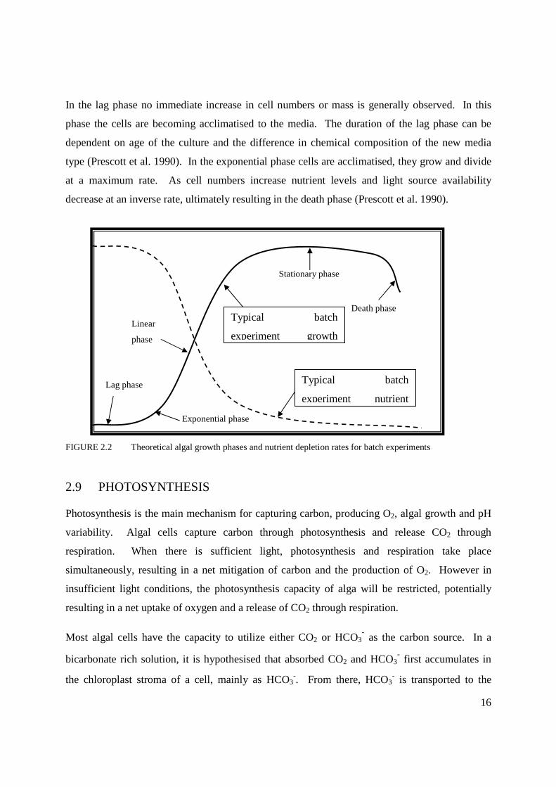
2.8 GROWTH PHASES

Figure 1.2 represents the theoretical algal growth curve and the nutrient depletion curve for a

batch experiment. There are five distinct growth phases that alga can transition through in this

type of experiment. These are the lag phase, exponential phase, linear phase, stationary phase

and the death phase (Mata et al. 2010).

16

In the lag phase no immediate increase in cell numbers or mass is generally observed. In this

phase the cells are becoming acclimatised to the media. The duration of the lag phase can be

dependent on age of the culture and the difference in chemical composition of the new media

type (Prescott et al. 1990). In the exponential phase cells are acclimatised, they grow and divide

at a maximum rate. As cell numbers increase nutrient levels and light source availability

decrease at an inverse rate, ultimately resulting in the death phase (Prescott et al. 1990).

FIGURE 2.2 Theoretical algal growth phases and nutrient depletion rates for batch experiments

2.9 PHOTOSYNTHESIS

Photosynthesis is the main mechanism for capturing carbon, producing O2, algal growth and pH

variability. Algal cells capture carbon through photosynthesis and release CO2 through

respiration. When there is sufficient light, photosynthesis and respiration take place

simultaneously, resulting in a net mitigation of carbon and the production of O2. However in

insufficient light conditions, the photosynthesis capacity of alga will be restricted, potentially

resulting in a net uptake of oxygen and a release of CO2 through respiration.

Most algal cells have the capacity to utilize either CO2 or HCO3- as the carbon source. In a

bicarbonate rich solution, it is hypothesised that absorbed CO2 and HCO3- first accumulates in

the chloroplast stroma of a cell, mainly as HCO3-. From there, HCO3

- is transported to the

Stationary phase

Lag phase

Exponential phase

Linear

phase

Death phase Typical batch

experiment growth

Typical batch

experiment nutrient

17

thylakoid lumen and converted into CO2 in the acid lumen. The concentration of CO2 is then

diffused through pyrenoid tubules in the thaylakoid membrane to the pyreniod matrix, where it is

fixed by Rubisco (Chi et al. 2011).

According to equilibrium:

H2O + CO2 « » H+ + HCO3-

water carbon dioxide

hydrogen ion

bicarbonate ion

Thus, H+ is consumed during the conversion of HCO3- to CO2, and this CO2 is fixed by Rubisco

during photosynthesis. Therefore, when HCO3- is used as the carbon source for photosynthesis,

a build up of OH- remains in the cell, this build up is neutralised by the uptake of H+ from the

extracellular environment. Consequently, the uptake of H+, results in an increase in the pH level

of a solution (Chi et al. 2011). Therefore photosynthesis using a bicarbonate source leads to

increases in pH of a medium.

2.10 ALGAL HARVESTING

There is still no universal method for harvesting algae. The development of an appropriate and

economical process is an ongoing active area of research (Mata et al. 2010). Common methods

adopted today include sedimentation, centrifugation, filtration and ultra-filtration. Flocculation

can be used to facilitate harvesting methods. This process aggregates microalgae, increasing

effective particle size, therefore making the collection of cells a simpler process (Mata et al.

2010).

2.11 CHAPTER SUMMARY

This chapter reviewed the literature relevant to microalgae biofuel and the potential benefits of

its application. A review was made of the properties of CSG water and its possible utilization.

The topics of decentralisation, fuel security, culturing techniques and photosynthesis in a

bicarbonate medium were discussed.

18

CHAPTER 3 METHODOLOGY

The assessment of growth, lipid production, carbon sequestration and nutrient depletion rates of

microalgae strands Dunaliella tertiolecta in CSG water, and Chlorella vulgaris in an MBL

medium, consisted of the following steps.

1. Culturing of microalgae

2. Collection and preparation of medium

3. Determination of water characteristics and nutrient/carbon addition

4. Online monitoring of pH, DO and temperature in the bio-reactor

5. Sample collection for carbon, nitrogen, phosphorous, spectroscopy and suspended

solids, as well as measurement of medium volumes within the bioreactor

6. Harvesting and freeze drying of algae

7. Lipid extraction and analysis

8. Collation and assessment of data

3.1 CULTURING OF MICROALGAE

3.1.1 ALGAL STRAND DUNALIELLA TERTIOLECTA

A sample (20mL) of microalgae strand Dunaliella tertiolecta was ordered from the CSIRO’s

Australian National Algae Culture Collection, located in Hobart, Tasmania. The strand was first

pre-cultured in 250ml flasks in an F/2 medium (1mL/L) (Refer to section 3.3.3). Culturing was

initially conducted in two different salinities, with NaCl levels of 3.5g/L (CSG water equivalent),

and 35g/L (Seawater equivalent).

3.1.2 ALGAL STRAND CHOLERA VULGARIS

A pre-existing culture of Cholera vulgarise was acquired from the USQ (FoES) Environmental

Engineering laboratory. The algal stand was re-cultured in 250ml flasks using a prepared MBL

media.

19

3.2 WATER COLLECTION AND PREPERATION

3.2.1 CSG WATER

The CSG water was obtained from the National Centre for Engineering in Agriculture (NCEA),

located on the USQ Toowoomba campus. The water was initially acquired by the NCEA from a

CSG exploration company. Due to confidentiality restrictions, the original source of the CSG

water cannot be identified.

The collected CSG water was filtered using 0.45µm filter paper, with the aid of a vacuum pump

system. The water was then stored between 20°C to 25°C in the USQ (FoES) Environmental

Engineering laboratory, before being utilized in the bioreactor experiments.

3.2.2 MBL MEDIA

The MBL media was prepared in the USQ (FoES) Environmental Engineering laboratory.

Details of the components and preparation method of the solution are provided in section 3.3.2.

3.3 WATER CHARICTERISTICS AND NUTRIENT/BICARBONATE

ADDITION

3.3.1 CSG WATER

The obtained CSG water was tested for total carbon (TC) and total nitrogen (TN), using a Total

Organic Carbon/Total Nitrogen Analyzer (TOC-VCPH/CPN). Ion composition (F, Cl, NO2,

NO3 and PO4) was assessed, using the Ion Chromatography system (IC, Dionex ICS 2000).

Results are shown in Table 3.1. Research by Kinnon et al (2010) (Section 1.5) provides a more

detailed listing of CSG water compositions, for various sample sites and depths in the Surat

basin.

20

TABLE 3.1 Composition of CSG Water sample

Elements Concentration (mg/L)

Total Organic Carbon/Total Nitrogen Analyzer (TOC-VCPH/CPN).

Total Carbon (TC) 23.5 C mg/L

Total Nitrogen (TN) 0.3 N mg/L

Ion Chromatography system (IC, Dionex ICS 2000)

Fluorine (F) 6.5 F mg/L

Chlorine (Cl) 805.5 mg/L

Nitrite (NO 2) 0.0 mg/L

Nitrate (NO3) 0.0 mg/L

Phosphate (PO4) 0.0mg/L

3.3.2 CARBON ADDITION TO CSG WATER

Based on the findings by (Kinnon et al. 2010), concentrations of bicarbonate (expressed as

calcium carbonate (CaCO3)) in CSG water, were shown to vary between 300 mg/L to 2,860

mg/L, with an average mean concentration of 901.5 mg/L (216 C mg/L). The low levels of

carbon found in the current CSG water samples (24 C mg/L), suggest that the water has

previously been treated. To emulate real life CSG water conditions, the bicarbonate level in the

water was increased to the mean concentration level (216 C mg/L), through the addition of

sodium bicarbonate (NaHCO3).

3.3.3 F/2 CONCENTRATE

An F/2 concentration (Algaboost), was ordered from AusAqua Pty Ltd. The F/2 concentrate was

used to provide key nutrients such as phosphate and nitrogen and other vital vitamins, to

facilitate the growth of Dunaliella tertiolecta in a CSG medium. The composition of F/2 was not

supplied by the manufacturer, therefore initial testing was undertaken to assess nutrient

quantities. Adopting an initial dosage rate of 1ml F/2 to 1 L CSG water, the following nutrient

concentrations results were obtained (Table 3.2).

21

TABLE 3.2 Composition of CSG Water sample (plus 1mg/L of F2 concentrate)

Elements Concentration (mg/L)

Total Organic Carbon/Total Nitrogen Analyzer (TOC-VCPH/CPN).

Total Carbon (TC) 26.5 C mg/L

Total Nitrogen (TN) 13.1 N mg/L

Ion Chromatography system (IC, Dionex ICS 2000)

Fluorine (F) 6.2 F mg/L

Chlorine (Cl) 802.5 mg/L

Nitrite (NO 2) 0.0 mg/L

Nitrate (NO3) 93.5 NO3- mg/L (21.0 N mg/L)

Phosphate (PO4) 5.5 PO4 mg/L (1.7 P mg/L)

Results show recorded nitrogen levels from the two machines varying between 13.1 mg/L and

21.0 mg/L, and a phosphorous reading of 1.7 mg/L. F/2 media composition does not indicate the

presence of ammonia or organic nitrogen that could have shown increased TN concentration

measured via TOC machine. Assuming an average nitrogen reading of 17 mg/L, this gave a N:P

ratio of approximately 10:1.

For the Dunaliella tertiolecta trials, the F/2 dosing rate was increased to 5ml concentrate per 1 L

of CSG water. The intention of this increased dosage was to avoid phosphate concentrations in

the trial periods dropping below the measuring range capacity of the Ion Chromatography system

(IC, Dionex ICS 2000) indicating the possibility of P limiting the growth of algae. This increase

in dosage resulted in a final C:N:P ratio of 192:85:8.5. Although this adjustment meant that the

ratio of carbon was below theoretically optimal levels, it was predicted that due to the short

period of the Dunaliella tertiolceta trials (5 days), carbon availability would not become an

issue.

22

3.3.4 MBL MEDIA

The MBL media was prepared as shown in Table 3.3 (Nichols 1973).

Stock Solutions Per Litre Distilled/milliQ water

CaCl2.2H2O 36.76g

MgSO4.7H2O 36.97 g

NaHCO3 12.60 g

K 2HPO4 8.71 g

NaNO3 85.01 g

Na2SiO3.9H2O 28.42 g

Na2EDTA 4.36 g

FeCl3.6H2O 3.15 g

Metal Mix

CuSO4.5H2O

ZnSO4.7H2O

CoCl2.6H2O

MnCl 2.4H2O

Na2MoO4.2H2O

0.01 g

0.022 g

0.01 g

0.18 g

0.006 g

Add each component separately to

750 mL, fully dissolved between

additions and then increase volume

to 1 L with distilled water

Vitamin Stock

Cyanocobalamin (Vitamin B12)

Thiamine HCl (Vitamin B1)

Biotin

0.0005 g/L

0.10 g/L

0.0005 g/L

Tris stock 250.00 g/L

TABLE 3.3 Composition of MBL media

3.4 BIO-REACTOR DESIGN

The algae based titrimetric bio-reactor (Figure 3.1 & 3.2) was located in the USQ (FoES)

Environmental Engineering laboratory. The bio-reactor enabled the collection of real time data,

relating to the growth of microalgae strands Dunaliella tertiolecta and Chlorella vulgaris in

23

conducted batch experiments. All batch experiments were carried out in a single reactor tank

with a 4L capacity.

3.4.1 INPUT VARIABLES

The utilization of compressed air and CO2 inputs was subject to the specific parameters of each

experiment, refer to Chapters 4, 5 & 6 for further details. In applicable experiments, compressed

air was supplied continuously into the bio-reactor at a rate of 250ml/min. CO2 input was used in

the experiments with Chlorella vulgaris in MBL media, to provide a carbon source. The timing

and input of CO2 addition was controlled by the Labview program. When utilized, CO2 was

administered continually at a steady rate of 5 ml/min, and in concentrated (60ml/min) 4 second

burst, once every 2 hours.

No CO2 input was provided for the first 2 days of the Chlorella vulgaris experiments. Initial

trials and previous experimental works found the buffer capacity of the solution was poor in the

early stages of these experiments, resulting in unacceptable pH volatility with the addition of

CO2. This poor capacity generally coincided with the lag growth phase, when algal were

generally inactive.

A light source was provided using three florescent tubes (2000 lux each). The tubes were

positioned on three sides of the tank, at a distance of 5 cm away. Light was supplied for 12

hours per day, from 6am to 6pm. A stirrer was also used at a constant rate for mixing purposes.

Figure 3.1 shows the schematic of the bio-reactor.

24

FIGURE 3.1 Schematic diagram of the Bio-reactor

3.4.2 pH MONITORING AND CONTROLLING

An Ionode pH electrode was positioned within the 4 L bio-reactor tank and was connected to a

pH transmitter (TSP Mini Chem), which provides real time pH measurements. Readings from

the pH transmitter were also linked to the integrated laptop. The Labview program logged pH

levels, and allowed for the set-limit of a pH range. The pH level within the tank was controlled

by acid (0.1 N H2SO4) and base (0.1 N NaOH) addition. Acid and base were continuously

pumped around a tube loop network with a peristaltic pump, this enabled a constant pressure to

be kept and allowed accurate dose rates (10ml) to be administered to the tank through a 3-way

solenoid valves.

3.4.3 DO AND TEMPERATURE MONITORING

A dissolved oxygen electrode (YSI) was positioned within the bioreactor, it connected to a

dissolved oxygen meter (TPS 90-D), which provided real time DO and temperature readings.

The DO meter was linked to the integrated laptop, onto which all results were logged.

3 x Light

Source

Air

Reactor Timer

pH DO

Base

Acid

Pump

Stirrer

25

The temperature of the lab was regulated at 25°C using the building’s air-conditioning system.

However results found temperature fluctuations between 19°C and 24°C. Temperature

correction was made to the obtained DO readings to a base level of 20°C.

3.4.4 LABVIEW PACKAGE

The Labview software monitored pH, DO and temperature serial outputs from the pH transmitter

and the DO meter, with high frequency. The 0-1 volt signals from the transmitter and meter

where logged in the integrated laptop with the Labview software, and a combined A/D I/O card

(National Instruments, PCI-6013). All recorded data was saved in Microsoft Excel spreadsheet

format. The user could set experiment parameters on the front panel of the program, with

tolerance set-point limits. Figure 3.2 shows the bio-reactor set up.

FIGURE 3.2 The Bio-reactor setup.

CO2

solenoid

Integrated

laptop

Acid &

Base

CO2 supply

Air supply

DO & Temp

meter

Stirrer

Lighting

pH meter

Timer

Bio-reactor –

including pH,

DO and temp

probes

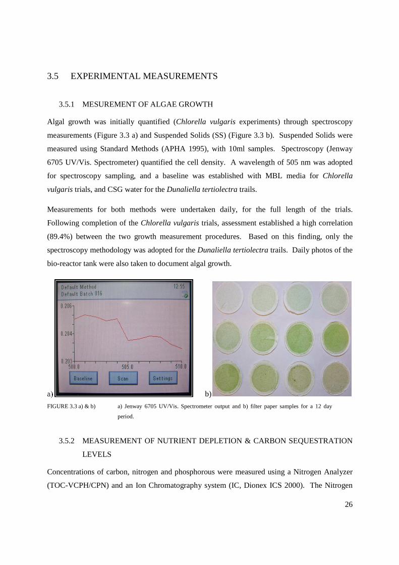
26

3.5 EXPERIMENTAL MEASUREMENTS

3.5.1 MESUREMENT OF ALGAE GROWTH

Algal growth was initially quantified (Chlorella vulgaris experiments) through spectroscopy

measurements (Figure 3.3 a) and Suspended Solids (SS) (Figure 3.3 b). Suspended Solids were

measured using Standard Methods (APHA 1995), with 10ml samples. Spectroscopy (Jenway

6705 UV/Vis. Spectrometer) quantified the cell density. A wavelength of 505 nm was adopted

for spectroscopy sampling, and a baseline was established with MBL media for Chlorella

vulgaris trials, and CSG water for the Dunaliella tertiolectra trails.

Measurements for both methods were undertaken daily, for the full length of the trials.

Following completion of the Chlorella vulgaris trials, assessment established a high correlation

(89.4%) between the two growth measurement procedures. Based on this finding, only the

spectroscopy methodology was adopted for the Dunaliella tertiolectra trails. Daily photos of the

bio-reactor tank were also taken to document algal growth.

a) b)

FIGURE 3.3 a) & b) a) Jenway 6705 UV/Vis. Spectrometer output and b) filter paper samples for a 12 day

period.

3.5.2 MEASUREMENT OF NUTRIENT DEPLETION & CARBON SEQUESTRATION

LEVELS

Concentrations of carbon, nitrogen and phosphorous were measured using a Nitrogen Analyzer

(TOC-VCPH/CPN) and an Ion Chromatography system (IC, Dionex ICS 2000). The Nitrogen

27

Analyzer measured carbon (TOC, IC & TC) and nitrogen (TN) levels, the Chromatography

system was used to measure phosphorous (PO4) and also nitrogen (NO2 & NO3) levels. Daily

samples (15ml Nitrogen Analyzer, 5ml Chromatography system), were taken throughout the trial

periods. Prior to sampling, algae were put into suspension by temporarily accelerating the

rotational speed of the stirrer. Before sampling, the volume of the media was recorded,

concentration adjustment was subsequently made to all results at the data analysis stage (Refer to

section 3.8). Note that only nitrogen levels were assessed in the Chlorella vulgaris trials.

Two daily samples were taken from each analysis for the Dunaliella tertiolecta trials, average

readings were derived from the results. To reduce volume losses in the bioreactor, samples were

diluted with distilled water at a ratio of 1:4 (media:distilled water).

3.5.3 MEASUREMENT OF DO AND pH DATA

The pH and DO probes were calibrated before the commencement of each trial, to maintain

accuracy. Readings from the monitoring equipment were logged at 1 minute intervals, into the

Labview software (Figure 3.4). The continual real-time monitoring allowed the researcher the

capacity to intervene if data monitoring faults or growth behaviour issues arose. The pH, DO

and temperature monitoring components of the bio-reactor are described in Section 3.4.

Logged readings allowed for observational and quantifiable assessment. Documented sudden

drops in pH levels were typically associated with acid or CO2 addition, conversely sudden spikes

in pH represented base addition. Algal growth behaviour was identifiable by steady variations in

pH levels. DO readings allowed for the identification of photosynthesis and respiration

behaviours of the algae. It also allowed for the calculation of oxygen production quantities of the

algae. Refer to section 2.7 for further details regarding algal growth behaviour and its influence

on pH and DO levels.

At the completion of a trial, all data was collated in Excel format. Temperature adjustment was

made to DO readings, to maintain a 20°C base temperature. DO and pH results were then

graphed using the computer program MATLAB. Graphed results allowed for the identification

and adjustment of outliers.

28

FIGURE 3.4 Labview software output logging DO, pH, temperature and acid/base addition in real time.

3.6 MICROALGAE HARVEST

Alga was separated from the water using a two step centrifugation process. Initially algae

underwent centrifugation at 8000rpm for 10 minutes, with a 3 minute cool down period

(Beckman Avanti CentrifugeJ-25 I) (Figure 3.5 a). Excess water was then removed, and the

algae were washed with distilled water, before undergoing a second stage of centrifugation at

4000rpm for 10 minutes (Eppendorf Centrifuge 5810 R) (Figure 3.5 b). Once separation was

complete, the algae pellets were frozen for 24 hours and then freeze dried at -56°C and 30torr

(VirTis 2KBTES-55)(Figure 3.5c). They were then stored at room temperature in a desiccators,

for later lipid measurements. The timing and the growth phase at which the algae were harvested

was specific to each experiment.

Acid

pH

DO

Temperature

Base

29

a) c)

FIGURE 3.5 a), b) & c) a) Beckman Avanti CentrifugeJ-25 I, b) Eppendorf Centrifuge 5810 R and c)

VirTis 2KBTES-55 Freeze Dryer.

3.6.1 MEASUREMENT OF ALGAL DRY WEIGHT

To obtain the algal dry weight, the freeze dry jar was first weighed before algae were added.

After freeze drying the jar with the algae was re-weighed. The dry weight of the algae was equal

to the difference between two measurements, as shown in equation 3.1.

b)

30

3.7 LIPID EXTRACTION AND ANALYSIS

The lipid content of the freeze dried algae was extracted using a modified version of the Folch

method (Folch et al 1957). Modification was required, due to the small sample sizes. The

following steps were taken.

1. Place sample in 5 ml McConkey bottle.

2. Add 1.6 ml of CHCl3 and 0.8 ml of MoOH (ratio 2:1)

3. Parafilm under lid, shake by hand for 20min

4. Transfer to 10 ml centrifuge tube, wash with 1.0 ml of CHCl3

5. Spin at 3000rpm for 10 minutes

6. Transfer upper phase to new centrifuge, use distilled water to transfer

7. Spin again at 3000rpm for 10 minutes

8. Siphon off top layer and discard.

9. Transfer bottom layer to new 5 ml McConkey. Use CHCl3 to mix, use no more than 1.5 ml. Open lid evaporate in hood up to 2 days.

Once all steps are completed, samples are then dried and weighed to determine lipid content.

3.8 DATA ANALYSIS

3.8.1 CARBON AND NUTRIENT UTILIZATION CALCULATIONS

Reductions of the media volume within bio-reactor, resulting from evaporation and sampling,

altered the carbon and nutrient concentrations. To account for this concentration variability,

daily recorded tank volumes, time lapse periods between samples and carbon/nutrient sampling

results, were entered into an excel spreadsheet, for correction.

Correction methodology differentiated between the Chlorella vulgaris and Dunaliella tertiolecta

trials. In the Chlorella vulgaris trials, MBL media was initially used to top up the tank volume,

consequently this nutrient addition had to be accounted for. In the Dunaliella tertiolecta trials,

only distilled water was used for toping up, therefore no additional nutrients were added to the

media after commencement of the trial.

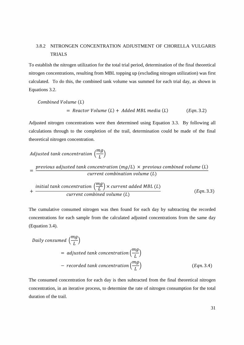
31

3.8.2 NITRONGEN CONCENTRATION ADJUSTMENT OF CHORELLA VULGARIS

TRIALS

To establish the nitrogen utilization for the total trial period, determination of the final theoretical

nitrogen concentrations, resulting from MBL topping up (excluding nitrogen utilization) was first

calculated. To do this, the combined tank volume was summed for each trial day, as shown in

Equations 3.2.

�� . 3.2�

Adjusted nitrogen concentrations were then determined using Equation 3.3. By following all

calculations through to the completion of the trail, determination could be made of the final

theoretical nitrogen concentration.

�� !�� "�#� $

� %��&�� !�� #/�� ( %��&�� &�� &��

��!�� "�#

� $ ( �� &�� . 3.3�

The cumulative consumed nitrogen was then found for each day by subtracting the recorded

concentrations for each sample from the calculated adjusted concentrations from the same day

(Equation 3.4).

)��*�� "�#� $

� �� !�� "�#� $

+ ��!�� "�#� $ ��. 3.4�

The consumed concentration for each day is then subtracted from the final theoretical nitrogen

concentration, in an iterative process, to determine the rate of nitrogen consumption for the total

duration of the trail.

32

3.8.3 CONCENTRATION ADJUSTMENT FOR DUNALIELLA TERTIOLECTA

TRIALS

Unconsumed levels were determined by first multiplying the recorded tank volumes (L) for each

day, by the initial sample reading (mg/L), this gave the initial nutrient/carbon values (mg).

These values were then divided by current water levels to determine unconsumed levels

(Equation 3.5).

-�� "�#� $ � �� #�

��.��&�� . 3.5�

Daily consumed/lost levels of nutrients and carbon was then determined by subtracting sample

readings from derived unconsumed nutrient values. The consumed/lost concentration for each

day is then subtracted from the unconsumed concentration in an iterative process. This

adjustment method was used for nutrients, carbon and growth measurements.

3.8.4 SPECIFIC GROWTH RATE CALCULATIONS

The specific growth rate was calculated for nutrient depletion and oxygen release. Nutrient

depletion was found by dividing the slope of the nutrient change over a time period by the slope

of the optical density reading over the same time period (Eqn. 3.7). Oxygen production during

the day time, was equal to area under DO graphs for a 24 hour period divided by the light period

(hr) and multiplied by the wastewater volume in the bioreactor (Eqn. 3.8). The DO area under

the graph was established by setting night DO levels as the baseline.

0%��1��#��.�2��

�0��%� ��

0��%� �%�� *��

��. 3.7�

45*#��%��#��#2�%�� #�

� ��)4#��%2��#2�%�� ( .� ��.��&�� 3.8�

33

3.8.5 DATA MANIPULATION

In the batch experiments, Lab View continually logs all online data into an Excel spreadsheet.

Error readings for DO, pH and temperature were corrected manually through linear

approximations. Due to the large amount of raw data produced, Matlab was utilised for all

graphical presentation purposes. Dissolved oxygen readings were converted to 20°C equivalent

values, through the use of automated lookup tables. Trial time readings were logged in excel, in

the form of text (24 hour period, serial numbers), in hours, minutes and seconds, e.g. 083200

represented 8:32am. For use in Matlab time readings were converted to decimal days. Logged

Excel trial time data was first converted to a dd:hh:mm:ss format to include cumulative day

values, cell values were then converted to decimal day values. For example 3:35pm on Day 5,

was first changed to 05:15:35:00, and then to 5.634722.

A line used to indicate light and dark periods was included into the graphical results. The

illustrative line was developed by inserting another column into the excel results and manually

entering two alternating values corresponding to light and dark periods, i.e. inputting 5 for the

light period and 3 for the dark period.

3.9 RISK MANAGEMENT

Before commencing work within the USQ laboratories, the researcher was required to undergo a

safety induction and complete a Safe Work Procedures form, to assists in identifying potential

safety issues that may arise during the project period. The following safety concerns were

identified.

3.9.1 WORKING WITH HAZARDS CHEMICALS

The project required the use of hazardous chemicals including concentrated acid and base

solutions. To avoid potential harm, PPE including gloves, face marks, eye protection and closed

shoes were worn as required. All diluting of concentrated acid/base solutions will be undertaken

within the venting chamber.

34

3.9.2 DISEASE PREVENTION

When using wastewater, there was a potential of bacterial contamination. To prevent

contamination, gloves were worn when appropriate, and a disinfectant hand wash was used after

any handling of waste products.

3.9.3 DISPOSAL METHOD OF BIOHAZARD MATERIALS

Because the bio-hazardous materials contained vast amounts of microalgae, they could not be

discharged directly down the sink, as there is a high risk of algae growth in the drains causing

clogging. As such when disposing of large amount of algae, it was first autoclaved and then

disposed of.

3.9.4 RISKS BEYOND COMPLETION OF THE PROJECT

Following completion of this project, all waste materials were correctly disposed of, all

chemicals were stored away, and the bioreactor was unplugged, cleaned and put aside until

future use. Therefore no safety risk posed beyond the completion of the project by the materials

used or microalgae growth mediums created.

3.10 CHAPTER SUMMARY

This chapter discussed the procedure for collection and preparation of algae and media, methods

for determining CSG water characteristics, as well as adopted methods for calculating required

levels of nutrient and bicarbonate addition. The bio-reactor set up was described and an

overview was provided of the monitoring and logging processes for DO, pH and temperature

readings. Adopted methodology for measurement of algal growth and nutrient depletion was

examined. Methods for algal harvesting, freeze drying and lipid extraction were reviewed.

35

CHAPTER 4 GROWTH CHARICTERISTICS OF

MICROALGAE CHLORELLA VULGARIS

GROWN IN MBL MEDIA AND THE EFFECTS

OF CO2 INPUT.

This chapter presents the results and discussions on the growth behaviour and nutrient removal

of Chlorella vulgaris in MBL media, using batch experiments. The discussions further extend to

interpret the observations on real-time monitoring using the dissolved oxygen and pH probes

during the growth period.

4.1 BATCH EXPERIMENTS

Two batch experiments were performed using MBL media. Trials were differentiated by the

inclusion of a CO2 gas input in Experiment 1. The purpose of the experiments was twofold, to

determine the effects of CO2 input on algal growth, and to assess the effectiveness of on-line

measurement systems as indicators of the real-time algal growth.

4.1.1 EXPERIMENT 1 (MBL MEDIA – CO2 ADDITION)

Experiment 1 was intended as an assessment of the bioreactors capacity to facilitate and measure

algal growth. At the commencement of the trial, 2 litres of MBL media was inoculated with 250

ml of Chlorella vulgaris culture (6.95mg of biomass). Monitoring of growth and nutrient

removal was conducted for the entire length of the trial. In order to mimic the real world

scenario, photo-energy required for the algal growth was provided by means of a light source.

The light source was implemented on a 12 hour on (6am to 6pm)/off cycle.

36

4.1.2 EXPERIMENT 2 (MBL MEDIA – NO CO2 ADDITION)

The only variable changed for Experiments 2 was the removal of CO2 input. It was predicted

that growth and subsequent lipid production and nutrient removal would be reduced with the

absence of CO2 feed. This experiment was essentially conducted to check for a placebo effect.

4.2 ALGAL GROWTH

Algal growth was quantified using daily Suspended Solids (SS) and Spectrometer measurements.

Photo documentation was also used to capture the transition of algal growth through the various

phases.

4.2.1 EXPERIMENT 1: GROWTH CHARICTERISTICS

Figure 4.1 shows the recorded growth trends of Chlorella vulgaris in Experiment 1, represented

through optical density and suspended solids measurements. The added trend lines are based on

a 3rd order polynomial. Results suggest a lag phase occurring within the first day of the

experiment. Lag phase normally occurs when an inoculums is transferred from its ideal media

into an alternate media with different compositions. When introduced, algae first take some time

to get acclimatized in a new environment. In this study however, the lag period was reduced due

to there being no change in media type from culturing to inoculation, as such transfer shock was

minimal.

The exponential growth period appears to take place between days 1 and 3, with a linear growth

phase from day 3 to 7, and a stationary phase extending from day 7 through to the completion of

the trial. In order to get the maximum lipid extraction, the trial was terminated just before the

expected death phase.

Log records showed that approximately 100ml of media in the bioreactor was lost per day as a

result of evaporation and sampling. For the first two weeks of the trial, MBL media was used to

replace any losses within the bioreactor. The continual addition of a nutrient rich media was

adopted with the intention of prolonging the stationary growth phase. It was thought that by

prolonging this steady phase consistent algae growth and nutrient depletion measurements could

37

be achieved. Obtained results generally confirmed this theory. From the start of the third week,

the MBL media was substituted with distilled water for topping up.

FIGURE 4.1 Experiment 1 – Algal growth in MBL media with CO2 addition measured with Optical Density (�)

at 505 nm and Suspended Solids (�)

Figures 4.2 show the relationships between suspended solids and optical density measurements

for Experiment 1. This relationship can be expressed as shown in Equation 4.1. The result

suggests a moderate correlation (68.8%) between the two algal growth measurement procedures.

Suspended Solids = 0.06367 Optical Density + 0.0098 (R2 = 68.8%) (Eqn. 4.1)

FIGURE 4.2 Experiment 1 - Relationship between Suspended Solids and Optical Density at 505nm.


Figure 4.3 shows the recorded growth characteristics of Chlorella vulgaris without CO2 input.

The trend line was again derived using a 3rd order polynomial. The data suggests a lag phase

occurring within day 1 of the experiment, with an exponential growth period between days 1 and

3. The linear growth trend looks to have extended from days 3 through to 8, followed by a brief

0.00

0.10

0.20

0.30

0.40

0

0.1

0.2

0.3

0.4

0.5

0 5 10 15 20

Su

spe

nd

ed

So

lids

[g/L

]

Op

tica

l De

nsi

ty

Time Elaspe [d]

0.00

0.10

0.20

0.30

0.40

0 0.05 0.1 0.15 0.2 0.25 0.3 0.35 0.4 0.45Susp

en

de

d S

olid

s

(g/L

)

Optical Density

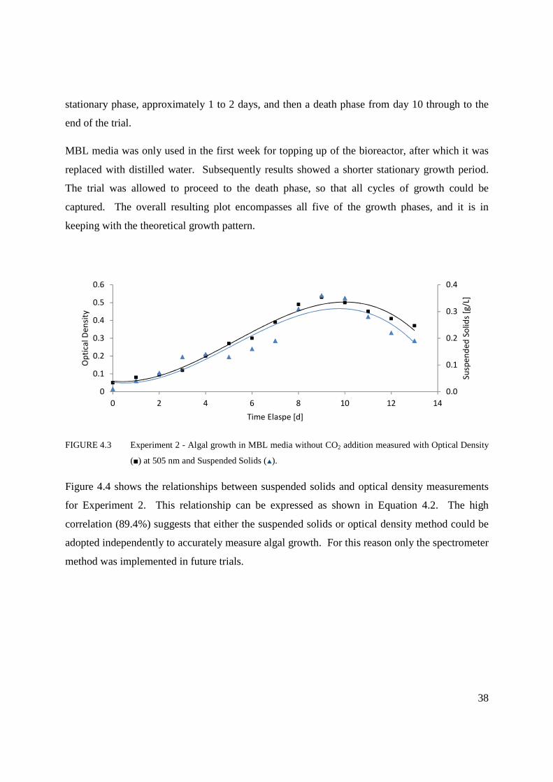
38

stationary phase, approximately 1 to 2 days, and then a death phase from day 10 through to the

end of the trial.

MBL media was only used in the first week for topping up of the bioreactor, after which it was

replaced with distilled water. Subsequently results showed a shorter stationary growth period.

The trial was allowed to proceed to the death phase, so that all cycles of growth could be

captured. The overall resulting plot encompasses all five of the growth phases, and it is in

keeping with the theoretical growth pattern.

FIGURE 4.3 Experiment 2 - Algal growth in MBL media without CO2 addition measured with Optical Density

(�) at 505 nm and Suspended Solids (�).

Figure 4.4 shows the relationships between suspended solids and optical density measurements

for Experiment 2. This relationship can be expressed as shown in Equation 4.2. The high

correlation (89.4%) suggests that either the suspended solids or optical density method could be

adopted independently to accurately measure algal growth. For this reason only the spectrometer

method was implemented in future trials.

0.0

0.1

0.2

0.3

0.4

0

0.1

0.2

0.3

0.4

0.5

0.6

0 2 4 6 8 10 12 14

Su

spe

nd

ed

So

lids

[g/L

]

Op

tica

l De

nsi

ty

Time Elaspe [d]

39

Suspended Solids = 0.06058 Optical Density + 0.0017 (R2 = 89.4%) (Eqn. 4.2)

FIGURE 4.4 Experiment 2 - Relationship between Suspended Solids and Optical Density at 505NM.

Photographic documentation of the Chlorella vulgaris growth in the bioreactor, for Experiment 2

is shown in Figure 4.5. A photo was taken for each of the 14 days of the experiment, recordings

show the algae’s transition through all of the growth phases, approximate labelling of each phase

is provided.

|‹- Day 1 (Lag)- -›|‹- - -- - - - Day 1-3 (Exponential) - - -›|‹- - - - - - -- - - - - - - - - - - - Day 4 -8 (Linear) - - - - - - - - - - - - - - - - - - - - - - -›|

|‹- - - Linear - - -›|‹- - - - Day 9 -10 (Stationary)- - - - -›|‹- - - - - - - - - - - - - - - - - - - - - Day 10 -14 (Death) - - - - - - - - - -- - - - - - - - - - ›|

FIGURE 4.5 Daily photos of algae growth in the Bioreactor for Experiment 2, documenting all 5 stages of growth.

0

0.1

0.2

0.3

0.4

0 0.1 0.2 0.3 0.4 0.5 0.6

Susp

en

de

d S

olid

s

(g/L

)

Optical Density

40

4.2.3 ALGAL GROWTH SUMMARY

A comparison of the growth characteristics between the two trials is shown in Figure 4.6. As

would be expected, the trial with CO2 input experiences faster initial growth. Interestingly

however, the non-CO2 input experiment recorded the highest Optical Density and Suspended

Solids readings. For oil production purposes, emphasis would be placed on increasing biomass

to high concentrations within the shorts period of time. As such, current results suggest merit in

CO2 gas addition.

There is significant evidence in research literature to show that CO2 is a key factor in facilitating

algae growth (Watanabe 2005, Brune et al. 2009, Mata et al. 2010). A possible explanation for

the high growth recorded in the non-CO2 input experiment could be that, the algae is extracting

enough CO2 from the atmosphere for growth requirements. The shallow depth, minimal media

volume and large exposed surface area of the bioreactor would have assisted with atmospheric

CO2 extraction.

Alternately the concentration of CO2 in the media may have been too high, inhibiting growth.

Tang el al. (2010) found that algal growth was highly sensitive to the concentration levels of

CO2, with inadequate or excessive CO2 input resulting in poor growth. Further testing with a

focus on CO2 input volumes would be required to determine the cause of the obtained results.

FIGURE 4.6 Experiment 1 & 2 – Comparison of algal growth in MBL media with and without CO2

addition measured with Optical Density (Experiment 1 = �, Experiment 2 = �) at 505 nm and

Suspended Solids (Experiment 1 = �, Experiment 2 = �)

0.0

0.1

0.2

0.3

0.4

0

0.1

0.2

0.3

0.4

0.5

0.6

0 5 10 15 20 25

Su

spe

nd

ed

So

lids

[g/L

]

Op

tica

l De

nsi

ty

Time Elaspe [d]

41

4.3 pH VARIATION

The pH level within the bioreactor was recorded in real-time, measurements were logged once

per minute. pH levels are influenced predominantly by two main factors, the input of CO2, and

light source availability. Addition of CO2 acidifies the medium reducing the pH value

(Watanabe 2005). This factor was only applicable to Experiment 1. Light source availability

within the reactor determines the growth state of the algae. During light periods, algae extracts

CO2 for photosynthesis, pH levels will rise when the rate of inorganic carbon uptake by

microalgae exceeds the rate of CO2 supply (Harrison & Berges 2005).

4.3.1 EXPERIMENT 1: pH VARIATION

Figure 4.5 shows the measured pH fluctuations of Experiment 1. The CO2 was supplied in two

forms; continuously at a rate of 5ml/min, and in periodic bursts at a rate of 60ml/min, injected

once every 2hrs for 4 seconds. The periodic CO2 input only occurred during the light period i.e.

between 6am and 6pm, and was observable by sharp drops in pH every 2 hours.

Overall, the results show volatile readings for the first 2 days, coinciding with the indentified lag

and exponential phases. No CO2 was added during the expected lag and exponential phases,

previous batch experiments conducted in the USQ lab found that the media had insufficient

buffering capacity to accommodate the periodic CO2 addition during these initial stages (Pufelski

2010).

From days 2 to 5, higher stable readings were observed. This time period, relates to the

identified linear growth phase. From day 5 onwards pH levels reduced whilst remaining stable,

they then increased gradually for the remainder of the experiment. The added red line indicates

light and dark periods of the experiment, peaks (light) and troughs (dark).

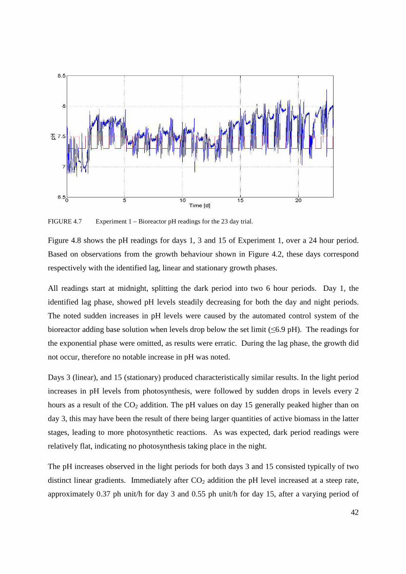
42

FIGURE 4.7 Experiment 1 – Bioreactor pH readings for the 23 day trial.

Figure 4.8 shows the pH readings for days 1, 3 and 15 of Experiment 1, over a 24 hour period.

Based on observations from the growth behaviour shown in Figure 4.2, these days correspond

respectively with the identified lag, linear and stationary growth phases.

All readings start at midnight, splitting the dark period into two 6 hour periods. Day 1, the

identified lag phase, showed pH levels steadily decreasing for both the day and night periods.

The noted sudden increases in pH levels were caused by the automated control system of the

bioreactor adding base solution when levels drop below the set limit (≤6.9 pH). The readings for

the exponential phase were omitted, as results were erratic. During the lag phase, the growth did

not occur, therefore no notable increase in pH was noted.

Days 3 (linear), and 15 (stationary) produced characteristically similar results. In the light period

increases in pH levels from photosynthesis, were followed by sudden drops in levels every 2

hours as a result of the CO2 addition. The pH values on day 15 generally peaked higher than on

day 3, this may have been the result of there being larger quantities of active biomass in the latter

stages, leading to more photosynthetic reactions. As was expected, dark period readings were

relatively flat, indicating no photosynthesis taking place in the night.

The pH increases observed in the light periods for both days 3 and 15 consisted typically of two

distinct linear gradients. Immediately after CO2 addition the pH level increased at a steep rate,

approximately 0.37 ph unit/h for day 3 and 0.55 ph unit/h for day 15, after a varying period of

43

time this rate reduced to approximately 0.17 ph unit/h and 0.34 ph unit/h for days 3 and 15

respectively. This second gradient is more apparent in the day 15 readings. The steepness of the

slope within the two hour period represents different rates of growth, with faster growth initially

upon the addition of carbon dioxide, followed by relatively sluggish growth after a certain time.

FIGURE 4.8 Experiment 1 – Bioreactor pH readings over a 24 hr period for Day 1 (―), Day 3 (―) and

Day 15 (―).


The pH levels for Experiment 2 are presented in Figure 4.9, results show large fluctuation over

the first 2 days, which again coincides with the identified lag and exponential growth phases.

After day 2, the average pH level stabilises and gradually increases until day 5 before declining

for the remainder of the trial. From day 10, the identified commencement of the death phase,

there is a noticeable deterioration in the pH pattern.

The red line shows dark (trough) and light (peak) periods. It is observed that a steady rise in pH

readings occurs during the light periods followed by a steady decline in the dark periods,

generally resulting in a peak pH value at the end of each light period.

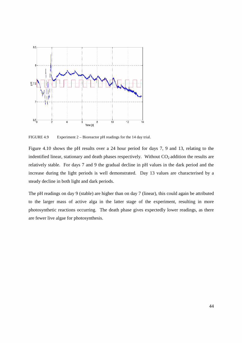
44


Figure 4.10 shows the pH results over a 24 hour period for days 7, 9 and 13, relating to the

indentified linear, stationary and death phases respectively. Without CO2 addition the results are

relatively stable. For days 7 and 9 the gradual decline in pH values in the dark period and the

increase during the light periods is well demonstrated. Day 13 values are characterised by a

steady decline in both light and dark periods.

The pH readings on day 9 (stable) are higher than on day 7 (linear), this could again be attributed

to the larger mass of active alga in the latter stage of the experiment, resulting in more

photosynthetic reactions occurring. The death phase gives expectedly lower readings, as there

are fewer live algae for photosynthesis.

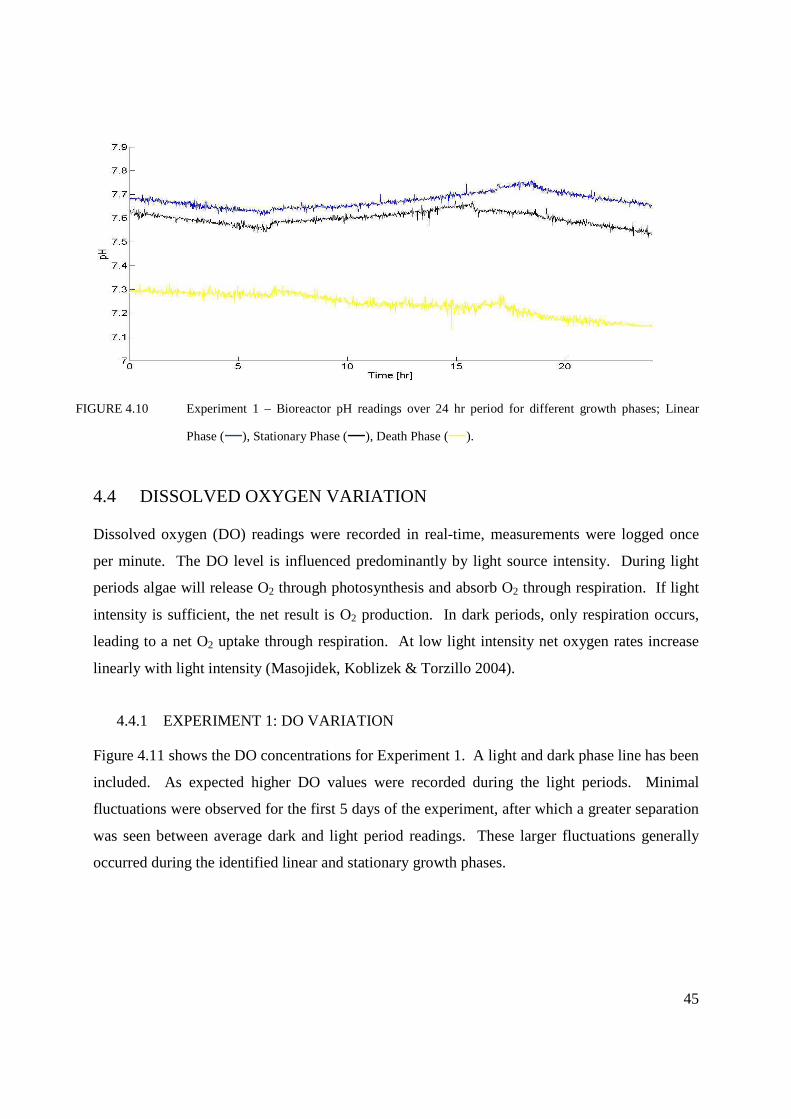
45

FIGURE 4.10 Experiment 1 – Bioreactor pH readings over 24 hr period for different growth phases; Linear

Phase (―), Stationary Phase (―), Death Phase (―).

4.4 DISSOLVED OXYGEN VARIATION

Dissolved oxygen (DO) readings were recorded in real-time, measurements were logged once

per minute. The DO level is influenced predominantly by light source intensity. During light

periods algae will release O2 through photosynthesis and absorb O2 through respiration. If light

intensity is sufficient, the net result is O2 production. In dark periods, only respiration occurs,

leading to a net O2 uptake through respiration. At low light intensity net oxygen rates increase

linearly with light intensity (Masojidek, Koblizek & Torzillo 2004).

4.4.1 EXPERIMENT 1: DO VARIATION

Figure 4.11 shows the DO concentrations for Experiment 1. A light and dark phase line has been

included. As expected higher DO values were recorded during the light periods. Minimal

fluctuations were observed for the first 5 days of the experiment, after which a greater separation

was seen between average dark and light period readings. These larger fluctuations generally

occurred during the identified linear and stationary growth phases.

46

FIGURE 4.11 Experiment 1 – Bioreactor DO readings for the 23 day trial.

Figure 4.12 compares average DO readings during the light period with average DO readings in

the dark period for Experiment 1. The relative difference between these two sets of values

provides the net oxygen produced during each of the light periods. This level of DO production

is indicated with the dashed trend line, which is derived from a 3rd order polynomial. The

saturation value of DO at 20°C is 9.17 mg/L, this is also indicated on the graph, as is the

measured optical density readings for this trial.

The highest recorded DO production reading was 4.6 mg /L, on day 18. Dissolved oxygen

production levels generally increased until the end of day 5 (linear), and remained steady for the

remainder of the trial. This increase in DO production is likely the result of a growing volume of

active biomass during the lag, exponential and linear phases.

47

FIGURE 4.12 Experiment 1 –Average maximum DO readings during the light period (�), average

minimum DO readings during the dark period (�), net oxygen produced during the light

period (Χ) and optical density reading (―).

Figure 4.13 shows the estimate oxygen production quantities in the light periods, for each day of

Experiment 1. Quantities were derived using equation 3.8. Results show a peak oxygen

production of 2.09 mg, produced on day 18.

FIGURE 4.13 Experiment 1 – Daily oxygen quantities produced during the light period

0

0.05

0.1

0.15

0.2

0.25

0.3

0.35

0.4

0.45

0

1

2

3

4

5

6

7

8

9

10

0 5 10 15 20

Op

tica

l De

nsi

ty

Dis

solv

ed

Oxy

ge

n A

dju

ste

d f

or

20

De

gre

es

Ce

lsiu

s [m

g/L

]

Time Elaspe [d]

0

0.5

1

1.5

2

2.5

1 2 3 4 5 6 7 8 9 10 11 12 13 14 15 16 17 18 19 20 21 22 23

Pro

du

ced

Oxy

ge

n (

mg

)

Trial day

9.17mg DO/L

48


Figure 4.14 shows the DO dynamics for Experiment 2, a line indicating light and dark periods

has been included. The results show volatile DO readings extending from the start of the trial

until day 6, after which stabilisation occurs. The overall pattern generally reflects the observed

growth behaviour (Figure 4.3) with an increase in average levels until day 9 followed by a clear

decline in readings for the identified death phase.


Figure 4.15 shows the average light and dark period readings for Experiment 1, also included is

the relative DO production during the light period. Obtained results generally show constant

levels of DO production from the start of the trail until day 10, after which the difference begins

to reduce to zero. Higher average dark and light period readings are achieved in the identified

linear and stationary phases. A maximum DO reading of 4.03 mg /L was recorded on day 3.

49

FIGURE 4.15 Experiment 2 –Average maximum DO readings during the light period (�), average

minimum DO readings during the dark period (�), net oxygen produced during the light

period (Χ) and optical density reading (―).





4.5 NUTRIENT REMOVAL

Nutrient depletion was assessed for Experiment 1, by measuring daily total nitrogen levels in the

bioreactor. Results are shown in Figure 4.17, also included is the optical density readings for

algal growth. The graph captures the relationship between nutrient removal and algae growth,

0

0.1

0.2

0.3

0.4

0.5

0.6

0

2

4

6

8

10

12

14

0 2 4 6 8 10 12 14

Op

tica

l De

nsi

ty

Dis

solv

ed

Oxy

ge

n A

dju

ste

d f

or

20

De

gre

es

Ce

lsiu

s [m

g/L

]

Time Elaspe [d]

0

0.5

1

1.5

2

1 2 3 4 5 6 7 8 9 10 11 12 13 14

Pro

du

ced

Oxy

ge

n (

mg

)

Trial Day

9.17mg DO/L

50

results generally reflect the theoretical relationship as described in section 2.8. As MBL media

was used in the first two weeks for topping up the bioreactor, adjustment has been made to the

recorded nutrient values.

FIGURE 4.17 Experiment 1 – Nutrition removal rate measured through nitrogen depletion (�), and

algal growth in Optical Density (�).

Figure 4.18 shows the nitrogen removal rate 1.167 mg TN/L/d for the first 9 days of the trials.

The corresponding suspended solids rate for this period was 21.0 mg SS/L/d, giving a specific

nutrient removal rate of 0.056mg TN/SS.

FIGURE 4.18 Experiment 1 – Nutrition removal rate measured through nitrogen depletion (�), and

algal growth in Suspended Solids (�).

0

5

10

15

20

25

30

0

0.1

0.2

0.3

0.4

0.5

0 5 10 15 20

To

tal N

itro

ge

n [

mg

/L]

Op

tica

l D

en

sity

Time Elaspe [d]

Slope = 0.021 g SS/L/d

R² = 0.7637

Slope = -1.167 mg TN/L/d

R² = 0.8059

0

5

10

15

20

25

30

0.00

0.10

0.20

0.30

0 2 4 6 8 10

To

tal N

itro

ge

n [

mg

/L]

Susp

en

de

d

Solid

s [g

/L]

Time Elaspe [d]

51

4.6 ALGAE DRY MASS AND LIPID CONTENT

Algal dry mass quantities were, 0.45 g and 0.43 g for experiments 1 and 2 respectively. Results

suggest no distinct benefit in either process for total algal production. Lipid extraction processes

were not undertaken.

4.7 ENCOUNTED PROCEDURAL ISSUES

4.7.1 pH VOLATILITY

Initially it was intended that no pH buffer (Tris) would be added to the media, so as not to inhibit

the pH sensitivity of the solution. However shortly after commencing each of the two trials, pH

fluctuations were observed regularly exceeding the set pH limits (pH 7.5 ± 0.6), resulting in

excessive acid and base addition by the bioreactor automotive system. To address this issue, a

small amount of Tris (125mg/L) was added to the media. The limited Tris addition meant that

future pH movements were still observable and were generally within the set limits.

4.7.2 ALGAL SETTLEMENT AND CLUMPING

Early in the trial it was found that the algae was settling at the base of the tank. To address this,

the speed of the stirrer was gradually increased over a several day period. Care was taken in this

process as there was concern that if the stirring speed was too high it would result in algae death

through shearing.

It was also found that algae would clump onto the DO (Figure 4.19) and pH probes, resulting in

inaccurate readings. This was particularly problematic for the DO reading, as it would reduce

recorded values by between 2 to 4ppm. The alga was removed by gently tapping the probes.

Clumping was reduced by placing the probes within the areas of high turbulence created by the

stirrer.

52

FIGURE 4.19 Algal clumping on the DO probe

4.8 CONCLUSIONS

Research has provided insight into the growth characteristics of microalgae Chlorella vulgaris in

a MBL medium. The algae grew well in both Experiments 1 and 2, with suggested benefit in

CO2 addition to promote rapid algal growth. An acceptable correlation was found between the

suspended solid and spectrometer readings, suggesting that future trials could be measured using

only the spectrometer procedure. Furthermore, assessments were made of the pH and DO

variability, algal dry mass quantities and nitrogen depletion rates.

53

CHAPTER 5 GROWTH CHARICTERISTICS AND LIPID

PRODUCTION OF MICROALGAE

DUNALLIELLA TERTIOLECTA GROWN IN A

CSG WATER MEDIA AND THE EFFECTS OF

AERATION.

This chapter presents the results and discussions on the growth behaviour, carbon sequestration

and nutrient removal of Dunaliella Tertiolecta in CSG water using batch experiments. The

discussion further extends to evaluate the algal growth facilitation capacity and carbon stripping

properties of aeration. This chapter ends with the interpretation of the real-time monitoring

results of dissolved oxygen and pH probes during the growth period.


Two batch experiments were performed using microalgae Dunaliella Tertiolecta in a CSG water

media. Trials were differentiated by the inclusion of a compressed air input in Experiment 2.

The purpose of this distinction was twofold, to determine the effects of a compressed input on

algal growth, and to test for a carbon stripping effect through aeration.

5.1.1 EXPERIMENT 1 (CSG WATER MEDIA – NON-AERATION)

Experiment 1 was conducted to assess the growth capacity of microalgae Dunaliella Tertiolecta

in a CSG water medium, without aeration. The experiment was intended as a lab scale

assessment, to evaluate the algae’s capacity to be grown in an open pond setting. Monitoring of

growth and nutrient removal was conducted for the entirety of the trial. Photo-energy required

for the algal growth was provided by means of a light source, implemented on a 12 hour on (6am

to 6pm)/off cycle .

54

At the commencement of the trial, 3 litres of filtered CSG water was inoculated with 250 ml of

Dunaliella Tertiolecta culture (6.95mg of biomass) and 5 ml/L of F2 concentrate. Sodium

Bicarbonate (NaHCO3) was added to the media (1344mg/L) to increase the bicarbonate levels to

the average CSG water conditions. The C:N:P ratio was 192:85:8.5. Refer to Section 3.3 for

further details.

5.1.2 EXPERIMENT 2 (CSG WATER MEDIA – AERATION)

The only variable changed for Experiments 2, was the addition of aeration, fed into the reactor at

a rate of 100 ml/min. It was predicted that growth and subsequent lipid production and nutrient

removal would increase with an aeration feed. Furthermore, it was hypothesised that aeration

would significantly reduce bicarbonate levels within the media through stripping of carbon.

Refer to Section 1.7.4 for details of aeration properties.


Dunaliella Tertiolecta culture (7.12 mg of biomass) and 5 ml/L of F2 concentrate. Sodium

Bicarbonate (NaHCO3) was added to the media (1344mg/L) to increase carbon levels to the

average CSG water conditions. The C:N:P ratio was 192:85:8.5. Refer to Section 3.3 for further

details.

5.2 ALGAL GROWTH

Algal growth was quantified using daily Spectrometer measurements. Photos were taken to

document the phase transition of algal growth.


Figure 5.1 shows the recorded growth trends of Dunaliella Tertiolecta in Experiment 1,

represented through optical density measurements. The added trend line is based on a 3rd order

polynomial. Results suggest a lag phase occurring within the first day of the experiment. The

exponential growth period appears to take place between days 1 and 2, with a linear growth

phase within days 2 and 3. The stationary phase was observed within day 4, with a transition to

the death phase from day 4.

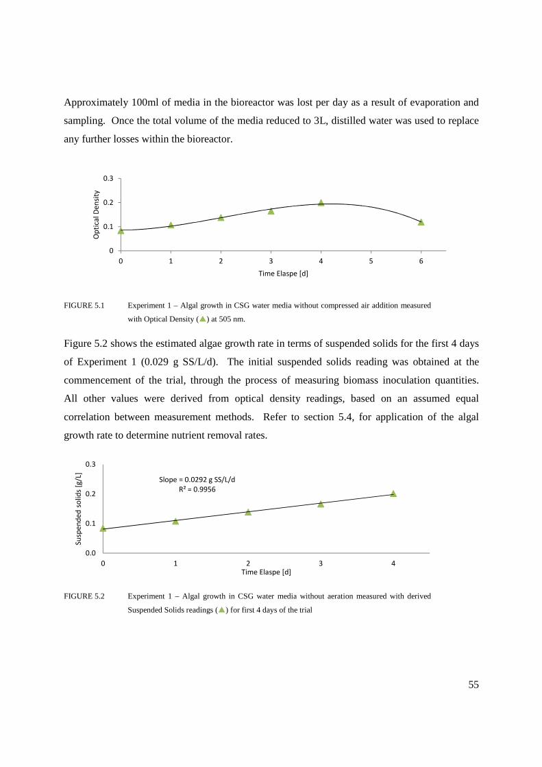
55

Approximately 100ml of media in the bioreactor was lost per day as a result of evaporation and

sampling. Once the total volume of the media reduced to 3L, distilled water was used to replace

any further losses within the bioreactor.

FIGURE 5.1 Experiment 1 – Algal growth in CSG water media without compressed air addition measured

with Optical Density (�) at 505 nm.

Figure 5.2 shows the estimated algae growth rate in terms of suspended solids for the first 4 days

of Experiment 1 (0.029 g SS/L/d). The initial suspended solids reading was obtained at the

commencement of the trial, through the process of measuring biomass inoculation quantities.

All other values were derived from optical density readings, based on an assumed equal

correlation between measurement methods. Refer to section 5.4, for application of the algal

growth rate to determine nutrient removal rates.

FIGURE 5.2 Experiment 1 – Algal growth in CSG water media without aeration measured with derived

Suspended Solids readings (�) for first 4 days of the trial

0

0.1

0.2

0.3

0 1 2 3 4 5 6

Op

tica

l D

en

sity

Time Elaspe [d]


R² = 0.9956

0.0

0.1

0.2

0.3

0 1 2 3 4

Susp

en

de

d s

olid

s [g

/L]

Time Elaspe [d]

56


Figure 5.3 shows the recorded growth characteristics of Dunaliella tertiolecta with aeration. The

trend line was again derived using a 3rd order polynomial. The data suggests a possible

exponential growth phase occurring within day 1 of the experiment, and a linear growth trend on

day 2, followed by a brief stationary phase from days 3 to 4, and then a death phase from day 4

through to the end of the trial. Note that the absence of a documented lag phase, may be due to

the spacing (approx. 24hr) between sampling times, more frequent sampling within the first day

may have revealed a lag period. Distilled water was again used for topping up of the media once

a total volume of 3L was reached.

FIGURE 5.3 Experiment 2 - Algal growth in CSG water media with aeration addition measured with Optical

Density (�) at 505 nm.

Figure 5.4 shows the estimated algae growth rate in terms of suspended solids for the first 4 days

of Experiment 2 (0.030 g SS/L/d). Refer to section 5.4, for application of the algal growth rate to

determine nutrient removal rates.

FIGURE 5.4 Experiment 2 – Algal growth in CSG water media with aeration addition measured with

derived Suspended Solids readings (�) for first 4 days of trial

0

0.1

0.2

0.3

0 1 2 3 4 5 6

Op

tica

l D

en

sity

Time Elaspe [d]


R² = 0.7978

0.0

0.1

0.2

0 1 2 3 4

Susp

en

de

d

solid

s [g

/L]

Time Elaspe [d]

57


A comparison of the growth characteristics between the two trials is shown in Figure 5.5. As

was expected, the trial with aeration input experienced faster initial growth, and recorded the

highest optical density readings (0.229), however difference in growth between trials was not

significant. Furthermore, neither trial achieved high levels of growth, with both trials failing

within 6 days.

FIGURE 5.5 Experiment 1 & 2 – Comparison of algal growth in CSG water media with and without aeration

measured with Optical Density (Experiment 1 = �, Experiment 2 = �) at 505 nm

Due to the poor performance of the trials, assessment was made to identify optimal salinity levels

for Dunaliella tertiolecta growth in a CSG media. Experiments 1 and 2 were then retested using

this identified optimal salinity, refer to Chapter 6 for results.

A comparison of the photographic documentation of Dunaliella tertiolecta growth in the

bioreactor for Experiments 1 and 2 is shown in Figure 5.6. Photos illustrate a relatively poor

growth in both experiments, with a transition to the death phase observable in each experiment

by day 5.

0

0.1

0.2

0.3

0 1 2 3 4 5 6

Op

tica

l De

nsi

ty

Time Elaspe [d]

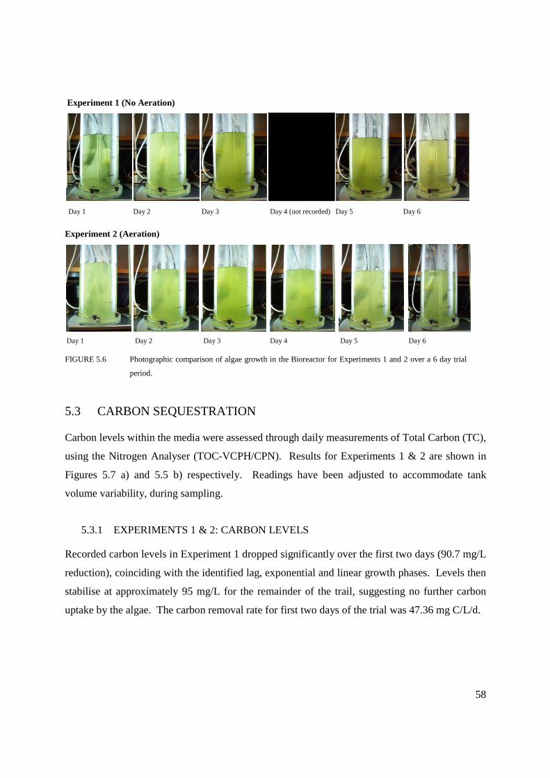
58

Experiment 1 (No Aeration)

Day 1 Day 2 Day 3 Day 4 (not recorded) Day 5 Day 6

Experiment 2 (Aeration)

Day 1 Day 2 Day 3 Day 4 Day 5 Day 6

FIGURE 5.6 Photographic comparison of algae growth in the Bioreactor for Experiments 1 and 2 over a 6 day trial

period.

5.3 CARBON SEQUESTRATION

Carbon levels within the media were assessed through daily measurements of Total Carbon (TC),

using the Nitrogen Analyser (TOC-VCPH/CPN). Results for Experiments 1 & 2 are shown in

Figures 5.7 a) and 5.5 b) respectively. Readings have been adjusted to accommodate tank

volume variability, during sampling.

5.3.1 EXPERIMENTS 1 & 2: CARBON LEVELS

Recorded carbon levels in Experiment 1 dropped significantly over the first two days (90.7 mg/L

reduction), coinciding with the identified lag, exponential and linear growth phases. Levels then

stabilise at approximately 95 mg/L for the remainder of the trail, suggesting no further carbon

uptake by the algae. The carbon removal rate for first two days of the trial was 47.36 mg C/L/d.

59

In Experiment 2, results show a steep decline in carbon levels over the first two days (135.8

mg/L reduction) coinciding with the identified exponential and linear growth phases. The rate of

reduction then changes to a shallower grade for the remainder of the trial, a final reading of

15.66 mg/L was recorded. The carbon removal rate was 74.07 mg C/L/d for first two days of the

trial, and 11.99 mg C/L/d for the remainder of the trial.

a) b)

FIGURE 5.7 a) & b) Total Carbon (TC) readings for (a) Experiment 1 (�) and (b) Experiment 2 (�)

5.3.2 CONTROL TRIAL: CARBON LOSS

A control trial was conducted to identify the rate at which carbon was lost from the CSG media

(within the bio-reactor tank), through processes other than aeration stripping or algal absorption.

The control trial replicated the parameters of Experiment 1, except for the omission of nutrient

addition and algal inoculation. The media was stirred at a constant rate during the trial period,

and no aeration was used.

Results found minimal losses (cumulative loss of 12 mg/L) over the duration of a 6 day trial

(refer to Section 5.3.3), suggesting that the majority of the media’s carbon loss within the bio-

reactor results from aeration or algal absorption for experiments 1 and 2.

5.3.3 CARBON SEQUESTION ASSESSMENT

Figure 5.8 shows the TC rates for Experiments 1, Experiment 2, and the control trial. As nutrient

addition and algal inoculation are the only differing factors between Experiment 1 and the

control trial, the resulting difference in carbon levels between the trials (90.9 mg/L) is likely the

result of carbon sequestration by the algae. Similarly, as there was no significant difference in

0

50

100

150

200

0 1 2 3 4 5

Ca

rbo

n (

mg

/L)

Time elapsed (d)

0

50

100

150

200

0 1 2 3 4 5

Ca

rbo

n (

mg

/L)

Time elapsed (d)

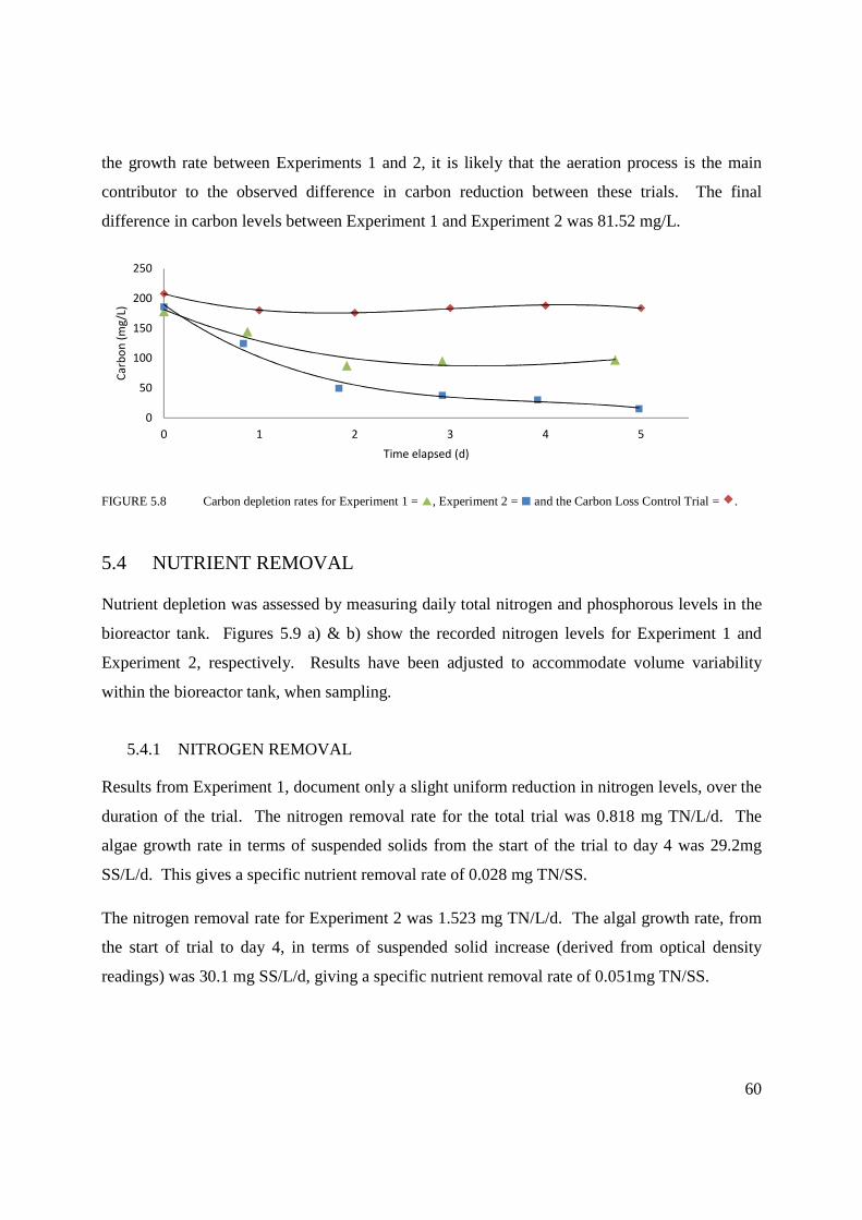
60

the growth rate between Experiments 1 and 2, it is likely that the aeration process is the main

contributor to the observed difference in carbon reduction between these trials. The final

difference in carbon levels between Experiment 1 and Experiment 2 was 81.52 mg/L.

FIGURE 5.8 Carbon depletion rates for Experiment 1 = �, Experiment 2 = � and the Carbon Loss Control Trial = �.


Nutrient depletion was assessed by measuring daily total nitrogen and phosphorous levels in the

bioreactor tank. Figures 5.9 a) & b) show the recorded nitrogen levels for Experiment 1 and

Experiment 2, respectively. Results have been adjusted to accommodate volume variability

within the bioreactor tank, when sampling.

5.4.1 NITROGEN REMOVAL

Results from Experiment 1, document only a slight uniform reduction in nitrogen levels, over the

duration of the trial. The nitrogen removal rate for the total trial was 0.818 mg TN/L/d. The

algae growth rate in terms of suspended solids from the start of the trial to day 4 was 29.2mg

SS/L/d. This gives a specific nutrient removal rate of 0.028 mg TN/SS.

The nitrogen removal rate for Experiment 2 was 1.523 mg TN/L/d. The algal growth rate, from

the start of trial to day 4, in terms of suspended solid increase (derived from optical density

readings) was 30.1 mg SS/L/d, giving a specific nutrient removal rate of 0.051mg TN/SS.

0

50

100

150

200

250

0 1 2 3 4 5

Ca

rbo

n (

mg

/L)

Time elapsed (d)

61

a) b)

FIGURE 5.9 a) & b) Nitrogen readings for (a) Experiment 1 (�) and (b) Experiment 2 (�)

5.4.2 PHOSPHOROUS REMOVAL

Figures 5.10 a) & b) show the recorded phosphorous levels for Experiment 1 and Experiment 2,

respectively. The phosphorous depletion rate for Experiment 1 was 0.362 mg/L/d giving a

specific growth rate of 0.012 P/SS. The ratio of phosphorous to nitrogen depletion was 362:818.

The phosphorous depletion rate of Experiment 2 was 0.381mg/L/d, with a specific growth rate of

0.013 P/SS, giving a P:N depletion rate of 381:1523.

The theoretical depletion rate of P:N is between 1:8 and 1:16 (Grobbellar 2004). Current results

range from 1:2 to 1:4, this is possibly due to poor correlation coefficient (r2) in fitting the graphs,

indicating that the consumption of N and P did not occur linearly throughout the experiment.

a) b)

FIGURE 5.10 a) & b) Phosphate readings for (a) Experiment 1 (�) and (b) Experiment 2 (�)

Slope = 0.8181 mg TN/L/d

R² = 0.0614

0

20

40

60

80

100

0 1 2 3 4 5

Nit

ron

ge

n (

mg

/L)

Time elapsed (d)

Slope =1.5227 mg TN/L/d

R² = 0.4296

0

20

40

60

80

100

0 1 2 3 4 5

Nit

rog

en

(m

g/L

)

Time elapsed (d)

Slope = 0.3617 mg P/L/d

R² = 0.4818

0

1

2

3

4

5

6

0 1 2 3 4 5

Ph

osp

ho

rou

s (m

g/L

)

Time elapsed (d)


R² = 0.792

0

1

2

3

4

5

6

7

0 1 2 3 4 5

Ph

osp

ho

rou

se (

mg

/L)

Time elapsed (d)

62

5.5 pH VARIATION

No CO2 addition was provided in either of the experiments. Therefore pH variability within the

bio-reactor, resulting from algal behaviour, was influenced predominantly by light source

availability. The light source was set on a 12hr on/off cycle. The controlled pH range was set at

7.7, with a tolerance of ±0.6, allowing a maximum pH value of 8.3. Fabergas et al. (1993)

suggests that algal strands can sequestrate bicarbonate (HCO3-) from a media up to a maximum

pH of 8.3, with optimal sequestration at 7.5.


The pH fluctuations for Experiment 1 are shown in Figure 5.11. pH levels rose steadily at all

identified growth phases. Dark (troughs) and light (peaks) periods are shown by the added red

line. Levels increased in dark and light phases, with predictably sharper rates of increase

observed during light periods. Within the lab setting, limited light source availability still existed

during the dark periods. The obtained results suggest that the algae Dunaliella tertiolecta still

had photosynthesis capacity under these limited light source conditions.

Figure 5.9 also suggest, a gradual reduction in the pH buffering capacity of the media.

Observable sudden drops in pH, resulted from the bioreactors automated system adding acid

when pH levels exceeded 8.3. As the trial progressed, the regulated acid input (10mL) generally

caused larger reductions in pH levels. Bicarbonate acts as a pH buffer, the higher the

bicarbonate concentration the higher the pH buffering capacity of a solution (Reference).

Therefore the observable loss of pH buffering capacity with time, suggests a reduction of the

media’s bicarbonate concentration.

63


Figure 5.12 shows the pH readings for days 1, 2, 3 & 4 of Experiment 1, over a 24 hour period.


respectively with the identified lag/exponential, linear, stationary and stationary/death growth

phases. All 24 hour readings start at midnight, splitting the dark period into two 6 hour sections.

The pattern of pH variability was characteristically similar for all growth phases of the

experiment, with steady rises in pH levels in the dark and light periods. For all readings, a slight

reduction in the pH gradient was generally observed when pH levels approached 8.3.

In the light periods, the sharpest increase in pH levels was observed on day 2 (linear),

approximately 0.073 pH unit/h. The shallowest light period gradient occurred on day 4

(stationary/death), approximately 0.036 pH unit/h. In the dark period, the steepest pH gradient

occurred at the end of day 2 (linear), approximately 0.047 pH unit/h, and the slowest pH increase

occurred at the end of day 4 (stationary/death), approximately 0.021 pH unit/h.

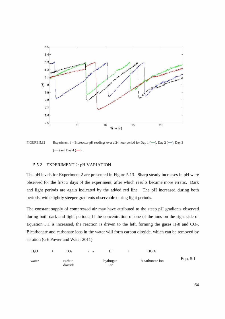
64

FIGURE 5.12 Experiment 1 – Bioreactor pH readings over a 24 hour period for Day 1 (―), Day 2 (―), Day 3

(―) and Day 4 (―).


The pH levels for Experiment 2 are presented in Figure 5.13. Sharp steady increases in pH were

observed for the first 3 days of the experiment, after which results became more erratic. Dark

and light periods are again indicated by the added red line. The pH increased during both

periods, with slightly steeper gradients observable during light periods.

The constant supply of compressed air may have attributed to the steep pH gradients observed

during both dark and light periods. If the concentration of one of the ions on the right side of

Equation 5.1 is increased, the reaction is driven to the left, forming the gases H20 and CO2.

Bicarbonate and carbonate ions in the water will form carbon dioxide, which can be removed by

aeration (GE Power and Water 2011).

H2O + CO2 « » H+ + HCO3-

water carbon dioxide

hydrogen ion

bicarbonate ion Eqn. 5.1

65

In this process, H+ will be removed (with HCO3-), and the removal of H+ will increase the pH of

the solution. This reduction in HCO3- is also supported by the TC measurements for Experiments

1 and 2. The timing within the trial of the sharper rates of loss of carbon from the media (Section

5.3.1) generally coincides with observed steeper pH gradients.

Assessing figure 5.13, the first 3 days coincide with the lag, exponential and linear growth

periods, as identified in Figure 5.3. Results for this period clearly demonstrated a steady

reduction in the buffering capacity as the trial progresses, suggesting a constant decline in the

bicarbonate concentration of the media. By day 4, the buffer capacity of the solution had

reduced to a level such that, the 10ml acid addition caused the pH to drop below the lower range

limit of 7.1, which led to the automated base addition. The acid/base input quantity was

subsequently adjusted to 6ml, steady results were achieved for the remainder of day 4. Minimal

pH variability was observed on day 5 (death phase).


Figure 5.14 shows the pH results over a 24 hour period for days 1, 2, 3 and 4, corresponding with

the identified lag/exponential, linear, stationary and stationary/death phases respectively. All 24

hour readings start at midnight, splitting the dark period into two 6 hour sections. Results show

relatively consistent pH patterns for all days, with the exception of day 4. A distinct change

66

(reduction) in the gradient, above a pH reading of 8 was frequently observable on the first 3 days

of the trial.

Significant increases in pH were observed in both dark and light periods. In the light periods the

steepest average pH gradients were observed on Day 1 (lag/exponential), approximately 0.331

pH unit/h. The shallowest average gradients occurred on Day 4 (stationary/death),

approximately 0.195 pH unit/h. In the dark period the steepest average pH gradient was

recorded at the start of day 1 (lag/exponential), approximately 0.109 pH unit/h. A negative pH

gradient was observed at the end of day 4 (stationary/death), approximately -0.042 pH unit/h.

FIGURE 5.14 Experiment 1 – Bioreactor pH readings over 24 hour period for Day 1 (―), Day 2 (―), Day 3

(―) and Day 4 (―).

5.5.3 pH VARIATION SUMMARY

The pH results of the 2 trials show significantly sharper increases in pH levels in Experiment 2.

The cause of this steeper gradient is likely due to a combination of algal growth and the removal

of H+ from the solution through carbon stripping.

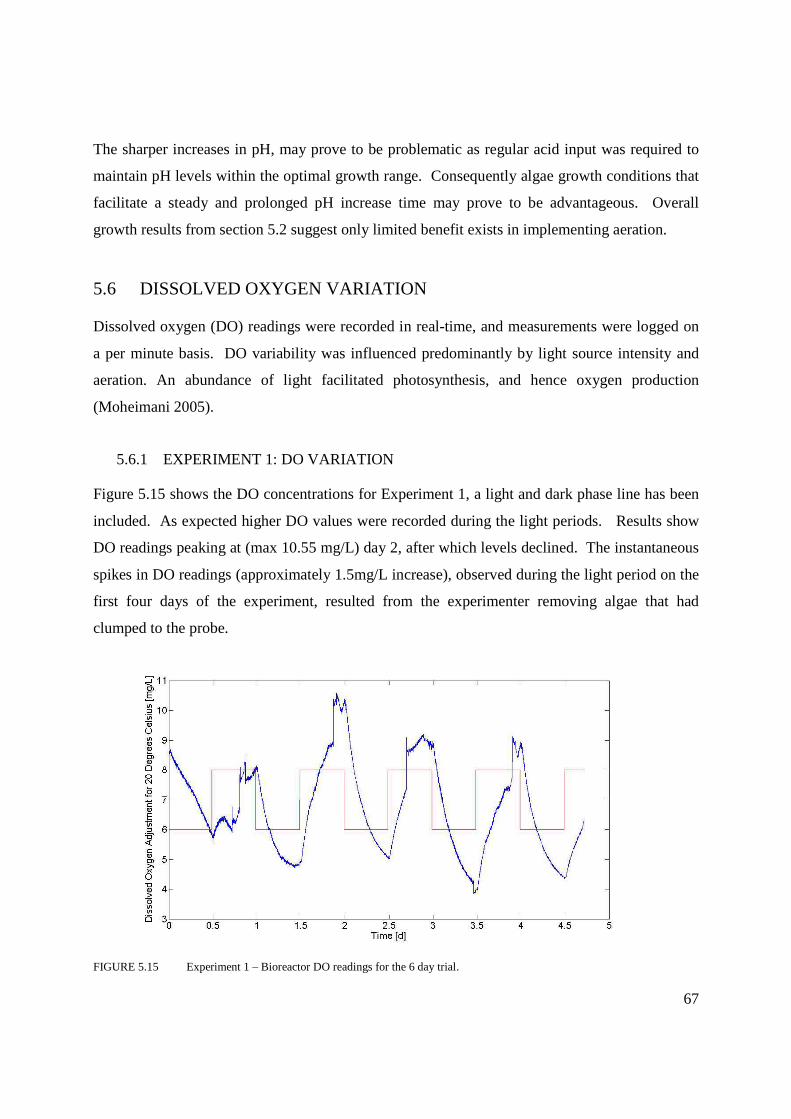
67

The sharper increases in pH, may prove to be problematic as regular acid input was required to

maintain pH levels within the optimal growth range. Consequently algae growth conditions that

facilitate a steady and prolonged pH increase time may prove to be advantageous. Overall

growth results from section 5.2 suggest only limited benefit exists in implementing aeration.


Dissolved oxygen (DO) readings were recorded in real-time, and measurements were logged on

a per minute basis. DO variability was influenced predominantly by light source intensity and

aeration. An abundance of light facilitated photosynthesis, and hence oxygen production

(Moheimani 2005).


Figure 5.15 shows the DO concentrations for Experiment 1, a light and dark phase line has been

included. As expected higher DO values were recorded during the light periods. Results show

DO readings peaking at (max 10.55 mg/L) day 2, after which levels declined. The instantaneous

spikes in DO readings (approximately 1.5mg/L increase), observed during the light period on the

first four days of the experiment, resulted from the experimenter removing algae that had

clumped to the probe.


68

Figure 5.16 compares average maximum DO readings during the light period with average

maximum DO readings in the dark period, for Experiment 1. The relative difference between

these two sets of values provides an estimate of the net oxygen produced during each of the light

periods. The saturation value of DO at 20°C is 9.17 mg/L, this is also indicated on the graph, as

is the measured optical density readings for this trial.


production levels increased until the end of day 2 (linear), before declining. This increase in DO

production is likely the result of a growing volume of active biomass during the lag, exponential

and linear phases.

FIGURE 5.16 Experiment 1 –Average maximum DO readings during light period (�), average minimum DO

readings during dark period (�), Net oxygen produced during the day time (Χ) and Optical

Density results (―).




0

0.02

0.04

0.06

0.08

0.1

0.12

0.14

0.16

0.18

0

2

4

6

8

10

12

14

0 1 2 3 4 5

Op

tica

l De

nsi

ty

Dis

solv

ed

Oxy

ge

n A

dju

ste

d f

or

20

De

gre

es

Ce

lsiu

s [m

g/L

]

Time Elaspe [d]

9.17mg DO/L

69




has been included. The results show an increase in DO readings until day 3 (max 8.35 mg/L),

followed by a rapid decline in DO variability as the trial reaches the death phase. The

instantaneous spikes in DO readings (approximately 1 to 1.5mg/L), observed during the first five

days of the experiment, resulted from the removal of algae that had clumped to the DO probe.


0.00

0.50

1.00

1.50

2.00

Pro

du

ced

Oxy

ge

n (

mg

)

Start Day 1 Day 2 Day 3 Day 4

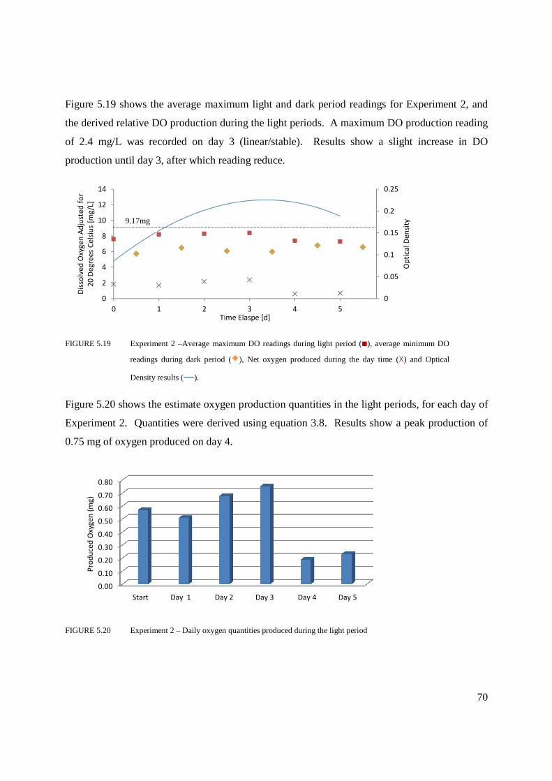
70

Figure 5.19 shows the average maximum light and dark period readings for Experiment 2, and

the derived relative DO production during the light periods. A maximum DO production reading

of 2.4 mg/L was recorded on day 3 (linear/stable). Results show a slight increase in DO

production until day 3, after which reading reduce.





Experiment 2. Quantities were derived using equation 3.8. Results show a peak production of

0.75 mg of oxygen produced on day 4.


0

0.05

0.1

0.15

0.2

0.25

0

2

4

6

8

10

12

14

0 1 2 3 4 5

Op

tica

l De

nsi

ty

Dis

solv

ed

Oxy

ge

n A

dju

ste

d f

or

20

De

gre

es

Ce

lsiu

s [m

g/L

]

Time Elaspe [d]

0.00

0.10

0.20

0.30

0.40

0.50

0.60

0.70

0.80

Pro

du

ced

Oxy

ge

n (

mg

)

Start Day 1 Day 2 Day 3 Day 4 Day 5

9.17mg

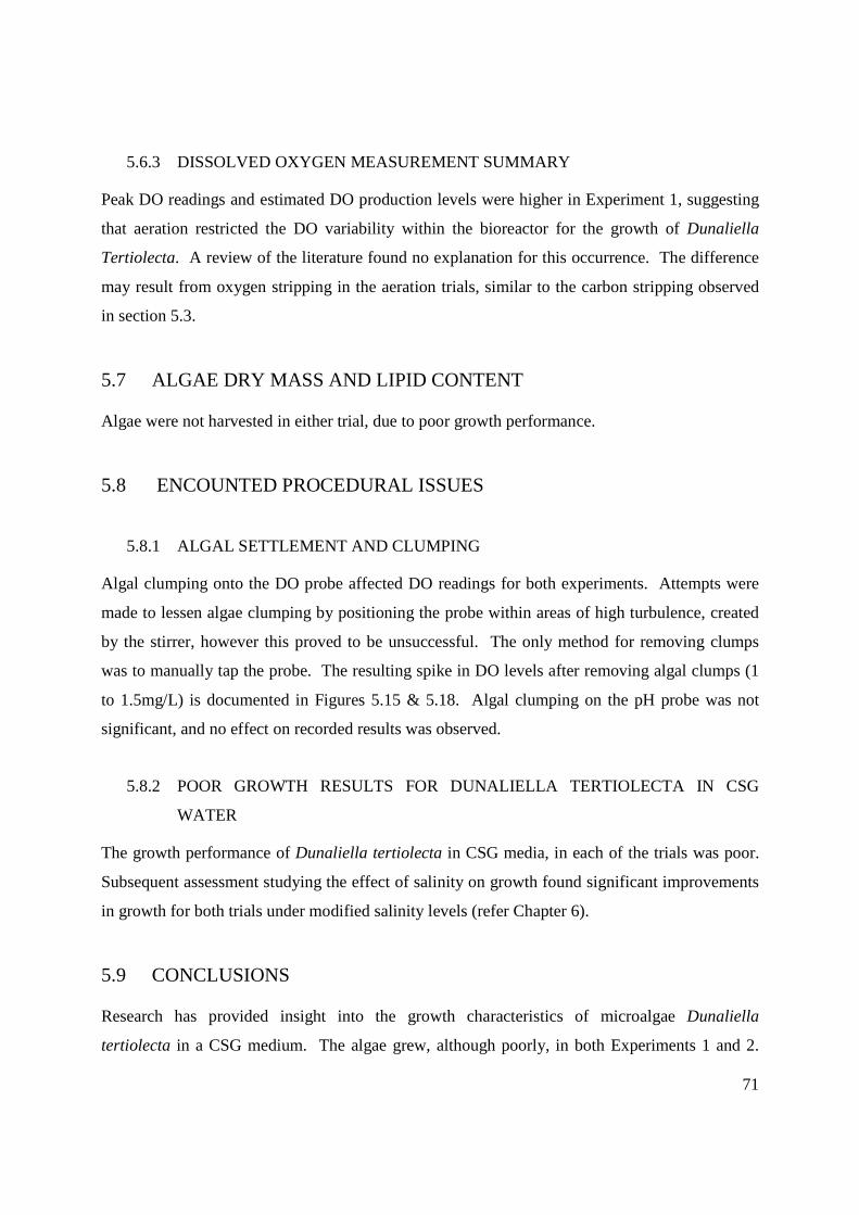
71

5.6.3 DISSOLVED OXYGEN MEASUREMENT SUMMARY

Peak DO readings and estimated DO production levels were higher in Experiment 1, suggesting

that aeration restricted the DO variability within the bioreactor for the growth of Dunaliella

Tertiolecta. A review of the literature found no explanation for this occurrence. The difference

may result from oxygen stripping in the aeration trials, similar to the carbon stripping observed

in section 5.3.


Algae were not harvested in either trial, due to poor growth performance.



Algal clumping onto the DO probe affected DO readings for both experiments. Attempts were

made to lessen algae clumping by positioning the probe within areas of high turbulence, created

by the stirrer, however this proved to be unsuccessful. The only method for removing clumps

was to manually tap the probe. The resulting spike in DO levels after removing algal clumps (1

to 1.5mg/L) is documented in Figures 5.15 & 5.18. Algal clumping on the pH probe was not

significant, and no effect on recorded results was observed.

5.8.2 POOR GROWTH RESULTS FOR DUNALIELLA TERTIOLECTA IN CSG

WATER

The growth performance of Dunaliella tertiolecta in CSG media, in each of the trials was poor.

Subsequent assessment studying the effect of salinity on growth found significant improvements

in growth for both trials under modified salinity levels (refer Chapter 6).

5.9 CONCLUSIONS

Research has provided insight into the growth characteristics of microalgae Dunaliella

tertiolecta in a CSG medium. The algae grew, although poorly, in both Experiments 1 and 2.

72

Optical density results suggest a slight overall benefit in aeration to facilitate the growth. The

assessment of pH variability found that aeration significantly increased the pH gradient, and this

was likely a result of the combination of algal growth and the removal of H+ through carbon

stripping. The subsequent steep rises in pH resulted in significant acid addition to moderate pH

levels. Furthermore, aeration was found to cause losses of carbon from the media through

stripping. Results suggest a potential for algal farming in CSG water without aeration.

73

CHAPTER 6 GROWTH CHARICTERISTICS AND LIPID

PRODUCTION OF MICROALGAE

DUNALLIELLA TERTIOLECTA GROWN IN

SALINITY MODIFIED CSG WATER MEDIA

AND THE EFFECTS OF AERATION.

This chapter presents the results and discussions on the optimal salinity, growth behaviour,

carbon sequestration and nutrient removal of Dunaliella Tertiolecta in CSG water, using batch

experiments. The discussions further extend to interpret the observations on real-time

monitoring using the dissolved oxygen and pH probes during the growth period. This chapter

ends with the assessment of lipid production from the harvested trials.

6.1 OPTIMAL SALINITY IDENTIFICATION

Initial assessment was made to identify the approximate optimal salinity level to facilitate growth

of Dunaliella tertiolecta in a CSG medium. Four batch trials were conducted with salinity levels

(NaCl) of 3.5g/L (CSG water), 10 g/L, 20 g/L and 35 g/L (seawater equivalent). At the

commencement of the trials 250 ml of CSG water with modified salinity levels, were inoculated

with 10 ml of Dunaleilla tertiolecta culture (0.28 mg of biomass), 5 ml/L of F2 concentrate and

1344mg/L of Sodium Bicarbonate (NaHCO3).

Trials were carried out simultaneously in 250ml flasks, over a 7 day period. Photo-energy was

provided by means of a light source, implemented on a 12 hour on (6am to 6pm) /off cycle.

Optical density reading results (Figure 6.1) show optimal growth was achieved in the 10g

NaCl/L trial. The trial with unmodified salinity levels (3.5g Nacl/L) performed comparatively

poorly. Therefore it was concluded from these preliminary investigations that Dunaliella

Tertiolecta would optimally grow in a salinity of 10 g/L, and subsequent trials were conducted

using the modified CSG water with 10 g NaCl/L.

74

FIGURE 6.1 Algal growth in CSG water media measured with Optical Density at 505 nm with salinity

levels of 3.5g NaCl/L (�), 10g NaCl/L (�), 20g NaCl/L (�) and 35g NaCl/L (�).


Batch experiments were repeated using microalgae Dunaliella Tertiolecta in a CSG water media,

with the modified salinity of 10g NaCl/L). Trials were differentiated by the inclusion of aeration

input in Experiment 4. The purpose of this distinction was twofold, to determine the effects of

aeration on algal growth, and to test for a carbon stripping effect through aeration.

6.2.1 EXPERIMENT 3 (SALINITY MODIFIED CSG WATER MEDIA – NON-

AERATION)

Experiment 3 was conducted to assess the growth capacity of microalgae Dunaliella Tertiolecta

in a salinity modified (10g NaCl/L) CSG water medium, without aeration input. The experiment

was intended as a lab scale assessment, to evaluate the algae’s capacity to be grown in an open

pond setting. Monitoring of growth and nutrient removal was conducted for the entirety of the

trial. Photo-energy required for the algal growth was provided by means of a light source,

implemented on a 12 hour on (6am to 6pm)/off cycle.

0

0.1

0.2

0.3

0.4

0.5

0.6

0 1 2 3 4 5 6 7

Op

tica

l De

nsi

ty

Time (d)

75


Dunaliella tertiolecta culture (0.193 g of biomass), 7.5 g/L of NaCl and 5 ml/L of F2

concentrate. Sodium Bicarbonate (NaHCO3) was added to the media (1344mg/L) to increase

carbon levels to average CSG water conditions. The resulting C:N:P ratio was 192:85:8.5. Refer

to Section 3.3 for further details.

6.2.2 EXPERIMENT 4 (SALINITY MODIFIED CSG WATER MEDIA – AERATION)

Experiments 4 replicated Experiment 3, except for the addition compressed air, which was fed

into the bioreactor at a constant rate of 250ml/min. It was predicted that growth, and subsequent

lipid production and nutrient removal would increase with a constant aeration feed.

Furthermore, it was hypothesised that aeration would significantly reduce bicarbonate levels

within the media through stripping. Refer to Section 1.7.4 for details of aeration properties.


Dunaliella tertiolecta culture (0.198 g of biomass), 7.5 g/L of NaCl and 5 ml/L of F2

concentrate. Sodium Bicarbonate (NaHCO3) was added to the media (1344mg/L) to increase

bicarbonate levels. The C:N:P ratio for the batch experiment was 192:85:8.5. Refer to Section

3.3 for further details.

6.3 ALGAL GROWTH

Algal growth was quantified using daily Spectrometer measurements. Photos were taken to

document the phase transition of algal growth.


Figure 6.2 shows the recorded growth trends of Dunaliella tertiolecta in Experiment 3,

represented through optical density measurements. The added trend line is based on a 3rd order

polynomial. Results suggest a lag phase occurring within the first day of the experiment. The

exponential growth period appears to take place between days 1 and 2, with a linear growth

phase from days 2 to 5. Results suggest a possible transition to the stationary phase at the end of

day 5. The trial was stopped for harvesting before the death phase was reached.

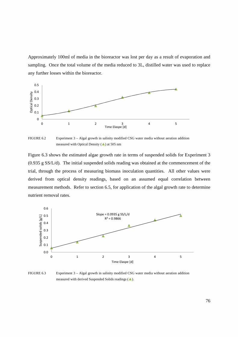
76

Approximately 100ml of media in the bioreactor was lost per day as a result of evaporation and

sampling. Once the total volume of the media reduced to 3L, distilled water was used to replace

any further losses within the bioreactor.

FIGURE 6.2 Experiment 3 – Algal growth in salinity modified CSG water media without aeration addition

measured with Optical Density (�) at 505 nm

Figure 6.3 shows the estimated algae growth rate in terms of suspended solids for Experiment 3

(0.935 g SS/L/d). The initial suspended solids reading was obtained at the commencement of the

trial, through the process of measuring biomass inoculation quantities. All other values were

derived from optical density readings, based on an assumed equal correlation between

measurement methods. Refer to section 6.5, for application of the algal growth rate to determine

nutrient removal rates.

FIGURE 6.3 Experiment 3 – Algal growth in salinity modified CSG water media without aeration addition

measured with derived Suspended Solids readings (�).

0

0.1

0.2

0.3

0.4

0.5

0 1 2 3 4 5

Op

tica

l De

nsi

ty

Time Elaspe [d]


R² = 0.9866

0.0

0.1

0.2

0.3

0.4

0.5

0.6

0 1 2 3 4 5

Susp

en

de

d s

olid

s [g

/L]

Time Elaspe [d]

77


Figure 6.4 shows the recorded growth characteristics of Dunaliella Tertiolecta with compressed

air input. The trend line was again derived using a 3rd order polynomial. The data suggests a

possible lag phase early on day 1, an exponential growth phase between days 1 to 3, and a linear

growth trend from day 3 to the end of the trial. The trial was stopped for harvesting before the

stationary and death phase were reached.

FIGURE 6.4 Experiment 4 - Algal growth in salinity modified CSG water media with aeration measured with

Optical Density (�) at 505 nm.

Figure 6.5 shows the estimated algae growth rate in terms of suspended solids for Experiment 4

(0.081 g SS/L/d). Refer to section 5.4, for application of the algal growth rate to determine

nutrient removal rates.

FIGURE 6.5 Experiment 4 – Algal growth in salinity modified CSG water media with aeration addition

measured with derived Suspended Solids readings (�)

0

0.1

0.2

0.3

0.4

0.5

0 1 2 3 4 5

Op

tica

l D

en

sity

Time Elaspe [d]


R² = 0.9876

0.0

0.1

0.2

0.3

0.4

0.5

0 1 2 3 4 5

Susp

en

de

d s

olid

s [g

/L]

Time Elaspe [d]

78

6.3.3 LOW BICARBONATE CONTROL TRIAL

A 5 day control trial with reduced bicarbonate levels was conducted to validate the benefit of

growing microalgae Dunaliella tertiolecta in a carbon rich solution. Refer to Section 6.3.4 for

growth results. The control trial replicated the parameters of Experiment 3, with the exception of

the reduced bicarbonate concentration of the media.

In preparation for the trial, 4 L of CSG media was aerated in the bioreactor tank for 3 days to

reduce the bicarbonate concentration of the solution. At the commencement of the trial the

carbon concentration was 33.6 mg C/L. No aeration was used during the trial period. Refer to

Section 6.4 for details of carbon variability during the trial.


Dunaliella Tertiolecta culture (0.245 g of biomass), 7.5 g/L of NaCl and 5 ml/L of F2

concentrate. The C:N:P ratio for the batch experiment was 33.6:85:8.5.


Comparison was made of the growth characteristics between Experiment 3, Experiment 4 and

the low bicarbonate control trial (Figure 6.6). Results show both Experiment 3 and 4 performing

significantly better than the control trial, indicating a distinct benefit in growing Dunaliella

tertiolecta in a carbon rich solution. Furthermore, growth measurements for Experiments 3 and

4 were comparatively similar, suggesting no identifiable benefit in implementing aeration.

FIGURE 6.6 Experiment 3, 4 & Low Bicarbonate Control Trial – Comparison of Dunaliellla tertiocleta growth in

a salinity modified CSG water media measured with Optical Density readings (Experiment 3 = �,

Experiment 4 = � and Low Bicarbonate Control Trial = � ) at 505 nm

0

0.1

0.2

0.3

0.4

0.5

0 1 2 3 4 5

Op

tica

l De

nsi

ty

Time Elaspe [d]

79

Figure 6.7 compares growth trends for Experiments 1, 2 in the salinity level 3.5g NaCl/L

(conducted in previous trials), with growth trends for Experiments 3 and 4, with salinity level 10

g NaCl/L. Results clearly demonstrate a benefit in increasing the salinity level to 10g NaCl/L.

The capacity for increasing the salinity levels in an outdoor pond setting could be achieved

through the implementation of reverse osmosis (RO) processes. Brine output from RO treatment

could be inputted into CSG water pond to increase salinity levels to optimise algal growth

conditions.

FIGURE 6.7 Experiment 1, 2, 3 and 4 – Comparison of Dunaliella tertiolecta growth in CSG water with salinity

levels 3.5g NaCl/L (Experiment 1 = � & Experiment 2 =�) and 10g NaCl/L (Experiment 3 = �

and Experiment 4 = �) measured with Optical Density readings at 505 nm

A comparison of the photographic documentation of Dunaliella Tertiolecta growth in the

bioreactor for Experiments 3, Experiment 4 and the low bicarbonate control trial is shown in

Figure 6.8. Photos illustrate high growth in both Experiments 3 & 4, and moderate growth in the

control trial (low bicarbonate).

0

0.1

0.2

0.3

0.4

0.5

0 1 2 3 4 5 6

Op

tica

l De

nsi

ty

Time Elaspe [d]

80

Experiment 3 (No Aeration)


Experiment 4 (Aeration)


Control Trial (Low Bicarbonate)


FIGURE 6.8 Photographic comparison of algae growth in the Bioreactor for Experiments 3, Experiment 4 and the

Low Carbon Control Trial over a 6 day trial period.

6.4 CARBON SEQUESTRATION

Carbon levels within the media were assessed through daily measurements of Total Carbon (TC),

using the Nitrogen Analyser (TOC-VCPH/CPN). Results for Experiments 3, 4 and the low

bicarbonate control trial are shown in Figures 6.9 a), b) and c) respectively. Readings have been

adjusted to accommodate tank volume variability, during sampling.

81

6.4.1 EXPERIMENTS 3, 4 AND CONTROL TRIAL: CARBON LEVELS

Recorded carbon levels in Experiment 3 were steady for the first day of the trail. After day 1

carbon levels decreased at a uniform rate for the remainder of the trial. The total carbon

reduction for this 4 day period was 120.9mg/L and the carbon removal rate was 29.29 mg C/L/d.

FIGURE 6.9 a) Total Carbon (TC) readings for Experiment 3

In Experiment 4, results show a steady decline in carbon levels over the first three days (148.3

mg/L reduction) coinciding with the identified lag, exponential and linear growth phases. The

carbon removal rate for this period was 49.4 mg C/L/d. Only a minimal carbon reduction was

recorded for the remainder of the trial (3.37 mg C/L) with a rate of reduction of 1.98 mg C/L/d.

FIGURE 6.9 b) Total Carbon (TC) readings for Experiment 4

In the control trial a steady decline in Carbon levels was observed over the first three days (29.1

mg/L reduction) coinciding with the identified lag, exponential and linear growth phases. The

carbon removal rate for this period was 9.1 mg C/L/d. No carbon reduction was recorded for the

remainder of the trial.

0

50

100

150

200

250

0 1 2 3 4 5

Ca

rbo

n (

mg

/L)

Time elapsed (d)

0

50

100

150

200

250

0 1 2 3 4 5

Ca

rbo

n (

mg

/L)

Time elapsed (d)

82

FIGURE 6.9 c) Total Carbon (TC) readings for the Low Bicarbonate Control Trial

6.4.2 CARBON SEQUESTION ASSESSMENT

Figure 6.10 shows the TC rates for Experiments 3, Experiment 4, the low bicarbonate control

trial and the carbon loss control trail (Section 5.3.2). Nutrient addition, algal inoculation and

salinity adjustment are the only differing factors between Experiment 3 and the carbon loss

control trial, therefore the resulting difference in carbon levels between the trials (82.2 mg/L) is

likely the result of carbon sequestration by the algae. Similarly, as there was no significant

difference in the growth rate between Experiments 3 and 4, it is likely that the aeration process is

the main contributor to the observed difference in carbon reduction between these trials. The

final difference in carbon levels between Experiment 3 and Experiment 4 was 72.40 mg/L.

FIGURE 6.10 Experiment 3, Experiment 4, Carbon Loss Control Trial and Low Bicarbonate Control Trial –

Carbon Depletion Rates (Experiment 3 =�, Experiment 4 = �, Carbon Loss Control Trial = � and

Low Bicarbonate Control Trial = �).

0

10

20

30

40

50

0 1 2 3 4 5

Ca

rbo

n (

mg

/L)

Time elapsed (d)

0

50

100

150

200

250

0 1 2 3 4 5 6

Ca

rob

on

(m

g/L

)

Time elapsed (d)

83


Nutrient depletion was assessed by measuring daily total nitrogen and phosphorous levels in the

bioreactor tank. Figures 6.11 a) & b) show the recorded nitrogen levels for Experiment 3 and

Experiment 4, respectively. Results have been adjusted to accommodate volume variability

within the bioreactor tank, when sampling.

6.5.1 NITROGEN REMOVAL

Results from Experiment 3, shows uniform reduction in nitrogen levels over the duration of the

trial period. The nitrogen removal rate for the total trial was 2.335 mg TN/L/d. The algae

growth rate in terms of suspended solids for Experiment 3 was 93.5 mg SS/L/d, giving a specific

nutrient removal rate of 0.025 mg TN/SS.

The nitrogen removal rate for Experiment 4 was 2.808 mg TN/L/d. The algal growth rate for

Experiment 4, in terms of suspended solid increase (derived from optical density readings) was

80.8 mg SS/L/d, giving a specific nutrient removal rate of 0.035mg TN/SS.

a) b)

FIGURE 6.11 a) & b) Nitrogen readings for (a) Experiment 3 (�) and (b) Experiment 4 (�)

6.5.2 PHOSPHOROUS REMOVAL

Figures 6.12 a) & b) show the recorded phosphorous levels for Experiment 3 and Experiment 4,

respectively. The phosphorous depletion rate for Experiment 3 was 1.156 mg/L/d giving a

specific growth rate of 0.012 P/SS. The ratio of phosphorous to nitrogen depletion was

Slope = 2.335

R² = 0.6592

0

10

20

30

40

50

60

70

0 1 2 3 4 5

Nit

rog

en

(m

g/L

)

Time elapsed (d)

Slope = 2.808

R² = 0.5831

0

10

20

30

40

50

60

0 1 2 3 4 5

Nit

rog

en

(m

g/L

)

Time elapsed (d)

84

1.156:2.335. The phosphorous depletion rate of Experiment 4 was 0.959mg/L/d, with a specific

growth rate of 0.012 P/SS, giving a P:N depletion rate of 0.959:2.808.

The theoretical depletion rate of P:N is between 1:8 and 1:16 (Grobbellar 2004). Current results

range from 1:2 to 1: 3, this is possibly due to poor correlation coefficient (r2) in fitting the graphs

especially for nitrogen depletion, indicating that the consumption of N and P did not occur

linearly throughout the experiments.

The observed low Phosphorous levels at the end of the trial period may have attributed to the

transition to a stationary phase, observed in experiment 3.

a) b)

FIGURE 6.12 a) & b) Phosphate readings for (a) Experiment 1 (�) and (b) Experiment 2 (�)

6.6 pH VARIATION

No CO2 addition was provided in Experiments 3 or 4. Therefore pH variability within the bio-

reactor, resulting from algal behaviour, was influenced predominantly by algal growth depending

on the light source availability. The light source was set on a 12hr on/off cycle. The controlled

pH range was set at 7.7, with a tolerance of ±0.6, allowing a maximum pH value of 8.3.


The pH fluctuations for Experiment 3 are shown in Figure 6.13. Dark (troughs) and light (peaks)

periods are shown by the added red line. In the light period, pH levels rose at an increasing rate

as the trial progressed. In the dark period a gradual increase in pH levels was observed on all

except the last day. The obtained dark period results, again suggested that the algae Dunaliella


R² = 0.9915

0

1

2

3

4

5

6

7

0 1 2 3 4 5

Ph

osp

ho

rou

s (m

g/L

)

Time elapsed (d)


R² = 0.9782

0

1

2

3

4

5

6

0 1 2 3 4 5

Nu

trie

nt

Am

ou

nt

(mg

/L)

Time elapsed (d)

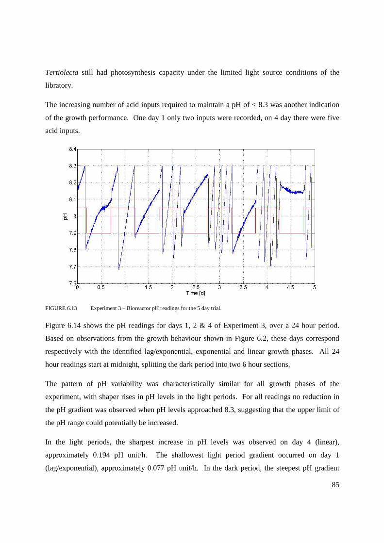
85

Tertiolecta still had photosynthesis capacity under the limited light source conditions of the

libratory.

The increasing number of acid inputs required to maintain a pH of < 8.3 was another indication

of the growth performance. One day 1 only two inputs were recorded, on 4 day there were five

acid inputs.


Figure 6.14 shows the pH readings for days 1, 2 & 4 of Experiment 3, over a 24 hour period.


respectively with the identified lag/exponential, exponential and linear growth phases. All 24

hour readings start at midnight, splitting the dark period into two 6 hour sections.

The pattern of pH variability was characteristically similar for all growth phases of the

experiment, with shaper rises in pH levels in the light periods. For all readings no reduction in

the pH gradient was observed when pH levels approached 8.3, suggesting that the upper limit of

the pH range could potentially be increased.

In the light periods, the sharpest increase in pH levels was observed on day 4 (linear),

approximately 0.194 pH unit/h. The shallowest light period gradient occurred on day 1

(lag/exponential), approximately 0.077 pH unit/h. In the dark period, the steepest pH gradient

86

occurred at the start of day 4 (linear), approximately 0.023 pH unit/h, a negative pH gradient was

observed at the end of day 4, approximately -0.005 pH unit/h. The Experiment 3 growth pattern

(Figure 6.2) suggests the alga is making a transition into the steady growth phase at this time

period.

FIGURE 6.14 Experiment 3 – Bioreactor pH readings over a 24 hour period for Day 1 (―), Day 2 (―), and

Day 4 (―).


The pH levels for Experiment 4 are presented in Figure 6.15. Sharp steady increases in pH were

observed for the first 3 days of the experiment. Dark and light periods are indicated by the added

red line. The pH increased during both periods until the end of day 3, with slightly steeper

gradients observable during light periods.

Similar to Experiment 2, the steep pH gradients observed in both the day and night periods, may

be attributable to a combined effect of algal growth and a reduction in H+ within the solution

resulting from carbon stripping through aeration. Refer to section 5.5.2 for further details.

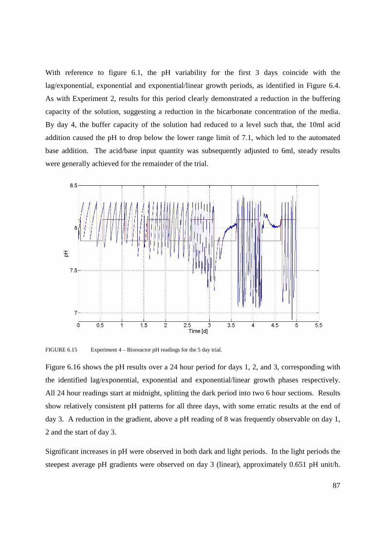
87

With reference to figure 6.1, the pH variability for the first 3 days coincide with the

lag/exponential, exponential and exponential/linear growth periods, as identified in Figure 6.4.

As with Experiment 2, results for this period clearly demonstrated a reduction in the buffering

capacity of the solution, suggesting a reduction in the bicarbonate concentration of the media.

By day 4, the buffer capacity of the solution had reduced to a level such that, the 10ml acid

addition caused the pH to drop below the lower range limit of 7.1, which led to the automated

base addition. The acid/base input quantity was subsequently adjusted to 6ml, steady results

were generally achieved for the remainder of the trial.


Figure 6.16 shows the pH results over a 24 hour period for days 1, 2, and 3, corresponding with

the identified lag/exponential, exponential and exponential/linear growth phases respectively.

All 24 hour readings start at midnight, splitting the dark period into two 6 hour sections. Results

show relatively consistent pH patterns for all three days, with some erratic results at the end of

day 3. A reduction in the gradient, above a pH reading of 8 was frequently observable on day 1,

2 and the start of day 3.

Significant increases in pH were observed in both dark and light periods. In the light periods the

steepest average pH gradients were observed on day 3 (linear), approximately 0.651 pH unit/h.

88

The shallowest average gradients occurred on day 1 (lag/exponential), approximately 0.099 pH

unit/h. In the dark period the steepest average pH gradient was recorded at the start of day 3

(linear), approximately 0.274 pH unit/h. The shallowest pH gradient was observed at the end of

day 3 (linear), approximately 0.194 pH unit/h.

FIGURE 6.16 Experiment 4 – Bioreactor pH readings over 24 hour period for Day 1 (―), Day 2 (―) and

Day 3 (―).

6.6.3 pH VARIATION SUMMARY

Similar to Section 5, the pH results of the 2 experiments show significantly sharper increases in

pH levels in aeration trial. The cause of this steeper gradient is likely due to a combination of

algal growth and the removal of H+ from the solution through carbon stripping.

The sharper increases in pH, may again prove to be problematic as significant acid input was

required to maintain pH levels within the optimal growth range. Consequently algae growth

conditions that facilitate a steady and prolonged pH increase time (Non-aeration trials) may

prove to be advantageous. Growth results from Section 6.3 suggest no overall benefit in

implementing aeration.

89


Dissolved oxygen (DO) readings were recorded in real-time, and measurements were logged on

a per minute basis. DO variability was influenced predominantly by light source intensity and

aeration. An abundance of light facilitated photosynthesis, and hence oxygen production

(Ferdnandes 2010).


Figure 6.17 shows the DO concentrations for Experiment 3, a light and dark phase line has been

included. As expected higher DO values were recorded during the light periods. Results show

DO readings peaking at 30.00 mg/L on days 3 and 4. Note that the upper limit reading capacity

of the dissolved oxygen meter (TPS 90-D) is 30.00 mg/L, suggesting that higher DO levels may

have occurred on these days due to extremely fast growing algae producing oxygen. Due to

these very high observed readings, a calibration check of the DO meter was conducted on day 3.

Calibration testing results suggested that the meter was functioning correctly.

The instantaneous spike in DO readings (approximately 2.5mg/L increase), observed during the

light period on the first day of the experiment, resulted from the experimenter removing algae

that had clumped to the probe.


90

Figure 6.18 compares average maximum DO readings during the light period with average

maximum DO readings in the dark period, for Experiment 3. The relative difference between

these two sets of values provides an estimate of the net oxygen produced during each of the light

periods. The saturation value of DO at 20°C is 9.17 mg/L, this is also indicated on the graph, as

is the measured optical density readings for this trial.


production levels increased until the end of day 3 (linear), before a suggested decline. This

increase in DO production is likely the result of a growing volume of active biomass during the

lag, exponential and linear phases.







0

0.05

0.1

0.15

0.2

0.25

0.3

0.35

0.4

0.45

0.5

0

5

10

15

20

25

30

35

0 1 2 3 4 5

Op

tica

l De

nsi

ty

Dis

solv

ed

Oxy

ge

n A

dju

ste

d f

or

20

De

gre

es

Ce

lsiu

s [m

g/L

]

Time Elaspe [d]

9.17mg

91

FIGURE 6.19 Experiment 3 – Daily oxygen quantities produced during the light periods



has been included. The results show an increase in DO readings until day 2 (max 10.5 mg/L),

followed by steady DO results for the remainder of the trial.


Figure 6.21 shows the average maximum light and dark period readings for Experiment 4, and

the derived relative DO production during the light periods. A maximum DO production reading

0.00

1.00

2.00

3.00

4.00

5.00

6.00

7.00

8.00

Pro

du

ced

Oxy

ge

n (

mg

)


92

of 3.7 mg/L was recorded on day 4(linear). Results show relatively stable DO production

throughout the trial period.





Experiment 4. Quantities were derived using equation 3.8. Results show a peak production of

1.04 mg of oxygen produced on day 4.

FIGURE 6.22 Experiment 4 – Daily oxygen quantities produced during the light periods

0

0.1

0.2

0.3

0.4

0.5

0

2

4

6

8

10

12

14

0 1 2 3 4 5

Op

tica

l De

nsi

ty

Dis

solv

ed

Oxy

ge

n A

dju

ste

d f

or

20

De

gre

es

Ce

lsiu

s [m

g/L

]

Time Elaspe [d]

0.00

0.20

0.40

0.60

0.80

1.00

1.20

Pro

du

ced

Oxy

ge

n (

mg

)


9.17mg

93

6.7.3 DISSOLVED OXYGEN MEASUREMENT SUMMARY

Peak DO readings and estimated DO production levels were significantly higher in Experiment

3, suggesting that aeration restricted the DO variability within the bioreactor for the growth of

Dunaliella tertiolecta. Results were similar to the findings in Section 5. The disparity of the DO

results could possibly be attributable to stripping of the oxygen through aeration, similar the

observed carbon stripping effect.


Algae were harvested after 5 days of growth. The algal dry mass and the total lipid content for

Experiment 3, Experiment 4 and the low carbon control trail are shown in Table 6.1. Results

indicate no definitive advantage between Experiment 3 and 4 processes. Furthermore results

further demonstrate the advantage of using a bicarbonate rich solution for oil production.

TABLE 6.1 Algal dry mass and lipid content

Trial Algal Dry Mass (g) Total Lipid Content (%)

Experiment 3 0.39 24

Experiment 4 0.41 20

Low Carbon Control Trial 0.28 25



Minimal algal clumping onto the DO probe, affecting DO readings was observed in the early

stages of Experiment 3. By positioning of the probe within the area of high turbulence created

by the stirrer, further clumping was avoided.

94

6.10 CONCLUSIONS

Research has provided insight into the growth characteristics of microalgae Dunaliella

tertiolecta in a salinity modified CSG medium. High growth rates were observed in both

Experiments 3 and 4, and moderate growth was observed in the low bicarbonate control trial.

Results suggest a clear benefit in adopting a bicarbonate rich solution for the growth of

Dunaliella tertiolecta. The assessment of pH variability found that aeration significantly

increased the pH gradient, and this was likely a result of the combination of algal growth and the

removal of H+ through carbon stripping. The subsequent steep rises in pH resulted in significant

acid addition to moderate pH levels. Furthermore, aeration was again found to cause large losses

of carbon from the media through stripping. Results suggest a potential for algal farming in CSG

water without aeration.

95

CHAPTER 7 CONCLUSIONS AND FUTURE WORK

7.1 CONCLUSIONS

The production of biofuel from microalgae can reduce greenhouse gas emissions, help address

future fuel shortages and create new industry in rural areas (CSIRO 2011). Over the next

decade, up to 300 GL of CSG water will be produced as a by-product of methane extraction

processes the in Surat and Bowen Basins. Typically this water is considered as a waste product

and is disposed of in large evaporation ponds. However, by utilizing a combination of high

carbon CSG water with nutrient rich agricultural waste to grow microalgae, there is the potential

to create significant quantities of biofuel (Pratt 2011).

In order to evaluate the capacity of utilising existing open pond infrastructure to grow algae in a

CSG water medium for the purpose of biofuel production, carbon sequestration and nutrient

extraction (nitrogen and phosphorous), lab scale batch experiments were conducted using

microalgae Dunaliella tertiolecta in this media, at the University of Southern Queensland. The

study has shown that Dunaliella tertiolecta can be grown in the CSG water, and there is a

capacity for lipid production, carbon sequestration and nutrient removal.

Initial trials using an unmodified CSG water sample with an F/2 nutrient supplement found poor

growth for non-aeration and aeration scenarios, with initial rates of 0.0292 g SS/L/d and 0.0303 g

SS/L/d, respectively. High growth was achieved once salinity levels were increased to 10 g

NaCl/L, with non-aeration growth rates of 0.0935 g SS/L/d and aeration growth rates of 0.0808 g

SS/L/d. Overall performance results indicated no clear benefit in adopting aeration for algal

growth facilitation. A control trial with a lowered bicarbonate concentration and salinity level of

10 g NaCl/L, found only moderate grow, suggesting a distinct benefit in utilizing a bicarbonate

rich solution for algal production.

Carbon sequestration levels were assessed for the non-aeration trials (Experiment 1 and

Experiment 3). Results indicated substantial carbon absorption by the alga in both trials, with

quantities of up to 90.9mg C/L for Experiment 1 and 82.2mg C/L for Experiment 3. Carbon

stripping quantities for the aeration trials were found to be as high as 81.52 mg/L and 72.4 mg/L,

96

for Experiment 2 and Experiment 4 respectively. Overall results indicated a clear benefit in

adopting a non-aeration setting for high levels of carbon sequestration and algal growth.

Nutrient removal rates were highest in the salinity modified trails, with nitrogen and

phosphorous removal rates of 2.335 mg N/L/d and 1.156 mg P/L/d for Experiment 3, and 2.808

mg N/L/d and 0.959 mg P/L/d for Experiment 4. Nutrient depletion P:N ratios of 1:2 to 1:3 were

observed.

The algal dry mass and lipid content for Experiment 3, Experiment 4 and the low carbon control

trial were 0.39 g at 24%, 0.41 g at 20% and 0.28 g at 25%, respectively.

Overall results indicate that high levels of algal growth, carbon sequestration and nutrient

removal are achievable in a salinity modified CSG water medium. Generally speaking this

research has proven to be very successful, warranting further study of algal growth, lipid

production, carbon sequestration and nutrient removal from a CSG water source.

7.2 SUGGESTIONS FOR FUTURE WORK

7.2.1 CLOSED LOOP AERATION SYSTEM

Building on from the assessment of the effect of aeration on carbon stripping, investigation could

be made of the potential advantage of adopting a closed loop aeration system to facilitate algal

growth. By creating a closed system, in which the air is recycled through the CSG water, it is

hypothesised that carbon concentrations within the air and water would soon equalise. Therefore

aeration could be used to stimulate growth without causing excessive carbon stripping.

Furthermore, if carbon levels in the air supply did increase, there is the additional possibility that

this air could aid to moderate pH levels within a solution.

A closed bio-reactor tank structure with a base inlet and top outlet, exists in the USQ (FoES)

Environmental Engineering laboratory. A vacuum pumping system with inlet and outlet tubes,

capable of running for extended period (> 1 week) would be required.

97

7.2.2 OPTIMAL BICARBONATE LEVEL IDENTIFICATION

It has been shown that algal growth is highly sensitive to the concentration level of CO2 input,

with poor growth in both low and high concentration settings (Tang el al. 2010). Developing on

from this finding, assessment could be made to identify the optimal bicarbonate concentration for

algal growth. This may not be practical for a batch experiment setup. Alternately bicarbonate

concentrations could be monitored and adjusted daily, for set period trials, with varying

bicarbonate levels tested.

7.2.3 ALTERNATE AGLAL STRAND ASSESSMENT

Due to budget and time constraints, only one algal strand was tested in the CSG water.

Furthermore, because the CSG water source was an untested media, the prominent reason for the

selection of microalgae Dunaliella tertiolecta was its hardy nature rather than its lipid production

capacity. As this research has shown healthy algal growth was achievable in the CSG media,

future studies may consider selecting an algal strand with great lipid production capacity.

7.2.4 IMPROVED pH CONTROL

The pH moderation system controlled by Labview, moderated pH levels by adding consecutive

acid/base inputs until the level of the media returned to within a specified range. The period

between consecutive inputs is equal to the time data logging period (1 minute for all trials).

This was an issue, as a lag period existed between acid/base addition and the resulting final pH

level of the media. This lag period could extend for up to 10 minutes. Consequently over-

adjustment of pH levels by the automated system was an ongoing issue.

A preferable system would be to have the set minimum time period between consecutive

acid/base inputs independent of the set time period between data logging. And to have the

capacity to manually change both settings, as required.

7.2.5 IMPROVED REACTOR DESIGN

Suggested modifications to the bio-reactor include, adopting a tank structure that allows for

better light penetration into the media. This would likely require a wide thin structure,

increasing the surface area to volume ratio. Secondly the existing small rotor used for mixing

98

could be replaced with a larger rotor system. This may alleviate problems with clumping to the

probes, and the rotation speed could be reduced, potentially improving algal survival rates.

7.2.6 FUTURE EXPERIEMENTS

Due to time constraints, and with the capacity to only run one batch experiment at a time, all

experiments were conducted only once. It was therefore difficult to draw definitive conclusions

from the obtained results. Future works that intend to build on from this research, should first

attempt to replicate the relevant trials.

7.3 SUMMARY

This chapter concluded the results of the dissertation and made suggestions for future research.

It was found that optimal growth of Dunalella tertiolecta in CSG water was achieved with a

modified salinity level of 10 mg NaCl/L. Furthermore results demonstrated a significantly

benefit in using a bicarbonate rich solution for algal growth. Aeration was shown to cause

carbon stripping and did not appear to increase the overall growth. High levels of carbon

sequestration and nutrient removal rates were documented. A number of future research

suggestions were made including creating a closed aeration loop system, identifying the optimal

bicarbonate level for algal growth, testing alternate algal strands, modifying the pH control

system and improving the bio-reactor design shape and stirring method to facilitate algal growth.

99

REFERENCES

Aguilera, J, Jimenez, C, Rodriguez-Maroto, JM, Niell, FX 1994, Influence of subsidiary energy

on growth of dunaliella viridis teodoresco: the role of extra energy in algal growth, Journal of

Applied Phycology, vol. 6, pp. 323-330.

Alanne, K, Saari, A 2005, Distributed energy generation and sustainable development,

Renewable and Sustainable Energy Review, vol. 10, pp. 539-558.

APHA 1995, Standard methods for the examination of water and wastewater, 19th Edition,

American Public Health Association, Washington, DC.

Australian Treasury 2011, Strong growth low pollution, modelling a carbon price, Australian

Government the Treasury, Retrieved August 5 2011, from

http://www.treasury.gov.au/carbonpricemodelling/content/report/09chapter5.asp

Barsanti, L, Gualtieri, P 2006, Algae: anatomy, biochemistry, and biotechnology, Taylor &

Francis Group, USA.

Boney, AD 1966, A biology of marine algae, Hutchinson Education LTD, London.

Brune, DE, Lundquist, TJ, Benemann, JR 2009, Microalgal biomass for greenhouse gas

reductions: potential for replacement of fossil fuels and animal feeds, Journal of Environmental

Engineering, pp. 1136-1144.

Camiro-Vargas, TK, Hernandez-Ayon, JM, Valenzuela-Espinoza E, Delgadillo-Hinojosa, F,

Cajal-Medrano, R 2005, Dissolved inorganic carbon uptake by rhodomonas sp. and isochrysis

aff. galbana determined by a potentiometric technique, Aquacultural Engineering, vol. 33, pp.

83-95.

Chen, M, Tang, H, Ma, H, Holland, TC, Simon, KY, Salley, SO 2011, Effect of nutrients on

growth and lipid accumulation in the green algae dunaliella tertiolecta, Bioresource Technology,

vol. 102, pp. 16549-1655.

100

Chi, Z, O’Fallon, JV, Chen, S 2011, Bicarbonate produced from carbon capture for algae culture,

Trends in Biotechnology, vol. 29, pp. 537-541.

Chisti, Y 2007, Bio-diesel from microalgae, Biotechnology Advances, vol. 25, no. 3, pp. 294-

306.

CSIRO 2011, Sustainable biomass production, CSIRO, Retrieved June 14 2011, from

http://www.csiro.au/science/Sustainable-Biomass-Production.html#1

Department of Environment and Resource Management 2010, Coal seam gas water management

policy, Queensland.

EOL 2011, Dunaliella tertiolecta bucher, Encyclopaedia of Life, Retrieved 5 October 2011,

from http://labs1.eol.org/pages/901806?text_id=6602203

Fabergas, J, Ferron, L, Gamallo, Y, Vecino, E, Otero, A, Herrero, C 1993, Improvement of

growth rate and cell productivity by aeration rate in cultures of the marine microalgae dunaliella

tertiolecta, Bioresource Technology, vol. 48, iss. 2, pp. 107-111.

Fazeli, MR, Tofighi, H, Samadi, N, Jamalifar, H 2006, Effects of salinity on β-carotene

production by Dunaliella tertiolecta DCCBC26 isolated from the urmia salt lake, north of iran,

Bioresource Technology, vol. 97, pp. 2453-2456

Fernandes, BD, Dragone, GM, Teixeira, JA, Vicente, AA 2010, Light regime characterization in

an airlift photobioreactor for production of microalgae with high starch content, Applied

Biochemical Technology, vol. 161, pp. 218-226.

Folch, J, Lees, M, Sloane Stanley, GH 1957, A simple method for the isolation and purification

of total lipids from animal tissues, Journal of Biology and Chemistry, vol. 226, pp. 497-509.

GE Power and Water 2011, Power and water: water processing technologies, chapter 4 –

aeration, Retrieved 26 October 2011,

http://www.gewater.com/handbook/ext_treatment/ch_4_aeration.jsp

101

Giordano, M, Beardall, J, Raven, JA 2005, CO2 concentrating mechanisms in algae:

mechanisms, environmental modulation, and evolution, Annual Review of Plant Biology, vol. 56,

pp. 99-131

Grobbelaar 2004, Algal nutrition, mineral nutrition, handbook of microalgal culture:

biotechnology and applied phycology, Carlton, Australia.

Groom, MJ, Elizabeth, MG, Townsend, PA 2008, Biofuel and biodiversity: principles for

creating better policies for biofuel production, Conservation Biology, vol. 22, no. 3, pp. 602-609.

Harrison, PJ & Berges JA 2005, ‘Marine culture media’, in R Andersen (eds), Algae culturing

techniques, Elsevier Inc, London

Harun, R, Davidson, M, Doyle, M, Gopiraj, R, Danquah, M, Forde, G 2011, Technoeconimic

analysis of an integrated microalgae photobioreactor, biodiesel and biogas production facility,

Biomass and Bioenergy, vol. 35, pp. 741-747.

Huerta, IE, Colman, B, Lubian, LM 2000, Active CO2 transport by three species of marine

microalgae, Journal of Phycology, vol. 36, pp. 314-320.

Janke, LS, White, AL 2003, Long-term hyposaline and hypersaline stresses produce distinct

antioxidant response in the marine algae dunaliella tertiolecta, Journal of Plant Physiology, vol.

160, pp. 1193-1202.

Kinnon, ECP, Golding, SD, Boreham, CJ, Baublys, KA, Esterle, JS 2010, Stable isotope and

water quality analysis of coal bed methane production waters and gases form the bowen basin,

australia, International Journal of Coal Geology, vol. 82, pp. 219-231.

Lundquist, TJ, 2006, Production of algae in conjunction with wastewater treatment, California

Polytechnic State University. Retrieved 15 May, 2011 from

http://www.docstoc.com/docs/2988054/Production-of-Algae-in-Conjunction-with-Waste-

Treatment-Tryg-J.

Masojidek, J, Koblizek, M, Torzillo, G 2004, ‘Photosynthesis in microalgae’, in A Richmond

(eds), Handbook of microalgal culture: biotechnology and applied phycology, Blackwell Science

Ltd, UK.

102

Mata, TM, Martins, AA, Caetano, NS 2010, Microalgae for biodiesel production and other

applications: A review, Renewable and Sustainable Energy Reviews, vol. 14, pp. 217-232.

Moheimani, NR 2005, The culture of coccolithophorid algae for carbon dioxide bioremediation.

Retrieved 10 January, 2011, from http://researchrepository.murdoch.edu.au/206/

Nichols, HW 1973, Handbookof Physological Methods, Ed. JR Stein, Cambridge University

Press, Cambridge.

Pratt, S, Keymer, P, Lant, P, Keller, J 2011 ‘The potential for generating algae derived biofuels

using coal seam gas water as the growth media’, Research Paper, University of Queensland.

Prescott, LM, Harley, JP, Klein, DA 1990, Microbiology, Brown Publishers, USA.

Pufelski, N 2010, 'How effective is microalgae treatment of different wastewaters for

simultaneous nutrient removal and lipid production for bio-fuel?', BEng thesis, University of

Southern Queensland, Toowoomba.

Rodriguez-Maroto, JM, Jimenez, C, Aguilera J, Niell, JA 2005, Air bubbling results in carbon

loss during microalgal cultivation in bicarbonate-enriched media: experimental data and process

modelling, Aquacultural Engineering, vol. 32, pp. 493-508.

Richmond, A 2004, Biological principals of mass cultivation, handbook of microalgal culture:

biotechnology and applied phycology, Blackwell Publishing, Carlton, Australia.

SARDI 2009, Algal production group, SARDI Aquatic Sciences, South Australian Research and

Development Institute. Retrieved July 15, 2011, from

http://www.sardi.sa.gov.au/aquaculture/aquaculture/algal_production_group

Singh, J, Gu, S 2010, Commercialization potential of microalgae for biofuels production,

Renewable and Sustainable Energy Reviews, vol. 14, pp. 2596-2610.

Stern N (2007) The Economics of Climate Change. HM Treasury, London.

Tang, H, Abunasser, N, Garcia, MED, Chen, M, Simon, KY, Salley, SO 2010, Potential of

microalgae oil from dunaliella tertiolecta as a feedstock for biodiesel, Applied Energy,

doi:10.1016/j.apenergy.2010.09.013

103

Tsukahara, K, Sawayama, S 2005, Liquid fuel production using microalgae, Journal of the Japan

Petroleum Institute, vol. 48, no. 5, pp. 251-259.

Watanabe, MM 2005, ‘Freshwater culture media’, in R Andersen (eds), Algae culturing

techniques, Elsevier Inc, London.

1

Appendix A


FACULTY OF ENGINEERING AND SURVEYING

ENG4111/4112 Research Project

PROJECT SPECIFICATION

FOR: DANIEL HARRINGTON

TOPIC: NUTRIENT REMOVAL FROM WASTEWATER BY MICROALGAE

FOR USE IN BIO-FUEL

SUPERVISOR: Vasantha Aravinthan

PROJECT AIM: The aim for this project is to determine the whether bio-diesel feedstock

Coal Seam Gas water could be use

Effect of varying salinity levels,

Programme: Issue A, 22nd March 2011

1. Research background information relating to: coal seam gas water, the process of

deriving bio-fuels from microalgae, and the properties of relevant microalgae strands.

2. Research and select a microalgae strand best suited to produce bio-fuel derived from a

CSG water medium.

3. Undertake laboratory analysis of

As time permits:

2

Appendix B

Manual Trail Logging Sample

Trial H - Dunaliella Teriolecta in CSG water con Sodium bicarbonate & Bubbles

time Day Date Tank

Volume (L) TOC/TN

Label Ion Spectrometer Comments

4:30 1 14/9/2011 3.35 H1,H2 H1,H2 0.058 Dillution x

4

5:30 2 15/9/11 3.45 H3,H4 H3,H4 0.131 Dillution x

4

3:00 3 16/9/2011 3.4 H5,H6 H5,H6 0.173 Dillution x

4

1:30 4 17/9/2011 3.48 H7,H8 H7,H8 0.263 Dillution x

4

12:00 5 18/9/2011 3.55 H9,H10 H9,H10 0.357 Dillution x

4

2:30 6 19/09/2011 3.6 H11,H12 H11,H12 0.444 Dillution x

4

Trial Stopped

Nutrient Adjustment Method - Sample

Nitrogen

Date Time Duration

Time

elaps.

(hrs, min)

Time

elaps. (d,

hrs)

Av.

Read.

(mg/L)

Reactor

Vol. (L)

Av.

Read.

(mg)

Unconsum.

(mg/L)

Consumed

(mg/L)

Nutrients

(mg/L)

8/30/2011 18:00 0 0:00 0:00:00 61 3.32 203.007 61.147 0.000 61.147

8/31/2011 15:00 21:00 21:00 0:21:00 50 3.30 163.536 61.517 11.961 49.186

9/1/2011 16:00 25:00 46:00 1:22:00 58 3.22 187.632 63.046 4.775 56.372

9/2/2011 16:00 24:00 70:00 2:22:00 49 3.15 155.245 64.447 15.163 45.984

9/4/2011 11:30 43:30 113:30 4:17:30 62 3 187.324 67.669 5.228 55.919

3

Appendix B

MATLAB SCRIPT SAMPLE

%Trial H - pH Comparison of stages over 24hr %lag %DO_lag = xlsread('Total_Trial_H.xlsx',1,'A3:A1555' ); %pH_lag = xlsread('Total_Trial_H.xlsx',1,'B498:B193 8'); time = xlsread( 'Total_Trial_H.xlsx' ,1, 'N2:N1466' ); %exponential %DO_expo = xlsread('Total_Trial_H.xlsx',1,'A1555:A2 980'); pH_expo = xlsread( 'Total_Trial_H.xlsx' ,1, 'B440:B1904' ); %linear %DO_linear = xlsread('Total_Trial_H.xlsx',1,'A2980: A13222'); pH_linear = xlsread( 'Total_Trial_H.xlsx' ,1, 'B1904:B3368' ); %stationary %DO_stationary = xlsread('Total_Trial_H.xlsx',1,'A1 3222:A33333'); pH_stationary = xlsread( 'Total_Trial_H.xlsx' ,1, 'B3368:B4832' ); %death %DO_death = xlsread('Total_Trial_H.xlsx',1,'A33333: A33406'); pH_death = xlsread( 'Total_Trial_H.xlsx' ,1, 'B4832:B6296' ); figure; plot(time,pH_expo, 'g' ) grid off hold on plot(time,pH_linear, 'b' ) plot(time,pH_stationary, 'k' ) %plot(time,pH_death,'r') set(gca, 'FontSize' ,16) xlabel( 'Time [hr]' , 'FontSize' ,16) ylabel( 'pH' , 'FontSize' ,16) axis([0 24 7 8.5])

csg water as a medium to grow marine …eprints.usq.edu.au/21946/1/harrington_2011.pdf · faculty...

Documents