csiro askap science data archive requirements and · pdf filecsiro askap science data archive...
TRANSCRIPT
`
CSIRO ASKAP Science Data ArchiveRequirements ASKAP-SW- Version 0.8 30 October 2013 Status: Draft document for distribution Authors: Jessica Chapman (CASS), Ben Humphreys (CASS), Matthew Whiting (CASS), Dan Miller (CSIRO IM&T), Ray Norris (CASS) Keywords: ASKAP, Data, Archives
ASKAP Science Data Archive: Requirements and Use Cases
-0017
30 October 2013
Status: Draft document for distribution
: Jessica Chapman (CASS), Ben Humphreys (CASS), Matthew Whiting (CASS), Dan Miller (CSIRO IM&T), Ray Norris (CASS)
Keywords: ASKAP, Data, Archives
: Jessica Chapman (CASS), Ben Humphreys (CASS), Matthew Whiting (CASS), Dan Miller (CSIRO IM&T), Ray Norris (CASS)

ASKAP-SW-0017 October 2013 Version 0.8
Enquiries should be addressed to: [email protected] Document history
REVISION DATE AUTHORS DESCRIPTION OF CHANGE 0.1 01 Jul 2008 Ray Norris Initial Version 0.2 19 Sep 2008 Ray Norris Updated draft version 0.3 18 Mar 2013 Jessica Chapman Document substantially rewritten and
updated. 0.4 18 March
2013 Jessica Chapman Ben Humphreys Matthew Whiting Ray Norris
Updated to include comments from B Humphreys, M Whiting and R Sault.
0.5 19 March 2013
Jessica Chapman Ben Humphreys Matthew Whiting Ray Norris
Limited distribution of this draft to participants of March 2013 data meeting.
0.8 October 2013 Jessica Chapman Limited distribution to CASDA team and CASS staff for comment. Updated the high-level requirements. Added use cases for the Survey Science Projects. Additional tables and information included.
0.8 Oct 2013 Jessica Chapman Updated following document review by James Dempsey, Phil Edwards, JC Guzman, Ian Heywood, Ben Humphreys, Arkadi Kosmynin, Dan Miller, Dave Morrison, Ray Norris, Angus Vickery
Copyright and Disclaimer
© 2013 CSIRO To the extent permitted by law, all rights are reserved and no part of this publication covered by copyright may be reproduced or copied in any form or by any means except with the written permission of CSIRO.
Important Disclaimer
CSIRO advises that the information contained in this publication comprises general statements based on scientific research. The reader is advised and needs to be aware that such information may be incomplete or unable to be used in any specific situation. No reliance or actions must therefore be made on that information without seeking prior expert professional, scientific and technical advice. To the extent permitted by law, CSIRO (including its employees and consultants) excludes all liability to any person for any consequences, including but not limited to all losses, damages, costs, expenses and any other compensation, arising directly or indirectly from using this publication (in part or in whole) and any information or material contained in it.

INTRODUCTION
3 ASKAP-SW-0017 October 2013
Contents
1. Introduction ...................................... .................................................................. 5
1.1 Summary ................................................................................................................... 5
1.2 Scope ........................................................................................................................ 5
1.3 Document versions .................................................................................................... 6
1.4 Glossary .................................................................................................................... 6
2. ASKAP Overview .................................... ........................................................... 9
2.1 ASKAP specification .................................................................................................. 9
2.2 Locations ................................................................................................................. 10
2.3 ASKAP timeline ....................................................................................................... 10
2.4 Telescope Operating System .................................................................................. 12
2.5 Central Processor .................................................................................................... 13
2.5.1 Data conditioning and calibration......................................................................... 13
2.5.2 Imaging pipelines................................................................................................. 14
2.5.3 Source detections ................................................................................................ 16
2.5.4 Data sizes and postage stamp image cubes ....................................................... 17
2.5.5 Simultaneous pipelines ........................................................................................ 19
2.6 Data levels ............................................................................................................... 19
2.6.1 Data Validation .................................................................................................... 20
3. ASKAP Operations and science ...................... ............................................... 21
3.1 ASKAP science observations .................................................................................. 21
3.2 Early Science .......................................................................................................... 22
3.3 Survey Science Projects ......................................................................................... 23
3.3.1 EMU .................................................................................................................... 23
3.3.2 POSSUM ............................................................................................................. 24
3.3.3 WALLABY ........................................................................................................... 24
3.3.4 DINGO ................................................................................................................. 25
3.3.5 FLASH ................................................................................................................. 26
3.3.6 GASKAP .............................................................................................................. 26
3.3.7 VAST ................................................................................................................... 27
3.3.8 COAST ................................................................................................................ 27
3.3.9 CRAFT ................................................................................................................ 29
3.3.10 VLBI ..................................................................................................................... 29
3.4 Guest Science Projects ........................................................................................... 30
3.5 Target of Opportunity observations ......................................................................... 30
4. The science archive ............................... .......................................................... 31
4.1 Overview .................................................................................................................. 31
4.2 Pawsey Centre Infrastructure .................................................................................. 32
4.3 Primary data products ............................................................................................. 34
4.4 Virtual Observatory protocols .................................................................................. 35
4.5 Data volumes .......................................................................................................... 35
5. Requirements and use cases ........................ .................................................. 38
5.1 Requirements .......................................................................................................... 38
5.2 Data access ............................................................................................................. 41
5.2.1 Low volume data access ..................................................................................... 41
5.2.2 High volume data access .................................................................................... 41
5.3 Survey Science Projects use cases ........................................................................ 41
5.4 Use cases for science users ................................................................................... 54
INTRODUCTION
4 ASKAP-SW-0017 October 2013
5.5 Use cases for Central Processor and archive administrators ................................. 56
Appendices ........................................ ....................................................................... 58
Appendix A: Data volumes ................................................................................................ 58
Appendix B: CASDA data products ................................................................................... 59
Appendix C: Survey parameters ........................................................................................ 61
References ........................................ ........................................................................ 71
INTRODUCTION
5 ASKAP-SW-0017 October 2013
1. INTRODUCTION
1.1 Summary
The CSIRO ASKAP Science Data Archive will provide the long term storage for ASKAP data products and the hardware and software facilities that enable astronomers to make use of these.
ASKAP is, in many ways, a data driven facility where the data rates are extremely high. The ASKAP data rates arriving at the Pawsey Centre are approximately 2.5 Gbytes per second, equivalent to 75 Petabytes (PB) per year. This is beyond the current ability to archive data and so raw visibility data and calibrated spectral line visibility data will not be archived. Such high data rates require instead that ASKAP data processing is carried out in quasi real time using automated pipelines to produce data products and associated metadata that are stored and made available through the science archive. The archive can be thought of as the end stage of the full system.
The CSIRO ASKAP Science Data Archive (hereafter CASDA) will include calibrated visibilities for continuum data, and image cubes for both spectral line and continuum data. Source detection algorithms will be used to search image cubes for radio sources and source-related information will be captured in catalogues. Calibration and scheduling information related to the observations will also be stored. The total volume of archive data is expected to reach 5 PB per year.
1.2 Scope
This document discusses the user requirements and use cases for CASDA as needed to support scientific observations with the ASKAP array located at the Murchison Radio Observatory (MRO). CASDA will provide the archive support from the start of Early Science onwards. Early Science will begin following the installation, commissioning and verification of the first 12 MkII phased array feeds (PAFs) on the antennas.
The document is written for a broad audience that includes ASKAP Survey Science Teams, the general astronomy community and groups from CASS, CSIRO IM&T, ICRAR and iVEC who are working on the radio astronomy archives at the Pawsey Centre. In particular, it is intended to provide the high level requirements and use cases to the CASDA development team as input for the more detailed design and architecture specifications, and is intended as a reference source for the Science Survey teams and general astronomy community to facilitate discussions towards verifying user requirements and use cases.
Some readers may not be familiar with ASKAP specifications, or with radio astronomy techniques. To help provide context, sections 2 and 3 provide an overview of the ASKAP system and operations. The science archive, requirements and use cases are discussed in sections 4 and 5.
In addition to CASDA, a separate commissioning archive will be used for the data collected from BETA – the initial array of six ASKAP antennas equipped with MkI PAFs. This archive

INTRODUCTION
6 ASKAP-SW-0017 October 2013
will also store and provide access to commissioning data as MkII PAFs are installed and tested on the antennas, and will include data from Early Science demonstrations. This archive is the responsibility of the CASS Science Data Processing group. The requirements of this commissioning archive are NOT discussed further in this document.
This document provides only minimal information on the User Support model for CASDA. This, together with performance measures for CASDA will be discussed in a separate document.
1.3 Document versions
This document draws strongly on previous ASKAP documents. In particular it builds on and replaces the earlier document ASKAP Science Data Archive: Draft Requirements Document (2009, Norris and Johnston [6]) and has made extensive use of ASKAP Science Processing (2011, Cornwell et al. [2]).
Version 0.5 of this document was released in March 2013 to facilitate discussions between CASS staff working on ASKAP and other technical groups.
This version (version 0.8) is released in October 2013, primarily for discussion with the science community. Following input from the community, Version 1.0 will be completed in late 2013.
1.4 Glossary
Acronym Definition
AAO Australian Astronomical Observatory
ADE ASKAP Design Enhancements
ANDS Australian National Data Service
ARCS Australian Research Collaboration Service
ARDC Australian Research Data Commons
ARRC Australian Resources Research Centre
ASKAP Australian SKA Pathfinder
ATOA Australia Telescope Online Archive
ATNF Australia Telescope National Facility
BETA Boolardy Engineering Test Array
CASA Common Astronomy Software Applications
CASS CSIRO Astronomy and Space Science
CASDA CSIRO ASKAP Science Data Archive
CPU Central Processing Unit
DAE Data Analysis Engine
DIRP Data Intensive Research Pathfinder
DMF Data Management Framework

INTRODUCTION
7 ASKAP-SW-0017 October 2013
DML Data Management Layer
DRAO Dominion Radio Astrophysical Observatory
EIF Education Investment Fund
FITS Flexible Image Transport System
FLOPS Floating Point Operations per Second
FWHM Full width at half maximum
GAMA Galaxy and Mass Assembly [survey]
Gb Gigabit (109 bits)
Gbps Gigabits per second
GB Gigabyte (109 bytes)
GBps Gigabytes per second
GPU Graphical Processing Unit
GSP Guest Science Project
HPC High Performance Computing
HSM Hierarchical Storage Management System
ICRAR International Centre for Radio Astronomy Research
IM&T Information Management and Technology
iVEC iVEC is an unincorporated joint venture between CSIRO, Curtin University, Edith Cowan University, Murdoch University and the University of Western Australia
IVOA International Virtual Observatory Alliance
LBA Long Baseline Array
MAID Massive Array of Idle Disks
MB Megabyte (106 bytes)
MRO Murchison Radio Observatory
MWA Murchison Widefield Array
NCI National Computing Infrastructure
NCMAS National Computational Merit Allocation Scheme
NCRIS
National Collaborative Research Infrastructure Strategy
NED NASA/IPAC Extragalactic Database
OPAL Online Proposal Applications and Links
PAF Phased Array Feed
PB Petabyte (1015 bytes)
PSF Point Spread Function
RDS Research Data Services
RDSI Research Data Storage Infrastructure
RFI Radio Frequency Interference
RTC Real Time Computer
INTRODUCTION
8 ASKAP-SW-0017 October 2013
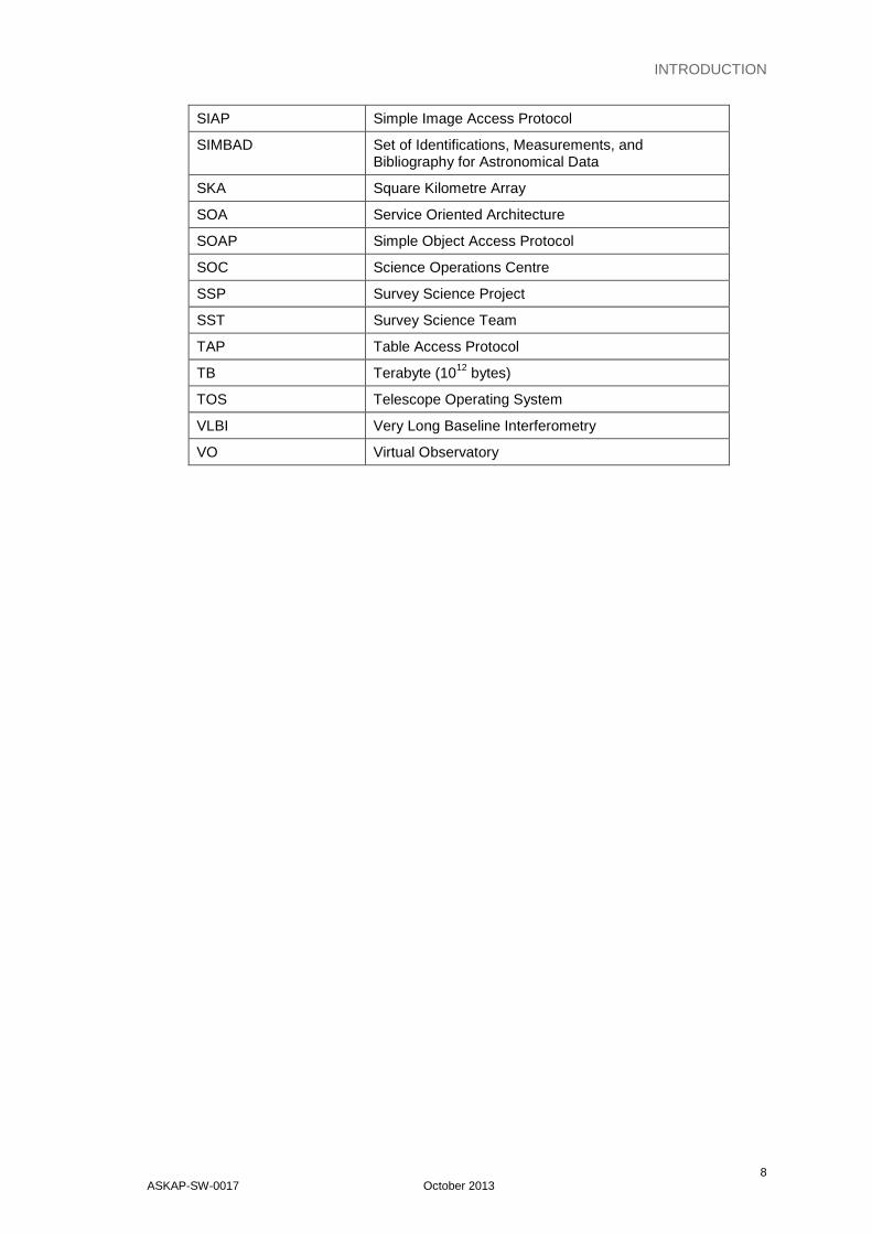
SIAP Simple Image Access Protocol
SIMBAD Set of Identifications, Measurements, and Bibliography for Astronomical Data
SKA Square Kilometre Array
SOA Service Oriented Architecture
SOAP Simple Object Access Protocol
SOC Science Operations Centre
SSP Survey Science Project
SST Survey Science Team
TAP Table Access Protocol
TB Terabyte (1012 bytes)
TOS Telescope Operating System
VLBI Very Long Baseline Interferometry
VO Virtual Observatory

ASKAP OVERVIEW
9 ASKAP-SW-0017 October 2013
2. ASKAP OVERVIEW
2.1 ASKAP specification
This section gives an overview of the ASKAP system. This is largely extracted from previous ASKAP documents [2, 4, 5].
ASKAP is an array of 36 12-m diameter prime-focus parabolic dish antennas located at the Murchison Radio Observatory in Western Australia. The array is designed to be a fast survey instrument for centimetre-wavelength observations with high dynamic range and a wide field-of-view.
The ASKAP system specification is given in Table 1.
Table 1: ASKAP specification
Number of antennas 36 Notes
Dish diameter 12 m Corresponds to a full-width half maximum primary beam of approximately one degree.
Maximum baseline 6 km 30 antennas are located within a region of 2 km in diameter. The remaining 6 extend the baselines to a maximum of 6 km.
Frequency range 700 – 1800 MHz Equivalent to approximately 42 cm (700 MHz) to 17 cm (1800 MHz)
Field-of-view (area) 30 square degrees
Processed bandwidth 300 MHz
Number of channels 16200 18.5 kHz per channel
Correlator integration time
5 s Minimum time per visibility sample
Number of Phased Array Feed elements
188 The number of elements for Mk II PAFs
Digitisation levels 14 bits
Dynamic range 50 dB
Sensitivity (Ae/Tsys) 65 m2 K-1
Survey speed 1.3 x 10⁵ m4 K-2 deg2

ASKAP OVERVIEW
10 ASKAP-SW-0017 October 2013
2.2 Locations
Physical locations for ASKAP sub-systems are:
• The antennas, beamformers and the correlator are located at the Murchison Radio Observatory (MRO).
• Operational engineering support is provided by CSIRO Astronomy and Space Science (CASS) staff located in Geraldton with some additional support provided from technical staff in Marsfield, Sydney.
• Data are transmitted over high-speed dedicated links to the Pawsey Centre in Perth.
• The Central Processor used for real-time data processing is located at the Pawsey Centre. The platform within the Pawsey Centre which hosts the Central Processor is known as the Real Time Computer.
• CASDA will be located at the Pawsey Centre.
• The CASDA development team includes CSIRO staff from CASS and IM&T located in Canberra and Sydney, with support from iVEC in Perth.
• In the future it is possible that one or more mirrors of the archive may be located at other locations although this is not yet established.
• ASKAP observations will normally be carried out and monitored by CASS Science Operations staff located at the CASS Science Operations Centre in Marsfield, Sydney.
• First-level user support for the archive will be provided by CASS Science Operations.
• ASKAP will also provide data used for education and outreach programmes. The coordination of these programmes will be from the CASS Headquarters, in Sydney.
2.3 ASKAP timeline
Figure 1 shows an overview and timeline for major ASKAP activities. As at mid-October 2013:
• The site infrastructure including roads, a RFI-shielded control building, waste, water, initial power and fibre links are complete.
• The installation of the 36 ASKAP antennas is complete.
• MkI Phased Array Feeds (PAFs) are installed on the BETA array. BETA is primarily be used for development and commissioning purposes.
• MkII PAFs are under development with the production of the first full MkII PAF in 2013.
• Installation, commissioning and science verification of the MkII PAFs will continue throughout 2014.
• Early Science with ASKAP will begin following the commissioning and science verification of the first 12 MkII PAFs.
• Further MkII PAFs will be added to the array during 2015.

ASKAP OVERVIEW
11 ASKAP-SW-0017 October 2013
• Fibre links to the Pawsey Centre will have data rates of 40 Gb/s in the near future.
• The Pawsey Centre building was completed in April 2013 and installation of a Cray supercomputer and storage facilities began soon after. Installation and acceptance tests are underway.
• Planning for the science archive has begun. It is intended that CASDA will be available from the start of Early Science around early 2015.
Figure 1: ASKAP timeline

ASKAP OVERVIEW
12 ASKAP-SW-0017 October 2013
2.4 Telescope Operating System
Figure 2 summarises the ASKAP data flow.
Figure 2: ASKAP data flow (adapted from [1])
The ASKAP computing architecture has three major components: the Telescope Operating System, the Central Processor and CASDA. The Telescope Operating System is responsible for the control and monitoring of the antennas. This includes the antennas, beamformers and correlator.
The ASKAP large field of view is achieved using phased array feeds with 188 detection elements at the focus of the antennas. For each antenna the voltages measured by these elements are amplified, digitised and filtered into 304 coarse channels of 1 MHz each.
The beamformer for an antenna constructs beams by summing and weighting the signals from the individual elements. ASKAP will be configured to give a total of 36 observing beams.
The samples for each beam are further filtered to high resolution. Each 1 MHz channel is split into 54 fine channels, giving 16,416 channels in total. Edge channels are later discarded and a total bandwidth of 300 MHz and 16,200 channels are used.
The signals from one antenna beam are correlated with the signals from the corresponding beams from the other antennas. In effect this allows ASKAP to operate in a way that is equivalent to a number of conventional radio arrays operating simultaneously. The correlator forms the cross-products between each pair of antennas. ASKAP antennas have two linear polarisation axes allowing four polarisation products (called XX, YY, XY and YX). For each integration period of 5 seconds, one cross-correlation (also called a ‘visibility’) is output from the correlator for each beam, baseline, channel and polarisation. The correlator also outputs one auto-correlation for each beam, antenna, channel and polarisation.
For 36 beams, 630 baselines, 36 autocorrelations, four polarisation products and 16,416 channels the correlator produces 1.6 billion distinct correlations and a total data volume, every

ASKAP OVERVIEW
13 ASKAP-SW-0017 October 2013
5 seconds, of 12.6 Gigabytes (GB). Thus the maximum data rate from the correlator, for a full array of 36 antennas is 2.5 Gigabytes per second (GBps). For a smaller number of antennas the data rate scales as the number of baselines. During the data processing stages the data volumes are reduced.
The correlation samples are then sent over high speed links to the Pawsey Centre at the maximum data rate of 2.5 GBps. Four 10 Gigabits per second (Gbps) links will be available for ASKAP.
2.5 Central Processor
The Central Processor is a hardware and software subsystem that is responsible for all of the stages of data processing from the correlator to the production of science data products such as image cubes and source catalogues. The processor as a system can be thought of as a sophisticated ‘backend’ to the array.
The processor includes a Cray supercomputer with 9,440 Central Processing Unit (CPU) cores, a total memory of 32 TB and a total compute power of 200 TFLOPS. This is supported by a 1.4 PB Lustre disk-based file system that is used to buffer the visibility data during data processing and to temporarily store the data products produced prior to sending these to the archive.
2.5.1 Data conditioning and calibration
Data processing is carried out using a set of pipelines. A schematic of the data conditioner pipeline (also known as the ingest pipeline) is shown in Figure 4.
Figure 3: Data Conditioner Pipeline
Data arriving from the correlator are acquired through a set of 16 ingest nodes and merged with telescope-related metadata provided by the Telescope Operating System. The data are then ‘conditioned’ prior to being forwarded to the science processing pipelines. Conditioning steps
Services
Ingest Pipeline
Merge Metadata & Visibilities
Correlator
Telescope Observation
ManagerTelescopemetadata
Visibilities
RFI Source Service
Calibration Data
Service
Apply Calibration
Flag(On the fly detection)
Flag(From RFI database)
Channel Averaging
(16200 to 300)
Channel Averaging
(300 to ~30)Access database ofknown RFI sources
Obtain latestcalibration solution
Downstream Pipelines
Downstream Pipelines
Downstream Pipelines
Calibrated visibilities
Calibrated visibilities
Calibrated visibilities
ASKAP OVERVIEW
14 ASKAP-SW-0017 October 2013
include flagging the data for known sources of radio frequency interference (RFI). This is done using a database of known interference sources as well as the dynamic detection of new interference sources. Other bad data are also flagged.
After conditioning, the visibilities are calibrated to correct for atmospheric and instrumental visibility variations and for the instrumental bandpasses. The calibration of ASKAP data with many beams requires a novel approach to data calibration. The full ASKAP array will use a self calibration technique where a pre-determined global model of the sky, based on information derived from known bright sources, is used to correct the observed visibilities. This model will be updated and improved as ASKAP observations progress [2]. During commissioning and Early Science where a smaller number of antennas are used, alternative calibration methods may be applied. After calibration the data are averaged as needed and the calibrated visibilities are sent to imaging pipelines.
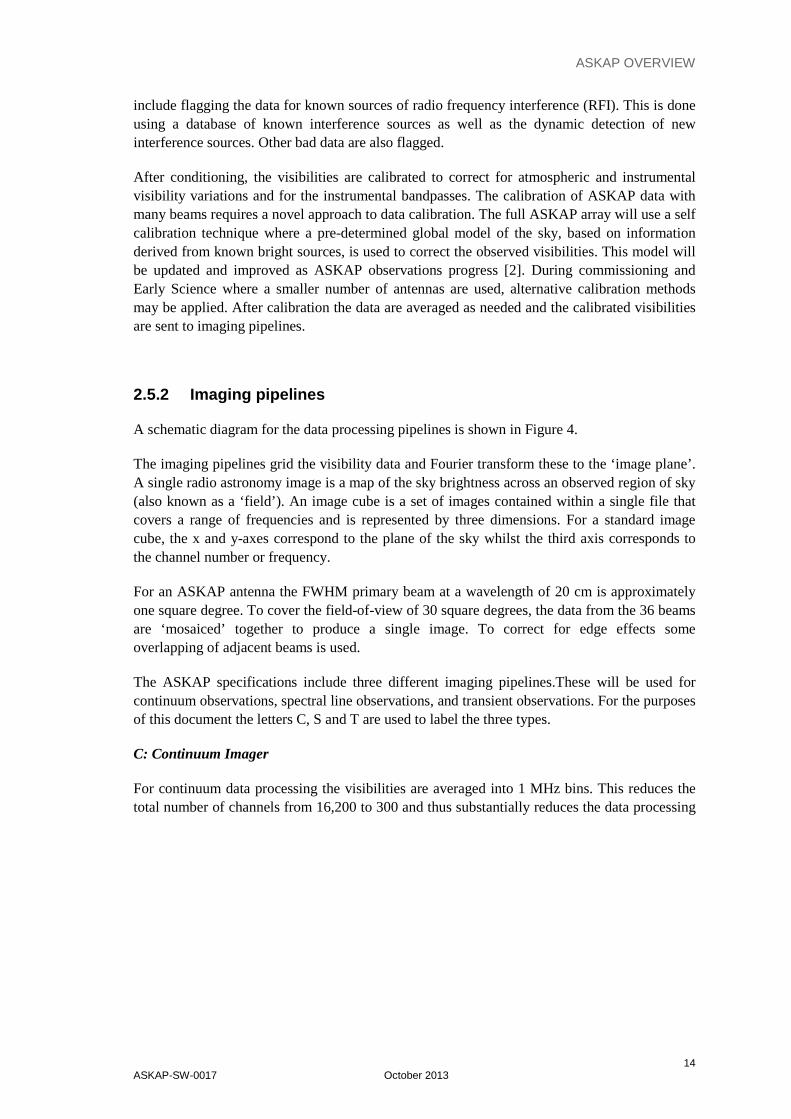
2.5.2 Imaging pipelines
A schematic diagram for the data processing pipelines is shown in Figure 4.
The imaging pipelines grid the visibility data and Fourier transform these to the ‘image plane’. A single radio astronomy image is a map of the sky brightness across an observed region of sky (also known as a ‘field’). An image cube is a set of images contained within a single file that covers a range of frequencies and is represented by three dimensions. For a standard image cube, the x and y-axes correspond to the plane of the sky whilst the third axis corresponds to the channel number or frequency.
For an ASKAP antenna the FWHM primary beam at a wavelength of 20 cm is approximately one square degree. To cover the field-of-view of 30 square degrees, the data from the 36 beams are ‘mosaiced’ together to produce a single image. To correct for edge effects some overlapping of adjacent beams is used.
The ASKAP specifications include three different imaging pipelines.These will be used for continuum observations, spectral line observations, and transient observations. For the purposes of this document the letters C, S and T are used to label the three types.
C: Continuum Imager
For continuum data processing the visibilities are averaged into 1 MHz bins. This reduces the total number of channels from 16,200 to 300 and thus substantially reduces the data processing
ASKAP OVERVIEW
15 ASKAP-SW-0017 October 2013
load. Further averaging may be applied. Continuum imaging will generally use one of two modes:
All 300 channels are retained and the data products formed are continuum image cubes. Image cubes may be retained for all four polarisation products known as Stokes I (total intensity), Q (linear polarisation), U (linear polarisation), and V (circular polarisation).
A ‘multi-frequency synthesis’ technique is used where the full set of frequency information is used to produce images for three ‘Taylor terms’. These correspond to the source flux density at a given frequency, the spectral index and the spectral curvature1.
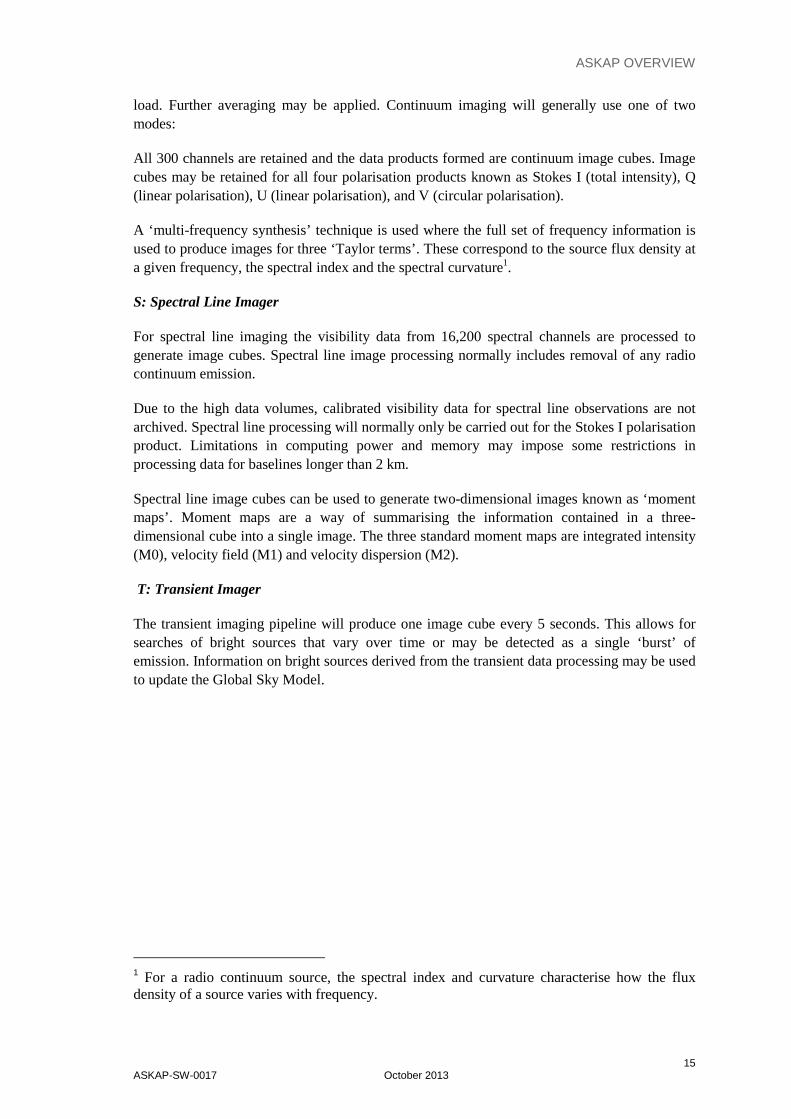
S: Spectral Line Imager
For spectral line imaging the visibility data from 16,200 spectral channels are processed to generate image cubes. Spectral line image processing normally includes removal of any radio continuum emission.
Due to the high data volumes, calibrated visibility data for spectral line observations are not archived. Spectral line processing will normally only be carried out for the Stokes I polarisation product. Limitations in computing power and memory may impose some restrictions in processing data for baselines longer than 2 km.
Spectral line image cubes can be used to generate two-dimensional images known as ‘moment maps’. Moment maps are a way of summarising the information contained in a three-dimensional cube into a single image. The three standard moment maps are integrated intensity (M0), velocity field (M1) and velocity dispersion (M2).
T: Transient Imager
The transient imaging pipeline will produce one image cube every 5 seconds. This allows for searches of bright sources that vary over time or may be detected as a single ‘burst’ of emission. Information on bright sources derived from the transient data processing may be used to update the Global Sky Model.
INTRODUCTION
INTRODUCTION
ERROR! NO TEXT OF SPECIFIED STYLE IN DOCUMENT.
ERROR! NO TEXT OF SPECIFIED STYLE IN DOCUMENT.
1 For a radio continuum source, the spectral index and curvature characterise how the flux density of a source varies with frequency.
ASKAP OVERVIEW
16 ASKAP-SW-0017 October 2013
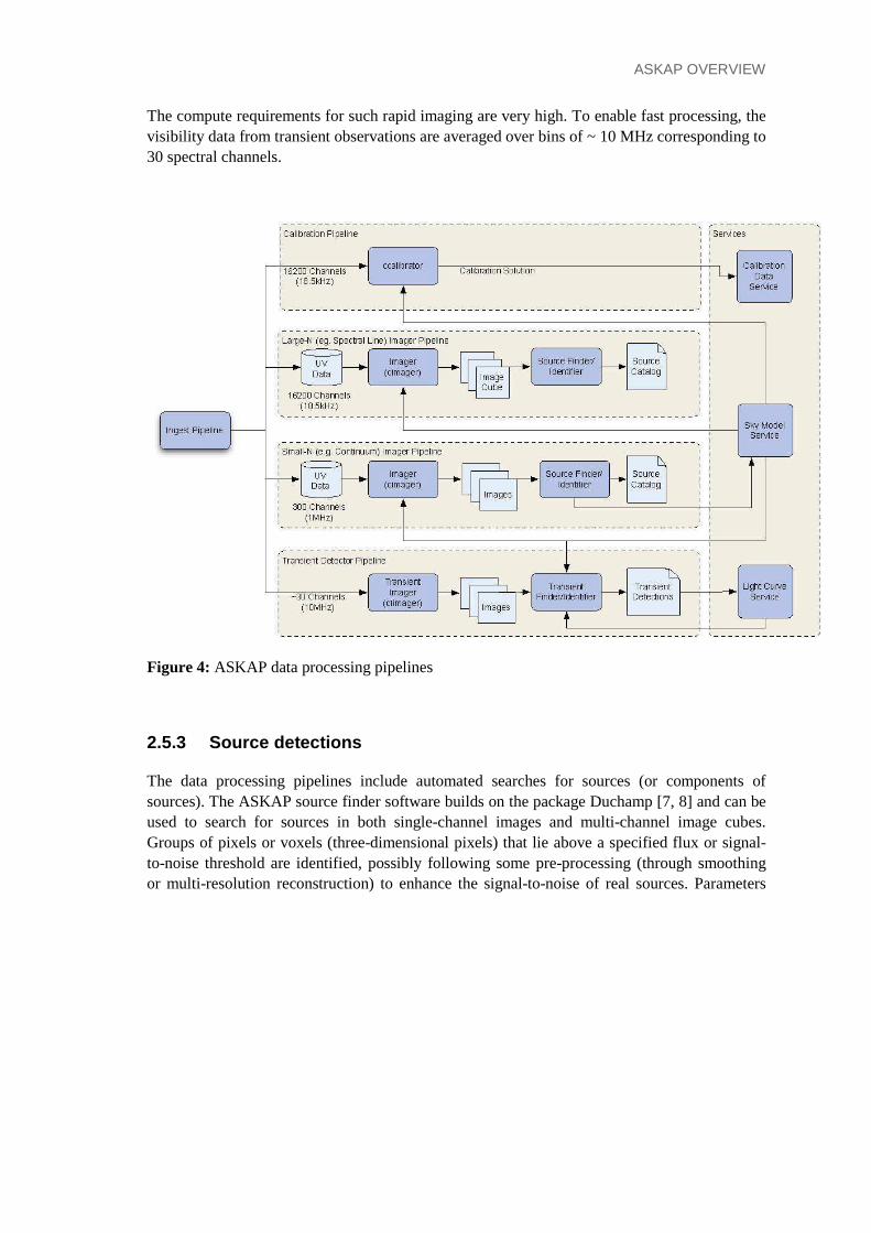
The compute requirements for such rapid imaging are very high. To enable fast processing, the visibility data from transient observations are averaged over bins of ~ 10 MHz corresponding to 30 spectral channels.
Figure 4: ASKAP data processing pipelines
2.5.3 Source detections
The data processing pipelines include automated searches for sources (or components of sources). The ASKAP source finder software builds on the package Duchamp [7, 8] and can be used to search for sources in both single-channel images and multi-channel image cubes. Groups of pixels or voxels (three-dimensional pixels) that lie above a specified flux or signal-to-noise threshold are identified, possibly following some pre-processing (through smoothing or multi-resolution reconstruction) to enhance the signal-to-noise of real sources. Parameters
ASKAP OVERVIEW
17 ASKAP-SW-0017 October 2013
characterising the source detections, such as their position on the sky, size, position angle, strength and frequency are written into source catalogues2, in effect with one source detection per catalogue row.
For transient observations, each image cube is searched and the results written into catalogues with a cadence of 5 s. The image cubes themselves are not retained. The transient catalogues allow for the construction of catalogues containing the time-dependent information needed to generate source light curves and to allow subsequent sampling or smoothing over longer time intervals. This capability will enable studies of sources that vary on timescales longer than 5 seconds.
2.5.4 Data sizes and postage stamp image cubes
In some cases the data volumes for image cubes are large. As an example, the data volume for an image cube with 3,600 x 3,600 pixels in the x- and y-directions and 16,200 spectral channels is 840 GB.
For some spectral line surveys, in addition to full-size image cubes, smaller ‘postage stamp’ image cubes will be produced with a set of smaller image cubes for a given survey field. This may be done to allow high resolution image cubes to be generated, or where source positions or velocities are known in advance. For example, a postage stamp image with 16,200 spectral channels and 128 x 128 pixels has a data volume of approximately 1 GB.
Table 2 provides some examples to illustrate data volumes for data products produced by the science data processing pipelines.
INTRODUCTION
INTRODUCTION
ERROR! NO TEXT OF SPECIFIED STYLE IN DOCUMENT.
ERROR! NO TEXT OF SPECIFIED STYLE IN DOCUMENT.
2 For this document a catalogue is conceptually equivalent to a two-dimensional table where each row contains a set of attributes for an object. For example, for a source detection catalogue each row will include the right ascension, declination, size, measured brightness and other attributes for one source.

ASKAP OVERVIEW
18 ASKAP-SW-0017 October 2013
Table 2: Example data sizes
Survey Type
Product Parameters used Output size
Notes
C Full polarisation continuum calibrated visibility data set
36 beams
300 channels
4 polarisations
666 baselines (includes auto-correlations)
Time per sample 5s
12 hours integration
2.24 TB Data volume calculated as 9 Bytes per sample = 8 Bytes per visibility + 1 Byte for weighting.
S One spectral line image cube
3,600 x 3,600 pixels
16,200 channels
1 polarisation
839 GB
S 3000 postage stamp image cubes
40 x 40 pixels
16,200 channels
1 polarisation
0.31 TB
C Set of 11 continuum images generated using ‘Taylor-term’ images
10,800 x10,800 pixels
1 channel
5.2 GB 0.47 GB per image.
Data are averaged to a single frequency channel.
11 images per field produced for multi-frequency synthesis.
C Set of 4 polarisation continuum image cubes
10,800 x 10,800 pixels
300 channels
4 polarisations
560 GB 139 GB per polarisation
S Source detections catalogue generated from one 12 hour spectral line image cube
500 detections
300 Bytes per row
150 KB Estimate only
T Bright source detections from one 5s image cube
1000 detections
300 Bytes per row.
300 KB Estimate only
ASKAP OVERVIEW
19 ASKAP-SW-0017 October 2013
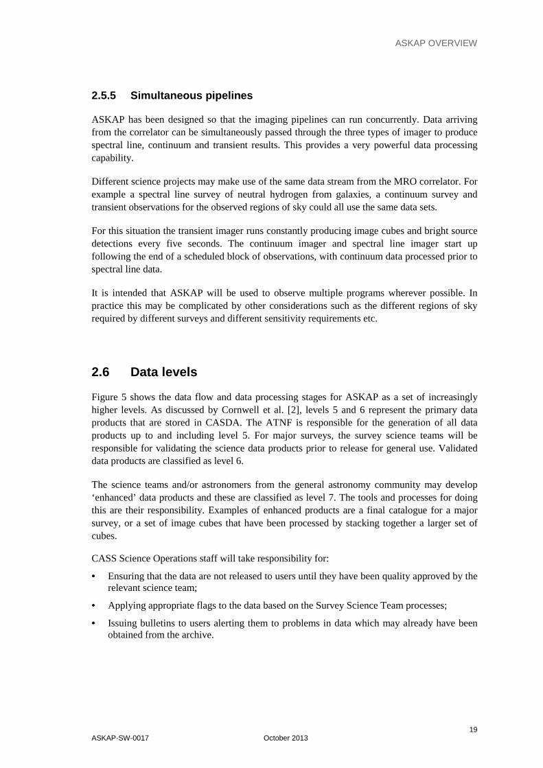
2.5.5 Simultaneous pipelines
ASKAP has been designed so that the imaging pipelines can run concurrently. Data arriving from the correlator can be simultaneously passed through the three types of imager to produce spectral line, continuum and transient results. This provides a very powerful data processing capability.
Different science projects may make use of the same data stream from the MRO correlator. For example a spectral line survey of neutral hydrogen from galaxies, a continuum survey and transient observations for the observed regions of sky could all use the same data sets.
For this situation the transient imager runs constantly producing image cubes and bright source detections every five seconds. The continuum imager and spectral line imager start up following the end of a scheduled block of observations, with continuum data processed prior to spectral line data.
It is intended that ASKAP will be used to observe multiple programs wherever possible. In practice this may be complicated by other considerations such as the different regions of sky required by different surveys and different sensitivity requirements etc.
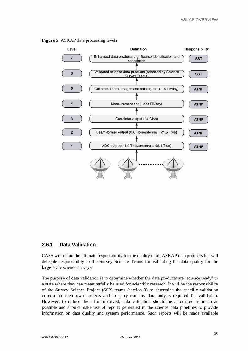
2.6 Data levels
Figure 5 shows the data flow and data processing stages for ASKAP as a set of increasingly higher levels. As discussed by Cornwell et al. [2], levels 5 and 6 represent the primary data products that are stored in CASDA. The ATNF is responsible for the generation of all data products up to and including level 5. For major surveys, the survey science teams will be responsible for validating the science data products prior to release for general use. Validated data products are classified as level 6.
The science teams and/or astronomers from the general astronomy community may develop ‘enhanced’ data products and these are classified as level 7. The tools and processes for doing this are their responsibility. Examples of enhanced products are a final catalogue for a major survey, or a set of image cubes that have been processed by stacking together a larger set of cubes.
CASS Science Operations staff will take responsibility for:
• Ensuring that the data are not released to users until they have been quality approved by the relevant science team;
• Applying appropriate flags to the data based on the Survey Science Team processes;
• Issuing bulletins to users alerting them to problems in data which may already have been obtained from the archive.
ASKAP OVERVIEW
20 ASKAP-SW-0017 October 2013
Figure 5: ASKAP data processing levels
2.6.1 Data Validation
CASS will retain the ultimate responsibility for the quality of all ASKAP data products but will delegate responsibility to the Survey Science Teams for validating the data quality for the large-scale science surveys.
The purpose of data validation is to determine whether the data products are ‘science ready’ to a state where they can meaningfully be used for scientific research. It will be the responsibility of the Survey Science Project (SSP) teams (section 3) to determine the specific validation criteria for their own projects and to carry out any data anlysis required for validation. However, to reduce the effort involved, data validation should be automated as much as possible and should make use of reports generated in the science data pipelines to provide information on data quality and system performance. Such reports will be made available
(~15 TB/day)

ASKAP OPERATIONS AND SCIENCE
21 ASKAP-SW-0017 October 2013
through CASDA. In some cases it may be necessary for science teams to retrieve visibility and or image data files from the archive for validation purposes. Where files are not archived special consideration for data access may need to be considered.
A CASDA tool will be used so that data validation metadata flags are set in the science data archive. Following validation procedures the science team will either set a survey science data quality flag that allows the data products to be released to the general community, or will flag the data as ‘bad data’. Science teams may also provide information on specific problems encountered so that this can be shared with other users. In general, observations with bad data will be repeated. However, bad data sets will not be removed from the archive as these could potentially be useful for engineering tests or other purposes.
Some administration and operations staff will also be able to set or potentially override the data validation flags. Changes to data quality flags will be tracked.
3. ASKAP OPERATIONS AND SCIENCE
3.1 ASKAP science observations
This section provides an overview of ASKAP observing and operations. For additional information see documents [1, 3, 6, 7, 8].
ASKAP will be operated by CSIRO as part of the Australia Telescope National Facility (ATNF). The ATNF also includes the Australia Telescope Compact Array, the Parkes radio telescope, and the Mopra radio telescope. These facilities are used together for Very Long Baseline Interferometry (VLBI) observations with the Long Baseline Array. All data taken on ATNF facilities belong to CSIRO.
Due to the remoteness of the MRO, ASKAP science observations will be taken in a remote-observing mode, normally from the Science Operations Centre in Marsfield, Sydney. The control and monitoring of the antennas will be carried out by CASS Science Operations staff using facilities provided by the Telescope Operating System. The science teams will not be present for the observations. Instead they will interact with the data products and information provided in CASDA.
The scientific use of ASKAP will be open to astronomers from around the world, with telescope time allocated on the basis of scientific merit and technical feasibility. ASKAP science users will include science teams who submit proposals and are allocated time for their projects, and the international general astronomical community who make use of ASKAP results through the science data archive but are not directly included on the project teams.
As a rough estimate, the number of users of ASKAP data is expected to be at least 1500 individuals. This includes approximately 350 individuals on the Survey Science Projects (section 3.3), 400 individuals on Guest Science Projects (section 3.4) and 750 individuals from the general astronomical community. The science users of ASKAP include about 30 research scientists working for CASS who participate as members of the science teams.
ASKAP OPERATIONS AND SCIENCE
22 ASKAP-SW-0017 October 2013
User support for CASDA will be provided by CASS Science Operations staff. The full user support model is not yet developed and this will be discussed in a separate document. However it is expected that general user support for using the archive will be provided by CASS staff. Such CASS support is likely to include on-line user documentation, a helpdesk-type service for enquiries, news bulletins and similar information provided through ATNF newsletters and email distributions. Community training sessions and some one-to-one support will assist users to get started with the archive.
3.2 Early Science
CASDA will provide archive support to the science observations taken from the start of Early Science. Early Science will begin following the commissioning and science verification of the first 12 MkII PAFs and is currently expected to commence about April 2015. During Early Science, observations will be classified as ‘shared risk’ and the time available at the array will be shared between commissioning activities and science use.
Planning for Early Science, led by the ASKAP Project Scientist, is now underway in consultation with the Survey Science teams. The observations will be carried out by a commissioning team on behalf of the community. Following data validation the data products will be made publically available through CASDA without a proprietary period.
The archive requirements for Early Science are essentially the same as for full ASKAP operations. However, not all observing modes will initially be available. It is expected that Early Science observing will include continuum, and spectral line observations with some initial data processing support for polarisation. Transient-mode observing will be introduced at a later time.
Some aspects of Early Science will require CASDA to be responsive to ongoing developments. Here we note that:
• At the start of Early Science, some parts of the data processing pipelines will not be fully in place. As a result members of the science teams may become involved with the data processing and generation of data products. It is expected that this will be handled by providing accounts to some science users who will work with the data files on the RTC. Once data products are ready for release they will be transferred to Lustre disks for ingestion to the science archive.
• During Early Science the data rates and the total data volumes will be lower due to a smaller number of array antennas and to the allocation of time on the array between Early Science and science verification and commissioning.
• The intention at present is to separately maintain a simpler archive that will be used for verification and commissioning. This will be managed by the CASS Science Data Processing team and is not formally a part of the CASDA project. To enable this – scheduling blocks should include metadata to identify whether they are for science use or for the commissioning archive.
ASKAP OPERATIONS AND SCIENCE
23 ASKAP-SW-0017 October 2013
3.3 Survey Science Projects
For the first five years of routine science operations with ASKAP, it is envisaged that at least 75 per cent of time will be allocated to Survey Science Projects (SSPs). These are defined as projects that require more than 1,500 hours of observing time.
Typically, observations for a SSP will be carried out over extended periods of some months with the same instrumental set up and data processing pipelines used from day-to-day. The data products from the SSPs will be released after data validation without any proprietary period. The science teams are responsible for checking and validating the primary data before they are released to the user community, and for working together with CASS to ensure that their science goals are achievable and met.
In September 2009, ten Survey Science Projects representing 363 investigators from 131 institutions in Australia and overseas were selected by an international panel. Ten ASKAP Survey Science Projects were approved:
• AS014: Evolutionary Map of the Universe (EMU)
• AS016: Widefield ASKAP L-Band Legacy All-Sky Blind Survey (WALLABY)
• AS002: The First Large Absorption Survey in HI (FLASH)
• AS004: An ASKAP Survey for Variables and Slow Transients (VAST)
• AS005: The Galactic ASKAP Spectral Line Survey (GASKAP)
• AS007: Polarization Sky Survey of the Universe's Magnetism (POSSUM)
• AS008: The Commensal Real-time ASKAP Fast Transients survey (CRAFT)
• AS012: Deep Investigations of Neutral Gas Origins (DINGO)
• AS015: Compact Objects with ASKAP: Surveys and Timing (COAST)
• AS003: The High Resolution Components of ASKAP: Meeting the Long Baseline Specifications for the SKA (VLBI)
Of the ten projects: EMU and WALLABY were assigned the highest ranking and will receive full CASS support. Six projects (DINGO, FLASH, GASKAP, POSSUM, VAST and CRAFT) were highly ranked. CASS will make all reasonable efforts to support these projects. Two projects (COAST and VLBI) were designated as strategic priorities. CASS will work to ensure that the capabilities defined by these are enabled to the extent possible.
The following notes briefly describe some of the science goals of the Survey Science Projects and some of the technical challenges associated with these projects. Further information on the Survey Science Projects is given in sections 4 and 5 and in Appendix C.
3.3.1 EMU
EMU is a deep radio continuum survey that will cover the southern sky, extending up to declination of +30 degrees. The total survey area of about 31,000 square degrees will require over 10,000 hours of telescope time and, with a full array of 36 antennas, will detect
ASKAP OPERATIONS AND SCIENCE
24 ASKAP-SW-0017 October 2013
approximately 70 million galaxies. This will be by far the most extended sensitive survey of radio sources available.
The EMU science data processing will produce catalogues of source detections. These detections will form the basis for a range of science goals that include studies of the evolution of star forming galaxies and galaxies with active nuclei (AGN), and exploring the large-scale structure of the Universe at radio wavelengths.
EMU observations will also cover our own Galaxy and will provide a sensitive wide-field atlas showing the distribution of thermal and non-thermal radio continuum sources in the Galaxy.
The EMU science team will produce a set of source catalogues including associations with catalogues of sources with results from major surveys at other wavelengths. These cross-identifications are critical in associating the detected sources with known objects and with identifying new types of sources. It is expected that several versions of the source catalogues will be produced.
3.3.2 POSSUM
The POSSUM project will study large-scale astrophysical magnetic fields. Magnetic fields are associated with many fundamental astrophysical processes. For example, magnetic fields influence the onset of star formation, mass-loss from evolved stars, the acceleration and confinement of particles in gas and the collimation of jets of matter. Such processes take place across many different scale sizes in our Galaxy as well as in other galaxies and the inter-galactic medium.
POSSUM aims to improve our understanding of magnetic fields in the Universe by studying observed polarisation properties of detected radio sources. The POSSUM data products will enable studies of magnetic field studies of our Galaxy, other galaxies and galaxy clusters, and will provide a census of magnetic fields as a function of redshift, or distance in the Universe.
The POSSUM observing strategy for ASKAP is complementary to EMU. Observations for both projects will cover the same regions of sky and it is likely that these two projects will be carried out commensally. In effect, the continuum pipeline data processor will process a single stream of visibility data arriving from the correlator to produce the images and catalogues for both projects. Whilst the EMU survey will use total intensity (STOKES I) images, the POSSUM survey will use image cubes obtained for all Stokes parameters (Stokes I, Q, U and V). From these, Faraday rotation measures will be obtained for detected sources.
The polarisation-related catalogues will include a POSSUM Polarisation Catalogue with source rotation measures and a Polarisation Atlas with frequency-dependent polarisation information.
3.3.3 WALLABY
The WALLABY survey is a ‘blind’ survey of the southern sky to search for neutral hydrogen (HI) emission from galaxies. HI is the principal component of cool gas and this can be used to

ASKAP OPERATIONS AND SCIENCE
25 ASKAP-SW-0017 October 2013
study how galaxies are formed and evolve over time and how they may merge or interact with other galaxies.
The survey aims to detect HI from around half a million galaxies with redshifts of 0 < z < 0.26, corresponding to a look back time of 3 billion years. The observations will enable studies covering distances from High Velocity Clouds associated with our own Galaxy, to the Local Group of galaxies, and beyond to more distant clusters and super clusters.
The data volumes arising from ASKAP spectral line surveys are large and some compromises are required to make the data processing and storage manageable. The full WALLABY survey will generate around 96 PB of calibrated visibility data that are then processed to form image cubes. Given this extremely large data volume, the calibrated visibility data will not be archived.
For WALLABY it is likely that two types of data cubes will be produced:
• Low spatial resolution data cubes with full spectral coverage (16,200 channels). These will be restricted to using data from baselines below 2 km. (Using a maximum baseline of 2 km instead of 6 km reduces the cube data size by a factor of nine and degrades the spatial resolution by a factor of 3.
• Postage stamp cubes with higher spatial resolution will be generated for small regions around the positions of sources detected from analysis of the full-sized cubes. For each survey field, many such postage stamp cubes may be generated.
3.3.4 DINGO
The DINGO survey will study the evolution of HI in the universe from the present time, back to a time when the universe was approximately half of its current age. The survey aims to detect HI spectral line emission from about 100,000 galaxies with redshifts of 0 < z < 0.5. Unlike WALLABY which is a ‘blind’ survey of the sky, the DINGO fields will be selected from the GAMA (Galaxy and Mass Assembly) survey.
DINGO data will be used to study cosmological ‘distribution functions’ that describe how HI is distributed in galaxies and galaxy clusters. By combining the radio data with extensive information available from the GAMA and other surveys it will be possible to study the evolution and formation of distant galaxies, and the co-evolution of the stellar, gaseous and dark matter components of galaxies.
DINGO will obtain sensitive observations of a small number of survey fields with each field observed many times. Approximately 2,500 hours will be spent observing five regions of sky. In addition a deeper search will be obtained for two fields with 2,500 hours observing time on each field.
Following each scheduling block the science data processing pipeline will produce the data cubes for each survey field and these will be processed using the source finder with results written into source detection catalogues.
ASKAP OPERATIONS AND SCIENCE
26 ASKAP-SW-0017 October 2013
The survey team will use image stacking techniques to combine the data cubes so that a single final data cube is produced for each survey region. Each of the final stacked data cubes may contain up to 10,000 galaxies. Other advanced techniques such as spectral stacking across many galaxies may also be used.
Once the final data cubes are produced, these will be made available to the general community. Stacked image cubes and the science catalogues produced by the survey science team may be released at phased intervals prior to the full completion of the survey.
3.3.5 FLASH
The FLASH project will carry out a blind survey to search for extragalactic neutral hydrogen seen in absorption. In these absorbing systems cool hydrogen gas located in a galaxy or galaxy halo absorbs radio continuum emission from a more distant background source such as a radio galaxy or quasar. The absorbing system is located along the sight line from the observer to the background source. The survey expects to detect up to 1,000 extragalactic hydrogen absorbing systems with approximately one detection per survey field. These will be used for studies of the galaxy evolution and star formation in particular for galaxies in a redshift range of 0.5 < z < 1.0.
The FLASH survey will target 850 survey fields and will identify 150,000 known continuum sources within these fields so that in effect each survey field will include around 150 to 200 sight lines to background sources. Prior to the start of the survey the Survey Science Team will generate a Target Source Catalogue that includes the positions of the continuum sources.
The data pipeline processing for FLASH will produce small postage stamp image cubes with full spectral coverage, centred on the positions of the known continuum sources The source detection process is relatively straightforward: For each survey fields a spectrum is extracted at the position of each of the continuum sources and searched for HI absorption.
3.3.6 GASKAP
The GASKAP Survey Science team will carry out several surveys of gas in our Galaxy, the Magellanic Clouds, and the regions between the Clouds (the Magellanic Bridge) and between the Clouds and our Galaxy (the Magellanic Stream). These surveys will study spectral line emission and absorption from neutral hydrogen atoms (HI) at a wavelength of 21 cm and from hydroxyl (OH) OH molecules at a wavelength of 18 cm. The surveys will provide images of extended gas emission with greater spatial resolution and coverage than has previously been achieved. They will also lead to the detections of thousands of compact sources, in most cases associated with either star formation regions or with evolved stars and supernovae.
In total GASKAP will observe around 480 fields with the observations taken over approximately 8,000 hours. Three different integration times will be used with 12.5, 50 and 200 hours per field allocated to different survey regions.
The GASKAP surveys pose some particular ASKAP challenges. In particular:

ASKAP OPERATIONS AND SCIENCE
27 ASKAP-SW-0017 October 2013
• GASKAP will require the use of ASKAP zoom modes. Standard ASKAP observations use 16,200 channels across a bandwidth of 300 MHz corresponding to a frequency resolution of around 18.5 kHz. This is too coarse a resolution for Galactic spectral line studies where a resolution of around one kHz is typically needed. To achieve the required resolution, the 16,200 channels will be used split into three narrower sub-bands to cover the HI and OH (1612 and1665/1667) transitions.
• To produce the final image cubes for the HI surveys, the ASKAP data cubes will be combined with data cubes already obtained from single dish observations. The addition of single dish data greatly improves the image quality for extended and complex structures. In principle several different techniques can be used for combining single dish and interferometric observations. Decisions on the approach to use are still to be made. At present it is not yet clear whether the HI data combination will be carried out as part of the pipeline data processing or will require post processing.
3.3.7 VAST
The VAST project will use the fast survey speed of ASKAP to investigate astrophysical objects that vary on timescales of 5 seconds or longer. Such sources span a huge range of scales, from Galactic to cosmological distances. They include flare stars, intermittent pulsars, X-ray binaries, magnetars, intra-day variables, supernovae and gamma ray bursts. Although the range of phenomena is very large, the underlying physics is generally associated with explosive events, propagation effects or by events linked to accretion and magnetism. VAST is likely to discover types of variable sources that so far are not known.
The VAST project observing strategy has two approaches:
• Where feasible, VAST will make use of ‘piggy-back’ observing where data taken for other projects is also analysed for transient sources.
• VAST will also make use of dedicated blocks of observing time. This will be used for repeated observations of target fields. A large-scale survey (VAST-wide) covering approximately 500 square degrees is planned with the entire survey region observed daily using short integrations for each survey field. A deeper survey (VAST-deep) of the same survey region but with longer integration times, and a smaller survey of the Galactic Plane may also be undertaken.
As indicated above, observations for VAST are not expected to be carried out during Early Science. The science data processing pipeline requirements for VAST are highly computing intensive with many data processing challenges to address. The ASKAP transient pipeline will be developed after the continuum and spectral line pipelines are in place and will build strongly on the experience gained.
3.3.8 COAST
The COAST Survey Science Project will use the ASKAP array to study radio emission from pulsars. These are highly compact evolved stars that rotate and emit highly beamed radio emission as a series of radio pulses. Pulsars fall into two groups – ‘standard’ pulsars with

ASKAP OPERATIONS AND SCIENCE
28 ASKAP-SW-0017 October 2013
periods of typically one second and ‘millisecond’ pulsars where the rotation rate is much faster. The time-related properties of pulsars can be measured to extremely high precision and this allows pulsars to be used as tools across a range of studies including tests of general relativity and gravitational wave studies. A key goal for pulsar astronomy is to detect gravitational waves, either from individual sources, or from a stochastic background. In addition pulsars are used to study the properties and evolution of neutron stars. Understanding their internal structures, emission mechanisms and magnetic fields remains highly challenging.
The COAST ASKAP pulsar observations will use the array in a special mode where subsets of antennas are used together in a tied-array mode. In effect each tied array acts as a single dish. The use of multiple tied arrays is anticipated as this would significantly improve the survey speed for ASKAP pulsar surveys.
The COAST planning includes two types of pulsar observations corresponding to timing and search modes:
a) Timing-mode observations of pulsars with known rotational periods. For this mode voltages at the antennas are sampled directly without using the correlator. The data are streamed off-line to another location where they are de-dispersed (to correct for dispersion and propagation effects in the interstellar medium) and ‘folded’ to the known pulsar period. By using multiple tied-array beams ASKAP will be able to observe 10s of pulsars at the same time giving it a multiplexing advantage when compared to a single dish such as Parkes. The main data products produced by timing observations are folded pulsar profiles and time series data.
b) Sensitive targeted search-mode observations will be carried out to look for pulsar emission from compact sources that are identified in other ASKAP surveys such as EMU. As for timing observations this mode takes the data stream from the MRO before it reaches the correlator. The search mode data volumes produced by timing and targeted search modes are comparable to those generated at Parkes. Data processing generates a list of pulsar candidates. These are then followed up with further observations to determine whether pulsars are present. (Table 6).
In addition, a more complex search mode may be used where the data correlator is used to produce visibility files with an extremely high data rate of 2 milliseconds per sample. This ‘fast dump visibility search’ mode requires additional custom hardware and generates high data rates (Table 6). The feasibility of this is still under discussion.
Almost all pulsar data are retained using a standard PSRFITS file format. This is compatible with VO protocols.
COAST pulsar data will NOT be processed at the Pawsey Centre as part of the standard ASKAP science data processing pipelines. Instead these data will processed off-line by the science team using specialised pulsar data reduction software.
Pulsar data obtained with the Parkes radio telescope is now provided to the community through the CSIRO pulsar Data Access Portal (DAP). For this facility the pulsar data are stored in Canberra and made accessible through a web interface. For further discussion, the CSIRO DAP may provide an additional or alternative archiving option for ASKAP pulsar data.
ASKAP OPERATIONS AND SCIENCE
29 ASKAP-SW-0017 October 2013
3.3.9 CRAFT
CRAFT is a project to search for and study fast transient sources that vary on timescales from approximately one millisecond to 5 seconds. The CRAFT project science goals are complementary to VAST and to some aspects of the COAST pulsar studies.
As an example of fast transients, a single intense burst of radio emission lasting for a few milliseconds was found by Lorimer et al. (2007) [11] in archival Parkes data. The subsequent detection of several of these so-called Lorimer bursts by Thornton et al. [12] confirm their origin as extragalactic and suggest there may be 10,000 such bursts per day over the sky. The origin of these bursts remains unclear and they have not yet been identified in any other wave band. The study of fast transient sources is expected to open up new windows in astronomy that include sources that are so far unknown but represent extreme states of matter and very strong magnetic and/or gravitational fields. Such sources may include Galactic neutron stars that emit irregular or giant pulses in addition to sources of extragalactic origin. A initial estimate of the possible detection rate for Lorimer bursts using ASKAP is one per day per 30 square degree field of view.
The large field of view of ASKAP together with the ability to determine a source position from interferometry provide very strong advantages for the study of transient sources. However, the data processing requirements are computationally expensive whilst the data handling requirements for signals sampled at intervals of 1 millisecond are also highly challenging.
It is likely that specialised hardware and software systems for CRAFT will be developed, potentially in several stages. Given the complexity of the CRAFT requirements at present there are no plans to include CRAFT during Early Science.
To enable CRAFT observations, a specialised backend may be installed at the MRO. This would sample the autocorrelations (total power) received from each antenna after beam forming at a time resolution of about 1 millisecond and a frequency resolution of 1 MHz. This backend would be used instead of the ASKAP correlator and would include sophisticated tools to process the data stream in real time, apply de-dispersion and look for fast transients. In addition to monitoring the total power, a rolling buffer may be used to retain the full voltage data streams for approximately 10 to 45 seconds (depending on the frequency). Following a potential transient detection the buffer data is used for further analysis. Other observing modes may also be considered.
The data processing for CRAFT will not make use of the ASKAP science data processing pipelines and will be the responsibility of the science team. However some CRAFT data products may be included in CASDA. The requirements for this are not yet well established.
3.3.10 VLBI
Very Long Baseline Interferometry (VLBI) is a technique used in radio astronomy where radio astronomy signals are recorded at different, widely separated locations and then brought together for correlation. The Australian Long Baseline Array (LBA) includes radio telescopes and Parkes, Mopra, Narrabri, Hobart and Ceduna together with the recent inclusion of antennas
ASKAP OPERATIONS AND SCIENCE
30 ASKAP-SW-0017 October 2013
at the MRO and in New Zealand. This array includes extremely long baselines of up to 5,500 km and this enables high resolution studies of compact objects.
The inclusion of ASKAP as a Survey Science Project is primarily as a technical demonstrator that will trial and demonstrate many of the techniques that will be required for the SKA. These include high-speed data recording and data transport networks, innovative correlation facilities and the development of new approaches to VLBI. VLBI science observations taken with ASKAP have so far made use of a single antenna equipped with a single-pixel feed. This will later be extended to include all available antennas linked together as a ‘tied array’ whilst innovative techniques such as cluster-to-cluster observing may be tried.
There are currently no plans to store VLBI data at the Pawsey Centre, or to provide user access to through CASDA. The inclusion of ASKAP antennas for VLBI observations will be managed as part of standard CASS LBA operations. Currently, ASKAP VLBI data files are written locally to data disks at the MRO and transferred to Perth for correlation with data from the other radio telescopes used. The correlated data are stored at the iVEC PBStore facility and made available to users through ftp.
3.4 Guest Science Projects
The Guest Science Projects (GSPs) are observational programs that require less than 1,500 hours of observing time to complete. Proposals for Guest Science Projects will be submitted through the Online Proposal Applications system (OPAL) and will be assessed by the Time Assignment Committee. It is expected that proposals will be requested, as for other ATNF facilities, every six months. Up to 25% of the total time available will be scheduled for GSPs, corresponding to about 750 hours of telescope time every six months. A typical time for a project may be around 100 hours, so approximately 10 GSPs are likely to scheduled in a six-month semester.
In most cases, the Guest Science Project data and data products will be released publicly into the ASKAP Science Archive without any proprietary period. However, if reasonable grounds are established in the proposal, the Time Assignment Committee will have the discretion to allow a proprietary period of up to 12 months.
The data products for the GSPs will not be validated by the science teams as these groups cannot be expected to have the level of expertise required to do this. Some data quality flags will be provided by the ASKAP hardware and science processing pipelines and these will be available to users. However the survey science data flag will be unset.
3.5 Target of Opportunity observations
These are unexpected astronomical events of extraordinary scientific interest for which observations on a short time scale are justified. Such an event might for example be a supernova explosion or the need for radio data following the detection of an unidentified burst of emission with an X-ray telescope. Observing time for Target of Opportunity is granted by the ATNF Director (who is also the CASS Chief).
ASKAP-SW-0017
Target of Opportunity observations are of immediate interest to the astronomy community. The data products will be released without any proprietary period and with minimal data validation.
4. THE SCIENCE ARCHIVE
4.1 Overview
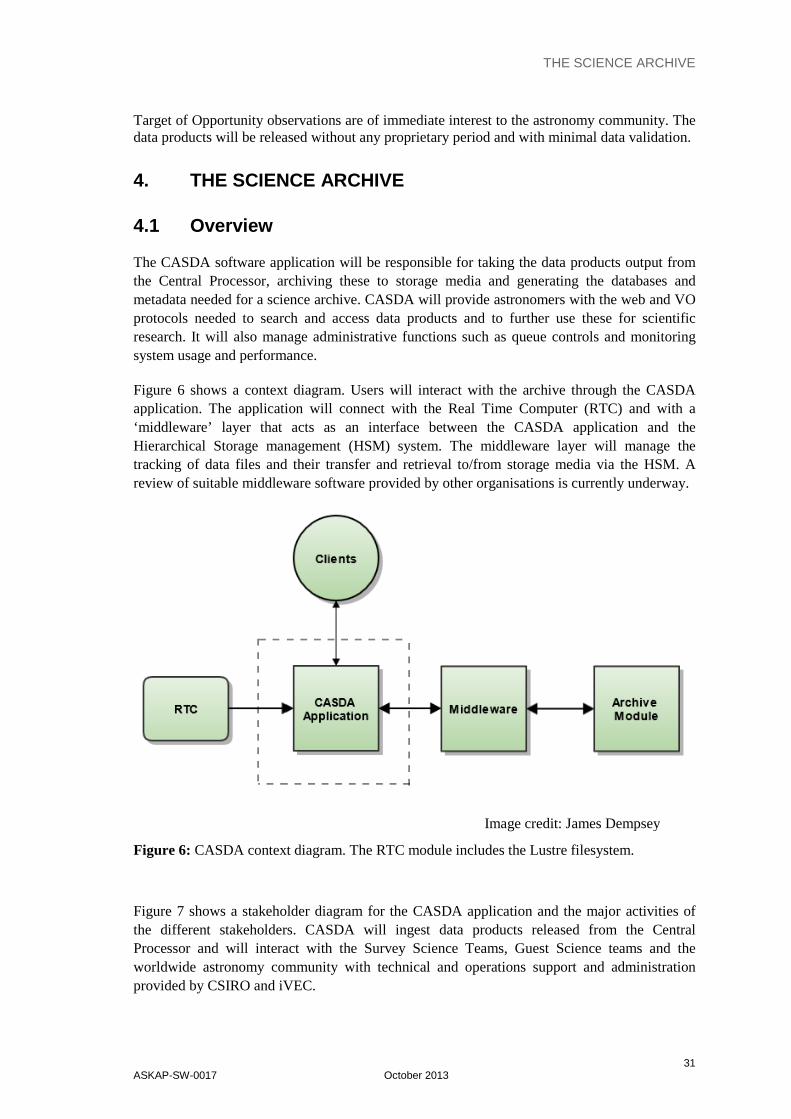
The CASDA software applthe Central Processor, archiving these to storage media and generating the databases and metadata needed for a science archive. CASDA will provide astronomers with theprotocols needed to search and access data products and to further use these for scientific research. It will also manage asystem usage and performance.
Figure 6 shows a context diagram. Uapplication. The application wil‘middleware’ layer that acts as aHierarchical Storage management (HSM) system. tracking of data files and their transfer and retrieval to/from storage mediareview of suitable middleware software provided by other organisations is currently underway.
Figure 6: CASDA context diagram. The RTC
Figure 7 shows a stakeholder diagram for the CASDA applicationthe different stakeholders. CASDA will Processor and will interact withworldwide astronomy community with provided by CSIRO and iVEC
THE SCIENCE ARCHIVE
October 2013
Opportunity observations are of immediate interest to the astronomy community. The data products will be released without any proprietary period and with minimal data validation.
THE SCIENCE ARCHIVE
The CASDA software application will be responsible for taking the data products output from the Central Processor, archiving these to storage media and generating the databases and
data needed for a science archive. CASDA will provide astronomers with theneeded to search and access data products and to further use these for scientific It will also manage administrative functions such as queue controls and monitoring
system usage and performance.
6 shows a context diagram. Users will interact with the archive through the CASDA application. The application will connect with the Real Time Computer (RTC)‘middleware’ layer that acts as an interface between the CASDA application and the Hierarchical Storage management (HSM) system. The middleware layer will manage the tracking of data files and their transfer and retrieval to/from storage mediareview of suitable middleware software provided by other organisations is currently underway.
Image credit: James Dempsey
CASDA context diagram. The RTC module includes the Lustre filesystem.
Figure 7 shows a stakeholder diagram for the CASDA application and the major actithe different stakeholders. CASDA will ingest data products released from the Central
interact with the Survey Science Teams, Guest Science teams and the astronomy community with technical and operations support and
iVEC.
THE SCIENCE ARCHIVE
31
Opportunity observations are of immediate interest to the astronomy community. The data products will be released without any proprietary period and with minimal data validation.
taking the data products output from the Central Processor, archiving these to storage media and generating the databases and
data needed for a science archive. CASDA will provide astronomers with the web and VO needed to search and access data products and to further use these for scientific
queue controls and monitoring
ract with the archive through the CASDA omputer (RTC) and with a
interface between the CASDA application and the layer will manage the
tracking of data files and their transfer and retrieval to/from storage media via the HSM. A review of suitable middleware software provided by other organisations is currently underway.
James Dempsey
includes the Lustre filesystem.
the major activities of ingest data products released from the Central
the Survey Science Teams, Guest Science teams and the support and administration

THE SCIENCE ARCHIVE
32 ASKAP-SW-0017 October 2013
Figure 7: CASDA stakeholder view
4.2 Pawsey Centre Infrastructure
CASDA will be located at the Pawsey Centre and will share infrastructure resources with other user groups. The major users of the Pawsey Centre are radio astronomy, GeoSciences, iVEC partners and users allocated resources through the National Merit Allocation Scheme. Approximately 25% of the Pawsey resources are allocated to radio astronomy to be shared between the Murchison Widefield Array (MWA) and ASKAP.
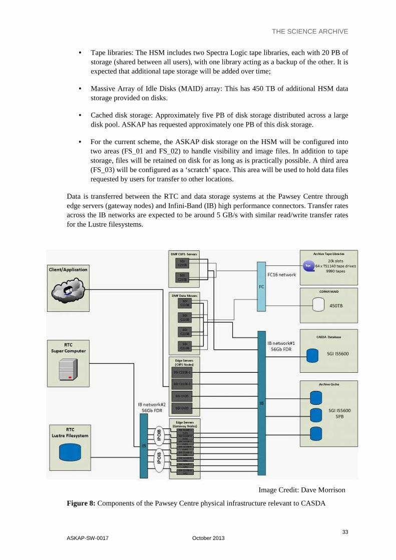
Figure 8 shows components of the physical infrastructure at the Pawsey Centre that are relevant to the science archive. The components include:
Processing platform
• RTC: This is a dedicated platform for the ASKAP Central Processor sub-system.
• Lustre Filesystem: 1.4 PB of disk space attached to the RTC is provided as scratch space for the ASKAP Central Processor.
Data products produced by the RTC are written onto the Lustre file system and transferred from there for data storage using the HSM provided by SGI.
Storage platform
THE SCIENCE ARCHIVE
33 ASKAP-SW-0017 October 2013
• Tape libraries: The HSM includes two Spectra Logic tape libraries, each with 20 PB of storage (shared between all users), with one library acting as a backup of the other. It is expected that additional tape storage will be added over time;
• Massive Array of Idle Disks (MAID) array: This has 450 TB of additional HSM data storage provided on disks.
• Cached disk storage: Approximately five PB of disk storage distributed across a large disk pool. ASKAP has requested approximately one PB of this disk storage.
• For the current scheme, the ASKAP disk storage on the HSM will be configured into two areas (FS_01 and FS_02) to handle visibility and image files. In addition to tape storage, files will be retained on disk for as long as is practically possible. A third area (FS_03) will be configured as a ‘scratch’ space. This area will be used to hold data files requested by users for transfer to other locations.
Data is transferred between the RTC and data storage systems at the Pawsey Centre through edge servers (gateway nodes) and Infini-Band (IB) high performance connectors. Transfer rates across the IB networks are expected to be around 5 GB/s with similar read/write transfer rates for the Lustre filesystems.
Image Credit: Dave Morrison
Figure 8: Components of the Pawsey Centre physical infrastructure relevant to CASDA

THE SCIENCE ARCHIVE
34 ASKAP-SW-0017 October 2013
4.3 Primary data products
Table 3 lists the ‘primary’ data products that will be produced by the science data processing pipeline and made available to users through the science archive.
As an extension to previous requirement statements, CASDA may provide tools so that the Science Survey Project teams can load VO compatible science survey catalogues, with access provided to users through CASDA and metadata to establish the ownership and provenance of such data products. By making these available to the worldwide astronomical community, the association of these science catalogues with ASKAP (and CSIRO) will be much stronger than would otherwise be the case, whilst the science benefits obtained from using the archives will be significantly increased.
The FITS format used by ASKAP will be compatible with international FITS standard. (The FITS standard is available at http://fits.gsfc.nasa.gov/fits_standard.html.) Note that other data formats are being considered for use with radio astronomy and it is possible that archive support additional or alternative data formats may be required in the future.
Table 3: CASDA data products
Ref Survey Types
Data Product Format
P1 C Calibrated continuum visibility data CASA measurement set
P2 C Continuum images and image cubes (including cut-outs)
FITS
P3 S Spectral line image cubes (including cut-outs) FITS
P4 S Spectral line postage stamp image cubes FITS
P5 S Moment maps generated from cubes FITS
P6 S Spectra extracted from cubes FITS
P7 All Calibration and system information Catalogue
P8 All Scheduling and schedule block information Catalogue
P9 All Global Sky Model
(updated in archive ~ after each scheduling block)
Catalogue
P10 All Image quality reports Catalogue
P11 C Continuum source detection catalogues Catalogue
P12 C Polarisation-related catalogues Catalogue
P13 S Spectral line source detection catalogues Catalogue
P14 T Transient source detection catalogues Catalogue
P15 All Survey Science Teams: Level 7 source catalogues
To be confirmed
Catalogue

THE SCIENCE ARCHIVE
35 ASKAP-SW-0017 October 2013
Note: Table 3 does not include the data products for VLBI, COAST and CRAFT where the data processing is handled outside of the Pawsey Centre. These are discussed in section 4.5.
4.4 Virtual Observatory protocols
We anticipate that science users of the archive will gain access to images, image cubes and catalogues using Virtual Observatory protocols. VO protocols are unlikely to be used to provide direct access to visibility data files.
The International Virtual Observatory Alliance (IVOA) provides a set of standard and internationally recognised protocols that allows users to search and access data, including images and image cubes, catalogues and derived products. The current VO protocols include:
Cone Search Protocol: This is used to search a catalogue for information corresponding to a region of sky around a specified position. The protocol uses three arguments for right ascension, declination and search radius. In response, the server sends a VO table with the results (other formats can be requested). Cone searches are commonly used in astronomy and are likely to be the most frequent search mode carried out by general users.
Simple Image Access Protocol (SIAP) This enables searches around a specified sky position and is used to find and access images and image cubes. The service can generate cut-out sections of images or cubes with user-specified dimensions. It returns a link to the requested outputs.
Simple Spectral Access Protocol: Allows for queries to return source spectra from an image or image cube.
Table Access Protocol (TAP): Allows for the construction of more complex queries of catalogues. Queries can be expressed in several ways: The result of a TAP query is generally returned as another VO table.
Note that additional VO protocols may be developed for radio astronomy, by CASS and/or other organisations and later considered for use with CASDA.
4.5 Data volumes
Table 4 summarises the data volumes for seven Survey Science Projects [2] where the data products are obtained from pipeline data processing at the Pawsey Centre. For each project the last three columns give the estimated total visibility, image-related and catalogue data volumes for the science archive based on indicative parameters. For assumptions used, detailed calculations and notes see Appendix C.
Note that the data volumes given in this table are NOT adjusted for commensal observing. However, commensal observing will reduce the total data requirements through sharing of data between projects. For example, EMU and POSSUM may use the same set of visibility data, whilst POSSUM will make use of the EMU Stokes-I images and catalogue information.

THE SCIENCE ARCHIVE
36 ASKAP-SW-0017 October 2013
Table 4: Data volumes for seven Survey Science Projects
Survey Type N
survey fields
Total time per field
Visibility data size per field
Image data size per field
(all images or image
cubes)
Total visibility
data volume
Total image / image cube data
volume
Total tables data
volume
Unit h TB TB PB PB GB
EMU C 1200 12 2.4 2.68E-3 2.8 3.2E-3 25
POSSUM C 1200 8 1.5 1.0 1.8 1.2 25
WALLABY S 1200 8 not
archived 1.8
not
archived 2.1 <1
DINGO
Deep S 5 500
not
archived 1.3
not
archived 1.3 <1
DINGO
Ultradeep S 2 2500
FLASH S 850 4 not
archived 0.48
not
archived 0.5 <1
GASKAP S 644 12.5 not
archived 1.3
not
archived 0.9 <1
VAST T 1200 12 0.224 7.0 0.27
Most
image
cubes are
not
archived
See
App B
Notes:
a) Parameters are determined using information in [2]
b) The number of fields that can be observed per day for a given project will depend on a number of factors such as the rise and set times of the regions to be observed, the location of the sun and whether projects are observed commensally with each other.

THE SCIENCE ARCHIVE
37 ASKAP-SW-0017 October 2013
Table 5 provides an estimate of data volumes for the three projects where the data are not processed through the data processing pipelines. For COAST values are given separately for different observing modes. In this table, column three gives an estimate of the data volume generated after 12 hours. Column four gives the estimated data volume for the full project.
Table 5: Survey Science Projects data volumes for COAST, CRAFT and VLBI
Survey Type
Data volume per 12 hours (GB)
Total data
volume for full project
(TB)
Notes CASDA archive
required?
COAST
(a) T 12 2.0
Timing of millisecond pulsars. Data volume after de-dispersion
and folding.
Assumes single beam.
Possibly see 3.3.8
COAST
(b) T 20 1.0
Timing of non-millisecond pulsars. Data volume after de-
dispersion and folding.
Assumes 20 tied beams
Possibly see 3.3.8
COAST
(c) T 2,000 333
Search mode for targeted sources.
Data volume for raw data
Possibly see 3.3.8
COAST
(d) T 85,000 88,000
Fast-dump visibility search mode observations.
Data volume for raw data
No
CRAFT
(e) T 1,300 1,500
Not established whether visibility data will be archived.
Some transient-related information is likely to be
archived.
Yes
VLBI C,S 50 15
Correlated visibility files are currently stored using PBStore
in Perth. These will also be included in the ATOA.
No
Notes: a) Assumes 2,000 hours for timing of millisecond pulsars. Total time assume that data are
taken over a five year period. Data volumes are rough estimates only.
b) Assumes 250 hours for timing of non-millisecond pulsars.
c) Assumes 2,000 hours for targeted search mode observations.
d) Assumes 1,250 hours for fast dump search observations taken over five years. Raw data are likely to be discarded after processing for candidate detections.
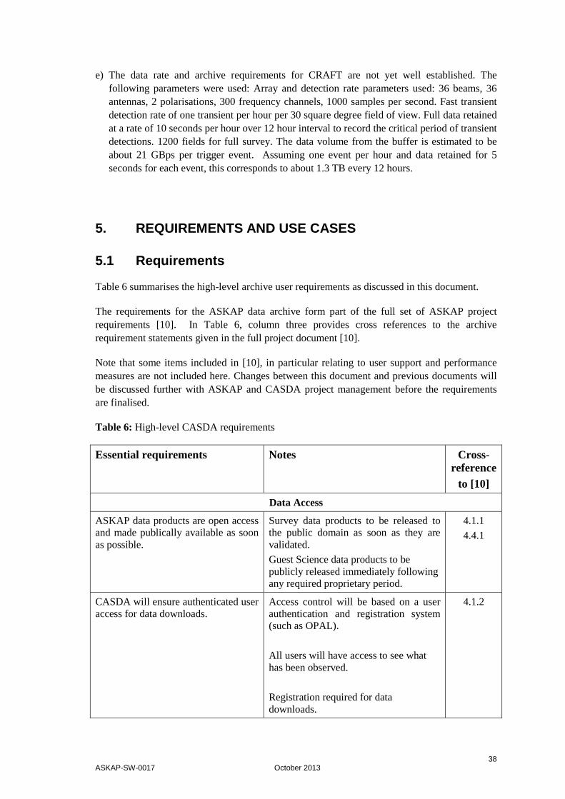
38 ASKAP-SW-0017 October 2013
e) The data rate and archive requirements for CRAFT are not yet well established. The following parameters were used: Array and detection rate parameters used: 36 beams, 36 antennas, 2 polarisations, 300 frequency channels, 1000 samples per second. Fast transient detection rate of one transient per hour per 30 square degree field of view. Full data retained at a rate of 10 seconds per hour over 12 hour interval to record the critical period of transient detections. 1200 fields for full survey. The data volume from the buffer is estimated to be about 21 GBps per trigger event. Assuming one event per hour and data retained for 5 seconds for each event, this corresponds to about 1.3 TB every 12 hours.
5. REQUIREMENTS AND USE CASES
5.1 Requirements
Table 6 summarises the high-level archive user requirements as discussed in this document.
The requirements for the ASKAP data archive form part of the full set of ASKAP project requirements [10]. In Table 6, column three provides cross references to the archive requirement statements given in the full project document [10].
Note that some items included in [10], in particular relating to user support and performance measures are not included here. Changes between this document and previous documents will be discussed further with ASKAP and CASDA project management before the requirements are finalised.
Table 6: High-level CASDA requirements
Essential requirements Notes Cross-reference
to [10]
Data Access
ASKAP data products are open access and made publically available as soon as possible.
Survey data products to be released to the public domain as soon as they are validated.
Guest Science data products to be publicly released immediately following any required proprietary period.
4.1.1
4.4.1
CASDA will ensure authenticated user access for data downloads.
Access control will be based on a user authentication and registration system (such as OPAL).
All users will have access to see what has been observed.
Registration required for data downloads.
4.1.2
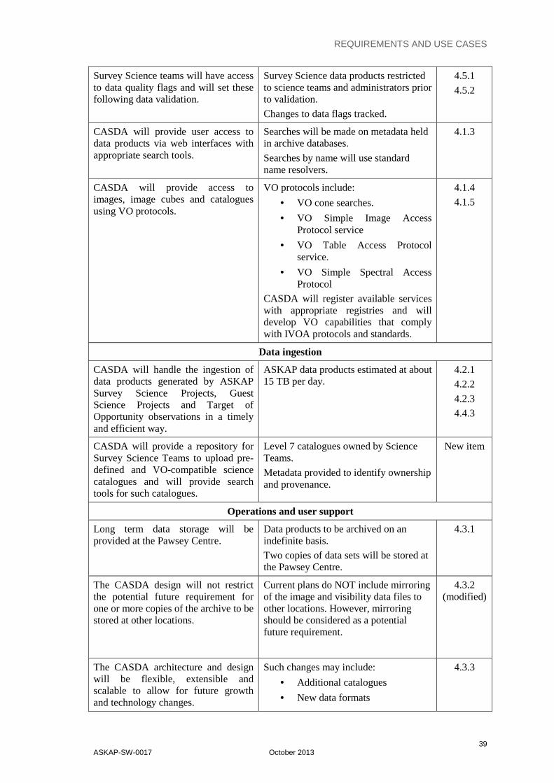
REQUIREMENTS AND USE CASES
39 ASKAP-SW-0017 October 2013
Survey Science teams will have access to data quality flags and will set these following data validation.
Survey Science data products restricted to science teams and administrators prior to validation.
Changes to data flags tracked.
4.5.1
4.5.2
CASDA will provide user access to data products via web interfaces with appropriate search tools.
Searches will be made on metadata held in archive databases.
Searches by name will use standard name resolvers.
4.1.3
CASDA will provide access to images, image cubes and catalogues using VO protocols.
VO protocols include:
• VO cone searches.
• VO Simple Image Access Protocol service
• VO Table Access Protocol service.
• VO Simple Spectral Access Protocol
CASDA will register available services with appropriate registries and will develop VO capabilities that comply with IVOA protocols and standards.
4.1.4
4.1.5
Data ingestion
CASDA will handle the ingestion of data products generated by ASKAP Survey Science Projects, Guest Science Projects and Target of Opportunity observations in a timely and efficient way.
ASKAP data products estimated at about 15 TB per day.
4.2.1
4.2.2
4.2.3
4.4.3
CASDA will provide a repository for Survey Science Teams to upload pre-defined and VO-compatible science catalogues and will provide search tools for such catalogues.
Level 7 catalogues owned by Science Teams.
Metadata provided to identify ownership and provenance.
New item
Operations and user support
Long term data storage will be provided at the Pawsey Centre.
Data products to be archived on an indefinite basis.
Two copies of data sets will be stored at the Pawsey Centre.
4.3.1
The CASDA design will not restrict the potential future requirement for one or more copies of the archive to be stored at other locations.
Current plans do NOT include mirroring of the image and visibility data files to other locations. However, mirroring should be considered as a potential future requirement.
4.3.2 (modified)
The CASDA architecture and design will be flexible, extensible and scalable to allow for future growth and technology changes.
Such changes may include:
• Additional catalogues
• New data formats
4.3.3
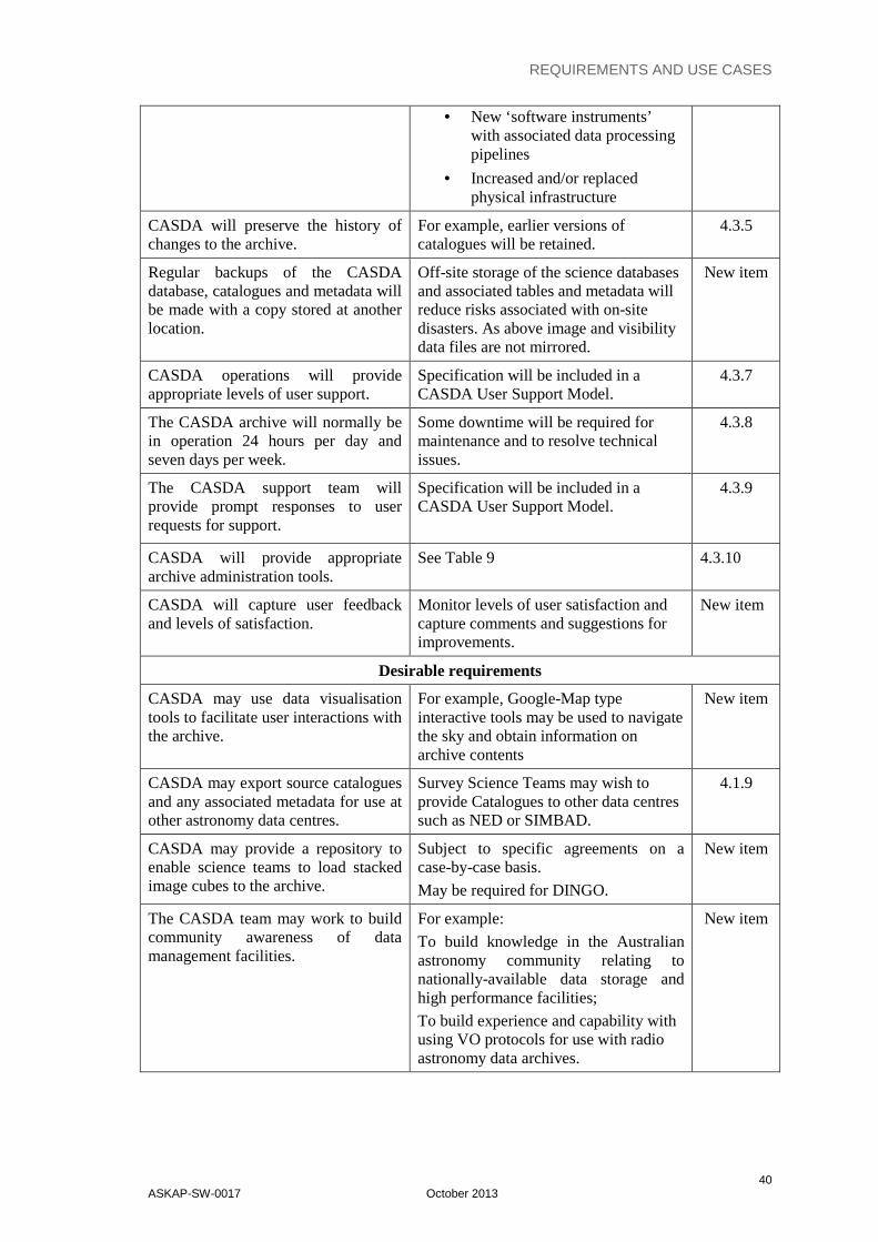
REQUIREMENTS AND USE CASES
40 ASKAP-SW-0017 October 2013
• New ‘software instruments’ with associated data processing pipelines
• Increased and/or replaced physical infrastructure
CASDA will preserve the history of changes to the archive.
For example, earlier versions of catalogues will be retained.
4.3.5
Regular backups of the CASDA database, catalogues and metadata will be made with a copy stored at another location.
Off-site storage of the science databases and associated tables and metadata will reduce risks associated with on-site disasters. As above image and visibility data files are not mirrored.
New item
CASDA operations will provide appropriate levels of user support.
Specification will be included in a CASDA User Support Model.
4.3.7
The CASDA archive will normally be in operation 24 hours per day and seven days per week.
Some downtime will be required for maintenance and to resolve technical issues.
4.3.8
The CASDA support team will provide prompt responses to user requests for support.
Specification will be included in a CASDA User Support Model.
4.3.9
CASDA will provide appropriate archive administration tools.
See Table 9 4.3.10
CASDA will capture user feedback and levels of satisfaction.
Monitor levels of user satisfaction and capture comments and suggestions for improvements.
New item
Desirable requirements
CASDA may use data visualisation tools to facilitate user interactions with the archive.
For example, Google-Map type interactive tools may be used to navigate the sky and obtain information on archive contents
New item
CASDA may export source catalogues and any associated metadata for use at other astronomy data centres.
Survey Science Teams may wish to provide Catalogues to other data centres such as NED or SIMBAD.
4.1.9
CASDA may provide a repository to enable science teams to load stacked image cubes to the archive.
Subject to specific agreements on a case-by-case basis.
May be required for DINGO.
New item
The CASDA team may work to build community awareness of data management facilities.
For example:
To build knowledge in the Australian astronomy community relating to nationally-available data storage and high performance facilities;
To build experience and capability with using VO protocols for use with radio astronomy data archives.
New item
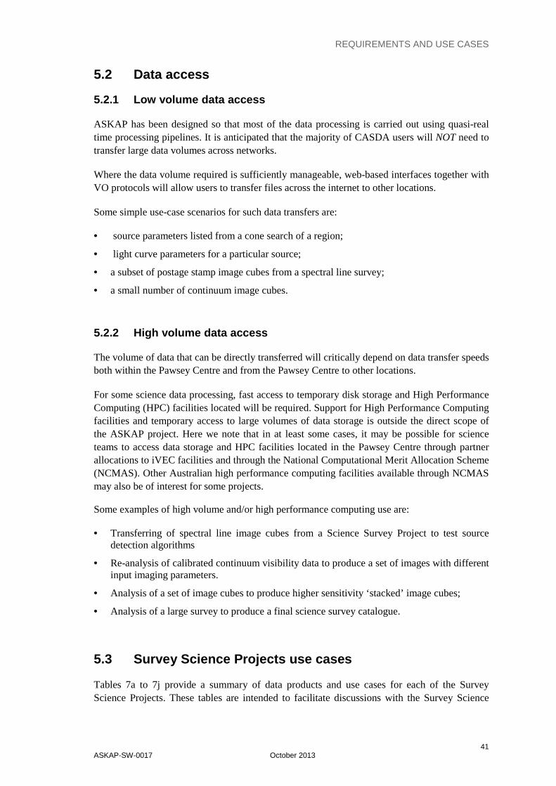
REQUIREMENTS AND USE CASES
41 ASKAP-SW-0017 October 2013
5.2 Data access
5.2.1 Low volume data access
ASKAP has been designed so that most of the data processing is carried out using quasi-real time processing pipelines. It is anticipated that the majority of CASDA users will NOT need to transfer large data volumes across networks.
Where the data volume required is sufficiently manageable, web-based interfaces together with VO protocols will allow users to transfer files across the internet to other locations.
Some simple use-case scenarios for such data transfers are:
• source parameters listed from a cone search of a region;
• light curve parameters for a particular source;
• a subset of postage stamp image cubes from a spectral line survey;
• a small number of continuum image cubes.
5.2.2 High volume data access
The volume of data that can be directly transferred will critically depend on data transfer speeds both within the Pawsey Centre and from the Pawsey Centre to other locations.
For some science data processing, fast access to temporary disk storage and High Performance Computing (HPC) facilities located will be required. Support for High Performance Computing facilities and temporary access to large volumes of data storage is outside the direct scope of the ASKAP project. Here we note that in at least some cases, it may be possible for science teams to access data storage and HPC facilities located in the Pawsey Centre through partner allocations to iVEC facilities and through the National Computational Merit Allocation Scheme (NCMAS). Other Australian high performance computing facilities available through NCMAS may also be of interest for some projects.
Some examples of high volume and/or high performance computing use are:
• Transferring of spectral line image cubes from a Science Survey Project to test source detection algorithms
• Re-analysis of calibrated continuum visibility data to produce a set of images with different input imaging parameters.
• Analysis of a set of image cubes to produce higher sensitivity ‘stacked’ image cubes;
• Analysis of a large survey to produce a final science survey catalogue.
5.3 Survey Science Projects use cases
Tables 7a to 7j provide a summary of data products and use cases for each of the Survey Science Projects. These tables are intended to facilitate discussions with the Survey Science
REQUIREMENTS AND USE CASES
42 ASKAP-SW-0017 October 2013
teams and so that each project team can verify their own set of use cases and data products with the CASDA team. The information given will be refined following feedback on this document.
Each table lists the level 5/6 data products where these are generated in the ASKAP science data processing pipelines and level 7 data products that may be generated by the science teams. A preliminary set of use cases for CASDA is also given together with some notes on data validation where this can be given. For all tables, support for items in italics are considered to be outside the scope of the CASDA project.
There is considerable overlap between the data products and use cases for the different Survey Science projects. Table 8 provides a ‘merged’ summary of use cases for science users.

REQUIREMENTS AND USE CASES
43 ASKAP-SW-0017 October 2013
Table 7a: EMU
Science Team
PI: R. Norris (CASS)
Team includes ~ 100 individuals from 13 countries
Level 5/6 data products
• Full-polarisation calibrated visibility data
• Images and image cubes are stored for Stokes I only. Images and cubes are produced for each integration block of 12 hours. Images correspond to the restored, residual and model images for each of three Taylor terms corresponding to the source intensity, spectral index and spectral curvature. An image cube will be generated for the sensitivity and another may be generated for the PSF.
• Source detection catalogue. The full survey is expected to result in approximately 70 million source detections.
Level 7 data products
• Source catalogues. Several catalogues will be produced with the release of new versions as additional or updated information becomes available. Catalogues will include associations with known sources from other major surveys.
• Stacked images The EMU team may investigate using image stacking techniques to increase the survey sensitivity.
Use cases: VO services used wherever possible
• Access summary information on observation blocks completed including information on system performance and RFI etc.
• Access information on status of tasks submitted for processing at Pawsey Centre • Access help from archive support staff • Query catalog(s) for a summary of visibility files archived and sky regions observed • Access visibility files if needed (expected to be infrequent). • Access catalogue information on image quality • Set data validation flags following review of data validation report. • Access and transfer survey images or parts of images for data validation or post
processing • Access and transfer information from source detection catalogues • Access and transfer full source detection catalogues for post-processing • Load source catalogues (level 7) into archive and allow general user access • Add new versions of source catalogues to archive, and retain previous versions • Search all source catalogues • Obtain access, as needed, to high-bandwidth and high performance computing for post-
processing including cross-identifications with other major surveys, and image stacking.
Data validation notes
The science team expect to largely use automated statistical reports provided through the archive. However it may be necessary to access some data products for closer analysis.
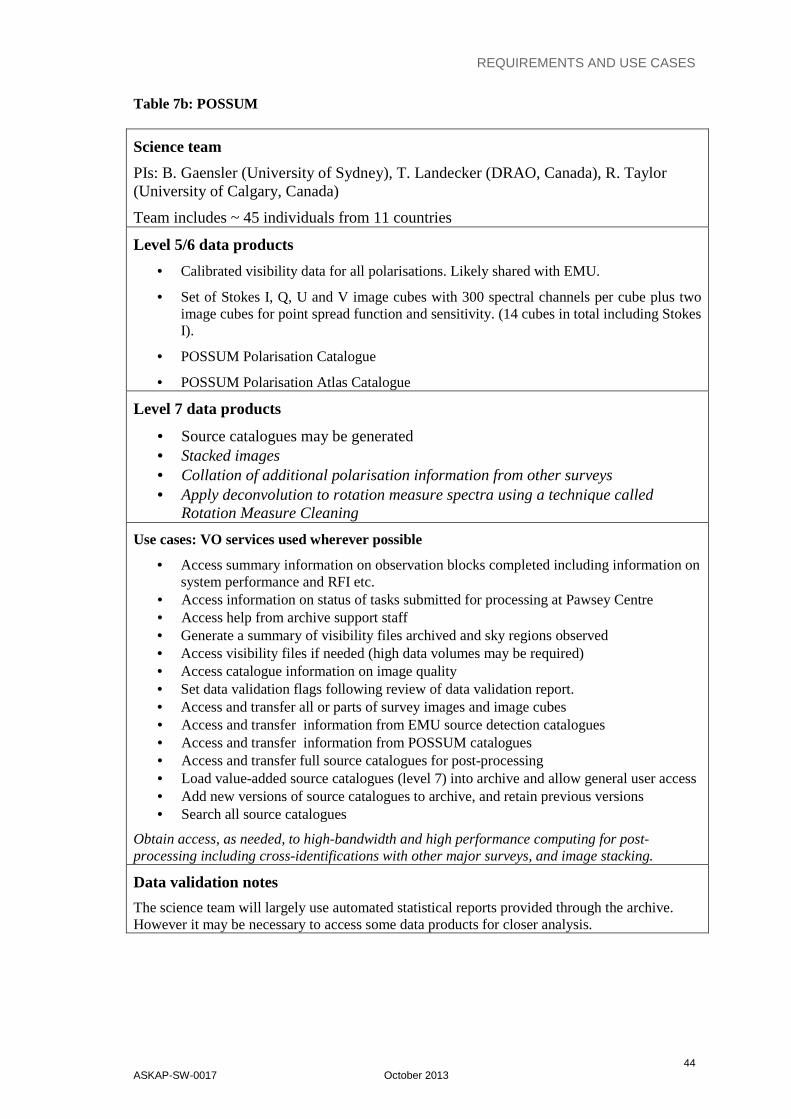
REQUIREMENTS AND USE CASES
44 ASKAP-SW-0017 October 2013
Table 7b: POSSUM
Science team
PIs: B. Gaensler (University of Sydney), T. Landecker (DRAO, Canada), R. Taylor (University of Calgary, Canada)
Team includes ~ 45 individuals from 11 countries
Level 5/6 data products
• Calibrated visibility data for all polarisations. Likely shared with EMU.
• Set of Stokes I, Q, U and V image cubes with 300 spectral channels per cube plus two image cubes for point spread function and sensitivity. (14 cubes in total including Stokes I).
• POSSUM Polarisation Catalogue
• POSSUM Polarisation Atlas Catalogue
Level 7 data products
• Source catalogues may be generated • Stacked images • Collation of additional polarisation information from other surveys • Apply deconvolution to rotation measure spectra using a technique called
Rotation Measure Cleaning
Use cases: VO services used wherever possible
• Access summary information on observation blocks completed including information on system performance and RFI etc.
• Access information on status of tasks submitted for processing at Pawsey Centre • Access help from archive support staff • Generate a summary of visibility files archived and sky regions observed • Access visibility files if needed (high data volumes may be required) • Access catalogue information on image quality • Set data validation flags following review of data validation report. • Access and transfer all or parts of survey images and image cubes • Access and transfer information from EMU source detection catalogues • Access and transfer information from POSSUM catalogues • Access and transfer full source catalogues for post-processing • Load value-added source catalogues (level 7) into archive and allow general user access • Add new versions of source catalogues to archive, and retain previous versions • Search all source catalogues
Obtain access, as needed, to high-bandwidth and high performance computing for post-processing including cross-identifications with other major surveys, and image stacking.
Data validation notes
The science team will largely use automated statistical reports provided through the archive. However it may be necessary to access some data products for closer analysis.
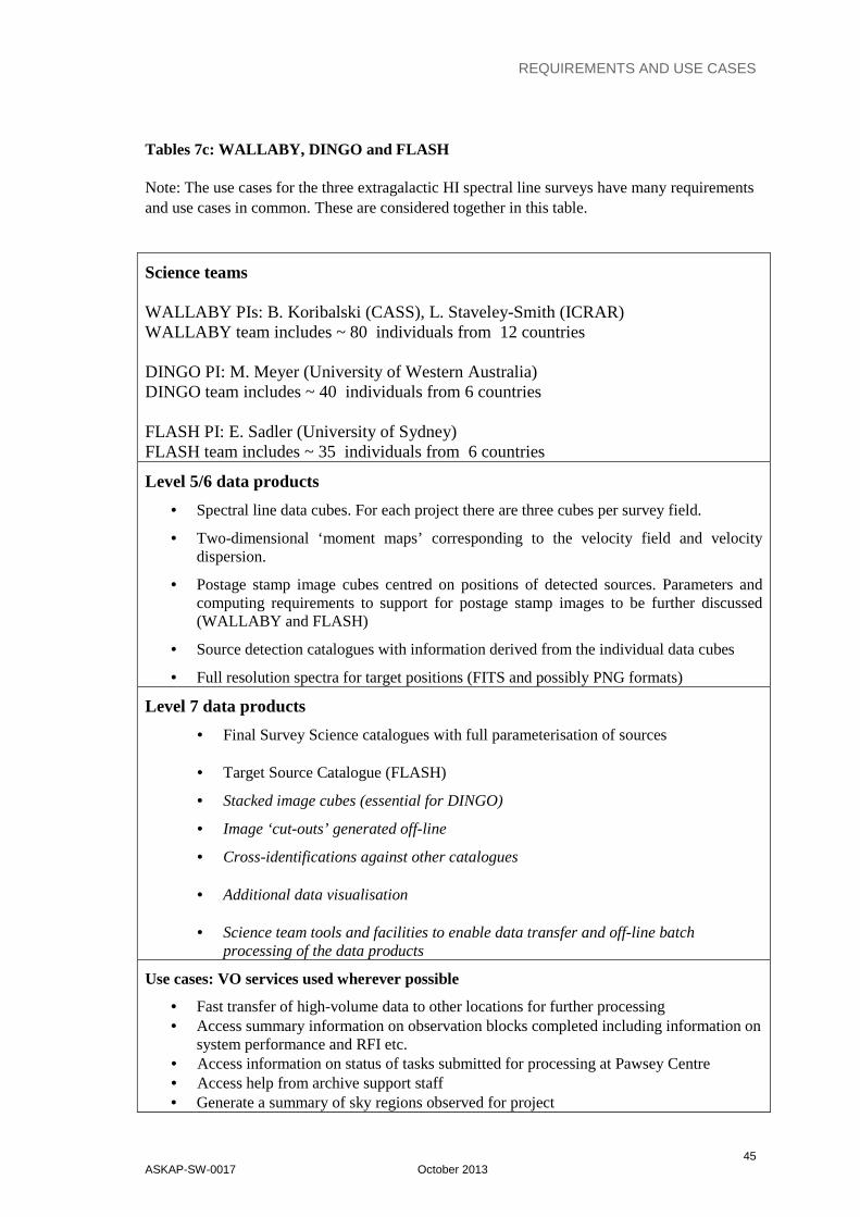
REQUIREMENTS AND USE CASES
45 ASKAP-SW-0017 October 2013
Tables 7c: WALLABY, DINGO and FLASH Note: The use cases for the three extragalactic HI spectral line surveys have many requirements and use cases in common. These are considered together in this table.
Science teams WALLABY PIs: B. Koribalski (CASS), L. Staveley-Smith (ICRAR) WALLABY team includes ~ 80 individuals from 12 countries DINGO PI: M. Meyer (University of Western Australia) DINGO team includes ~ 40 individuals from 6 countries FLASH PI: E. Sadler (University of Sydney) FLASH team includes ~ 35 individuals from 6 countries
Level 5/6 data products
• Spectral line data cubes. For each project there are three cubes per survey field.
• Two-dimensional ‘moment maps’ corresponding to the velocity field and velocity dispersion.
• Postage stamp image cubes centred on positions of detected sources. Parameters and computing requirements to support for postage stamp images to be further discussed (WALLABY and FLASH)
• Source detection catalogues with information derived from the individual data cubes
• Full resolution spectra for target positions (FITS and possibly PNG formats)
Level 7 data products
• Final Survey Science catalogues with full parameterisation of sources
• Target Source Catalogue (FLASH)
• Stacked image cubes (essential for DINGO)
• Image ‘cut-outs’ generated off-line
• Cross-identifications against other catalogues
• Additional data visualisation • Science team tools and facilities to enable data transfer and off-line batch
processing of the data products
Use cases: VO services used wherever possible
• Fast transfer of high-volume data to other locations for further processing • Access summary information on observation blocks completed including information on
system performance and RFI etc. • Access information on status of tasks submitted for processing at Pawsey Centre • Access help from archive support staff • Generate a summary of sky regions observed for project

REQUIREMENTS AND USE CASES
46 ASKAP-SW-0017 October 2013
• Access catalogue information on image quality • Set data validation flags • Access and transfer all or parts of data cubes • Access moment maps • Access and transfer HI spectra for set of sky positions • Access and transfer information from EMU source detection catalogues • Access and transfer source catalogues for post-processing • Load stacked image data cubes (in particular from DINGO) • Generate ‘cut-out’ cubelets for detected sources from data cubes in archive • Load value-added source catalogues (level 7) into archive and allow general user access • Update science catalogues • Search all source catalogues
• Access to data storage and high performance computing for off-line data processing. • Access to source finding software for external use • Combine spectral line image cubes using stacking techniques. • Generate cut-out cubelets from stacked cubes • Run source finder on stacked images.
Data validation notes
Data validation should largely use automated statistical reports provided through the archive. Calibrated visibility data files for spectral line data are not archived. However, some access to visibility data for a period of some days for validation purposes may be required. It may be necessary also to access some image data products for closer analysis.
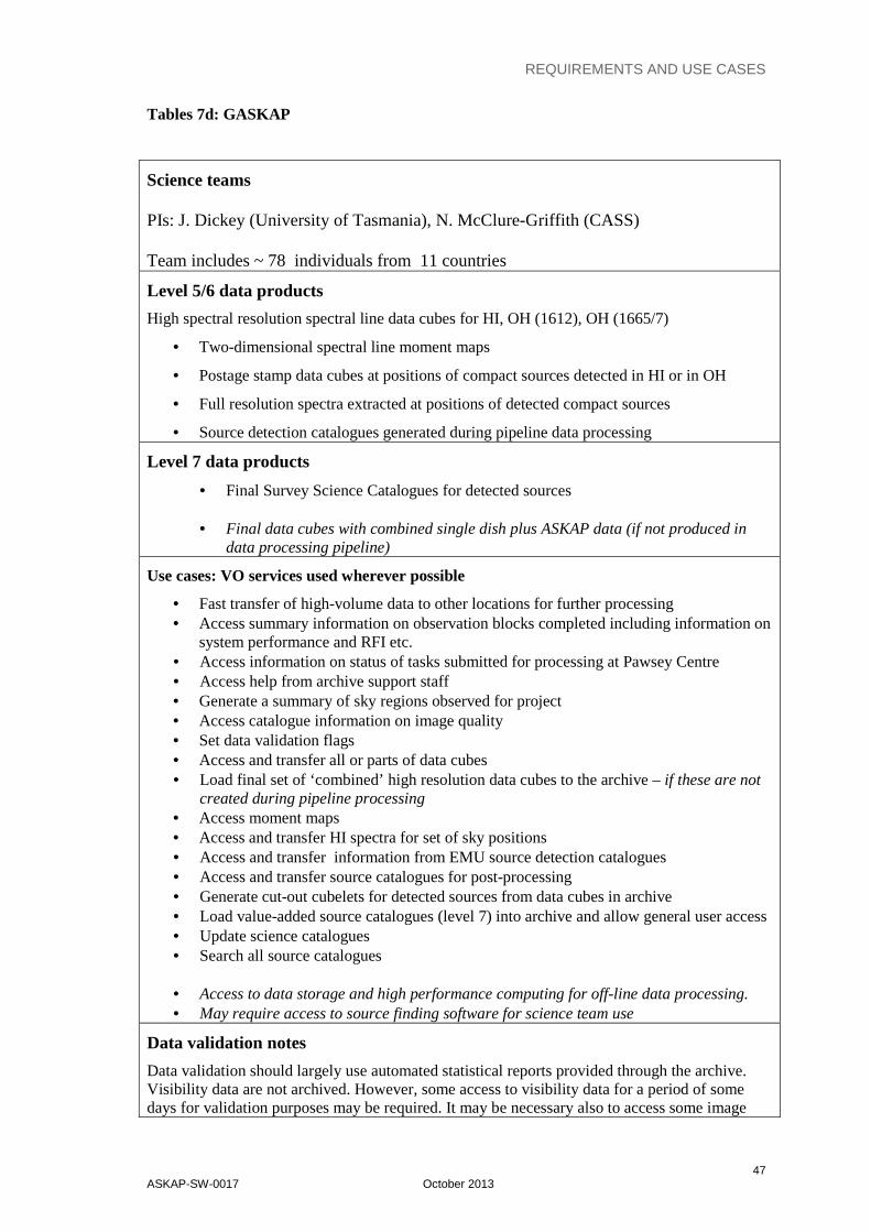
REQUIREMENTS AND USE CASES
47 ASKAP-SW-0017 October 2013
Tables 7d: GASKAP
Science teams PIs: J. Dickey (University of Tasmania), N. McClure-Griffith (CASS) Team includes ~ 78 individuals from 11 countries
Level 5/6 data products
High spectral resolution spectral line data cubes for HI, OH (1612), OH (1665/7)
• Two-dimensional spectral line moment maps
• Postage stamp data cubes at positions of compact sources detected in HI or in OH
• Full resolution spectra extracted at positions of detected compact sources
• Source detection catalogues generated during pipeline data processing
Level 7 data products
• Final Survey Science Catalogues for detected sources
• Final data cubes with combined single dish plus ASKAP data (if not produced in data processing pipeline)
Use cases: VO services used wherever possible
• Fast transfer of high-volume data to other locations for further processing • Access summary information on observation blocks completed including information on
system performance and RFI etc. • Access information on status of tasks submitted for processing at Pawsey Centre • Access help from archive support staff • Generate a summary of sky regions observed for project • Access catalogue information on image quality • Set data validation flags • Access and transfer all or parts of data cubes • Load final set of ‘combined’ high resolution data cubes to the archive – if these are not
created during pipeline processing • Access moment maps • Access and transfer HI spectra for set of sky positions • Access and transfer information from EMU source detection catalogues • Access and transfer source catalogues for post-processing • Generate cut-out cubelets for detected sources from data cubes in archive • Load value-added source catalogues (level 7) into archive and allow general user access • Update science catalogues • Search all source catalogues
• Access to data storage and high performance computing for off-line data processing. • May require access to source finding software for science team use
Data validation notes
Data validation should largely use automated statistical reports provided through the archive. Visibility data are not archived. However, some access to visibility data for a period of some days for validation purposes may be required. It may be necessary also to access some image

REQUIREMENTS AND USE CASES
48 ASKAP-SW-0017 October 2013
data products for closer analysis.
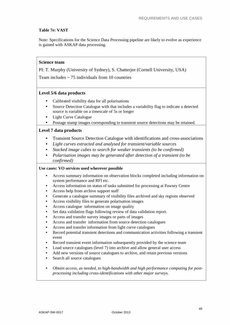
REQUIREMENTS AND USE CASES
49 ASKAP-SW-0017 October 2013
Table 7e: VAST Note: Specifications for the Science Data Processing pipeline are likely to evolve as experience is gained with ASKAP data processing.
Science team
PI: T. Murphy (University of Sydney), S. Chatterjee (Cornell University, USA)
Team includes ~ 75 individuals from 10 countries
Level 5/6 data products
• Calibrated visibility data for all polarisations • Source Detection Catalogue with that includes a variability flag to indicate a detected
source is variable on a timescale of 5s or longer • Light Curve Catalogue • Postage stamp images corresponding to transient source detections may be retained.
Level 7 data products
• Transient Source Detection Catalogue with identifications and cross-associations • Light curves extracted and analysed for transient/variable sources • Stacked image cubes to search for weaker transients (to be confirmed) • Polarisation images may be generated after detection of a transient (to be
confirmed)
Use cases: VO services used wherever possible
• Access summary information on observation blocks completed including information on system performance and RFI etc.
• Access information on status of tasks submitted for processing at Pawsey Centre • Access help from archive support staff • Generate a catalogue summary of visibility files archived and sky regions observed • Access visibility files to generate polarisation images • Access catalogue information on image quality • Set data validation flags following review of data validation report. • Access and transfer survey images or parts of images • Access and transfer information from source detection catalogues • Access and transfer information from light curve catalogues • Record potential transient detections and communication activities following a transient
event • Record transient event information subsequently provided by the science team • Load source catalogues (level 7) into archive and allow general user access • Add new versions of source catalogues to archive, and retain previous versions • Search all source catalogues
• Obtain access, as needed, to high-bandwidth and high performance computing for post-
processing including cross-identifications with other major surveys.

REQUIREMENTS AND USE CASES
50 ASKAP-SW-0017 October 2013
Data validation notes
Discussion is needed given to establish data validation procedures, given the stringent requirements to generate source detection and transient information on very short timescales.
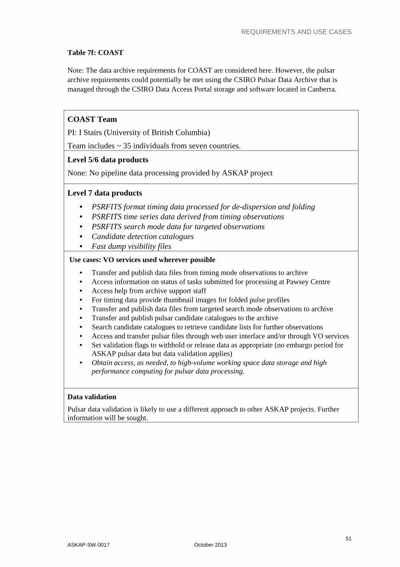
REQUIREMENTS AND USE CASES
51 ASKAP-SW-0017 October 2013
Table 7f: COAST Note: The data archive requirements for COAST are considered here. However, the pulsar archive requirements could potentially be met using the CSIRO Pulsar Data Archive that is managed through the CSIRO Data Access Portal storage and software located in Canberra.
COAST Team
PI: I Stairs (University of British Columbia)
Team includes ~ 35 individuals from seven countries.
Level 5/6 data products
None: No pipeline data processing provided by ASKAP project
Level 7 data products
• PSRFITS format timing data processed for de-dispersion and folding • PSRFITS time series data derived from timing observations • PSRFITS search mode data for targeted observations • Candidate detection catalogues • Fast dump visibility files
Use cases: VO services used wherever possible
• Transfer and publish data files from timing mode observations to archive • Access information on status of tasks submitted for processing at Pawsey Centre • Access help from archive support staff • For timing data provide thumbnail images for folded pulse profiles • Transfer and publish data files from targeted search mode observations to archive • Transfer and publish pulsar candidate catalogues to the archive • Search candidate catalogues to retrieve candidate lists for further observations • Access and transfer pulsar files through web user interface and/or through VO services • Set validation flags to withhold or release data as appropriate (no embargo period for
ASKAP pulsar data but data validation applies) • Obtain access, as needed, to high-volume working space data storage and high
performance computing for pulsar data processing.
Data validation
Pulsar data validation is likely to use a different approach to other ASKAP projects. Further information will be sought.

REQUIREMENTS AND USE CASES
52 ASKAP-SW-0017 October 2013
Table 7g: CRAFT
Note: CRAFT has challenging technical requirements (section 3.3.9). Data processing for CRAFT will be carried out by the science teams instead of as part of the ASKAP Science Data Processing pipelines. Although the data processing will be ‘offline’, CASDA may provide archive facilities for some CRAFT data products. The archive requirements for this project at the Pawsey Centre are not yet well established and further advice from the science team is sought.
Science Team
PI: R. Dodson (Korea Astronomy and Space Science Institute, Korea), J. P. Macquart (Curtin University)
Team includes ~ 40 individuals from four countries.
Level 5/6 data products
No pipeline data processing provided by ASKAP project
Level 7 data products (preliminary list only)
• Full baseband data recorded in data buffers during times of potential transient detections
• Event trigger information (time, flux, duration, frequency etc) • Images produced from buffered data for detected sources • Source-detection information for detected sources • Event handling information (community information, emails sent) • Source identifications and associations (possibly in real time) • Fast Transient Source Catalogue
.
Use cases
• Access summary information on observation blocks completed including information on system performance and RFI etc.
• Access information on status of tasks submitted for processing at Pawsey Centre • Access help from archive support staff • Load baseband data corresponding to the times of potential transient detections [or
possibly load these data after correlation and calibration?] • Load catalogues generated by science team • Access and retrieve information from catalogues • Load images generated by science team • Access and retrieve information from images • Set data release flag in CASDA after off-line data validation • Others [?]
Data validation
Further discussion is needed given to establish data validation procedures, given the stringent requirements to generate transient detections on very short timescales.
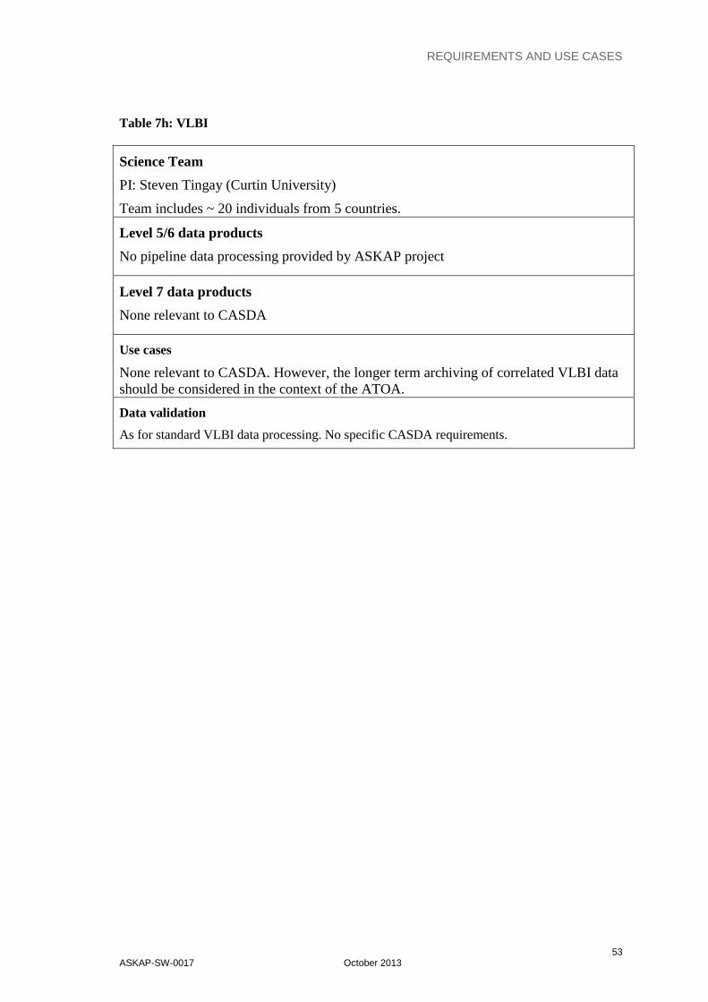
REQUIREMENTS AND USE CASES
53 ASKAP-SW-0017 October 2013
Table 7h: VLBI
Science Team
PI: Steven Tingay (Curtin University)
Team includes ~ 20 individuals from 5 countries.
Level 5/6 data products
No pipeline data processing provided by ASKAP project
Level 7 data products
None relevant to CASDA
Use cases
None relevant to CASDA. However, the longer term archiving of correlated VLBI data should be considered in the context of the ATOA.
Data validation
As for standard VLBI data processing. No specific CASDA requirements.
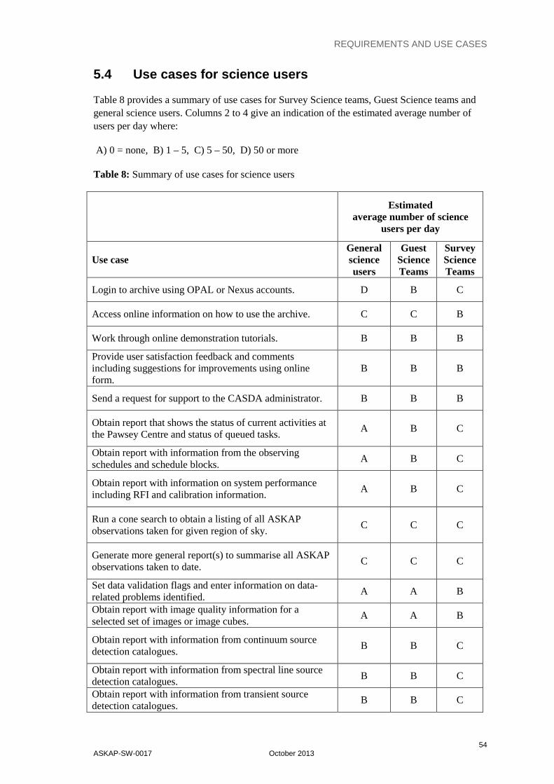
REQUIREMENTS AND USE CASES
54 ASKAP-SW-0017 October 2013
5.4 Use cases for science users
Table 8 provides a summary of use cases for Survey Science teams, Guest Science teams and general science users. Columns 2 to 4 give an indication of the estimated average number of users per day where:
A) 0 = none, B) 1 – 5, C) 5 – 50, D) 50 or more
Table 8: Summary of use cases for science users
Estimated average number of science
users per day
Use case General science users
Guest Science Teams
Survey Science Teams
Login to archive using OPAL or Nexus accounts. D B C
Access online information on how to use the archive. C C B
Work through online demonstration tutorials. B B B
Provide user satisfaction feedback and comments including suggestions for improvements using online form.
B B B
Send a request for support to the CASDA administrator. B B B
Obtain report that shows the status of current activities at the Pawsey Centre and status of queued tasks.
A B C
Obtain report with information from the observing schedules and schedule blocks.
A B C
Obtain report with information on system performance including RFI and calibration information.
A B C
Run a cone search to obtain a listing of all ASKAP observations taken for given region of sky.
C C C
Generate more general report(s) to summarise all ASKAP observations taken to date.
C C C
Set data validation flags and enter information on data-related problems identified.
A A B
Obtain report with image quality information for a selected set of images or image cubes.
A A B
Obtain report with information from continuum source detection catalogues.
B B C
Obtain report with information from spectral line source detection catalogues.
B B C
Obtain report with information from transient source detection catalogues.
B B C
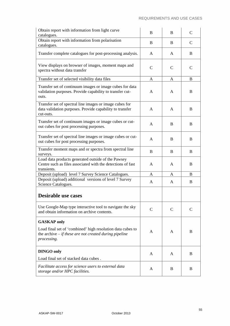
REQUIREMENTS AND USE CASES
55 ASKAP-SW-0017 October 2013
Obtain report with information from light curve catalogues.
B B C
Obtain report with information from polarisation catalogues.
B B C
Transfer complete catalogues for post-processing analysis. A A B
View displays on browser of images, moment maps and spectra without data transfer
C C C
Transfer set of selected visibility data files A A B
Transfer set of continuum images or image cubes for data validation purposes. Provide capability to transfer cut-outs.
A A B
Transfer set of spectral line images or image cubes for data validation purposes. Provide capability to transfer cut-outs.
A A B
Transfer set of continuum images or image cubes or cut-out cubes for post processing purposes.
A B B
Transfer set of spectral line images or image cubes or cut-out cubes for post processing purposes.
A B B
Transfer moment maps and or spectra from spectral line surveys.
B B B
Load data products generated outside of the Pawsey Centre such as files associated with the detections of fast transients.
A A B
Deposit (upload) level 7 Survey Science Catalogues. A A B Deposit (upload) additional versions of level 7 Survey Science Catalogues.
A A B
Desirable use cases
Use Google-Map type interactive tool to navigate the sky and obtain information on archive contents.
C C C
GASKAP only
Load final set of ‘combined’ high resolution data cubes to the archive – if these are not created during pipeline processing.
A A B
DINGO only
Load final set of stacked data cubes . A A B
Facilitate access for science users to external data storage and/or HPC facilities.
A B B

REQUIREMENTS AND USE CASES
56 ASKAP-SW-0017 October 2013
5.5 Use cases for Central Processor and archive administrators
Table 9 summarises use cases for accessing data from the Central Processor and for the administration of CASDA. Most of the CASDA administration and user support will be provided by CSIRO, with technical support for the Pawsey Centre infrastructure provided by iVEC.
Table 9: Summary of use cases for the Central Processor and archive administrators
Task Stakeholder
Ingest from the ASKAP Central Processor and Lustre file system metadata describing the science data products to be archived. This includes an enumeration of the data products, metadata describing the data products, and metadata describing the configuration of the telescope at the time the observations were carried out.
Central Processor
Ingest from the ASKAP Central Processor data product files for images and image cubes, visibilities and tables as are described by the metadata
Central Processor
Manage user access conditions: User groups include:
• Administrators and developers • Survey Science Team members • Guest Science Team members • General astronomy community
Administrators
Set proprietary period for Guest Science Projects (default is zero) where a proprietary period for a project is approved by the Time Assignment Committee.
Administrators
Manage archive queues. Assign priorities to tasks based on pre-determined conditions with goal of ensuring fair access.
Administrators
Adjust queues when needed to ensure fair access to archive services Administrators
Monitor system performance. Measures may include: Data transfer speeds between different system areas Amount of downtime due to CASDA faults Amount of downtime due to other (infrastructure) faults Response time to restore system following faults Percentage of data ‘lost’ in given year.
Administrators
Trigger alerts to archive administrators following any interruptions to normal performance.
Administrators

REQUIREMENTS AND USE CASES
57 ASKAP-SW-0017 October 2013
Provide statistical information on archive usage including: Number of users User demographics (CSIRO, Australia, overseas preferably by country) Volume of data transferred to other locations Volume of data archived to tape Volume of data recovered from tape
Administration
Transfer data from tape to disk.
Administration
Re-ingest a set of files after they have been modified. Update existing metadata in the archive database and associated indexes.
Administration
Regular backups of the science archive database and source catalogues
Administration

APPENDICES
58 ASKAP-SW-0017 October 2013
APPENDICES
Appendix A: Data volumes
The data volume for a set of correlated visibilities is given by:
N(beams) x N(pols) x N(channels) x N(baselines + autocorrelations) x Volume per visibility x Nsamples. The volume per complex visibility = 9 bytes. This includes 1 byte for weighting.
The number of samples = Total integration time/averaging time. The ASKAP averaging time for data sent from the correlator is 5s. For example, for a 12 hour observations Nsamples = 12x3600/5 = 8640.
The data volume for a ‘standard’ image cube is
Nx x Ny x Nchan x 4 bytes where:
Nx = number of pixels in one direction on the sky (usually right ascension or longitude)
Ny = number of pixels in the perpendicular direction on sky (usually declination or latitude)
Nchan = number of channels.
Note that for some observing modes (e.g. CRAFT), autocorrelations (total power) are output directly after the beam formers without using the ASKAP correlator.

APPENDICES
59 ASKAP-SW-0017 October 2013
Appendix B: CASDA data products
Table B1: CASDA Data Products
Visibility Data
Ref Visibility Data Sub-types
Stokes polarisation
products archived
Notes
P1 Calibrated continuum
visibility data Continuum only
I Q U V
Visibilities may be stored in either CASA
or FITS format.
Continuum frequency synthesis images
Image type Image sub-type (what the image measures)
Stokes polarisation
products Notes
P2 Restored
Intensity at fixed frequency Spectral index Spectral curvature
I
Three types of Taylor term images.
All image-related data products will be stored as FITS single-channel
image files.
P2 Residual
Intensity at fixed frequency Spectral index Spectral curvature
I
See above
P2 Model
Intensity at fixed frequency Spectral index Spectral curvature
I
See above
P2 Point spread function
Instrumental response to Point spread
I
P2 Sensitivity Sensitivity I
Continuum image cubes with polarisation
P2 Restored Intensity
I, Q, U, V Output as multi-
channel FITS format image cubes
P2 Residual Intensity I, Q, U, V
P2 Model Intensity I, Q, U, V
P2 Point spread function
Instrumental response to Point spread
I
P2 Sensitivity Sensitivity I
Spectral Line Image cubes and derived image product s
Type Image sub-type Polarisation
products Notes
P3 Image cubes Intensity I
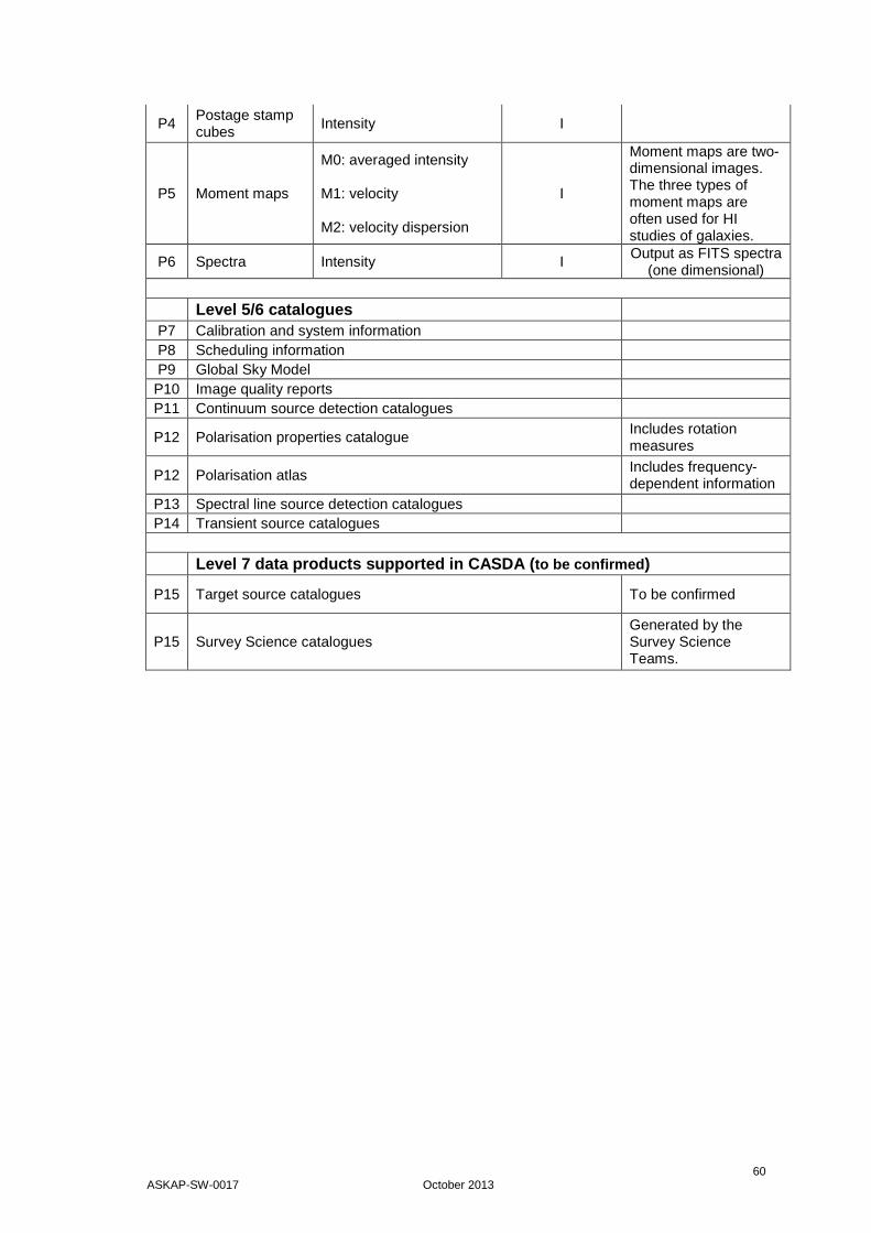
60 ASKAP-SW-0017 October 2013
P4 Postage stamp cubes
Intensity I
P5 Moment maps
M0: averaged intensity M1: velocity M2: velocity dispersion
I
Moment maps are two-dimensional images. The three types of moment maps are often used for HI studies of galaxies.
P6 Spectra Intensity I Output as FITS spectra (one dimensional)
Level 5/6 catalogues P7 Calibration and system information
P8 Scheduling information
P9 Global Sky Model
P10 Image quality reports
P11 Continuum source detection catalogues
P12 Polarisation properties catalogue
Includes rotation measures
P12 Polarisation atlas Includes frequency-dependent information
P13 Spectral line source detection catalogues
P14 Transient source catalogues
Level 7 data products supported in CASDA ( to be confirmed )
P15 Target source catalogues To be confirmed
P15 Survey Science catalogues Generated by the Survey Science Teams.

61 ASKAP-SW-0017 October 2013
Appendix C: Survey parameters
The tables in this appendix give parameters for the Survey Science Projects that will be processed at the Pawsey Centre. These are intended to indicate the data sizes for data processing and for archiving purposes. Values given correspond to different stages of the data flow, from the Telescope Operating System, through the data ingest, calibration and imaging pipelines to the archive. In most cases the parameters given are taken from [2].
Note that scheduling arrangements for ASKAP are not yet in place whilst the actual allocation of time and use of commensal observing are still to be determined. The tables correspond to indicative parameters for full ASKAP capabilities with 36 fully equipped antennas. In practice there will be an extended period between the start of Early Science and full array operation with data rates ramping up over time.
Table C1: Survey parameters for Emu and POSSUM
EMU POSSUM Project Information Project Code AS014 AS007 Rating 1 2 Survey type Continuum Continuum
Array Parameters Number of antennas 36 36 Maximum baseline (km) 6 6
Number of baselines (includes autocorrelations) 666 666 Number of beams 36 36
Frequency channels from the correlator 16,200 16,200 Number of polarisations 4 4 Frequency channels after averaging 300 300 Data sizes and rates Bytes per complex sample (includes 1 for weight) 9 9
Data volume per visibility data set (GB) 13.98 13.98 Number of polarisations 4 4 Integration time (s) 5 5
Data rate (Gbits/s): Correlator to Real Time Computer prior to channel averaging 22.37 22.37
Averaged visibility frame (GB) 0.26 0.26 Averaged data rate (GB/s) 0.052 0.052 Averaged data rate (TB/h) 0.19 0.19
Observing time (h) 12 8
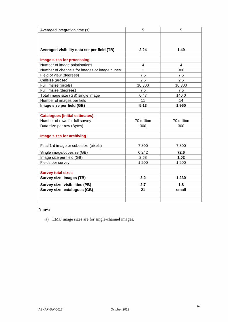
62 ASKAP-SW-0017 October 2013
Averaged integration time (s) 5 5
Averaged visibility data set per field (TB) 2.24 1. 49 Image sizes for processing Number of image polarisations 4 4 Number of channels for images or image cubes 1 300 Field of view (degrees) 7.5 7.5 Cellsize (arcsec) 2.5 2.5 Full Imsize (pixels) 10,800 10,800 Full Imsize (degrees) 7.5 7.5 Total image size (GB) single image 0.47 140.0 Number of images per field 11 14 Image size per field (GB) 5.13 1,960 Catalogues [initial estimates]
Number of rows for full survey 70 million 70 million Data size per row (Bytes) 300 300 Image sizes for archiving
Final 1-d image or cube size (pixels) 7,800 7,800
Single image/cubesize (GB) 0.242 72.6 Image size per field (GB) 2.68 1.02 Fields per survey 1,200 1,200
Survey total sizes Survey size: images (TB) 3.2 1,230
Survey size: visibilities (PB) 2.7 1.8 Survey size: catalogues (GB) 21 small
Notes:
a) EMU image sizes are for single-channel images.

63 ASKAP-SW-0017 October 2013
Table C2: Survey parameters for WALLABY
WALLABY 2-km array
Postage stamps set (a)
Postage stamps set
(b) Project Information Project Code AS016 Rating 1 Survey type SL
Array Parameters Number of antennas 36 Maximum baseline (km) 2 6 6
Number of baselines (includes autocorrelations) 666 Number of beams 36
Frequency channels from the correlator 16,200 Number of polarisations 4
Frequency channels after averaging 16,200
Data sizes and rates
Bytes per complex sample (includes 1 for weight) 9
Raw visibility frame - all pols (GB) 13.98 Number of polarisations 4 Integration time (s) 5 Data rate (Gbits/s) 22.37
Visibility frame after any channel averaging (GB) 13.98 Averaged data rate (GB/s) 2.8 Averaged data rate (TB/h) 10.08
Observation time per field (h) 8 Averaged visibility data set per field (TB) 80.54
Image sizes for processing
Number of image polarisations 1 1 1
Number of channels for images or image cubes 16,200 512 16,200 1-d field of view (degrees) 7.5 0.178 0.089 Cellsize (arcsec) 7.5 2.5 2.5 Full Imsize (pixels) 3600 256 128 Full Imsize (degrees) 7.5 0.178 0.089
Total image size (GB) single image 839 0.134 1.06 Number of images per field 3 1050 3000 Image size per field (TB) 2.5 0.14 3.18
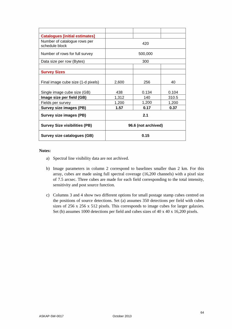
64 ASKAP-SW-0017 October 2013
Catalogues [initial estimates] Number of catalogue rows per schedule block
420
Number of rows for full survey 500,000
Data size per row (Bytes) 300 Survey Sizes
Final image cube size (1-d pixels) 2,600 256 40
Single image cube size (GB) 438 0.134 0.104 Image size per field (GB) 1,312 140 310.5 Fields per survey 1,200 1,200 1,200 Survey size images (PB) 1.57 0.17 0.37
Survey size images (PB) 2.1
Survey Size visibilities (PB) 96.6 (not archived)
Survey size catalogues (GB) 0.15
Notes:
a) Spectral line visibility data are not archived.
b) Image parameters in column 2 correspond to baselines smaller than 2 km. For this array, cubes are made using full spectral coverage (16,200 channels) with a pixel size of 7.5 arcsec. Three cubes are made for each field corresponding to the total intensity, sensitivity and post source function.
c) Columns 3 and 4 show two different options for small postage stamp cubes centred on the positions of source detections. Set (a) assumes 350 detections per field with cubes sizes of 256 x 256 x 512 pixels. This corresponds to image cubes for larger galaxies. Set (b) assumes 1000 detections per field and cubes sizes of 40 x 40 x 16,200 pixels.

65 ASKAP-SW-0017 October 2013
Table C3: Survey parameters for DINGO and FLASH
DINGO FLASH Project Information
Project Code AS012 AS002 Rating 1 1 Survey type SL SL
Array Parameters
Number of antennas 36 36 Maximum baseline (km) 2 6
Number of baselines (includes autocorrelations) 666 666 Number of beams 36 36
Frequency channels from the correlator 16,200 16,200 Number of polarisations 4 4
Frequency channels after averaging 16,200 16,200
Data sizes and rates
Bytes per complex sample (includes 1 for weight) 9 9
Raw visibility frame - all pols (GB) 13.98 13.98 Number of polarisations 4 4 Integration time (s) 5 5 Data rate (Gbits/s) 22.37 22.37
Visibility frame after any channel averaging (GB) 13.98 13.98 Averaged data rate (GB/s) 2.8 2.8 Averaged data rate (TB/h) 10.08 10.08
Observation time per field (h) 8 4
Averaged visibility data set per field (TB) 80.54 40.27
Image sizes for processing
Number of image polarisations 1 1
Number of channels for images or image cubes 16,200 16,200 1-d field of view (degrees) 7.5 0.089 Cellsize (arcsec) 7.5 2.5 Full Imsize (pixels) 3600 128 Full Imsize (degrees) 7.5 0.089
Total image size (GB) single image 839 1.062 Number of images per field 3 450 Image size per field (TB) 2.5 0.48
Catalogues [initial estimates]
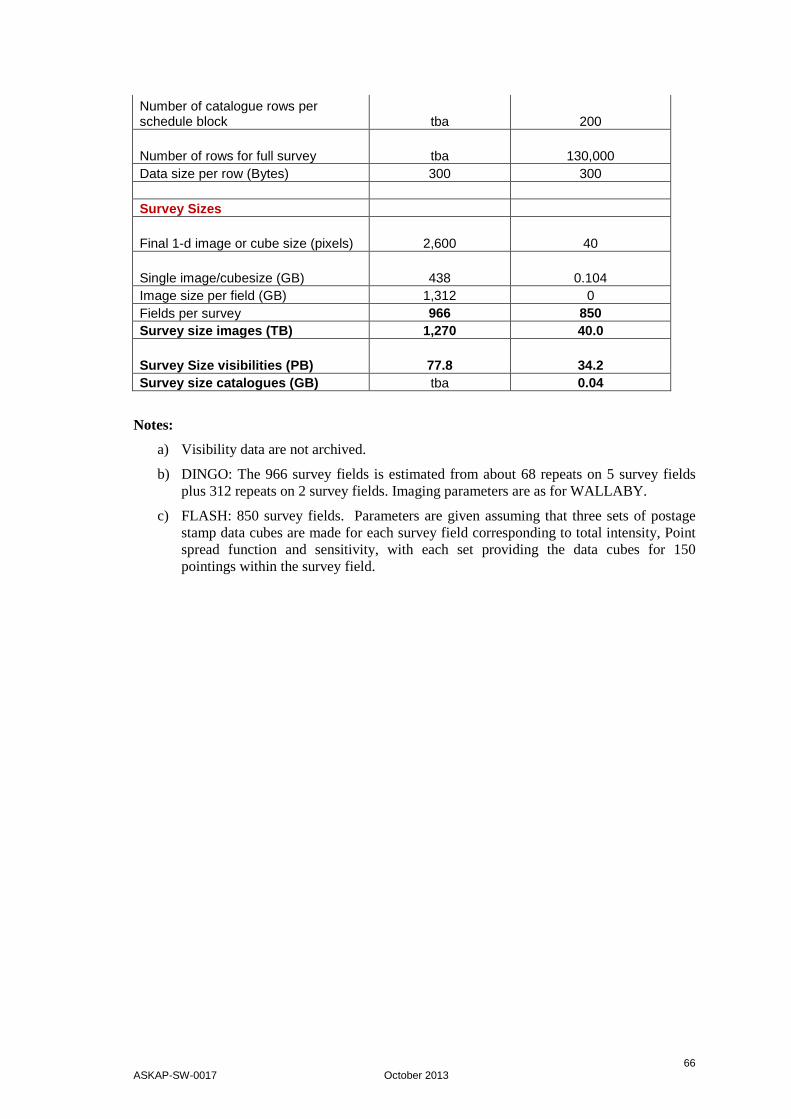
66 ASKAP-SW-0017 October 2013
Number of catalogue rows per schedule block tba 200
Number of rows for full survey tba 130,000 Data size per row (Bytes) 300 300
Survey Sizes
Final 1-d image or cube size (pixels) 2,600 40
Single image/cubesize (GB) 438 0.104 Image size per field (GB) 1,312 0 Fields per survey 966 850 Survey size images (TB) 1,270 40.0
Survey Size visibilities (PB) 77.8 34.2 Survey size catalogues (GB) tba 0.04
Notes:
a) Visibility data are not archived.
b) DINGO: The 966 survey fields is estimated from about 68 repeats on 5 survey fields plus 312 repeats on 2 survey fields. Imaging parameters are as for WALLABY.
c) FLASH: 850 survey fields. Parameters are given assuming that three sets of postage stamp data cubes are made for each survey field corresponding to total intensity, Point spread function and sensitivity, with each set providing the data cubes for 150 pointings within the survey field.

67 ASKAP-SW-0017 October 2013
Table C4: Survey parameters for GASKAP
2-km array Postage stamps Project Information
Project Code AS005
Rating 2 Survey type SL Array Parameters Number of antennas 36 Maximum baseline (km) 2
Number of baselines (includes autocorrelations)
666
Number of beams 36 Frequency channels from the correlator
16,200
Number of polarisations 4
Frequency channels after averaging 16,200
Data sizes and rates Bytes per complex sample (includes 1 for weight)
9
Raw visibility frame - all pols (GB) 13.98 Number of polarisations 4 Integration time (s) 5 Data rate (Gbits/s) 22.37 Visibility frame after any channel averaging (GB)
13.98
Averaged data rate (GB/s) 2.8 Averaged data rate (TB/h) 10.08
Observation time per field (h) 12.5
Averaged visibility data set per field (TB)
125.8
Image sizes for processing
Number of image polarisations 1 1
Number of channels for image cubes 16,200 16,200
1-d field of view (degrees) 7.5 0.089 Cellsize (arcsec) 7.5 2.5 Full Imsize (pixels) 3,600 128 Full Imsize (degrees) 7.5 0.089
Total image size (GB) single image 839 1.06
Number of images per field 3 50 Image size per field (GB) 2517 53 Catalogues [initial estimates]

68 ASKAP-SW-0017 October 2013
Number of catalogue rows per schedule block
50
Number of rows for full survey 30000
Data size per row (Bytes) 300 Survey Sizes
Final 1-d image or cube size (pixels) 2600 128
Single image/cubesize (GB) 438 1.06
Image size per field (GB) 1312 53.0 Schedule blocks per survey 644 Fields per survey 481
Survey size image cubes (TB) 846 34
Survey size – all image cubes TB) 880
Survey Size visibilities (PB) 125.8
Survey size catalogues (MB) 9 Notes:
a) Parameters for GASKAP are adapted from [9]. Total observing time of 8050 hours is assumed to be taken over 644 blocks of 12.5 hours. To increase the sensitivity, some fields are observed more than once.
b) Observations will be taken using three zoom bands to cover the frequency ranges for HI, OH 1612 MHz and OH 1665/1667 MHz.
c) To estimate the data volumes, parameters are given for spectral line cubes with 16200 channels. In these will be generated as three smaller cubes with 50%, 25% and 25% of the channels correspond to the three zoom bands respectively.
d) A total of 30,000 point-like source detections is assumed (approximately 15,000 for HI
and 15,000 for OH). This corresponds to an average of about 50 detections per 12.5 schedule block.
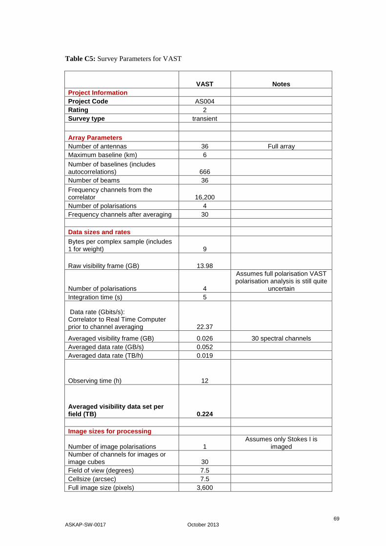
69 ASKAP-SW-0017 October 2013
Table C5: Survey Parameters for VAST VAST Notes Project Information
Project Code AS004 Rating 2
Survey type transient
Array Parameters Number of antennas 36 Full array
Maximum baseline (km) 6
Number of baselines (includes autocorrelations) 666 Number of beams 36
Frequency channels from the correlator 16,200 Number of polarisations 4 Frequency channels after averaging 30
Data sizes and rates Bytes per complex sample (includes
1 for weight) 9
Raw visibility frame (GB) 13.98
Number of polarisations 4
Assumes full polarisation VAST polarisation analysis is still quite
uncertain Integration time (s) 5
Data rate (Gbits/s): Correlator to Real Time Computer prior to channel averaging 22.37
Averaged visibility frame (GB) 0.026 30 spectral channels Averaged data rate (GB/s) 0.052 Averaged data rate (TB/h) 0.019
Observing time (h) 12
Averaged visibility data set per field (TB) 0.224
Image sizes for processing
Number of image polarisations 1 Assumes only Stokes I is
imaged Number of channels for images or image cubes 30 Field of view (degrees) 7.5 Cellsize (arcsec) 7.5 Full image size (pixels) 3,600

70 ASKAP-SW-0017 October 2013
Full imsize (degrees) 7.5 Total image size (GB) single image 1.56 Number of images per field 8,640 For 12 hours observing Total image volume for 12 hours (TB) 13.4
Catalogues [initial estimates] Number of catalogue rows for full
survey 5.2 billion No compression Data size per row (Bytes) 300
Image sizes for archiving
Final 1-d image or cube size (pixels) 2,600
Single image/cubesize (GB) 0.81 Image size per field (GB) 7,000 8640 image cubes in 12 hours.
Fields per survey 1,200 Piggy-back mode
Survey total sizes
Survey size: images (PB) 8.4 Total image volume generated after 1200 blocks of 12 hours
Survey size: visibilities (PB) 0.27 Survey size: catalogues (GB) see note (c)
Notes
a) VAST observations may be taken using a wide range of parameters depending on the system set up for other scheduled projects. The parameters given here correspond to 12 hours of observations with 30 spectral channels and full polarisation visibility data retained with images formed for one polarisation only.
b) The full-sized VAST image cubes are unlikely to be retained. However, postage stamp image cubes for potential transient detections may be archived.
c) The number of catalogue rows for VAST is potentially very large. The number of rows given here (five billion) is based on an estimate of 500 detections every five seconds with every detection retained as a separate row. With no data compression the approximate size of a catalogue would be about 1.5 TB. However, by splitting the information, into separate catalogues for source detections and light curves, it should be possible to greatly compress the data volume for the transient catalogues to manageable levels below ~50 GB.

REFERENCES
71 ASKAP-SW-0017 October 2013
REFERENCES
[1] Bock, D., Chapman, J., Lensson, E., Edwards, P., (2012), ATNF Operations in the ASKAP Era, version B
[2] Cornwell, T, Humphreys, B., Lenc, E., Voronkov, M., Whiting, M., (2011) ASKAP Science Processing, ASKAP-SW-0020
[3] Feian, et al., (2009), ASKAP User Policy, http://www.atnf.csiro.au/projects/askap/UserPolicy_final.pdf
[4] Humphreys, B., (2011) ASKAP Central Processor Pawsey Centre Requirements Document, ASKAP-SW-0021
[5] Humphreys, B., Guzman, J.C., Marquarding, M., Cornwell, T., Voronkov, M., Brodrick, D., ASKAP Computing Architecture, ASKAP-SW-0003
[6] Norris, R., Johnston, S., (2009), ASKAP Science Data Archive: Draft Requirements Document, ASKAP-SC-0001, version 1.0
[7] Whiting, M., (2012), Duchamp: a 3D source finder for spectral-line data, MNRAS, 421, 3242
[8] Whiting, M., Humphreys, B., (2012), Source-finding for the Australian Square Kilometre Array Pathfinder, PASA, 29, 371 – 381
[9] Dickey, J. M., McClure-Griffiths, N. et al., (2013) The Galactic ASKAP Survey, PASA 30,3
[10] ASKAP Requirements, (2013), version 0.2, ASKAP-SEIC-0007
[11] Lorimer, D., et al., (2007), A Bright Millisecond Radio Burst of Extragalactic Origin, Science, 318, 777
[12] Thornton et al., (2013), A Population of Fast Radio Bursts at Cosmological Distances, Science, 341, 53