CT Scanner and Applications in Soil Science:

Fundamentals, X-ray Sensors and Detectors,

Architectures and Algorithms for Image

Reconstruction and Scientific Visualization

Paulo E. Cruvinel, Ph.D. paulo.cruvinel@embrapa.br

What is X-Ray Computed Tomography (CT)?

• Considering a short definition CT, which is also referred to as CAT, for Computed Axial Tomography, utilizes X-ray technology and sophisticated instrumentation, sensors & computers to create images of cross-sectional “slices” through a body under analysis. • CT exams and CAT scanning provide a quick overview of morphologies and its quantification (also those related to pathologies) and enable rapid analysis and plans for prognostics and support for decision maker. • Tomography is a term that refers to the ability to view an anatomic section or slice through the body. • Anatomic cross sections are most commonly refers to transverse axial tomography

What is displayed in CT images?

HU1000CT# T

water

water

Water: 0HU

Air: -1000HU

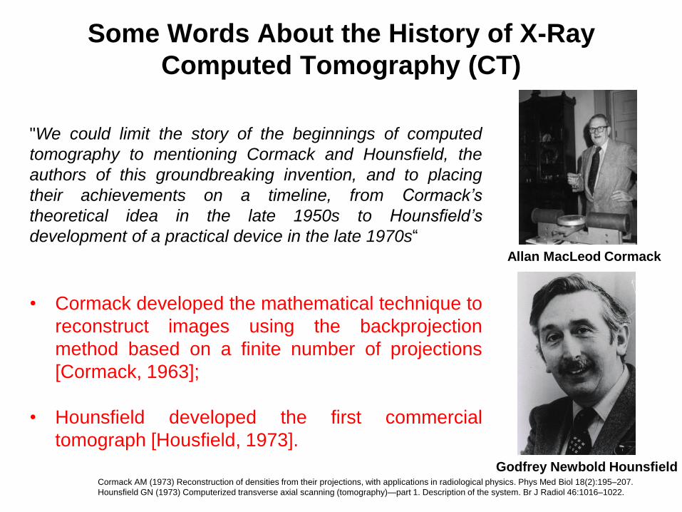
Some Words About the History of X-Ray

Computed Tomography (CT)

"We could limit the story of the beginnings of computed

tomography to mentioning Cormack and Hounsfield, the

authors of this groundbreaking invention, and to placing

their achievements on a timeline, from Cormack’s

theoretical idea in the late 1950s to Hounsfield’s

development of a practical device in the late 1970s“

• Cormack developed the mathematical technique to

reconstruct images using the backprojection

method based on a finite number of projections

[Cormack, 1963];

• Hounsfield developed the first commercial

tomograph [Housfield, 1973].

Cormack AM (1973) Reconstruction of densities from their projections, with applications in radiological physics. Phys Med Biol 18(2):195–207.

Hounsfield GN (1973) Computerized transverse axial scanning (tomography)—part 1. Description of the system. Br J Radiol 46:1016–1022.

Allan MacLeod Cormack

Godfrey Newbold Hounsfield

Radon, Johann (1917), "Über die Bestimmung von Funktionen durch ihre Integralwerte längs gewisser Mannigfaltigkeiten", Berichte über die Verhandlungen der Königlich-

Sächsischen Akademie der Wissenschaften zu Leipzig, Mathematisch-Physische Klasse [Reports on the proceedings of the Royal Saxonian Academy of Sciences at

Leipzig, mathematical and physical section], Leipzig: Teubner (69): 262–277; Translation: Radon, J.; Parks, P.C. (translator) (1986), "On the determination of functions from

their integral values along certain manifolds", IEEE Transactions on Medical Imaging, 5 (4): 170–176.

Johann Karl August Radon

In mathematics, the Radon transform is the integral

transform which takes a function f defined on the plane

to a function Rf defined on the space of lines in the

plane, whose value at a particular line is equal to

the line integral of the function over that line (introduced

in 1917 and also provided a formula for the inverse

transform).

• Radon (1887- 1956) presents the mathematical principles of a body

reconstruction from their projections considering a space with order

equal to n [Radon, 1917];

• CT uses electromagnetic wave, i.e., X-radiation.

Michael Faraday (1791–1867)

observed the phenomenon of

electromagnetism and in 1831

formulated the laws of

electromagnetic induction.

Twenty-nine years later, in 1860, James

Clark Maxwell (1831-1879), formulates the

Maxwell’s equations, comprehensively

expressed the ideas of electricity and

magnetism, which led to the development

of the later technologies of radio and

television and of course, radiology.

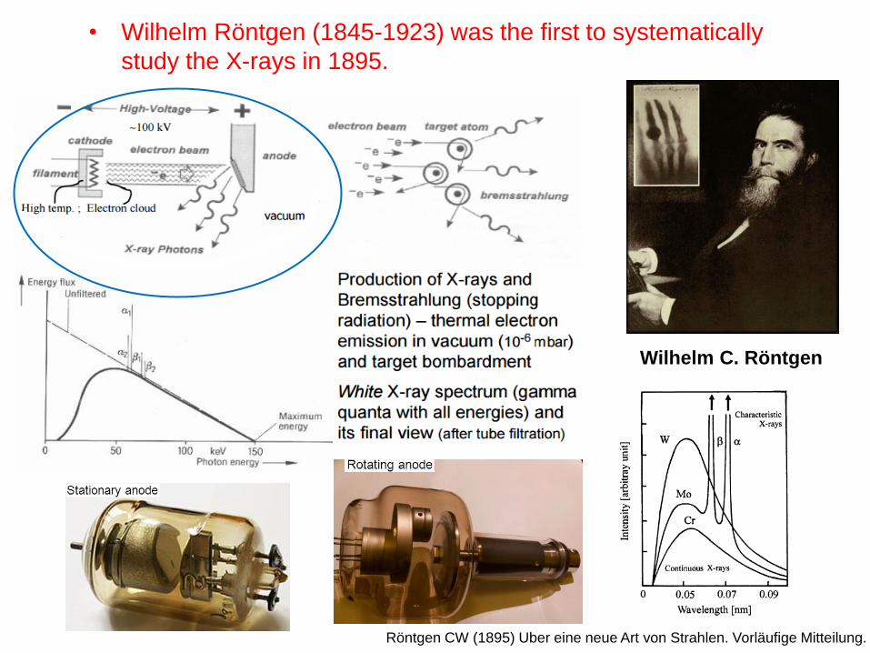
Wilhelm C. Röntgen

• Wilhelm Röntgen (1845-1923) was the first to systematically

study the X-rays in 1895.

Röntgen CW (1895) Uber eine neue Art von Strahlen. Vorläufige Mitteilung.

The Nobel Prize in Physiology or Medicine 1979

Region of Interest (electromagnetic spectrum) for CT

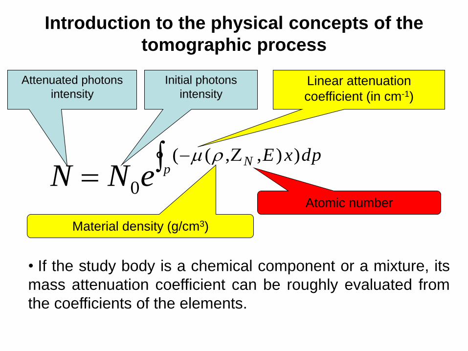
Introduction to the physical concepts of the

tomographic process

• The bases of the X-ray transmission tomography are

related to a narrow beam of monoenergetic photons

with energy E and a flux of photons N0 passing through

a homogeneous body of thickness x (in cm):

0N

x

N

X-Ray source Detector

E

),,( EN

p

N dpxE

eNN)),,((

0

Material density (g/cm3)

Atomic number

Linear attenuation

coefficient (in cm-1)

Initial photons

intensity

Attenuated photons

intensity

• If the study body is a chemical component or a mixture, its

mass attenuation coefficient can be roughly evaluated from

the coefficients of the elements.

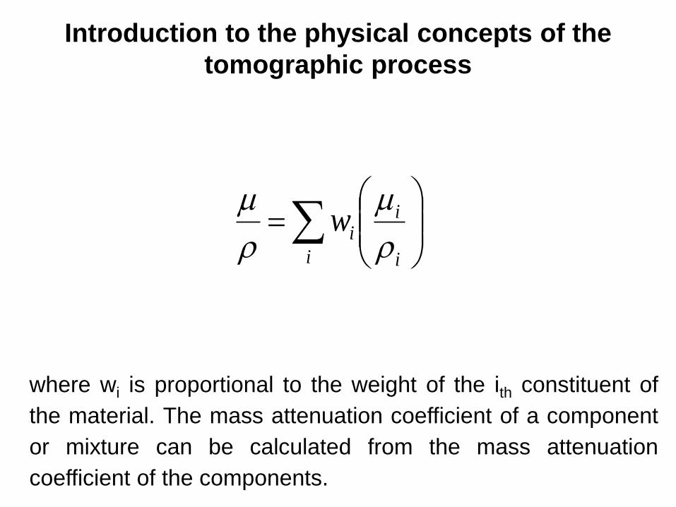
Introduction to the physical concepts of the

tomographic process

i

i

i

iw

Introduction to the physical concepts of the

tomographic process

where wi is proportional to the weight of the ith constituent of

the material. The mass attenuation coefficient of a component

or mixture can be calculated from the mass attenuation

coefficient of the components.

0

1

2

3

4

5

6

7

30 58 114 222 433

(c

m-1

)

Energy (keV)

Introduction to the physical concepts of the

tomographic process

(Ca)

This fact leads to a definition of the contrast in X-ray computed tomography,

which is a function of the linear attenuation coefficient values

and the mapping process.

The differences in linear attenuation coefficients for different

materials are energy dependent.

0

1

2

3

4

5

6

7

30 58 114 222 433

(c

m-1

)

Energy (keV)

Al Ca K

The quality of a tomographic image is correlated to the work energy, as well as the physical characteristics of the samples or bodies under analysis (function of the chemical constituents).

Introduction to the physical concepts of the

tomographic process

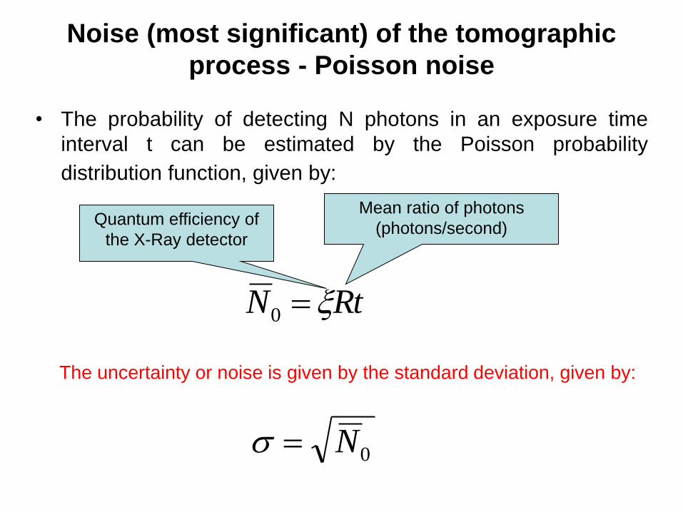
Noise (most significant) of the tomographic

process - Poisson noise

• The probability of detecting N photons in an exposure time

interval t can be estimated by the Poisson probability

distribution function, given by:

RtN 0

Mean ratio of photons

(photons/second) Quantum efficiency of

the X-Ray detector

0N

The uncertainty or noise is given by the standard deviation, given by:

An event can occur 0, 1, 2, … times in an interval. The average number

of events in an interval is designated . It is the event rate, also called the

rate parameter. The probability of observing k events in an interval is

given by the equation:

where:

is the average number of events per interval

e is the number 2.71828... (Euler's number) the

base of the natural logarithms

k takes values 0, 1, 2, …

k! = k × (k − 1) × (k − 2) × … × 2 × 1 is

the factorial of k.

!),(

ktkP e

k

Probability mass function (PMF)

for a Poisson distribution

Sample scanning process

• Two-dimensional reconstruction

algorithms use projections to

reconstruct the tomographic

sections;

• Projections are collected in the

interval

i.e., getting the Radon transform of

the object;

• Through the inverse transform of

Radon one can obtain the

reconstructed image of the

object, based on the attenuation

coefficients

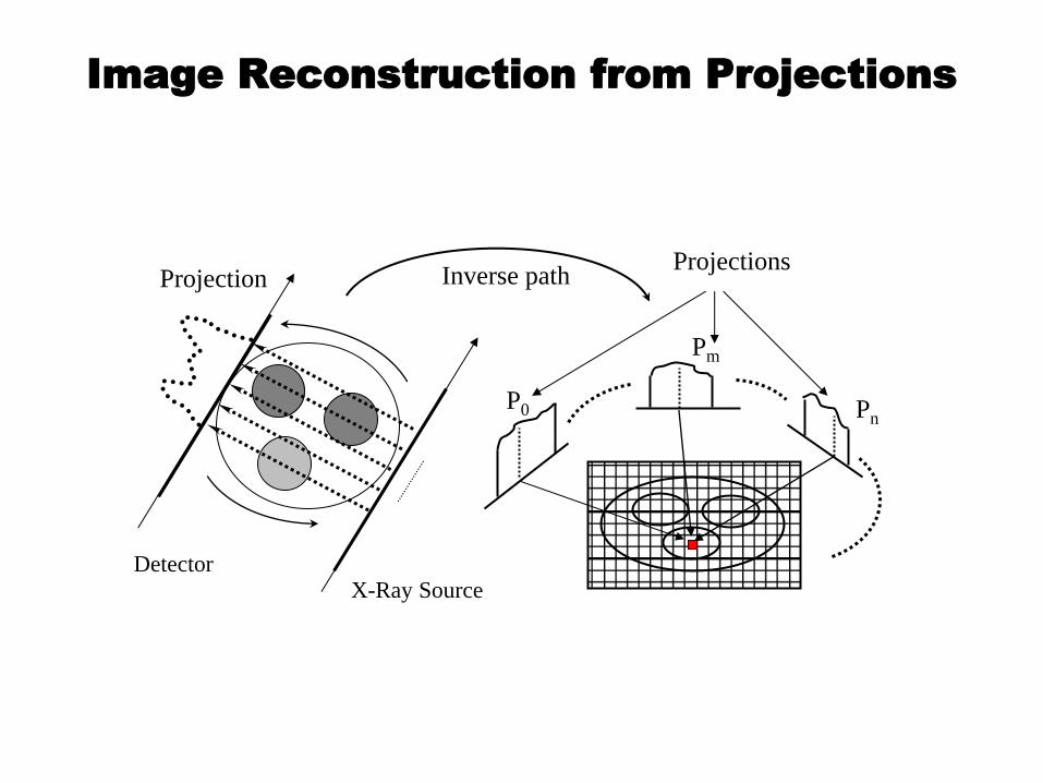
Image Reconstruction from Projections

Projection

X-Ray Source Detector

Inverse path Projections

P0

Pm

Pn

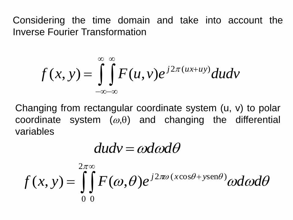
dudvevuFyxf uyuxj )(2),(),(

dddudv

Considering the time domain and take into account the

Inverse Fourier Transformation

2

0 0

)sencos(2),(),( ddeFyxf yxj

Changing from rectangular coordinate system (u, v) to polar

coordinate system (,) and changing the differential

variables

)]([)](ˆ[)( nhFFTnPFFTIFFTnQ

where is the sampling interval

)]([)]([)( nhFFTnPFFTIFFTnQ

K

i

ii senyxQK

yxf1

)cos(),(ˆ

Using discrete forms to represent de projections and

rewritten the equations in the frequency domain, is possible

to find:

Reconstruction from projections

CT without covers

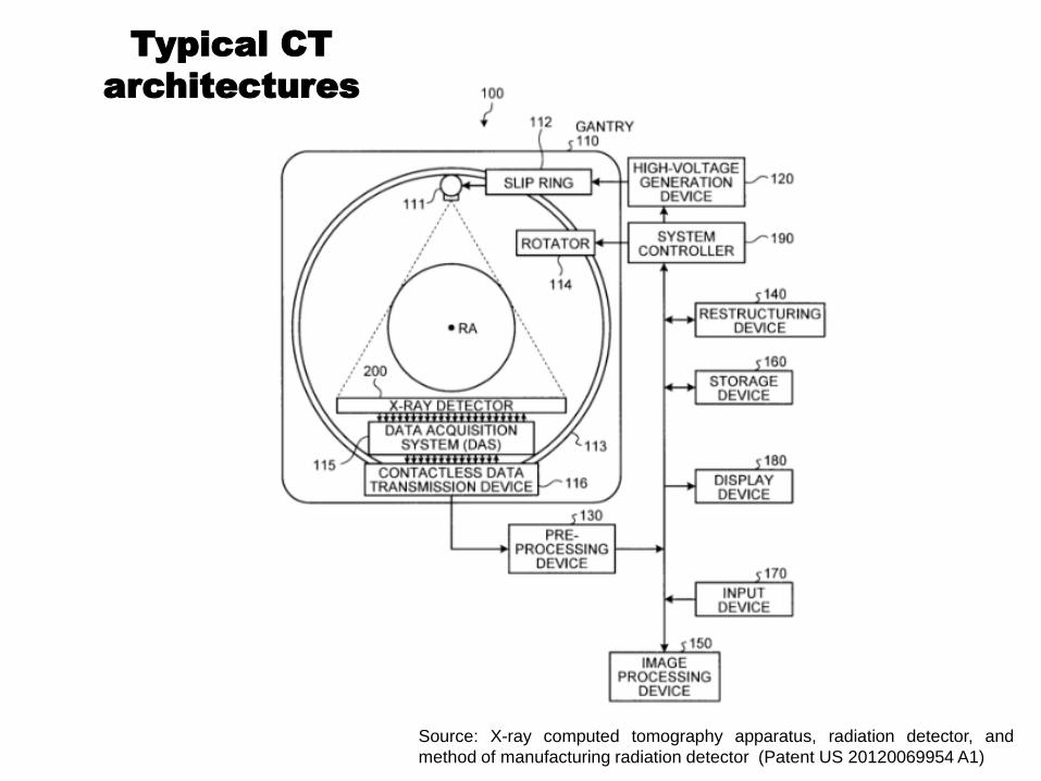
Source: X-ray computed tomography apparatus, radiation detector, and

method of manufacturing radiation detector (Patent US 20120069954 A1)

Typical CT

architectures

Typical Schematic Representation for Scanning

Geometry of a CT System

What are inside the gantry?

CT System & Generations

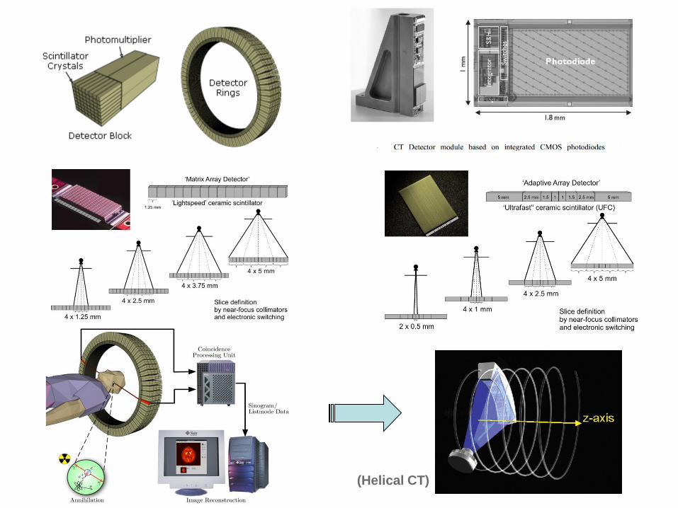
(Helical CT)

Source: Imaging Systems for Medical Diagnosis: Fundamentals and Technical Solutions - X-Ray Diagnostics- Computed Tomography - Nuclear Medical Diagnostics

- Magnetic Resonance Imaging - Ultrasound Technology, by Erich Krestel (Editor), pp. 627. ISBN 3-8009-1564-2. Wiley-VCH , October 1990.

SNR is dependent on dose, as in

X-ray. Notice how images become

grainier and our ability to see small

objects decreases as dose

decreases.

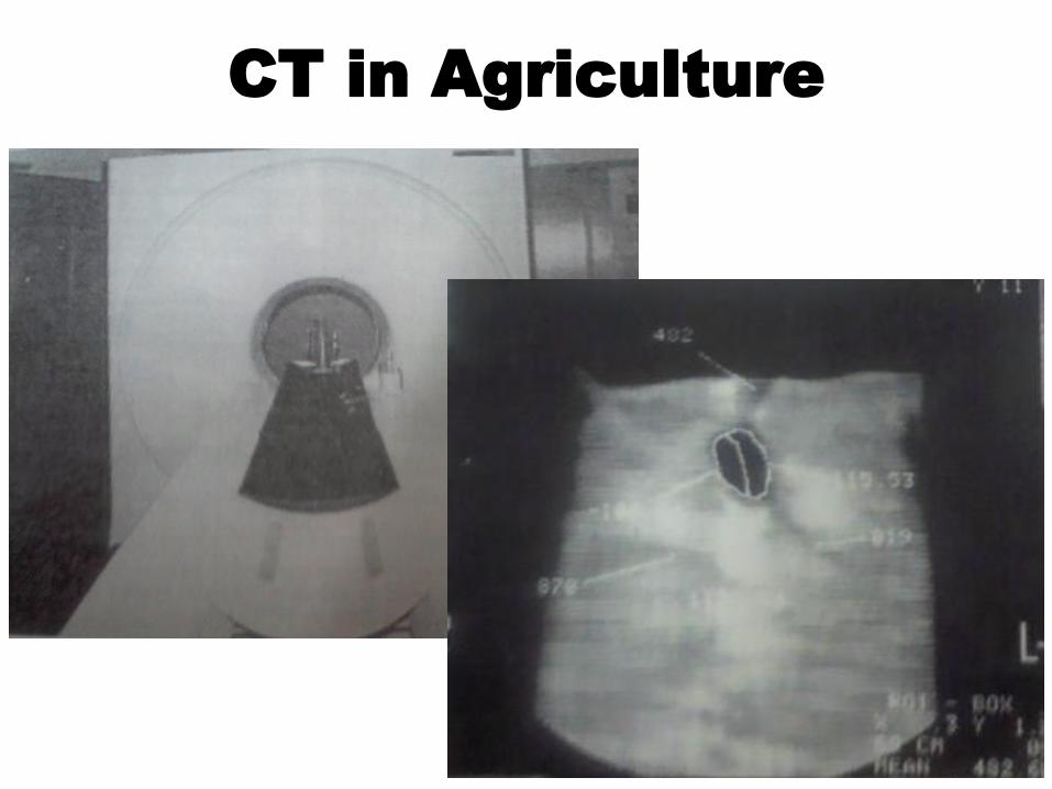
CT in Agriculture

• In 1982 and 1983 studies were conducted respectively by Petrovic &

Hainsworth, and Aylmore. They demonstrated the possibility of using a

computerized X-ray tomograph to measure the bulk density of soils;

• In 1986, Crestana and collaborators presented results related to the

applications of CT in agriculture for:

1. Detection of soil heterogeneities;

2. Compaction of soils resulting from the use of agricultural machinery;

3. Dynamic three-dimensional simulation of drip irrigation in a soil column;

4. Studies on seed germination in situ.

Their results were compared with usual techniques in the agricultural area

the use of CT showed greater precision.

Crestana, S.; Mascarenhas, S.; Pozzi-mucelli, R.S. Static and dynamic three-dimensional studies of water in soil using computed tomographic scanning. Soil Science, v.140,

p.326-332,1985.; Aylmore, L. A. G. Use of computer-assisted tomography in studying water movement around plant roots. Advances in Agronomy, San Diego, v. 49, p. 1-53,

1993.; Petrovic, A.M.; Siebert, J.E.; Rieke, P.E. Soil bulk density analysis in three dimensions by computed tomographic scanning. Soil Science Society of America Journal,

v.46, p.445-450, 1982.

CT in Agriculture

CT in Agriculture

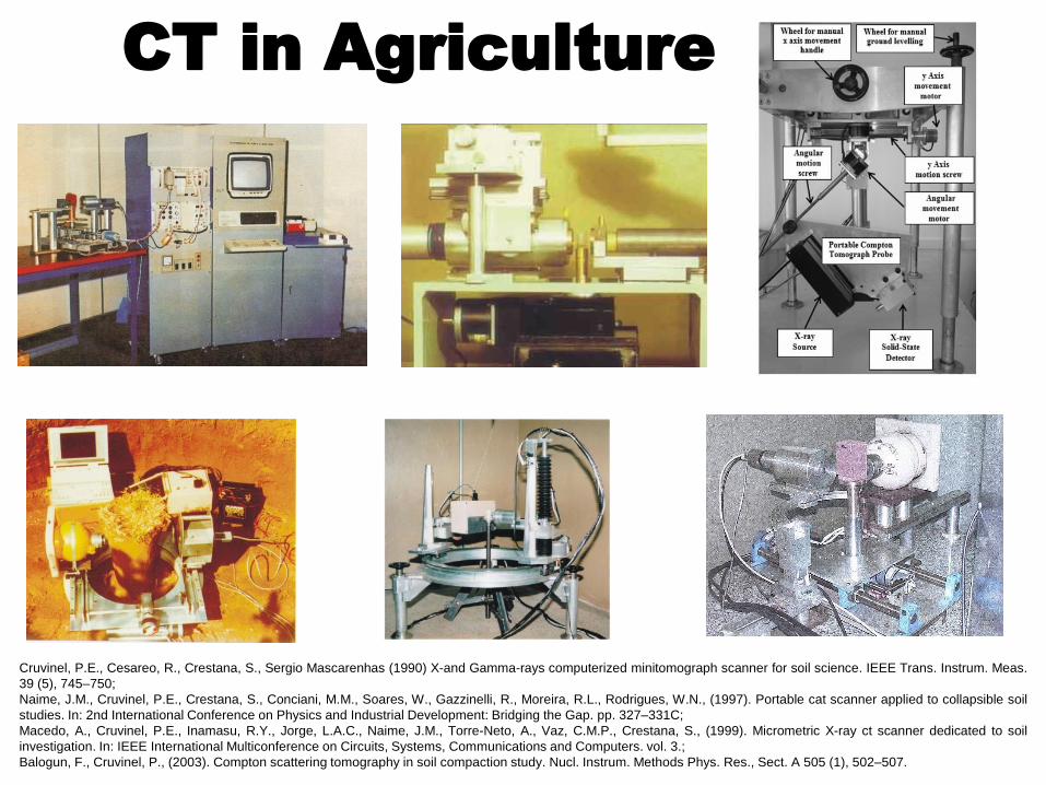
CT in Agriculture

Cruvinel, P.E., Cesareo, R., Crestana, S., Sergio Mascarenhas (1990) X-and Gamma-rays computerized minitomograph scanner for soil science. IEEE Trans. Instrum. Meas.

39 (5), 745–750;

Naime, J.M., Cruvinel, P.E., Crestana, S., Conciani, M.M., Soares, W., Gazzinelli, R., Moreira, R.L., Rodrigues, W.N., (1997). Portable cat scanner applied to collapsible soil

studies. In: 2nd International Conference on Physics and Industrial Development: Bridging the Gap. pp. 327–331C;

Macedo, A., Cruvinel, P.E., Inamasu, R.Y., Jorge, L.A.C., Naime, J.M., Torre-Neto, A., Vaz, C.M.P., Crestana, S., (1999). Micrometric X-ray ct scanner dedicated to soil

investigation. In: IEEE International Multiconference on Circuits, Systems, Communications and Computers. vol. 3.;

Balogun, F., Cruvinel, P., (2003). Compton scattering tomography in soil compaction study. Nucl. Instrum. Methods Phys. Res., Sect. A 505 (1), 502–507.

Model and Algorithm Conception

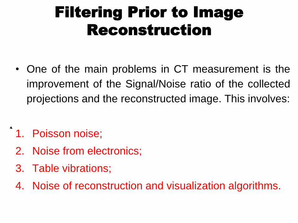
Filtering Prior to Image

Reconstruction

• One of the main problems in CT measurement is the

improvement of the Signal/Noise ratio of the collected

projections and the reconstructed image. This involves:

1. Poisson noise;

2. Noise from electronics;

3. Table vibrations;

4. Noise of reconstruction and visualization algorithms.

• Regarding Poisson noise, the possible solutions are:

1. Increase the exposure time to radiation, to improve the

signal-to-noise ratio;

2. Applying filtering to reduce Poisson noise, working on

the projections, or a posteriori in the reconstructed

image.

Anscombe

Transform

Prior filtering

by Wiener or

Kalman

Inverse

Anscombe

Transform

Projections Filtered

Projections

Filtering Prior to Image

Reconstruction

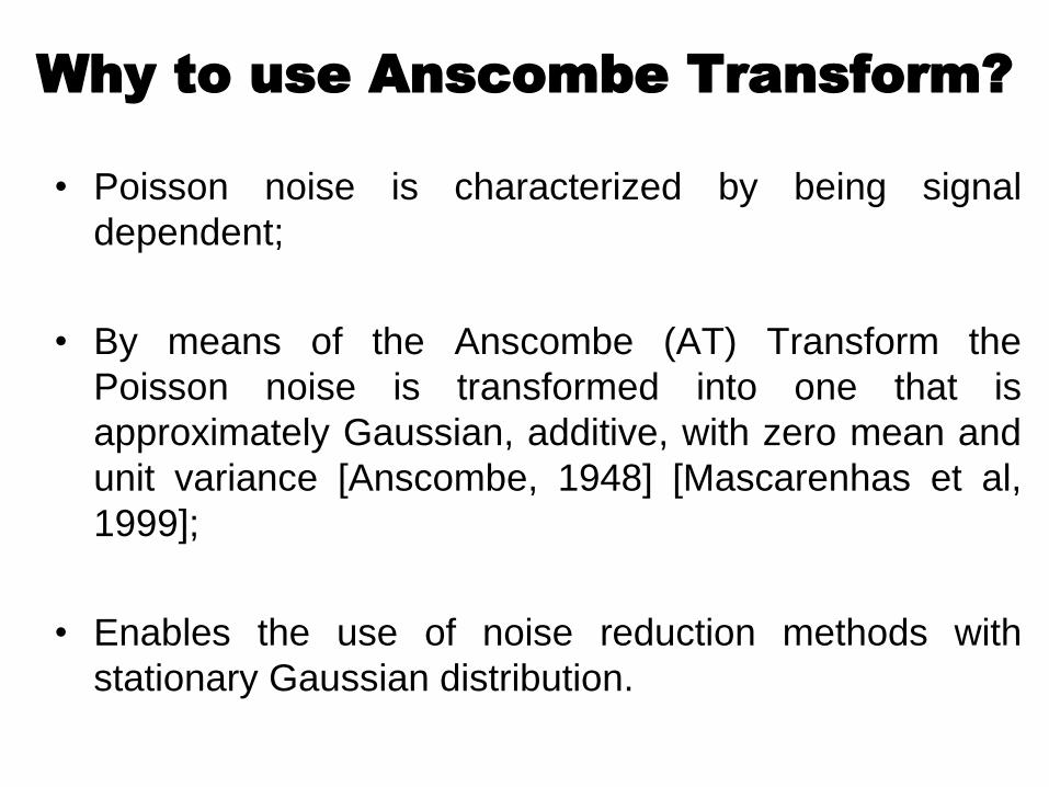
Why to use Anscombe Transform?

• Poisson noise is characterized by being signal

dependent;

• By means of the Anscombe (AT) Transform the

Poisson noise is transformed into one that is

approximately Gaussian, additive, with zero mean and

unit variance [Anscombe, 1948] [Mascarenhas et al,

1999];

• Enables the use of noise reduction methods with

stationary Gaussian distribution.

• For the random variable x (Poisson distribution) its AT will

be defined as:

8

32 ii xy

iii vxy 8

12

is

Approximately independent

Filtering Prior to Image

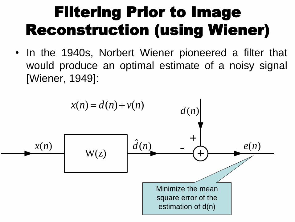
Reconstruction (using Wiener)

• In the 1940s, Norbert Wiener pioneered a filter that

would produce an optimal estimate of a noisy signal

[Wiener, 1949]:

W(z))(ˆ nd)(nx

)(nd

)(ne+

-+

)()()( nvndnx

Minimize the mean

square error of the

estimation of d(n)

Filtering Prior to Image

Reconstruction (using Wiener-FIR)

• For a FIR filtering, one may have the systems of

Wiener-Hopf equations given by:

)1(

)1(

)0(

)1(

)1(

)0(

)0()2()1(

)2()0()1(

)1()1()0(

pr

r

r

pw

w

w

rprpr

prrr

prrr

dx

dx

dx

xxx

xxx

xxx

Autocorrelation of the signal

Weights for the

FIR filter

Cross-correlation

between the desired

signal d(n)

and the input x(n)

Wiener Filtering by Linear Prediction

• From observations without noise it is sought to

estimate the value of in terms of a linear

combination of p values prior to

)1(ˆ nx)1( nx

p values

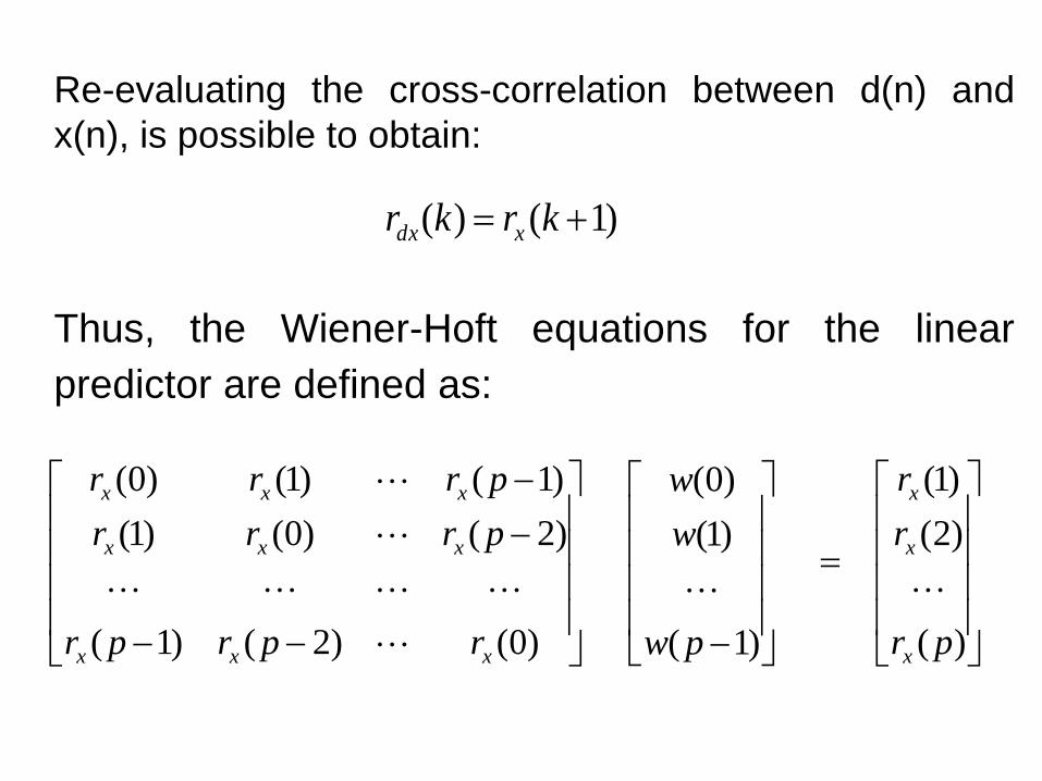
Re-evaluating the cross-correlation between d(n) and

x(n), is possible to obtain:

Thus, the Wiener-Hoft equations for the linear

predictor are defined as:

)1()( krkr xdx

)(

)2(

)1(

)1(

)1(

)0(

)0()2()1(

)2()0()1(

)1()1()0(

pr

r

r

pw

w

w

rprpr

prrr

prrr

x

x

x

xxx

xxx

xxx

3D Reconstruction for Agricultural

Soil Samples

• Tomographic data are acquired without displacement of the sample under analysis. The position during the scanning process remains the same;

• Completion of the intervals between acquisition plans (A) and virtual plans (V);

• This feature allows to use interpolation and to increase resolution of 3D objects, i.e., called as Volumetric Reconstruction

A

V

Aligned pixels used

In the process of interpolation

3D Reconstruction of Agricultural Samples - B-

Spline-Wavelet Interpolation

• Function for interpolation

N

i

i iNuBauf0

)()(

x

xx

xxx

xxx

xx

xB

20

2126

1

102646

1

012646

1

1226

1

3

32

32

3

Where u represents the

step in interpolation and N

is the number of known

points

Blending

Function

3D CT Image Reconstruction

(interpolation procedures)

Pix

el

valu

es

Slices

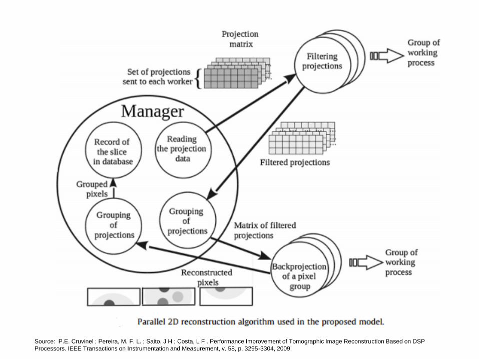
Source: P.E. Cruvinel ; Pereira, M. F. L. ; Saito, J H ; Costa, L F . Performance Improvement of Tomographic Image Reconstruction Based on DSP

Processors. IEEE Transactions on Instrumentation and Measurement, v. 58, p. 3295-3304, 2009.

Modeling the parallel algorithm for 2D and 3D

reconstruction - Mapping in DSP platform

– Interface between PC and DSP modules

– Interconnection of a network of modules

Source: Hunt Engineering Source: Xilinx Virtex

Filtering with Wiener

• Assays performed with additive Gaussian noise and

evaluation based on the resulting variance before and

after the filtration;

• In the study, a homogeneous phantom and a

heterogeneous phantom were used;

Source: M.F.L. Pereira, P.E. Cruvinel . A model for soil computed tomography based on volumetric reconstruction, Wiener filtering and parallel

processing. Computers and Electronics in Agriculture 111 (2015) 151–163.

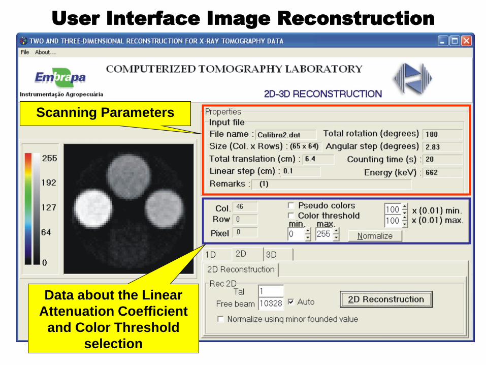
Scanning Parameters

Data about the Linear

Attenuation Coefficient

and Color Threshold

selection

User Interface Image Reconstruction

Navigate between the

Folders to select the

slices

Choice of the slices in

the range of interesting

Opening the slices for

visualization

User Interface for 3D Image Visualization

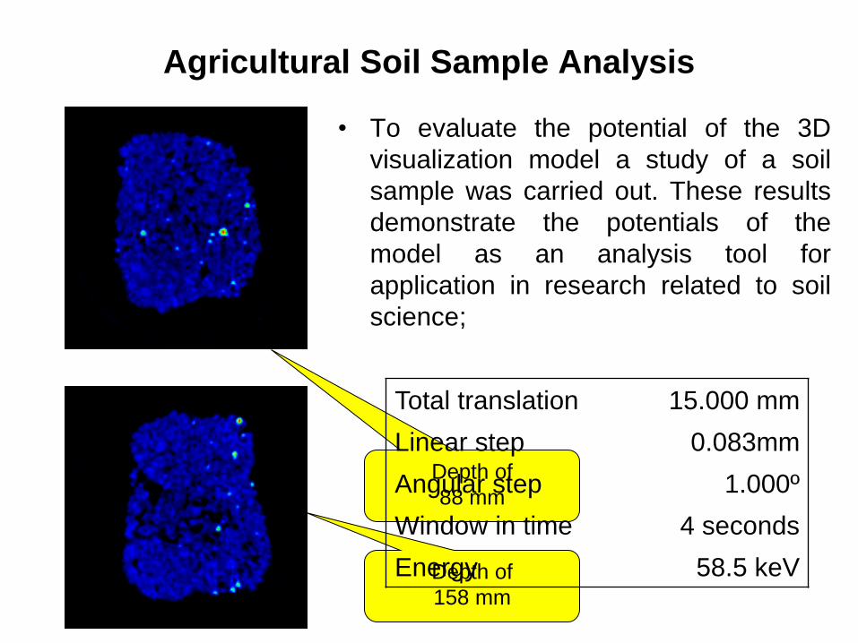
• To evaluate the potential of the 3D

visualization model a study of a soil

sample was carried out. These results

demonstrate the potentials of the

model as an analysis tool for

application in research related to soil

science;

Depth of

88 mm

Depth of

158 mm

Total translation 15.000 mm

Linear step 0.083mm

Angular step 1.000º

Window in time 4 seconds

Energy 58.5 keV

Agricultural Soil Sample Analysis

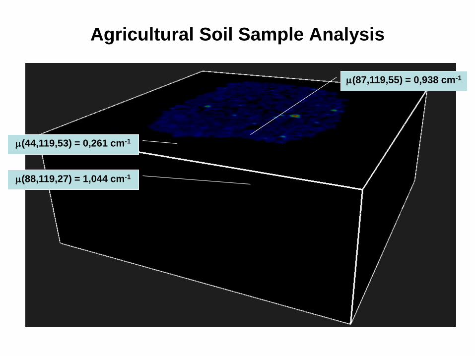
(88,119,27) = 1,044 cm-1

(44,119,53) = 0,261 cm-1

(87,119,55) = 0,938 cm-1

Agricultural Soil Sample Analysis

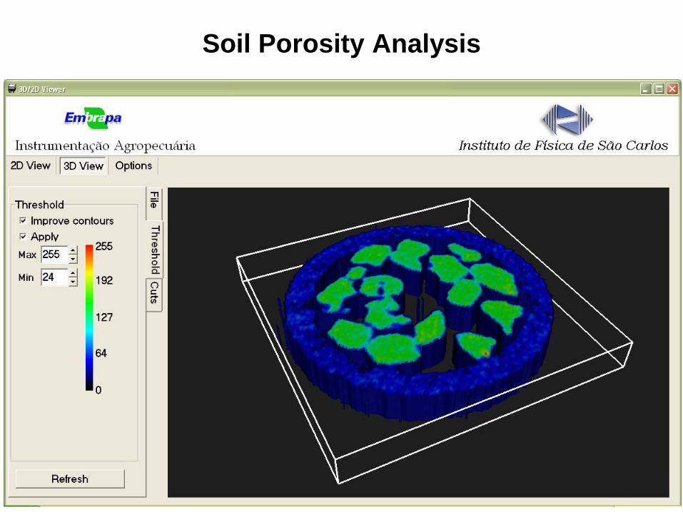
Soil Porosity Analysis

CT in Agriculture

Source: http://bruker-microct.com/applications/wood/wood002.htm

Acknowledgements

Reinaldo Dias Ferraz de Souza rferraz@mct.gov.br www.mct.gov.br

Thank You!