Journal of Computer Graphics Techniques Vol. 7, No. 2, 2018 http://jcgt.org

Cube-to-sphere Projections for ProceduralTexturing and Beyond

Matt Zucker and Yosuke HigashiSwarthmore College

(a) (b)

(c) (d)

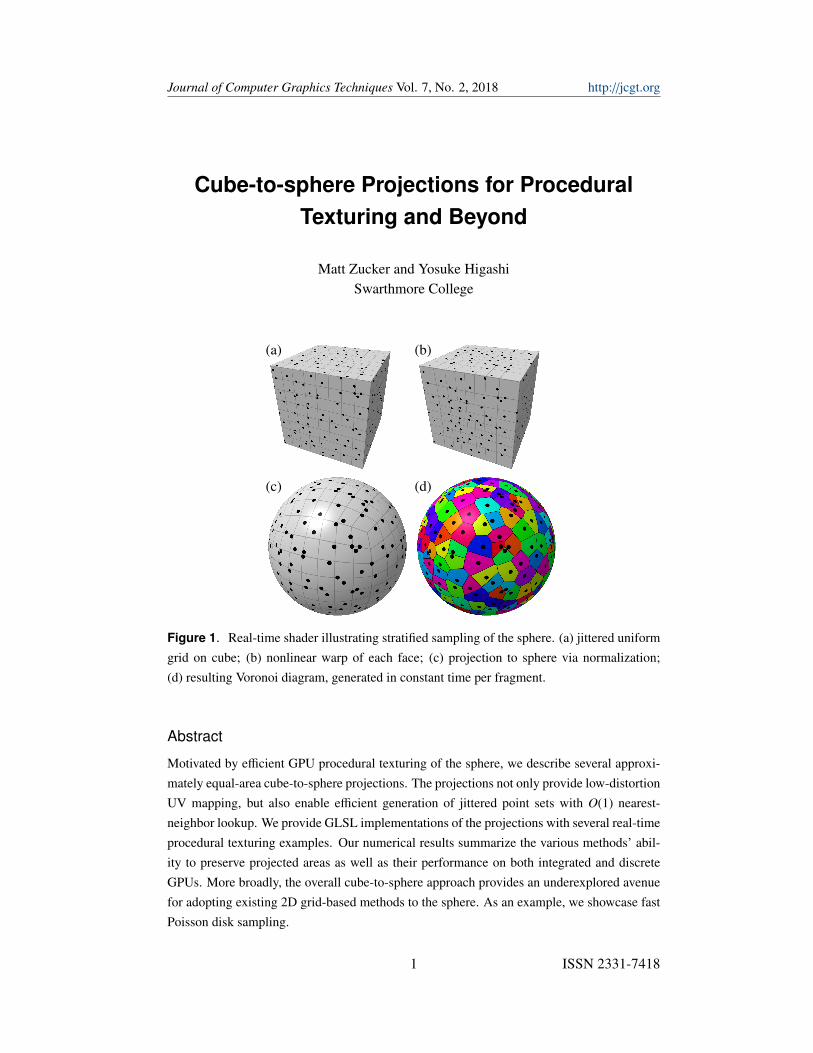
Figure 1. Real-time shader illustrating stratified sampling of the sphere. (a) jittered uniformgrid on cube; (b) nonlinear warp of each face; (c) projection to sphere via normalization;(d) resulting Voronoi diagram, generated in constant time per fragment.

Abstract

Motivated by efficient GPU procedural texturing of the sphere, we describe several approxi-mately equal-area cube-to-sphere projections. The projections not only provide low-distortionUV mapping, but also enable efficient generation of jittered point sets with O(1) nearest-neighbor lookup. We provide GLSL implementations of the projections with several real-timeprocedural texturing examples. Our numerical results summarize the various methods’ abil-ity to preserve projected areas as well as their performance on both integrated and discreteGPUs. More broadly, the overall cube-to-sphere approach provides an underexplored avenuefor adopting existing 2D grid-based methods to the sphere. As an example, we showcase fastPoisson disk sampling.

1 ISSN 2331-7418

Journal of Computer Graphics TechniquesCube-to-sphere Projections for Procedural Texturing and Beyond

Vol. 7, No. 2, 2018http://jcgt.org

1. Introduction

Spheres are ubiquitous primitives in computer graphics, used to render everythingfrom molecules to planets. Sampling and tessellating the sphere is fundamental totexturing and modeling these common objects. Most users of modern graphics APIsare familiar with cube mapping [Greene 1986], a technique that is commonly used tomap between 3D direction vectors and 2D textures tiling the surface of a cube. In thispaper, we present a family of invertible mappings that can be considered as a general-ization of cube mapping. When constructed to preserve relative area, these mappingsare useful for sampling the sphere and have applications to procedural texturing andmodeling.

1.1. Related Work

Like the spherical Fibonacci (SF) mapping of Keinert et al. [2015], the methods pre-sented here can be used to generate well-dispersed sets of points on the sphere withefficient nearest-neighbor lookup, suitable for many Voronoi-based texturing tech-niques. However, compared with SF mapping, graphics programmers and artists mayprefer to use the sphered-cube approach we describe, because it allows many existingtechniques developed for 2D Cartesian grids to be adapted to the sphere.

Although our primary motivation is GPU-based procedural texturing of spheres,the methods we study are closely related to sampling methods used for rendering,especially determining illumination. Arvo [1995] demonstrated an approach for strat-ified sampling of spherical triangles and general 2-manifolds [2001]. Others haveused cylindrical projection to create equal-area maps from plane to sphere [Shao andBadler 1996; Wong et al. 1997]. However, the resulting singularities prevent efficientnearest-neighbor search (Section 4.2) on jittered grids. We show that the sphered-cube approach can be used to generate blue-noise samples on the sphere, which canlead to higher-quality Monte Carlo estimates of spherical integrals [Singh 2015].

In contrast to other 2D representations of the sphere, such as octahedron normalvectors [Meyer et al. 2010] or HEALPix [Gorski et al. 2005], the chief advantage ofthe approach we present is that it allows straightforward application of techniquesdesigned for 2D Cartesian grids. In general, our analysis comes at a time whenthe computer graphics community is showing a renewed interest in the mathemat-ics of map projections [Lambers 2016] and novel applications of re-parameterizingthe sphere [Heitz et al. 2016].

The area-preserving cube-to-sphere projections we describe have been of particu-lar interest to other researchers in recent years [Everitt 2016; Brown 2017]. Althoughthis approach dates back over four decades [Chan and O’Neill 1975], it nonethe-less remains an underexplored method in computer graphics for adapting a broaderrange of grid-based techniques to spherical domains. Beyond the in-depth analysisand quantitative comparison we provide, our main contributions are to optimize free

2

Journal of Computer Graphics TechniquesCube-to-sphere Projections for Procedural Texturing and Beyond

Vol. 7, No. 2, 2018http://jcgt.org

parameters for previously published projections that had been chosen ad hoc and toincrease the visibility of the overall cube-to-sphere approach. We also introduce anew method: the 1D odd-polynomial projection.

1.2. Organization of this Article

The remainder of this paper is structured as follows: we begin in Section 2 by re-viewing several familiar procedural texturing primitives along with requirements fortheir implementation on spherical domains. Sections 3 and 4 derive the projectionsthat enable the sphered-cube approach and demonstrate how it satisfies these require-ments. Section 5 provides a thorough comparison of the mappings we present, aswell as our recommendations on their suggested use. Finally, Section 6 showcasesfast generation of spherical Poisson disk (blue noise) point sets as a concrete exampleof adapting other existing 2D grid-based methods using the sphered-cube approach.

2. GPU-based Procedural Texturing of the Sphere

In this section, we summarize several familiar 2D procedural texturing primitives anddiscuss both speed and quality requirements for implementing these primitives onspherical domains using the GPU. Subsequent sections will construct our sphered-cube approach to meet these requirements.

2.1. Procedural Texturing Primitives and Their Rquirements

Perhaps the most well-known procedural texturing primitive is value noise, wherecontinuous intensities are randomly assigned to points on a regular lattice. Nearby in-tensities are computed by applying a reconstruction kernel to surrounding grid points,typically a cubic Hermite spline or similar function. Whereas value noise utilizes aregular lattice of points, cellular texturing (a.k.a. Worley [1996] noise) uses pointssampled from an irregular distribution. Cellular texturing may simply assign everytexel the random color of its nearest sample point, or smoothly modulate colors basedupon the distances to the closest k points. Recently, Quılez [2015] proposed a general-ization of both primitives dubbed Voronoise. Regardless of the underlying domain—2D plane, sphere, or other smooth manifold—all three procedural texturing primitiveswe just described collectively share some fundamental requirements:

(i) Equidistributed sample points – the implementation must be able to rapidlygenerate discrete sets of evenly spaced sample points of a desired density.

(ii) Jittered point sets – the implementation must be able to generate visually non-uniform samples, with neither dense clumps nor large empty regions. Thiscan be accomplished via stratified sampling (a.k.a. jittered grids) in which thedomain is partitioned into regular subdomains of equal area which are thensampled uniformly.

3

Journal of Computer Graphics TechniquesCube-to-sphere Projections for Procedural Texturing and Beyond

Vol. 7, No. 2, 2018http://jcgt.org

(iii) Efficient nearest sample search – the implementation must be able to quicklydetermine the closest k sample points to any arbitrary point in the domain, irre-spective of the total number of sample points.

Of these, value noise requires (i) and (iii), and the other primitives require (ii) and (iii).

2.2. Spherical Domains & Comparisons to Previous Approaches

For 2D planar domains, the requirements listed above are typically met by using uni-form or jittered grids. The methods we describe in Sections 3 and 4 facilitate their useon the sphere while avoiding artifacts and other shortcomings of previous approaches.

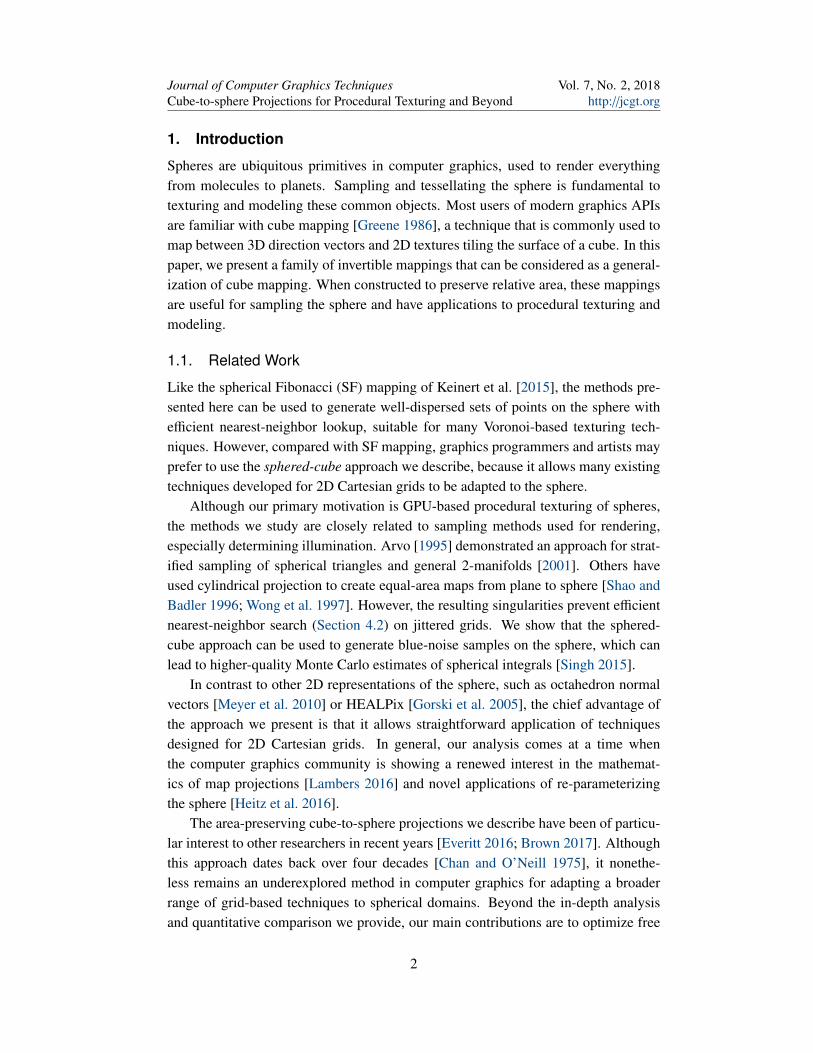
Keinert et al. [2015] show how to implement value noise with their sphericalFibonacci mapping. Their approach requires special-case code to identify the set ofbracketing points at the poles, and the resulting texture is anisotropic in these regions.

Figure 2. Real-time fragment shader generating value noise on both a uniform (left) andjittered (right) grid with m = 16 points per cube face edge.

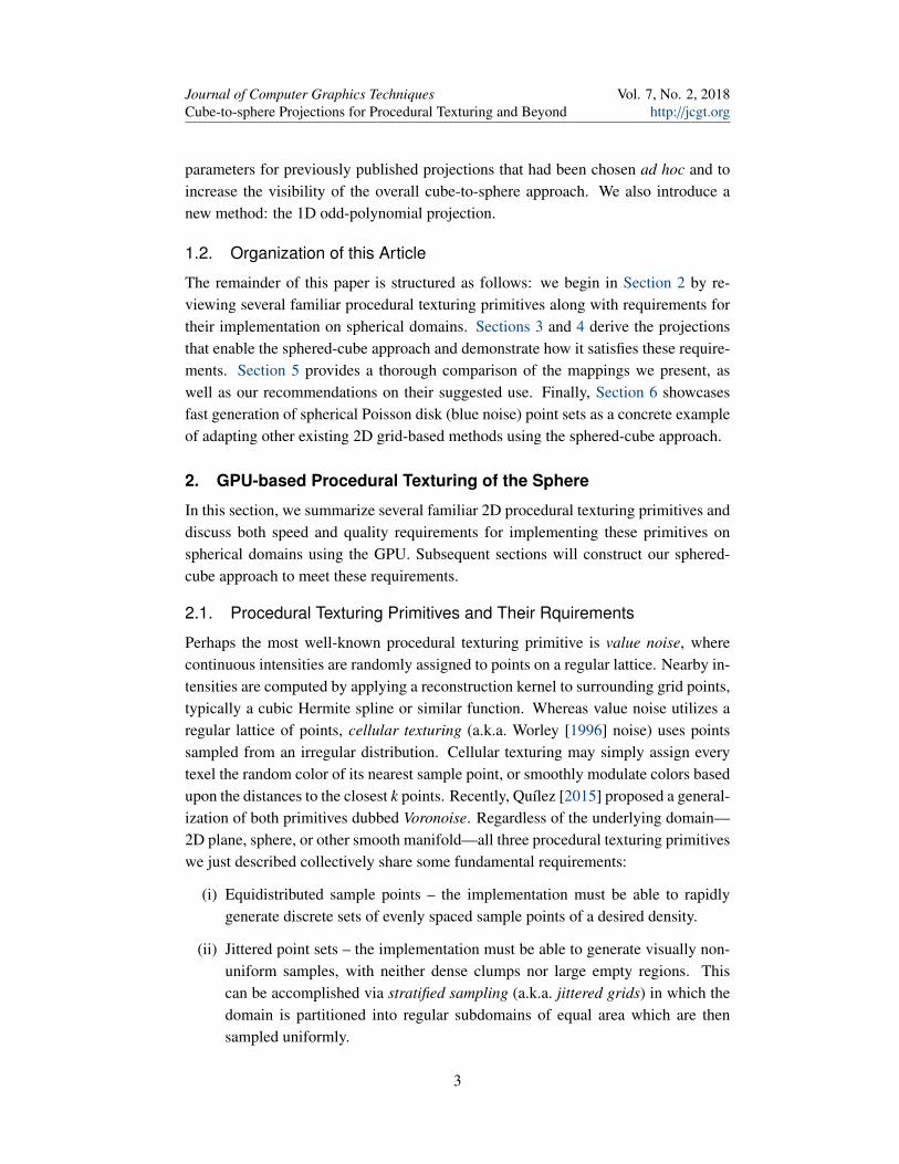
Figure 3. Real-time fragment shader comparing two types of Voronoi cells. Left side: Pointstaken from a jittered 3D grid. Note apparent curvature of cell borders as well as high variationin region sizes on the sphere. Right side: Points from jittered 2D grid on the sphered cube.3D grid based on MIT-licensed code© Inigo Quılez [2013].

4

Journal of Computer Graphics TechniquesCube-to-sphere Projections for Procedural Texturing and Beyond

Vol. 7, No. 2, 2018http://jcgt.org

(a) (b)

(c) (d)

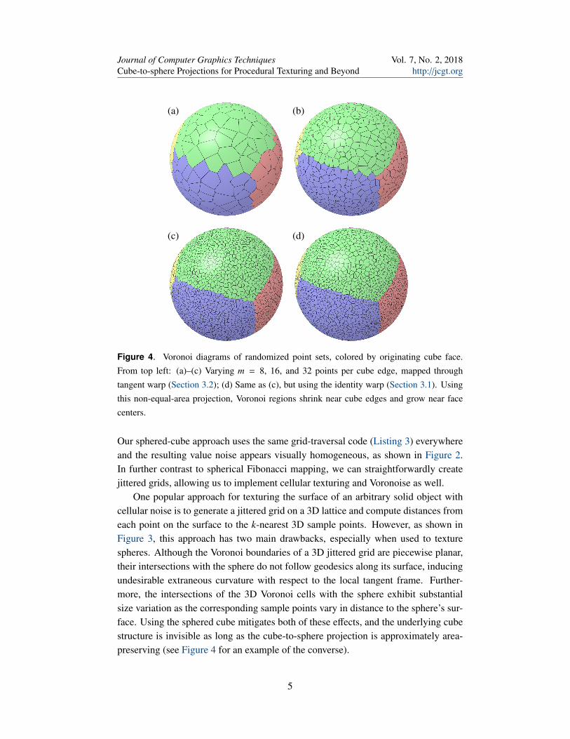
Figure 4. Voronoi diagrams of randomized point sets, colored by originating cube face.From top left: (a)–(c) Varying m = 8, 16, and 32 points per cube edge, mapped throughtangent warp (Section 3.2); (d) Same as (c), but using the identity warp (Section 3.1). Usingthis non-equal-area projection, Voronoi regions shrink near cube edges and grow near facecenters.

Our sphered-cube approach uses the same grid-traversal code (Listing 3) everywhereand the resulting value noise appears visually homogeneous, as shown in Figure 2.In further contrast to spherical Fibonacci mapping, we can straightforwardly createjittered grids, allowing us to implement cellular texturing and Voronoise as well.

One popular approach for texturing the surface of an arbitrary solid object withcellular noise is to generate a jittered grid on a 3D lattice and compute distances fromeach point on the surface to the k-nearest 3D sample points. However, as shown inFigure 3, this approach has two main drawbacks, especially when used to texturespheres. Although the Voronoi boundaries of a 3D jittered grid are piecewise planar,their intersections with the sphere do not follow geodesics along its surface, inducingundesirable extraneous curvature with respect to the local tangent frame. Further-more, the intersections of the 3D Voronoi cells with the sphere exhibit substantialsize variation as the corresponding sample points vary in distance to the sphere’s sur-face. Using the sphered cube mitigates both of these effects, and the underlying cubestructure is invisible as long as the cube-to-sphere projection is approximately area-preserving (see Figure 4 for an example of the converse).

5

Journal of Computer Graphics TechniquesCube-to-sphere Projections for Procedural Texturing and Beyond

Vol. 7, No. 2, 2018http://jcgt.org

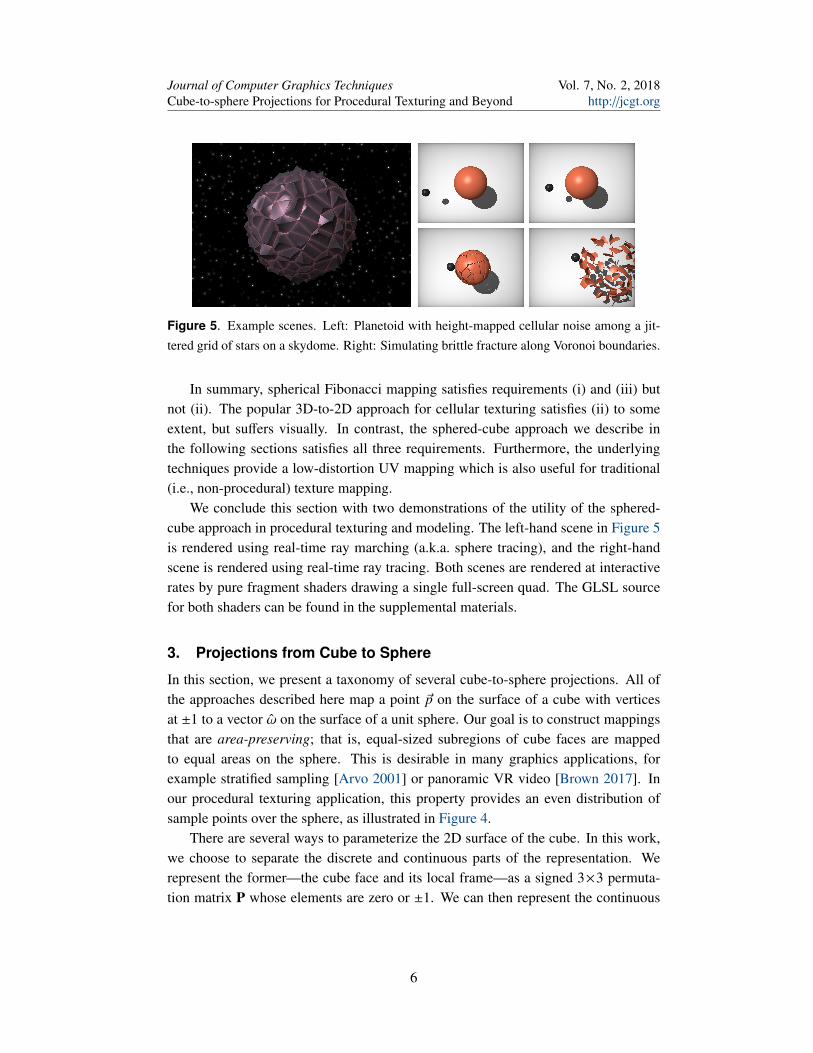
Figure 5. Example scenes. Left: Planetoid with height-mapped cellular noise among a jit-tered grid of stars on a skydome. Right: Simulating brittle fracture along Voronoi boundaries.

In summary, spherical Fibonacci mapping satisfies requirements (i) and (iii) butnot (ii). The popular 3D-to-2D approach for cellular texturing satisfies (ii) to someextent, but suffers visually. In contrast, the sphered-cube approach we describe inthe following sections satisfies all three requirements. Furthermore, the underlyingtechniques provide a low-distortion UV mapping which is also useful for traditional(i.e., non-procedural) texture mapping.

We conclude this section with two demonstrations of the utility of the sphered-cube approach in procedural texturing and modeling. The left-hand scene in Figure 5is rendered using real-time ray marching (a.k.a. sphere tracing), and the right-handscene is rendered using real-time ray tracing. Both scenes are rendered at interactiverates by pure fragment shaders drawing a single full-screen quad. The GLSL sourcefor both shaders can be found in the supplemental materials.

3. Projections from Cube to Sphere

In this section, we present a taxonomy of several cube-to-sphere projections. All ofthe approaches described here map a point ~p on the surface of a cube with verticesat ±1 to a vector ω on the surface of a unit sphere. Our goal is to construct mappingsthat are area-preserving; that is, equal-sized subregions of cube faces are mappedto equal areas on the sphere. This is desirable in many graphics applications, forexample stratified sampling [Arvo 2001] or panoramic VR video [Brown 2017]. Inour procedural texturing application, this property provides an even distribution ofsample points over the sphere, as illustrated in Figure 4.

There are several ways to parameterize the 2D surface of the cube. In this work,we choose to separate the discrete and continuous parts of the representation. Werepresent the former—the cube face and its local frame—as a signed 3×3 permuta-tion matrix P whose elements are zero or ±1. We can then represent the continuous

6

Journal of Computer Graphics TechniquesCube-to-sphere Projections for Procedural Texturing and Beyond

Vol. 7, No. 2, 2018http://jcgt.org

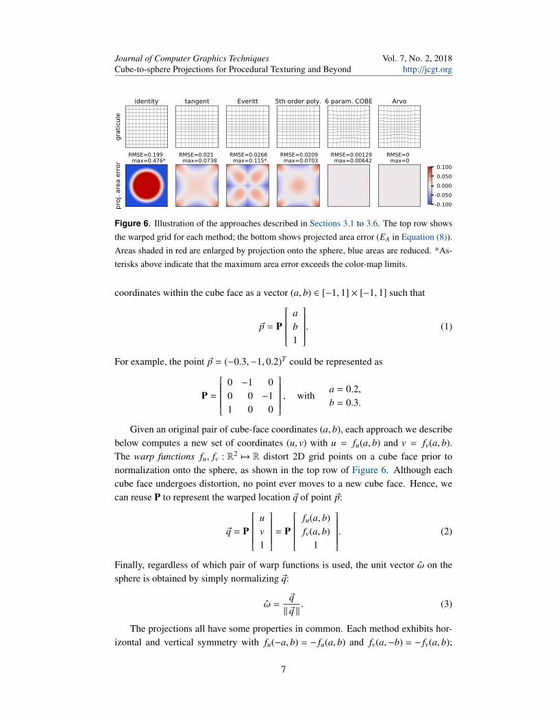
Figure 6. Illustration of the approaches described in Sections 3.1 to 3.6. The top row showsthe warped grid for each method; the bottom shows projected area error (EA in Equation (8)).Areas shaded in red are enlarged by projection onto the sphere, blue areas are reduced. *As-terisks above indicate that the maximum area error exceeds the color-map limits.

coordinates within the cube face as a vector (a, b) ∈ [−1, 1] × [−1, 1] such that

~p = P

ab1

. (1)

For example, the point ~p = (−0.3,−1, 0.2)T could be represented as

P =

0 −1 00 0 −11 0 0

, witha = 0.2,b = 0.3.

Given an original pair of cube-face coordinates (a, b), each approach we describebelow computes a new set of coordinates (u, v) with u = fu(a, b) and v = fv(a, b).The warp functions fu, fv : R2 7→ R distort 2D grid points on a cube face prior tonormalization onto the sphere, as shown in the top row of Figure 6. Although eachcube face undergoes distortion, no point ever moves to a new cube face. Hence, wecan reuse P to represent the warped location ~q of point ~p:

~q = P

uv1

= P

fu(a, b)fv(a, b)

1

. (2)

Finally, regardless of which pair of warp functions is used, the unit vector ω on thesphere is obtained by simply normalizing ~q:

ω =~q‖ ~q ‖

. (3)

The projections all have some properties in common. Each method exhibits hor-izontal and vertical symmetry with fu(−a, b) = − fu(a, b) and fv(a,−b) = − fv(a, b);

7

Journal of Computer Graphics TechniquesCube-to-sphere Projections for Procedural Texturing and Beyond

Vol. 7, No. 2, 2018http://jcgt.org

therefore, fu(0, b) = fv(a, 0) = 0 and so the center of the cube face is not displaced.Furthermore, the edges of the cube face are not displaced, so fu(1, b) = fv(a, 1) = 1.However, the approaches differ in several key qualitative aspects. Each one may be:

• bivariate (the general case), or univariate if there exists a function f : R 7→ Rwith fu(a, b) = f (a) and fv(a, b) = f (b);

• diagonally symmetric with fu(a, b) = fv(b, a); i.e., the warp treats the parame-ters a and b interchangeably. All univariate warps are diagonally symmetric;

• analytically invertible or only approximately invertible via numerical root find-ing (we discuss this in detail in Section 4).

Aside from these key categorical distinctions, the most important quantitative differ-ence between the approaches described here is the degree to which they are area-preserving; that is, a region covering a given percentage of the unit cube covers thesame percentage of the unit sphere after transformation.

Here we follow Arvo’s [2001] recipe for deriving the area element of the transfor-mation defined by the composition of Equations (1) to (3). According to the methodhe provides, the area element is given by

dA(a, b) =

√(∂ω

∂a·∂ω

∂a

) (∂ω

∂b·∂ω

∂b

)−

(∂ω

∂a·∂ω

∂b

)2

, (4)

where ∂ω∂a and ∂ω

∂b are the partial derivatives of the unit vector ω with respect to theinput cube face coordinates a and b. They are defined as

∂ω

∂a=

1(u2 + v2 + 1

) 32

−uv∂ fv

∂a + v2 ∂ fu∂a +

∂ fu∂a

u2 ∂ fv∂a − uv∂ fu

∂a +∂ fv∂a

−u∂ fu∂a − v∂ fv

∂a

, (5)

and∂ω

∂b=

1(u2 + v2 + 1

) 32

−uv∂ fv

∂b + v2 ∂ fu∂b +

∂ fu∂b

u2 ∂ fv∂b − uv∂ fu

∂b +∂ fv∂b

−u∂ fu∂b − v∂ fv

∂b

. (6)

Substituting these definitions into Equation (4) and simplifying, we obtain

dA(a, b) =

[∂ fu∂a

∂ fv∂b−∂ fu∂b

∂ fv∂a

] (u2 + v2 + 1

)− 32 . (7)

For an exact equal-area cube-to-sphere mapping, dA(a, b) is equal to π6 everywhere.

However, if the mapping is not equal-area, we may choose its free parameters tominimize the root-mean-squared error of the area element on a grid of (a, b) samples:

RMSE =

√√1n

n∑i=1

EA(ai, bi)2 , (8)

8

Journal of Computer Graphics TechniquesCube-to-sphere Projections for Procedural Texturing and Beyond

Vol. 7, No. 2, 2018http://jcgt.org

where EA(a, b) = dA(a, b) − π6 . This optimization scheme was used previously by

Chan and O’Neill [1975]; one contribution of our work is to apply it to a numberof approaches whose parameters were not previously chosen optimally. For each ofthe warping approaches described below with free parameters to optimize, we mini-mize Equation (8) over a uniform grid of 256×256 samples covering the [0, 1] rangeof (a, b). See Table 1 for a summary of the numerical optimization results and Table 3for optimal values of the free parameters. GLSL implementations of all mappings andtheir inverses can be found among the supplemental materials.

3.1. Identity Function (Standard Cube Maps)

The most straightforward projection from the cube to the sphere sets u = a and v = b.Although this mapping exhibits the largest area error of all of the approaches de-scribed here, many graphics programmers are familiar with this approach as it formsthe basis of standard cube maps [Greene 1986].

3.2. Tangent Warp Function

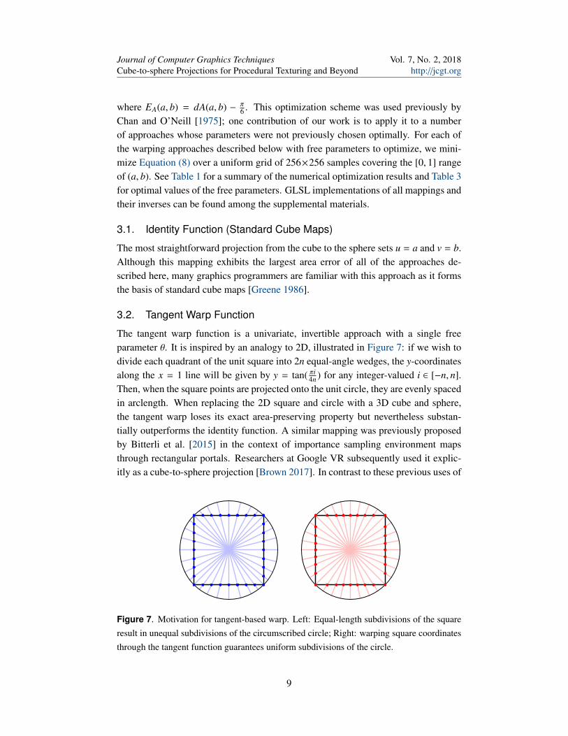
The tangent warp function is a univariate, invertible approach with a single freeparameter θ. It is inspired by an analogy to 2D, illustrated in Figure 7: if we wish todivide each quadrant of the unit square into 2n equal-angle wedges, the y-coordinatesalong the x = 1 line will be given by y = tan( πi

4n ) for any integer-valued i ∈ [−n, n].Then, when the square points are projected onto the unit circle, they are evenly spacedin arclength. When replacing the 2D square and circle with a 3D cube and sphere,the tangent warp loses its exact area-preserving property but nevertheless substan-tially outperforms the identity function. A similar mapping was previously proposedby Bitterli et al. [2015] in the context of importance sampling environment mapsthrough rectangular portals. Researchers at Google VR subsequently used it explic-itly as a cube-to-sphere projection [Brown 2017]. In contrast to these previous uses of

Figure 7. Motivation for tangent-based warp. Left: Equal-length subdivisions of the squareresult in unequal subdivisions of the circumscribed circle; Right: warping square coordinatesthrough the tangent function guarantees uniform subdivisions of the circle.

9

Journal of Computer Graphics TechniquesCube-to-sphere Projections for Procedural Texturing and Beyond

Vol. 7, No. 2, 2018http://jcgt.org

the tangent mapping, our implementation introduces and optimizes a free parameterto better preserve area.

The free parameter is implicitly fixed at π4 by both of the works we just cited,

and this value is indeed optimal for equalizing angles in the 2D motivating example.However, in 3D it is possible to preserve area more effectively by using the warp

u = f (a) =tan(aθ)tan(θ)

(9)

for some angle θ > 0. The inverse of the tangent warp is given by

a = f −1(u) =1θ

tan−1 (u tan(θ)

). (10)

3.3. Everitt’s Univariate Invertible Warp Function

Everitt [2014] proposed a univariate, invertible warp function and a subsequent re-finement [2016] whose respective formulas are

f (a) = sgn(a)(

32 −

12

√9 − 8 |a|

), (11)

and f (a) = sgn(a)(

116 −

16

√121 − 96 |a|

). (12)

The general warp is best understood by considering its piecewise-quadratic inverse

a = f −1(u) = u(ε + (1 − ε) |u|

)(13)

for some ε > 1. Upon inspection, f −1(1) = 1, and f −1(−u) = − f −1(u). To obtain theforward warp function we solve for u and find

u = f (a) = sgn(a)

ε − √ε2 − 4 (ε − 1) |a|2(ε − 1)

. (14)

Everitt’s Equation (11) is a special case of Equation (14) with ε = 1.5, and Equa-tion (12) sets ε = 1.375.

3.4. Odd 1D polynomial

To finish off the univariate methods, we introduce the odd (antisymmetric) polynomial

f (a) = k1a + k2a3 + k3a5 + . . . (15)

By construction, f (−a) = − f (a). An odd polynomial with n coefficients has degree2n − 1, and to enforce the constraint that f (1) = 1, we require that

∑ni=1 ki = 1.

The inspiration for our design of this method is that trigonometric functions, par-ticularly inverse functions, can be expensive to evaluate and are hence frequentlyreplaced by polynomial approximations. In this case, instead of optimizing polyno-mial coefficients to approximate tan(x) as closely as possible, we directly optimizethe coefficients to minimize Equation (8). Indeed, the polynomials obtained throughoptimization visually resemble the tangent function. However, unlike the tangent andEveritt approaches, they are not analytically invertible for n > 2.

10

Journal of Computer Graphics TechniquesCube-to-sphere Projections for Procedural Texturing and Beyond

Vol. 7, No. 2, 2018http://jcgt.org

3.5. COBE Quadrilateralized Spherical Cube

Chan and O’Neill [1975] proposed a bivariate, diagonally symmetric polynomial

fu(a, b) = λa + (1 − λ) a3 + (1 − a2) a∞∑

(i+ j)≥1

γi j a2i b2 j. (16)

By construction, Equation (16) satisfies the requirements that fu(−a, b) = − fu(a, b),and fu(1, b) = 1. Owing to diagonal symmetry, the second cube coordinate is definedby fv(a, b) = fu(b, a). Their model is often called the COBE quadrilateralized spher-ical cube model, as it was developed in support of the NASA Cosmic BackgroundExplorer (COBE) project.

3.6. Arvo’s Exact Equal-area Method

Arvo [2001] provides a recipe for analytically constructing an area-preserving pa-rameterization between smooth 2D surfaces. We apply Arvo’s method to construct anequal-area mapping from cube face to sphere, arriving at the warp functions:

u = fu(a, b) =

√2 tan

(πa6

)√

1 − tan(πa6

)2and v = fv(a, b) =

b√1 + (1 − b2) cos

(πa3

) . (17)

Arvo’s recipe also produces an inverse mapping given by

a =6π

tan−1(

u√

u2 + 2

)and b =

v√

u2 + 2u2 + v2 + 1

. (18)

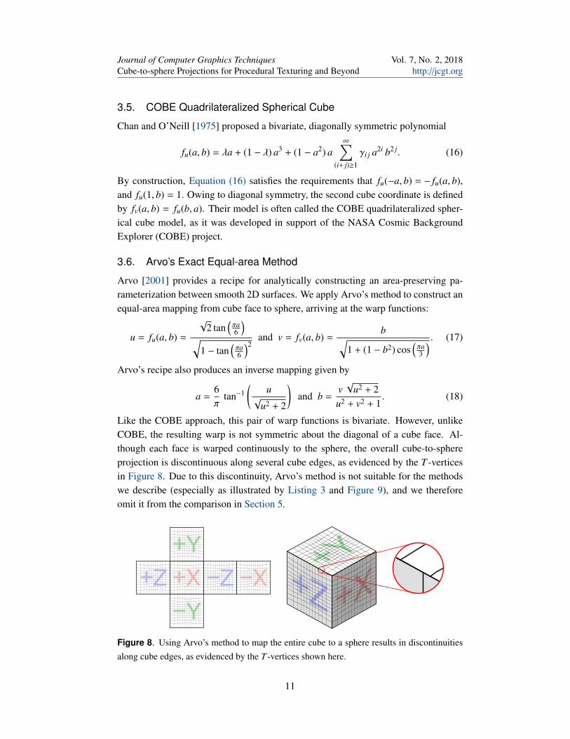
Like the COBE approach, this pair of warp functions is bivariate. However, unlikeCOBE, the resulting warp is not symmetric about the diagonal of a cube face. Al-though each face is warped continuously to the sphere, the overall cube-to-sphereprojection is discontinuous along several cube edges, as evidenced by the T -verticesin Figure 8. Due to this discontinuity, Arvo’s method is not suitable for the methodswe describe (especially as illustrated by Listing 3 and Figure 9), and we thereforeomit it from the comparison in Section 5.

Figure 8. Using Arvo’s method to map the entire cube to a sphere results in discontinuitiesalong cube edges, as evidenced by the T -vertices shown here.

11

Journal of Computer Graphics TechniquesCube-to-sphere Projections for Procedural Texturing and Beyond

Vol. 7, No. 2, 2018http://jcgt.org

4. Inverse Mappings and Nearest-neighbor Lookup

The cube-to-sphere mappings defined in Sections 3.1 to 3.5 can be used to distributesamples pseudorandomly on the surface of a sphere, as shown in Figure 1. The firststep is to generate a jittered grid of points on the cube by discretizing each face intom × m square grid cells and randomly choosing a sample within each cell. Thesesamples can then be warped and projected to the sphere via Equations (1) to (3).Given a unit vector ω, it is possible to identify the closest sample point by brute-forceiteration over all 6m2 warped and projected samples. However, a far more efficientmethod begins by first identifying the unwarped grid cell on the cube correspondingto ω.

To accomplish this, it must be possible to invert the mappings described in Sec-tion 3; that is, find the (a, b)-coordinates on a cube face that map to a given ω. Thefirst step is to project ω onto the cube, as when performing a cube-map lookup. Weidentify the coordinate with the greatest absolute value and construct an appropriatesigned permutation matrix P establishing the cube face and local coordinate system.We can then obtain the warped-cube coordinates (u, v) by computing

xyz

= PT ω (19)

and setting u = x/z and v = y/z (i.e., dividing by the value of the maximal coordinate).What remains is to invert the mapping function: given u = fu(a, b) and v = fv(a, b),solve for a and b. The inverses of the tangent warp and Everitt’s warp are given inSections 3.2 and 3.3. However, the odd 1D polynomial method (Section 3.4) and theCOBE method (Section 3.5) must be inverted numerically.

4.1. Numerical Inverses

For both the 1D polynomial and COBE warps, we begin by fitting an approximate in-verse polynomial f −1 of the same parametric form as Equation (15) or Equation (16),respectively. Each polynomial fit minimizes a sum of squared residual errors ei. Inthe case of the univariate polynomial, we choose the coefficients of f −1 to minimize

ei =∣∣∣ f −1( f (ai)

)− ai

∣∣∣ (20)

over a linearly spaced set of samples ai ∈ [0, 1]. For the bivariate polynomial, wechoose the coefficients of f −1 : R2 7→ R to minimize

ei =

∥∥∥∥∥∥ f −1(ui, vi)

f −1(vi, ui)

− ai

bi

∥∥∥∥∥∥ , withui = fu(ai, bi)vi = fv(ai, bi) = fu(bi, ai)

(21)

over a uniform grid of (ai, bi) ∈ [0, 1] × [0, 1] (note diagonal symmetry).

12

Journal of Computer Graphics TechniquesCube-to-sphere Projections for Procedural Texturing and Beyond

Vol. 7, No. 2, 2018http://jcgt.org

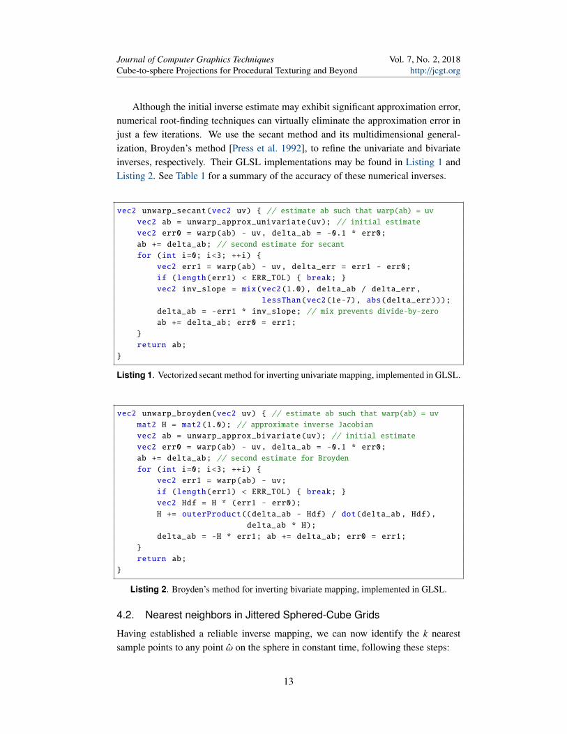
Although the initial inverse estimate may exhibit significant approximation error,numerical root-finding techniques can virtually eliminate the approximation error injust a few iterations. We use the secant method and its multidimensional general-ization, Broyden’s method [Press et al. 1992], to refine the univariate and bivariateinverses, respectively. Their GLSL implementations may be found in Listing 1 andListing 2. See Table 1 for a summary of the accuracy of these numerical inverses.

vec2 unwarp_secant(vec2 uv) { // estimate ab such that warp(ab) = uv

vec2 ab = unwarp_approx_univariate(uv); // initial estimate

vec2 err0 = warp(ab) - uv, delta_ab = -0.1 * err0;

ab += delta_ab; // second estimate for secant

for (int i=0; i<3; ++i) {

vec2 err1 = warp(ab) - uv, delta_err = err1 - err0;

if (length(err1) < ERR_TOL) { break; }

vec2 inv_slope = mix(vec2(1.0), delta_ab / delta_err ,

lessThan(vec2(1e-7), abs(delta_err)));

delta_ab = -err1 * inv_slope; // mix prevents divide-by-zero

ab += delta_ab; err0 = err1;

}

return ab;

}

Listing 1. Vectorized secant method for inverting univariate mapping, implemented in GLSL.

vec2 unwarp_broyden(vec2 uv) { // estimate ab such that warp(ab) = uv

mat2 H = mat2(1.0); // approximate inverse Jacobian

vec2 ab = unwarp_approx_bivariate(uv); // initial estimate

vec2 err0 = warp(ab) - uv, delta_ab = -0.1 * err0;

ab += delta_ab; // second estimate for Broyden

for (int i=0; i<3; ++i) {

vec2 err1 = warp(ab) - uv;

if (length(err1) < ERR_TOL) { break; }

vec2 Hdf = H * (err1 - err0);

H += outerProduct((delta_ab - Hdf) / dot(delta_ab, Hdf),

delta_ab * H);

delta_ab = -H * err1; ab += delta_ab; err0 = err1;

}

return ab;

}

Listing 2. Broyden’s method for inverting bivariate mapping, implemented in GLSL.

4.2. Nearest neighbors in Jittered Sphered-Cube Grids

Having established a reliable inverse mapping, we can now identify the k nearestsample points to any point ω on the sphere in constant time, following these steps:

13

Journal of Computer Graphics TechniquesCube-to-sphere Projections for Procedural Texturing and Beyond

Vol. 7, No. 2, 2018http://jcgt.org

1. Unproject ω to get the permutation matrix P, and use the inverse mapping toget the unwarped face coordinates (a, b).

2. Search an s × s neighborhood of grid cells (e.g., 2×2 for k = 1, or larger fork > 1, see below) to find the closest sample point(s).

3. When ranking sample points, use distance on the sphere to ω (as opposed todistance on the flat cube faces). It is sufficient to choose the sample point thathas the maximum dot product with the 3D vector ω.

The single closest sample point always lies within a 2×2 neighborhood centered onthe cell corner closest to ω. However, to correctly identify the second-closest sample,it is necessary to search a 4×4 neighborhood instead. In general, a larger k implieslarger neighborhoods. Since it does not depend on the grid size m, but only on theneighborhood size s, the algorithm outlined above runs in constant time with respectto the total number of sample points.

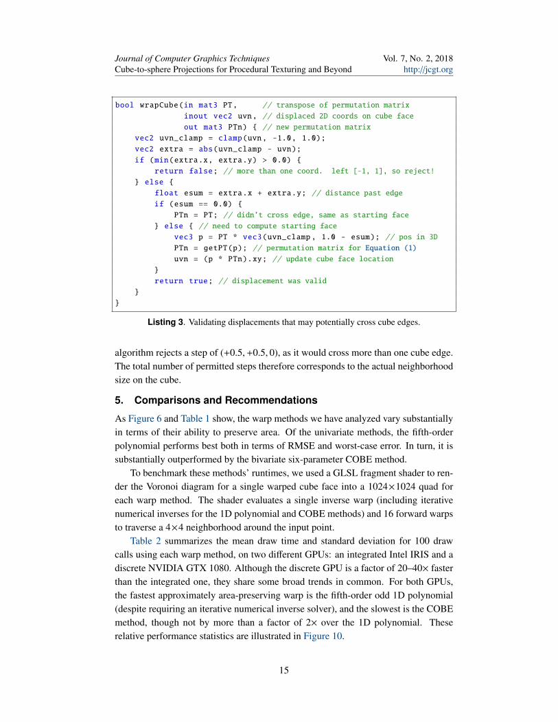
Aside from using the correct metric to rank points—distance on the sphere, asopposed to the cube—when adopting grid-based methods using the cube-to-sphereapproach, it is vital to respect edge-wrapping effects while iterating over neighbor-hoods. For example, a 3×3 neighborhood is the set of grid cells on the cube that canbe accessed by moving up one step in the horizontal and vertical directions from thecenter cell. Although in the 2D planar domain this always results in a neighborhoodsize of nine cells, there may be fewer on the cube, as shown in Figure 9.

We address this issue with an algorithm (Listing 3) that handles edge wrappingand rejects steps (e.g., offsets to neighboring cells) that would cross more than onecube edge. With respect to the central point at (0.75, 0.75, 1) in Figure 9, the algo-rithm permits a step of (+0.5, 0, 0), causing a wrap across to the positive-x face of thecube, or a step of (0,+0.5, 0) that wraps across to the positive-y face. However, the

x

y

z

0.750.25

−0.25−0.75

−0.75

−0.25

0.25

0.75

−0.75−0.25

0.250.75

Figure 9. On the cube, considering all cells within ±1 horizontal or vertical steps of a centralcell may result in fewer neighbors than would be found on a 2D planar grid.

14

Journal of Computer Graphics TechniquesCube-to-sphere Projections for Procedural Texturing and Beyond

Vol. 7, No. 2, 2018http://jcgt.org

bool wrapCube(in mat3 PT, // transpose of permutation matrix

inout vec2 uvn, // displaced 2D coords on cube face

out mat3 PTn) { // new permutation matrix

vec2 uvn_clamp = clamp(uvn, -1.0, 1.0);

vec2 extra = abs(uvn_clamp - uvn);

if (min(extra.x, extra.y) > 0.0) {

return false; // more than one coord. left [-1, 1], so reject!

} else {

float esum = extra.x + extra.y; // distance past edge

if (esum == 0.0) {

PTn = PT; // didn’t cross edge, same as starting face

} else { // need to compute starting face

vec3 p = PT * vec3(uvn_clamp , 1.0 - esum); // pos in 3D

PTn = getPT(p); // permutation matrix for Equation (1)

uvn = (p * PTn).xy; // update cube face location

}

return true; // displacement was valid

}

}

Listing 3. Validating displacements that may potentially cross cube edges.

algorithm rejects a step of (+0.5,+0.5, 0), as it would cross more than one cube edge.The total number of permitted steps therefore corresponds to the actual neighborhoodsize on the cube.

5. Comparisons and Recommendations

As Figure 6 and Table 1 show, the warp methods we have analyzed vary substantiallyin terms of their ability to preserve area. Of the univariate methods, the fifth-orderpolynomial performs best both in terms of RMSE and worst-case error. In turn, it issubstantially outperformed by the bivariate six-parameter COBE method.

To benchmark these methods’ runtimes, we used a GLSL fragment shader to ren-der the Voronoi diagram for a single warped cube face into a 1024×1024 quad foreach warp method. The shader evaluates a single inverse warp (including iterativenumerical inverses for the 1D polynomial and COBE methods) and 16 forward warpsto traverse a 4×4 neighborhood around the input point.

Table 2 summarizes the mean draw time and standard deviation for 100 drawcalls using each warp method, on two different GPUs: an integrated Intel IRIS and adiscrete NVIDIA GTX 1080. Although the discrete GPU is a factor of 20–40× fasterthan the integrated one, they share some broad trends in common. For both GPUs,the fastest approximately area-preserving warp is the fifth-order odd 1D polynomial(despite requiring an iterative numerical inverse solver), and the slowest is the COBEmethod, though not by more than a factor of 2× over the 1D polynomial. Theserelative performance statistics are illustrated in Figure 10.

15

Journal of Computer Graphics TechniquesCube-to-sphere Projections for Procedural Texturing and Beyond

Vol. 7, No. 2, 2018http://jcgt.org

Parameter Area Area Initial NumericalWarp method source RMSE max error inv. error inv. erroridentity N/A 0.199 0.476 – –

tangent θ = π4 [Brown 2017] 0.047 0.0933 – –

θ ≈ 0.8687 (optimal) 0.021 0.0738 – –

Everitt ε = 1.5 [Everitt 2014] 0.0353 0.246 – –ε = 1.375 [Everitt 2016] 0.0436 0.112 – –ε ≈ 1.4511 (optimal) 0.0266 0.115 – –

5th order poly. optimal 0.0209 0.0703 0.00109 5.55 × 10−16

6 param. COBE optimal 0.0013 0.00642 0.00187 3.96 × 10−8

Table 1. Summary of numerical results for projected area error and inverse approximations.Area RMSE is the optimization objective (Equation (8)) and area max error is the worst-caseobserved value for EA in that equation. Inverse errors refer to the worst-case observed valuefor the initial inverse guess and subsequent refinement by an iterative solver. Dashes indicatethe method has an analytic inverse.

Intel IRIS NVIDIA GTX 1080Warp method mean std. mean std.identity 2.262 ms 0.056 ms 0.071 ms 0.011 mstangent 3.277 ms 0.057 ms 0.163 ms 0.006 msEveritt 2.926 ms 0.051 ms 0.178 ms 0.004 ms5th order poly. 2.846 ms 0.033 ms 0.143 ms 0.009 ms6 param. COBE 3.581 ms 0.038 ms 0.218 ms 0.006 ms

Table 2. Frame timing data collected on two different GPUs.

Figure 10. Timing data from Table 2 normalized to show trends across two different GPUs.Error bars indicate ±1 standard deviation.

16

Journal of Computer Graphics TechniquesCube-to-sphere Projections for Procedural Texturing and Beyond

Vol. 7, No. 2, 2018http://jcgt.org

Warp method/param. Forward Inversetangent θ 0.8687 –Everitt ε 1.4511 –5th order poly. k1 0.1239 0.1433

k2 0.1305 −0.4865k3 0.7456 1.3432

6 param. COBE λ 0.7240 1.3774γ10 −0.0941 −0.2129γ01 0.0276 −0.1178γ20 −0.0623 0.0694γ11 0.0409 0.0941γ02 0.0342 0.0108

Table 3. Optimal free parameters for the mappings defined in Sections 3.2 to 3.5 along withtheir approximate inverses (Section 4.1). Dashes indicate the method has an analytic inverse.

Summarizing our results: if speed is paramount, we recommend the fifth-orderodd 1D polynomial. It is also the best univariate method in terms of projected areaerror. If area-preserving capability is the chief criterion, we recommend the COBEmethod (although for our procedural texturing application, all of the methods visuallyappear nearly identical). Finally, to maximize ease of implementation, we recommendthe tangent method, as it outperforms Everitt’s method in preserving area.

6. Generalizing 2D Grid-based Methods to the Sphere

Beyond texturing, the cube-to-sphere approach enables a broader range of 2D grid-based methods to be extended to the sphere with minimal distortion. This is a particu-larly useful feature because methods on the plane that make use of an underlying gridstructure are often simple, fast, and easily parallelizable on the GPU. As an example,we extend a state-of-the-art 2D Poisson disk sampling algorithm to the spherical do-main using cube-to-sphere mapping and show that the quality of the resulting pointset is not compromised.

Poisson disk sampling generates a uniformly random set of points such that notwo are closer than a specified minimum distance. Naıve dart throwing [Cook 1986]becomes intractably slow as the number of points increases, so considerable effort hasgone into improving runtime, especially in the planar domain [Wei 2008; Gamito andMaddock 2009] as well as on arbitrary surfaces [Bowers et al. 2010; Cline et al. 2009].Comparatively little work has been done on explicitly generating Poisson disk distri-butions on a sphere. Generating the point set on a unit square and then lifting it upto the sphere using an equal-area projection preserves the point set’s asymptotic dis-tribution uniformity, but not distances between samples [Marques et al. 2013]. Otheralgorithms that directly sample on the sphere [Cline et al. 2009; Gamito and Maddock2009] are not straightforward to parallelize on the GPU.

17

Journal of Computer Graphics TechniquesCube-to-sphere Projections for Procedural Texturing and Beyond

Vol. 7, No. 2, 2018http://jcgt.org

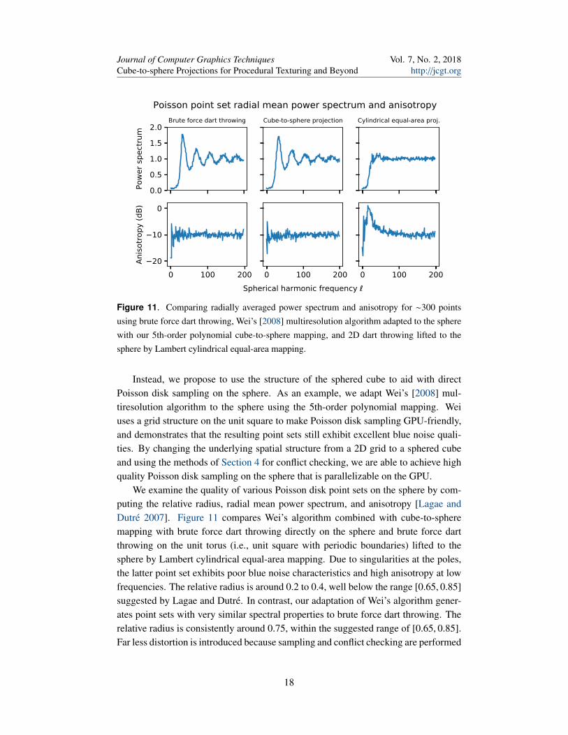
Figure 11. Comparing radially averaged power spectrum and anisotropy for ∼300 pointsusing brute force dart throwing, Wei’s [2008] multiresolution algorithm adapted to the spherewith our 5th-order polynomial cube-to-sphere mapping, and 2D dart throwing lifted to thesphere by Lambert cylindrical equal-area mapping.

Instead, we propose to use the structure of the sphered cube to aid with directPoisson disk sampling on the sphere. As an example, we adapt Wei’s [2008] mul-tiresolution algorithm to the sphere using the 5th-order polynomial mapping. Weiuses a grid structure on the unit square to make Poisson disk sampling GPU-friendly,and demonstrates that the resulting point sets still exhibit excellent blue noise quali-ties. By changing the underlying spatial structure from a 2D grid to a sphered cubeand using the methods of Section 4 for conflict checking, we are able to achieve highquality Poisson disk sampling on the sphere that is parallelizable on the GPU.

We examine the quality of various Poisson disk point sets on the sphere by com-puting the relative radius, radial mean power spectrum, and anisotropy [Lagae andDutre 2007]. Figure 11 compares Wei’s algorithm combined with cube-to-spheremapping with brute force dart throwing directly on the sphere and brute force dartthrowing on the unit torus (i.e., unit square with periodic boundaries) lifted to thesphere by Lambert cylindrical equal-area mapping. Due to singularities at the poles,the latter point set exhibits poor blue noise characteristics and high anisotropy at lowfrequencies. The relative radius is around 0.2 to 0.4, well below the range [0.65, 0.85]suggested by Lagae and Dutre. In contrast, our adaptation of Wei’s algorithm gener-ates point sets with very similar spectral properties to brute force dart throwing. Therelative radius is consistently around 0.75, within the suggested range of [0.65, 0.85].Far less distortion is introduced because sampling and conflict checking are performed

18

Journal of Computer Graphics TechniquesCube-to-sphere Projections for Procedural Texturing and Beyond

Vol. 7, No. 2, 2018http://jcgt.org

Closest

pair

Rel. sizes

Largest empty

cap

Brute-force dart throwing Cube-to-sphere projection Cylindrical equal-area proj.

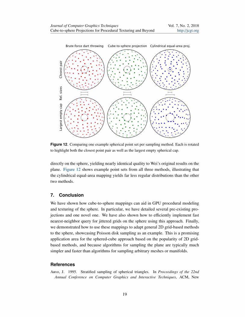
Figure 12. Comparing one example spherical point set per sampling method. Each is rotatedto highlight both the closest point pair as well as the largest empty spherical cap.

directly on the sphere, yielding nearly identical quality to Wei’s original results on theplane. Figure 12 shows example point sets from all three methods, illustrating thatthe cylindrical equal-area mapping yields far less regular distributions than the othertwo methods.

7. Conclusion

We have shown how cube-to-sphere mappings can aid in GPU procedural modelingand texturing of the sphere. In particular, we have detailed several pre-existing pro-jections and one novel one. We have also shown how to efficiently implement fastnearest-neighbor query for jittered grids on the sphere using this approach. Finally,we demonstrated how to use these mappings to adapt general 2D grid-based methodsto the sphere, showcasing Poisson disk sampling as an example. This is a promisingapplication area for the sphered-cube approach based on the popularity of 2D grid-based methods, and because algorithms for sampling the plane are typically muchsimpler and faster than algorithms for sampling arbitrary meshes or manifolds.

ReferencesArvo, J. 1995. Stratified sampling of spherical triangles. In Proceedings of the 22nd

Annual Conference on Computer Graphics and Interactive Techniques, ACM, New

19

Journal of Computer Graphics TechniquesCube-to-sphere Projections for Procedural Texturing and Beyond

Vol. 7, No. 2, 2018http://jcgt.org

York, ACM SIGGRAPH, 437–438. URL: https://dl.acm.org/citation.cfm?id=218380.218500. 2

Arvo, J. 2001. Stratified sampling of 2-manifolds. SIGGRAPH 2001Course Notes. URL: https://pdfs.semanticscholar.org/4b29/

674656bbf4067f23f0c24fe1b2e7ae198d7f.pdf. 2, 6, 8, 11

Bitterli, B., Novak, J., and Jarosz, W. 2015. Portalmasked environment map sampling.Computer Graphics Forum 34, 4, 13–19. URL: https://onlinelibrary.wiley.com/doi/abs/10.1111/cgf.12674. 9

Bowers, J., Wang, R., Wei, L.-Y., and Maletz, D. 2010. Parallel Poisson disk sampling withspectrum analysis on surfaces. ACM Transactions on Graphics (TOG) 29, 6, 166:1–166:10.URL: https://dl.acm.org/citation.cfm?id=1866188. 17

Brown, C., 2017. Bringing pixels front and center in VR video. URL:https://www.blog.google/products/google-vr/bringing-pixels-front-

and-center-vr-video/. 2, 6, 9, 16

Chan, F., and O’Neill, E. 1975. Feasibility study of a quadrilateralized spherical cube Earthdata base. Tech. Rep. 2-75, Environmental Prediction Research Facility, Naval Postgrad-uate School. URL: https://ntrl.ntis.gov/NTRL/dashboard/searchResults/titleDetail/ADA010232.xhtml. 2, 9, 11

Cline, D., Jeschke, S., White, K., Razdan, A., and Wonka, P. 2009. Dart throwing on surfaces.Computer Graphics Forum 28, 4, 1217–1226. URL: https://onlinelibrary.wiley.com/doi/full/10.1111/j.1467-8659.2009.01499.x. 17

Cook, R. L. 1986. Stochastic sampling in computer graphics. ACM Trans. Graph. 5, 1,51–72. URL: https://dl.acm.org/citation.cfm?id=8927. 17

Everitt, C., 2014. Twitter update. URL: https://twitter.com/casseveritt/status/550483976243412993. 10, 16

Everitt, C., 2016. “Projection” repository. URL: https://github.com/casseveritt/projection/blob/ee0c792a748d6786ce6010d839f4f1f43e71184b/envmap.h#

L197. 2, 10, 16

Gamito, M. N., and Maddock, S. C. 2009. Accurate multidimensional Poisson-disk sampling.ACM Transactions on Graphics (TOG) 29, 1, 8:1–8:19. URL: https://dl.acm.org/citation.cfm?id=1640451. 17

Gorski, K. M., Hivon, E., Banday, A., Wandelt, B. D., Hansen, F. K., Reinecke, M., and

Bartelmann, M. 2005. HEALPix: a framework for high-resolution discretization and fastanalysis of data distributed on the sphere. The Astrophysical Journal 622, 2, 759–771.URL: http://iopscience.iop.org/article/10.1086/427976/meta. 2

Greene, N. 1986. Environment mapping and other applications of world projections. IEEEComputer Graphics and Applications 6, 11, 21–29. URL: http://ieeexplore.ieee.org/abstract/document/4056759/. 2, 9

Heitz, E., Dupuy, J., Hill, S., and Neubelt, D. 2016. Real-time polygonal-light shading withlinearly transformed cosines. ACM Transactions on Graphics (TOG) 35, 4, 41:1–41:8.URL: https://dl.acm.org/citation.cfm?id=2925895. 2

20

Journal of Computer Graphics TechniquesCube-to-sphere Projections for Procedural Texturing and Beyond

Vol. 7, No. 2, 2018http://jcgt.org

Keinert, B., Innmann, M., Sanger, M., and Stamminger, M. 2015. Spherical Fibonaccimapping. ACM Transactions on Graphics (TOG) 34, 6, 193:1–193:7. URL: https://dl.acm.org/citation.cfm?id=2818131. 2, 4

Lagae, A., and Dutre, P. 2007. A comparison of methods for generating Poisson disk dis-tributions. Computer Graphics Forum 27, 1, 114–129. URL: https://onlinelibrary.wiley.com/doi/full/10.1111/j.1467-8659.2007.01100.x. 18

Lambers, M. 2016. Mappings between sphere, disc, and square. Journal of Computer Graph-ics Techniques Vol 5, 2, 1–21. URL: http://jcgt.org/published/0005/02/01/. 2

Marques, R., Bouville, C., Ribardiere, M., Santos, L. P., and Bouatouch, K. 2013. SphericalFibonacci point sets for illumination integrals. Computer Graphics Forum 32, 8, 134–143.URL: https://onlinelibrary.wiley.com/doi/pdf/10.1111/cgf.12190. 17

Meyer, Q., Smuth, J., Suner, G., Stamminger, M., and Greiner, G. 2010. On floating-point normal vectors. Computer Graphics Forum 29, 4, 1405–1409. URL: https://onlinelibrary.wiley.com/doi/full/10.1111/j.1467-8659.2010.01737.x. 2

Press, W. H., Teukolsky, S. A., Vetterling, W. T., and Flannery, B. P. 1992. Numericalrecipes in C. Cambridge University Press. URL: http://apps.nrbook.com/c/index.html. 13

Quılez, I., 2013. Shadertoy: Voronoi - 3D. URL: https://www.shadertoy.com/view/ldl3Dl. 4

Quılez, I., 2015. Voronoise. URL: http://www.iquilezles.org/www/articles/voronoise/voronoise.htm. 3

Shao, M.-Z., and Badler, N. 1996. Spherical sampling by Archimedes’ theorem. Tech.Rep. MS-CIS-96-02, University of Pennsylvania Department of Computer and InformationScience. URL: https://repository.upenn.edu/cgi/viewcontent.cgi?article=1188&context=cis_reports. 2

Singh, G. 2015. Sampling and variance analysis for Monte Carlo integration in sphericaldomain. PhD thesis, Universite Claude Bernard-Lyon I. URL: https://hal.archives-ouvertes.fr/tel-01217082/document. 2

Wei, L.-Y. 2008. Parallel Poisson disk sampling. ACM Transactions on Graphics (TOG) 27,3, 20:1–20:9. URL: https://dl.acm.org/citation.cfm?id=1360619. 17, 18

Wong, T.-T., Luk, W.-S., and Heng, P.-A. 1997. Sampling with Hammersley and Haltonpoints. Journal of Graphics Tools 2, 2, 9–24. URL: http://www.tandfonline.com/doi/abs/10.1080/10867651.1997.10487471. 2

Worley, S. 1996. A cellular texture basis function. In Proceedings of the 23rd annual confer-ence on computer graphics and interactive techniques, ACM, New York, SIGGRAPH ’96,ACM SIGGRAPH, 291–294. URL: https://dl.acm.org/citation.cfm?id=237267.3

21

Journal of Computer Graphics TechniquesCube-to-sphere Projections for Procedural Texturing and Beyond

Vol. 7, No. 2, 2018http://jcgt.org

Index of Supplemental MaterialsGLSL shader source code corresponding to many of the figures can be found online:

• Figures 1 and 4: Basic approach, jittered grid Voronoi diagramshttps://www.shadertoy.com/view/MtBGRD

• Figure 5, left: Space scenehttps://www.shadertoy.com/view/Mtj3DV

• Figure 5, right: Simulating brittle fracturehttps://www.shadertoy.com/view/llXXz4

• Figure 2: Value noise and Voronoisehttps://www.shadertoy.com/view/Ml2czm

• Figure 3: Comparison with Voronoi regions from 3D gridhttps://www.shadertoy.com/view/Xd3SRj

• Figure 6: All mappings, iterative inverse solvers, basis for benchmarkinghttps://www.shadertoy.com/view/XdlfDl

Thanks to Inigo Quılez and BeautyPi for maintaining Shadertoy.com and furnishing it withmany valuable examples.

Author Contact InformationMatt Zucker Yosuke HigashiSwarthmore College Swarthmore College500 College Avenue 500 College AvenueSwarthmore PA 19081, USA Swarthmore PA 19081, USAmzucker1@swarthmore.edu yhigash1@swarthmore.eduhttp://swarthmore.edu/NatSci/mzucker1

M. Zucker and Y. Higashi, Cube-to-sphere Projections for Procedural Texturing and Beyond,Journal of Computer Graphics Techniques (JCGT), vol. 7, no. 2, 1–22, 2018http://jcgt.org/published/0007/02/01/

Received: 2018-04-04Recommended: 2018-05-15 Corresponding Editor: Stephen HillPublished: 2018-06-26 Editor-in-Chief: Marc Olano

© 2018 M. Zucker and Y. Higashi (the Authors).The Authors provide this document (the Work) under the Creative Commons CC BY-ND3.0 license available online at http://creativecommons.org/licenses/by-nd/3.0/. The Authorsfurther grant permission for reuse of images and text from the first page of the Work, providedthat the reuse is for the purpose of promoting and/or summarizing the Work in scholarlyvenues and that any reuse is accompanied by a scientific citation to the Work.

22