curbside collection of recyclables. ii. simulation and economic analysis

Resources, Conservation and Recycling 22 (1998) 217–240

Curbside collection of recyclables. II. Simulationand economic analysis

Jess W. Everett a,*, Ramesh Dorairaj b, Sumit Maratha b,Patrick Riley c

a Ci6il and En6ironmental Engineering, Rowan Uni6ersity, Glassboro, NJ 08028, USAb School of Ci6il Engineering and En6ironmental Science, Uni6ersity of Oklahoma, Norman,

OK 73019, USA,c Waste Management of Oklahoma, Inc., 5600 N.W. 4th, Oklahoma City, OK 73127, USA

Accepted 20 March 1998

Abstract

Curbside collection of recyclable material can be expensive because the inherent costs ofcurbside collection are high, but also because amounts collected per residence are smallcompared to the total waste stream, and extra activity may be required, such as sorting. Inthis paper a simulation model is used to investigate the effect of collection method and routecharacteristics on route time. The simulation models presented calculate set-out amountbased on route characteristics, set-out rate (SOR), and participation rate (PR). Route timesare estimated for various conditions: constant SOR, constant PR, and constant set-outamount. Furthermore, a method for using route time to estimate vehicle and labor needs ispresented, and used to estimate economic costs for one and two-person crew collectionmethods for the three simulation conditions mentioned above. The two-person crew is foundto cost less than the one-person crew, for most simulated conditions. © 1998 Elsevier ScienceB.V. All rights reserved.

Keywords: Municipal solid waste; Recycling; Recyclables; Curbside collection; Economiccosts

* Corresponding author. Tel.: +1 405 3252282; fax: +1 405 3254217.

0921-3449/98/$19.00 © 1998 Elsevier Science B.V. All rights reserved.

PII S0921-3449(98)00014-7

J.W. E6erett et al. / Resources, Conser6ation and Recycling 22 (1998) 217–240218

1. Introduction

In the preceding paper [1], the authors presented an improved model capable ofestimating route time for recyclable curbside collection. The model calculated routetime as the sum of the times required to travel through a recyclables curbsidecollection route (travel time), collect set out material (collection time), and wait atstop signs and traffic lights (wait time). Collection time was estimated as a functionof the distance collectors walk to collect recyclables (walk time) and the mass ofmaterials sorted and loaded onto the collection vehicle (sort time).

The model estimates travel, walk, sort, and wait time using parameters derivedfrom observation of the collection method and the input of data describing thecollection route. Route descriptions include distances to all houses, vacant lots,intersections, stop signs, traffic lights, and break points. Break points indicate anobstruction to simultaneous set-out collection, such as a large vacant lot. The routedescription also indicates which houses have set-outs and the amount of materialset out at each house. The model was shown to be capable of estimating route timeto within 10% of observed values, on average, for two different collection methods.Errors greater than 15% were rare, and occurred on days when a crew member wasinjured (back injury) or when additional activities were required of the crew(placing promotional material in the bin). The two collection methods differed onlyin that one involved a single crew member (a driver/collector), while the otherutilized a two-person crew (driver/collector and passenger/collector).

By adding to the route time estimation model algorithms that, (1) estimateset-out amount based on route characteristics, including set-out rate and participa-tion rate, and (2) assign set-out status based on set-out rate, the model’s capabilitiescan be expanded to include collection simulation over a range of possible condi-tions, including ones that have not been observed in the field. The goal of this paperis to present just such a model, and to use the model to increase our understandingof the curbside collection of recyclables. Therefore, the objectives are to:� Present a route time simulation model for one and two-person crew collection

methods that can be used to simulate collection over a wide range of conditions,including variations in set-out rate, set-out amount, participation rate, andset-out distribution

� Present and discuss simulation results� Present a deterministic method for estimating vehicle and labor needs based on

route times calculated by the simulation model� Conduct an economic analysis of one and two-person collection methods using

the results of simulations� Present conclusions and recommendations for future research

2. Route time simulation model

Different recyclables collection routes can exhibit a wide range of set-out rates(SOR) and participation rates (PR). SOR is defined as the percent or fraction of

J.W. E6erett et al. / Resources, Conser6ation and Recycling 22 (1998) 217–240 219

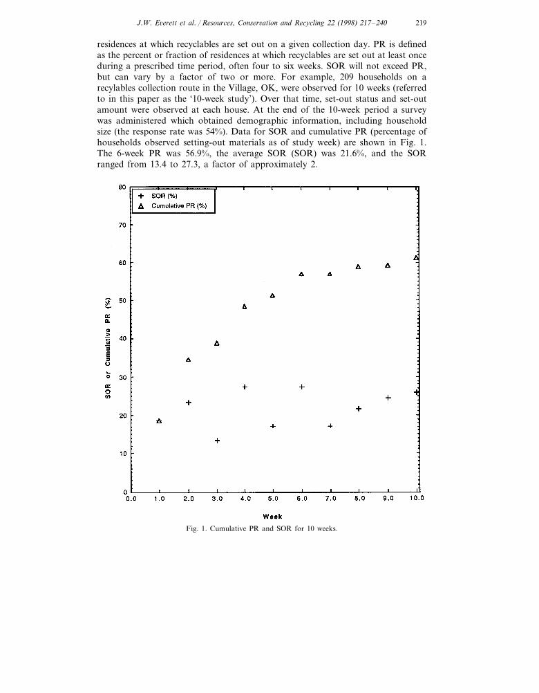
residences at which recyclables are set out on a given collection day. PR is definedas the percent or fraction of residences at which recyclables are set out at least onceduring a prescribed time period, often four to six weeks. SOR will not exceed PR,but can vary by a factor of two or more. For example, 209 households on arecylables collection route in the Village, OK, were observed for 10 weeks (referredto in this paper as the ‘10-week study’). Over that time, set-out status and set-outamount were observed at each house. At the end of the 10-week period a surveywas administered which obtained demographic information, including householdsize (the response rate was 54%). Data for SOR and cumulative PR (percentage ofhouseholds observed setting-out materials as of study week) are shown in Fig. 1.The 6-week PR was 56.9%, the average SOR (SOR) was 21.6%, and the SORranged from 13.4 to 27.3, a factor of approximately 2.

Fig. 1. Cumulative PR and SOR for 10 weeks.


Route time will vary with both SOR and PR; thus, route time estimation modelusers may wish to simulate various combinations of SOR and PR to determineroute time for a range of possible conditions. For example, someone studying theroute mentioned in the preceding paragraph might wish to simulate a 50–70% PRand a 10–30% SOR to determine if route time, and thus vehicle and labor needs,varies greatly. They may also wish to compare different collection methods overthis range of conditions; the route time simulation model can be used to do this.

SOR effects route time because it determines the number of collection stops,which effects walk time, sort time, and travel time. WaLk time and sort time areeffected because crew members must collect more set-outs. Travel time is effectedbecause there are more, shorter, travel events between stops, which result in aslower average travel speed. SOR and PR together effect the set out amount (SOA).SOA is defined as the amount of materials set out for collection by a setting outhousehold on a given collection day. Higher SOAs increase sort time.

It is necessary to differentiate between SOA at individual setting-out households(SOAi), the average set-out amount at setting-out households on a given route andcollection day (SOArc), and the average set-out amount on a route, over a numberof collection periods (SOArt). (SOArt) is a function of the average storage time fora route, which can be estimated as

STOR=CpPR

SOR(1)

where STOR is average storage time of participating households on a route, days;Cp is the time between collections, days; PR is participation rate, fraction ofpercent; and SOR is average set-out rate over a defined time period, fraction orpercent. For the 10-week study neighborhood, already mentioned, the collectionperiod was 1 week; thus, the average storage time was 18 days. This indicates thatthe average household stores recyclables for 2.6 weeks before setting them out forcollection. Because some of the households that set out materials during the 6-weekdetermination period may not have been regular recyclers, STOR is probablyoverstated to some unknown degree. For example, if a quarter of the 50 householdsthat only set out materials once during the first 6 weeks of observation were notregular participants, the PR would be approximately 51%, and STOR would be 17days.

The longer the storage time, all else equal, the larger SOArt, because householdsgather more materials before setting out. Therefore, according to Eq. (1), higherPRs and lower SORs will cause higher SOArts. A method for estimating SOArt

based on PR and SOR is given in the next subsection.When the route time simulation model is used to estimate route time for a range

of SORs and PRs, the model must take into account the fact that SOR and PR donot specify the distribution of set-outs throughout a route. Set-out distribution canhave a small effect on travel and walk time. Travel time is effected because differentset-out distributions result in different patterns of stops, which in turn effectsvehicle speed. Walk time is effected because distribution can effect the relativedistribution of one, two, and three set-out collections at single stops, thus effecting


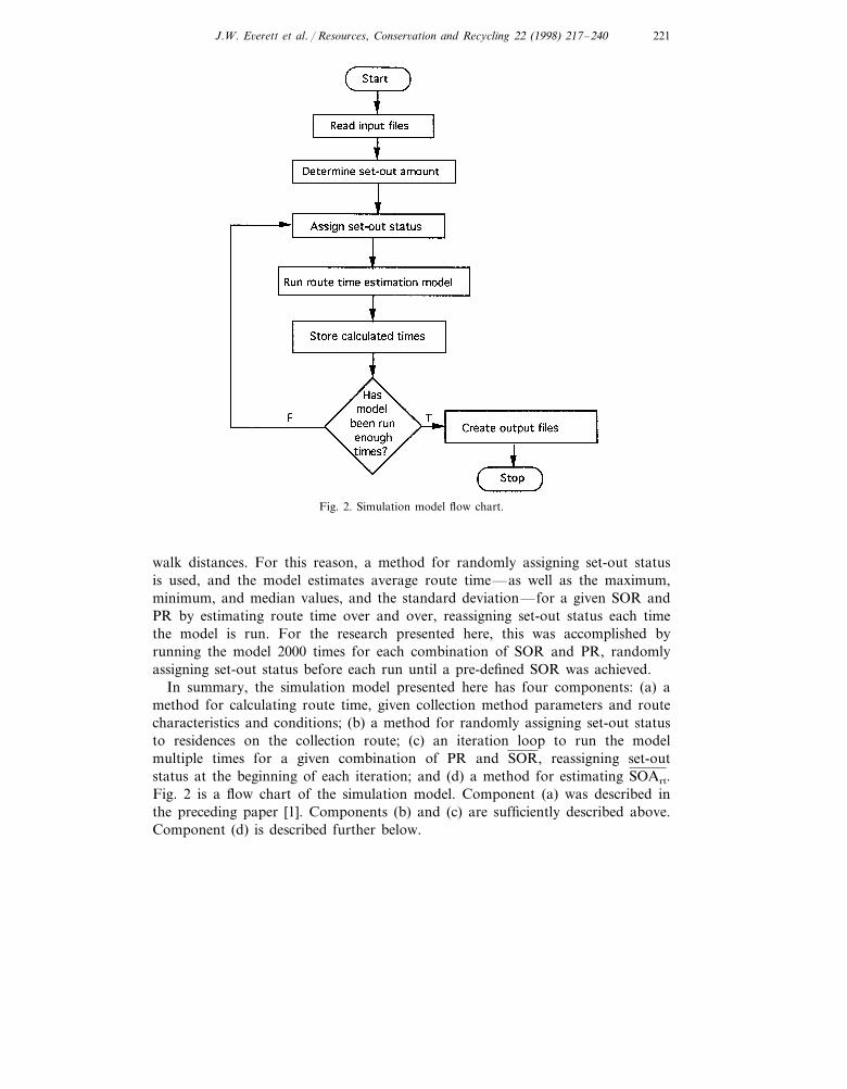
Fig. 2. Simulation model flow chart.

walk distances. For this reason, a method for randomly assigning set-out statusis used, and the model estimates average route time—as well as the maximum,minimum, and median values, and the standard deviation—for a given SOR andPR by estimating route time over and over, reassigning set-out status each timethe model is run. For the research presented here, this was accomplished byrunning the model 2000 times for each combination of SOR and PR, randomlyassigning set-out status before each run until a pre-defined SOR was achieved.

In summary, the simulation model presented here has four components: (a) amethod for calculating route time, given collection method parameters and routecharacteristics and conditions; (b) a method for randomly assigning set-out statusto residences on the collection route; (c) an iteration loop to run the modelmultiple times for a given combination of PR and SOR, reassigning set-outstatus at the beginning of each iteration; and (d) a method for estimating SOArt.Fig. 2 is a flow chart of the simulation model. Component (a) was described inthe preceding paper [1]. Components (b) and (c) are sufficiently described above.Component (d) is described further below.


3. Estimation of set-out amount (SOA)

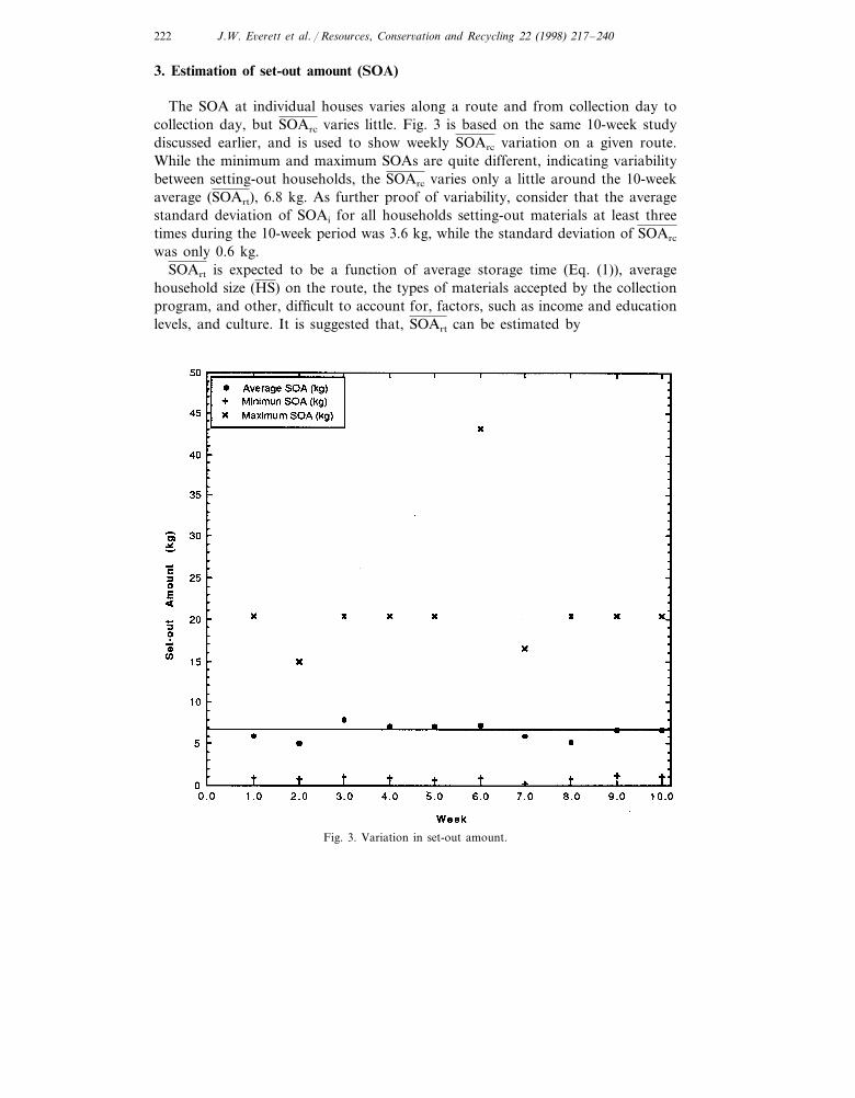
The SOA at individual houses varies along a route and from collection day tocollection day, but SOArc varies little. Fig. 3 is based on the same 10-week studydiscussed earlier, and is used to show weekly SOArc variation on a given route.While the minimum and maximum SOAs are quite different, indicating variabilitybetween setting-out households, the SOArc varies only a little around the 10-weekaverage (SOArt), 6.8 kg. As further proof of variability, consider that the averagestandard deviation of SOAi for all households setting-out materials at least threetimes during the 10-week period was 3.6 kg, while the standard deviation of SOArc

was only 0.6 kg.SOArt is expected to be a function of average storage time (Eq. (1)), average

household size (HS) on the route, the types of materials accepted by the collectionprogram, and other, difficult to account for, factors, such as income and educationlevels, and culture. It is suggested that, SOArt can be estimated by

Fig. 3. Variation in set-out amount.


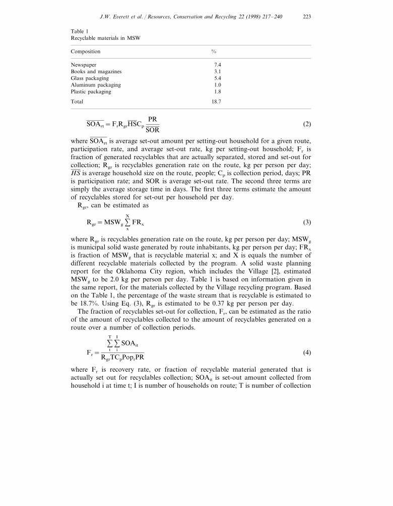
Table 1Recyclable materials in MSW

%Composition

Newspaper 7.43.1Books and magazines5.4Glass packaging1.0Aluminum packaging1.8Plastic packaging

18.7Total

SOArt=FrRgrHSCp

PR

SOR(2)

where SOArt is average set-out amount per setting-out household for a given route,participation rate, and average set-out rate, kg per setting-out household; Fr isfraction of generated recyclables that are actually separated, stored and set-out forcollection; Rgr is recyclables generation rate on the route, kg per person per day;HS is average household size on the route, people; Cp is collection period, days; PRis participation rate; and SOR is average set-out rate. The second three terms aresimply the average storage time in days. The first three terms estimate the amountof recyclables stored for set-out per household per day.

Rgr, can be estimated as

Rgr=MSWg %X

x

FRx (3)

where Rgr is recyclables generation rate on the route, kg per person per day; MSWg

is municipal solid waste generated by route inhabitants, kg per person per day; FRx

is fraction of MSWg that is recyclable material x; and X is equals the number ofdifferent recyclable materials collected by the program. A solid waste planningreport for the Oklahoma City region, which includes the Village [2], estimatedMSWg to be 2.0 kg per person per day. Table 1 is based on information given inthe same report, for the materials collected by the Village recycling program. Basedon the Table 1, the percentage of the waste stream that is recyclable is estimated tobe 18.7%. Using Eq. (3), Rgr is estimated to be 0.37 kg per person per day.

The fraction of recyclables set-out for collection, Fr, can be estimated as the ratioof the amount of recyclables collected to the amount of recyclables generated on aroute over a number of collection periods.

Fr=%T

t

%I

i

SOAit

RgrTCpPoprPR(4)

where Fr is recovery rate, or fraction of recyclable material generated that isactually set out for recyclables collection; SOAit is set-out amount collected fromhousehold i at time t; I is number of households on route; T is number of collection


days for which SOAit was measured; Cp is days in collection period; Popr is numberof people served by the program on the route; and PR is participation rate.

From the 10-week study and survey conducted in the Village, OK, the totalamount of recyclables collected from the 209 households over the 10 weeks wasdetermined to be 3033 kg. The average number of persons per household wasdetermined to be 2.2 for survey respondents. Using this as an estimate of averagehousehold size on the route indicates that Popr was 460. As already stated, the6-week PR was 56.9%. T was 10; Cp was 7 days. According to Eq. (3), Rg is 0.37kg per person per day. Using Eq. (4), Fr is estimated to be 0.45, indicating that forparticipants, 45% of generated recyclable materials are actually stored and set-outfor collection.

There are a number of reasons why Fr is not 100%. First, not all of the materialsthat fall within a general waste category are recyclable. For example, most recyclingprograms collect only PET and HDPE resins. Other plastic resins, then, are notrecyclable. In some cases, a recyclable product becomes un-recyclable during use.For example, a newspaper might be used to line an animal cage, or a jar used tohold a difficult to clean substance. Second, data obtained from the regional solidwaste report may not accurately describe the neighborhoods studied for thisresearch. Finally, and perhaps most importantly, people are not perfect recyclers;they fail to separate all of their recyclables from the general waste stream due toinattention, distractions, etc.

Entering the values for Fr, Rgr, HS, and Cp, Eq. (2) becomes

SOArt=2.6PR

SOR(5)

where SOArt is expressed as kg per setting-out house. Using the 56.9% PR and21.6% SOR, from the 10-week study, SOArt is estimated to be 6.8 kg, the same asactually measured (Fig. 3). Eq. (5) is incorporated in the simulation model. Eachtime the model assumes a new combination of PR and SOR, a corresponding SOArt

is calculated and used to estimate sort time. While the authors believe this equationto be applicable for the Village recycling program, other programs may havedifferent values of Fr, Rgr, HS, and Cp, and thus may require recalculation of Eq.(5).

4. Route time simulation results

Simulations were conducted to explore the effects of PR, SOA, and SOR. Ahypothetical route of 10000 houses with no traffic lights or stop signs was chosenfor the simulations. All adjacent residences were separated by the same distance,100 ft. Once per week collection was assumed. Parameters used to estimate travel,walk, sort, and wait time were derived from observation of the Village, OKrecycling program [1]. Set-out amount was estimated using Eq. (5) and set-outdistribution was assigned randomly for each model run to achieve the assignedSOR. The model was run 2000 times for each combination of SOR and PR, to


obtain minimum, maximum, and average values of route time, walk time, sort time,and collection time, as well as standard deviations.

There exists a triangular area of possible SOR and PR values. PR can vary from0 to 100%. SOR, however is bounded within a smaller range. First, for a given PR,SOR will not exceed PR. Furthermore, there is a limit to how small SOR can berelative to PR. As the ratio of PR to SOR increases, STOR increases according toEq. (1). For example, a PR of 100% and SOR of 1% for a program with once perweek collection (Cp=7 days) gives an average storage time of almost 2 years. It isunreasonable to assume that households, will or can store materials for this long.In this research it was assumed that the participants do not store recyclablematerials for more than 5 weeks on average, hence the ratio of PR to SOR islimited to 5 or less.

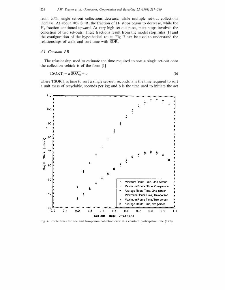
Rather than simulate the entire area of possible SOR and PR values, the authorshave chosen to simulate three conditions:� Constant participation rate (95%), SOR ranging from 20 to 95%� Constant set-out rate (20%), PR ranging from 20 to 95%� Constant set-out amount (6.8 kg), PR ranging from 5 to 100% (constant

PR/SOR ratio of approximately 2.7)Plots of maximum, minimum and mean route time for the one and two-person

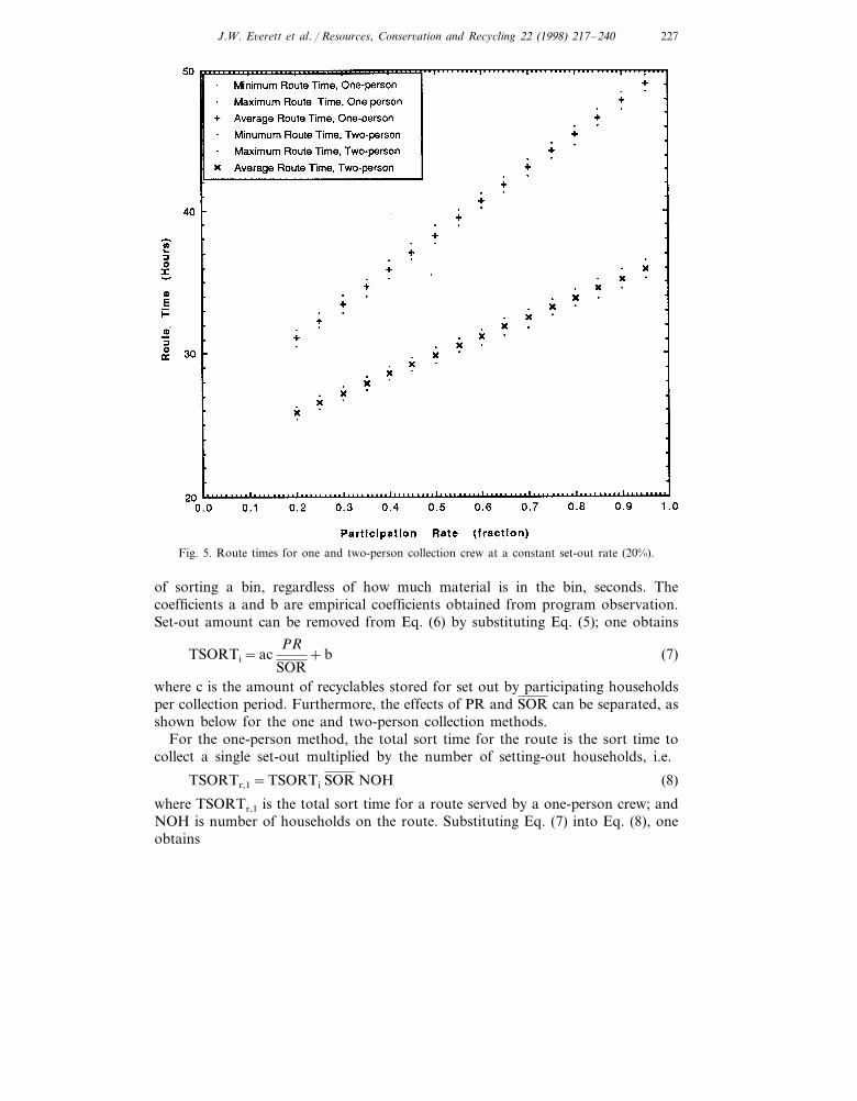
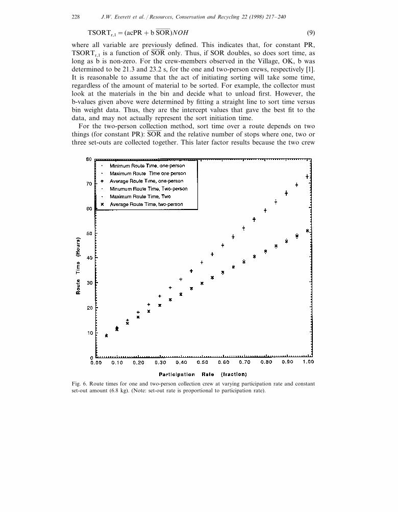
collection methods are shown in Figs. 4–6 for the three simulations. From theseplots, it can be seen that set-out distribution has little effect on route time, i.e. theminimum and maximum estimated route times lie close to the average values.Though not shown, this is also the case with walk, sort, and travel times. The threegraphs all show that route time is highest for the one person crew, as expected.Furthermore, the difference in route times for the one and two-person crewincreases with increasing SOR, PR, and SOArt. Finally, nearly linear increases inroute time are observed for the constant SOR and SOA figures. This is not so whenPR is held constant. In this case, route time reaches a peak at approximately 75%SOR but then declines at higher SORs.

Route time for the hypothetical route is the sum of travel, walk, and sort times.Though not shown here, graphs of walk and sort time indicate that both areimportant determinants of collection time, though sort time is generally mostimportant at higher SORs. For the collection methods and routes simulated here,collection time is larger than travel time, for all conditions except very low PR.Travel time is a nearly linear function of SOR. For the hypothetical route, it variesfrom approximately 8–15 h, as SOR varies from 20 to 95%. This is a minorcomponent of route time. Travel time varies little with PR or SOArt.

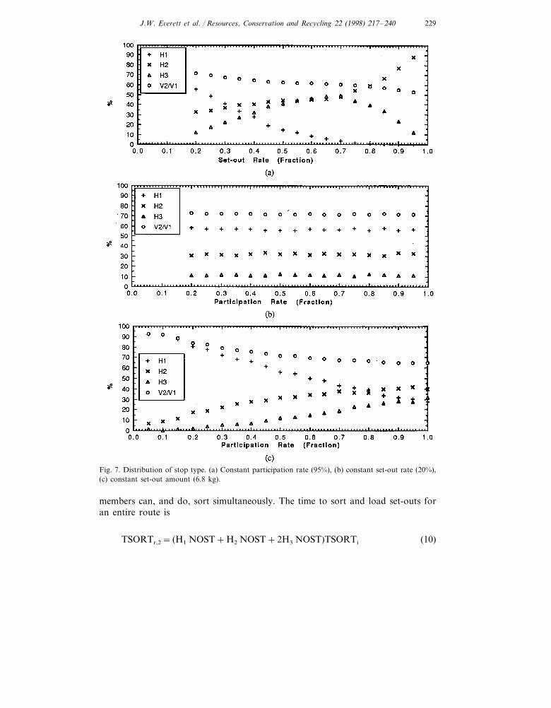
To understand walk and sort time variations it is necessary to examine thevariation in collection stop types that occurs as SOR is varied. Then, using theuniform nature of set-out amounts for the hypothetical neighborhood, a number ofequations can be derived. Let us define H1, H2, and H3 as the fraction of collectionstops along a route where one, two, or three set-outs are collected simultaneously,respectively, i.e. at single stops. Fig. 7(a–c) are used to show the percentage of stopsthat are H1, H2, and H3 for the same simulation conditions used to create Figs.4–6, respectively. From Fig. 7(a), it can be seen that, as the set-out rate increases


from 20%, single set-out collections decrease, while multiple set-out collectionsincrease. At about 70% SOR, the fraction of H3 stops began to decrease, while theH2 fraction continued upward. At very high set-out rates, most stops involved thecollection of two set-outs. These fractions result from the model stop rules [1] andthe configuration of the hypothetical route. Fig. 7 can be used to understand therelationships of walk and sort time with SOR.

4.1. Constant PR

The relationship used to estimate the time required to sort a single set-out ontothe collection vehicle is of the form [1]

TSORTi=a SOArt+b (6)

where TSORTi is time to sort a single set-out, seconds; a is the time required to sorta unit mass of recyclable, seconds per kg; and b is the time used to initiate the act

Fig. 4. Route times for one and two-person collection crew at a constant participation rate (95%).


Fig. 5. Route times for one and two-person collection crew at a constant set-out rate (20%).

of sorting a bin, regardless of how much material is in the bin, seconds. Thecoefficients a and b are empirical coefficients obtained from program observation.Set-out amount can be removed from Eq. (6) by substituting Eq. (5); one obtains

TSORTi=acPR

SOR+b (7)

where c is the amount of recyclables stored for set out by participating householdsper collection period. Furthermore, the effects of PR and SOR can be separated, asshown below for the one and two-person collection methods.

For the one-person method, the total sort time for the route is the sort time tocollect a single set-out multiplied by the number of setting-out households, i.e.

TSORTr,1=TSORTi SOR NOH (8)

where TSORTr,1 is the total sort time for a route served by a one-person crew; andNOH is number of households on the route. Substituting Eq. (7) into Eq. (8), oneobtains


TSORTr,1= (acPR+b SOR)NOH (9)

where all variable are previously defined. This indicates that, for constant PR,TSORTr,1 is a function of SOR only. Thus, if SOR doubles, so does sort time, aslong as b is non-zero. For the crew-members observed in the Village, OK, b wasdetermined to be 21.3 and 23.2 s, for the one and two-person crews, respectively [1].It is reasonable to assume that the act of initiating sorting will take some time,regardless of the amount of material to be sorted. For example, the collector mustlook at the materials in the bin and decide what to unload first. However, theb-values given above were determined by fitting a straight line to sort time versusbin weight data. Thus, they are the intercept values that gave the best fit to thedata, and may not actually represent the sort initiation time.

For the two-person collection method, sort time over a route depends on twothings (for constant PR): SOR and the relative number of stops where one, two orthree set-outs are collected together. This later factor results because the two crew

Fig. 6. Route times for one and two-person collection crew at varying participation rate and constantset-out amount (6.8 kg). (Note: set-out rate is proportional to participation rate).


Fig. 7. Distribution of stop type. (a) Constant participation rate (95%), (b) constant set-out rate (20%),(c) constant set-out amount (6.8 kg).

members can, and do, sort simultaneously. The time to sort and load set-outs foran entire route is

TSORTr,2= (H1 NOST+H2 NOST+2H3 NOST)TSORTi (10)


where TSORTr,2 is the total sort time for a route served by a two-person crew; andNOST is total number of collection stops. This equation is developed by consider-ing the elapsed sort time at a stop. If one set-out is collected (H1), then only oneTSORTi passes. If two set-outs are collected (H2), then, again, one TSORTi passes,because the two crew members collect simultaneously. Finally, if three set-outs arecollected, two TSORTis are used, because two set-outs are collected simultaneously,followed by separate collection of the third. It is easy to see that H2 and H3

collections are 2 and 1.5 times effective as H1 collections, respectively. From Eq.(10) it can be seen that H1+H2+2H3 is the number of individual set-out sort times(TSORTis) spent per stop.

Eq. (10) can be further modified to remove NOST. NOST can be written in termsof NOH, as

NOST=NOH SOR

H1+2H2+3H3

(11)

where all variables have been defined. Substituting Eqs. (7) and (11) into Eq. (10),one obtains

TSORTr,2= [acPR+b SOR]� H1+H2+2H3

H1+2H2+3H3

�NOH (12)

where all variables have been defined. For explanatory purposes, let v2 equalH1+H2+2H3 and v1 equal H1+2H2+3H3. Inspection of Eq. (12) indicates that,for constant PR, TSORTr,2 is directly proportional to b SOR v2/v1. Once again thecoefficient b is important, as it was for the one-person crew.

The main difference between the one and two-person collection methods lies inthe dependence of the two-person method on the ratio v2/v1. It can easily be shownthat, for the one person crew, v2/v1 is always equal to one. Inspection of Fig. 7(a–c)indicate that this is not so for the two-person crew. It has already been shown thatv2 is the fraction of TSORTi used per stop. From Eq. (11) it is clear thatH1+2H2+3H3 is the average number of setting-out households per stop. Thus,v2/v1 can be interpreted as the collection time per setting out household. The ratiov2/v1 is minimized by maximizing H2. Inspection of Fig. 7(a) indicates that as SORincreases, H2 increases, and thus v2/v1 declines. The effect of the two variables issuch that, though TSORTr,2 increases with SOR, it does so at a decreasing rate.Comparing the one and two-person collection methods, one can see that SOR v2/v1

varies from 0.2 to 0.95 for the one-person crew (v2/v1 is always 1 for the one-personcrew), but only 0.14 to 0.5 for the two-person crew, as SOR is varied from 0.2 to0.95. In summary, for constant PR, TSORTr,2 increases linearly with SOR for theone-person crew, but increases at a decreasing rate for the two.

Walk time relationships depend on SOR, stop type, and crew size. For theone-person crew, the single collector must walk to each and every set-out. At lowSOR, walk time is low, both because the number of set-outs is low and becausemost stops are type H1, allowing the truck to stop very close to the set-outs. AsSOR increases, walk time increases, both because more set outs must be walked toand because the number of diagonal H2 and H3 stops increases. Diagonal H2 stops


involve two setting-out houses located diagonally across the street, which requiredmore walking than across-the-street H2 stops. Finally, as the SOR becomes high,across-the-street H2 stops become dominant. Though the number of set-outs is stillincreasing, the opportunity to park the collection vehicle close to all of the set-outsresults in an actual decrease in walk time.

The phenomenon described above also applies to the two-person crew. Inaddition, ‘simultaneous walking’ provides even greater reduction in walk time athigh SOR, in a manner analogous to the savings already described for sort time.For the two-person crew, H2 stops have little crew ‘dead-time’, i.e. each crewmember simultaneously walks to a set-out. When one set-out is collected, one crewmember does no collection. When three set-outs are collected, two person crewmembers walk simultaneously to the first two set-outs, then one waits while theother collects the remaining bin. Because H2 stops dominate at high SOR, walktime decreases even more for the two-person crew (as compared to the one).

4.2. Constant set-out rate

Route times for constant SOR and PR ranging from 20 to 95%, for each crewsize, are presented in Fig. 5. Stop-type information is presented in Fig. 7(b).Because SOR remains constant, travel and walk times remain relatively constant foreach crew-size. Eqs. (9) and (12) can be used to estimate sort time. For theone-person crew, Eq. (9) indicates that sort time will increase proportionately toacPR. The increase with PR is a function of a, the time needed to sort a mass ofrecylables, and c, the amount of recyclables stored for set-out by participatinghousehold per collection period. Thus, ac is an estimate of the sort time required tocollect the amount of materials stored by a single setting-out household percollection period. Eq. (12) applies to the two-person crew. It indicates that sort timeis a function of acPR v2/v1. Because SOR is constant, v2/v1 is expected to vary little.As shown in Fig. 7(b), the ratio is approximately 0.72 over the PR range, indicatingthat the two-person crew uses 28% less sort time at SOR equal to 20%, as comparedto the one-person crew.

4.3. Constant set-out amount

For a constant set-out amount of 6.8 kg (a participation rate to set-out rate ratioof about 2.7), simulation results are given in Fig. 6. Route time increases on anearly linear manner for each collection method. At a very low participation rate(and low set-out rate) the two methods require almost identical route times. As theparticipation rate increases, the route time difference increases, with the one-personcrew taking longer. Stop-type information is presented in Fig. 7(c). Walk and traveltimes vary as already described for varying SOR. A constant PR to SOR ratio(called d) was used to maintain constant set-out amount. This allows the removalof SOR from Eqs. (9) and (12), resulting in the following equations. For theone-person crew, the equation is


TSORTr,1= (ac+bd)PR NOH (13)

while for the two-person crew the equation is

TSORTr,2= [ac+bd]PR� H1+H2+2H3

H1+2H2+3H3

�NOH (14)

where d is average number of collection periods between set-outs by participatinghouseholds. The combinations ac and bd are both sort time per participatinghousehold per collection period; ac can be considered to estimate the time toactually sort, while bd estimate the time to initiate a sorting event. Once again, thetwo crew-sizes differ in sort time by the ratio v2/v1. Inspection of Fig. 7(c) indicatesthat, for a set-out amount of 9.1 kg, the ratio varies from 0.92 to 0.65 as PR variesfrom 5 to 100%. Thus, the two-person crew has little advantage at low PR, but is35% more efficient at the maximum PR.

5. Estimation of vehicle and labor needs

One of the most important applications of the simulation method described inthis paper is the estimation of vehicle and labor needs, and, thus, costs. Adeterministic approach to estimating vehicle and labor needs [3,4], is presentedbelow. The method can be used to estimate the available time per route, therequired vehicle capacity, and the number of routes and vehicles required. Fromthis information, capital, operating, maintenance, and labor costs can be estimated.Given that the objective of an activity is to collect materials from residences, thetime available for each route is

Pscs=H(1−W)− (t1+ t2)

Nd

− (s+h) (15)

where Pscs is time spent collecting materials from residences on each route, from thefirst residence to the last, h/route; H is hours vehicle is on the road each workingday, h/working day; W is off-route time factor, consisting of the fraction of the dayspent in non-productive activities such as breaks; t1 is time spent at beginning ofday driving vehicle from dispatch area to first residence, h/working day; t2 is timespent at end of day driving vehicle from last residence to dispatch point, h/workingday; Nd is number of routes each vehicle can complete in a working day,routes/working day; s is time spent at the unloading site per route, h/route; and his round trip haul time from end of typical route to unloading site and back tobeginning of next route, h/route. A route consists of the path through a neighbor-hood taken while loading a collection vehicle. The maximum allowable number ofresidences per route is

Np=60

minhr

Pscsn

(tp)(16)


where Np is the number of residences/route, residences/route; n is the number ofcollectors riding on the vehicle, collectors; and tp is collector-time per residence (afunction of set-out rate and distribution, the number of collectors, the averagenumber of containers set out, the equipment used, the distances between pick-uppoints, the set-out point, e.g. curbside or backyard, etc.), collector-min/residence.The volume of material set out at each residence can be estimated as

VR=MPRCp

SW(17)

where VR is volume of waste collected at each residence during each collectionperiod, volume/residence; M is waste set out per person per day, mass/person/day;PR is persons per residence, persons/residence; Cp is the time between collections,days; and SW is density of waste as set out, mass/volume. Therefore, the requiredvolume of the collection vehicle is

Rv=VRNpSOR

r(18)

where Rv is required volume of vehicle, volume/route; SOR is setting-out rate as afraction; and r is compaction ratio. The number of routes that must be drivenduring each collection period is

Rcp=NOR

Np

(19)

where Rcp is the number of routes that must be driven each collection period,routes; and NOR is the number of residences that must be served each collectionperiod, residences.

Based on the parameters estimated using Eqs. (2)–(6), vehicle and labor require-ments can be estimated. The number of vehicles required is

NOV=Rcp

NdCWp

(20)

where NOV is the number of vehicles required to operate the collection program,unitless; and Cp is the number of working days in each collection period, workingdays. The labor requirements are

LR=n{RcpPscs+Ri

cp(s+h)+CWp (t1+ t2)}7

daysweek

(1−W)HCp

(21)

where LR is the labor requirements, collector-days/week; and Rcpi is the integer

number of routes in a collection period, i.e. the smallest integer larger than Rcp,routes.

A number of variables in Eqs. (15)–(21) are functions of collection practice (e.g.H, W, Cp, Nd, n, r, s) and the community and route layout (e.g. t1, t2, h).Reasonable values were assumed for the simulations presented here (Table 2). Onevariable, however, depends on route time. That variable is tp. It can be estimatedfrom route time as


tp=RTnNOH

(22)

where RT is route time for the hypothetical route, min.Labor and vehicle requirements were calculated using Eqs. (15)–(22), route times

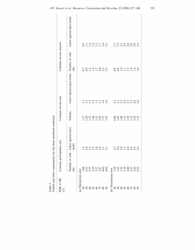
estimated by the simulation model, and the variable values given in Table 2. Theresults for all three simulations are presented in Table 3, for the one and two-personcollection methods. It can be seen that the labor requirements for the two-personcrew are higher than that for the one person method and the number of vehiclesrequired is higher for the one-person compared to the two-person collectionmethod.

6. Economic analysis

According to the program operator, labor costs were $10/h in 1996, while thecost of purchasing, maintaining, and operating the collection vehicle was $65/h [5].These cost factors were used in the analysis presented below. The vehicle and laborcosts, respectively, are calculated as

VCT=NOV CW

p H HVC

SOR NOH SOArt

(23)

and

LCT=LR H HLC

SOR NOH SOArt

(24)

where VCT is vehicle cost per ton of recyclable material collected, $/ton; HVC ishourly vehicle cost, $/h, LCT is labor cost per ton of recyclable material collected,$/ton; and HLC is hourly labor cost, $/h.

Table 2Variables used in vehicle and labor estimations

Parameter Value

H 8 h per working day0.15W

t1 0.3 ht2 0.3 h

0.2 hs0.25 hh2Nd

1 or 2nCp 7

10 000NORCp

W 5


Tab

le3

Veh

icle

and

labo

rre

quir

emen

tsfo

rth

eth

ree

sim

ulat

edco

ndit

ions

Con

stan

tse

t-ou

tam

ount

SOR

orP

RC

onst

ant

part

icip

atio

nra

teC

onst

ant

set-

out

rate

(%)

Num

ber

ofve

hi-

Lab

or(p

erso

n-da

ys/w

eek)

Lab

or(p

erso

n-da

ys/w

eek)

Veh

icle

sL

abor

(per

son-

days

/N

umbe

rof

vehi

-w

eek)

cles

cles

(a)

One

-per

son

crew

0.9

1.5

1.17

1.68

201.

20.

71.

30.

91.

130

2.33

2.0

1.26

1.2

1.3

1.2

401.

352.

772.

21.

43.

191.

42.

51.

441.

450

1.7

3.57

1.5

2.8

1.53

1.5

601.

71.

52.

01.

6370

3.0

3.87

1.6

2.2

1.9

3.1

801.

724.

052.

11.

812.

54.

023.

190

1.6

(b)

Tw

o-pe

rson

crew

2.2

0.6

1.7

2.7

200.

981.

381.

930

1.65

3.0

1.03

2.2

0.8

2.1

401.

02.

31.

921.

083.

41.

12.

182.

43.

71.

132.

450

2.5

1.3

2.6

602.

404.

01.

182.

81.

231.

470

2.5

2.57

4.2

1.6

2.63

3.0

4.3

1.28

2.6

802.

61.

83.

290

4.2

2.55

1.33


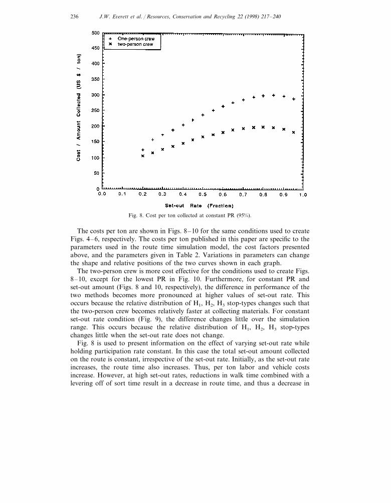
Fig. 8. Cost per ton collected at constant PR (95%).

The costs per ton are shown in Figs. 8–10 for the same conditions used to createFigs. 4–6, respectively. The costs per ton published in this paper are specific to theparameters used in the route time simulation model, the cost factors presentedabove, and the parameters given in Table 2. Variations in parameters can changethe shape and relative positions of the two curves shown in each graph.

The two-person crew is more cost effective for the conditions used to create Figs.8–10, except for the lowest PR in Fig. 10. Furthermore, for constant PR andset-out amount (Figs. 8 and 10, respectively), the difference in performance of thetwo methods becomes more pronounced at higher values of set-out rate. Thisoccurs because the relative distribution of H1, H2, H3 stop-types changes such thatthe two-person crew becomes relatively faster at collecting materials. For constantset-out rate condition (Fig. 9), the difference changes little over the simulationrange. This occurs because the relative distribution of H1, H2, H3 stop-typeschanges little when the set-out rate does not change.

Fig. 8 is used to present information on the effect of varying set-out rate whileholding participation rate constant. In this case the total set-out amount collectedon the route is constant, irrespective of the set-out rate. Initially, as the set-out rateincreases, the route time also increases. Thus, per ton labor and vehicle costsincrease. However, at high set-out rates, reductions in walk time combined with alevering off of sort time result in a decrease in route time, and thus a decrease in


per ton costs. For a given participation rate, and set-out rates below about 85%,cost minimization can be accomplished by minimizing set-out rate. This maximizesthe amount of materials collected per stop and minimizes the number of stops.Minimizing set-out rate relative to participation rate can happen only when storagetime increases; however, there is a limit to the amount of time a typical participantwill store recyclables.

Fig. 9 is used to present information on the effect of participation rate on costsper ton at a constant set-out rate. As the participation rate increases, the amountof material set-out by each residence increases and, hence, the total amount ofmaterial collected increases. Route time increases somewhat with participation rate,primarily because of sort time increases; however, the amount collected increases ata faster rate. Because of this, the total costs per ton decrease with increasingparticipation rate. This indicates that, at a given set-out rate, one should maximizeparticipation rate. At a set-out rate of 20%, increasing participation rate from 20 to90% decreases per ton costs by 70%.

Inspection of Figs. 8 and 9, indicates that program operators wishing to minimizecosts per ton should maximize participation (collect more material for a givenroute) and minimize set-out rate (minimize the number of stops). Program opera-tors have long know that increasing PR will maximize program efficiency. Theadvantages associated with minimizing SOR are less generally understood. The best

Fig. 9. Cost per ton at constant SOR (20%).


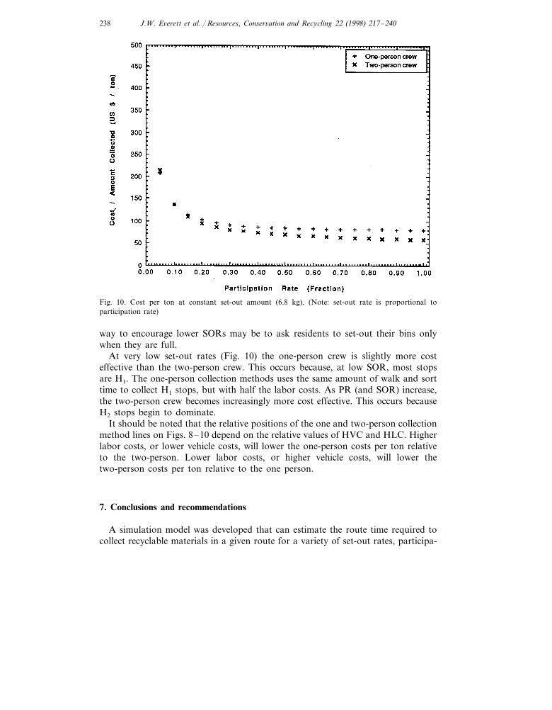
Fig. 10. Cost per ton at constant set-out amount (6.8 kg). (Note: set-out rate is proportional toparticipation rate)

way to encourage lower SORs may be to ask residents to set-out their bins onlywhen they are full.

At very low set-out rates (Fig. 10) the one-person crew is slightly more costeffective than the two-person crew. This occurs because, at low SOR, most stopsare H1. The one-person collection methods uses the same amount of walk and sorttime to collect H1 stops, but with half the labor costs. As PR (and SOR) increase,the two-person crew becomes increasingly more cost effective. This occurs becauseH2 stops begin to dominate.

It should be noted that the relative positions of the one and two-person collectionmethod lines on Figs. 8–10 depend on the relative values of HVC and HLC. Higherlabor costs, or lower vehicle costs, will lower the one-person costs per ton relativeto the two-person. Lower labor costs, or higher vehicle costs, will lower thetwo-person costs per ton relative to the one person.

7. Conclusions and recommendations

A simulation model was developed that can estimate the route time required tocollect recyclable materials in a given route for a variety of set-out rates, participa-


tion rates, set-out amounts, and set-out distributions. Collection method parame-ters and route characteristics serve as inputs to the model. A method for estimatingset-out amount as a function of set-out rate, participation rate, and participatinghousehold recyclables storage was developed for use in the simulation model.Set-out distribution is assigned randomly, according to an assigned set-out rate.The model is run multiple times for each set-out rate, allowing for the calculationof average, maximum, minimum, and standard deviations of route time. The modelis capable of estimating route times for both one and two-person collectionmethods, with commingled set-out and sorting at the collection vehicle.

Simulations were conducted at constant set-out rate, constant participation rate,and constant set-out amount. From these simulations, it was clear that set-outdistribution had little effect on route time. For each simulation, route time washighest for the one-person crew, as expected. Furthermore, the difference in routetimes for the one and two-person crew increased with increasing SOR, PR, andSOArt. Nearly linear increases in route time are observed for constant SOR andSOA. This was not so when PR was held constant. In this case, route time reacheda peak at approximately 75% SOR but then declined at higher SORs. Finally,collection time was larger than travel time, for all conditions except very low PR.

Some simulation results were explained by deriving a number of explicit equa-tions estimating sort time (Eqs. (9) and (12)–(14)). Explicit equations could bederived in this case, because of the uniform nature of the hypothetical neighbor-hood. These equations were used to understand the relationships between sort timeand set-out rate and participation rate for various simulation conditions. Somesimulation results were explained by examining the relative distribution of differenttypes of stops, i.e. H1, H2, and H3. It was determined that H2 stops are mosteffective (the least time required per set-out collected) in reducing walk time forboth the one and two-person crews and most effective for the two-person crew inreducing sort time (there is no effect for the one-person crew).

A method for using route time, estimated by the simulation model, to estimatevehicle and labor requirements was presented. As expected, the one-person crewhad higher vehicle requirements, but lower labor needs. Labor and vehicle costswere then used to estimate collection costs per ton of material collected. Thetwo-person crew was the most cost effective for the conditions simulated in thispaper, except at the lowest PR simulated (constant set-out amount). For constantPR and set-out amount, the difference in performance of the two methods becamemore pronounced at higher values of set-out rate. This occurred because the relativedistribution of H1, H2, H3 stop-types changed such that the two-person crewbecome relatively faster at collecting materials. For constant set-out rate condition,the difference appeared to stay relatively steady. This occurred because the relativedistribution of H1, H2, H3 stop-types changed little when the set out rate did notchange. Other labor and vehicle costs could change these conclusions drastically.Higher labor and lower vehicle costs would favor the one-person crew.

Future research should simulate collection for a number of different collectionmethods and routes. This will assist curbside collection recycling program operatorsin developing and implementing more efficient collection methods. Finally, the


model should be used to experiment with different stop rules, in an effort to identifymore efficient collection practice.

References

[1] Everett J, Maratha S, Dorairaj R, Riley P. Curbside collection of recyclables. I. Route timeestimation model. Resour Conserv Recycl 1998 (submitted).

[2] Benham Group, Inc. Metro Cities Solid Waste Management Plan. Phase 1 Study Report. Okla-homa City, OK: Benham Group, Inc., 1992.

[3] Tchobanoglous G, Thisen H, Vigil S. Integrated Solid Waste Management: Engineering Principlesand Management Issues. New York: McGraw Hill, 1993.

[4] Everett J, Shahi S. Curbside collection of yard waste. I. Estimating route time. J Environ EngASCE 1996;122(1):107–14.

[5] Armstrong B. Personal Communication. Oklahoma City, OK: BFI, 1996.

..

curbside collection of recyclables. ii. simulation and economic analysis

Documents