currency exchange rate forecasting di using machine ...docs.neu.edu.tr/library/6721800683.pdf ·...
TRANSCRIPT

WA
ZIR
MO
HA
MM
AD
I
CURRENCY EXCHANGE RATE FORECASTING
USING MACHINE LEARNING TECHNIQUES
A THESIS SUBMITTED TO THE GRADUATE
SCHOOL OF APPLIED SCIENCES
OF
NEAR EAST UNIVERSITY
By
WAZIR MOHAMMADI
In Partial Fulfillment of the Requirements for
the Degree of Master of Science
in
Information Systems Engineering
NICOSIA, 2019
CU
RR
EN
CY
EX
CH
AN
GE
RA
TE
FO
RE
CA
ST
ING
US
ING
MA
CH
INE
LE
AR
NIN
G T
EC
HN
IQU
ES
NE
U
2019

CURRENCY EXCHANGE RATE FORECASTING
USING MACHINE LEARNING TECHNIQUES
A THESIS SUBMITTED TO THE GRADUATE
SCHOOL OF APPLIED SCIENCES
OF
NEAR EAST UNIVERSITY
By
WAZIR MOHAMMADI
In Partial Fulfillment of the Requirements for
the Degree of Master of Science
in
Information Systems Engineering
NICOSIA, 2019

Wazir MOHAMMADI: CURRENCY EXCHANGE RATE FORECASTING USING
MACHINE LEARNING TECHNIQUES
Approval of Director of Graduate School of
Applied Sciences
Prof. Dr. Nadire ÇAVUŞ
We certify this thesis is satisfactory for the award of the degree of Masters of Science in
Information Systems Engineering
Examining Committee in Charge:
Assoc.Prof.Dr. Kamil Dimililer Department of Automotive Engineering, NEU
Assist.Prof.Dr. Yöney Kırsal EVER Department of Software Engineering, NEU
Assist.Prof.Dr. Boran ŞEKEROĞLU Department of Information Systems Engineering,
NEU (Supervisor)

I hereby declare that all information in this document has been obtained and presented in
accordance with academic rules and ethical conduct. I also declare that, as required by these rules
and conduct, I have fully cited and referenced all material and results that are not original to this
work.
Name, Last Name: Wazir Mohammadi
Signature:
Date:

To my family...

ii
ACKNOWLEDGMENTS
First and foremost, I give my thanks to an understanding supervisor Assist. Prof. Dr. Boran
ŞEKEROĞLU for his support, directions and for providing me guidance to start and complete
this research within the stipulated time.
Although, I must express my very profound gratitude to my parents and to my unaffected
family for providing me with unfailing support and continuous encouragement throughout my
years of study which is actually the whole of my life. This accomplishment would not have
been possible without them.
Thank you.
Wazir,
iii
ABSTRACT
The present Master’s thesis centers on forecasting currency exchange rates. The study seeks
the possibility of predicting future currency prices based on their historical data in FOREX
market. Four machine learning models; Backpropagation, Radial Basis Function (RBF), Long
Short-Term Memory, and Support Vector Regression (SVR) considered for conducting
forecasting tasks. The above models are developed and trained using python by deploying
three datasets from Swiss Duckascopy banking group. The currency pairs are EUR/USD,
USD/JPY and USD/TRY. The models trained, tested and compared to examine the strengths
and weaknesses of each of them. Furthermore, models have been verified with performance
evaluation techniques like Mean Squared Error (MSE), Root Mean Squared Error (RMSE) and
Mean Absolute Error (MAE) to identify the best model among those models. Experiments
shown that SVR outperformed other three techniques and Backpropagation performed least.
Keywords: currency exchange rate prediction; forex market; machine learning; artificial neural
networks; support vector regression
iv
ÖZET
Mevcut Yüksek Lisans tezi, döviz kurlarının tahmin edilmesine odaklanıyor. Çalışma
gelecekteki döviz fiyatlarını FOREX piyasasında tarihsel verilerine dayanarak tahmin etme
olasılığını araştırmaktadır. Dört makine öğrenim modeli; Geri yayılma, Radyal Temel İşlevi
(RBF), Uzun Kısa Süreli Bellek ve Öngörme görevlerinin yürütülmesi için düşünülen Destek
Vektör Regresyon (SVR) Kullanılmıştir. Yukarıdaki modeller İsviçre Duckascopy bankacılık
grubundan üç veri setini kullanarak python kullanarak geliştirilmiş ve eğitilmiştir. Döviz
çiftleri EUR / USD, USD / JPY ve USD / TRY'dir. Modeller, her birinin güçlü ve zayıf
yanlarını incelemek için eğitilmiş, test edilmiş ve karşılaştırılmıştır. Ayrıca, modeller, bu
modeller arasında en iyi modeli tanımlamak için Ortalama Kareler Hatası (MSE), Ortalama
Kareler Hatası (RMSE) gibi Kök ve Ortalama Mutlak Hata (MAE) gibi performans
değerlendirme teknikleriyle doğrulanmıştır. Deneyler, SVR'nin diğer üç teknikten daha iyi
performans gösterdiğini ve en azından geri yayılımın yapıldığını göstermektedir.
Anahtar Kelimeler: döviz kuru tahmini; forex pazarı; makine öğrenme; yapay sinir ağları;
destek vektör regresyon
v
TABLE OF CONTENTS
ACKNOWLEDGMENTS ........................................................................................................... iii
ABSTRACT .................................................................................................................................. iv
ÖZET .......................................................................................................................................... viii
LIST OF TABLES ........................................................................................................................ ix
LIST OF FIGURES ...................................................................................................................... ix
LIST OF ABBREVIATIONS .................................................................................................... xii
CHAPTER 1: INTRODUCTION
1.1 Background ............................................................................................................................ 1
1.2 The Problem ........................................................................................................................... 3
1.3 Aim of the Study .................................................................................................................... 4
1.4 Significance of the Study ....................................................................................................... 5
1.5 The Limitations of the Study ................................................................................................. 5
1.6 Overview of the Study ........................................................................................................... 6
CHAPTER 2: LITERATURE REVIEW
2.1 Forex Market & Currency Exchange Rate System ................................................................ 7
2.2 Factors Influencing FOREX Market ...................................................................................... 7
2.3 Machine Learning in Finance ................................................................................................ 9
2.4 Artificial Neural Networks .................................................................................................. 10
2.5 Support Vector Machine (SVM) .......................................................................................... 11
2.5.1 Support Vector Regression (SVR) .................................................................................... 12

vi
2.6 Related Studies..................................................................................................................... 13
2.6.1 Neural Networks Related Studies ................................................................................. 13
2.6.2 Fuzzy Related Studies .................................................................................................. 14
2.6.3 Support Vector Regression Related Studies ................................................................. 15
CHAPTER 3: MACHINE LEARNING TECHNIQUES
3.1 Machine Learning ................................................................................................................ 17
3.1.1 Supervised Learning ..................................................................................................... 18
3.1.2 Unsupervised Learning ................................................................................................. 19
3.1.3 Reinforcement Machine Learning ................................................................................ 20
3.2 Machine Learning Techniques ............................................................................................. 21
3.2.1 Artificial Neural Networks (ANNs) ............................................................................. 21
3.2.2 Support Vector Machine (SVR) ................................................................................... 29
CHAPTER 4: METHODOLOGY
4.1 Tools Used ........................................................................................................................... 32
4.1.1 Python .......................................................................................................................... 32
4.1.2 Jupyter Notebook ......................................................................................................... 35
4.1.3 Computer ..................................................................................................................... 35
4.1.4 Datasets ........................................................................................................................ 35
4.2 Data Preprocessing............................................................................................................... 38
4.3 Algorithms Overview........................................................................................................... 39
4.3.1 Training, Testing, and Validation ................................................................................ 39
4.3.2 Visualization ................................................................................................................ 39

vii
4.4 Model Development Summary ............................................................................................ 40
CHAPTER 5: RESULTS AND DISCUSSION
5.1 Experimental Setup .............................................................................................................. 41
5.2 Neural Network Algorithms ................................................................................................ 41
5.2.1 Backpropagation ........................................................................................................... 41
5.2.2 Radial Basis Function (RBF) ........................................................................................ 45
5.2.3 Long Short-Term Memory (LSTM) ............................................................................. 48
5.3 Support Vector Regression (SVR) ....................................................................................... 51
5.4 Comparison and the Best Model Among the Models .......................................................... 54
CHAPTER 6: CONCLUSION AND RECOMMENDATIONS
6.1 Future Works ....................................................................................................................... 55
REFERENCES ............................................................................................................................ 57

viii
LIST OF TABLES
Table 5. 1: Backpropagation training parameters ......................................................................... 42
Table 5. 2: EUR/USD training and testing evaluation results with Backpropagation .................. 42
Table 5. 3: USD/JPY training and testing evaluation results with Backpropagation ................... 43
Table 5. 4: USD/TRY training and testing evaluation results with Backpropagation .................. 43
Table 5. 5: RBF training parameters............................................................................................. 45
Table 5. 6: EUR/USD training and testing evaluation results with RBF ..................................... 45
Table 5. 7: USD/JPY training and testing evaluation results with RBF ....................................... 46
Table 5. 8: USD/TRY training and testing evaluation results with RBF ..................................... 46
Table 5. 9: LSTM training parameters ......................................................................................... 48
Table 5. 10: EUR/USD training and testing evaluation results with LSTM ................................ 48
Table 5. 11: USD/JPY training and testing evaluation results with LSTM.................................. 48
Table 5. 12: USD/TRY training and testing evaluation results with LSTM ................................ 49
Table 5. 13: SVR training parameters .......................................................................................... 51
Table 5. 14: EUR/USD training and testing evaluation results with SVR ................................... 52
Table 5. 15: USD/JPY training and testing evaluation results with SVR .................................... 52
Table 5. 16: USD/TRY training and testing evaluation results with SVR ................................... 52

ix
LIST OF FIGURES
Figure 2. 1: Currency price influencing factors (compareremit.com, 2018) .................................. 8
Figure 2. 2: Neural Network (Kalghatgi et al., 2015) .................................................................. 11
Figure 2. 3: SVM application (Diggdata.in, 2018) ....................................................................... 12
Figure 2. 4: Models process flow ................................................................................................. 16
Figure 3. 1: Supervised Learning model diagram ........................................................................ 19
Figure 3. 2: Unsupervised learning model diagram ..................................................................... 20
Figure 3. 3: Reinforcement learning diagram (UCBWiki, 2016) ................................................. 21
Figure 3. 4: ANN elements diagram (Bre, Gimenez, & Fachinotti, 2018) .................................. 23
Figure 3. 5: Artificial Neuron illustration (Abraham, 2005) ........................................................ 24
Figure 3. 6: LSTM architecture with single cell block ................................................................. 25
Figure 3. 7: RBF structure ............................................................................................................ 26
Figure 3. 8: Normalized and Un-Normalized RBF (Shorten & Murray-Smith, 1994) ................ 27
Figure 3. 9: Backpropagation Learning process ........................................................................... 29
Figure 3. 10: Linear SVR (Sayad, 2017) ...................................................................................... 30
Figure 3. 11: Nonlinear SVR (Sayad, 2017) ................................................................................ 31
Figure 4. 1: A Tensorflow Dataflow Diagram (Abadi et al., 2016) ............................................. 34
Figure 4. 2: EUR/USD rate of the dataset .................................................................................... 36
Figure 4. 3: USD/JPY rate of the dataset ..................................................................................... 37
Figure 4. 4: USD/TRY rate of the dataset .................................................................................... 37
Figure 4. 5: Entire process flow diagram ..................................................................................... 40
Figure 5. 1: EUR/USD actual and predicted price visualization with Backpropagation ............. 44
Figure 5. 2: USD/JPY actual and predicted price visualization with Backpropagation ............... 44
Figure 5. 3: USD/TRY actual and predicted price visualization with Backpropagation ............. 44
Figure 5. 4: EUR/USD actual and predicted price visualization with RBF ................................. 47
Figure 5. 5: USD/JPY actual and predicted price visualization with RBF .................................. 47
Figure 5. 6: USD/TRY actual and predicted price visualization with RBF ................................. 47
Figure 5. 7: EUR/USD actual and predicted price visualization with LSTM .............................. 50
Figure 5. 8: USD/JPY actual and predicted price visualization with LSTM ............................... 50
x
Figure 5. 9: USD/TRY actual and predicted price visualization with LSTM .............................. 50
Figure 5. 10: EUR/USD actual and predicted price visualization with SVR ............................... 53
Figure 5. 11: USD/JPY actual and predicted price visualization with SVR ................................ 53
Figure 5. 12: USD/TRY actual and predicted price visualization with SVR ............................... 53
Figure 5. 13: Error Comparison of 4 models ................................................................................ 54
xi
LIST OF ABBREVIATIONS
ANN Artificial Neural Network
FOREX Foreign Exchange Market
CNN Convolutional Neural Networks
KNN K Nearest Neighbors
LR Linear Regression
ML Machine Learning
MLP Multi-Layer Perceptron
RELU Rectified Linear Unit
RMSE
MSE
Root Mean Squared Error
Mean Squared Error
MAE Mean Absolute Error
AI Artificial Intelligence
OTC Over The Counter
RNN Recurrent Neural Network
LSTM Long Short-Term Memory
RBF Radial Basis Function
SVR Support Vector Regression
SVM Support Vector Machine
OCR Optical Character Recognition
FTS Fuzzy Time Series
SRM Structural Risk Minimization
ERM Empirical Risk Minimization
1
CHAPTER 1
INTRODUCTION
1.1 Background
In the early societies, the exchange of goods was usually carried out in a swap. In such a
system, a certain amount of a good was exchanged for a certain amount of other goods. This
system can only be used in small communities, and as human societies grow larger, goods
need to be exchanged by money. In the old days, money was usually one of the goods in those
communities. For example, in the Middle East, barley was used as money or pearl were used
as money in America's Continent. According to Herodotus (440 BC), the people of Lydia were
the first to use the silver coin. With the expansion of banks, bank receipts expanded as money.
Between the 17th and 19th centuries, most European countries used the gold standard, in
which paper money had a fixed and stable value to gold.
After the Second World War at the Bretton Woods Conference, most countries in the world
turned to Fiat's currency, which was proven in US dollars, and the US dollar was the only
currency with stable value against gold. In 1971, at the time of Richard Nixon (United States
president 1969-1974), the United States abolished the Bretton Woods treaty unilaterally, and
since then, all the money used in the world has become Fiat money. Afterward and especially
after electronic revolution trading grows between countries and different people with different
currencies. As we all know currency is a monetary system in general use of a particular
country. Because of the intrinsic or absolute value that the currency holds, people started
buying or selling currency itself for exchanging of another currency. These concepts gradually
built Foreign Exchange Market (FOREX, FX or Currency Market).
FOREX market is one of the largest and extremely liquid (an asset that can be exchanged for
money, i.e. currencies, shares, bonds etc.) markets for traders and investors (Diego, Ildar &
Oleksiy, 2017). According to the Bank of International Settlement (2016), the average trading
in Forex market was 5.1$ trillion dollars per day in April 2016. For this purpose, usually, a
pair of currency exchanged, the currency that an investor can sell or buy is called base

2
currency. The one that an investor wants to pay or receive for the base currency is called
reference currency. It is a decentralized market, which although refers to Over the Counter
(OTC) market. In OTC market, trading is done directly between two parties with no control of
any government. It does not have a physical location as well. The transactions made by
computer, phone and email orders (Diego et al., 2017).
For being able to make transactions in Forex market the trader must have an account with a
brokerage company. As the OTC is digitized and works on networks, investors are able to
create accounts from another country but the best suggestion would be to choose a trusty
broker. For instance, a broker with the biggest capital liquidity. The main trading centers are
London and New York City, though Tokyo, Hong Kong, and Singapore are all important
centers as well. Additionally, Banks throughout the world participate.
Considering the above issues; governments, banks, investors, and traders would not like to buy
or sell currencies randomly. They would consider analysis and forecasting for their target
currencies both in short and long time movements. They have their eyes on different factors
which affect market changes. They are trying to “buy low” and “sell high” whenever the price
is rise. An investor buys the currency which he/she thinks will rise in a time interval. Since the
market is digitized the prices going up or down in seconds, a specific political action or change
to any other affective factor can change the market rapidly.
Furthermore, it is often argued that predicting currency exchange rate is a futile struggle
(Tomas, 2007). According to (Goodman, 1978; Frankel & Rose, 1995) Forex market is
considered to be an efficient market. Already Mussa (1979) believes that the nature of Forex is
unpredictable, it is a random walk and major dollar exchange rates follow this concept. The
market is efficient, it means everybody has access to all available information so everybody is
able to build strong efficient hypothesis. The historical data of exchange rate does not hold any
information which can help participants or investors to accurately predict the future exchange
rate. Evidence shows every second a news could change the direction of the rates. But that is
not just the case, companies, investors, banks and almost all participants are recruiting
professionals, forecasters and experts and definitely they would use their forecasting in their
decisions. By the way, historical data can predict gradually increase or decrease unless there is

3
a big change in the market. The market movement is based on professional’s decisions though
making a prediction is always a good help for Forex participants, it also depends on how
accurate the prediction models are. Actually, Changes are rapidly happening in the market but
most of them are repetitive which it happened many times before, put that in mind it makes
sense to predict same changes, though historical data holds these kinds of information. Mark
(1995) believes that the models were useful for currency exchange rate prediction at long
horizons. Time passed and nowadays we are living in the era of Artificial intelligence (AI),
robotics and machine learning. A lot of machine learning models have been tested for Forex
forecasting which most of them gave a good result and accuracy rate.
Researchers tried to forecast Forex both in classification and regression way, by classification
they defined whether the price of our target currency going to be rise or fall down which is
actually called binary classification. Another way is regression which they tried to predict the
exact value of the currency in a period of time in the future.
This study aims to predict forex in a regression way, which is predicting the target currency
value in the future. Four prediction models are going to be tested in a comparison manner and
the best one will be chosen among them at the end. The models are Recurrent Neural Network
(LSTM), Backpropagation, Radial Basis Function (RBF), and Support Vector Regression
(SVR). Five attributes and features are going to be used from the datasets (Open, Close, High,
Low and Volume).
1.2 The Problem
Forex market is big and grow larger by the concept of globalization. As mentioned above,
According to the Bank of International Settlement (2016) the average trading in Forex market
was 5.1$ trillion dollars per day in April 2016. Furthermore, countries are connected all over
the world through air, land, and seas. Economic grows every day, import and exports are
increased excessively. People have to exchange their currencies with different currencies of
their needs. Saying all these proves one thing the importance of the currency price changes.
Putting this in mind, being aware of these changes made possible by appropriate Forecasting
techniques. Considering the digitization of the forex market, prices are changing fast, it may
4
harm investors, banks, and all participants even though countries economy are highly
dependent on their currency value in global market. Taking cognitive decisions by an investor,
decrease the volume of risk and prevent big losses.
Forex market produces a lot of data daily which is connected to the market movements. At the
same time, it holds the causes which rise or falling down the price of the currencies. These
data are available and accessible for everybody. In the other hand, machine learning
algorithms improved impressively. They are being used in fraud detection, weather prediction,
stock prediction, sickness prediction, pollution prediction etc. so considering of what’s
mentioned, putting all these together to forecast the currency exchange rate is crucial to all
participants of forex and that’s what this study is intended to do. Investors should be reminded
and notified about the change possibilities in the future of the market.
1.3 Aim of the Study
To declare techniques that yield highest accuracy and minimum error to forecast three pairs of
currency in forex market. These three pairs are namely: EUR/USD, USD/TRY, and USD/JPY.
Different supervised ML models developed using python programming language with the help
of its libraries like tensorflow, keras, matplotlib etc.
The models are tested on in order (13, 11, and 13) years of forex historical data on mentioned
currencies. The data is downloaded from Duckascopy Swiss banking group. The reason why
Turkish lira is 11 years is that they don’t have the records before 2007.
Time series data is good to be predicted using ML algorithms. A lot of researches have been
done on this topic with different algorithms. The purpose of this research is to compare 4 of
the suggested models. They are being tested with the mentioned three pairs of currency. The
result is compared to determine the model with minimum loss function and less errors. The
models being tested in this study are as follows:
Long Short-Term Memory (LSTM)
Backpropagation
Radial Basis Function (RBF)

5
Support Vector Regression (SVR)
1.4 Significance of the Study
Forex market transactions give a clear picture of how big and important the currency market
is. A lot of money being exchanged daily, it affects countries and global economy obviously.
Currency exchange forecasting will make investors aware of what is going to happen in the
market. It helps them take reliable decisions and decrease risk intensity. If the technology has
proven to work accurately it will spread widely, that will make the market a bit stable as long
as the profit may decrease as well. Considering what is mentioned above research in this field
is worthy and demanded.
Machine learning in computer information systems is widely used in financial industries.
Experts rely on what the automated systems and algorithms suggest them. It helps
organizations for decision making-processes based on its predictive abilities. Almost all of the
big financial companies and banks started using Machine learning and Artificial Intelligence
in their organizations which shows the significance of the researches in this area. For instance,
three pairs of currencies used in this study EUR/USD, USD/JPY and USD/TRY play a crucial
role in forex market. Analyzing their future movements would help involved companies,
investors and generally traders.
Researches excessively conducted on this field. This study is using three pairs of currencies
which each of them had its own rise and fall with four supervised ML models in a comparative
way. Furthermore, different optimization, regularization, and validation techniques have been
used to achieve bests of the models. On the other hand, the best model among them will be
presented at the end which is more accurate with less errors. Finally, the data being used in
this research is from 11 to 13 years which yields rise and downs in prices that gives models the
ability to forecast well.
1.5 The Limitations of the Study
Despite the fact that this research reached to its goals, it would have been more accurate and
correct if some sentiment analysis of the news and financial news have been done on the

6
market and the result combined as a feature with our data in the dataset. In addition, there are
factors which influence prices in the market like inflation, government’s depth, political
stability of the countries etc. including these factors and combining them all together helps the
result to be precise and more reliable.
1.6 Overview of the Study
The research made up of six chapters in all:
Chapter 1: gives an insight of the financial terms including Forex, currency, and others,
although the way it works in the market. It also describes the machine learning techniques
used for Forecasting. After that aim of the research, its importance, limitations and research
outline is described.
Chapter 2: a briefing of the past related researches will be given with their techniques and
results.
Chapter 3: explain the theory and application of the machine learning techniques and their
philosophy.
Chapter 4: algorithms and models being used in this thesis will be explained in details with
their backend mathematical formulas.
Chapter 5: discuss the outcome and result of the study.
Chapter 6: Finalize the thesis, conclude the result and importance and provide
recommendations for future improvements.

7
CHAPTER 2
LITERATURE REVIEW
In this chapter, the following topics are discussed; first of all, a brief explanation of forex
market with currency exchange system along factors influence this market and causes
currencies to rise and fall in their prices presented. Although machine learning in financial
topics especially predicting future possible events and accidents described. A brief review of
the regression forecasting and related problems provided. Meanwhile, background of the
algorithms used in this research is presented. Finally, previously related researches and studies
published were examined and reviewed.
2.1 Forex Market & Currency Exchange Rate System
The foreign exchange market is fundamentally classified as a liquid market where the
information is public and accessible for all traders equally (Andrew & Victor, 2003). They
share the same expectations which make the forex exchange rate more dependent. At the same
time central banks of each country and many more agencies around the world working closely
to stable or increase the value of their currencies (Znaczko, 2013). For instance, the Federal
Reserve Bank of New York is responsible for foreign exchange rate related activities in U.S.
The bank monitors and analyzes the global financial market changes, it manages the U.S.
foreign currency reserve and intervenes in the market whenever demanded from time to time.
The bank buys dollar and sells foreign currencies to support the value of the dollar or sells
dollar and buys foreign currencies to apply descending weight on the cost of the dollar (FRB,
2004).
2.2 Factors Influencing FOREX Market
Before jumping to forecasting and prediction of the forex and currency exchange rates all
factors influenced the currency prices to appreciate or depreciate need to be analyzed because
the prices depend on many factors. Future events of these factors will change the prices in the
market as well. So basically understanding the factors are crucial in order to understand the

8
market pulse. According to (Patel, et al. 2014) eleven factors influencing currency prices are
as follows:
1. Inflation
2. Rate of interest
3. Capital account balance
4. Role of speculators
5. Cost of manufacture
6. Debt of the country
7. Gross domestic product
8. Political stability and economic performance
9. Employment data
10. Relative strength of other currencies
11. Macroeconomic and geopolitical events
Figure 2.1: Currency price influencing factors (compareremit.com, 2018)
Each and every single one of these factors has its own effects on currency valuation,
appreciation and depreciation of currencies are highly dependent on these factors. For
instance, let’s see how rates of interest affects currency prices in the markets. If the rate of
interest of a country increases it means that country being attracted by investors, when
investors invest on that country they will receive more returns from their savings which is

9
mostly on the country’s currency. So the demand for that currency increases and it affects the
appreciation of the inflow of the currency which results a higher price in the market as well.
Though financial companies recruit professionals and experts to use available tools and predict
possible directions of different currencies base on these factors. One of these tools is Machine
Learning which the usage is growing by the time passing.
2.3 Machine Learning in Finance
ML techniques have shown an impressive performance in solving many real-life problems. It
has been used in different fields. We can divide researches in this are in two categories,
classification, and regression.
Classification: a classification problem is when the output is a label or category for example
“blue”, “red” and “black” or “positive” and “negative”. Usually, inputs are given to the
classification models and attempt to generalize and predict one or more outputs.
Regression: a regression problem is when the output variable is a real or continuous value like
“salary”, “currency exchange price” or “weight”. The models are trying to predict these values
as accurate as possible.
The following is a briefing of the previous studies on this two categories:
It’s being used in classification problems like: communications (Di, 2007), internet traffic
analysis (Nguyen & Armitage, 2008), medical imaging (Wernick, Yang, Brankov,
Yourganov, & Strother, 2010), astronomy (Freed & Lee, 2013), biology (Zamani &
Kremer, 2011) and time series analysis (Qi & Zhang, 2008). They also study evaluating
sentiments in financial news and conducting text analysis of the market and world
financial news few examples are predictive machine learning technique for financial news
articles (Schumaker, 2009), document analysis (Khan, Baharudin, Khan, & E-Malik,
2009).
For regression problems algorithms like linear regression, SVR, Decision trees, random
forest, and different ANNs are used. ANNs are the most used algorithms in regression
problems especially when deep learning used in forecasting and predictions. Some of these
studies are Forex trading system (Pujari Et al., 2018), Forex prediction using CGP and

10
RNN (Rehman et al., 2014) and Conditional time series forecasting with convolutional
neural networks (Borovykh et al., 2017)
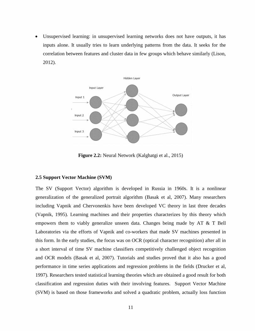
2.4 Artificial Neural Networks
Neural networks are designed in a parallel interconnected network. They have simple elements
and their hierarchal organizations in their structure, which are designed to communicate with
real world objects in a biological nervous systems way (Zhang and Zhou, 2006). The first
studies about neural network has done in 1943 by McCulloch and Pitts which they developed
M-P neuron model. After that significant studies conducted in 1950s and 1960s on single layer
neural networks. Single layer neural networks are good for classifying some patterns but they
have many limitations and restrictions in their learning capabilities. For instance, they cannot
easily learn a simple function like XOR.
This limitation avoided researches on the years 1970s because of the weak learning
capabilities but back in the early of 1980s studies on neural network extensively resurged
insomuch of multilayer neural network creation and high capable successful learning
algorithms. Nowadays different kind of algorithms exist and it’s being used widely in all fields
and sectors. From medical application to financial systems to face recognition and voice
recognition systems and so forth. A good practice about neural networks is that they use
practical techniques for learning from the examples which this concept have been used in
various areas. Currently, many neural networks being used by experts such as self-organizing
feature mapping networks, radial basis function networks, adaptive resonance theory models
and multi-layer feed forward neural networks (Kalghatgi et al., 2015).
There are two learning strategies in machine learning where neural networks used both of
them and can easily fit for both of them. These strategies called supervise learning and
unsupervised learning.
Supervised learning: in supervised learning the network training data has encoded in pairs
which include inputs and outputs. The outputs are usually noted. Network tries to
understand the relationship between input and output. It tries different weights to adjust
and produce the same result as the correct output with various scenarios (Lison, 2012).
11
Unsupervised learning: in unsupervised learning networks does not have outputs, it has
inputs alone. It usually tries to learn underlying patterns from the data. It seeks for the
correlation between features and cluster data in few groups which behave similarly (Lison,
2012).
Figure 2.2: Neural Network (Kalghatgi et al., 2015)
2.5 Support Vector Machine (SVM)
The SV (Support Vector) algorithm is developed in Russia in 1960s. It is a nonlinear
generalization of the generalized portrait algorithm (Basak et al, 2007). Many researchers
including Vapnik and Chervonenkis have been developed VC theory in last three decades
(Vapnik, 1995). Learning machines and their properties characterizes by this theory which
empowers them to viably generalize unseen data. Changes being made by AT & T Bell
Laboratories via the efforts of Vapnik and co-workers that made SV machines presented in
this form. In the early studies, the focus was on OCR (optical character recognition) after all in
a short interval of time SV machine classifiers competitively challenged object recognition
and OCR models (Basak et al, 2007). Tutorials and studies proved that it also has a good
performance in time series applications and regression problems in the fields (Drucker et al,
1997). Researchers tested statistical learning theories which are obtained a good result for both
classification and regression duties with their involving features. Support Vector Machine
(SVM) is based on those frameworks and solved a quadratic problem, actually loss function
12
and regularization term combined to give the convex objective function to minimize errors.
SVR attempts to minimize the generalize error bound instead of observed training error to
achieve a better performance.
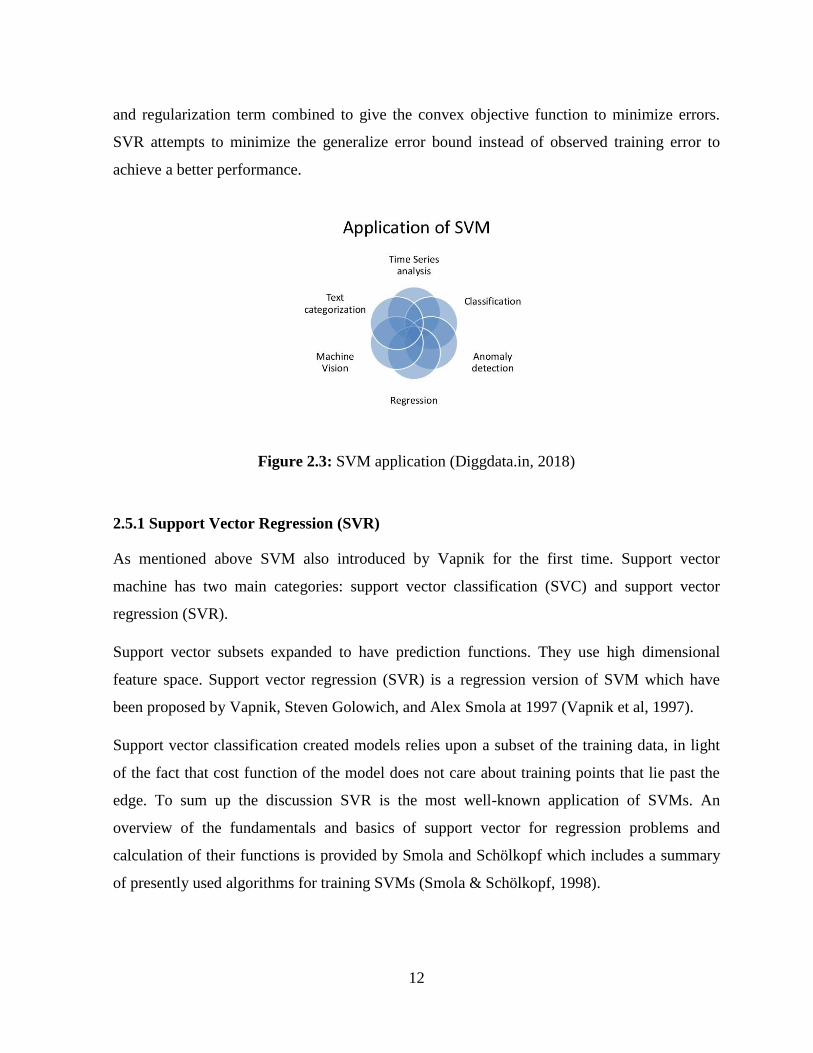
Figure 2.3: SVM application (Diggdata.in, 2018)
2.5.1 Support Vector Regression (SVR)
As mentioned above SVM also introduced by Vapnik for the first time. Support vector
machine has two main categories: support vector classification (SVC) and support vector
regression (SVR).
Support vector subsets expanded to have prediction functions. They use high dimensional
feature space. Support vector regression (SVR) is a regression version of SVM which have
been proposed by Vapnik, Steven Golowich, and Alex Smola at 1997 (Vapnik et al, 1997).
Support vector classification created models relies upon a subset of the training data, in light
of the fact that cost function of the model does not care about training points that lie past the
edge. To sum up the discussion SVR is the most well-known application of SVMs. An
overview of the fundamentals and basics of support vector for regression problems and
calculation of their functions is provided by Smola and Schölkopf which includes a summary
of presently used algorithms for training SVMs (Smola & Schölkopf, 1998).

13
2.6 Related Studies
Since the review is both in neural networks algorithms and support vector machine, in each
part related papers reviewed as follows.
2.6.1 Neural Networks Related Studies
A study conducted by Vyklyuk et al in 2013 for Forex currency forecasting, they used
knowledge Discovered in Databases (KDD) to construct their neural network model. The
model used 3([25x20x10x3]) structure. This structure had been achieved by trial and error
since there is no standard for efficient results. It reduced the error from 7% to 2%. Historical
data of the USD/EUR currency pair is used for training and testing the model. They believe
two weeks of historical data from 23.04.2012 to 04.05.2012 shows the correlation. (Vyklyuk
et al, 2013) claims that this model can be used for forecasting the forex market while it
mentions although that there are other models that perform better.
Another study conducted by (Rehman et al, 2014), it proposes a model for foreign currency
exchange rates. The Cartesian Genetic programming (CGP) deployed for the forecasting. The
study developed Recurrent Cartesian Genetic Programming evolved Artificial Neural Network
(RCGPANN) to produce high accuracy result. The model used five currency exchange rates
against Australian dollar. According to this study the model accuracy is 98.872% which they
used historical data of 1000 days. According to this study best possible inputs and features
extracted from the stock market. As the market historical data is time series the features are
taken from these data for the model to train.
In 2018, Tsai, et al. conducted a research on deep learning which mostly heard these days.
Deep learning has been used for many problems including image recognition problems like
face detection, object detection, or for self-driving cars to detect cars and roads. The study
trained a model to draw an intuitive conclusion from trading charts according to their
visionary characteristics. The input data of the trading was quantitative that pre-processed and
changed to images. The study used convolutional neural network (CNN), one of deep learning
algorithms to train the model. Many experiments conducted in different architectures and the

14
highest accuracy achieved is 94.81%. Based on the graph images the model can obtain a clear
understanding so it helps clients to build better trading strategies.
In 2018 Dash did a research (Dash, 2018) that portrays a model for currency exchange rate
prediction. The study tested different models on historical data and exchange rate of USD
against three currencies of the market over the period of Jan 2014 to Nov 2017. Three
currency pairs USD/CAD, USD/CHF, and USD/JPY data accumulated to train and test the
models. Researcher claims that all performance improvements techniques implemented.
Among the models Pi-Sigma Neural Network and shuffled frog leaping algorithms combined
together in the study, this model showed the better performance among models being tested in
training, validation, and testing. The evaluation techniques like RMSE is used to identify the
error volume. Though the suggested model for forecasting forex is Pi-sigma-ISFL model.
(Tenti, 1996) proposes Recurrent Neural Networks (RNN) for forecasting the FX market. The
study claims sometimes RNN avoided for fears of time consuming but nevertheless it is a
good approach for time series forecasting. According to this study, the algorithm is applicable
to other markets as well but it is suited for Forex because of the nonlinearity nature and many
regularities on the market.
2.6.2 Fuzzy Related Studies
Another study done by Bahrepour et al in 2011 claims that an adaptive ordered fuzzy time
series can perform well on forex market prediction. Because of the uncertainty in forex market
they believe there is two facet about the proposed model:
1. Since the model partition the universe of discourse, it uses self-organizing map (SOM).
The utility of using SOM is that it acts fast in clustering.
2. Order selection approach which is trying to find the best order estimator. The estimation is
fulfilled by three agents in this model. The agents are Voting agent, Statistical agent, and
emotion or decision making agent. All of these agents affect the process of estimation in
the model.
They believe that the suggested model is more accurate than the two models presented by
others in the past. The result of the evaluation is compared with high-order method and Fuzzy

15
Time Series (FTS) and genetic algorithm. The evaluation results show better performance
comparing to those two separately.
(Tseng et al, 2001) proposes a new model from the combination of two models ARIMA and
fuzzy regression. The study calls it fuzzy regression ARIMA or (FARIMA). According to this
research since ARIMA is limited and requires less observations they combined the fuzzy
regression.
The study claims that the model is forecasting well in the following situations:
Provides the best and worst situations for decision makers
Needs less observations than ARIMA model. Minimum is 50 but preferably should be
higher than 100 observations
The model forecast NT Taiwan dollar against US dollar. The model trained using this data.
According to this research, the confidence interval received is 95% and they claim the result is
more satisfactory than simple ARIMA model.
2.6.3 Support Vector Regression Related Studies
According to Handa & Shrivas two models are tested for forex prediction. These two models
are SVR and RNN. In this study 5 years, weekly historical data of three currency against US
dollar used. These three pairs are INR/USD, EUR/USD and HKD/USD. Feature extraction
technique is used to generate new features from the dataset. Totally six features given to the
models including target or output value. Although 10-fold cross validation is used for dynamic
partitioning of the data to improve the performance of the models. They claim it increases the
performance. The models tried to predict 5 weeks ahead. The study used Matlab for the model
creation and performance evaluation. Three performance measurements considered for
evaluations which are MAD, MAPE and RMSE. The study claims that SVR is performing
better than RNN according to their assessments. The process flow diagram of their work
showed in figure 2.4

16
Figure 2.4: Models process flow
Pujari et al., (2018) also investigate models for currency rate prediction. They investigated
most suggested and updated algorithms and models comparatively to propose the best among
them.
They used three algorithms for their study SVR, LSTM, GRU and within the SVR the study
assessed three models including RBF, linear and polynomial.
They collected data of EURO against US dollar from Jan 2017 to Jan 2018 and predicted one
day ahead of the dataset. The performance metrics for their measurements are MSE SMAPE.
Study claims from the SVR models RBF give a closer result rather than linear and polynomial.
In the other hand GRU and LSTM are on par in performance while GRU is more efficient and
less complex than LSTM. To be precise MSE for LSTM and GRU are 0.00009 and 0.00011
while SMAPE is respectively 0.66% and 0.75%.
17
CHAPTER 3
MACHINE LEARNING TECHNIQUES
3.1 Machine Learning
The digital revolution has brought new issues on the table. Fast technology growth, human
interaction with devices and different technologies, electronic records and historic movement
of humans in the internet put hands together to generate a tremendous amount of data every
second. From the past two decades organizations, universities, researchers and academicians
are trying to develop new trends and technologies to utilize these data for different purposes
for instance, for predictions, recognitions, analysis, identifications, recommendations etc.
almost all industries nowadays use machine learning for the enhancement and accuracy of
their working processes and procedures like it is being used in Medical, engineering,
manufacturing, finance etc. one of these trends is Machine learning in computer technology
and artificial intelligence which is considered and targeted by tech experts massively.
The term Machine Learning (ML) is firstly used by Arthur Samuel in 1959 and being
developed and completed with massive other researches till now. ML is part of Artificial
Intelligence (AI) that utilizes statistical methods to give power to computer systems and enable
them to learn from data progressively in the absence of prior instructions and defined
programs (Koza et al, 1996). What ML is doing is that it makes the hidden information know
by evaluating and recognizing patterns and relations between data or events. For these
purposes ML uses computer algorithms, usually, algorithms are built to learn from the data
and make predictions on the same kind of data which is trained by. Traditional applications are
working in limited and restricted instructions which are defined by programmer. Progress and
self-learning properties of algorithms make them overcome traditional applications since
building data driven applications like computer visions or email filtering etc. are almost
infeasible with traditional programming methods. These algorithms help us to take better
decisions and bring reliability. ML has 3 main types they are as follows:

18
Supervised
Unsupervised
Reinforcement
3.1.1 Supervised Learning
In the majority of the cases, supervised learning is used for pragmatic machine learning
problems. There are two variables in supervised learning, one for inputs and one for outputs.
The algorithms are trying to learn mapping between these variables through a mapping
function (Russell & Norvig, 2016). The algorithms are trained with inputs and compared the
result to available outputs. In the training phase as a tutor or teacher, we monitor the learning.
When the algorithm predict the output, it will check whether the answer is right or wrong or
close to output or far from the output. These processes assist the algorithms to learn and
improve their performance. The learning process ends up when it reaches an acceptable
accuracy level. When the new data comes, it tries to predict the output based on the past
learnings and approximate mapping between inputs and outputs.
Supervised learning algorithms are grouped into classification and regression which are
discussed in the last chapter. There are some concerns are exist that these algorithms are only
operational when the data is labeled. Because since the utilizing data as a new oil in the world,
data is not free anymore and gathering data for learning might be costly. For the practical part,
a lot of supervised algorithms have been tested. Each of them had their own strengths and
weaknesses. As a base concept in ML, there is no such algorithm that works best for all kind
of problems. Therefore choosing the algorithm is an important topic that all should consider it
while working in ML. some of the most used supervised algorithms are as follows:
Support Vector Machines
linear regression
logistic regression
naive Bayes
linear discriminant analysis
decision trees

19
Figure 3.1: Supervised Learning model diagram
k-nearest neighbor
Neural Networks
3.1.2 Unsupervised Learning
Unsupervised algorithms unlike supervised do not have correct answers. In other words, there
is no output variable and a guide or teacher to correct mistakes. The algorithms are trying to
understand the data features. They look for hidden and unseen patterns in the dataset to predict
the output by just having the input variables. There are no labels for them to use in order to
learn and improve their predictive ability (OFOR, 2018). Unsupervised learnings are grouped
in clustering and association problems.
Clustering: in this type of problems the data is divided into groups, for instance, grouping
customers by their purchasing behaviors.
Association: algorithms are trying to understand the rules that can clarify the large portion of
the data, for instance, customer buys t-shirt tends to buy pants too.

20
Figure 3.2: Unsupervised learning model diagram
To name a few of unsupervised learning algorithms:
K-means clustering
Apriori algorithm association
3.1.3 Reinforcement Machine Learning
The reinforcement learning basically works like a child learning in the early stage of his/her
life. When a child is doing a good job he or she will be persuaded and when a child is doing a
bad job, the result is somehow punishments or notifying for not repeating that again. These
algorithms are doing the same task by an agent works as a child here. The agent interacts with
environment, it receives reward for performing tasks correctly and penalties for performing it
incorrectly. By the time agent trying to maximize the rewards and minimize the punishments.
Consider a self-driving car, if the car arrived in its destination without any accidents, going out
of the road or bad stops it will receive rewards but if it did any of the mentioned tasks it will
receive penalties. Therefore next time the car will not do the tasks that it took penalties for.
These algorithms are also called dynamic programming and huge amount of studies and

21
Figure 3.3: Reinforcement learning diagram (UCBWiki, 2016)
Researches are being conducted to improve these algorithms, they will be feasible for a lot of
tasks in the near feature.
3.2 Machine Learning Techniques
In this study, the researcher analyzed and deployed 4 supervised algorithms on three pair’s
currency data. Three of these models are from Artificial Neural Networks and one of them is
support vector regression. The techniques are as follows:
Recurrent Neural Network (LSTM)
Radial Basis Function (RBF)
Backpropagation
Support Vector Machine (SVR)
3.2.1 Artificial Neural Networks (ANNs)
ANNs or connectionist networks are invented from the idea of how human brains biological
neural network works. They used to compute and process large amounts of data (Van Gerven
& Bohte, 2018). Usually, inputs are given to neural networks to find or compute appropriate
outputs. The way these networks are functioning is close to human neural networks function,
together to understand the data and provide information for human’s reactions, for instance,
when humans see the fire, the neurons of the eyes send the inputs and collected information
from the scene to the brain. Based on the past information on the brain the desired output
information is generated that it is fire and you should keep yourself away from it to avoid
possible harms. Assume the same with ANNs. Actually, ANN itself is not an algorithm for
doing such tasks. It works as a framework for several ML algorithms and provides tools and

22
techniques that can process a large and complex amount of data or inputs. As mentioned
before, it learns as a child learns in its early stage of life. It learns by examples. Assume an
algorithm that identifies dogs in a lot of different pictures of animals given to it. Since the data
for training the algorithms are labeled in supervised learning, whether the picture is “dog” or
“no dog”. By checking the examples the algorithm identifies the properties, for example, the
dog has a tail, ears, special face of dogs etc. though while giving the new data the neural
network will identify the characteristics and then based on prior knowledge suggest the desired
output. ANN is actually composed of a collection of nodes or units which is originally called
artificial neurons same as we said biological neurons in our brain. These connections are
transferring signals. For instance, one artificial neuron sends a signal to the next one and the
one received the signal can send it to many others with maximum speed that is faster than the
speed of transmission in our brains.
In ANNs the signal between the units are real numbers and output of the ANs are calculated
via non-linear functions which are summing the inputs. As shown in figure 3.4 the vectors or
better to say connections between artificial neurons are usually called ‘edges’. These edges or
from one AN to another AN which consist of one edge has a weight. Weights are used to
adjust the learning procedure by decreasing or increasing the strength of the signals. These
artificial neurons may have thresholds as well to send the signal if the aggregation of the
signals crosses the threshold. There are different layers in ANNs, the first layer is called input
layer where data comes into the network, the data transferring via edges to the next layers
which are usually called hidden layers. And finally, the output layer which presenting the
output after passing the hidden layers and weights adjustments. For the first time, the goal of
ANNs were to function like human brain does, nevertheless by new developments and deep
understanding of the approach it redirected to specific purposes. In the other words different
algorithms and models trained for solving specific problems which it works better than a
general purpose program. It is used for speech recognition, computer visions, medical
diagnoses, filtering spam emails etc.

23
Figure 3.4: ANN elements diagram (Bre, Gimenez, & Fachinotti, 2018)
For further description, a typical artificial neuron illustrated in Figure 3.5. According to Figure
3.5, multiple number of inputs started from 𝑥1, . . . . . 𝑡𝑜 𝑥𝑛 shown by arrows flow the signal
towards a single point which is neuron’s output signal flow (O). The following formula
defines the neuron output signal O (Abraham, 2005).
𝑂 = 𝑓(𝑛𝑒𝑡) = 𝑓 (∑ 𝑤𝑗𝑥𝑗
𝑛
𝑗=1) (3.1)
As you can see in figure 3.5 the 𝑤𝑗 is the weight vector. We also have the 𝑓(𝑛𝑒𝑡) function
which is actually the activation or transfer function. The net variable is the result of weights
multiplies by inputs of the neuron. In the other word, Activation function actually defines the
output of our neuron by those set of inputs entered to our neuron. This procedure continues till
reaching the desired solution or output.
𝑛𝑒𝑡 = 𝑤𝑡𝑥 = 𝑤1𝑥1 + ⋯ + 𝑤𝑛𝑥𝑛 (3.2)
What is new in this formula is t which is the transpose of the matrix. Now to calculate the
output of the neuron O the following should apply:
𝑂 = 𝑓(𝑛𝑒𝑡) = {1 𝑖𝑓 𝑤𝑡𝑥 ≥ 𝜃0 𝑜𝑡ℎ𝑒𝑟𝑤𝑖𝑠𝑒
(3.3)

24
Figure 3.5: Artificial Neuron illustration (Abraham, 2005)
As shown above θ is determining the threshold level. So this type of the nodes are called linear
threshold units (Abraham, 2005).
To conclude this discussion, the main architecture for neuron layers are input, hidden and
output layers. Different signal flows tested for different architectures for instance in feed-
forward networks, there are no feedback connections the signal is coming from the input to the
hidden layers and finally to the output layer in a strictly feed-forward direction while in
contrary of this architecture the Recurrent networks have feedback connections. In these
networks because of the dynamical properties of the networks the activation values play a
significant rule which is reverse in some other architectures. Not to be forgotten, there are
different architectures available for instance, Elman network, adaptive resonance theory maps,
competitive networks, etc. (Abraham, 2005). Now we will discuss the target algorithms in
details.
3.2.1.1 Recurrent Neural Network (LSTM)
For the very first time LSTM was presented by Sepp Hochreiter and Jürgen Schmidhuber in
1997 but after few years it improved by a team under the supervision of the Felix Gers in
1999.
The Long Short-Term Memory units are units of RNN. When the LSTM builds a network of
these units, that network is an LSTM network. The unit built from a cell, an input gate, an
output and a forget gate. The cell and three gates are connected which the cell remembers the

25
value, it means to store the value for a required time interval and those three gates are
regulating the data into and out of the cell. LSTM networks are able to work well with
classifying, processing and prediction of time series data. Traditional RNNs usually had
difficulties dealing with vanishing gradient tasks. This well softness of LSTM with gap length
makes it better over many other algorithms like traditional RNNs, hidden Markova model and
other sequence learning models.
Figure 3.6: LSTM architecture with single cell block
Brief and main forms of LSTM equations are calculate as follows.
𝑓𝑡 = 𝜎𝑔(𝑊𝑓𝑥𝑡+ 𝑈𝑓ℎ𝑡−1 + 𝑏𝑓) (3.4)
𝑖𝑡 = 𝜎𝑔(𝑊𝑖𝑥𝑡+ 𝑈𝑖ℎ𝑡−1 + 𝑏𝑖) (3.5)
𝑜𝑡 = 𝜎𝑔(𝑊𝑜𝑥𝑡+ 𝑈𝑜ℎ𝑡−1 + 𝑏𝑜) (3.6)
𝑐𝑡 = 𝑓𝑡 ⨀ 𝑐𝑡−1 + 𝑖𝑡⨀ 𝜎𝑐(𝑊𝑐𝑥𝑡+ 𝑈𝑐ℎ𝑡−1 + 𝑏𝑐) (3.7)
ℎ𝑡 = 𝑜𝑡⨀𝜎ℎ(𝑐𝑡) (3.8)
In these equations vectors are represented in vectors. Wq and Uq are matrices that contains
weights and recurrent connections. Basically q value is different it can be input gate, output
gate or forget gate or even memory cell based on activation calculation.
xt = input victor ft = forget gate’s activation vector it = input gate’s activation vector ot = output gate’s activation vector

26
ht = output vector ct = cell state vector ⨀ = element-wise product
𝜎𝑔= Sigmoid function
𝜎𝑐 = hyperbolic tangent function
𝜎ℎ= hyperbolic tangent function
3.2.1.2 Radial Basis Function (RBF)
An artificial neural network which is using radial basis functions as their activation functions
is called radial basis function network. A linear combination of radial basis functions of the
inputs and neuron parameters composed the output of the network. These networks used for
function approximation, time series prediction, classification, and system control. RBF
networks proposed by Broomhead and Lowe in 1988 at Royal Signals and Radar
Establishment (Broomhead & Lowe, 1988).
Figure 3.7: RBF structure
As clearly shown in Figure 3.7 RBF has three layers. Started with input layer, a hidden layer,
and a linear output layer with a non-linear RBF activation function. A vector of the real
numbers 𝑥 𝜖 ℝ𝑛 has shaped the input layer. The output which is from the scaled function of
the input vector 𝜑 ∶ ℝ𝑛 → ℝ is taken form:
𝜑(𝑥) = ∑ 𝑎𝑖𝜌(|| 𝑥 − 𝑐𝑖||)𝑁𝑖=1 (3.10)
27
Though N in hidden layer shows the number of neurons, ci is the vector for i neuron, ai is the
weight of the neuron i. Functions are dependent to the distance vector in a radially symmetric
way that is why the name is radial basis function. Usually the inputs are connected to each
hidden neurons. Norms are Euclidean distance and RBF is Gaussian.
𝜌(|| 𝑥 − 𝑐𝑖||) = 𝑒𝑥𝑝[−𝛽|| 𝑥 − 𝑐𝑖||2] (3.11)
The Gaussian basis functions are local to the center vector
lim‖𝑥‖→∞
𝜌(|| 𝑥 − 𝑐𝑖||) = 0 (3.12)
For instance, when we change parameters of one neuron it will have a small effect on input
values which is far from the center of that neuron. RBF acts as universal approximation on
small or compact subset of Rn if some gentle conditions are given for the activation function
(Park & Sandberg, 1991). These clarify that RBF with required hidden neurons is able to
approximate a bounded set of continuous function precisely.
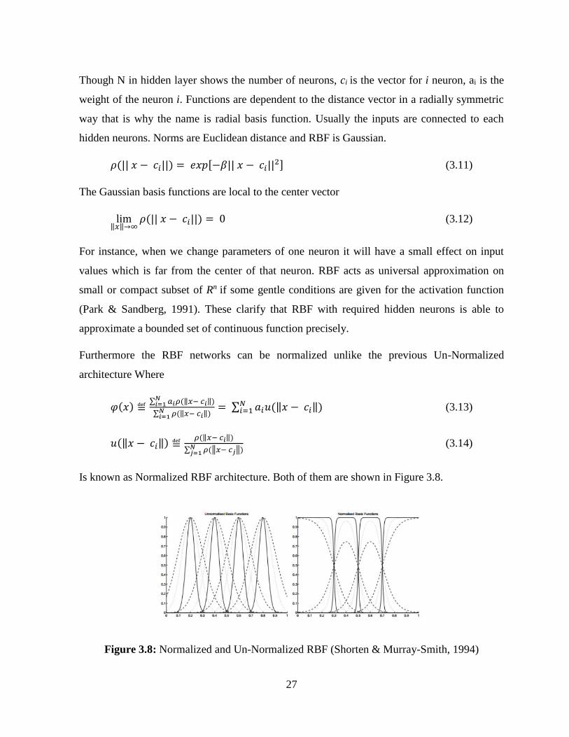
Furthermore the RBF networks can be normalized unlike the previous Un-Normalized
architecture Where
𝜑(𝑥) ≝∑ 𝑎𝑖𝜌(‖𝑥− 𝑐𝑖‖𝑁
𝑖=1 )
∑ 𝜌(‖𝑥− 𝑐𝑖‖𝑁𝑖=1 )
= ∑ 𝑎𝑖𝑢(‖𝑥 − 𝑐𝑖‖)𝑁𝑖=1 (3.13)
𝑢(‖𝑥 − 𝑐𝑖‖) ≝𝜌(‖𝑥− 𝑐𝑖‖)
∑ 𝜌(‖𝑥− 𝑐𝑗‖𝑁𝑗=1 )
(3.14)
Is known as Normalized RBF architecture. Both of them are shown in Figure 3.8.
Figure 3.8: Normalized and Un-Normalized RBF (Shorten & Murray-Smith, 1994)

28
3.2.1.3 Backpropagation
Artificial Neural Network uses weights in the systems to adjust the input and outputs, these
weights are calculated with gradient, Backpropagation is a supervised learning method and
one of the methods to calculate these gradients (Goodfellow et al, 2016). Backpropagation is
derived from “the backward propagation of errors” because usually errors are being calculated
in the output layer then it spread by network layers backwardly. The first layer gradient is
calculated at last since it starts the calculation from the last layer, it uses that value for
recalculation of the previous layers in order and that is the idea of backward methods which
basically form the algorithm. Backpropagation is used for deep learning as well. Basically, it is
part of a bigger structure called automatic differentiation, it is usually used by gradient descent
optimization algorithms to calculate the gradient of the loss function by adjusting the weights
of neurons in the network.
Backpropagation was developed and invented in 1960s by many researchers like Arthur E.
Bryson, Yu-Chi Ho (Nilsson, 1996), and paul werbos in 1974 at US (Werbos, 1974). Finally
at 1986 studies by f David E. Rumelhart, Geoffrey E. Hinton, Ronald J. Williams and James
McClelland (Rumelhart et al, 1986) Gave value to backpropagation and made it popular.
As mentioned a vital task is being done by loss function. Basically, the loss function maps the
values of the variables into numbers which are carrying a cost with it. Specifically, in

29
Figure 3.9: Backpropagation Learning process
Backpropagation, the loss function calculates the difference between the network output and
output itself, the process is completing after the propagate cycle completes.
For the loss function, let’s consider y, yꞌ be vectors in Rn.
To measure the errors or difference between outputs
𝐸(𝑦, 𝑦′) =1
2 ‖𝑦 − 𝑦′‖2 (3.15)
Then the average of losses on n training examples
𝐸 =1
2𝑛 ∑ ‖𝑦(𝑥) − 𝑦′(𝑥)‖2
𝑥 (3.16)
3.2.2 Support Vector Machine (SVR)
Support vector regression is the most commonly used form the SVMs. The SVM which is
usually utilized for classifications but SVR is for regression problems as we discussed briefly
what each of them is doing actually. The SVM is extended from for multipurpose usages. SVR
is one of the usages which makes the computer systems able to work in a regression way over

30
Support vectors. The definition of SVM density estimation utilizes the Structural Risk
Minimization (SRM) guideline, which has been appeared to be better than the customary
Empirical Risk Minimization (ERM) standard utilized in ordinary learning calculations (e.g.
neural networks). A full detail of how SVR is derived is presented by (Smola & Schölkopf,
2004).
Linear SVR
𝑦 = ∑ (𝑎𝑖 − 𝑎𝑖∗)𝑁
𝑖=1 . ⟨𝑥𝑖 , 𝑥⟩ + 𝑏 (3.17)
Figure 3.10: Linear SVR (Sayad, 2017)

31
Nonlinear SVR: The kernel functions transform the data into a higher dimensional feature
space to make it possible to perform the linear separation.
𝑦 = ∑ (𝑎𝑖 − 𝑎𝑖∗)𝑁
𝑖=1 . ⟨𝜑(𝑥𝑖), 𝜑(𝑥)⟩ + 𝑏 (3.18)
𝑦 = ∑ (𝑎𝑖 − 𝑎𝑖∗)𝑁
𝑖=1 . 𝑘⟨𝑥𝑖 , 𝑥⟩ + 𝑏 (3.19)
Figure 3.11: Nonlinear SVR (Sayad, 2017)
Kernel functions:
Polynomial
𝑘(𝑥𝑖 , 𝑥𝑗) = (𝑥𝑖 , 𝑥𝑗) 𝑑 (3.20)
Gaussian Radial Basis function
𝑘(𝑥𝑖 , 𝑥𝑗) = 𝑒𝑥𝑝 (−‖𝑥𝑖−𝑥𝑗‖
2
2𝜎2 ) (3.21)
32
CHAPTER 4
METHODOLOGY
This chapter is designed to describe the methods and tools used to forecast the currency
exchange rates in the Forex market. Firstly the used tools are presented with clarifications of
how they being used within the research. Then the data cleaning, preprocessing and algorithms
are discussed with a brief conclusion and summary of the mentioned issues at the end.
4.1 Tools Used
As of every research this study used some tools for doing experiments and developing
prediction models. Many tools being used for instance the author choose to use python as the
programming language of the model development or historical data of different currencies to
examine their signals or different libraries for which they make us able to use already
implemented algorithms in various massive ways. The following is a brief report of the
manners of these tools.
4.1.1 Python
With so many thanks to Guido van Rossum who created python, it is a general purpose
programming language used for different platforms like web, computer GUI, mathematic and
huge scientific applications. Python is well known by its simplicity, it actually built on bases
of easy programming which is sensitive with blank spaces. Despite that python was built for
kids, nowadays it bits so many strong programming languages in the market. It would not be
unfair if we say it can do whatever you are able to do with every programming language.
Lately, python got popular in the area of artificial intelligence and machine learning because
of its handy bunch of libraries which are growing within developers and experts in this field.
Some of the experts in these fields are coming from economic or other technical backgrounds
though the most convinced programming language that they can start with is python, with its
robustness at the same time.
Basically, the above-mentioned issues and the author’s self-interest caused the models to be
developed in python. Many libraries being used in this study and these are as follows.
33
4.1.1.1 Numpy
This open-source library is doing the computing, it supports multi-dimensional arrays and
matrices with so many functions which make working easy with arrays and matrices. Since
arrays can increase the speed and efficiency in data analysis tasks this library can help a data
scientist a lot. In the forecasting of these data, Numpy is used to store data in arrays. Since the
prediction models require Numpy arrays as their parameters to operate fast and decrease the
training and prediction time.
4.1.1.2 Pandas
This is although an open source library which provides data structures and data analysis tools.
The important note about pandas is its high performance and easy to use especially for
manipulating operations in numerical tables and time series data. Though pandas used to store
the currency data in dataFrame where it then divided in X and Y dimensions and made it ready
for scaling and other preprocessing operations.
4.1.1.3 Matplotlib
Matplotlib is a plotting library that is used to create variety of graphs for different purposes.
The salience of matplotlib is its easiness in use. A good quality plot can be produced with few
lines of code. So matplotlib is used to plot the output historically and also to show the
accuracy and difference between the prediction and real output.
4.1.1.4 Scikit-Learn
Scikit-Learn is another python library which is mostly focused on machine learning. The
library supports different classification, regression and clustering algorithms namely SVM,
Random forest, Gradient boosting, K-means and DBSCAN. It is based on Numpy and SciPy
and interoperates with them fairly. It makes the job of algorithm creation easier for those who
implement those algorithms. In this study Scikit-Learn performed important tasks like scaling
which is normalizing the data between 0 and 1, it dynamically split data into two, train and test
portions. Although, Scikit-Learn is used for calculation of the mean squared error for
performance evaluations.

34
4.1.1.5 Keras & Tensorflow
TensorFlow is also a python library developed by google, for the first it was used internally by
google brain team but then it released open source for the public. Basically, it is for
mathematical operations and also uses widely for machine learning nowadays. TensorFlow
made the implementation of ANNs so easy and convenient for machine learning practitioners.
The Data in Tensorflow is called tensor. These tensors can do a variety of tasks such as
normalization, vectorization or classification (Gerritsen, 2017).
Figure 4.1: A Tensorflow Dataflow Diagram (Abadi et al., 2016)
Keras is also an open source python library which is developed by a google engineer names
François Chollet. It is a special purpose library for neural networks and deep neural networks
for building deep learning models. Its creation is basically on the top of TensorFlow,
Microsoft Cognitive Toolkit or Theano. It is user friendly and fast for implementing
experiments in neural network. The usage is growing and developers use Keras for time saving
and capable functionalities. Not to be forgotten that it is extensible that you can add any
functionality that you think is not included in the package.
Therefore for developing models and experiments for this study, Keras is used for building the
neural network models namely LSTM, RBF, and Backpropagation. Keras has so many built in
functions that are used for developing the study models.
35
4.1.2 Jupyter Notebook
Jupyter Notebook is a web application that provides creation and modification of live codes,
visualizations, equations and plaintexts. This open source notebook supports multiple
programming languages. It uses for numerical simulation, information visualization, machine
learning, statistical modeling, and many more functionalities. The author used this notebook
for writing readable codes for developing models and visualizing the results and accuracy
errors.
4.1.3 Computer
For this research, the computer that is used for training and testing the models has the
following specification: Dell Inspiron 13-5378, 8 GB RAM, Core i7 Quad Core Processor,
Intel HD graphic 4 GB.
4.1.4 Datasets
Three datasets downloaded from dukascopy.com, a Swiss bank which is working in online and
mobile trading. As mentioned in the past chapters since three pairs of currency tested, their
historical data needed. Through the searching in many global active currency exchanger banks
and organizations. Duckascopy provides complete and clean data of our target currency pairs.
The range of the data for two pairs of currency which is EUR/USD and USD/JPY are from 01-
01-2005 to 01-09-2018 with 4992 observations but for the last pair which is USD/TRY the
data is from 13-03-2007 to 01-09-2018 with 4191 observations because of unavailability of the
data. The data is daily which means the currency exchange rate between two currencies in a
daily based; one record for one day. These three datasets have the following attributes which
are used for the forecasting task.
Date
Open
High
Low
Volume
Close
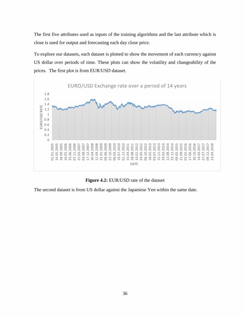
36
The first five attributes used as inputs of the training algorithms and the last attribute which is
close is used for output and forecasting each day close price.
To explore our datasets, each dataset is plotted to show the movement of each currency against
US dollar over periods of time. These plots can show the volatility and changeability of the
prices. The first plot is from EUR/USD dataset.
Figure 4.2: EUR/USD rate of the dataset
The second dataset is from US dollar against the Japaniese Yen within the same date.
0
0.2
0.4
0.6
0.8
1
1.2
1.4
1.6
1.8
01
.01
.20
05
1
6.0
5.2
00
5
28
.09
.20
05
1
0.0
2.2
00
6
25
.06
.20
06
0
7.1
1.2
00
6
21
.03
.20
07
0
4.0
8.2
00
7
17
.12
.20
07
3
0.0
4.2
00
8
12
.09
.20
08
2
5.0
1.2
00
9
09
.06
.20
09
2
2.1
0.2
00
9
06
.03
.20
10
1
9.0
7.2
01
0
01
.12
.20
10
1
5.0
4.2
01
1
28
.08
.20
11
1
0.0
1.2
01
2
24
.05
.20
12
0
6.1
0.2
01
2
18
.02
.20
13
0
3.0
7.2
01
3
15
.11
.20
13
2
9.0
3.2
01
4
12
.08
.20
14
2
5.1
2.2
01
4
09
.05
.20
15
2
1.0
9.2
01
5
03
.02
.20
16
1
7.0
6.2
01
6
30
.10
.20
16
1
4.0
3.2
01
7
27
.07
.20
17
0
9.1
2.2
01
7
23
.04
.20
18
EUR
O/U
SD R
ATE
DATE
EURO/USD Exchange rate over a period of 14 years

37
Figure 4.3: USD/JPY rate of the dataset
And the third dataset which is USD/TRY which has the most falling against US dollar within
the period of 11 years.
Figure 4.4: USD/TRY rate of the dataset
0
20
40
60
80
100
120
140
01
.01
.20
05
16
.05
.20
05
28
.09
.20
05
10
.02
.20
06
25
.06
.20
06
07
.11
.20
06
21
.03
.20
07
04
.08
.20
07
17
.12
.20
07
30
.04
.20
08
12
.09
.20
08
25
.01
.20
09
09
.06
.20
09
22
.10
.20
09
06
.03
.20
10
19
.07
.20
10
01
.12
.20
10
15
.04
.20
11
28
.08
.20
11
10
.01
.20
12
24
.05
.20
12
06
.10
.20
12
18
.02
.20
13
03
.07
.20
13
15
.11
.20
13
29
.03
.20
14
12
.08
.20
14
25
.12
.20
14
09
.05
.20
15
21
.09
.20
15
03
.02
.20
16
17
.06
.20
16
30
.10
.20
16
14
.03
.20
17
27
.07
.20
17
09
.12
.20
17
23
.04
.20
18
USD
/JP
Y R
ATE
DATE
USD/JPY Exchange rate over period of 14 years
0
1
2
3
4
5
6
7
8
12
.03
.20
07
05
.07
.20
07
27
.10
.20
07
18
.02
.20
08
11
.06
.20
08
03
.10
.20
08
25
.01
.20
09
19
.05
.20
09
10
.09
.20
09
02
.01
.20
10
26
.04
.20
10
18
.08
.20
10
10
.12
.20
10
03
.04
.20
11
26
.07
.20
11
17
.11
.20
11
10
.03
.20
12
02
.07
.20
12
24
.10
.20
12
15
.02
.20
13
09
.06
.20
13
01
.10
.20
13
23
.01
.20
14
17
.05
.20
14
08
.09
.20
14
31
.12
.20
14
24
.04
.20
15
16
.08
.20
15
08
.12
.20
15
31
.03
.20
16
23
.07
.20
16
14
.11
.20
16
08
.03
.20
17
30
.06
.20
17
22
.10
.20
17
13
.02
.20
18
07
.06
.20
18
USD
/TR
Y R
ATE
DATE
USD/TRY Exchange rate over the period of 11 years.

38
4.2 Data Preprocessing
For training an algorithm in machine learning we need to clean and prepare the data to be fit
and can be used for training. This preprocessing has many steps which some of them are
different from one approach to another. At the meantime, some of these steps are common
between all. The preprocessing actions conducted for this research are as follows.
The first column of data was timestamp that includes both the date and time which the
observation is taken. The timestamp is splitted in two columns of time and Date, then the
time is removed since this forecasting is daily based not in a timely manner.
Then for making sure of the non-existence of the null values, all columns checked which
the “Volume” had ‘0’ values for Saturday and Sunday of the week. Because the shared
market value of the market is not clear for these two days of the week. Since those two
days were also important for analysis the ‘0’ value cells filled with their above
observations which is one day before that day.
For the feeding purpose in neural network, the data should be in floating points in tensors
(Chollet, 2017). Usually, the good practice is to normalize/scale the data within a specific
range which is mostly from 0 to 1 because data must not be in widely different ranges, it
basically could affect the training negatively. In this study, the data of all attributes
normalized or scaled within this range. The “MinMaxScalr” object is used from Scikit-
Learn library. It basically takes the maximum value of a column as 1 and the minimum
value of the column as 0 and fit other values based on that. The formula for that is as
follows:
𝑧𝑖 = 𝑥𝑖−min (𝑥)
max(𝑥)−min (𝑥) (4.1)
This formula is at the backend which the library provides the facility to normalize the data
much easier.
Data is splitted into two parts, training and testing. Training portion is 80% and the testing
portion is 20% which is a common practice. It starts from 60% training and 40% testing
and goes to a much greater training portion. For this purpose, the “train_test_split” object
of Scikit-Learn is used to randomly divide data based on K-Fold Cross validation
technique.

39
4.3 Algorithms Overview
Since the completion of the data cleaning and preprocessing the training, testing and
visualization come on the table. The cleaning processes were the same for the targeted
algorithms but the rest is a little bit different from one to another. But the road map is the same
for all of them especially for neural network algorithms.
4.3.1 Training, Testing, and Validation
While working on algorithms to monitor the model accuracy the data should separate into
training, testing and validations sets. The training set is used for the learning process which the
algorithm learn the signals of the training examples, the correlation between inputs, their
weights and the output. As described earlier the dataset should be divided into two parts in
cross-validation, though the testing portion is kept aside for testing the accuracy of the model
after it is trained. Though in this study based on most common practices the data is divided
into 80% for training and 20% for testing. The first training is conducted in the training part,
the models are trained based on the examples in this portion. Many techniques have been used
for improving the learning process. Two activation functions “Relu” and “Sigmoid” is tested.
Since the “sigmoid” gave a better result, it is used as activation function. meanwhile different
number of “epochs” and “batch_size” is examined to find the best possible values for these
parameters in order to retrieve a good accuracy and results from the training which ends
mostly same for testing as well.
Despite those efforts, three performance evaluation techniques are used to calculate and
evaluate our models. These three techniques are “RMSE”, “MAE” and “MSE”. The advantage
of these techniques are not just finding the accuracy but at the same time, they make us able to
compare the algorithms and claim which one provides the most accurate result. Based on the
result of the accuracy evaluation techniques, the algorithms compared with each other which is
described in details in Chapter 5.
4.3.2 Visualization
With a simple definition, visualization is the most convenient way of communicating a
message. This has been heard too much that a picture worth thousands of words. Since

40
visualization is also creating images, graphs, and visionary shapes, it makes it easy to make
complex topics easy for understanding. Therefore, in this study, visualization is used for
clarification of the learning process and the accuracy improvement in training phase. In
addition both the actual values which is the real output is comparatively visualized with
predicted output to show the difference in very precise and clear sight. Matplotlib from python
libraries is used for doing this helpful task.
4.4 Model Development Summary
The steps for completing the entire process is described in details. Each step should be done in
a specific time and order to develop a complete and reliable model for currency exchange rate
forecasting. A flow diagram of the entire process is shown in figure 4.5.
Figure 4.5: Entire process flow diagram

41
CHAPTER 5
RESULTS AND DISCUSSION
5.1 Experimental Setup
Few options are available when you are going to implement machine learning algorithms. The
most popular tools are MATLAB, Python, and R programming language. Due to the rich
availability of libraries in python and easiness of use the researcher chooses to use python in
this study. The details of the tools and techniques are presented in Chapter 4. Libraries like
Scikit-Learn, Pandas, Numpy, matplotlib, and Keras are used to carry out amazing
functionalities and are used to process data, create models and visualize data properly. This
chapter describes the model creation and results of the algorithms being used in this study. The
results and evaluation will be presented for 3 neural network models and SVR. Finally a
comparison between the results of each algorithm and at the same time the best model among
them is presented as well.
5.2 Neural Network Algorithms
The study includes 4 models, which 3 of the models are neural network models. The procedure
in each model starts with importing data with pandas, since the powerfulness of pandas for
processes and data preprocessing. Meanwhile, the input and outputs are defined which 4
attributes used as inputs and one attribute which is “close” price of the currency is set as the
output for the models. Additionally, data is splitted into two parts in order with 80% for
training and 20% testing. Finally, the models are created using Keras which is working on
TensorFlow with input, output and 4 hidden layers. The prediction and evaluation conducted
after the training.
5.2.1 Backpropagation
Backpropagation is one of the neural network models which have been used a lot since then.
Based on its popularity and some good performance results in some time series data in the past
by multiple researchers caused to be selected as one of the models for currency rate prediction.

42
As the procedure described above the structure of the Backpropagation of the model is noted
in Table 5.1 for clarifications because the best result achieved after a long process of trial and
errors.
Table 5.1: Backpropagation training parameters
Parameters Values
Number of Epochs 200
Training Method Adam
Loss 0.0001659
Hidden Layer Activation Function Relu
Hidden Layer Activation Function Relu
Hidden Layer Activation Function Relu
Hidden Layer Activation Function Relu
Hidden Layer Activation Function Sigmoid
Dropout percentage 0.2
These parameters being used for the training of the models. Different values have been tested
and the best ones among them selected. After training the model, the performance evaluation
techniques implemented to measure the accuracy of training and testing separately. Needed to
mention that since the model is tested with three pairs of currencies, the evaluation results are
different from currency to another that each of them has different movements and impact
factors in the global market. The results of the EUR/USD, USD/JPY and USD/TRY currency
pairs are presented in Table 5.2, Table 5.3 and Table 5.4.
Table 5.2: EUR/USD training and testing evaluation results with Backpropagation
Training Testing
Parameter Value Parameter Value
Number of observations 3993 Number of observations 999

43
Number of Errors 660 Number of Errors 162
MSE 0.000089 MSE 0.000091
RMSE 0.009446 RMSE 0.009515
MAE 0.007612 MAE 0.007529
Table 5.3: USD/JPY training and testing evaluation results with Backpropagation
Training Testing
Parameter Value Parameter Value
Number of observations 3993 Number of observations 999
Number of Errors 785 Number of Errors 185
MSE 0.000115 MSE 0.000110
RMSE 0.010741 RMSE 0.010477
MAE 0.008731 MAE 0.008545
Table 5.4: USD/TRY training and testing evaluation results with Backpropagation
Training Testing
Parameter Value Parameter Value
Number of observations 3352 Number of observations 839
Number of Errors 1632 Number of Errors 416
MSE 0.000055 MSE 0.000056
RMSE 0.007398 RMSE 0.007464
MAE 0.005992 MAE 0.005984
The model worked well for the prediction purpose, it gives an acceptable result which can be
used as a model to predict the future close rate of these currency pairs. To make it more
understandable that how much the model is able to forecast these, better sightseeing is
visualized in Figure 5.1, Figure 5.2 and Figure 5.3 to show how close or far the prediction and
the real values are.
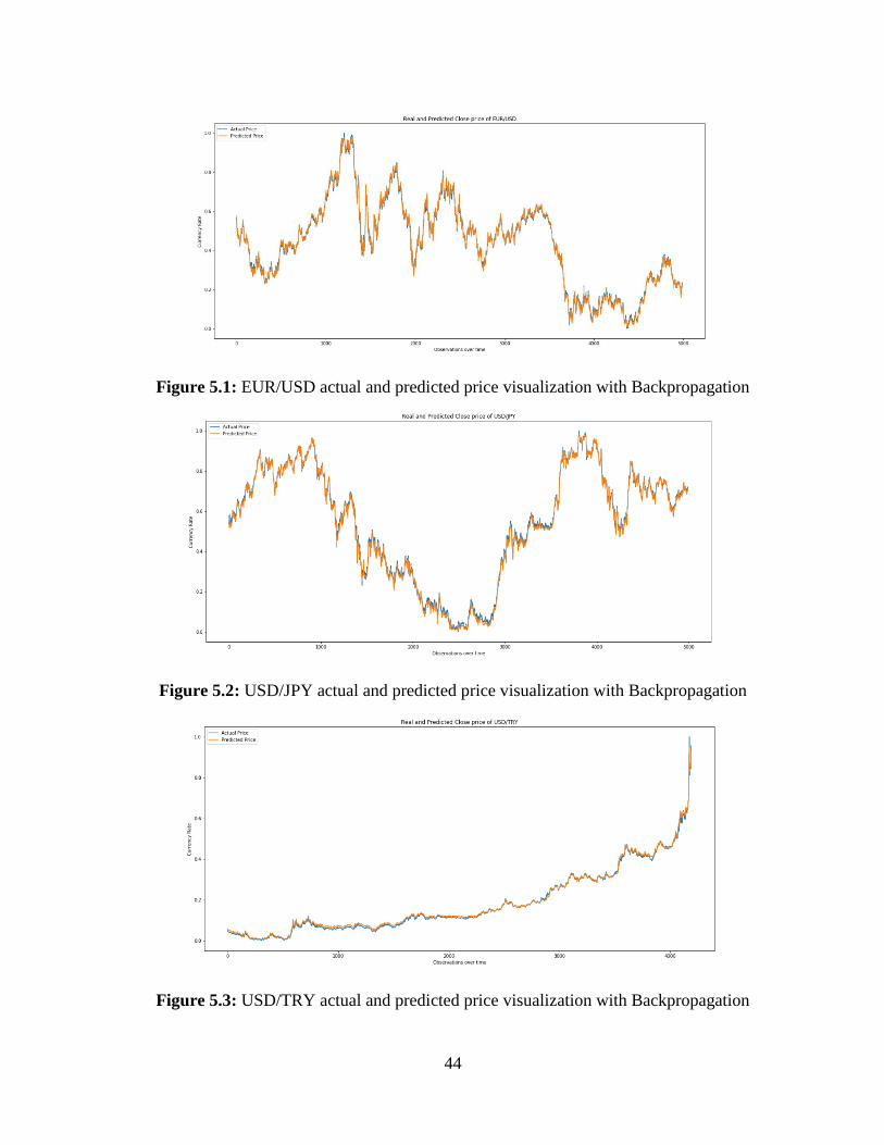
44
Figure 5.1: EUR/USD actual and predicted price visualization with Backpropagation
Figure 5.2: USD/JPY actual and predicted price visualization with Backpropagation
Figure 5.3: USD/TRY actual and predicted price visualization with Backpropagation
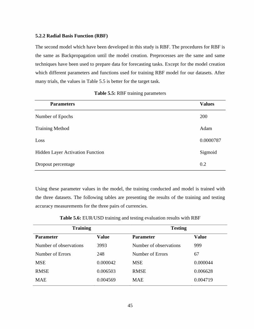
45
5.2.2 Radial Basis Function (RBF)
The second model which have been developed in this study is RBF. The procedures for RBF is
the same as Backpropagation until the model creation. Preprocesses are the same and same
techniques have been used to prepare data for forecasting tasks. Except for the model creation
which different parameters and functions used for training RBF model for our datasets. After
many trials, the values in Table 5.5 is better for the target task.
Table 5.5: RBF training parameters
Parameters Values
Number of Epochs 200
Training Method Adam
Loss 0.0000787
Hidden Layer Activation Function Sigmoid
Dropout percentage 0.2
Using these parameter values in the model, the training conducted and model is trained with
the three datasets. The following tables are presenting the results of the training and testing
accuracy measurements for the three pairs of currencies.
Table 5.6: EUR/USD training and testing evaluation results with RBF
Training Testing
Parameter Value Parameter Value
Number of observations 3993 Number of observations 999
Number of Errors 248 Number of Errors 67
MSE 0.000042 MSE 0.000044
RMSE 0.006503 RMSE 0.006628
MAE 0.004569 MAE 0.004719

46
Table 5.7: USD/JPY training and testing evaluation results with RBF
Training Testing
Parameter Value Parameter Value
Number of observations 3993 Number of observations 999
Number of Errors 322 Number of Errors 85
MSE 0.000046 MSE 0.000048
RMSE 0.006812 RMSE 0.006911
MAE 0.005340 MAE 0.005413
Table 5.8: USD/TRY training and testing evaluation results with RBF
Training Testing
Parameter Value Parameter Value
Number of observations 3352 Number of observations 839
Number of Errors 1169 Number of Errors 300
MSE 0.000028 MSE 0.000034
RMSE 0.005270 RMSE 0.005854
MAE 0.004098 MAE 0.004309
For more clearance and to visualize the forecasting accuracy, the predicted and real values of
the currency prices are plotted in the following figures.

47
Figure 5.4: EUR/USD actual and predicted price visualization with RBF
Figure 5.5: USD/JPY actual and predicted price visualization with RBF
Figure 5.6: USD/TRY actual and predicted price visualization with RBF

48
5.2.3 Long Short-Term Memory (LSTM)
LSTM is one of the RNN models which has been shown great results for most of the time
series data. Based on the literature review the most suggested model for time series data was
LSTM. Based on that the researcher implemented LSTM with these datasets to examine the
result and check whether it gives a fair accuracy or not. Selected parameter values of LSTM is
presented in Table 5.9.
Table 5.9: LSTM training parameters
Parameters Values
Number of Epochs 200
Training Method Adam
Loss 0.0001348
Hidden Layer Activation Function Sigmoid
Dropout percentage 0.2
The performance evaluation results for three datasets is shown in the following tables.
Table 5.10: EUR/USD training and testing evaluation results with LSTM
Training Testing
Parameter Value Parameter Value
Number of observations 3993 Number of observations 999
Number of Errors 531 Number of Errors 129
MSE 0.000082 MSE 0.000082
RMSE 0.009058 RMSE 0.009081
MAE 0.007257 MAE 0.007159
Table 5.11: USD/JPY training and testing evaluation results with LSTM

49
Training Testing
Parameter Value Parameter Value
Number of observations 3993 Number of observations 999
Number of Errors 742 Number of Errors 174
MSE 0.000134 MSE 0.000134
RMSE 0.011595 RMSE 0.011587
MAE 0.009195 MAE 0.009135
Table 5.12: USD/TRY training and testing evaluation results with LSTM
Training Testing
Parameter Value Parameter Value
Number of observations 3352 Number of observations 839
Number of Errors 603 Number of Errors 158
MSE 0.000020 MSE 0.000028
RMSE 0.004526 RMSE 0.005320
MAE 0.003526 MAE 0.003624
Like previous models, the visualization of LSTM from its actual values and predicted values
are plotted to show the accuracy precisely.

50
Figure 5.7: EUR/USD actual and predicted price visualization with LSTM
Figure 5.8: USD/JPY actual and predicted price visualization with LSTM
Figure 5.9: USD/TRY actual and predicted price visualization with LSTM

51
5.3 Support Vector Regression (SVR)
SVR as the name define is from the support vector family. It is the regression of support
vector which is although highly suggested by many researchers for regression problems. Since
other models were from neural network the author tried to examine another model which is not
in that specific category. After evaluations and literature review SVR is selected based many
experiments. Therefore, SVR is also tested with mentioned datasets, the accuracy is measured
and at the same time the result is visualized at the end. The procedure for SVR is the same for
data processing. Same techniques used to prepare data for forecasting tasks. But in training
performance improvement, SVR provides a better solution to choose values for parameters.
Best_estimator object function provides this opportunity to choose values based on the data
being used for forecasting. Therefore, that function is used to find best values. Meanwhile,
SVR has four kernels; linear, Rbf, Sigmoid, and poly. All of them are tested and finally, the
Rbf kernel gave better results among others. Table 5.13 shows the values for different
parameters of the SVR model.
Table 5.13: SVR training parameters
Parameters Values
Kernel rbf
Gamma 0.005
Epsilon 0.01
C 100
Based on these values the model is trained and tested which the results are presented in the
following tables.

52
Table 5.14: EUR/USD training and testing evaluation results with SVR
Training Testing
Parameter Value Parameter Value
Number of observations 3993 Number of observations 999
Number of Errors 171 Number of Errors 39
MSE 0.000026 MSE 0.000027
RMSE 0.005095 RMSE 0.005236
MAE 0.003326 MAE 0.003433
Table 5.15: USD/JPY training and testing evaluation results with SVR
Training Testing
Parameter Value Parameter Value
Number of observations 3993 Number of observations 999
Number of Errors 131 Number of Errors 29
MSE 0.000022 MSE 0.000024
RMSE 0.004678 RMSE 0.004948
MAE 0.003247 MAE 0.003332
Table 5.16: USD/TRY training and testing evaluation results with SVR
Training Testing
Parameter Value Parameter Value
Number of observations 3352 Number of observations 839
Number of Errors 715 Number of Errors 215
MSE 0.000012 MSE 0.000010
RMSE 0.003476 RMSE 0.003141
MAE 0.002534 MAE 0.002618
And the visualization of these results in SVR.

53
Figure 5.10: EUR/USD actual and predicted price visualization with SVR
Figure 5.11: USD/JPY actual and predicted price visualization with SVR
Figure 5.12: USD/TRY actual and predicted price visualization with SVR

54
5.4 Comparison and the Best Model among the Models
The results of tested models for three pairs of currencies presented in details each has good
and bad results in different situations. For instance, for EUR/USD and USD/JPY RBF
performed well than Backpropagation and LSTM but less than SVR which performed best in
all cases. But in USD/TRY the LSTM is performed better than RBF and Backpropagation but
again not as much good as SVR. To conclude the discussion better to evaluate and compare
their performance in a visionary way.
Figure 5.13: Error Comparison of the models
As clearly shown in Figure 5.13, SVR performed better than three other models. And the
values for MSE, RMSE, and MAE which are error measurement techniques shows that SVR
had less errors compared to others. At the same time, RBF is worked better than the other two
models and the backpropagation is the last one.
55
CHAPTER 6
CONCLUSION AND RECOMMENDATIONS
Growing economies in parallel to the rapid strong technology improvements brought the needs
for forecasting in almost every industry. Whether it is customer based marketing, car demands,
mobile devices or currency exchange rate. Currency exchange rate forecasting became a
challenge for human beings. Almost everybody’s economy directly or indirectly connected to
foreign currency prices. Therefore, currency exchange is vital for humans in this era. Machine
learning and generally artificial intelligence technologies going to help humans predict
currency rates. This study developed four models to forecast three pair currency prices in
Forex market comparatively. The models are worked well. More suggested Models were
selected based on literature review. Which the SVR outperformed other three models and
Backpropagation in neural network performed least than others. The procedure is described in
details, from head to tail.
The model’s performance were great due to rich data on the training phase. But the fact that
different factors still remains which the currency rate has many aspects thus forecasting only
time series and historical data is good but not enough. The volatility property of rates are
affected by those factors. The limitation of this study was not considering those factors which
likely to be received from financial and political news of the media.
6.1 Future Works
Since the limitation for the study which is mentioned earlier is crucial, resolving those
challenges would be a great help for improving the accuracy and reliability of the result of this
study. Therefore, the first future work can be a combination of historical data with daily
financial and political news analysis with Natural Language Processing (NLP) models.
The second suggestion for accuracy and reliability improvements is to analyze the factors
which are mentioned in last chapters and examine whether collecting the data from those
factors which affects the currency prices directly can be combined with historical data or not.
How would be the accuracy if some futures of those factors combine with historical data in

56
order to train and test the algorithms based on them. According to believe of the author they
will have crucial impacts on the result if the extraction and collection of data conduct precisely
and accordingly.
Reaching to the point of predicting the currency exchange rate does not look impossible.
According to the author’s believe machine learning will be able to predict currency rate
precisely soon. The impact would be, if the technology is handed to the world business
leaders, the gap between the societies will increase rapidly as it did somehow. But there is one
hope that each technology that humans invent is able to control itself and balance the damages
and its usefulness.

57
REFERENCES
Abadi, M., Barham, P., Chen, J., Chen, Z., Davis, A., Dean, J.… Brain, G. (2016).
TensorFlow: A System for Large-Scale Machine Learning. In Proceedings of the 12th
USENIX Symposium on Operating Systems Design and Implementation (OSDI ’16) (pp.
265–283). Savannah,GA.
Abraham, A. (2005). Artificial neural networks. Handbook of measuring system design.
Andrew, W. M. and Victor, M. (2003), Handbook of International Banking (London: Edward
Elgar Publishing Limited), 350-358
Bahrepour, M., Akbarzadeh-T, M. R., Yaghoobi, M., & Naghibi-S, M. B. (2011). An adaptive
ordered fuzzy time series with application to FOREX. Expert Systems with
Applications, 38(1), 475-485.
BIS. (2016). Triennial central bank survey: Foreign exchange turnover in April 2016
Monetary and Economic Department.
Basak, D., Pal, S., & Patranabis, D. C. (2007). Support vector regression. Neural Information
Processing-Letters and Reviews, 11(10), 203-224.
Borovykh, A., Bohte, S., & Oosterlee, C. W. (2017). Conditional time series forecasting with
convolutional neural networks. arXiv preprint arXiv:1703.04691.
Bre, F., Gimenez, J. M., & Fachinotti, V. D. (2018). Prediction of wind pressure coefficients
on building surfaces using artificial neural networks. Energy and Buildings, 158, 1429-
1441.
Broomhead, D. S., & Lowe, D. (1988). Radial basis functions, multi-variable functional
interpolation and adaptive networks. Royal Signals and Radar Establishment Malvern
(United Kingdom) (No. RSRE-MEMO-4148).
Chollet, F. (2017). Xception: Deep learning with depthwise separable convolutions. arXiv
preprint, 1610-02357.

58
Dash, R. (2018). Performance analysis of a higher order neural network with an improved
shuffled frog leaping algorithm for currency exchange rate prediction. Applied Soft
Computing, 67, 215-231.
Di, M., & Joo, E. M. (2007, December). A survey of machine learning in wireless sensor
netoworks from networking and application perspectives. In Information,
Communications & Signal Processing, 2007 6th International Conference on (pp. 1-5).
IEEE.
Drucker, H. Burges, C.J.C. Kaufman, L. Smola, A. & Vapnik, V. (1997), “Support vector
regression machines” In M. Mozer, M. Jordan, and T. Petsche, editors, Advances in
Neural Information Processing Systems 9, pages 155-161, Cambridge, MA, MIT Press.
Diego, A., Ildar, B., & Oleksiy, P., (2017) A Survey on Computer Science Techniques in the
FOREX Market: Models and Applications. Research in Computing Science 138. pp. 89–
98; ISSN 1870-4069
Frankel, J.A. & Rose, A.K. (1995). Empirical research on nominal exchange rates. In:
Grossman, G. and Rogoff, K. (editors) (1995). Handbook of International Economics, 3.
Amsterdam: North-Holland, 1689-1729.
Freed, M., & Lee, J. (2013, June). Application of support vector machines to the classification
of galaxy morphologies. In Computational and information sciences (ICCIS), 2013 fifth
international conference on (pp. 322-325). IEEE.
Gerritsen, L. (2017). Predicting student performance with Neural Networks, (May).
Goodfellow, I., Bengio, Y., Courville, A., & Bengio, Y. (2016). Deep learning (Vol. 1).
Cambridge: MIT press.
Goodman, S.H. (1978). Foreign exchange rate forecasting techniques: Implications for
business and policy. The Journal of Finance, 34, 2, 415-427.
Handa, R., & Shrivas, A. K. (n.d) Prediction of forex data using neural network techniques
with feature extraction.

59
Kalghatgi, M. P., Ramannavar, M., & Dr. Sidnal, N. S. (2015). A Neural Network Approach
to Personality Prediction based on the Big-Five Model. International Journal of
Innovative Research in Advanced Engineering, 2(8), 56–63
Khan, K., Baharudin, B. B., & Khan, A. (2009, June). Mining opinion from text documents: A
survey. In Digital Ecosystems and Technologies, 2009. DEST'09. 3rd IEEE International
Conference on (pp. 217-222). IEEE.
Koza, J. R., Bennett, F. H., Andre, D., & Keane, M. A. (1996). Automated design of both the
topology and sizing of analog electrical circuits using genetic programming. In Artificial
Intelligence in Design’96 (pp. 151-170). Springer, Dordrecht.
Lison, P. (2012). An introduction to machine learning. Retrieved from
http://folk.uio.no/plison/pdfs/talks/machinelearning.pdf
Mark, N. C. (1995), "Exchange Rates and Fundamentals: Evidence on Long-Horizon
Predictability," American Economic Review 85 (March): pp. 201-18.
Nguyen, T. T., & Armitage, G. (2008). A survey of techniques for internet traffic classification
using machine learning. IEEE Communications Surveys & Tutorials, 10(4), 56-76.
Nilsson, N. J. (1996). Stuart Russell and Peter Norvig, Artificial Intelligence: A Modern
Approach. Artificial intelligence, 82(1-2), 369-380.
Ofor, e. (2018). Machine learning techniques for immunotherapy dataset
classification (Master dissertation, Near East University).
Park, J., & Sandberg, I. W. (1991). Universal approximation using radial-basis-function
networks. Neural computation, 3(2), 246-257.
Patel, P. J., Patel, N. J., & Patel, A. R. (2014). Factors affecting currency exchange rate,
economical formulas and prediction models. International Journal of Application or
Innovation in Engineering & Management (IJAIEM), 3(3), 53-56.
Pujari, M. V., Sayyed, A. H., Shahani, H., Rupani, D., & Student, B. E. (2018). Forex Trading
System. International Journal of Engineering Science, 17116.

60
Qi, M., & Zhang, G. P. (2008). Trend time–series modeling and forecasting with neural
networks. IEEE Transactions on neural networks, 19(5), 808-816.
Rehman, M., Khan, G. M., & Mahmud, S. A. (2014). Foreign currency exchange rates
prediction using CGP and recurrent neural network. IERI Procedia, 10, 239-244.
Rumelhart, D. E., Hinton, G. E., & Williams, R. J. (1986). Learning representations by back-
propagating errors. nature, 323(6088), 533.
Russell, S. J., & Norvig, P. (2016). Artificial intelligence: a modern approach. Malaysia;
Pearson Education Limited.
Sayad, S. (2017). Support Vector Machine. Support Vector Machines. Np, nd Web, 26.
Schumaker, R. P., & Chen, H. (2009). Textual analysis of stock market prediction using
breaking financial news: The AZFin text system. ACM Transactions on Information
Systems (TOIS), 27(2), 12.
Smola, A.J. & Schölkopf, B. (1998), “A Tutorial on Support Vector Regression”,
NeuroCOLT, Technical Report NC-TR-98-030, Royal Holloway College, University of
London, UK.
Shorten, R., & Murray-Smith, R. (1994, September). On normalising radial basis function
networks. In Proceedings of the fourth Irish Conference on Neural Networks,
INNC (Vol. 94, pp. 213-217).
Smola, A. J., & Schölkopf, B. (2004). A tutorial on support vector regression. Statistics and
computing, 14(3), 199-222.
Tenti, P. (1996). Forecasting foreign exchange rates using recurrent neural networks. Applied
Artificial Intelligence, 10(6), 567-582.
The Federal Reserve Board. (2004) "FRB: Speech, Bernanke--International Monetary Reform
and Capital Freedom--October 14, 2004”.
Tomas, C., (2007) Forecast Accuracy and Biases in Professional FX Rate Predictions.
University of Van Tilburg. Pp. 2-60. 96.96.41.

61
Tsai, Y. C., Chen, J. H., & Wang, J. J. (2018). Predict Forex Trend via Convolutional Neural
Networks. arXiv preprint arXiv:1801.03018.
Tseng, F. M., Tzeng, G. H., Yu, H. C., & Yuan, B. J. (2001). Fuzzy ARIMA model for
forecasting the foreign exchange market. Fuzzy sets and systems, 118(1), 9-19.
UCBWiki. (2016, February). Reinforcement Learning with Function approximation. Retrieved
April 22, 2018, from UCB WIki: http://wiki.ubc.ca/images/b/bd/Rldiagram1.png
Vapnik, V. (1995), “The Nature of Statistical Learning Theory”, Springer Verlag.
Vapnik, V. Golowich, S. & Smola, A. (1997), “Support Vector Method for Function
Approximation, Regression Estimation, and Signal Processing”, in M. Mozer, M. Jordan,
and T. Petsche (eds.), Neural Information Processing Systems, Vol. 9. MIT Press,
Cambridge, MA.
Van Gerven, M., & Bohte, S. (Eds.). (2018). Artificial neural networks as models of neural
information processing. Frontiers Media SA.
Vyklyuk, Y., Vukovic, D., & Jovanovic, A. (2013). FOREX prediction with neural network:
USD/EUR currency pair. Актуальні проблеми економіки, (10), 261-273.
Werbos, P. (1974). Beyond Regression:" New Tools for Prediction and Analysis in the
Behavioral Sciences. Ph. D. dissertation, Harvard University.
Wernick, M. N., Yang, Y., Brankov, J. G., Yourganov, G., & Strother, S. C. (2010). Machine
learning in medical imaging. IEEE signal processing magazine, 27(4), 25-38.
Zamani, M., & Kremer, S. C. (2011, November). Amino acid encoding schemes for machine
learning methods. In Bioinformatics and Biomedicine Workshops (BIBMW), 2011 IEEE
International Conference on (pp. 327-333). IEEE.
Zhang, M.-L. Z. M.-L., & Zhou, Z.-H. Z. Z.-H. (2006). Multilabel Neural Networks with
Applications to Functional Genomics and Text Categorization. IEEE Transactions on
Knowledge and Data Engineering, 18(10), 1–14
Znaczko, T. M. (2013). Forecasting Foreign Exchange Rates.