1ECEN5807 CPM

Current Programmed Control(i.e. Peak Current-Mode Control)

Lecture slides part 2More Accurate Models

ECEN 5807 Dragan Maksimović

2ECEN5807 CPM

Simple First-Order CPM Model: Summary

• Assumption: CPM controller operates ideally, ⟨iL⟩ = ic• Useful results at low frequencies, well suited for conservative

(relatively low bandwidth) design of voltage feedback loop around CPM controlled converter

• Limitations:– The simple model does not indicate possible instability of the current

controller, or the need for a compensation (“artificial”) ramp– Does not include high-frequency dynamics, which is relevant for wide-

bandwidth voltage loop designs– Does not correctly model line-to-output responses in CPM buck or

buck-derived converters even at low frequencies (it incorrectly predicts complete rejection of line disturbances)

3ECEN5807 CPM

More Accurate CPM Models: Outline

• Sampled-data modeling of inductor dynamics in current programmed mode

– Instability of the current loop and the need for compensation (“artificial”) ramp

– Improved modeling of high-frequency dynamics to enable design of wide-bandwidth voltage loops

• More accurate averaged model– Large-signal and small-signal averaged modulator model– Accurate averaged small-signal models, including high-frequency

dynamics– Accurate modeling of line-to-output responses

• Discussion of results for basic converters• CPM model for simulations• Design examples

4ECEN5807 CPM

5ECEN5807 CPM

6ECEN5807 CPM

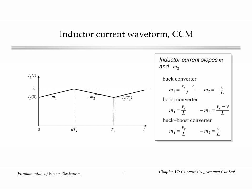
Inductor current in transient

d[n]Ts d’[n]Ts d’[n+1]Tsd[n+1]Ts

ic[n]ic[n+1]

iL(t)

m1(t)−m2(t)

7ECEN5807 CPM

High-frequency small-signal inductor-current dynamics

• Assume that voltage perturbations are negligibly small at high frequencies: the slopes m1 and m2 can be considered constant

• Apply sampled-data modeling:

)(ˆ][ˆ][ˆˆ)(ˆ * tininiiti LLccc →→→→

)(ˆ)(ˆ)(ˆ)(ˆ1)(ˆ sizizijksiT

si LLck

scs

c →→→−→ ∑+∞

−∞=

ω

8ECEN5807 CPM

Small-signal perturbation

ic[n]

m1(t)−m2(t)

ic + ic

iL[n]

d[n]TsiL[n-1]

9ECEN5807 CPM

Discrete-time dynamics ][ˆ][ˆ nini Lc →

sLL Tndmmnini ][ˆ)(]1[ˆ][ˆ21 ++−=

sLc Tndmnini ][ˆ]1[ˆ][ˆ1+−=

10ECEN5807 CPM

Discrete-time dynamics ][ˆ][ˆ nini Lc →

sLL Tndmmnini ][ˆ)(]1[ˆ][ˆ21 ++−=

sLc Tndmnini ][ˆ]1[ˆ][ˆ1+−=

][ˆ)1(]1[ˆ ][ˆ]1[ˆ][ˆ1

21

1

2 nininimmmni

mmni cLcLL αα −+−=

++−−=

'

1

2

1

2

DD

MM

mm

−=−=−=α

11ECEN5807 CPM

Instability for D > 0.5

][ˆ)1(]1[ˆ ][ˆ ninini cLL αα −+−=

'

1

2

1

2

DD

MM

mm

−=−=−=α

12ECEN5807 CPM

13ECEN5807 CPM

14ECEN5807 CPM

15ECEN5807 CPM

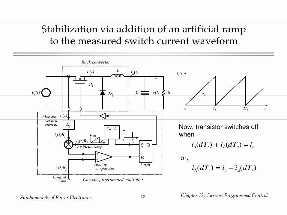
Small-signal perturbation with compensation ramp

ic[n]

m1(t) −m2(t)

ic + ic

iL[n]

d[n]TsiL[n-1]

−ma(t)

16ECEN5807 CPM

Discrete-time dynamics with compensation ramp: ][ˆ][ˆ nini Lc →

sLL Tndmmnini ][ˆ)(]1[ˆ][ˆ21 ++−=

saLc Tndmmnini ][ˆ)(]1[ˆ][ˆ1 ++−=

17ECEN5807 CPM

sLL Tndmmnini ][ˆ)(]1[ˆ][ˆ21 ++−=

][ˆ)1(]1[ˆ ][ˆ]1[ˆ][ˆ1

21

1

2 nininimmmmni

mmmmni cLc

aL

a

aL αα −+−=

++

+−+−

−=

2

2

1

2

'

1

mm

DD

mm

mmmm

a

a

a

a

+

−−=

+−

−=α

Discrete-time dynamics with compensation ramp: ][ˆ][ˆ nini Lc →

saLc Tndmmnini ][ˆ)(]1[ˆ][ˆ1 ++−=

18ECEN5807 CPM

][ˆ)1(]1[ˆ ][ˆ ninini cLL αα −+−=

19ECEN5807 CPM

20ECEN5807 CPM

21ECEN5807 CPM

][ˆ)1(]1[ˆ ][ˆ ninini cLL αα −+−=

Discrete-time dynamics: )(ˆ)(ˆ zizi Lc →

Z-transform: )(ˆ)1()(ˆ )(ˆ 1 zizzizi cLL αα −+= −

1 11

)(ˆ)(ˆ

−−−

=zzi

zi

c

L

ααDiscrete-time (z-domain) control-to-

inductor current transfer function:

ss TjsT ee ωαα

αα

−− −−

→−

− 1

11

1

Difference equation:

• Pole at z = α • Stability condition: pole inside the unit circle, |α| < 1• Frequency response (note that z−1 corresponds to a delay of Ts in

time domain):

22ECEN5807 CPM

Equivalent hold:

ic[n]

m1(t) −m2(t)

ic + ic

iL[n]

d[n]TsiL[n-1]

−ma(t)

)(ˆ)(ˆ ),(ˆ][ˆ sizitini LLLL →→

iL(t) iL[n]

Ts

23ECEN5807 CPM

Equivalent hold

• The response from the samples iL[n] of the inductor current to the inductor current perturbation iL(t) is a pulse of amplitude iL[n] and length Ts

• Hence, in frequency domain, the equivalent hold has the transfer function previously derived for the zero-order hold:

se ssT−−1

24ECEN5807 CPM

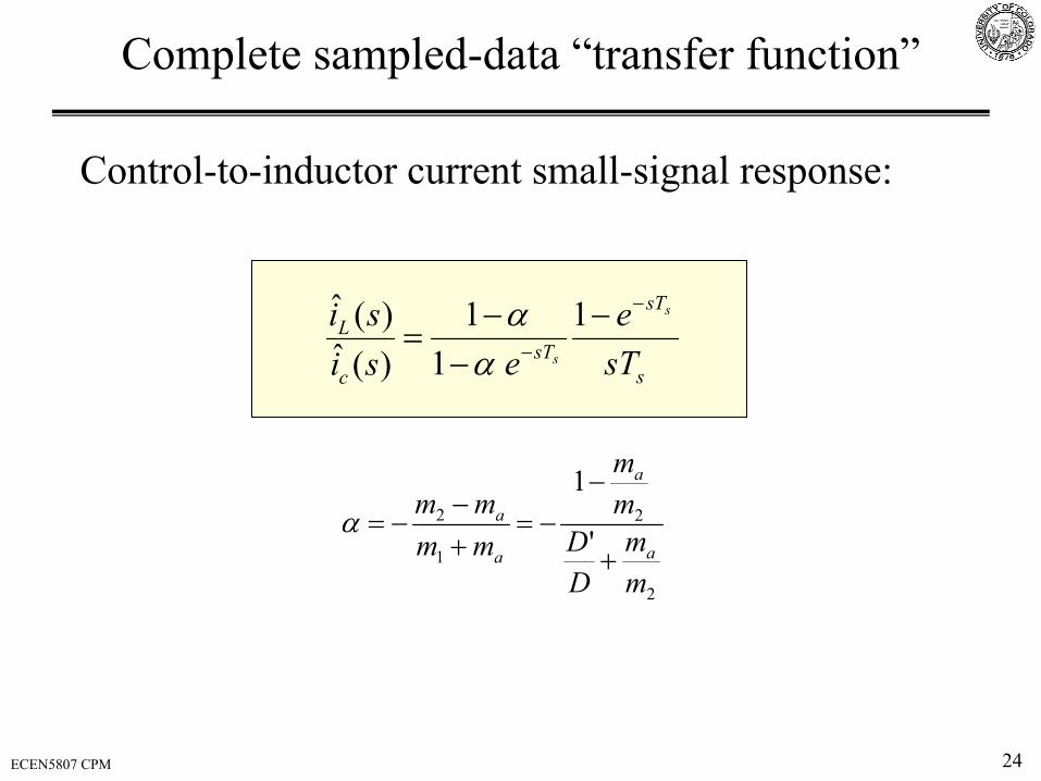
Complete sampled-data “transfer function”

s

sT

sTc

L

sTe

esisi s

s

−

−

−−

−=

1 1

1)(ˆ)(ˆ

αα

2

2

1

2

'

1

mm

DD

mm

mmmm

a

a

a

a

+

−−=

+−

−=α

Control-to-inductor current small-signal response:

25ECEN5807 CPM

Example

• CPM buck converter:Vg = 10V, L = 5 µH, C = 75 µF, D = 0.5, V = 5 V, I = 20 A, R = V/I = 0.25 Ω, fs = 100 kHz

• Inductor current slopes:m1 = (Vg – V)/L = 1 A/µsm2 = V/L = 1 A/µs

2

2

2

2

1

2

1

1

'

1

mmmm

mm

DD

mm

mmmm

a

a

a

a

a

a

+

−−=

+

−−=

+−

−=α

D = 0.5: CPM controller is stable for any compensation ramp, ma/m2 > 0

s

sT

sTc

L

sTe

esisi s

s

−

−

−−

−=

1 1

1)(ˆ)(ˆ

αα

26ECEN5807 CPM

Control-to-inductor current responses for several compensation ramps (ma/m2 is a parameter)

102 103 104 105-40

-30

-20

-10

0

10

20m

agni

tude

[db]

iL/ic magnitude and phase responses

102 103 104 105

-150

-100

-50

0

frequency [Hz]

phas

e [d

eg]

ma/m2=0.1

ma/m2=0.5

ma/m2=1

ma/m2=5

5

10.5

0.1

MATLAB file: CPMfr.m

27ECEN5807 CPM

First-order approximation

hfs

s

sT

sTc

L

sssTe

esisi s

s

ωπωααα

α

+=

−+

+≈

−−

−=

−

−

1

1

)/(111

11 1

1)(ˆ)(ˆ

)/(1

)/(1

πω

πω

s

ssT

s

s

e s

+

−≈−

ππαα s

a

shf

f

mmDD

ff

2

221

111

+−=

+−

=

Control-to-inductor current response behaves approximately as a single-pole transfer function with a high-frequency pole at

28ECEN5807 CPM

Control-to-inductor current responses for several compensation ramps (ma/m2 = 0.1, 0.5, 1, 5)

102 103 104 105-40

-30

-20

-10

0

10

20m

agni

tude

[db]

iL/ic magnitude and phase responses

102 103 104 105

-150

-100

-50

0

frequency [Hz]

phas

e [d

eg]

1st-order transfer-function approximation

29ECEN5807 CPM

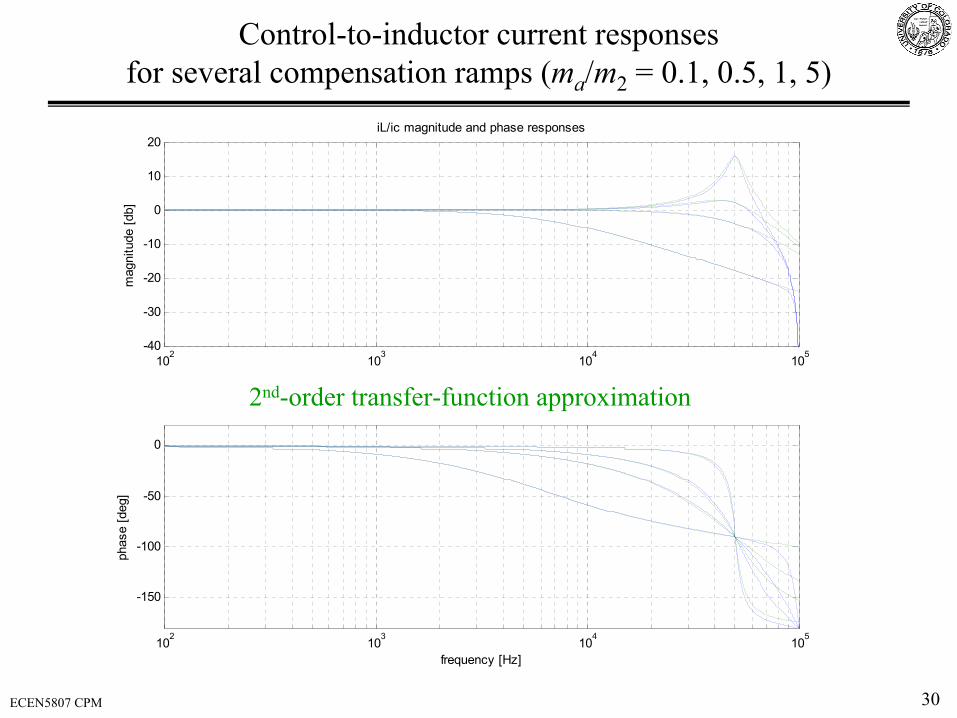
Second-order approximation

2

2/)2/(11

21

11 1

1)(ˆ)(ˆ

+

−+

+

≈−

−−

=−

−

ss

s

sT

sTc

L

sssTe

esisi s

s

ωωααπα

α

2

2

2/)2/(21

2/)2/(21

++

+−

≈−

ss

sssT

ss

ss

e s

ωωπ

ωωπ

2

221

12112

mmDD

Qa+−

=+−

=πα

απ

Control-to-inductor current response behaves approximately as a second-order transfer function with corner frequency fs/2 and Q-factor given by

30ECEN5807 CPM

102 103 104 105-40

-30

-20

-10

0

10

20m

agni

tude

[db]

iL/ic magnitude and phase responses

102 103 104 105

-150

-100

-50

0

frequency [Hz]

phas

e [d

eg]

Control-to-inductor current responses for several compensation ramps (ma/m2 = 0.1, 0.5, 1, 5)

2nd-order transfer-function approximation

31ECEN5807 CPM

Conclusions

• In CPM converters, high-frequency inductor dynamics depend strongly on the compensation (“artificial”) ramp slope ma

• Without compensation ramp (ma = 0), CPM controller is unstable for D > 0.5, resulting in period-doubling or other sub-harmonic (or even chaotic) oscillations

• For ma = 0.5m2, CPM controller is stable for all D• Relatively large compensation ramp (ma > 0.5m2) is a practical choice not just

to ensure stability of the CPM controller, but also to reduce sensitivity to noise

• For relatively large values of ma, high-frequency inductor current dynamics can be well approximated by a single high-frequency pole

• Second-order approximation is very accurate for any ma• Next: more accurate averaged model, including high-frequency dynamics