curve fitting: fertilizer, fonts, and ferraris. what's the difference between modeling and...
TRANSCRIPT

Curve Fitting: Fertilizer, Fonts, and Ferraris
Curve Fitting: Fertilizer, Fonts, and Ferraris
What's the difference between modeling and curve fitting, and what are polynomials used for, anyway?
32nd AMATYC Annual ConferenceNovember 3, 2006Cincinnati, Ohio
Katherine YoshiwaraBruce Yoshiwara
Los Angeles Pierce College
Typical Quadratic Models●Projectile and other motion problems from physics
●Problems involving area or the Pythagorean Theorem
●Revenue curves:Total revenue = (number of items)(price per item)
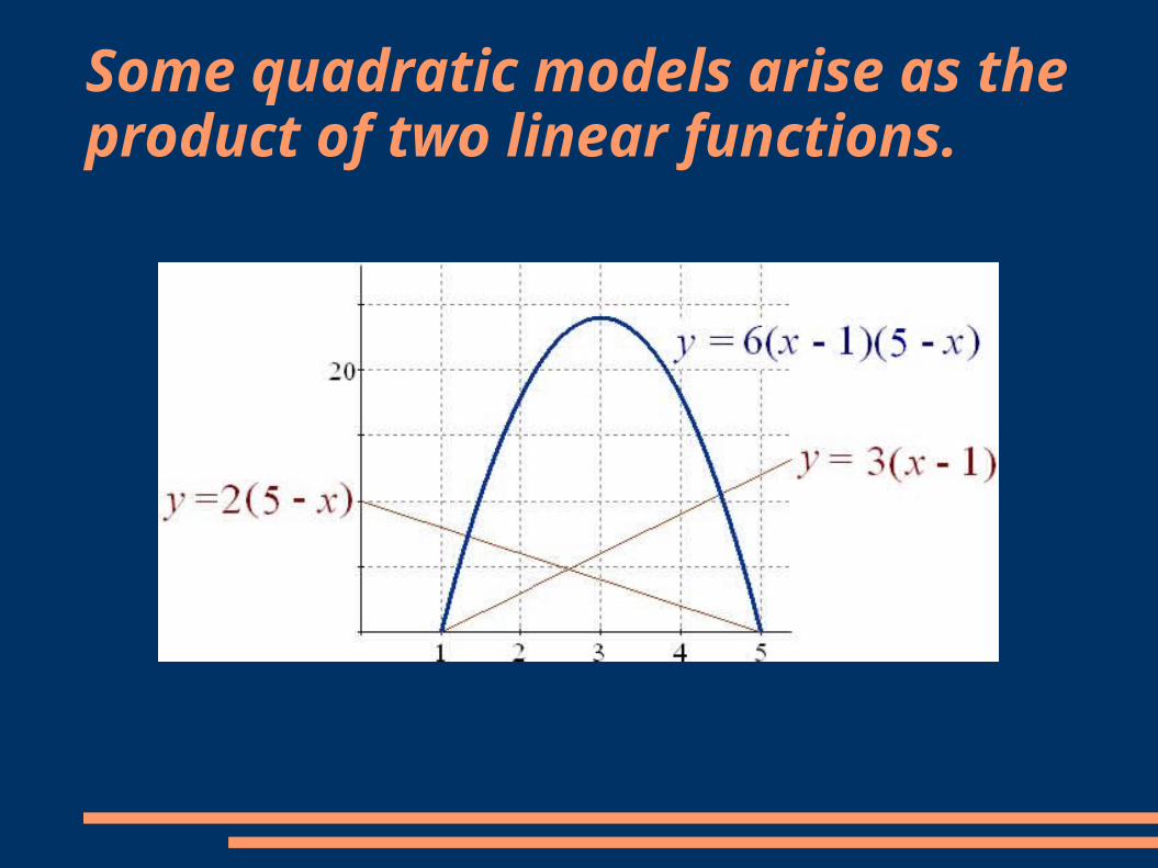
Some quadratic models arise as the product of two linear functions.
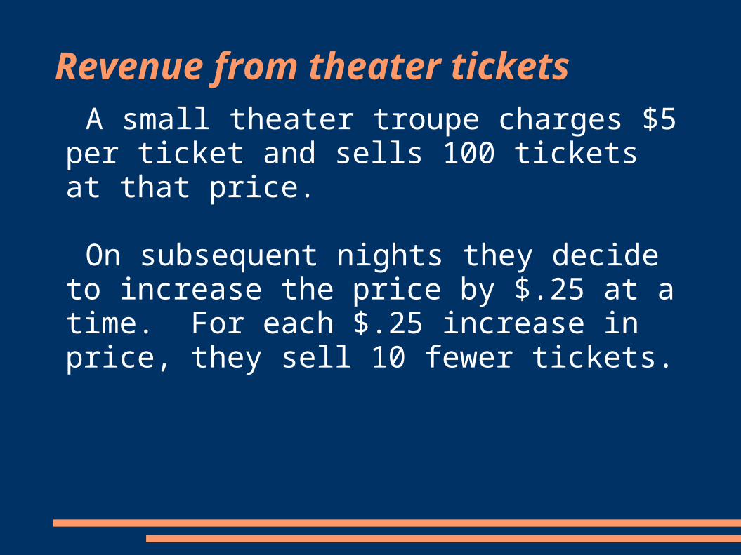
Revenue from theater tickets
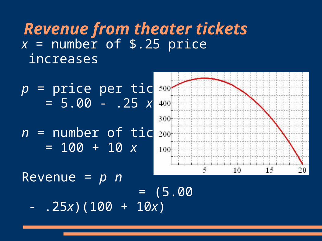
A small theater troupe charges $5 per ticket and sells 100 tickets at that price.
On subsequent nights they decide to increase the price by $.25 at a time. For each $.25 increase in price, they sell 10 fewer tickets.
Revenue from theater tickets
x = number of $.25 price increases
p = price per ticket = 5.00 - .25 x
n = number of tickets = 100 + 10 x
Revenue = p n = (5.00 - .25x)(100 + 10x)
Rate of growth in a logistic model
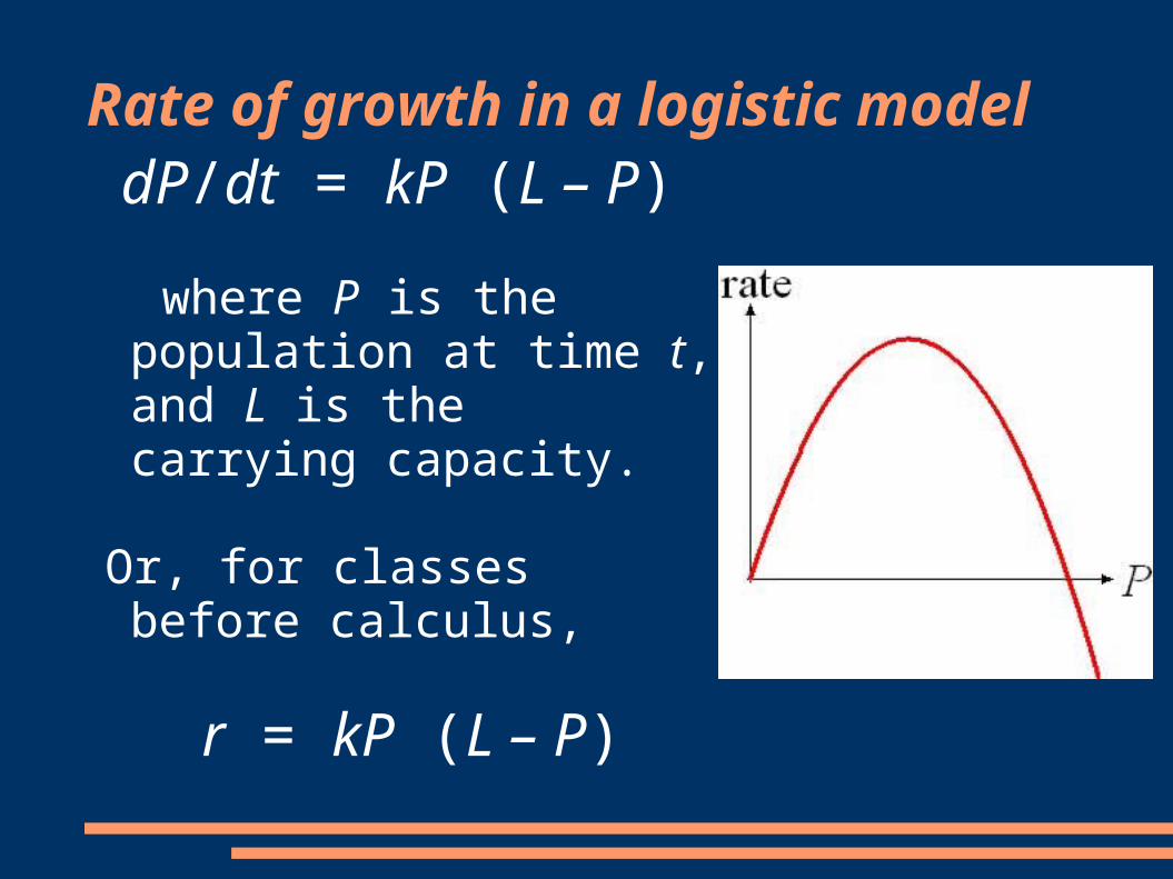
dP/dt = kP (L – P)
where P is the population at time t, and L is the carrying capacity.
Or, for classes before calculus,
r = kP (L – P)

Logistic growth
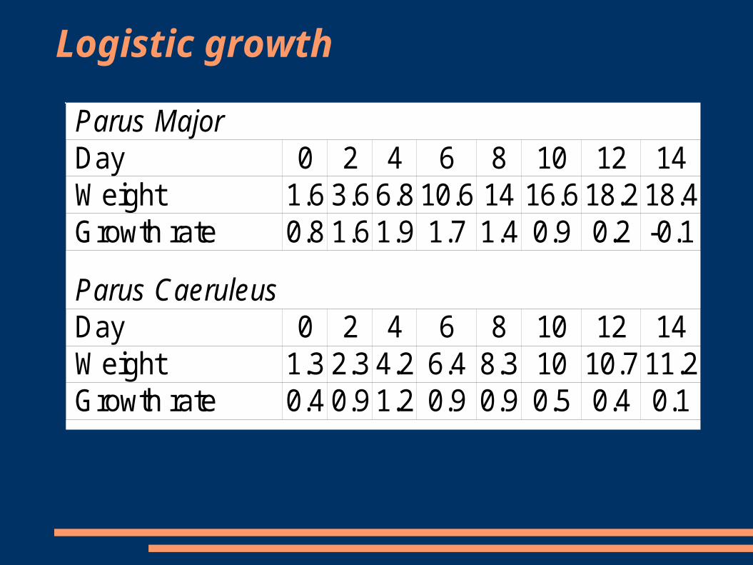
The figure shows the typical weight of two species of birds each day after hatching.
Compute the daily rate of growth for each species.
Logistic growth
Day 0 2 4 6 8 10 12 14 Weight 1.6 3.6 6.8 10.6 14 16.6 18.2 18.4 Growth rate 0.8 1.6 1.9 1.7 1.4 0.9 0.2 -0.1
Day 0 2 4 6 8 10 12 14 Weight 1.3 2.3 4.2 6.4 8.3 10 10.7 11.2 Growth rate 0.4 0.9 1.2 0.9 0.9 0.5 0.4 0.1
Parus Major
Parus Caeruleus
Logistic growth (continued)
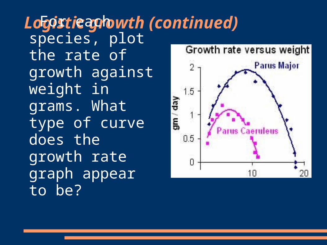
For each species, plot the rate of growth against weight in grams. What type of curve does the growth rate graph appear to be?
Maximum sustainable yield Commercial fishermen rely on a steady supply of
fish in their area. To avoid overfishing, they adjust their harvest to the size of the population. The equation
r = 0.0001x (4000 – x)
gives the annual rate of growth, in tons per year, of a fish population of biomass x tons.
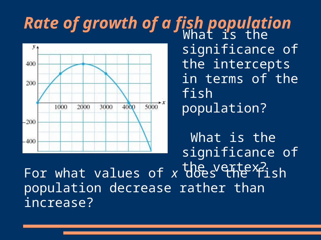
Rate of growth of a fish population
What is the significance of the intercepts in terms of the fish population?
What is the significance of the vertex?
For what values of x does the fish population decrease rather than increase?
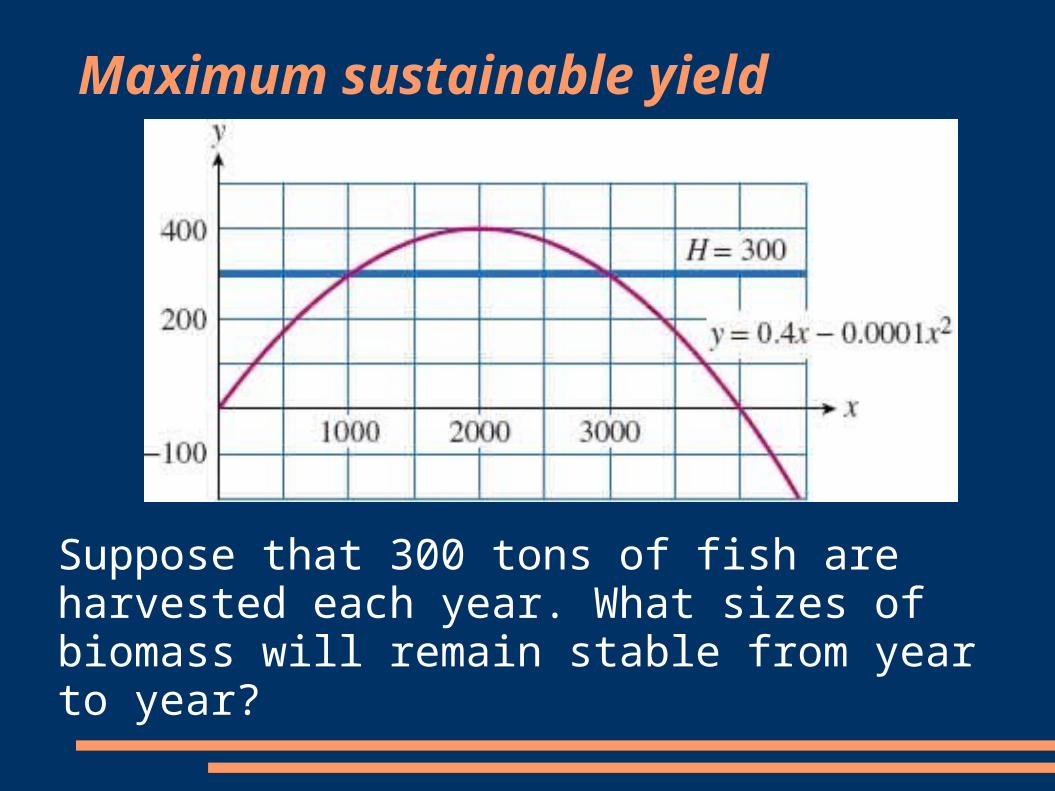
Maximum sustainable yield
Suppose that 300 tons of fish are harvested each year. What sizes of biomass will remain stable from year to year?
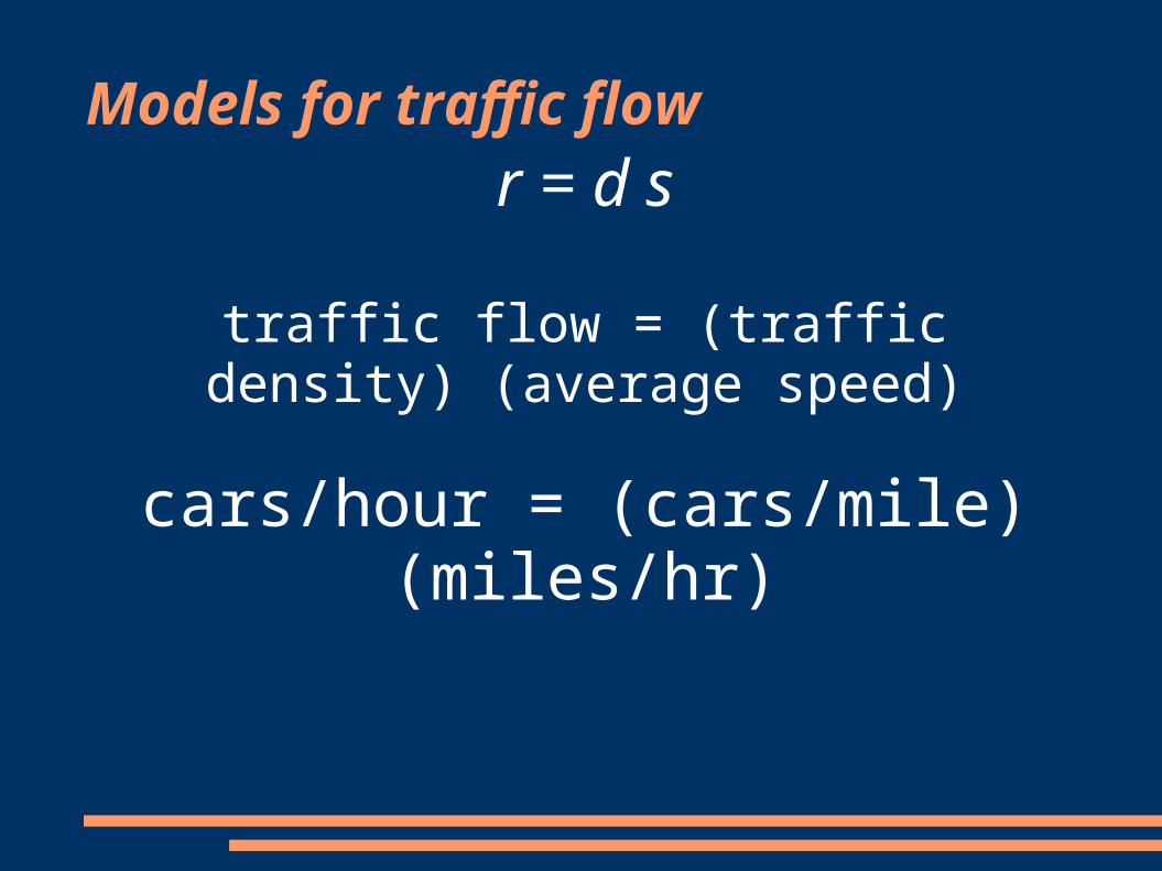
Models for traffic flow
r = d s
traffic flow = (traffic density) (average speed)
cars/hour = (cars/mile) (miles/hr)
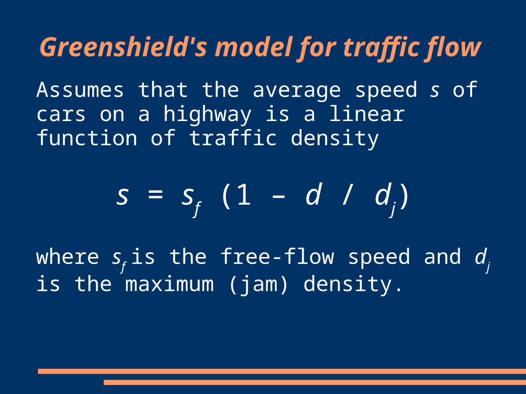
Greenshield's model for traffic flow
Assumes that the average speed s of cars on a highway is a linear function of traffic density
s = sf (1 – d / d
j)
where sf is the free-flow speed and d
j is the maximum
(jam) density.
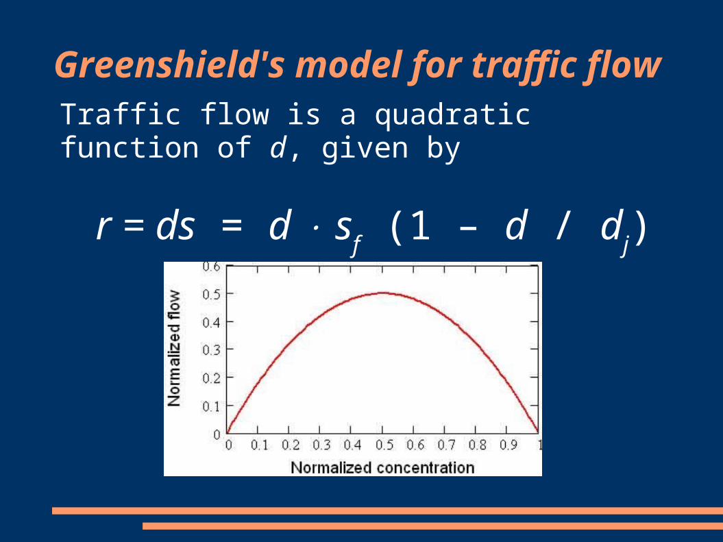
Greenshield's model for traffic flow
Traffic flow is a quadratic function of d, given by
r = ds = d sf (1 – d / d
j)
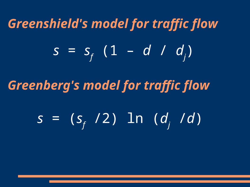
Greenshield's model for traffic flow
s = sf (1 – d / d
j)
Greenberg's model for traffic flow
s = (sf /2) ln (d
j /d)
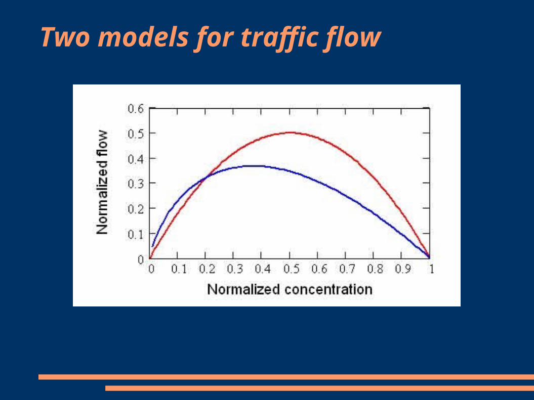
Two models for traffic flow

Mad cow disease
Annual deaths in the UK from vCJD (mad cow disease) from 1994 to 2006.
http://www.cjd.ed.ac.uk/vcjdqjun06.htm
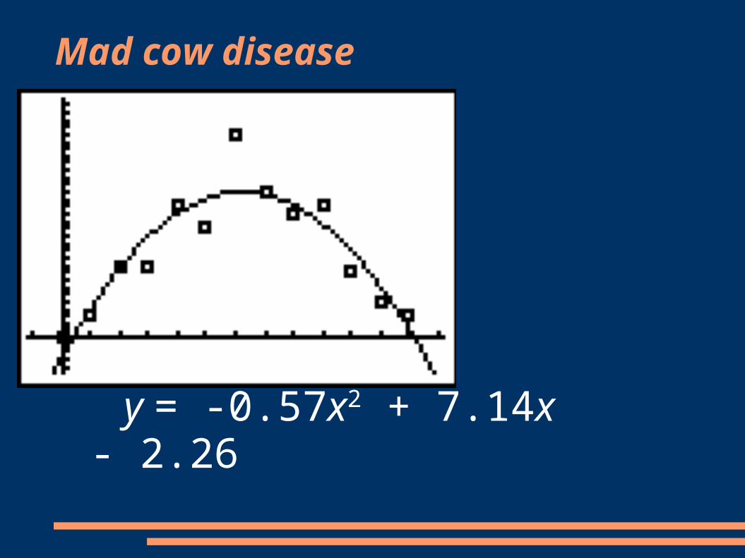
Mad cow disease
y = -0.57x2 + 7.14x - 2.26
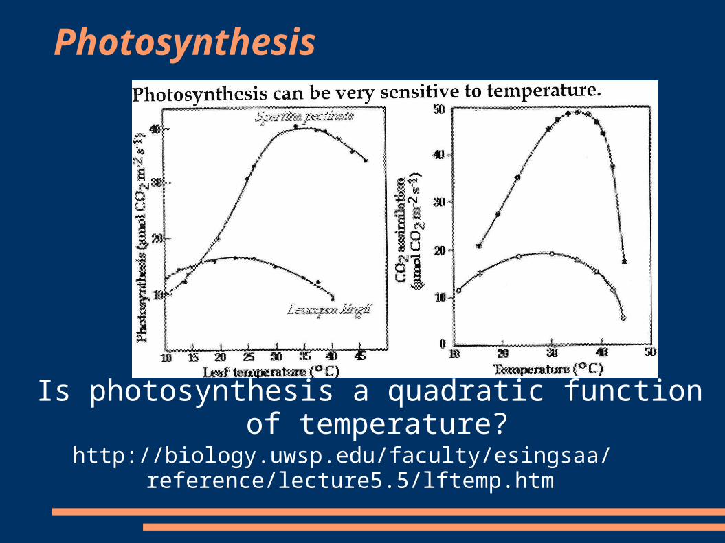
Photosynthesis
Is photosynthesis a quadratic function of temperature?
http://biology.uwsp.edu/faculty/esingsaa/reference/lecture5.5/lftemp.htm
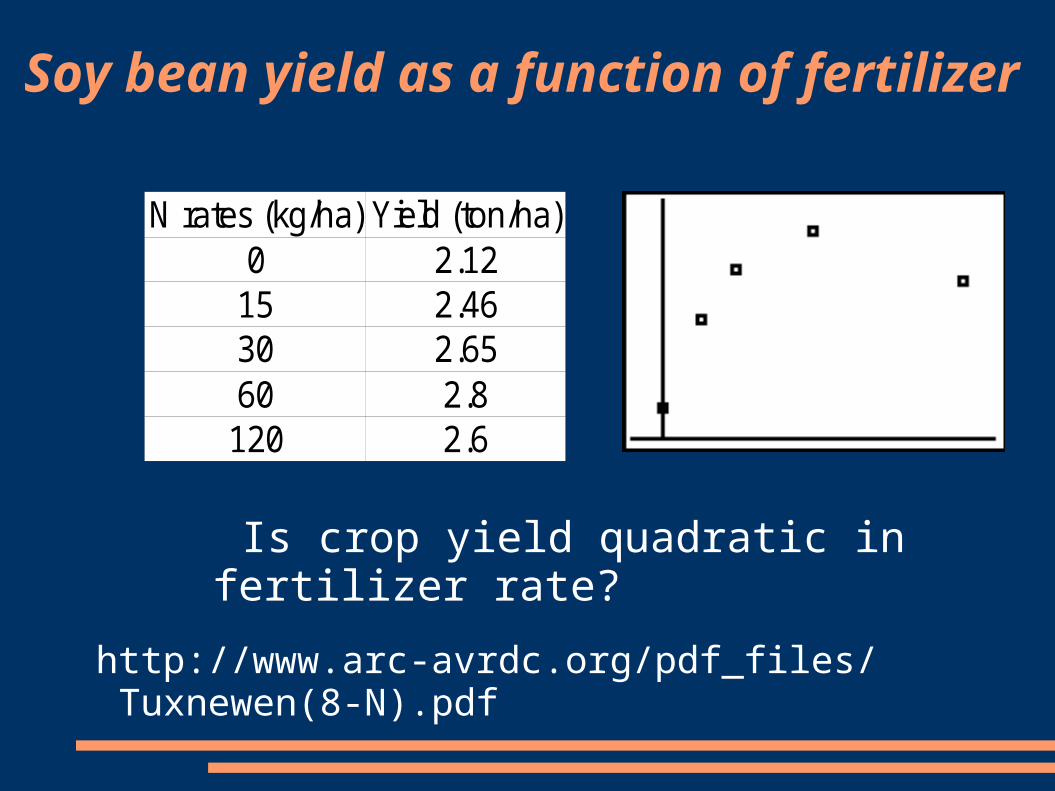
Soy bean yield as a function of fertilizer
Is crop yield quadratic in fertilizer rate?
N rates (kg/ha) Yield (ton/ha)0 2.12
15 2.4630 2.6560 2.8120 2.6
http://www.arc-avrdc.org/pdf_files/Tuxnewen(8-N).pdf
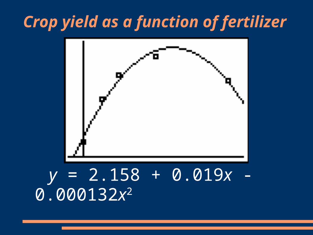
Crop yield as a function of fertilizer
y = 2.158 + 0.019x - 0.000132x2

But are these models or just examples of curve-fitting?
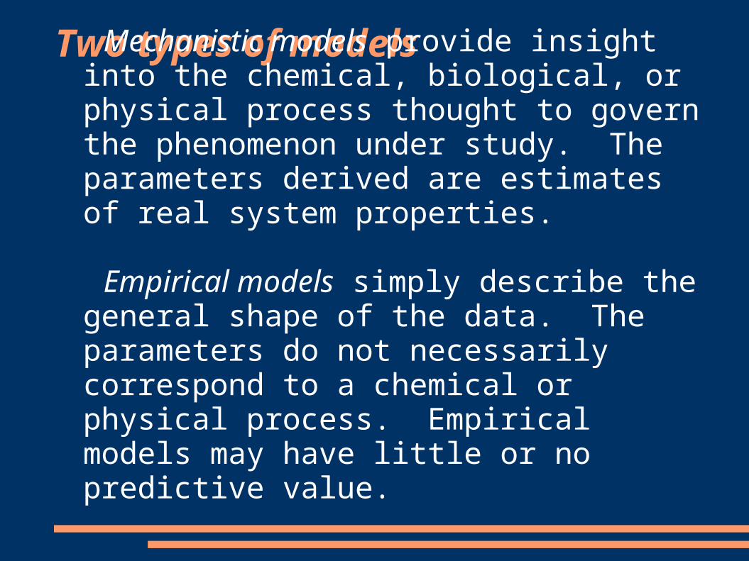
Two types of models Mechanistic models provide insight into the
chemical, biological, or physical process thought to govern the phenomenon under study. The parameters derived are estimates of real system properties.
Empirical models simply describe the general shape of the data. The parameters do not necessarily correspond to a chemical or physical process. Empirical models may have little or no predictive value.
Choosing a model: A quote from GraphPad Software
“Choosing a model is a scientific decision. You should base your choice on your understanding of chemistry or physiology (or genetics, etc.). The choice should not be based solely on the shape of the graph.”
“Some programs...automatically fit data to hundreds or thousands of equations and then present you with the equation(s) that fit the data best... You will not be able to interpret the best-fit values of the variables, and the results are unlikely to be useful for data analysis”
(Fitting Models to Biological Data Using Linear and Nonlinear Regression, Motulsky & Christopoulos, GraphPad Software, 2003)
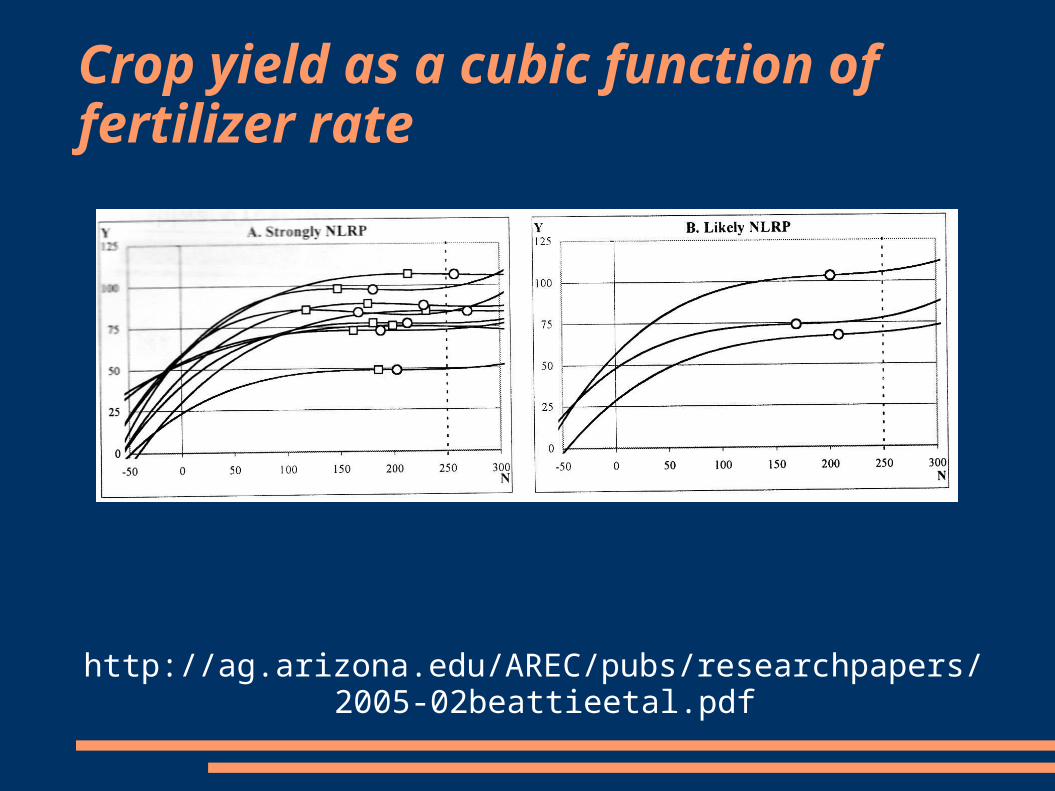
Crop yield as a cubic function of fertilizer rate
http://ag.arizona.edu/AREC/pubs/researchpapers/2005-02beattieetal.pdf

Cost function for higher education in Australia
http://www.melbourneinstitute.com

Visitor impact at tourist sites in New Zealand
http://www.landcareresearch.co.nz/research/sustain_business/tourism/documents/tourist_flow_data.pdf
Polynomial curve fitting
Although higher-degree polynomials typically do not provide meaningful models, they are useful for approximating continuous curves.
Polynomials are easy to evaluate, their graphs are completely smooth, and their derivatives and integrals are again polynomials.

Font design
Lagrange interpolation
Given any n + 1 points in the plane with distinct x-coordinates, there is a polynomial of degree at most n whose graph passes through those points.
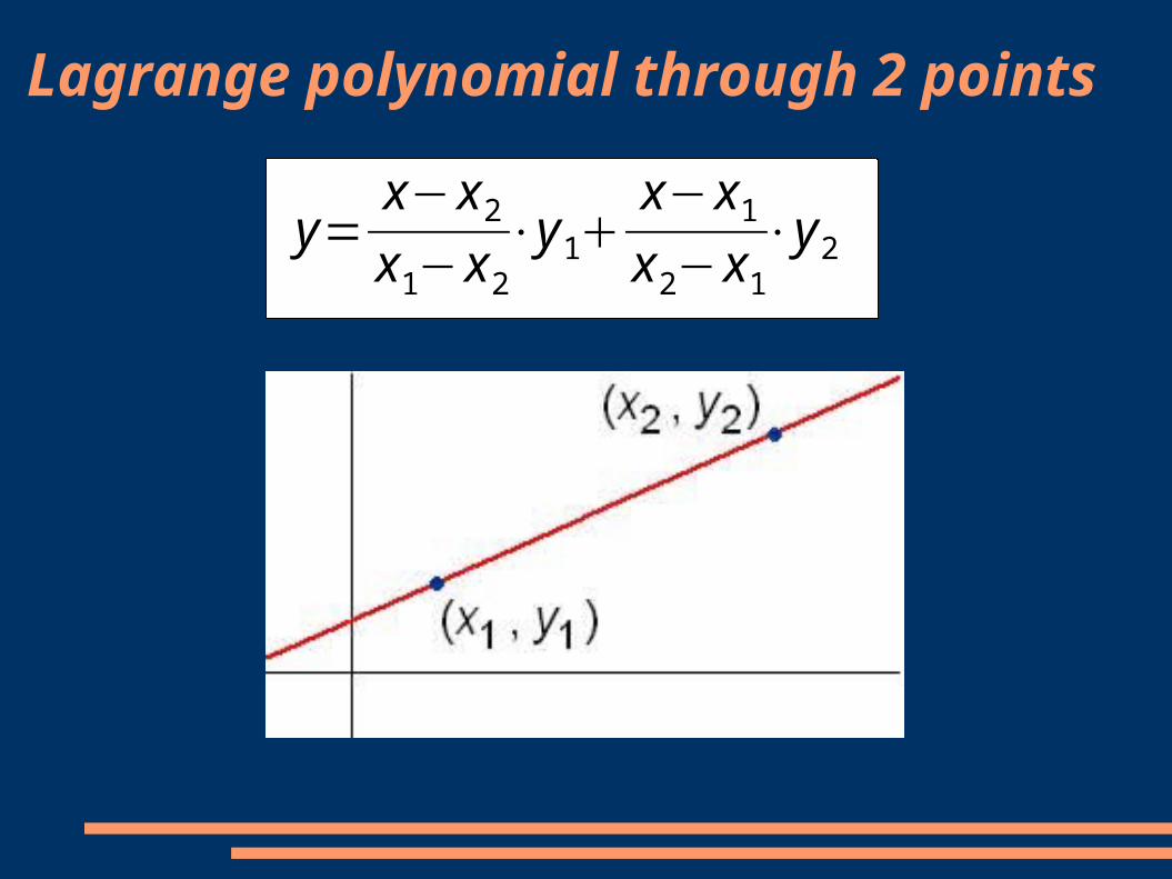
y=x−x2
x1−x2
⋅y1x−x1
x2−x1
⋅y2
Lagrange polynomial through 2 points
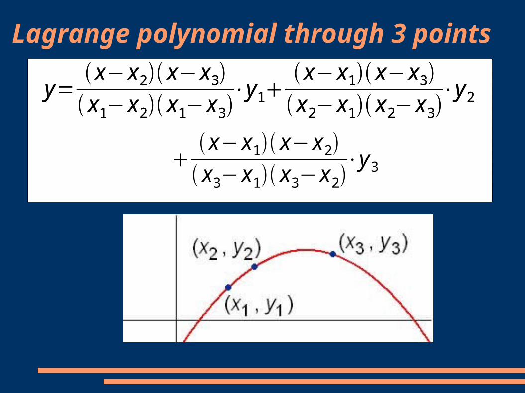
Lagrange polynomial through 3 points
y= x−x2 x−x3 x1−x2 x1−x3
⋅y1 x−x1 x−x3 x2−x1 x2−x3
⋅y2
x−x1 x−x2 x3−x1 x3−x2
⋅y3
y= x−x2 x−x3 x1−x2 x1−x3
⋅y1 x−x1 x−x3 x2−x1 x2−x3
⋅y2
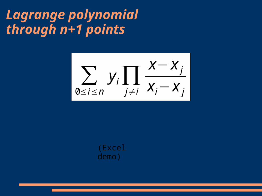
Lagrange polynomial through n+1 points
∑0≤i≤n
yi∏j≠i
x−x j
xi−x j
(Excel demo)
Osculating polynomials
An osculating polynomial agrees with the function and all its derivatives up to order m at n points in a given interval.
Hermite polynomials are osculating polynomials of order m = 1, that is, they agree with the function and its first derivative at each point.
Piecewise interpolation
Many of the most effective interpolation techniques use piecewise cubic Hermite polynomials.
There is a trade-off between smoothness and local monotonicity or shape-preservation.
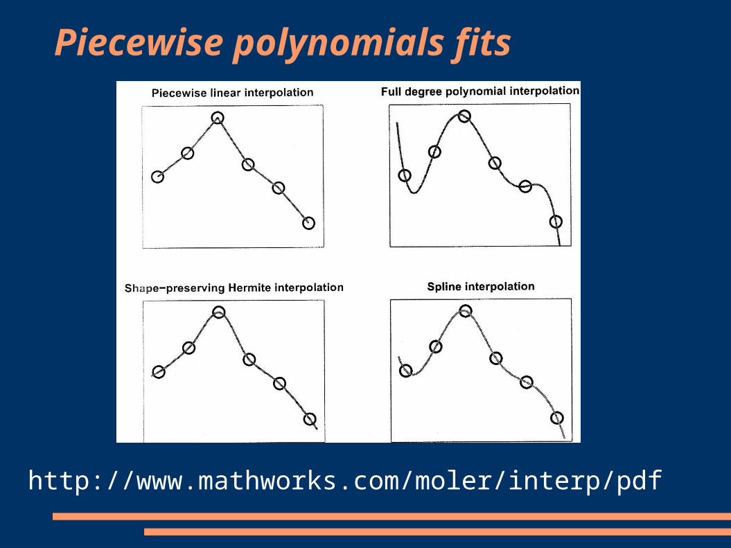
Piecewise polynomials fits
http://www.mathworks.com/moler/interp/pdf
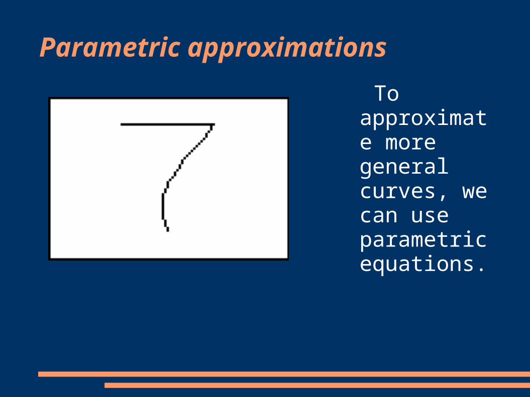
Parametric approximations
To approximate more general curves, we can use parametric equations.
Bezier curves
Bezier curves are the most frequently used interpolating curves in computer graphics.
They were developed in the 1960s by Paul de Casteljau, an engineer at Citroen, and independently by Pierre Bezier at Renault.
Linear Bezier curves
The linear Bezier curve through two points P0 and
P1 is defined by
P(t) = (1 – t) P0 + t P
1, 0 ≤ t ≤ 1
It is just the line segment joining P
0 and P
1.
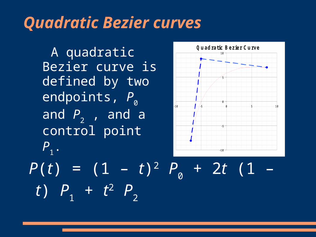
Quadratic Bezier curves
A quadratic Bezier curve is defined by two endpoints, P
0 and
P2 , and a control
point P1.
Qu adratic Bezier Cu rve
-10
-5
0
5
10
-10 -5 0 5 10
P(t) = (1 – t)2 P0 + 2t (1 – t) P
1 + t2 P
2
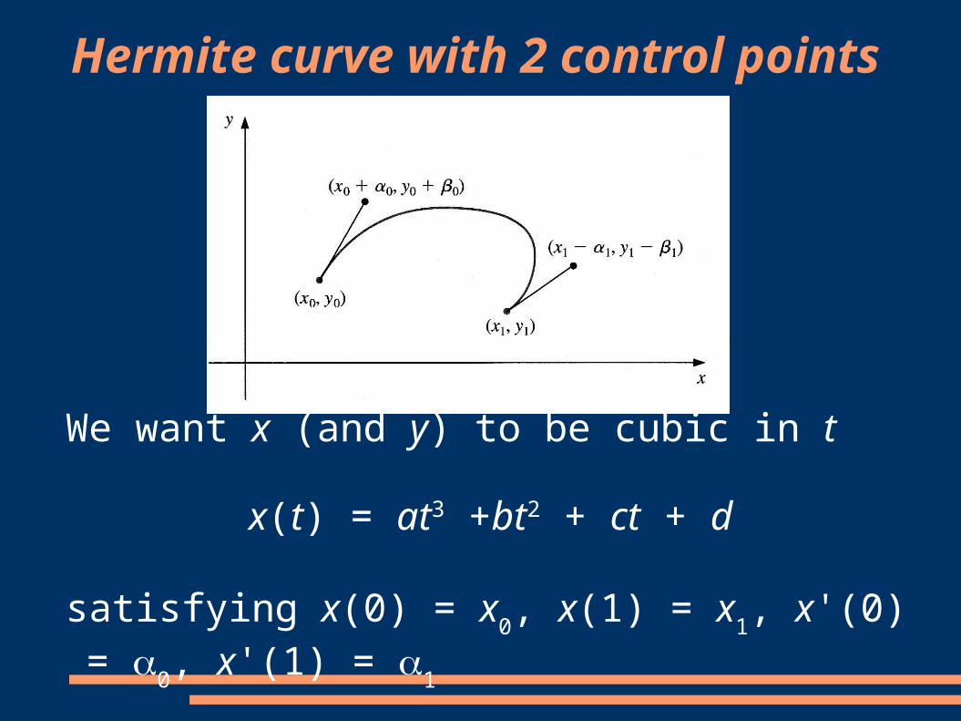
Hermite curve with 2 control points
We want x (and y) to be cubic in t
x(t) = at3 +bt2 + ct + d
satisfying x(0) = x0, x(1) = x
1, x'(0) =
0, x'(1) =
1
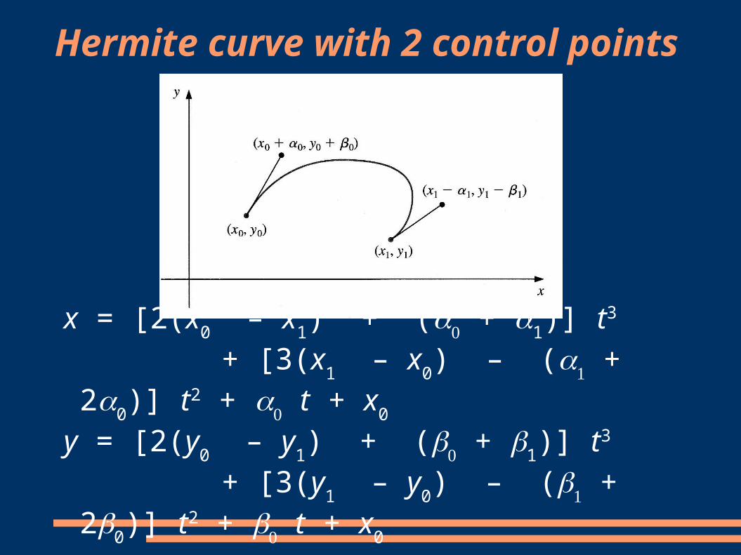
Hermite curve with 2 control points
x = [2(x0 – x
1) + ( +
1)] t3
+ [3(x1 – x
0) – ( + 2
0)] t2 + t + x
0
y = [2(y0 – y
1) + ( +
1)] t3
+ [3(y1 – y
0) – ( + 2
0)] t2 + t + x
0
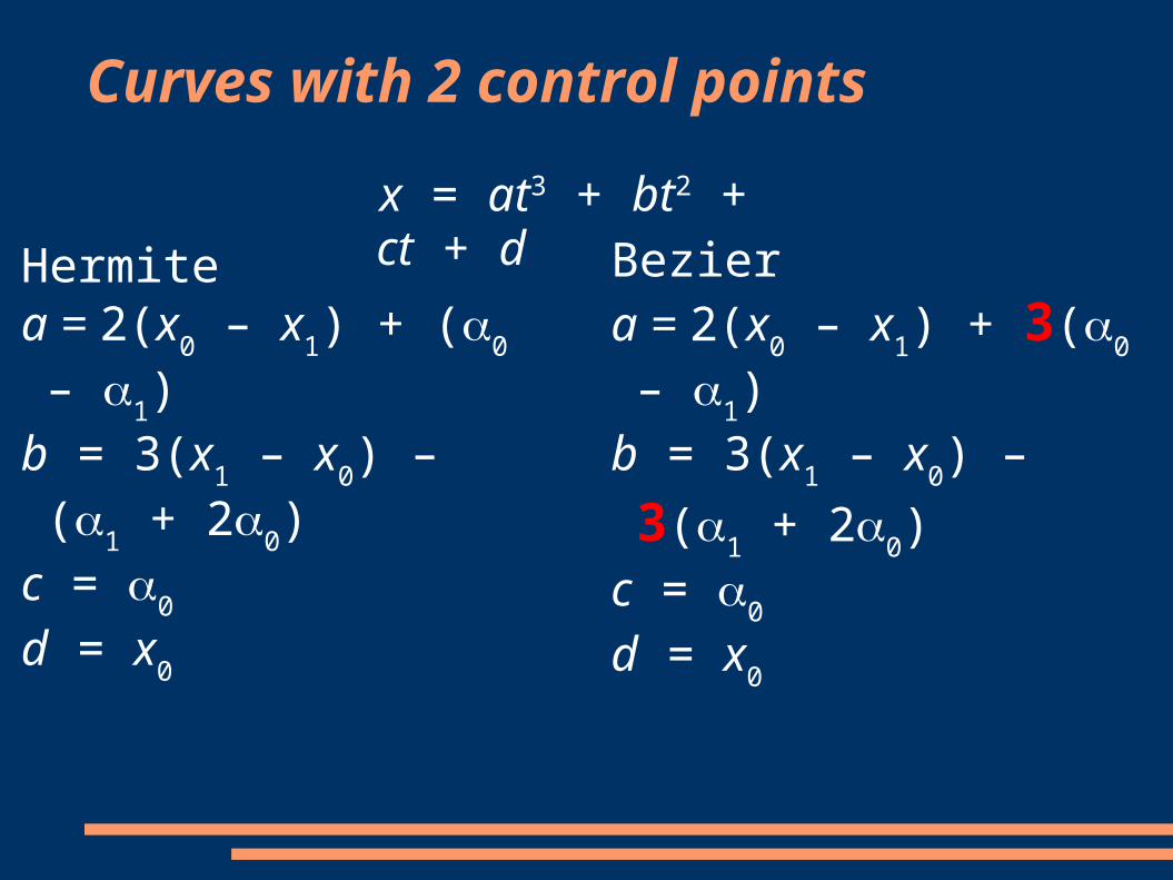
Curves with 2 control points
x = at3 + bt2 + ct + d
Beziera = 2(x
0 – x
1) + 3(
0 –
1)
b = 3(x1 – x
0) – 3(
1 + 2
0)
c = 0
d = x0
Hermitea = 2(x
0 – x
1) + (
0 –
1)
b = 3(x1 – x
0) – (
1 + 2
0)
c = 0
d = x0
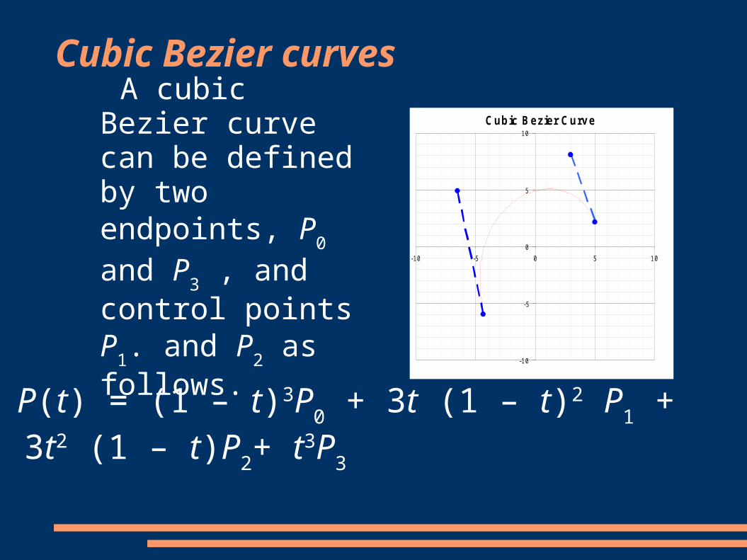
Cubic Bezier curves
A cubic Bezier curve can be defined by two endpoints, P
0 and P
3 ,
and control points P1.
and P2 as follows.
P(t) = (1 – t)3P0 + 3t (1 – t)2 P
1 + 3t2 (1 – t)P
2+ t3P
3
Cubic Bezier Curv e
-10
-5
0
5
10
-10 -5 0 5 10
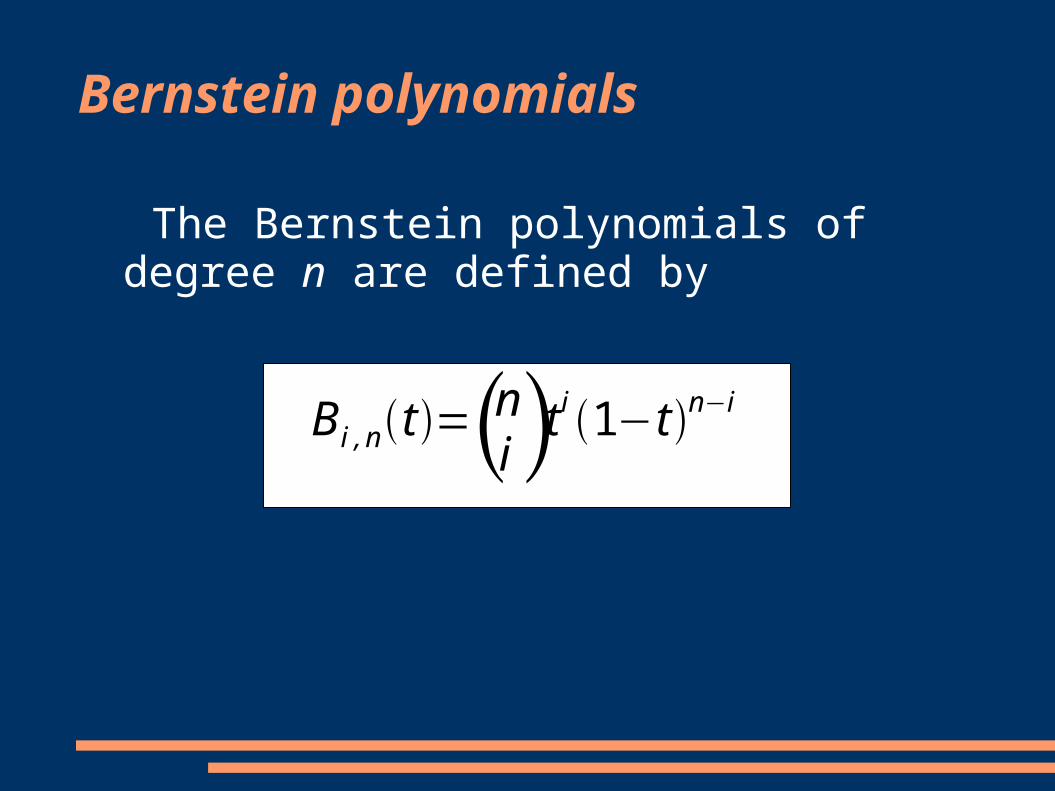
Bernstein polynomials
The Bernstein polynomials of degree n are defined by
Bi , n t =ni t i 1−t n−i
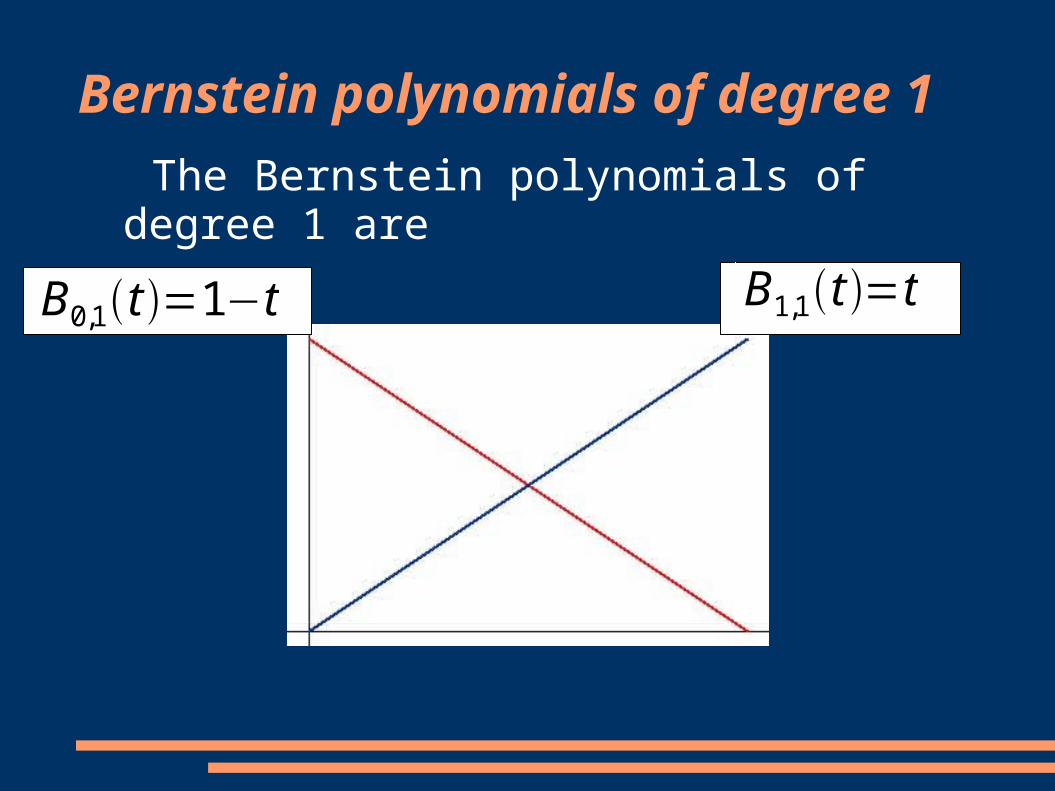
Bernstein polynomials of degree 1
The Bernstein polynomials of degree 1 are
B0,1 t =1−t B1,1 t =t
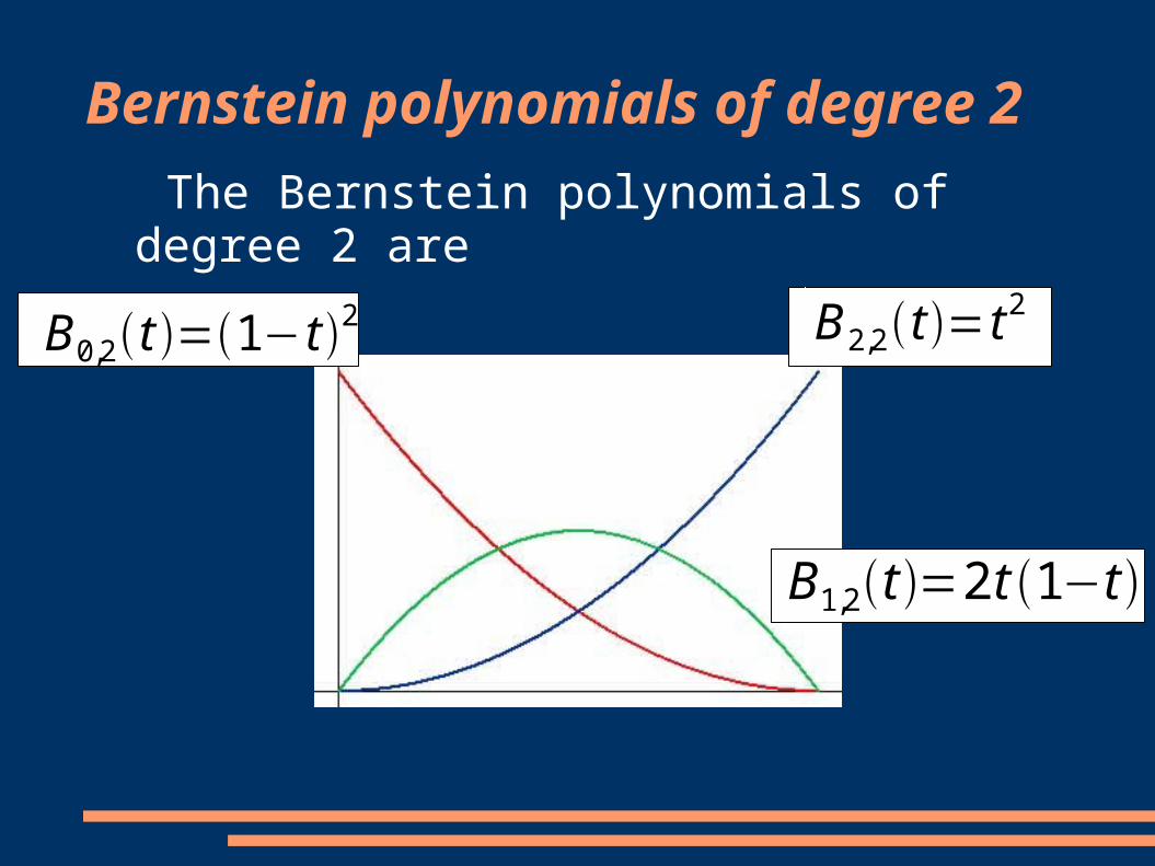
Bernstein polynomials of degree 2
The Bernstein polynomials of degree 2 are
B1,2 t =2 t 1−t
B2,2 t = t 2B0,2 t =1−t 2
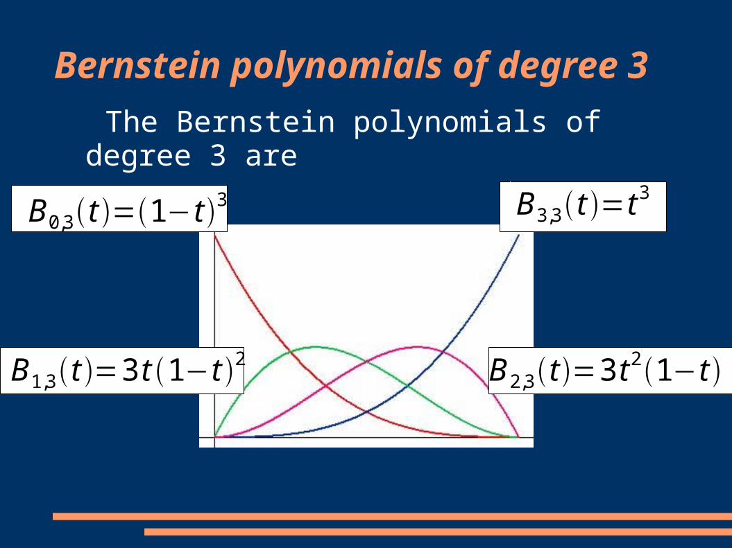
Bernstein polynomials of degree 3
The Bernstein polynomials of degree 3 are
B1,3 t =3 t 1−t 2 B2,3 t =3 t 2 1−t
B3,3 t =t 3B0,3 t =1−t 3
Bernstein polynomials
● Form a basis for polynomials of degree n.● Form a partition of unity, that is, the sum of
the Bernstein polynomials of degree n is 1.● When a Bezier polynomial is expressed in
terms of the Bernstein basis, the coefficients of the basis elements are just the points P
0
through Pn.

Download presentation and handouts
www.piercecollege.edu/faculty/yoshibw/Talks/
amatyc06/