Curves

First of all…

• You may ask yourselves “What did those papers have to do with computer graphics?”– Valid question

• Answer: I thought they were cool, unique applications of computer graphics

• This week we’re looking at scan conversion of curves

Interpolation

• Bresenham’s line drawing algorithm is nothing more than a form of interpolation– Given two points, find the location of points

in between them– The function (in this case it’s a line) must

pass through the given points, by definition

Interpolation Usage

• We used Bresenham line drawing (interpolation) to scan convert a symbolic representation of a line to a rasterized line

• Other applications exist– Computing calendar years are leap years (believe

it or not)• Line Drawing, Leap Years, and Euclid, Harris and

Reingold, ACM Computing Surveys, Vol. 36, No. 1, March 2004, pp. 66-80

– Path planning for key frame animation

Key Frame Animation

• Key frames are infrequent scenes that capture the essential flow of an animation– Think of them as the endpoints of a line

• In between frames (tweens) may be generated by interpolating between two key frames– Think of these as the points drawn by the

Bresenham algorithm

Approximation

• Another possibility for generating tweens is to specify tie-points that guide the generation of the intermediate path points but the path does not pass through the tie-points

• This technique is called approximation or curve fitting

Curves

• We’ll look at two techniques for generating curves (to be used as either paths or drawn objects)– Interpolation– Approximation

• We’ll also see that interpolation is very restrictive when considering parametric curves

• Approximation is a much better approach

Parametric Curves

• Recall the parametric line equations

• The parameter t is used to map out a set of (x, y) pairs that represent the line

10

010

010

t

tyyyytxxxx

Parametric Curves

• In the case of a curve the parametric function is of the form– Q(u) = (x(u), y(u), z(u)) in 3 dimensions

• The derivative of Q(u) is of the form– Q’(u) = (x’(u), y’(u), z’(u))

• Significance of the derivative?– It is the tangent vector at a given point (u) on

the curve

Derivative

Parametric Curves

• In the case of object drawing, u is a spatial parameter (like t was for the line)

• In the case of key frame animation, u is a temporal parameter

• In both cases Q(0) is the start of the curve and Q(1) is the end, as was the case for the parametric line

Parametric Curves

• Curvature

• Curvature k = 1/ ρ• The higher the curvature, the more the curve

bends at the given point

Osculating circle of radius ρ touches the curve at exactly 1 point

ρ

Parametric Curves

• From calculus, a function f is continuous at a value x0 if

• In layman’s terms this means that we can draw the curve without ever lifting our pen from the drawing surface

• f(x) is continuous over an interval (a,b) if it is continuous for every point in the interval

• We call this C0 continuity

)()(lim0

0xx ff

xx

Parametric Curves

a

b

ab

Continuous over (a,b) – C0

Continuous over (a,b) – C0

Parametric Curves

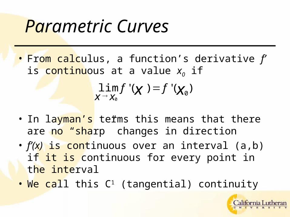
• From calculus, a function’s derivative f’ is continuous at a value x0 if

• In layman’s terms this means that there are no “sharp” changes in direction

• f’(x) is continuous over an interval (a,b) if it is continuous for every point in the interval

• We call this C1 (tangential) continuity

)(')('lim0

0

xx ffxx

Parametric Curves

a

b

ab

Continuous derivative over (a,b) – C1

Discontinuous derivative over (a,b) – not C1

Parametric Curves

• When we need to join two curves at a single point we can guarantee C1 continuity across the joint– For the case when we can’t make one continuous

curve– Just make sure that the tangents of the two curves at

the join are of equal length and direction

• If the tangents at the joint are of identical direction but differing lengths (change in curvature) then we have G1 continuity

Lagrange Polynomials

• To generate a function that passes through every specified point, the type of function depends on the number of specified points– Two points → linear function– Three points → quadratic function– Four points → cubic function

• Generating such functions makes use of Lagrange polynomials

Lagrange Polynomials

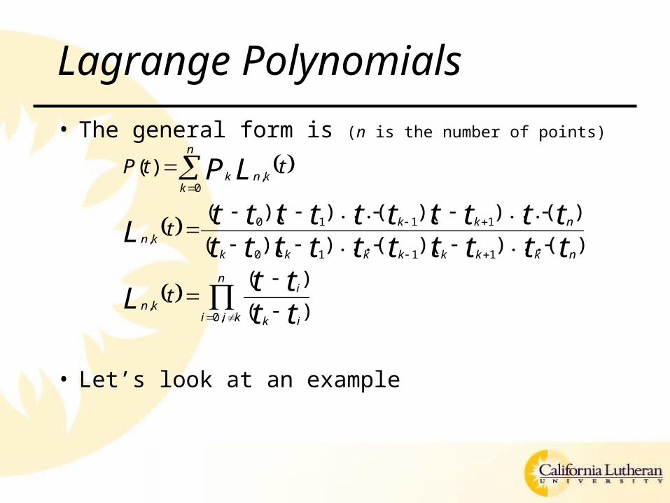
• The general form is (n is the number of points)

• Let’s look at an example

n

kii ik

i

kn

nkkkkkkk

nkk

kn

n

kknk

tttt

L

tttttttttttttttttttt

L

LP

t

t

ttP

,0,

1110

1110

,

0,

)(

)(

))...()()...()((

))...()()...()((

)(

Lagrange Polynomials

• For two points P0 and P1:

• For the starting point (t0=0) and ending point (t1=1)

Ptt

ttPtt

tttP

101

0

010

1)(

PP

Pt

Pt

tttP

tP

10

10

)()1()(

01

0

10

1)(

Lagrange Polynomials

• For three points P0 , P1 , and P2:

• And it only gets worse for larger numbers of points• Suffice it to say, this isn’t the most optimum way to

draw curves– Too many operations per point

– Too complex if the artist decides to change the curve

– But you could do it

Ptttt

ttttPtttt

ttttPtttt

tttttP

22202

10

12101

20

02010

21)(

A Better Way

• The problem with Lagrange polynomials lies in the fact that we try to make the curve pass through all of the specified points

• A better way is to specify points that control how the curve passes from one point to the next

• We do so by specifying a cubic function controlled by four points

• The four points are called boundary conditions

Hermite Boundary Conditions

• Two points• Two tangent vectors

– Two of the points are interpreted as vectors off of the other two points

P0 P1

P’1P’0

Cubic Functions

• Generalized form

• Derivative

• Our goal is to “solve” these equations in “closed form” so that we can generate a series of points on the curve

DucubuauQ 23)(

cubuauQ 232

)('

This is why it’s called a “cubic” function

Cubic Functions

• There are four unknown values in the equation– a, b, c, and D (remember, a, b, c, and D are vectors in x, y, z

so there is actually a set of 3 equations)

• We need to use these equations to generate values of x, y, and z along the curve

• We can generate a closed form solution (solve the equations for x, y, and z) since we have four known boundary conditions

u = 0 → Q(0) = P0 and Q’(0) = P’0

u = 1 → Q(1) = P1 and Q’(1) = P’1

Solution of Equations

• Go to the white board…

Implementation• So, all you have to do to generate a curve is to implement this vector (x, y,

z) equation:

by stepping 0 ≤ u ≤ 1

• P0, P1, P0’ and P1

’ are vectors in x, y, z so there are really 12 coefficients to be computed and you’ll be implementing 3 equations for Q(u)

0

'0

'1

'010

'1

'010

23

233

22

)(

PD

Pc

PPPPb

PPPPa

where

DcubuauuQ

)(),(),( uQuQuQ zyx

Implementation

• Note that you’ll have to estimate the step size for u or…(any ideas?)

• …use your Bresenham code to draw short straight lines between the points you generate on the curve (to fill gaps)

• There is no trick (that I’m aware of) comparable to the Bresenham approach

Bezier Curves

• Similar derivation to Hermite

• Different boundary conditions– Bezier uses 2 endpoints and 2 control

points (rather than 2 endpoints and 2 slopes)

Bezier Curves

EndpointsControl points

Implementation• So, all you have to do to generate a curve is to implement this vector (x, y,

z) equation:

by stepping 0 ≤ u ≤ 1

• P0, P1, P2 and P3 are vectors in x, y, z so there are really 12 coefficients to be computed and you’ll be implementing 3 equations for Q(u)

0

10

210

3210

23

33

363

33

)(

PD

PPc

PPPb

PPPPa

where

DcubuauuQ

)(),(),( uQuQuQ zyx

Bezier example

Hermite vs. Bezier

• Hermite is easy to control continuity at the endpoints when joining multiple curves to create a path– But difficult to control the “internal” shape of the curve

• Bezier is easy to control the “internal” shape of the curve– But a little more (not much) difficult to control continuity at

the endpoints when joining multiple curves to create a path

• Bottom line is, when creating a path you have to be very selective about endpoints and adjacent control points (Bezier) or tangent slopes (Hermite)

Result

• Go to the demo program…

• My code generates a Hermite curve that is of C1 continuity– As I generate new segments along the

curve I join them by keeping the adjoining tangent vectors equal

Homework

• Implement Bezier and Hermite curve drawing– Parameters should be control points and brush width

• Create a video sequence to show in class– Demonstrate Bezier and Hermite curves of various control

points and brush widths– Be creative

• Due date – Next week – Turn in:– Video to be shown in class– All program listings

• Grading will be on completeness (following instructions) and timeliness (late projects will be docked 10% per week)