customer profitability analysis, sales performance ... · customer profitability analysis, sales...
TRANSCRIPT
©McGraw-Hill Ryerson Limited, 2001Irwin/McGraw-Hill Ryerson
18-1
Customer Profitability Analysis,Sales Performance Evaluation,
and Income Reporting
Student Tutorial
18
©McGraw-Hill Ryerson Limited, 2001Irwin/McGraw-Hill Ryerson
18-2
Chapter Organization
This chapter has been subdivided into threeindependent sections.
Click the section below that you wish to study,or press “Enter” to proceed linearly through
the chapter.!Customer Profitability Analysis"Sales Variance Analysis#Income Reporting Effects of Alternative
Product-Costing Approaches
©McGraw-Hill Ryerson Limited, 2001Irwin/McGraw-Hill Ryerson
18-3
Customer Profitability Analysis
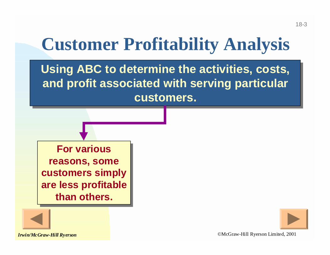
Using ABC to determine the activities, costs,and profit associated with serving particular
customers.
Using ABC to determine the activities, costs,and profit associated with serving particular
customers.
For variousreasons, some
customers simplyare less profitable
than others.
For variousreasons, some
customers simplyare less profitable
than others.
©McGraw-Hill Ryerson Limited, 2001Irwin/McGraw-Hill Ryerson
18-4
Customer Profitability Analysis
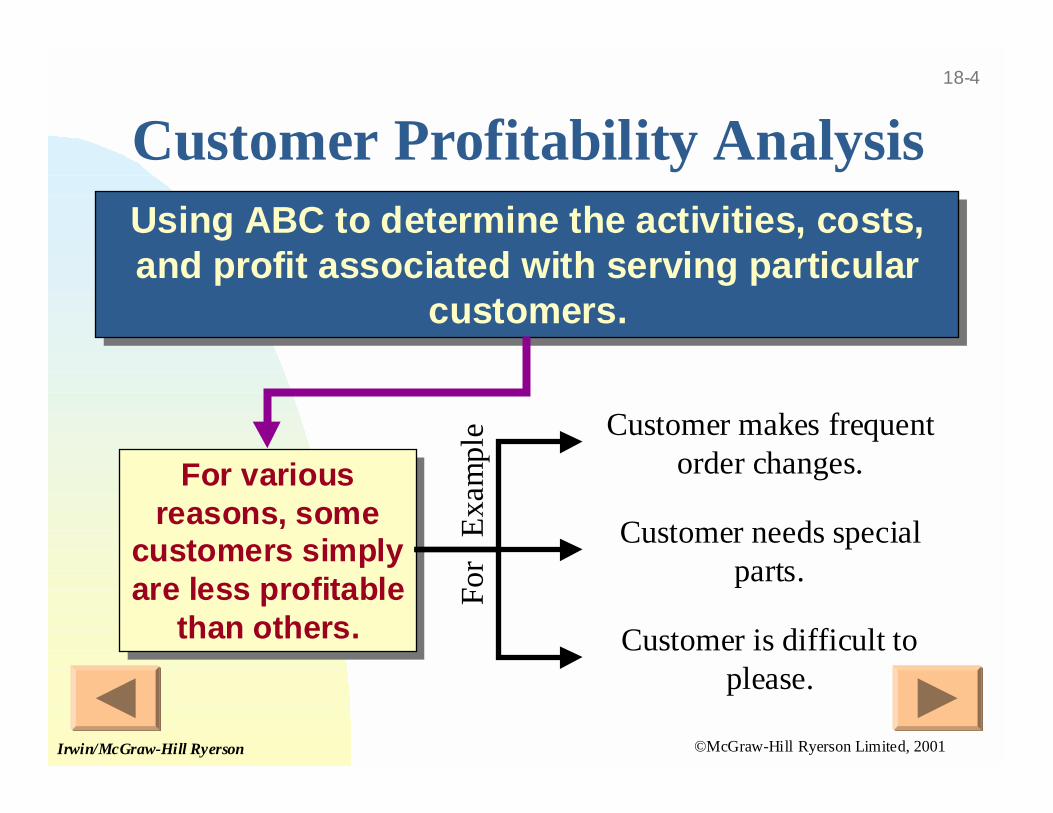
Using ABC to determine the activities, costs,and profit associated with serving particular
customers.
Using ABC to determine the activities, costs,and profit associated with serving particular
customers.
For variousreasons, some
customers simplyare less profitable
than others.
For variousreasons, some
customers simplyare less profitable
than others.
Customer makes frequentorder changes.
Customer needs specialparts.
Customer is difficult toplease.
For
Exa
mpl
e
©McGraw-Hill Ryerson Limited, 2001Irwin/McGraw-Hill Ryerson
18-5
Customer Profitability Analysis
Once we know which customers are the leastprofitable, we can modify our relationship to
improve profitability.
Once we know which customers are the leastprofitable, we can modify our relationship to
improve profitability.
I hate to do this, but we
just can’t continue doing
business with you.
Examples:Examples:
©McGraw-Hill Ryerson Limited, 2001Irwin/McGraw-Hill Ryerson
18-6
Customer Profitability Analysis
Once we know which customers are the leastprofitable, we can modify our relationship to
improve profitability.
Once we know which customers are the leastprofitable, we can modify our relationship to
improve profitability.
We’ll send a team to your plantnext week and help you set up an
ordering system that gives usmore lead time.
Examples:Examples:
©McGraw-Hill Ryerson Limited, 2001Irwin/McGraw-Hill Ryerson
18-7
Customer Profitability Analysis
Once we know which customers are the leastprofitable, we can modify our relationship to
improve profitability.
Once we know which customers are the leastprofitable, we can modify our relationship to
improve profitability.
If you ask forfewer changes,we can charge
you less!
Examples:Examples:
©McGraw-Hill Ryerson Limited, 2001Irwin/McGraw-Hill Ryerson
18-8
Customer Profitability Analysis
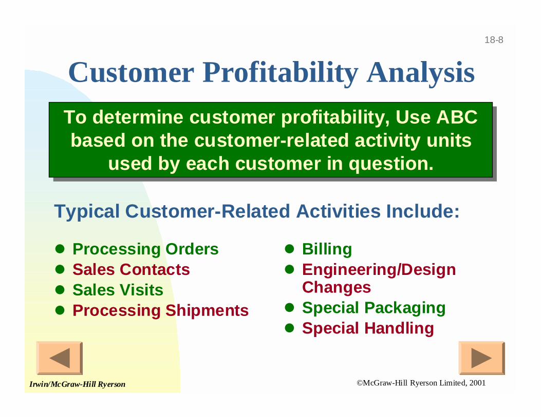
$ Processing Orders$ Sales Contacts$ Sales Visits$ Processing Shipments
To determine customer profitability, Use ABCbased on the customer-related activity units
used by each customer in question.
To determine customer profitability, Use ABCbased on the customer-related activity units
used by each customer in question.
Typical Customer-Related Activities Include:
$ Billing$ Engineering/Design
Changes$ Special Packaging$ Special Handling
©McGraw-Hill Ryerson Limited, 2001Irwin/McGraw-Hill Ryerson
18-9
Customer Profitability AnalysisExample
-$100,000
-$50,000
$0
$50,000
$100,000
$150,000
$200,000
107 108 101 102 114
Cus
tom
er P
rofi
tabi
lity
Customer #
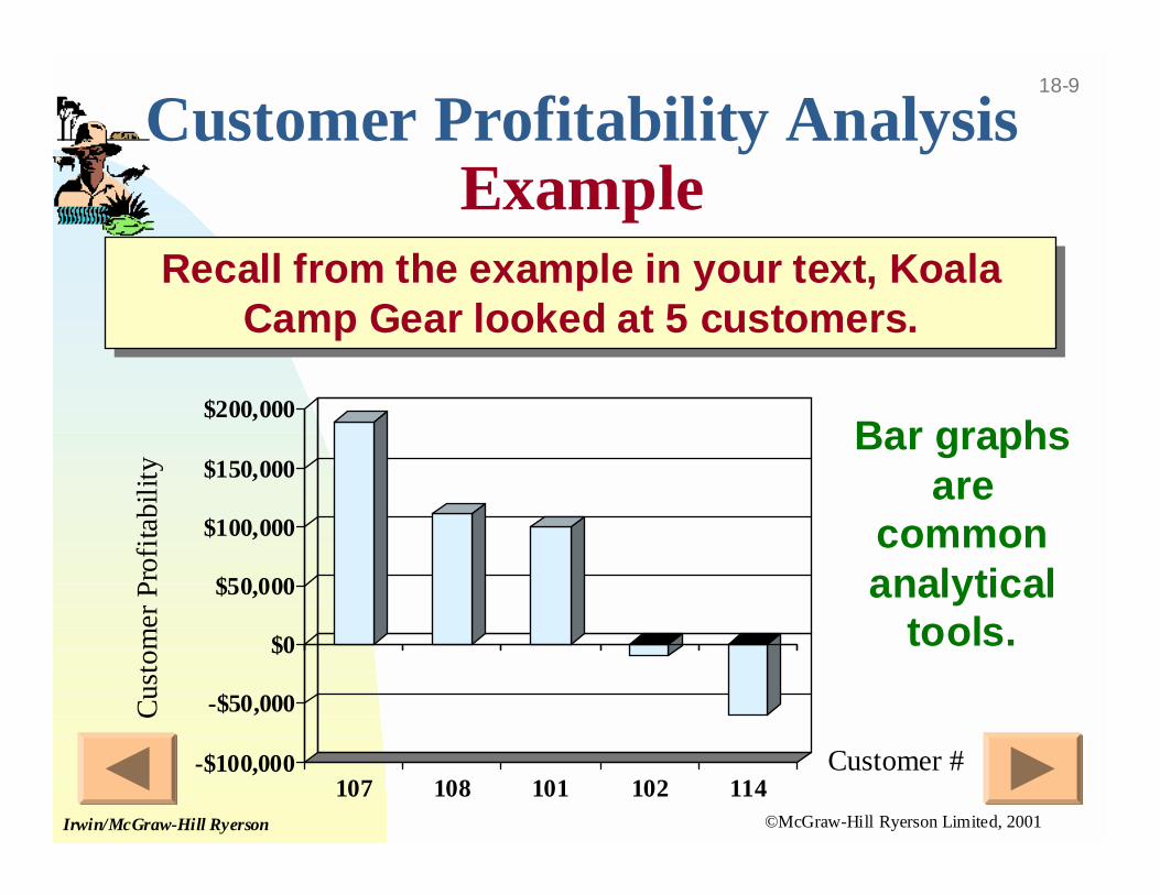
Recall from the example in your text, KoalaCamp Gear looked at 5 customers.
Recall from the example in your text, KoalaCamp Gear looked at 5 customers.
Bar graphsare
commonanalytical
tools.
©McGraw-Hill Ryerson Limited, 2001Irwin/McGraw-Hill Ryerson
18-10
Customer #
Customer Profitability AnalysisExample
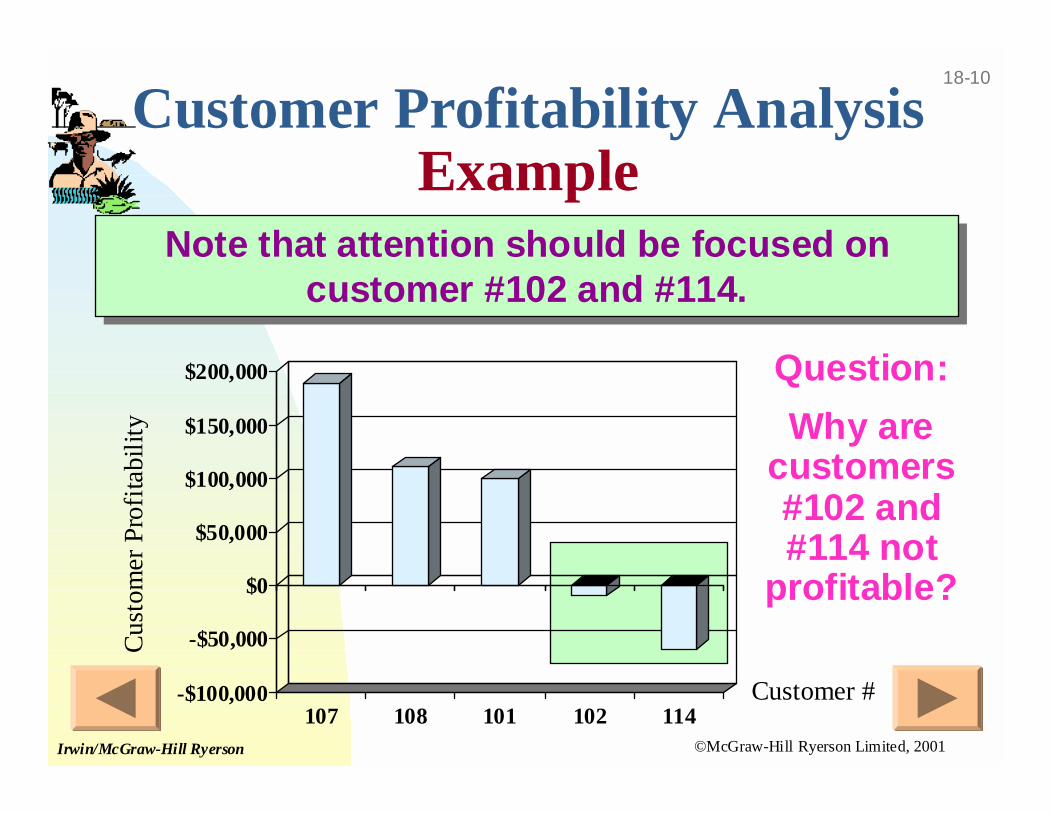
Note that attention should be focused oncustomer #102 and #114.
Note that attention should be focused oncustomer #102 and #114.
Question:
Why arecustomers#102 and#114 not
profitable?
-$100,000
-$50,000
$0
$50,000
$100,000
$150,000
$200,000
107 108 101 102 114
Cus
tom
er P
rofi
tabi
lity
©McGraw-Hill Ryerson Limited, 2001Irwin/McGraw-Hill Ryerson
18-11
Customer Profitability AnalysisExample
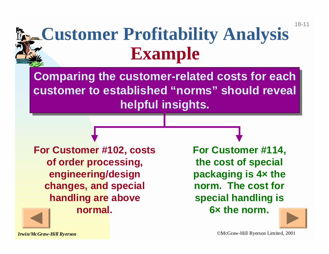
Comparing the customer-related costs for eachcustomer to established “norms” should reveal
helpful insights.
Comparing the customer-related costs for eachcustomer to established “norms” should reveal
helpful insights.
For Customer #102, costsof order processing,engineering/design
changes, and specialhandling are above
normal.
For Customer #114,the cost of specialpackaging is 4× thenorm. The cost forspecial handling is
6× the norm.
©McGraw-Hill Ryerson Limited, 2001Irwin/McGraw-Hill Ryerson
18-12
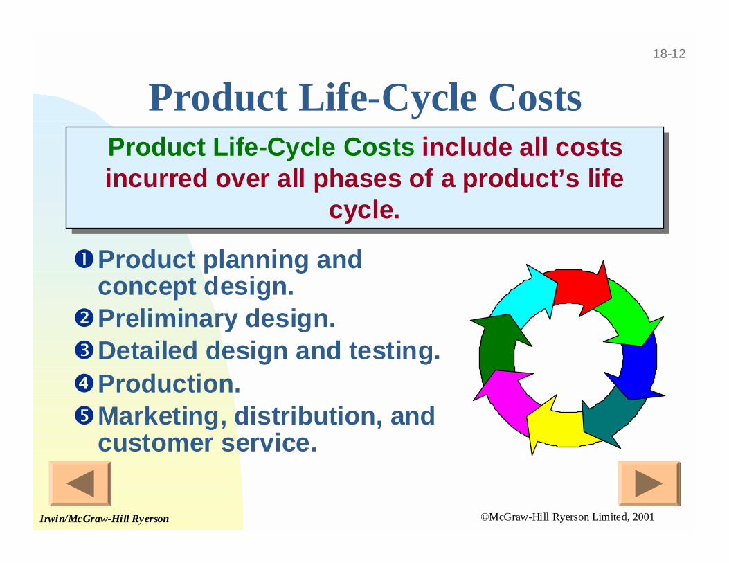
Product Life-Cycle CostsProduct Life-Cycle Costs include all costsincurred over all phases of a product’s life
cycle.
Product Life-Cycle Costs include all costsincurred over all phases of a product’s life
cycle.
!Product planning andconcept design.
"Preliminary design.#Detailed design and testing.%Production.&Marketing, distribution, and
customer service.
©McGraw-Hill Ryerson Limited, 2001Irwin/McGraw-Hill Ryerson
18-13
Let’s Lookat Sales
Variances.
©McGraw-Hill Ryerson Limited, 2001Irwin/McGraw-Hill Ryerson
18-14
Sales Variance Analysis
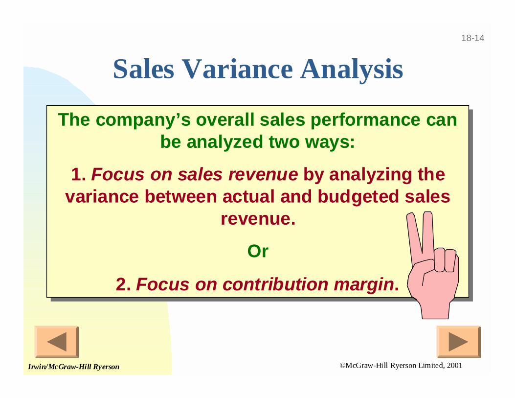
The company’s overall sales performance canbe analyzed two ways:
1. Focus on sales revenue by analyzing thevariance between actual and budgeted sales
revenue.
Or
2. Focus on contribution margin.
The company’s overall sales performance canbe analyzed two ways:
1. Focus on sales revenue by analyzing thevariance between actual and budgeted sales
revenue.
Or
2. Focus on contribution margin.
©McGraw-Hill Ryerson Limited, 2001Irwin/McGraw-Hill Ryerson
18-15
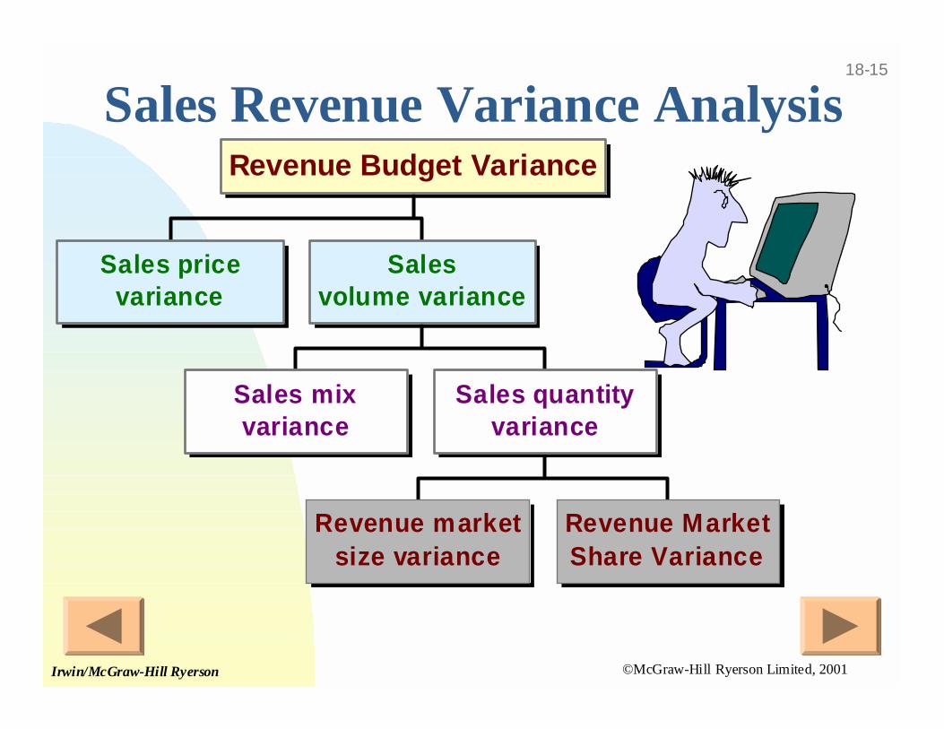
Sales Revenue Variance Analysis
Sales pricevariance
Sales mixvariance
Revenue marketsize variance
Revenue MarketShare Variance
Sales quantityvariance
Salesvolume variance
Revenue Budget Variance
©McGraw-Hill Ryerson Limited, 2001Irwin/McGraw-Hill Ryerson
18-16
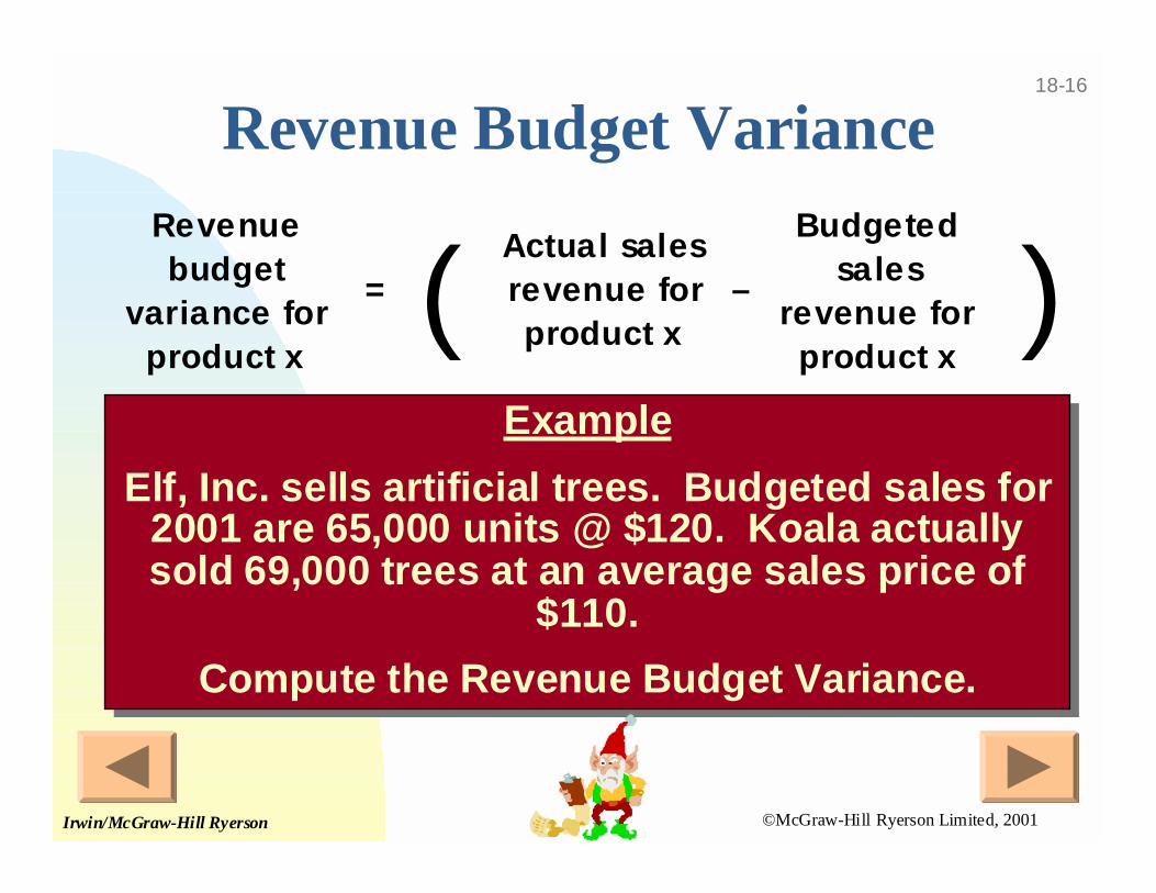
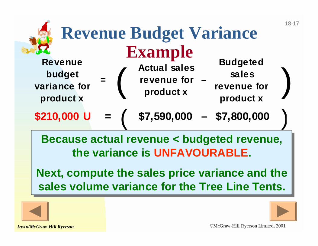
Revenue Budget VarianceRevenue budget
variance for product x
= (Actual sales revenue for product x
–
Budgeted sales
revenue for product x
)Example
Elf, Inc. sells artificial trees. Budgeted sales for2001 are 65,000 units @ $120. Koala actuallysold 69,000 trees at an average sales price of
$110.
Compute the Revenue Budget Variance.
Example
Elf, Inc. sells artificial trees. Budgeted sales for2001 are 65,000 units @ $120. Koala actuallysold 69,000 trees at an average sales price of
$110.
Compute the Revenue Budget Variance.
©McGraw-Hill Ryerson Limited, 2001Irwin/McGraw-Hill Ryerson
18-17
Revenue Budget VarianceExample
$210,000 U = ( $7,590,000 – $7,800,000 )Because actual revenue < budgeted revenue,
the variance is UNFAVOURABLE.
Next, compute the sales price variance and thesales volume variance for the Tree Line Tents.
Because actual revenue < budgeted revenue,the variance is UNFAVOURABLE.
Next, compute the sales price variance and thesales volume variance for the Tree Line Tents.
Revenue budget
variance for product x
= (Actual sales revenue for product x
–
Budgeted sales
revenue for product x
)
©McGraw-Hill Ryerson Limited, 2001Irwin/McGraw-Hill Ryerson
18-18
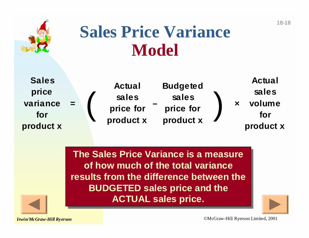
Sales Price VarianceModel
Sales price
variance for
product x
= (Actual sales
price for product x
–
Budgeted sales
price for product x
) ×
Actual sales
volume for
product x
The Sales Price Variance is a measureof how much of the total variance
results from the difference between theBUDGETED sales price and the
ACTUAL sales price.
The Sales Price Variance is a measureof how much of the total variance
results from the difference between theBUDGETED sales price and the
ACTUAL sales price.
©McGraw-Hill Ryerson Limited, 2001Irwin/McGraw-Hill Ryerson
18-19
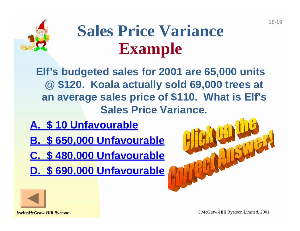
Sales Price VarianceExample
Elf’s budgeted sales for 2001 are 65,000 units@ $120. Koala actually sold 69,000 trees at
an average sales price of $110. What is Elf’sSales Price Variance.
A. $ 10 Unfavourable
B. $ 650,000 Unfavourable
C. $ 480,000 Unfavourable
D. $ 690,000 Unfavourable
©McGraw-Hill Ryerson Limited, 2001Irwin/McGraw-Hill Ryerson
18-20
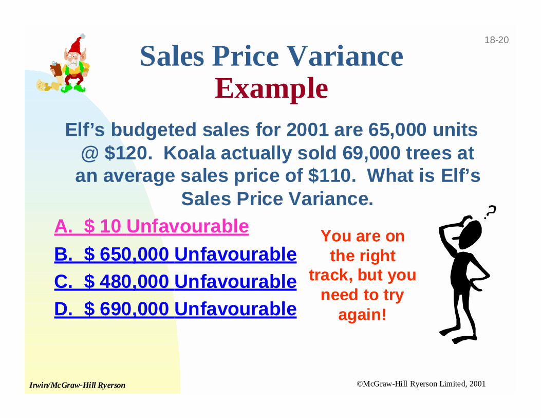
Sales Price VarianceExample
Elf’s budgeted sales for 2001 are 65,000 units@ $120. Koala actually sold 69,000 trees at
an average sales price of $110. What is Elf’sSales Price Variance.
A. $ 10 Unfavourable
B. $ 650,000 Unfavourable
C. $ 480,000 Unfavourable
D. $ 690,000 Unfavourable
You are onthe right
track, but youneed to try
again!
©McGraw-Hill Ryerson Limited, 2001Irwin/McGraw-Hill Ryerson
18-21
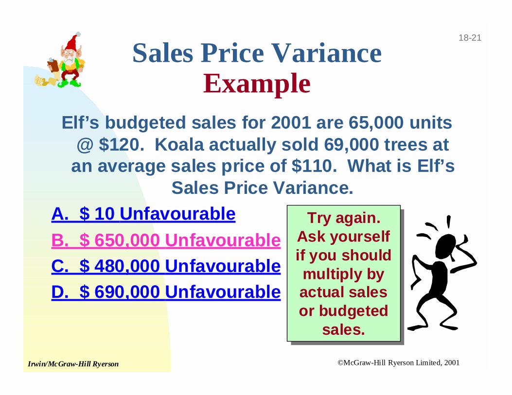
Sales Price VarianceExample
Elf’s budgeted sales for 2001 are 65,000 units@ $120. Koala actually sold 69,000 trees at
an average sales price of $110. What is Elf’sSales Price Variance.
A. $ 10 Unfavourable
B. $ 650,000 Unfavourable
C. $ 480,000 Unfavourable
D. $ 690,000 Unfavourable
Try again.Ask yourselfif you shouldmultiply byactual salesor budgeted
sales.
Try again.Ask yourselfif you shouldmultiply byactual salesor budgeted
sales.
©McGraw-Hill Ryerson Limited, 2001Irwin/McGraw-Hill Ryerson
18-22
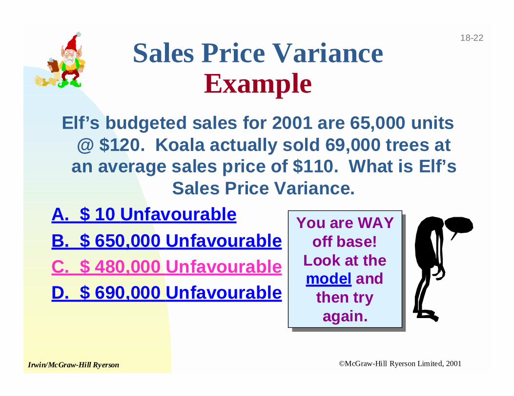
Sales Price VarianceExample
Elf’s budgeted sales for 2001 are 65,000 units@ $120. Koala actually sold 69,000 trees at
an average sales price of $110. What is Elf’sSales Price Variance.
A. $ 10 Unfavourable
B. $ 650,000 Unfavourable
C. $ 480,000 Unfavourable
D. $ 690,000 Unfavourable
You are WAYoff base!
Look at themodel and
then tryagain.
You are WAYoff base!
Look at themodel and
then tryagain.
©McGraw-Hill Ryerson Limited, 2001Irwin/McGraw-Hill Ryerson
18-23
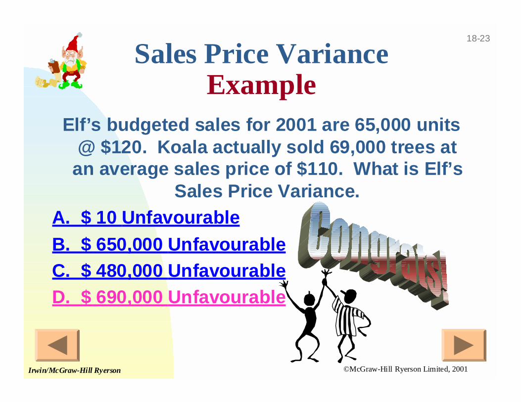
Sales Price VarianceExample
Elf’s budgeted sales for 2001 are 65,000 units@ $120. Koala actually sold 69,000 trees at
an average sales price of $110. What is Elf’sSales Price Variance.
A. $ 10 Unfavourable
B. $ 650,000 Unfavourable
C. $ 480,000 Unfavourable
D. $ 690,000 Unfavourable
©McGraw-Hill Ryerson Limited, 2001Irwin/McGraw-Hill Ryerson
18-24
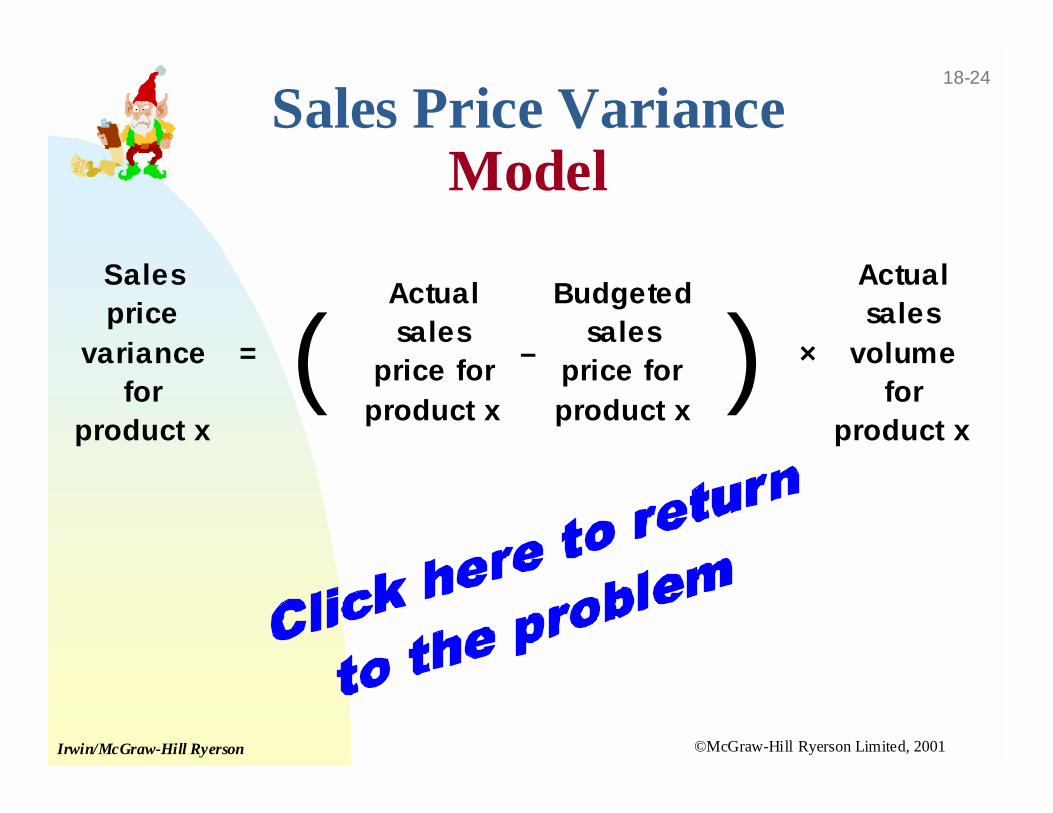
Sales Price VarianceModel
Sales price
variance for
product x
= (Actual sales
price for product x
–
Budgeted sales
price for product x
) ×
Actual sales
volume for
product x

©McGraw-Hill Ryerson Limited, 2001Irwin/McGraw-Hill Ryerson
18-25
Sales Volume VarianceModel
Sales Volume
Variance = (
Actual unit sales volume
for product x
–
Budgeted unit sales volume
for product x
) ×
Budgeted sales
price for product x
This variance measures howmuch of the total revenue
variance is due to unit salesdiffering from budgeted unit
sales.
©McGraw-Hill Ryerson Limited, 2001Irwin/McGraw-Hill Ryerson
18-26
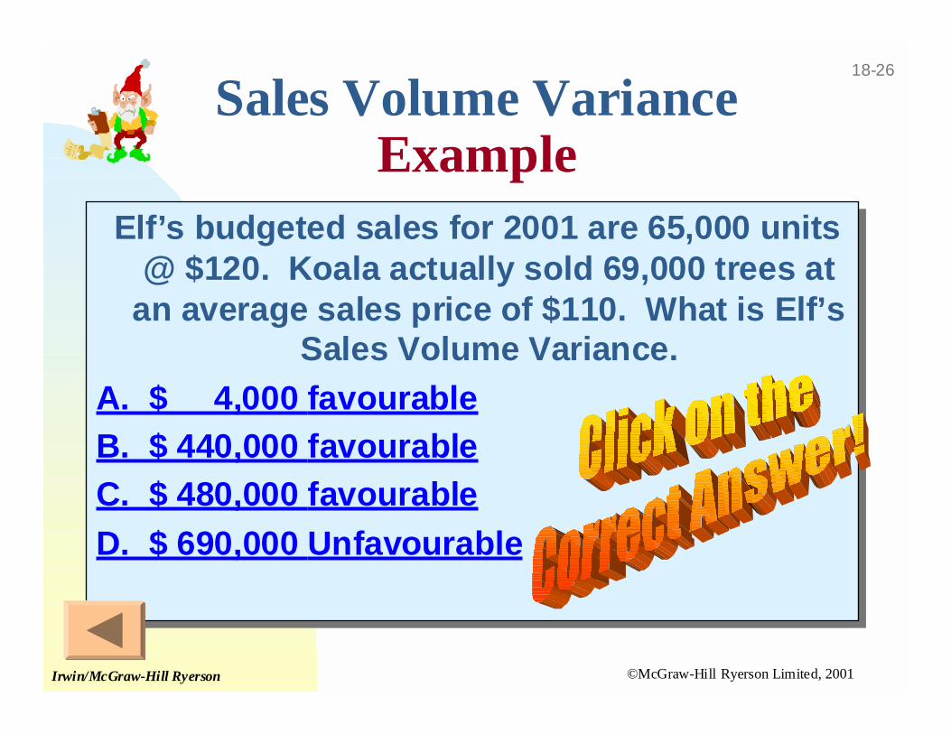
Sales Volume VarianceExample
Elf’s budgeted sales for 2001 are 65,000 units@ $120. Koala actually sold 69,000 trees at
an average sales price of $110. What is Elf’sSales Volume Variance.
A. $ 4,000 favourable
B. $ 440,000 favourable
C. $ 480,000 favourable
D. $ 690,000 Unfavourable
Elf’s budgeted sales for 2001 are 65,000 units@ $120. Koala actually sold 69,000 trees at
an average sales price of $110. What is Elf’sSales Volume Variance.
A. $ 4,000 favourable
B. $ 440,000 favourable
C. $ 480,000 favourable
D. $ 690,000 Unfavourable
©McGraw-Hill Ryerson Limited, 2001Irwin/McGraw-Hill Ryerson
18-27
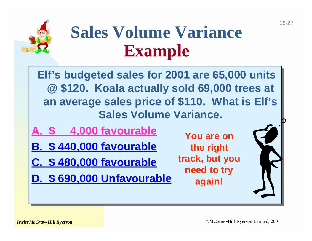
Sales Volume VarianceExample
Elf’s budgeted sales for 2001 are 65,000 units@ $120. Koala actually sold 69,000 trees at
an average sales price of $110. What is Elf’sSales Volume Variance.
A. $ 4,000 favourable
B. $ 440,000 favourable
C. $ 480,000 favourable
D. $ 690,000 Unfavourable
Elf’s budgeted sales for 2001 are 65,000 units@ $120. Koala actually sold 69,000 trees at
an average sales price of $110. What is Elf’sSales Volume Variance.
A. $ 4,000 favourable
B. $ 440,000 favourable
C. $ 480,000 favourable
D. $ 690,000 Unfavourable
You are onthe right
track, but youneed to try
again!
©McGraw-Hill Ryerson Limited, 2001Irwin/McGraw-Hill Ryerson
18-28
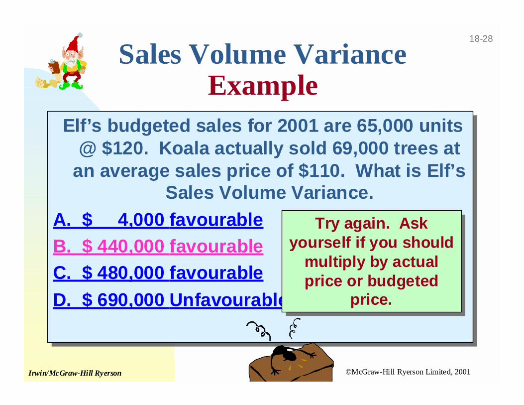
Sales Volume VarianceExample
Elf’s budgeted sales for 2001 are 65,000 units@ $120. Koala actually sold 69,000 trees at
an average sales price of $110. What is Elf’sSales Volume Variance.
A. $ 4,000 favourable
B. $ 440,000 favourable
C. $ 480,000 favourable
D. $ 690,000 Unfavourable
Elf’s budgeted sales for 2001 are 65,000 units@ $120. Koala actually sold 69,000 trees at
an average sales price of $110. What is Elf’sSales Volume Variance.
A. $ 4,000 favourable
B. $ 440,000 favourable
C. $ 480,000 favourable
D. $ 690,000 Unfavourable
Try again. Askyourself if you should
multiply by actualprice or budgeted
price.
Try again. Askyourself if you should
multiply by actualprice or budgeted
price.

©McGraw-Hill Ryerson Limited, 2001Irwin/McGraw-Hill Ryerson
18-29
Sales Volume VarianceExample
Elf’s budgeted sales for 2001 are 65,000 units@ $120. Koala actually sold 69,000 trees at
an average sales price of $110. What is Elf’sSales Volume Variance.
A. $ 4,000 favourable
B. $ 440,000 favourable
C. $ 480,000 favourable
D. $ 690,000 Unfavourable
Elf’s budgeted sales for 2001 are 65,000 units@ $120. Koala actually sold 69,000 trees at
an average sales price of $110. What is Elf’sSales Volume Variance.
A. $ 4,000 favourable
B. $ 440,000 favourable
C. $ 480,000 favourable
D. $ 690,000 Unfavourable
You are WAYoff base!
Look at themodel and
then tryagain.
You are WAYoff base!
Look at themodel and
then tryagain.
©McGraw-Hill Ryerson Limited, 2001Irwin/McGraw-Hill Ryerson
18-30
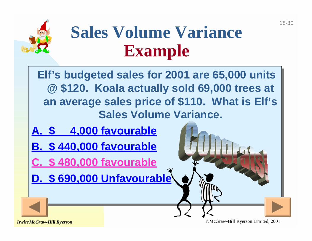
Sales Volume VarianceExample
Elf’s budgeted sales for 2001 are 65,000 units@ $120. Koala actually sold 69,000 trees at
an average sales price of $110. What is Elf’sSales Volume Variance.
A. $ 4,000 favourable
B. $ 440,000 favourable
C. $ 480,000 favourable
D. $ 690,000 Unfavourable
Elf’s budgeted sales for 2001 are 65,000 units@ $120. Koala actually sold 69,000 trees at
an average sales price of $110. What is Elf’sSales Volume Variance.
A. $ 4,000 favourable
B. $ 440,000 favourable
C. $ 480,000 favourable
D. $ 690,000 Unfavourable
©McGraw-Hill Ryerson Limited, 2001Irwin/McGraw-Hill Ryerson
18-31
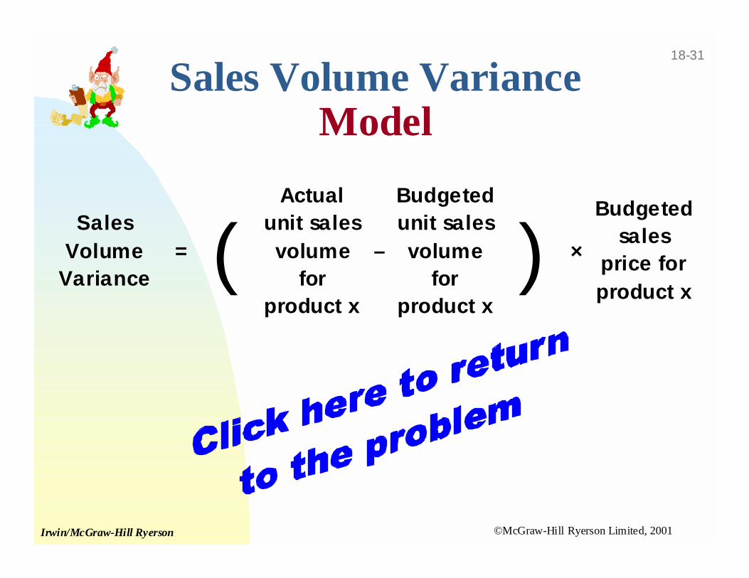
Sales Volume VarianceModel
Sales Volume
Variance = (
Actual unit sales volume
for product x
–
Budgeted unit sales volume
for product x
) ×
Budgeted sales
price for product x
©McGraw-Hill Ryerson Limited, 2001Irwin/McGraw-Hill Ryerson
18-32
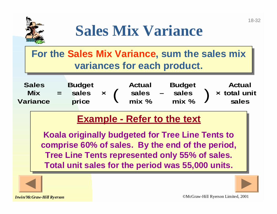
Sales Mix Variance
Sales Mix
Variance =
Budget sales price
× (Actual sales mix %
–Budget sales mix %
) ×Actual
total unit sales
Example - Refer to the text
Koala originally budgeted for Tree Line Tents tocomprise 60% of sales. By the end of the period,Tree Line Tents represented only 55% of sales.Total unit sales for the period was 55,000 units.
Example - Refer to the text
Koala originally budgeted for Tree Line Tents tocomprise 60% of sales. By the end of the period,Tree Line Tents represented only 55% of sales.Total unit sales for the period was 55,000 units.
For the Sales Mix Variance, sum the sales mixvariances for each product.
For the Sales Mix Variance, sum the sales mixvariances for each product.
©McGraw-Hill Ryerson Limited, 2001Irwin/McGraw-Hill Ryerson
18-33
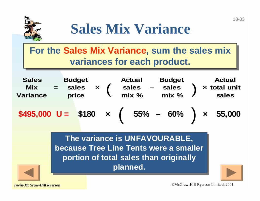
Sales Mix Variance
The variance is UNFAVOURABLE,because Tree Line Tents were a smaller
portion of total sales than originallyplanned.
The variance is UNFAVOURABLE,because Tree Line Tents were a smaller
portion of total sales than originallyplanned.
$495,000 U = $180 × ( 55% – 60% ) × 55,000
Sales Mix
Variance =
Budget sales price
× (Actual sales mix %
–Budget sales mix %
) ×Actual
total unit sales
For the Sales Mix Variance, sum the sales mixvariances for each product.
For the Sales Mix Variance, sum the sales mixvariances for each product.
©McGraw-Hill Ryerson Limited, 2001Irwin/McGraw-Hill Ryerson
18-34
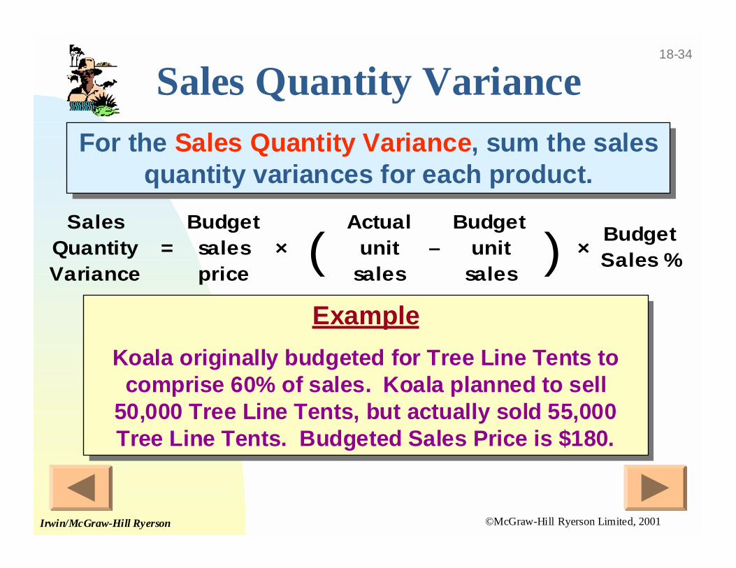
Sales Quantity Variance
Example
Koala originally budgeted for Tree Line Tents tocomprise 60% of sales. Koala planned to sell
50,000 Tree Line Tents, but actually sold 55,000Tree Line Tents. Budgeted Sales Price is $180.
Example
Koala originally budgeted for Tree Line Tents tocomprise 60% of sales. Koala planned to sell
50,000 Tree Line Tents, but actually sold 55,000Tree Line Tents. Budgeted Sales Price is $180.
Sales Quantity Variance
=Budget sales price
× (Actual
unit sales
–Budget
unit sales
) ×Budget Sales %
For the Sales Quantity Variance, sum the salesquantity variances for each product.
For the Sales Quantity Variance, sum the salesquantity variances for each product.
©McGraw-Hill Ryerson Limited, 2001Irwin/McGraw-Hill Ryerson
18-35
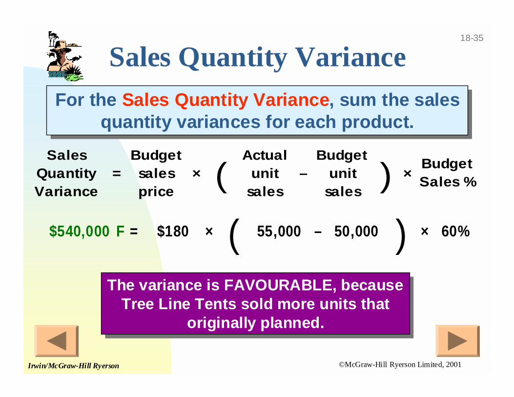
Sales Quantity Variance
Sales Quantity Variance
=Budget sales price
× (Actual
unit sales
–Budget
unit sales
) ×Budget Sales %
For the Sales Quantity Variance, sum the salesquantity variances for each product.
For the Sales Quantity Variance, sum the salesquantity variances for each product.
$540,000 F = $180 × ( 55,000 – 50,000 ) × 60%
The variance is FAVOURABLE, becauseTree Line Tents sold more units that
originally planned.
The variance is FAVOURABLE, becauseTree Line Tents sold more units that
originally planned.
©McGraw-Hill Ryerson Limited, 2001Irwin/McGraw-Hill Ryerson
18-36
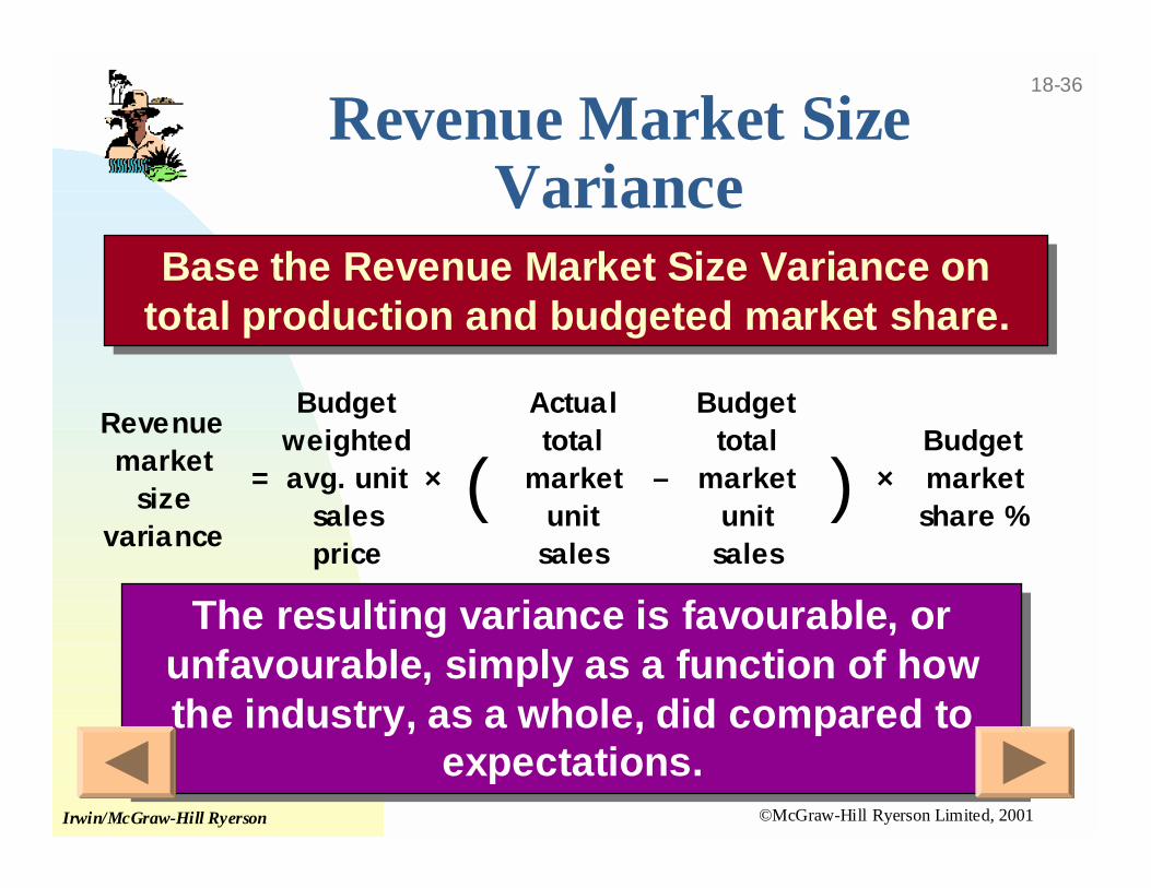
The resulting variance is favourable, orunfavourable, simply as a function of howthe industry, as a whole, did compared to
expectations.
The resulting variance is favourable, orunfavourable, simply as a function of howthe industry, as a whole, did compared to
expectations.
Revenue Market SizeVariance
Base the Revenue Market Size Variance ontotal production and budgeted market share.
Base the Revenue Market Size Variance ontotal production and budgeted market share.
Revenue market
size variance
=
Budget weighted avg. unit
sales price
× (Actual total
market unit
sales
–
Budget total
market unit
sales
) ×Budget market share %
©McGraw-Hill Ryerson Limited, 2001Irwin/McGraw-Hill Ryerson
18-37
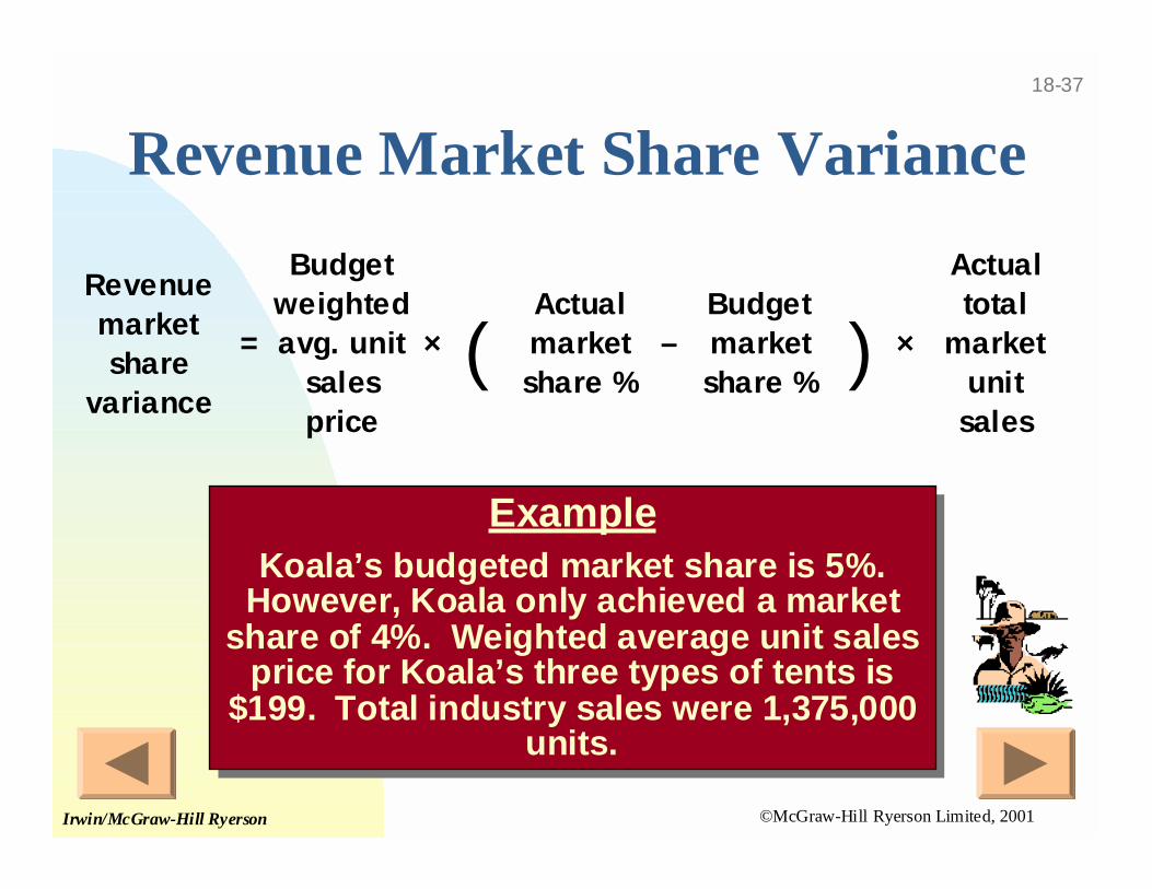
Revenue Market Share Variance
Revenue market share
variance
=
Budget weighted avg. unit
sales price
× (Actual market share %
–Budget market share %
) ×
Actual total
market unit
sales
ExampleKoala’s budgeted market share is 5%.
However, Koala only achieved a marketshare of 4%. Weighted average unit sales
price for Koala’s three types of tents is$199. Total industry sales were 1,375,000
units.
ExampleKoala’s budgeted market share is 5%.
However, Koala only achieved a marketshare of 4%. Weighted average unit sales
price for Koala’s three types of tents is$199. Total industry sales were 1,375,000
units.
©McGraw-Hill Ryerson Limited, 2001Irwin/McGraw-Hill Ryerson
18-38
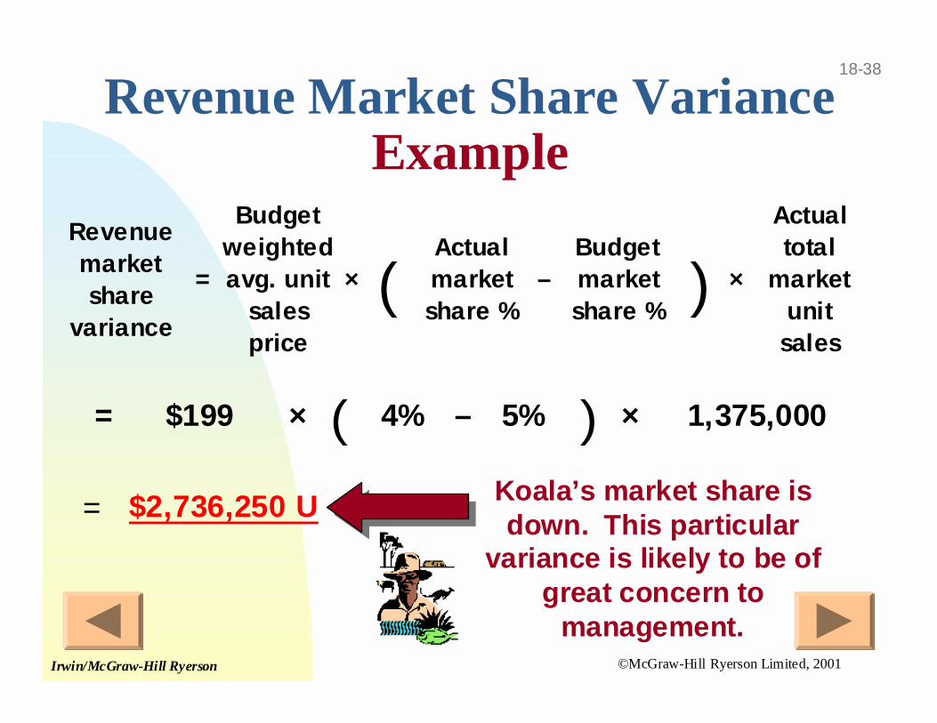
Koala’s market share isdown. This particular
variance is likely to be ofgreat concern to
management.
Revenue Market Share VarianceExample
Revenue market share
variance
=
Budget weighted avg. unit
sales price
× (Actual market share %
–Budget market share %
) ×
Actual total
market unit
sales
= $199 × ( 4% – 5% ) × 1,375,000
= $2,736,250 U
©McGraw-Hill Ryerson Limited, 2001Irwin/McGraw-Hill Ryerson
18-39
©McGraw-Hill Ryerson Limited, 2001Irwin/McGraw-Hill Ryerson
18-40
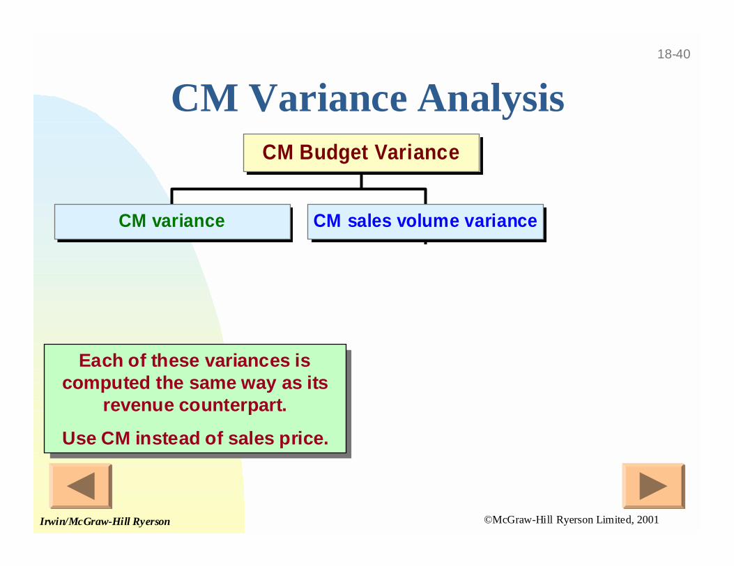
CM Variance Analysis
CM variance CM sales volume variance
CM Budget Variance
Each of these variances iscomputed the same way as its
revenue counterpart.
Use CM instead of sales price.
Each of these variances iscomputed the same way as its
revenue counterpart.
Use CM instead of sales price.
©McGraw-Hill Ryerson Limited, 2001Irwin/McGraw-Hill Ryerson
18-41
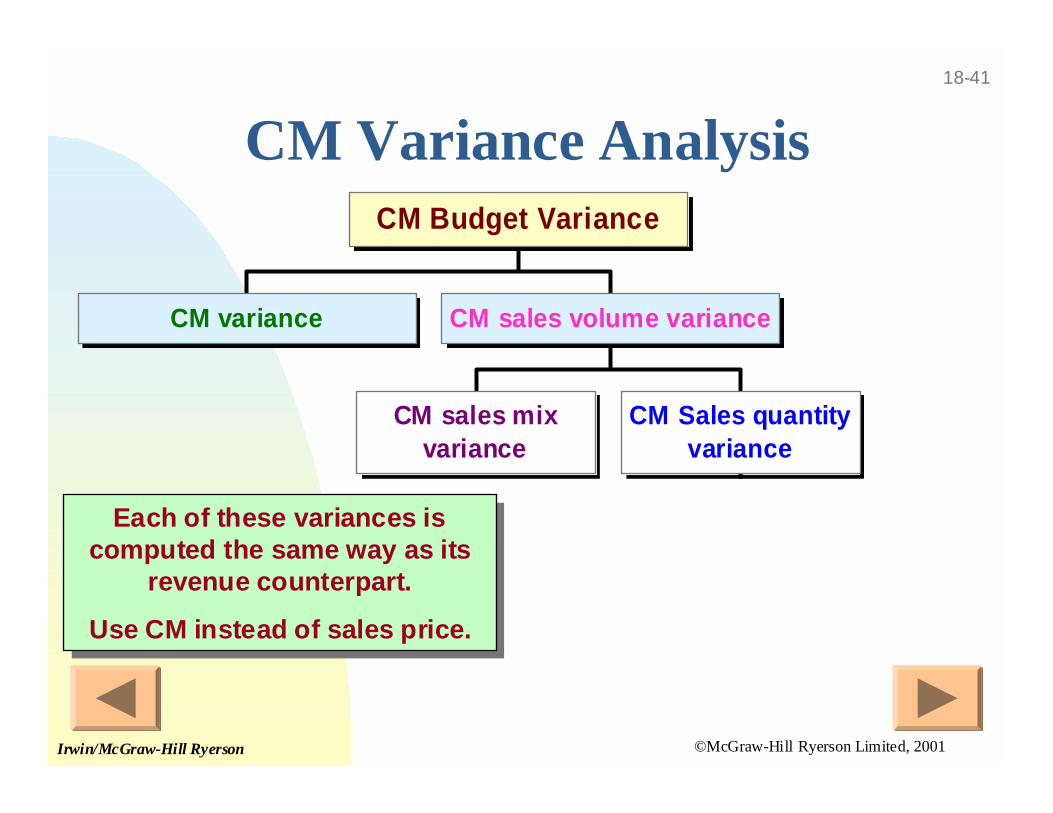
CM Variance Analysis
CM variance
CM sales mixvariance
CM Sales quantityvariance
CM sales volume variance
CM Budget Variance
Each of these variances iscomputed the same way as its
revenue counterpart.
Use CM instead of sales price.
Each of these variances iscomputed the same way as its
revenue counterpart.
Use CM instead of sales price.
©McGraw-Hill Ryerson Limited, 2001Irwin/McGraw-Hill Ryerson
18-42
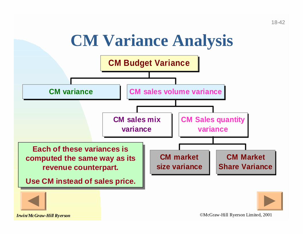
CM Variance Analysis
CM variance
CM sales mixvariance
CM marketsize variance
CM MarketShare Variance
CM Sales quantityvariance
CM sales volume variance
CM Budget Variance
Each of these variances iscomputed the same way as its
revenue counterpart.
Use CM instead of sales price.
Each of these variances iscomputed the same way as its
revenue counterpart.
Use CM instead of sales price.
©McGraw-Hill Ryerson Limited, 2001Irwin/McGraw-Hill Ryerson
18-43
AbsorptionCosting
VariableCostingVs.
Income Reporting Effects ofAlternative Product-Costing
Approaches
©McGraw-Hill Ryerson Limited, 2001Irwin/McGraw-Hill Ryerson
18-44
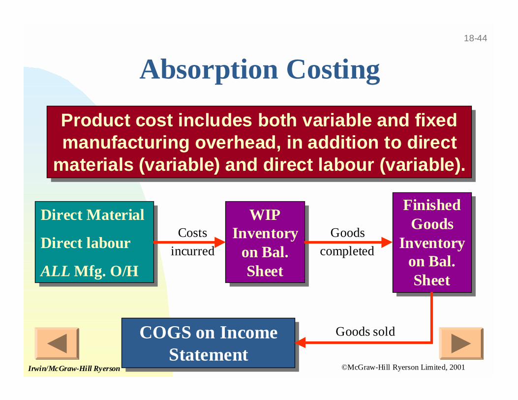
COGS on IncomeStatement
COGS on IncomeStatement
Absorption Costing
Product cost includes both variable and fixedmanufacturing overhead, in addition to direct
materials (variable) and direct labour (variable).
Product cost includes both variable and fixedmanufacturing overhead, in addition to direct
materials (variable) and direct labour (variable).
Direct Material
Direct labour
ALL Mfg. O/H
Direct Material
Direct labour
ALL Mfg. O/H
WIPInventory
on Bal.Sheet
WIPInventory
on Bal.Sheet
FinishedGoods
Inventoryon Bal.Sheet
FinishedGoods
Inventoryon Bal.Sheet
Costs
incurred
Goods
completed
Goods sold
©McGraw-Hill Ryerson Limited, 2001Irwin/McGraw-Hill Ryerson
18-45
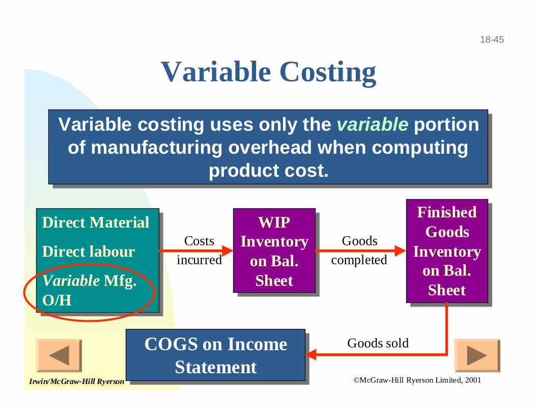
Variable Costing
Variable costing uses only the variable portionof manufacturing overhead when computing
product cost.
Variable costing uses only the variable portionof manufacturing overhead when computing
product cost.
COGS on IncomeStatement
COGS on IncomeStatement
Direct Material
Direct labour
Variable Mfg.O/H
Direct Material
Direct labour
Variable Mfg.O/H
WIPInventory
on Bal.Sheet
WIPInventory
on Bal.Sheet
FinishedGoods
Inventoryon Bal.Sheet
FinishedGoods
Inventoryon Bal.Sheet
Costs
incurred
Goods
completed
Goods sold
©McGraw-Hill Ryerson Limited, 2001Irwin/McGraw-Hill Ryerson
18-46
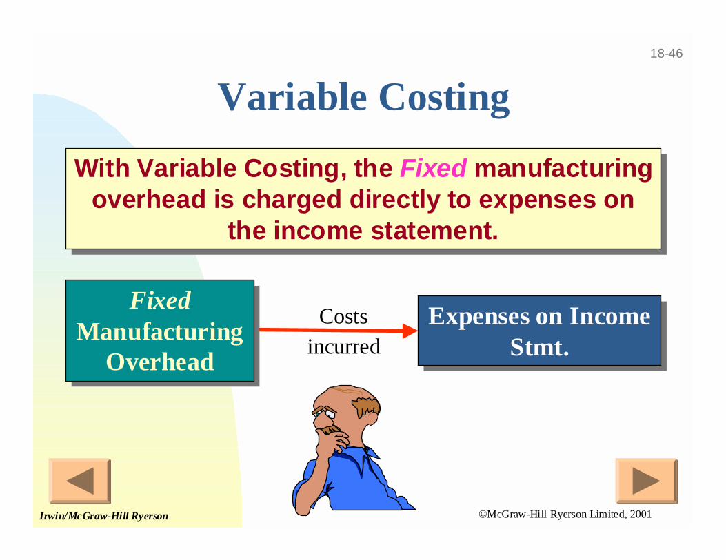
Costs
incurredExpenses on Income
Stmt.
Expenses on IncomeStmt.
Variable Costing
With Variable Costing, the Fixed manufacturingoverhead is charged directly to expenses on
the income statement.
With Variable Costing, the Fixed manufacturingoverhead is charged directly to expenses on
the income statement.
FixedManufacturing
Overhead
FixedManufacturing
Overhead
©McGraw-Hill Ryerson Limited, 2001Irwin/McGraw-Hill Ryerson
18-47
Alternative Product-Costing
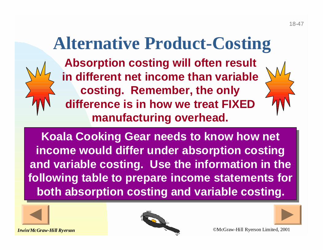
Koala Cooking Gear needs to know how netincome would differ under absorption costing
and variable costing. Use the information in thefollowing table to prepare income statements for
both absorption costing and variable costing.
Koala Cooking Gear needs to know how netincome would differ under absorption costing
and variable costing. Use the information in thefollowing table to prepare income statements for
both absorption costing and variable costing.
Absorption costing will often resultin different net income than variable
costing. Remember, the onlydifference is in how we treat FIXED
manufacturing overhead.
©McGraw-Hill Ryerson Limited, 2001Irwin/McGraw-Hill Ryerson
18-48
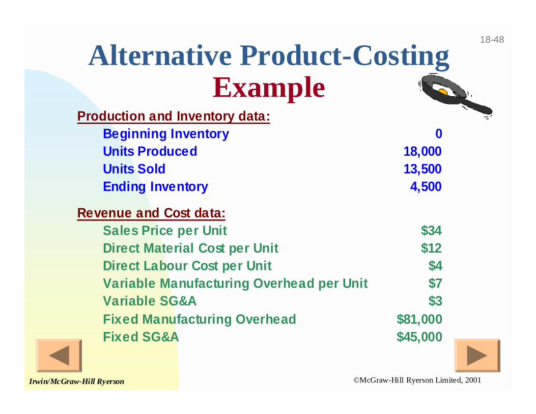
Production and Inventory data:Beginning Inventory 0Units Produced 18,000Units Sold 13,500Ending Inventory 4,500
Revenue and Cost data:Sales Price per Unit $34Direct Material Cost per Unit $12Direct Labour Cost per Unit $4Variable Manufacturing Overhead per Unit $7Variable SG&A $3Fixed Manufacturing Overhead $81,000Fixed SG&A $45,000
Alternative Product-CostingExample
©McGraw-Hill Ryerson Limited, 2001Irwin/McGraw-Hill Ryerson
18-49
Absorption CostingExample
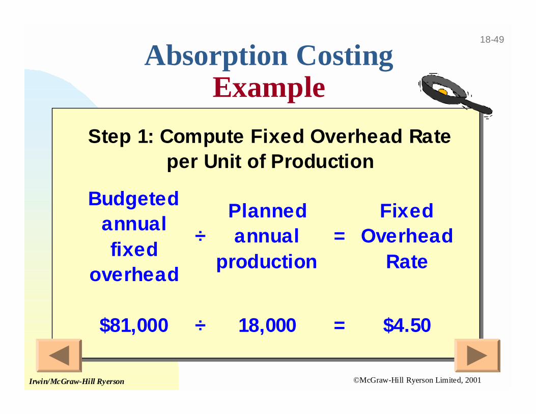
Budgeted annual fixed
overhead
÷Planned annual
production =
Fixed Overhead
Rate
$81,000 ÷ 18,000 = $4.50
Step 1: Compute Fixed Overhead Rate per Unit of Production
©McGraw-Hill Ryerson Limited, 2001Irwin/McGraw-Hill Ryerson
18-50
Absorption CostingExample
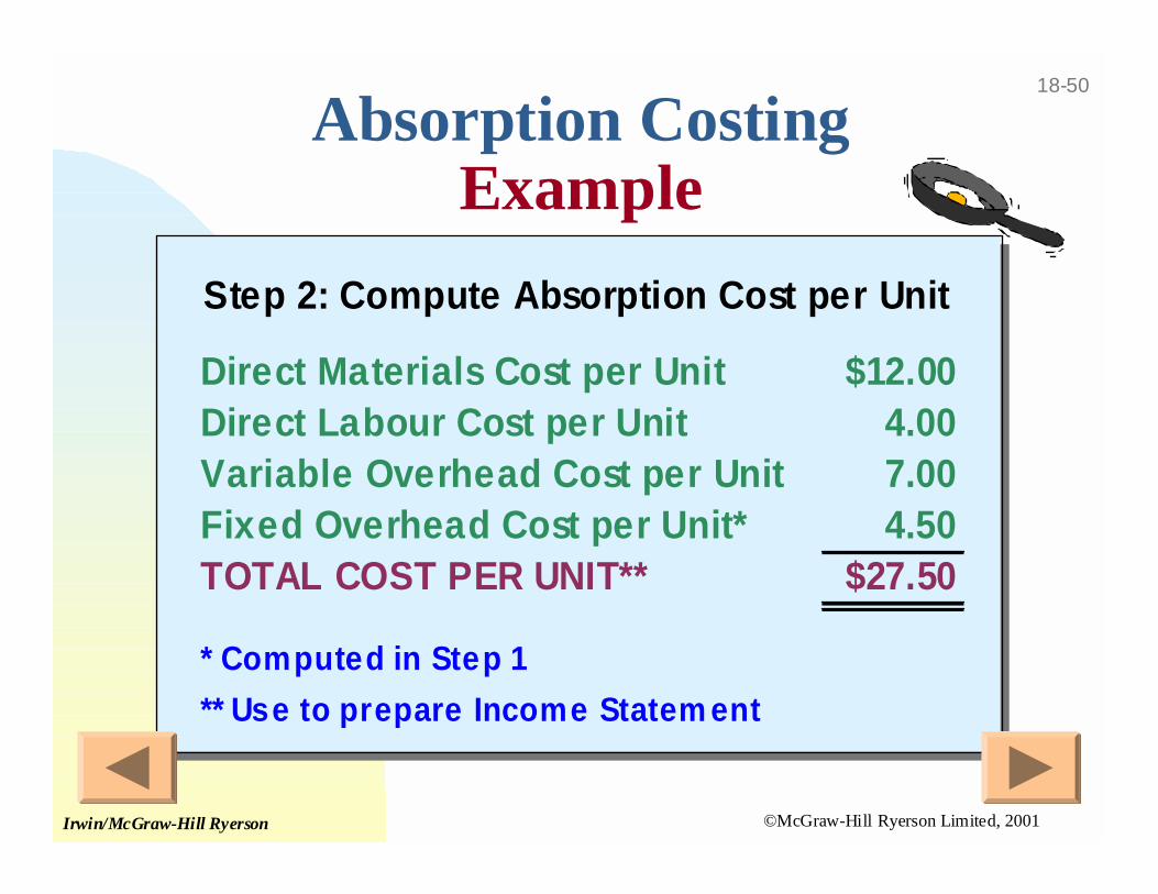
Direct Materials Cost per Unit $12.00Direct Labour Cost per Unit 4.00Variable Overhead Cost per Unit 7.00Fixed Overhead Cost per Unit* 4.50TOTAL COST PER UNIT** $27.50
* Computed in Step 1
** Use to prepare Income Statem ent
Step 2: Compute Absorption Cost per Unit
©McGraw-Hill Ryerson Limited, 2001Irwin/McGraw-Hill Ryerson
18-51
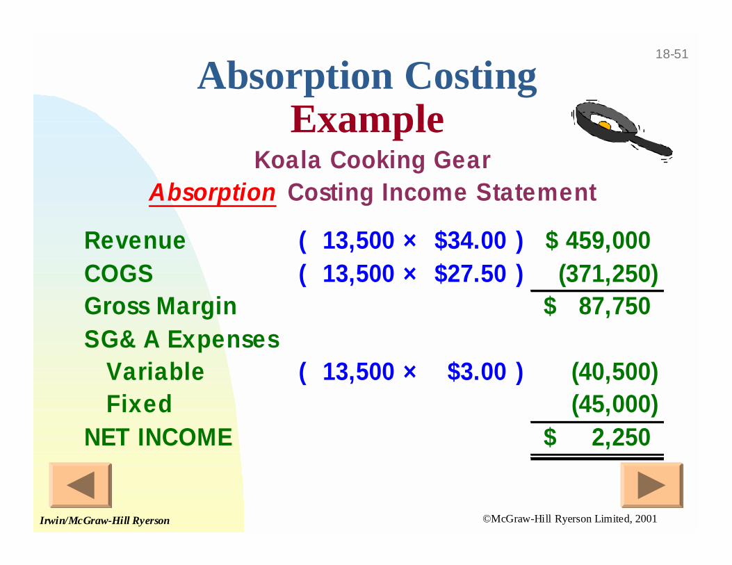
Absorption CostingExample
Revenue ( 13,500 × $34.00 ) 459,000$ COGS ( 13,500 × $27.50 ) (371,250) Gross Margin 87,750$ SG& A Expenses Variable ( 13,500 × $3.00 ) (40,500) Fixed (45,000) NET INCOME 2,250$
Koala Cooking GearAbsorption Costing Income Statement
©McGraw-Hill Ryerson Limited, 2001Irwin/McGraw-Hill Ryerson
18-52
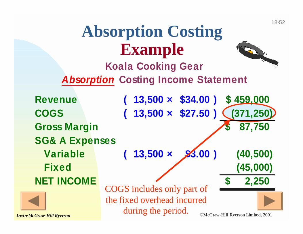
COGS includes only part ofthe fixed overhead incurred
during the period.
Absorption CostingExample
Revenue ( 13,500 × $34.00 ) 459,000$ COGS ( 13,500 × $27.50 ) (371,250) Gross Margin 87,750$ SG& A Expenses Variable ( 13,500 × $3.00 ) (40,500) Fixed (45,000) NET INCOME 2,250$
Koala Cooking GearAbsorption Costing Income Statement
©McGraw-Hill Ryerson Limited, 2001Irwin/McGraw-Hill Ryerson
18-53
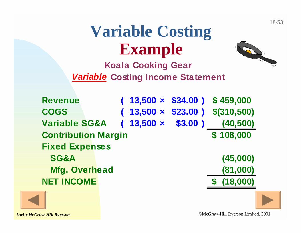
Variable CostingExample
Revenue ( 13,500 × $34.00 ) 459,000$ COGS ( 13,500 × $23.00 ) (310,500)$ Variable SG&A ( 13,500 × $3.00 ) (40,500) Contribution Margin 108,000$ Fixed Expenses SG&A (45,000) Mfg. Overhead (81,000) NET INCOME (18,000)$
Koala Cooking GearVariable Costing Income Statement
©McGraw-Hill Ryerson Limited, 2001Irwin/McGraw-Hill Ryerson
18-54
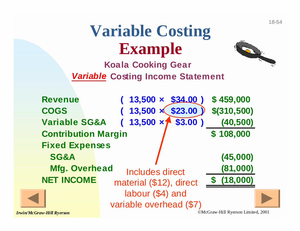
Includes directmaterial ($12), direct
labour ($4) andvariable overhead ($7)
Variable CostingExample
Revenue ( 13,500 × $34.00 ) 459,000$ COGS ( 13,500 × $23.00 ) (310,500)$ Variable SG&A ( 13,500 × $3.00 ) (40,500) Contribution Margin 108,000$ Fixed Expenses SG&A (45,000) Mfg. Overhead (81,000) NET INCOME (18,000)$
Koala Cooking GearVariable Costing Income Statement
©McGraw-Hill Ryerson Limited, 2001Irwin/McGraw-Hill Ryerson
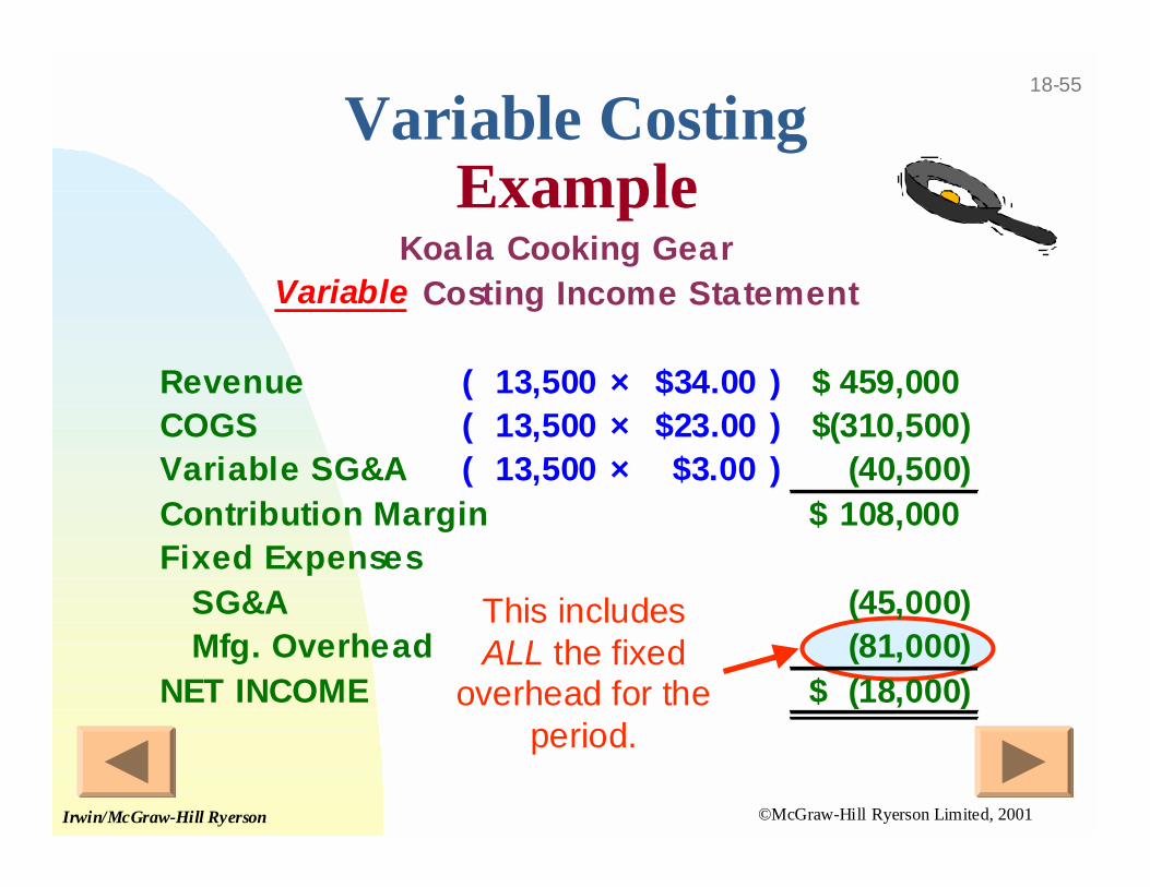
18-55
This includesALL the fixed
overhead for theperiod.
Variable CostingExample
Revenue ( 13,500 × $34.00 ) 459,000$ COGS ( 13,500 × $23.00 ) (310,500)$ Variable SG&A ( 13,500 × $3.00 ) (40,500) Contribution Margin 108,000$ Fixed Expenses SG&A (45,000) Mfg. Overhead (81,000) NET INCOME (18,000)$
Koala Cooking GearVariable Costing Income Statement
©McGraw-Hill Ryerson Limited, 2001Irwin/McGraw-Hill Ryerson
18-56
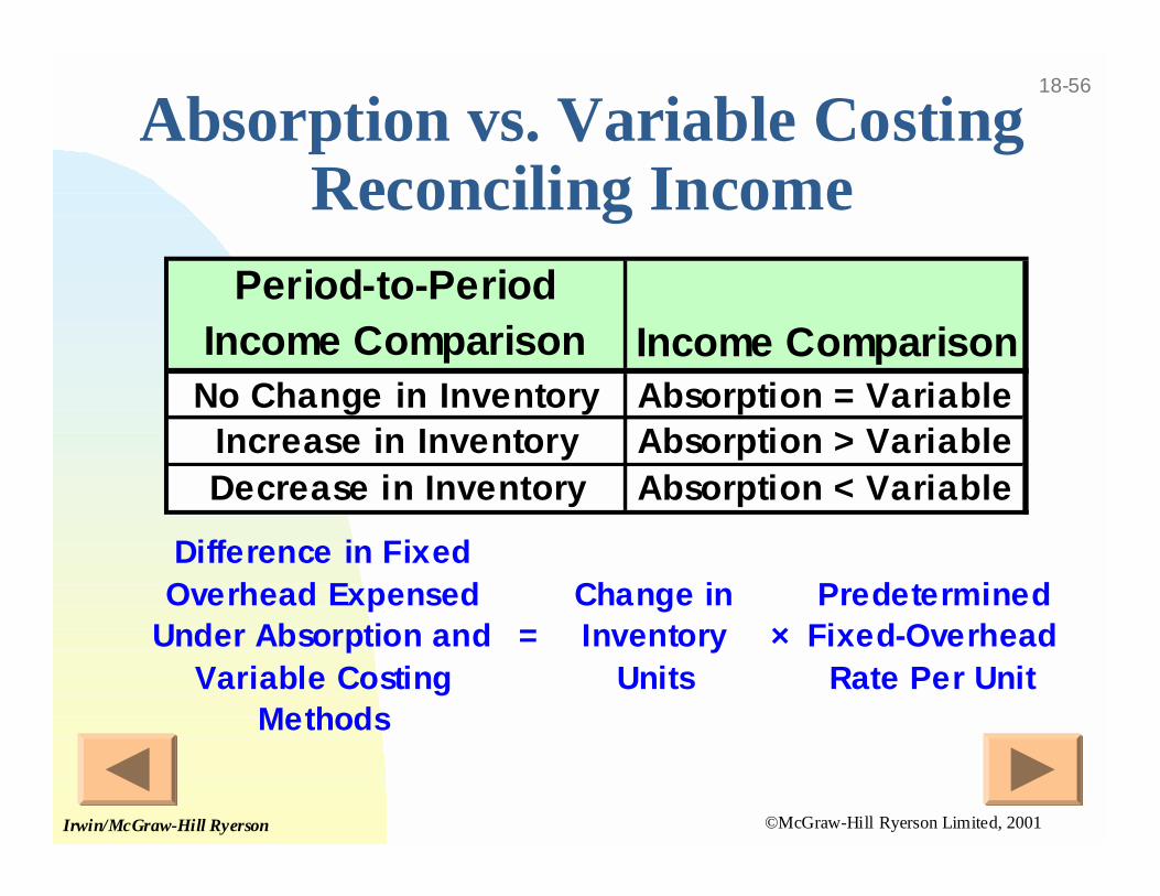
Absorption vs. Variable CostingReconciling Income
Period-to-Period Income Comparison Income Comparison
No Change in Inventory Absorption = VariableIncrease in Inventory Absorption > VariableDecrease in Inventory Absorption < Variable
Difference in Fixed Overhead Expensed
Under Absorption and Variable Costing
Methods
=Change in Inventory
Units×
Predetermined Fixed-Overhead
Rate Per Unit
©McGraw-Hill Ryerson Limited, 2001Irwin/McGraw-Hill Ryerson
18-57
End of Chapter 18
I can’t standit anymore!
Please makeit stop!