cwp-658

CWP-658

Tutorial on seismic interferometry. Part I: Basic

principles and applications

K. Wapenaar1, D. Draganov1, R. Snieder2, X. Campman3 & A. Verdel31Department of Geotechnology, Delft University of Technology, Delft, The Netherlands2Center for Wave Phenomena, Colorado School of Mines, Golden, Colorado 80401, USA3Shell International Exploration and Production B.V., Rijswijk, The Netherlands

ABSTRACT

In part I of this two-part tutorial we explain the basic principles of seismic in-terferometry (also known as Green’s function retrieval) step-by-step and discussits applications. We start with a 1D example (a plane wave propagating alongthe x-axis) and show that the crosscorrelation of the responses at two receiversalong the x-axis gives the Green’s function of the direct wave between these re-ceivers. The 1D analysis continues with the introduction of the different aspectsof interferometry with transient sources (as in exploration seismology) and withnoise sources (as in passive seismology). Next we discuss 2D and 3D direct waveinterferometry and show that the main contributions to the retrieved Green’sfunction come from sources in Fresnel zones around stationary points. The mainapplication of direct wave interferometry is the retrieval of seismic surface waveresponses from ambient noise and the subsequent tomographic determinationof the surface-wave velocity distribution of the subsurface.In a classic paper, Claerbout showed that the autocorrelation of the transmis-sion response of a layered medium gives the reflection response of that medium.This is essentially 1D reflected wave interferometry. We discuss this extensivelyas an introduction to 2D and 3D reflected wave interferometry. One of the mainapplications of reflected wave interferometry is the retrieval of the seismic reflec-tion response from ambient noise and the subsequent imaging of the reflectorsin the subsurface.A common aspect of direct and reflected wave interferometry is that virtualsources are created at positions where there are only receivers, without requiringknowledge of the subsurface medium parameters nor of the positions of theactual sources.

Key words: seismic interferometry

INTRODUCTION

In this two-part tutorial we give an overview of thebasic principles and the underlying theory of seismicinterferometry and discuss applications and new ad-vances. The term “seismic interferometry” refers to theprinciple of generating new seismic responses of virtualsources⋆ by crosscorrelating seismic observations at dif-ferent receiver locations. One can distinguish between

⋆In the literature on seismic interferometry, the term “virtualsource” often refers to the method of Bakulin and Calvert

controlled-source and passive seismic interferometry.Controlled-source seismic interferometry, pioneered bySchuster (2001), Bakulin and Calvert (2004) and others,

(2004, 2006) which is discussed extensively in Part II. Note,

however, that creating a virtual source is the essence of vir-tually all seismic interferometry methods (see e.g. Schuster(2001), who already used this terminology). In this paper(Parts I and II) we use the term “virtual source” wheneverappropriate. When it refers to Bakulin and Calvert’s methodwe will mention this explicitly.

222 K. Wapenaar, et al.

comprises a new processing methodology for seismic ex-ploration data. Apart from crosscorrelation, controlled-source interferometry also involves summation of corre-lations over different source positions. Passive seismicinterferometry, on the other hand, is a methodologyfor turning passive seismic measurements (ambient seis-mic noise or (micro-) earthquake responses) into deter-ministic seismic responses. Here we further distinguishbetween retrieving surface-wave transmission responses(Campillo and Paul, 2003; Shapiro and Campillo, 2004;Sabra et al., 2005a) and exploration-type reflection re-sponses (Claerbout, 1968; Scherbaum, 1987b; Draganovet al., 2007, 2009). In passive interferometry of ambientnoise, no explicit summation of correlations over dif-ferent source positions is required, since the correlatedresponses are a superposition of simultaneously actinguncorrelated sources.

In all cases, the response that is retrieved by cross-correlating two receiver recordings (and summing overdifferent sources) can be interpreted as the responsethat would be measured at one of the receiver loca-tions as if there were a source at the other. Becausesuch a point-source response is equal to a Green’s func-tion convolved with a wavelet, seismic interferometryis also often called “Green’s function retrieval”. Bothterminologies are used in this paper. The term interfer-ometry is borrowed from radio astronomy, in which itrefers to crosscorrelation methods applied to radio sig-nals from distant objects Thompson et al. (2001). Thename Green’s function honors George Green who, in aprivately published essay, introduced the use of impulseresponses in field representations Green (1828). Challisand Sheard (2003) give a brief history of Green’s lifeand theorem. Ramırez and Weglein (2009) review ap-plications of Green’s theorem in seismic processing.

Early successful results of Green’s function retrievalfrom noise correlations were obtained in the field of ul-trasonics Weaver and Lobkis (2001, 2002). The experi-ments were done with diffuse fields in a closed system.Here “diffuse” means that the amplitudes of the nor-mal modes are uncorrelated but have equal expectedenergies. Hence, the crosscorrelation of the field at tworeceiver positions does not contain cross-terms of un-equal normal modes. The sum of the remaining terms isproportional to the modal representation of the Green’sfunction of the closed system Lobkis and Weaver (2001).Hence, the crosscorrelation of a diffuse field in a closedsystem converges to its impulse response. Later it wasrecognized, e.g. Godin (2007), that this theoretical ex-planation is akin to the fluctuation-dissipation theorem(Callen and Welton, 1951; Rytov, 1956; Rytov et al.,1989; Le Bellac et al., 2004).

The Earth is a closed system, but at the scale ofglobal seismology the wavefield is far from diffuse. Atthe scale of exploration seismology, an ambient noisefield may have a diffuse character, but the encompass-ing system is not closed. Hence, for seismic interferome-

try the normal-mode approach breaks down. Through-out this paper we consider seismic interferometry (orGreen’s function retrieval) in open systems, includinghalf-spaces below a free surface. Instead of a treatmentper field of application or a chronological discussion, wehave chosen for a setup in which we explain the prin-ciples of seismic interferometry step by step. In PartI we start with the basic principles of 1D direct-waveinterferometry and conclude with a discussion of theprinciples of 3D reflected-wave interferometry. We dis-cuss applications in controlled-source as well as passiveinterferometry and, where appropriate, we review thehistorical background. To stay focussed on seismic ap-plications, we refrain from a further discussion of thenormal-mode approach, nor do we discuss the many in-teresting applications of Green’s function retrieval inunderwater acoustics (e.g. Roux and Fink (2003), Sabraet al. (2005c), Brooks and Gerstoft (2007)).

DIRECT-WAVE INTERFEROMETRY

1D analysis of direct-wave interferometry

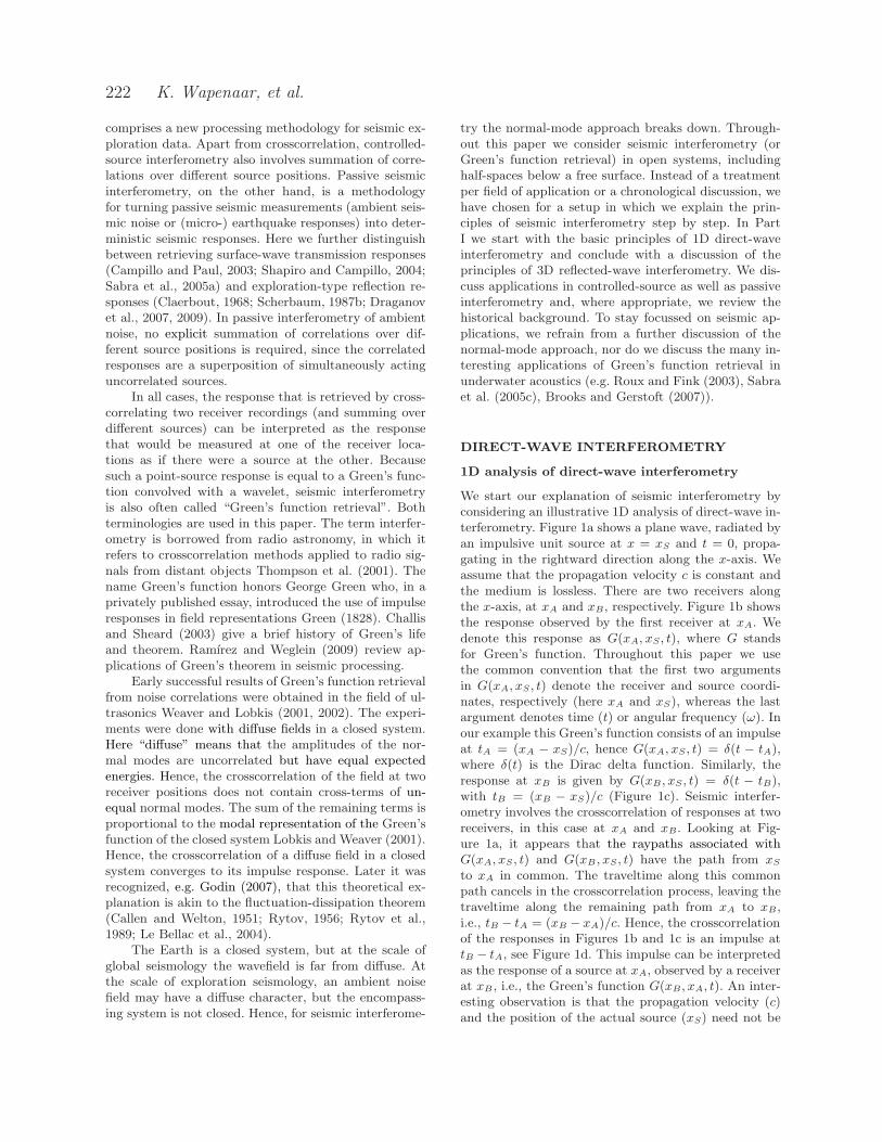
We start our explanation of seismic interferometry byconsidering an illustrative 1D analysis of direct-wave in-terferometry. Figure 1a shows a plane wave, radiated byan impulsive unit source at x = xS and t = 0, propa-gating in the rightward direction along the x-axis. Weassume that the propagation velocity c is constant andthe medium is lossless. There are two receivers alongthe x-axis, at xA and xB, respectively. Figure 1b showsthe response observed by the first receiver at xA. Wedenote this response as G(xA, xS, t), where G standsfor Green’s function. Throughout this paper we usethe common convention that the first two argumentsin G(xA, xS, t) denote the receiver and source coordi-nates, respectively (here xA and xS), whereas the lastargument denotes time (t) or angular frequency (ω). Inour example this Green’s function consists of an impulseat tA = (xA − xS)/c, hence G(xA, xS, t) = δ(t − tA),where δ(t) is the Dirac delta function. Similarly, theresponse at xB is given by G(xB, xS, t) = δ(t − tB),with tB = (xB − xS)/c (Figure 1c). Seismic interfer-ometry involves the crosscorrelation of responses at tworeceivers, in this case at xA and xB. Looking at Fig-ure 1a, it appears that the raypaths associated withG(xA, xS, t) and G(xB , xS, t) have the path from xS

to xA in common. The traveltime along this commonpath cancels in the crosscorrelation process, leaving thetraveltime along the remaining path from xA to xB,i.e., tB − tA = (xB − xA)/c. Hence, the crosscorrelationof the responses in Figures 1b and 1c is an impulse attB − tA, see Figure 1d. This impulse can be interpretedas the response of a source at xA, observed by a receiverat xB , i.e., the Green’s function G(xB, xA, t). An inter-esting observation is that the propagation velocity (c)and the position of the actual source (xS) need not be

Tutorial on seismic interferometry, Part I 223

Ax

Bx

Sx x

t0 At

t0 Bt

t0 B At t

a)

b)

c)

d)

Figure 1. 1D example of direct-wave interferometry. (a) Aplane wave traveling rightward along the x-axis, emitted byan impulsive source at x = xS and t = 0. (b). The responseobserved by a receiver at xA. This is the Green’s functionG(xA, xS , t). (c) As in (b), but for a receiver at xB . (d)Crosscorrelation of the responses at xA and xB. This is in-terpreted as the response of a source at xA, observed at xB,i.e., G(xB , xA, t).

known. The traveltimes along the common path fromxS to xA compensate each other, independent of thepropagation velocity and the length of this path. Simi-larly, if the source impulse would occur at t = tS insteadof at t = 0, the impulses observed at xA and xB wouldbe shifted by the same amount of time, tS, which wouldbe canceled in the crosscorrelation. Hence, also the ab-solute time tS at which the source emits its pulse needsnot be known.

Let us discuss this example a bit more precisely. Wedenote the crosscorrelation of the impulse responses atxA and xB as G(xB, xS, t) ∗G(xA, xS,−t). The asteriskdenotes temporal convolution, but the time-reversal ofthe second Green’s function turns the convolution intoa correlation, defined as G(xB, xS, t) ∗ G(xA, xS,−t) =R

G(xB , xS, t+t′)G(xA, xS, t′)dt′. Substituting the deltafunctions into the right-hand side gives

R

δ(t + t′ −tB)δ(t′− tA)dt′ = δ(t− (tB − tA)) = δ(t− (xB − xA)/c).This is indeed the Green’s function G(xB, xA, t), prop-agating from xA to xB. Since we started this derivationwith the crosscorrelation of the Green’s functions, wehave obtained the following 1D Green’s function repre-sentation

G(xB , xA, t) = G(xB, xS, t) ∗ G(xA, xS,−t). (1)

This representation formulates the principle that thecrosscorrelation of observations at two receivers (xA andxB) gives the response at one of those receivers (xB) as ifthere were a source at the other (xA). It also shows whyseismic interferometry is often called Green’s functionretrieval.

Note that the source is not necessarily an impulse.

If the source function is defined by some wavelet s(t),then the responses at xA and xB can be written asu(xA, xS, t) = G(xA, xS, t) ∗ s(t) and u(xB, xS, t) =G(xB, xS, t) ∗ s(t), respectively. Let Ss(t) be the auto-correlation of the wavelet, i.e., Ss(t) = s(t)∗s(−t). Thenthe crosscorrelation of u(xA, xS, t) and u(xB, xS, t) givesthe right-hand side of equation 1, convolved with Ss(t).This is equal to the left-hand side of equation 1, con-volved with Ss(t), hence

G(xB, xA, t) ∗ Ss(t) = u(xB , xS, t) ∗ u(xA, xS,−t). (2)

In words: if the source function is a wavelet instead ofan impulse, then the crosscorrelation of the responsesat two receivers gives the Green’s function betweenthese receivers, convolved with the autocorrelation ofthe source function. This principle holds true for anysource function, including noise. Figures 2a and 2b showthe responses at xA and xB, respectively, of a bandlim-ited noise source N(t) at xS (the central frequency ofthe noise is 30 Hz; the figures show only 4 s of a total of160 s of noise). In this numerical example the distancebetween the receivers is 1200 m and the propagation ve-locity is 2000 m/s, hence, the traveltime between thesereceivers is 0.6 s. As a consequence, the noise responseat xB in Figure 2b is 0.6 s delayed with respect to theresponse at xA in Figure 2a (similar as the impulse inFigure 1c is delayed with respect to the impulse in Fig-ure 1b). Crosscorrelation of these noise responses gives,analogous to equation 2, the impulse response betweenxA and xB, convolved with SN(t), i.e., the autocorre-lation of the noise N(t). The correlation is shown inFigure 2c, which indeed reveals a bandlimited impulsecentered at t = 0.6 s (the traveltime from xA to xB).Note that from registrations at two receivers of a noisefield from an unknown source in a medium with un-known propagation velocity, we have obtained a ban-dlimited version of the Green’s function. By dividing thedistance between the receivers (1200 m) by the travel-time estimated from the bandlimited Green’s function(0.6 s) we obtain an estimate of the propagation velocitybetween the receivers (2000 m/s). This illustrates thatdirect-wave interferometry can be used for tomographicinversion.

Until now we considered a single plane wave prop-agating in the positive x-direction. In Figure 3a we con-sider the same configuration as in Figure 1a, exceptthat now an impulsive unit source at x = x′

S radi-ates a leftward-propagating plane wave. Figure 3b isthe response at xA, given by G(xA, x′

S, t) = δ(t − t′A),with t′A = (x′

S − xA)/c. Similarly, the response at xB isG(xB, x′

S, t) = δ(t − t′B), with t′B = (x′

S − xB)/c (Fig-ure 3c). The crosscorrelation of these responses givesδ(t − (t′B − t′A)) = δ(t + (xB − xA)/c), which is equalto the time-reversed Green’s function G(xB, xA,−t).Hence, for the configuration of Figure 3a we obtain thefollowing Green’s function representation

G(xB, xA,−t) = G(xB, x′

S, t) ∗ G(xA, x′

S,−t). (3)


0 0.5 1 1.5 2 2.5 3 3.5 4−0.1

−0.08

−0.06

−0.04

−0.02

0

0.02

0.04

0.06

0.08

0.1

0 0.5 1 1.5 2 2.5 3 3.5 4−0.1

−0.08

−0.06

−0.04

−0.02

0

0.02

0.04

0.06

0.08

0.1

−1 −0.8 −0.6 −0.4 −0.2 0 0.2 0.4 0.6 0.8 1−30

−20

−10

0

10

20

30

40

50

( )t s

0 1 2 3

0 1 2 3

-1.0 -0.5 0 0.5

a)

b)

c)

( )t s

( )t s

Figure 2. As in Figure 1, but this time for a noisesource N(t) at xS . (a) The response observed at xA, i.e.,u(xA, xS , t) = G(xA, xS , t) ∗ N(t). (b) As in (a), but for areceiver at xB . (c) The crosscorrelation, which is equal toG(xB , xA, t) ∗ SN (t), with SN (t) the autocorrelation of thenoise.

Ax

Bx

t0

t0

t0

a)

b)

c)

d)

xSx '

At '

Bt '

B At t ' '

Figure 3. As in Figure 1, but this time for a leftward-traveling impulsive plane wave. The crosscorrelation in(d) is interpreted as the time-reversed Green’s functionG(xB , xA,−t).

We can combine equations 1 and 3 as follows

G(xB, xA, t) + G(xB , xA,−t) =2

X

i=1

G(xB, x(i)S , t) ∗ G(xA, x

(i)S ,−t), (4)

where x(i)S for i = 1, 2 stands for xS and x′

S, respectively.For the 1D situation this combination may not seemvery useful. We analyze it here, however, because thisrepresentation better resembles the 2D and 3D represen-tations we encounter later. Note that since G(xB, xA, t)is the causal response of an impulse at t = 0 (meaningit is non-zero only for t > 0), it does not overlap with

Ax

Bx

t0

t0

t

a)

b)

c)

d)

Sx x

At

Bt

B At t

B At t

B At t

B At t 0

At '

Bt '

'' ' '

Sx '

Figure 4. As in Figures 1 and 3, but with simultaneouslyrightward- and leftward-traveling impulsive plane waves. Thecrosscorrelation in (d) contains crossterms which have nophysical meaning.

G(xB, xA,−t) (which is non-zero only for t < 0). Hence,G(xB, xA, t) can be resolved from the left-hand side ofequation 4 simply by extracting the causal part. If thesource function is a wavelet s(t) with autocorrelationSs(t), we obtain, analogous to equation 2,

{G(xB , xA, t) + G(xB , xA,−t)} ∗ Ss(t) =2

X

i=1

u(xB, x(i)S , t) ∗ u(xA, x

(i)S ,−t). (5)

Here G(xB, xA, t) ∗ Ss(t) may have some overlap withG(xB, xA,−t) ∗ Ss(t) for small |t| (depending on thelength of the autocorrelation function Ss(t)). HenceG(xB, xA, t) ∗Ss(t) can be extracted from the left-handside of equation 5, except for small distances |xB −xA|.

The right-hand sides of equations 4 and 5 statethat the crosscorrelation is applied to the responsesof each source separately, after which the summationover the sources is carried out. For impulsive sourcesor transient wavelets s(t) these steps should not be in-terchanged. Let us see why. Suppose the sources at xS

and x′

S would act simultaneously, as illustrated in Fig-ure 4a. Then the response at xA would be given byu(xA, t) =

P2i=1 G(xA, x

(i)S , t) ∗ s(t) and the response

at xB by u(xB, t) =P2

j=1 G(xB, x(j)S , t) ∗ s(t). These

responses are shown in Figures 4b and 4c for an impul-sive source (s(t) = δ(t)). The crosscorrelation of theseresponses, shown in Figure 4d, contains two crosstermsat tB − t′A and t′B − tA which have no physical mean-ing. Hence, for impulsive or transient sources the orderof crosscorrelation and summation matters. This is dif-ferent for noise sources. Consider two simultaneouslyacting noise sources N1(t) and N2(t) at xS and x′

S, re-spectively. Then the responses at xA and xB are givenby u(xA, t) =

P2i=1 G(xA, x

(i)S , t) ∗Ni(t) and u(xB , t) =

P2j=1 G(xB , x

(j)S , t) ∗ Nj(t), respectively, see Figures 5a


and 5b. Note that, because each of these responsesis the superposition of a rightward- and a leftward-propagating wave, the response in Figure 5b is not ashifted version of that in Figure 5a (unlike the responsesin Figures 2a and b). We assume that the noise sourcesare uncorrelated, hence 〈Nj(t) ∗ Ni(−t)〉 = δijSN (t),where δij is the Kronecker delta function and 〈·〉 denotesensemble averaging. In practice the ensemble averagingis replaced by integrating over sufficiently long time. Inthe numerical example the duration of the noise signalsis again 160 s (only 4s of noise is shown in Figures 5aand 5b). For the cross correlation of the responses at xA

and xB we may now write

˙

u(xB, t) ∗ u(xA,−t)¸

=

fi 2X

j=1

2X

i=1

G(xB, x(j)S , t) ∗ Nj(t)

∗G(xA, x(i)S ,−t) ∗ Ni(−t)

fl

=2

X

i=1

G(xB, x(i)S , t) ∗ G(xA, x

(i)S ,−t) ∗ SN (t). (6)

Combining this with equation 4 we finally obtain

{G(xB, xA, t) + G(xB, xA,−t)} ∗ SN (t) =

〈u(xB, t) ∗ u(xA,−t)〉. (7)

This expression shows that the crosscorrelation of twoobserved fields at xA and xB, each of which is the super-position of rightward- and leftward-propagating noisefields, gives the Green’s function between xA and xB

plus its time-reversed version, convolved with the auto-correlation of the noise, see Figure 5c. The crossterms,unlike in Figure 4d, do not contribute because the noisesources N1(t) and N2(t) are uncorrelated.

Miyazawa et al. (2008) applied equation 7 with xA

and xB at different depths along a borehole in the pres-ence of industrial noise, at Cold Lake, Alberta, Canada.By choosing for u different components of multicom-ponent sensors in the borehole, they retrieved separateGreen’s functions for P - and S-waves, the latter withdifferent polarizations. From the arrival times in theGreen’s functions they derived the different propagationvelocities and were able to accurately quantify shear-wave splitting.

Despite the relative simplicity of our 1D analysisof direct-wave interferometry, we can make a numberof observations about seismic interferometry that alsohold true for more general situations:

• We can distinguish between interferometry for im-pulsive or transient sources on the one hand (equations4 and 5) and interferometry for noise sources on theother hand (equation 7). In the case of impulsive or tran-sient sources, the responses of each of these sources mustbe crosscorrelated separately, after which a summationover the sources takes place. In the case of uncorrelatednoise sources a single crosscorrelation suffices.

• It appears that an isotropic illumination of the

0 0.5 1 1.5 2 2.5 3 3.5 4−0.1

−0.08

−0.06

−0.04

−0.02

0

0.02

0.04

0.06

0.08

0.1

0 0.5 1 1.5 2 2.5 3 3.5 4−0.1

−0.08

−0.06

−0.04

−0.02

0

0.02

0.04

0.06

0.08

0.1

−1 −0.8 −0.6 −0.4 −0.2 0 0.2 0.4 0.6 0.8 1−10

−5

0

5

10

15

20

0 1 2 3

0 1 2 3

-1.0 -0.5 0 0.5

a)

b)

c)

( )t s

( )t s

( )t s

Figure 5. As in Figure 4, but this time with simultaneouslyrightward- and leftward-traveling uncorrelated noise fields.The crosscorrelation in (c) contains no crossterms.

receivers is required to obtain a time-symmetric re-sponse between the receivers (of which the causal partis the actual response). In 1D, “isotropic illumination”means equal illumination by rightward- and leftward-propagating waves. In 2D and 3D it means equal illu-mination from all directions (discussed in next subsec-tion).

• Instead of the time-symmetric responseG(xB, xA, t) + G(xB , xA,−t), in the literaturewe often encounter an anti-symmetric responseG(xB, xA, t) − G(xB, xA,−t). This is merely a result ofdifferently defined Green’s functions. Note that a simpletime differentiation of the Green’s functions would turnthe symmetric response into an anti-symmetric oneand vice versa (see Wapenaar and Fokkema (2006) fora more detailed discussion on this aspect).

2D and 3D analysis of direct-wave

interferometry

We extend our discussion of direct-wave interferometryto configurations with more dimensions. In the followingwe mainly use heuristic arguments, illustrated with anumerical example. For a more precise derivation, basedon stationary-phase analysis, we refer to Snieder (2004).

Consider the 2D configuration shown in Figure 6a.The horizontal dashed line corresponds to the 1D con-figuration of Figure 1a, with two receivers at xA andxB, 1200 m apart (the boldface x denotes a Carte-sian coordinate vector). The propagation velocity c is2000 m/s and the medium is again assumed to be loss-


−3000 −2000 −1000 0 1000 2000 3000−3000

−2000

−1000

0

1000

2000

3000

S

o

0

o

90

o

180

o

90!

Ax

Bx

a)

−50 0 50 100 150 200 250

0

0.2

0.4

0.6

0.8

1

1.2

1.4

1.6

1.8

2

-90 0 90 180 270

S

1.0

1.5

2.0

0

0.5

t

b)

−50 0 50 100 150 200 250

0

0.2

0.4

0.6

0.8

1

1.2

1.4

1.6

1.8

2

-90 0 90 180 270

S

1.0

1.5

2.0

0

0.5

t

c)

−1 −0.8 −0.6 −0.4 −0.2 0 0.2 0.4 0.6 0.8 1

−1

−0.8

−0.6

−0.4

−0.2

0

0.2

0.4

0.6

0.8

1−50 0 50 100 150 200 250

−1

−0.8

−0.6

−0.4

−0.2

0

0.2

0.4

0.6

0.8

1

-90 0 90 180 270

S

0

0.5

1.0

-1.0

-0.5

t

0

0.5

1.0

-1.0

-0.5

t

d) e)

−300 −200 −100 0 100 200 300

−0.8

−0.6

−0.4

−0.2

0

0.2

0.4

0.6

0.8

1

f)

0

0.5

1.0

-1.0

-0.5

t

Figure 6. 2D example of direct-wave interferometry. (a) Distribution of point sources, isotropically illuminating the receivers

at xA and xB. The thick dashed lines indicate the Fresnel zones. (b) Responses at xA as a function of the (polar) sourcecoordinate φS . (c) Responses at xB . (d) Crosscorrelation of the responses at xA and xB . The dashed lines indicate again theFresnel zones. (e) The sum of the correlations in (d). This is interpreted as {G(xB ,xA, t) + G(xB ,xA,−t)} ∗ Ss(t). The maincontributions come from sources in the Fresnel zones indicated in (a) and (d). (f) Single crosscorrelation of the responses at xA

and xB of simultaneously acting uncorrelated noise sources. The duration of the noise signals was 9600 s.


less. Instead of plane-wave sources, we have many pointsources denoted by the small black dots, distributed overa “pineapple slice”, emitting transient signals with acentral frequency of 30 Hz. In polar coordinates, the po-sitions of the sources are denoted by (rS, φS). The angleφS is equidistantly sampled (∆φS = 0.25o), whereas thedistance rS to the center of the slice is chosen randomlybetween 2000 and 3000 m. The responses at the two re-ceivers at xA and xB are shown in Figures 6b and 6c,respectively, as a function of the (polar) source coor-dinate φS (for display purposes, only every 16th traceis shown). These responses are crosscorrelated (for eachsource separately) and the crosscorrelations are shownin Figure 6d, again as a function of φS. Such a gather isoften called a “correlation gather”. Note that the trav-eltimes in this correlation gather vary smoothly withφS , despite the randomness of the traveltimes in Fig-ures 6b and 6c. This is because in the crosscorrelationprocess only the time difference along the paths to xA

and xB matters. Note that the source in Figure 6a withφS = 0o plays the same role as the plane-wave sourceat xS in Figure 1a. For this source the crosscorrelationgives a signal at |xB − xA|/c = 0.6 s, which is seenin the trace at φS = 0o in Figure 6d. Similarly, thesource at φS = 180o plays the same role as the plane-wave source at x′

S in Figure 3a and leads to the traceat φS = 180o in Figure 6d with a signal at −0.6 s.Analogous to equation 5 we sum the crosscorrelationsof all sources, that is, we sum all traces in Figure 6d,which leads to the time-symmetric response in Figure6e, with two events at 0.6 and −0.6s. These two eventsare again interpreted as the response of a source atxA, observed at xB, plus its time-reversed version, i.e.,{G(xB ,xA, t) + G(xB,xA,−t)} ∗ Ss(t), where Ss(t) isthe autocorrelation of the source wavelet. Because thesources have a finite frequency content, not only thesources exactly at φS = 0o and φS = 180o contributeto these events, but also the sources in Fresnel zonesaround these angles. These Fresnel zones are denotedby the thick dashed lines in Figures 6a and 6d. In Fig-ure 6d it can be seen that the centers of these Fresnelzones are the stationary points of the traveltime curve ofthe crosscorrelations. Note that the events in all tracesoutside the Fresnel zones in Figure 6d interfere destruc-tively and hence give no coherent contribution in Figure6e. The noise between the two events in Figure 6e is dueto the fact that the traveltime curve in Figure 6d is not100 % smooth because of the randomness of the sourcepositions in Figure 6a.

The response in Figure 6e has been obtainedby summing crosscorrelations of independent transientsources. Using the same arguments as in the previoussubsection, we can replace the transient sources by si-multaneously acting noise sources. The crossterms dis-appear when the noise sources are uncorrelated, hence,a single crosscorrelation of noise observations at xA

and xB gives, analogous to equation 7, {G(xB ,xA, t) +

G(xB,xA,−t)} ∗SN (t), where SN(t) is the autocorrela-tion of the noise, see Figure 6f. Note that the symmetryof the responses in Figures 6e and 6f relies again on theisotropic illumination of the receivers, i.e., on the netpower-flux of the illuminating wavefield being (close to)zero (van Tiggelen, 2003; Malcolm et al., 2004; Sanchez-Sesma et al., 2006; Snieder et al., 2007; Perton et al.,2009; Weaver et al., 2009; Yao et al., 2009).

Of course what has been demonstrated here for a2D distribution of sources also holds for a 3D sourcedistribution. In that case all sources in Fresnel volumesrather than Fresnel zones contribute to the retrievalof the direct wave between xA and xB . Furthermore,the sources (in 2D or 3D) are not necessarily primarysources, but can also be secondary sources, i.e., scat-terers in a homogeneous embedding. These secondarysources are not independent, but the late coda of themultiply scattered response reasonably resembles a dif-fuse wave field. Hence, in situations with few primarysources but many secondary sources only the late codais used for Green’s function retrieval Campillo and Paul(2003). It is, however, not clear how well a scatteringmedium should be illuminated by different sources forthe scatterers to act as independent secondary sources.Fan and Snieder (2009) show an example where thescattered waves excited by a single source are equipar-titioned, in the sense that energy propagates equally inall directions, but where the crosscorrelation of thosescattered waves does not resemble the Green’s functionat all.

One of the most widely used applications of direct-wave interferometry is the retrieval of seismic surfacewaves between seismometers and the subsequent to-mographic determination of the surface-wave velocitydistribution of the subsurface. This approach has beenpioneered by Campillo and Paul (2003), Shapiro andCampillo (2004), Sabra et al. (2005b,a) and Shapiro etal. (2005). In layered media, surface waves consist ofseveral propagating modes, of which the fundamentalmode is usually the strongest. As long as only the fun-damental mode is considered, surface waves can be seenas an approximate solution of a 2D wave equation witha frequency-dependent propagation velocity. Hence, byconsidering the 2D configuration of Figure 6a as a planview, the analysis above holds for ambient surface-wavenoise. The Green’s function of the fundamental mode ofthe direct surface wave can thus be extracted by cross-correlating ambient noise recordings at two seismome-ters. When many seismometers are available, this canbe repeated for any combination of two seismometers.In other words, each seismometer can be turned into avirtual source, the response of which is observed by allother seismometers.

Figure 7, reproduced with permission from Lin etal. (2009), shows a beautiful example of the Rayleigh-wave response of a virtual source, southeast of LakeTahoe, California. The white triangles represent over


Figure 7. Two snapshots of the Rayleigh-wave response of a virtual source (the white star), southeast of Lake Tahoe, CaliforniaLin et al. (2009). The white triangles represent over 400 seismometers (USArray stations). The shown response was obtainedby crosscorrelating three years of ambient noise, recorded at the station denoted by the star, with that recorded at all otherstations.

400 seismometers (USArray stations). Ocean-generatedambient seismic noise (Longuet-Higgins, 1950; Webb,1998; Stehly et al., 2006) was recorded between Octo-ber 2004 and November 2007. Since this noise is comingfrom the ocean, it is far from isotropic. This means thatthe crosscorrelation of the noise between any two sta-tions does not yield time-symmetric results like those inFigure 6. However, as long as one of the Fresnel zones issufficiently covered with sources, it is possible to retrieveeither G(xB,xA, t)∗SN (t) or G(xB,xA,−t)∗SN (t) (notethat the location and shape of the Fresnel zone is dif-ferent for each combination of stations). The snapshotsshown in Figures 7a and 7b were obtained by cross-correlating the noise recorded at the station denotedby the star with that recorded at all other stations.The amplitudes exhibit azimuthal variation due to theanisotropic illumination. Responses like this are usedfor tomographic inversion of the Rayleigh-wave veloc-ity of the crust and for the measurement of azimuthalanisotropy in the crust.

Bensen et al. (2007) have shown that it is possibleto retrieve the Rayleigh-wave velocity as a function offrequency. Brenguier et al. (2007) have combined theseapproaches to 3D tomographic inversion. From noisemeasurements at the Piton de la Fournaise volcano theyretrieved the Rayleigh-wave group velocity distributionas a function of frequency and used this to derive a 3DS-wave velocity model of the interior of the volcano.In the past couple of years the applications of directsurface-wave interferometry have expanded spectacu-larly. Without any claim of completeness, we mentionLarose et al. (2005, 2006), Gerstoft et al. (2006), Yao et

al. (2006, 2008), Kang and Shin (2006), Bensen et al.(2008), Gouedard et al. (2008a,b), Liang and Langston(2008), Lin et al. (2008), Ma et al. (2008), Li et al. (2009)and Picozzi et al. (2009). The success of these applica-tions is explained by the fact that surface waves are byfar the strongest events in ambient seismic noise. In thenext section we show that the retrieval of reflected wavesfrom ambient seismic noise is an order more difficult.

Note that direct surface-wave interferometry has aninteresting link with early work by Aki (1957, 1965) andToksoz (1964) on the spatial autocorrelation method(SPAC). The SPAC method employs a circular ar-ray of seismometers, plus a seismometer at the cen-ter of the circle. Assuming a distribution of uncorre-lated fundamental-mode Rayleigh waves, propagatingas plane waves in all directions, the spatial autocor-relation function obtained from the circular array re-veals the local surface-wave velocity as a function offrequency and, subsequently, the local depth-dependentvelocity profile. An important difference with the inter-ferometry approach is that the distances between thereceivers in the SPAC method are usually smaller thanhalf a wavelength Henstridge (1979), making it a localmethod, whereas in direct-wave interferometry the dis-tances are assumed much larger than the wavelength be-cause otherwise the stationary-phase arguments wouldnot hold. More recent discussions on the SPAC methodare given by Okada (2003, 2006) and Asten (2006). Aninteresting discussion on the relation between the SPACmethod and seismic interferometry is given by Yokoi andMargaryan (2008).


a) b) c)

Figure 8. Basic principle of reflected-wave interferometry

Schuster (2001, 2009). (a) A subsurface source emits a waveto the surface where it is received by a geophone. (b) A sec-ond geophone receives a reflected wave. (c) Crosscorrelationeliminates the propagation along the path from the source tothe first geophone. The result is interpreted as the reflectionresponse of a source at the position of the first geophone,observed by the second geophone.

REFLECTED-WAVE INTERFEROMETRY

1D analysis of reflected-wave interferometry

The figure on the cover of Schuster’s book on seismicinterferometry Schuster (2009), reproduced in Figure 8,explains the basic principle of reflected wave interfer-ometry very well. Figure 8a shows a source in the sub-surface which radiates a transient wave to the Earth’ssurface, where it is received by a geophone. The tracecontains the delayed source wavelet. Figure 8b showshow the wave is reflected downward by the surface, re-flected upward again by a scatterer in the subsurface,and received by a second geophone at the Earth’s sur-face. The trace contains the wavelet, which is further de-layed due to the propagation along the additional pathfrom receiver 1 via the scatterer to receiver 2. The prop-agation paths in Figures 8a and 8b have the path fromthe subsurface source to the first receiver in common. Bycrosscorrelating the two traces (Schuster denotes this by⊗), the propagation along this common path is elimi-nated, leaving the path from receiver 1 via the scattererto receiver 2 (Figure 8c). Hence, the result can be inter-preted as a reflection experiment with a source at theposition of the first geophone, of which the reflectionresponse is received by the second geophone.

Let us see how this method deals with multiple re-flections. To this end we consider a configuration con-sisting of a homogeneous lossless layer, sandwiched be-tween a free surface and a homogeneous lossless half-space, see Figure 9a. An impulsive unit source in thelower half-space emits a vertically upward-propagatingplane wave, which reaches the surface after a time t0.Since it was transmitted by a single interface on its wayto the surface, the first arrival is given by τδ(t − t0),

a)

tt

0

( )T t

b)

0t

3r !"

5r !"

r!"

2r ! 4

r ! 6r !

!

r

r"

1"

!

t

( )R t ( )R t

( )t!

t"

0

r r 3r

3r

5r

5r

2r

2r4

r4r 6

r6r

c)

( )t! ( )R t ( )R t

( )T t

d)

Figure 9. From transmission to reflection response (1D). (a)Simple layered medium with an upgoing plane wave radiatedby a source in the lower half-space. (b) The transmission re-sponse T (t), observed at the free surface. (c) The autocorre-lation T (t) ∗ T (−t). The causal part is, apart from a minussign, the reflection response R(t). (d) Configuration, used toderive the same relation for an arbitrarily layered medium.

where τ is the transmission coefficient of the interface(we use lower-case symbols for local transmission andreflection coefficients). This arrival is represented bythe impulse at t = t0 in Figure 9b. The wave is re-


flected downward by the free surface (reflection coef-ficient −1) and subsequently reflected upward by theinterface (reflection coefficient r). Hence, the next ar-rival reaching the surface is −rτδ(t − t0 − ∆t), with∆t = 2∆z/c, where ∆z is the thickness of the firstlayer and c its propagation velocity. Figure 9b showsthe total upgoing wavefield reaching the free surface.It is denoted as T (t), where capital T stands for theglobal transmission response. It consists of an infiniteseries of impulses with regular intervals ∆t (startingat t0), and amplitudes a0 = τ , a1 = −rτ , a2 = r2τ ,a3 = −r3τ , etc. Seismic interferometry for a verticallypropagating plane wave reduces to evaluating the au-tocorrelation of the global transmission response, henceT (t) ∗ T (−t). We obtain the simplest result if we con-sider so-called “power-flux normalized” up- and down-going waves (Frasier, 1970; Kennett et al., 1978; Ursin,1983; Chapman, 1994). This simply means that we de-fine the local transmission coefficient τ as the square-root of the product of the transmission coefficients foracoustic pressure and particle velocity. Hence, for an up-going wave, τ =

p

(1 − r)(1 + r) =√

1 − r2 (which isby the way also the transmission coefficient for a down-going wave). The autocorrelation for zero time-lag is(a2

0+a21+a2

2+a23+···)δ(t) = τ 2(1+r2+r4+r6+···)δ(t) =

τ 2(1 − r2)−1δ(t) = δ(t). This is represented by the im-pulse at t = 0 in Figure 9c. The autocorrelation fortime-lag ∆t is (a1a0 + a2a1 + a3a2 + · · ·)δ(t − ∆t) =−rτ 2(1+ r2 + r4 + · · ·)δ(t−∆t) = −rδ(t−∆t), which isrepresented by the impulse at ∆t in Figure 9c. For time-lags 2∆t, 3∆t etc. we obtain r2δ(t−2∆t), −r3δ(t−3∆t),etc. Apart from an overall minus-sign, these impulsestogether (except the one at t = 0) represent the globalreflection response R(t) of a downgoing plane wave, il-luminating the medium from the free surface. Hence,the causal part of the autocorrelation is equal to −R(t).Similarly, the acausal part is −R(−t). Taking everythingtogether, we have T (t) ∗ T (−t) = δ(t) − R(t) − R(−t),or

R(t) + R(−t) = δ(t) − T (t) ∗ T (−t). (8)

This expression shows that the global reflection re-sponse can be obtained from the autocorrelation of theglobal transmission response. This can be understoodintuitively if one bears in mind that the reflection re-sponse, including all its multiples, is implicitly presentin the coda of the transmission response, see Figure9b. Note the analogy of equation 8 with the expres-sion for direct-wave interferometry, equation 4. In bothcases the left-hand side is a superposition of a causalresponse and its time-reversed version. The main dif-ference is that the right-hand side of equation 4 isa superposition of crosscorrelations of rightward- andleftward-propagating waves, which was necessary to getthe time-symmetric response, whereas the right-handside of equation 8 is a single autocorrelation. Note, how-ever, that the free surface in Figure 9a acts as a mir-

ror, which removes the requirement of having sources atboth sides of the receivers to obtain a time-symmetricresponse.

It can easily be shown that equation 8 holds forarbitrary horizontally layered media. To this end con-sider the configuration shown in Figure 9d. Here theilluminating wavefield is an impulsive downgoing planewave at the free surface (denoted by δ(t) in Figure 9d).The upgoing wave arriving at the free surface is theglobal reflection response R(t), which is reflected down-ward by the free surface with reflection coefficient −1.Hence, the total downgoing wavefield just below thesurface is D(t) = δ(t) − R(t), and the total upgoingwavefield is U(t) = R(t). The total downgoing wavefieldbelow the lowest interface is given by the global trans-mission response T (t). We assume again that the down-going and upgoing waves are flux-normalized. Hence,the global transmission response of the downgoing planewave source at the free surface is equal to that of anupgoing plane wave source below the lowest interfaceFrasier (1970). Because we consider a lossless medium,we can use the principle of power conservation to derivea relation between the wavefields at the top and the bot-tom of the configuration. The power-flux is most easilydefined in the frequency domain. To this end we definethe Fourier transform of a time-dependent function as

f(ω) =

Z

∞

−∞

f(t) exp(−jωt)dt, (9)

where ω is the angular frequency and j the imaginaryunit. The net power-flux just below the free surface isgiven by

DD∗ − UU∗ = (1 − R)(1 − R∗) − RR∗

= 1 − R − R∗, (10)

where the asterisk ∗ denotes complex conjugation. Sincethe net power-flux is independent of depth, the right-hand side of equation 10 is equal to the net power-fluxin the lower half-space, T T ∗. Hence, 1− R− R∗ = T T ∗,or

R + R∗ = 1 − T T ∗. (11)

Because complex conjugation in the frequency domaincorresponds to time-reversal in the time domain, theinverse Fourier transform of this equation gives againequation 8, which has now been proven to hold for ar-bitrarily layered media.

Note that the central assumption in this derivationis the conservation of acoustic power, which of courseonly holds in lossless media. We assumed already inour discussions of direct-wave interferometry that themedium was lossless, but in the present derivation theessence of this assumption has become manifest. Mostapproaches to seismic interferometry rely on the as-sumption that the medium is lossless. In Part II we alsoencounter approaches that account for losses, or that


use the essence of this assumption to estimate loss pa-rameters.

We should note here that equation 8 for arbi-trarily layered media was derived more than 40 yearsago by Jon Claerbout at Stanford University Claer-bout (1968). His expression looks slightly different be-cause he did not use flux-normalization. For his deriva-tion he used a recursive method introduced by Thom-son (1950), Haskell (1953) and others. Later he pro-posed the shorter derivation using energy conservation,see the discussion on acoustic daylight imaging on hiswebsite http://sepwww.stanford.edu/sep/jon/. Frasier(1970) generalized Claerbout’s result for obliquely prop-agating plane P- and SV-waves in a horizontally layeredelastic medium.

Analogous to equations 5 and 7, equation 8 canbe modified for transient or noise signals. For example,let u(t) = T (t) ∗ N(t) be the upgoing wavefield at thesurface, with N(t) representing the noise signal emittedby the source in the lower half-space. Then, analogousto equation 7, we obtain from equation 8

{R(t) + R(−t)} ∗ SN (t) = SN (t) − 〈u(t) ∗ u(−t)〉, (12)

where SN(t) is the autocorrelation of the noise. Thisequation shows that the autocorrelation of passive noisemeasurements gives the reflection response of a tran-sient source at the surface. Quite remarkable indeed!Note again that the position of the actual source doesnot need to be known, but it should lie below the lowestinterface. In the next subsection we show that the latterassumption can be relaxed in 2D and 3D configurations.

Early applications of equation 12, some more suc-cessful than others, are discussed by Baskir and Weller(1975), Scherbaum (1987a,b), Daneshvar et al. (1995),Cole (1995) and Poletto and Petronio (2003, 2006).

2D and 3D analysis of reflected-wave

interferometry

Claerbout conjectured for the 2D and 3D situation that“by crosscorrelating noise traces recorded at two loca-tions on the surface, we can construct the wavefieldthat would be recorded at one of the locations if therewas a source at the other” (this citation is from Rick-ett and Claerbout (1999), but the conjecture was al-ready mentioned in the PhD thesis by Cole (1995)).Note that this statement could be applied literally todirect-wave interferometry, as discussed in the previoussection, but Claerbout’s conjecture concerned reflected-wave interferometry. Of course this terminology was notused at that time and the links between direct-waveand reflected-wave interferometry were discovered sev-eral years later. Duvall et al. (1993) and Rickett andClaerbout (1999) applied crosscorrelations to noise ob-servations at the surface of the Sun and were able toretrieve helioseismological shot records.

Claerbout’s 1D relation (equation 8) and his con-

xA xB0

xD! x1;S0�300 300

−1000 −500 0 500 1000

0

0.1

0.2

0.3

0.4

0.5

0.6

0.7

−50 −40 −30 −20 −10 0 10 20 30 40 50

0

0.1

0.2

0.3

0.4

0.5

0.6

0.7

-1000 -500 0 500 1000

0

0.2

0.4

0.6

1,Sx

ABt

t

b) c)

Figure 10. Basic principle of reflected-wave interferometryrevisited. (a) Configuration with multiple sources in the sub-surface. Only the ray emitted by the source at x1,S = −300m has its specular reflection point at one of the geophone po-sitions. (b) Crosscorrelations of the responses at xA and xB

as a function of the source coordinate x1,S . The traveltimecurve connecting these events is stationary at x1,S = −300m. The thick dashed lines indicate the Fresnel zone. (c) Thesum of the correlations in (b). This is interpreted as the re-flection response of a source at xA, observed by a receiver atxB .

jecture for the 3D situation inspired Jerry Schuster atthe University of Utah. During a sabbatical in 2000 atStanford University he analyzed the conjecture by themethod of stationary phase. Let us briefly review his lineof thought (Schuster, 2001; Schuster et al., 2004; Schus-ter and Zhou, 2006). First, consider again the configu-ration shown in Figure 8. It was silently assumed thatthe first geophone is located precisely at the specularreflection point of the drawn ray in Figure 8b. As a con-sequence, the ray in Figure 8a coincides with the firstbranch of the ray in Figure 8b, so in a 1D crosscorrela-tion process the traveltime along this ray cancels, whichleaves the traveltime of the reflection response. In prac-tice the source position and hence the position of thespecular reflection point are unknown. However, whenthere are multiple (unknown) sources in the subsurface,


��

��

��

��

��

��

well well wellwell

��

��

A

B

well

reflector

A

B

wells

��

��

��

��

��

��

��

��

��

��

��

��

��

��

��

��

��

��

��

B

A

B

A

A A

B B B

A

A

B

VSP wellsource

reflector

salt body

a) VSP −> SWP Transform b) SSP −> VSP Transform

d) VSP −> Xwell Transformc) SSP −> SSP Transform

well

wells

VSP Primary VSP Direct SWP Primary SSP Primary VSP Direct VSP Primary

A

B

SSP Multiple SSP Primary SSP Primary

BABA

VSP Direct VSP Direct Xwell Direct

A

B

Figure 11. Some examples of interferometric redatuming Schuster (2009). Each diagram shows that crosscorrelation of thetrace recorded at A with the one at B, and summing over source locations, leads to the response of a source at A, closer to thetarget than the original sources.

it is again possible to extract the reflection response. Tosee this, consider the situation depicted in Figure 10a, inwhich there are multiple noise sources buried in the sub-surface. The ray that leaves the source at x1,S = −300m reflects at xA (the position of the first geophone) onits way to the scatterer at xD and the second geophoneat xB, hence this is the specular ray. The rays leavingthe other sources have their specular reflection pointsleft and right from xA (the solid rays in Figure 10a).The direct arrivals at xA follow the dashed paths anddo not coincide with the solid rays, except for the sourceat x1,S = −300 m. For each of the sources we crosscor-relate the direct arrival at xA with the scattered waverecorded at xB. This gives the correlation gather shownin Figure 10b, in which the horizontal axis denotes thesource coordinate x1,S. The trace at x1,S = −300 mshows an impulse (indicated by the vertical arrow) attAB , which is the traveltime from xA via the scattererto xB. The impulses in the surrounding traces arrivebefore tAB. If we sum the traces for all x1,S, the maincontribution comes from an area (the Fresnel zone, indi-cated by the dashed lines) around the point x1,S = −300m where the traveltime curve is stationary (indicated

by the vertical arrow); the other contributions cancel.Hence, the sum of the correlations, shown in Figure 10c,contains an impulse at tAB and can be interpreted asthe reflection response that would be measured at xB ifthere was a source at xA. In other words, the source hasbeen repositioned from its unknown position at depthto a known position xA at the surface. Note that thisprocedure works for any xA and xB, as long as the ar-ray of sources contains a source that emits a specularray via xA and the scatterer to xB . In the Appendixwe give a simple proof that the stationary point of thetraveltime curve in a correlation gather corresponds tothe source from which the rays to xA and xB leave inthe same direction.

This example shows that it is possible to reposition(or “redatum”) sources without knowing the velocitymodel and the position of the original sources. In ex-ploration geophysics, redatuming is known as a processthat brings sources and/or receivers from the acquisitionlevel to another depth level, using extrapolation opera-tors based on a macro velocity model Berryhill (1979,1984). In seismic interferometry, as illustrated in Figure


10, the extrapolation operator comes directly from thedata (in this example the observed direct wave at xA).

In the years following his sabbatical, Schustershowed that the interferometric redatuming concept, in-dicated in Figure 10, can be applied to a wide range ofconfigurations (mostly for controlled-source data). Hiswork inspired many other researchers to develop in-terferometric methods for exploration geophysics. Wemention some examples. VSP data can be transformedinto crosswell data Minato et al. (2007) or into single-well reflection profiles to improve salt-flank delineationand imaging (Willis et al., 2006; Xiao et al., 2006;Hornby and Yu, 2007; Lu et al., 2008). Interferome-try can be used to turn multiples in VSP data intoprimaries and in this way enlarge the illuminated area(Yu and Schuster, 2006; Jiang et al., 2007; He et al.,2007). Surface multiples can be turned into primariesat the position of missing traces Wang et al. (2009).Crosscorrelation of refracted waves gives virtual refrac-tions which can be used for improved estimation of thesubsurface parameters Dong et al. (2006b); Mikesell etal. (2009). Surface waves can be predicted by interfer-ometry and subsequently subtracted from explorationseismic data Curtis et al. (2006); Dong et al. (2006a);Halliday et al. (2007); Xue et al. (2009); Halliday et al.(2010). In his recent book, Schuster (2009) systemati-cally discusses all possible interferometric transforma-tions between surface data, VSP data, single well pro-files and cross-well data. Figure 11 shows some exam-ples. Another approach to interferometric redatumingof controlled-source data, known as the “virtual sourcemethod” Bakulin and Calvert (2004, 2006), is discussedin Part II of this paper.

The example discussed in Figure 10 deals only withprimary reflections and therefore confirms Claerbout’sconjecture only partly. The 1D analysis in the previoussubsection showed that not only primary reflections, butalso all multiples are recovered from the autocorrelationof the transmission response. Claerbout’s conjecture forthe 3D situation can be proven along similar lines. In-stead of using the principle of power conservation, a so-called power reciprocity theorem is used as the startingpoint. In general, an acoustic reciprocity theorem for-mulates a relation between two acoustic states de Hoop(1988); Fokkema and van den Berg (1993). One can dis-tinguish between convolution- and correlation-type the-orems. The theorems of the correlation type reduce topower-conservation laws when the two states are cho-sen identical, which is why they are also called powerreciprocity theorems. Because reflection and transmis-sion responses are defined for downgoing and upgoingwaves, the derivation makes use of a correlation-typereciprocity theorem for (flux-normalized) one-way wave-fields Wapenaar and Grimbergen (1996). Consider theconfiguration in Figure 12a. An arbitrary inhomoge-neous lossless medium is sandwiched between a freesurface and a homogeneous lower half-space. Impul-

Ax

Bx

( )i

Sx

a)

−70 −60 −50 −40 −30 −20 −10 0 10 20

0

0.2

0.4

0.6

0.8

1

1.2

1.4

1.6

1.8

2

−70 −60 −50 −40 −30 −20 −10 0 10 20

0

0.2

0.4

0.6

0.8

1

1.2

1.4

1.6

1.8

2

−70 −60 −50 −40 −30 −20 −10 0 10 20

0

0.2

0.4

0.6

0.8

1

1.2

1.4

1.6

1.8

2

−70 −60 −50 −40 −30 −20 −10 0 10 20

0

0.2

0.4

0.6

0.8

1

1.2

1.4

1.6

1.8

2

−70 −60 −50 −40 −30 −20 −10 0 10 20

0

0.2

0.4

0.6

0.8

1

1.2

1.4

1.6

1.8

2

Ax

Bx

b)

Figure 12. From transmission to reflection response (3D).(a) Arbitrary inhomogeneous lossless medium, with sourcesin the homogeneous lower half-space and receivers at xA andxB at the free surface. According to equation 13, the re-flection response R(xB , xA, t), implicitly present in the codaof the transmission response, is retrieved by crosscorrelatingtransmission responses observed at xA and xB and summingover the sources. (b) When the sources are simultaneouslyacting, mutually uncorrelated noise sources, the observed re-sponses at xA and xB are each a superposition of trans-mission responses. According to equation 14, the reflectionresponse R(xB ,xA, t) is now retrieved from the direct cross-

correlation of the observations at xA and xB.

sive sources are distributed along a horizontal plane inthis lower half-space. For this configuration we derivedWapenaar et al. (2002, 2004)

R(xB,xA, t) + R(xB,xA,−t) ≈ δ(xH,B − xH,A)δ(t)

−X

i

T (xB,x(i)S , t) ∗ T (xA,x

(i)S ,−t). (13)

Here xH,A and xH,B denote the horizontal components

of xA and xB , respectively. T (xA(B),x(i)S , t) is the upgo-

ing transmission response of an impulsive point sourceat x

(i)S in the subsurface, observed at xA(B) at the free

surface. Its coda includes all surface-related and internalmultiple reflections (only a few rays are shown in Fig-ure 12a). The right-hand side of equation 13 involvesa crosscorrelation of transmission responses at xA andxB for each source x

(i)S , followed by a summation for

all source positions. The time-symmetric response onthe left-hand side is the reflection response that wouldbe recorded at xB if there was a source at xA, plusits time-reversed version. The main approximation isthe negligence of evanescent waves. Apart from that,


the retrieved reflection response R(xB,xA, t) containsall primary, surface-related and internal multiple reflec-tions, which are unraveled by equation 13 from the codaof the transmission responses.

When the impulsive sources are replaced by un-correlated noise sources, then the responses at xA andxB are given by u(xA, t) =

P

iT (xA, x

(i)S , t) ∗ Ni(t)

and u(xB, t) =P

jT (xB,x

(j)S , t) ∗Nj(t), see Figure 12b

(each dashed ray represents a complete transmission re-sponse). Using a similar derivation as the one that trans-formed equation 4 into equation 7 we obtain from equa-tion 13

{R(xB,xA, t) + R(xB, xA,−t)} ∗ SN(t) ≈δ(xH,B − xH,A)SN(t) − 〈u(xB, t) ∗ u(xA,−t)〉,

where SN(t) is the autocorrelation of the noise. Thisequation shows that the direct crosscorrelation of pas-sive noise measurements gives the reflection response ofa transient source at the free surface. Although equa-tions 13 and 14 have been derived for the situation inwhich the sources at x

(i)S lie all at the same depth (Fig-

ure 12a), these equations remain approximately validwhen the depths are randomly distributed (as in Figure12b), because in the crosscorrelation process only thetime difference matters (we used a similar reasoning fordirect-wave interferometry to explain why the travel-time curves in Figure 6d remained smooth). Moreover,despite the initial assumption that the medium is ho-mogeneous below the sources, Draganov et al. (2004)showed with numerical examples that the randomnessof the source depths helps to suppress non-physicalghosts related to reflectors below the sources, whereasthe physical response of these deeper reflectors showsup correctly in R(xB,xA, t). Later this has also beenexplained with theoretical arguments Wapenaar andFokkema (2006).

Equations 13 and 14 have been used by various au-thors to turn ambient seismic noise into exploration-like seismic reflection data Draganov et al. (2006); Hohland Mateeva (2006); Torii et al. (2007); Draganov etal. (2007, 2009). It is interesting to note that in theteleseismic community it has been independently rec-ognized that the coda of transmission responses fromdistant sources contains reflection information that canbe used to image the Earth’s crust (Bostock et al., 2001;Shragge et al., 2001, 2006; Rondenay, 2001; Mercier etal., 2006). The link between teleseismic coda imagingand seismic interferometry has been exploited by Ku-mar and Bostock (2006), Nowack et al. (2006), Chaputand Bostock (2007) and Tonegawa et al. (2009).

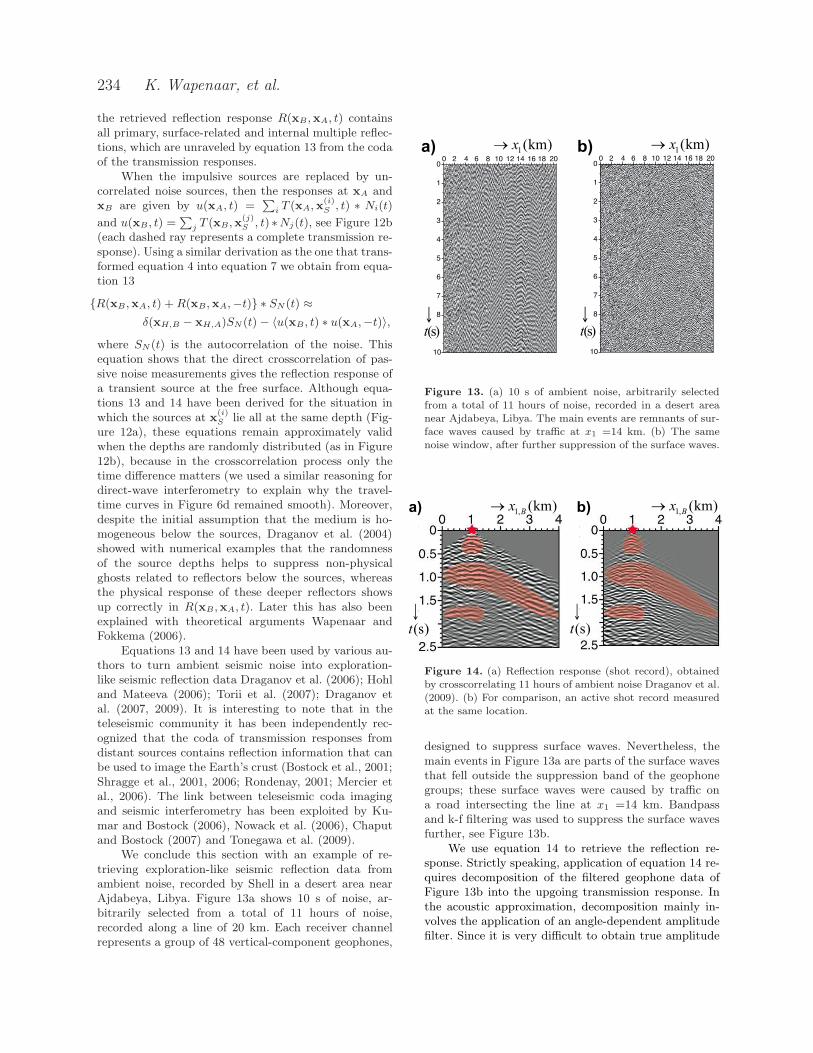
We conclude this section with an example of re-trieving exploration-like seismic reflection data fromambient noise, recorded by Shell in a desert area nearAjdabeya, Libya. Figure 13a shows 10 s of noise, ar-bitrarily selected from a total of 11 hours of noise,recorded along a line of 20 km. Each receiver channelrepresents a group of 48 vertical-component geophones,

0

1

2

3

4

5

6

7

8

9

10

Horizontal distance (km)

Re

lative

tra

ve

ltim

e (

s)

0 2 4 6 8 10 12 14 16 18 200

1

2

3

4

5

6

7

8

9

10

Re

lative

tra

ve

ltim

e (

s)

0Horizontal distance (km)2 4 6 8 10 12 14 16 18 20

a) b) 1(km)x 1(km)x

(s)t(s)t

Figure 13. (a) 10 s of ambient noise, arbitrarily selectedfrom a total of 11 hours of noise, recorded in a desert areanear Ajdabeya, Libya. The main events are remnants of sur-face waves caused by traffic at x1 =14 km. (b) The samenoise window, after further suppression of the surface waves.

a) b)1, (km)Bx 1, (km)B

x

(s)t (s)t

Figure 14. (a) Reflection response (shot record), obtainedby crosscorrelating 11 hours of ambient noise Draganov et al.(2009). (b) For comparison, an active shot record measuredat the same location.

designed to suppress surface waves. Nevertheless, themain events in Figure 13a are parts of the surface wavesthat fell outside the suppression band of the geophonegroups; these surface waves were caused by traffic ona road intersecting the line at x1 =14 km. Bandpassand k-f filtering was used to suppress the surface wavesfurther, see Figure 13b.

We use equation 14 to retrieve the reflection re-sponse. Strictly speaking, application of equation 14 re-quires decomposition of the filtered geophone data ofFigure 13b into the upgoing transmission response. Inthe acoustic approximation, decomposition mainly in-volves the application of an angle-dependent amplitudefilter. Since it is very difficult to obtain true amplitude


responses from ambient noise anyway, the decomposi-tion step is skipped. Using equation 14, with xA fixed(x1,A = 1 km) and xB chosen variable (x1,B = 0 · · · 4km), a seismic shot record R(xB,xA, t) is retrieved fromthe noise, of which the first 2.5 s are shown in Figure14a. The red star at x1,B = x1,A = 1 km denotes the po-sition of the virtual source. An active seismic reflectionexperiment, carried out with the source at the same po-sition, is shown in Figure 14b. Note that, particularly inthe red shaded areas, the reflections retrieved from theambient noise (Figure 14a) correspond quite well withthose in the active shot gather (Figure 14b). For moredetails about this experiment as well as a pseudo 3Dreflection image obtained from the ambient noise, seeDraganov et al. (2009).

CONCLUSIONS

We have discussed the basic principles of seismic in-terferometry in a heuristic way. We have shown that,whether we consider controlled-source or passive inter-ferometry, virtual sources are created at positions wherethere are only receivers. Of course no new informationis generated by interferometry, but information hiddenin noise or in a complex scattering coda, is reorganizedinto easy interpretable responses that can be furtherprocessed by standard tomographic inversion or reflec-tion imaging methodologies. The main strength is thatthis “information unraveling” neither requires knowl-edge of the subsurface medium parameters nor of thepositions or timing of the actual sources. Moreover, theprocessing consists of simple crosscorrelations and is al-most entirely data-driven.

In Part II we discuss the relation between inter-ferometry and time-reversed acoustics, review a mathe-matically sound derivation, and indicate recent and newadvances.

ACKNOWLEDGEMENTS

This work is supported by the Netherlands ResearchCentre for Integrated Solid Earth Science (ISES), theDutch Technology Foundation STW, applied sciencedivision of NWO and the Technology Program of theMinistry of Economic Affairs (grant VENI.08115), andby the NSF through grant EAS-0609595. We thank as-sociate editor Sven Treitel and reviewers Jerry Schus-ter, Kasper van Wijk and Mark Willis for their valu-able comments and suggestions, which helped improvethis paper. We are grateful to Fan-Chi Lin, Mike Ritz-woller and Wiley-Blackwell (publisher of GeophysicalJournal International) for permission to show the snap-shots of the virtual Rayleigh-wave response (Figure 7).Jerry Schuster is acknowledged for providing Figure 11.Last, but not least, we thank the Libyan National OilCompany for permission to publish the Ajdabeya data

ray A

ray BiB i

A

q1

FIG. A-1 Two rays, A and B, that propagate from a commonpoint on the surface with sources (dashed line) and theirtake-off angles at this source surface.

results (Figures 13 and 14) and Shell in Libya for col-lecting and making available the passive data.

APPENDIX A: STATIONARY-PHASE

ANALYSIS

We give a simple proof that the stationary point of thetraveltime curve in a correlation gather corresponds tothe source from which the rays to the receivers at xA

and xB leave in the same direction. Consider two raysA and B that propagate from an arbitrary source pointto the two receivers, see Figure A-1. This propagationmay be direct, or it may involve bounces off reflectorsor scatterers; the fate of these rays is irrelevant for theargument presented here. The sources involved in inter-ferometry are located on the surface indicated by thedashed line in Figure A-1. This surface, which need notbe planar, is in 3D parameterized by two orthogonal co-ordinates q1 and q2. We first keep q2 fixed and consideronly variations in q1.

The travel time from a given source to the receiverat xA is denoted by tA, and the travel time from thatsource to the receiver at xB by tB . These travel timesare, in general, functions of the source position q1. Inseismic interferometry, the traveltimes of the signalsthat are crosscorrelated are subtracted. This means thatthe traveltime tcorr of the crosscorrelation for a givensource position is given by

tcorr(q1) = tB(q1) − tA(q1). (A1)

The condition that the traveltime is stationary meansthat

∂tcorr(q1)

∂q1=

∂tB(q1)

∂q1− ∂tA(q1)

∂q1= 0. (A2)


A standard derivation Aki and Richards (1980) relatesthe slowness along the surface to the take-off angle

∂tA(q1)

∂q1=

sin iAc

, (A3)

with c the propagation velocity. A similar expressionholds for tB. Inserting this in equation (A-2) impliesthat at the stationary point

iA = iB . (A4)

This means that at the stationary source point the raystake off in the same direction.

The reasoning above was applicable to variationsin the source coordinate q1. The same reasoning appliesto variations with the orthogonal source coordinate q2.This means that the rays take off in the same directionas measured in two orthogonal planes, hence, the rayshave the same direction in three dimensions. Therefore,the rays radiating from the stationary source positionare parallel.

References

Aki, K. and P. G. Richards, 1980, Quantitative seismol-ogy, Vol. I: W.H. Freeman and Company, San Fran-sisco.

Aki, K., 1957, Space and time spectra of stationarystochastic waves, with special reference to micro-tremors: Bulletin of the Earthquake Research Insti-tute, 35, 415–457.

Aki, K., 1965, A note on the use of microseisms in de-termining the shallow structures of the earth’s crust:Geophysics, 30, 665–666.

Asten, M. W., 2006, On bias and noise in passive seis-mic data from finite circular array data processed us-ing SPAC methods: Geophysics, 71, V153–V162.

Bakulin, A. and R. Calvert, 2004, Virtual source: newmethod for imaging and 4D below complex overbur-den: 74th Annual International Meeting, SEG, Ex-panded Abstracts, 2477–2480.

Bakulin, A. and R. Calvert, 2006, The virtual sourcemethod: Theory and case study: Geophysics, 71,SI139–SI150.

Baskir, E. and C. E. Weller, 1975, Sourceless reflectionseismic exploration (abstract of paper presented atthe 44th Annual International SEG Meeting): Geo-physics, 40, 158–159.

Bensen, G. D., M. H. Ritzwoller, M. P. Barmin, A. L.Levshin, F. Lin, M. P. Moschetti, N. M. Shapiro,and Y. Yang, 2007, Processing seismic ambient noisedata to obtain reliable broad-band surface wave dis-persion measurements: Geophysical Journal Interna-tional, 169, 1239–1260.

Bensen, G. D., M. H. Ritzwoller, and N. M. Shapiro,2008, Broadband ambient noise surface wave tomog-raphy across the United States: Journal of Geophys-

ical Research - Solid Earth, 113, B05306–1–B05306–21.

Berryhill, J. R., 1979, Wave-equation datuming: Geo-physics, 44, 1329–1344.

Berryhill, J. R., 1984, Wave-equation datuming beforestack: Geophysics, 49, 2064–2066.

Bostock, M. G., S. Rondenay, and J. Shragge, 2001,Multiparameter two-dimensional inversion of scat-tered teleseismic body waves. 1. Theory for obliqueincidence: Journal of Geophysical Research, 106,30771–30782.

Brenguier, F., N. M. Shapiro, M. Campillo, A. Nerces-sian, and V. Ferrazzini, 2007, 3-D surface wave tomog-raphy of the Piton de la Fournaise volcano using seis-mic correlations: Geophysical Research Letters, 34,L02305–1–L02305–5.

Brooks, L. A. and P. Gerstoft, 2007, Ocean acousticinterferometry: Journal of the Acoustical Society ofAmerica, 121, no. 6, 3377–3385.

Callen, H. B. and T. A. Welton, 1951, Irreversibilityand generalized noise: Physical Review, 83, 34–40.

Campillo, M. and A. Paul, 2003, Long-range correla-tions in the diffuse seismic coda: Science, 299, 547–549.

Challis, L. and F. Sheard, 2003, The Green of Greenfunctions: Physics Today, 56, 41–46.

Chapman, C. H., 1994, Reflection/transmission coeffi-cients reciprocities in anisotropic media: GeophysicalJournal International, 116, 498–501.

Chaput, J. A. and M. G. Bostock, 2007, Seismic in-terferometry using non-volcanic tremor in Cascadia:Geophysical Research Letters, 34, L07304–1–L07304–5.

Claerbout, J. F., 1968, Synthesis of a layered mediumfrom its acoustic transmission response: Geophysics,33, 264–269.

Cole, S., 1995, Passive seismic and drill-bit experi-ments using 2-D arrays: Ph.D. thesis, Stanford Uni-versity.

Curtis, A., P. Gerstoft, H. Sato, R. Snieder, andK. Wapenaar, 2006, Seismic interferometry - turn-ing noise into signal: The Leading Edge, 25, no. 9,1082–1092.

Daneshvar, M. R., C. S. Clay, and M. K. Savage, 1995,Passive seismic imaging using microearthquakes: Geo-physics, 60, 1178–1186.

de Hoop, A. T., 1988, Time-domain reciprocity the-orems for acoustic wave fields in fluids with relax-ation: Journal of the Acoustical Society of America,84, 1877–1882.

Dong, S., R. He, and G. T. Schuster, 2006a, Interfero-metric prediction and least squares subtraction of sur-face waves: 76th Annual International Meeting, SEG,Expanded Abstracts, 2783–2786.

Dong, S., J. Sheng, and G. T. Schuster, 2006b, The-ory and practice of refraction interferometry: 76thAnnual International Meeting, SEG, Expanded Ab-


stracts, 3021–3025.Draganov, D., K. Wapenaar, and J. Thorbecke, 2004,Passive seismic imaging in the presence of white noisesources: The Leading Edge, 23, no. 9, 889–892.

Draganov, D., K. Wapenaar, W. Mulder, and J. Singer,2006, Seismic interferometry on background-noisefield data: 76th Annual International Meeting, SEG,Expanded Abstracts, 590–593.

Draganov, D., K. Wapenaar, W. Mulder, J. Singer,and A. Verdel, 2007, Retrieval of reflections fromseismic background-noise measurements: GeophysicalResearch Letters, 34, L04305–1–L04305–4.

Draganov, D., X. Campman, J. Thorbecke, A. Verdel,and K. Wapenaar, 2009, Reflection images from am-bient seismic noise: Geophysics, 74, A63–A67.

Duvall, T. L., S. M. Jefferies, J. W. Harvey, and M. A.Pomerantz, 1993, Time-distance helioseismology: Na-ture, 362, 430–432.

Fan, Y. and R. Snieder, 2009, Required source distri-bution for interferometry of waves and diffusive fields:Geophysical Journal International, 179, 1232–1244.

Fokkema, J. T. and P. M. van den Berg, 1993, Seismicapplications of acoustic reciprocity: Elsevier, Amster-dam.

Frasier, C. W., 1970, Discrete time solution of planeP-SV waves in a plane layered medium: Geophysics,35, 197–219.

Gerstoft, P., K. G. Sabra, P. Roux, W. A. Kuperman,and M. C. Fehler, 2006, Green’s functions extrac-tion and surface-wave tomography from microseismsin southern California: Geophysics, 71, SI23–SI31.

Godin, O. A., 2007, Emergence of the acoustic Green’sfunction from thermal noise: Journal of the AcousticalSociety of America, 121, no. 2, EL96–EL102.

Gouedard, P., P. Roux, M. Campillo, and A. Verdel,2008a, Convergence of the two-point correlation func-tion toward the Green’s function in the context of aseismic-prospecting data set: Geophysics, 73, V47–V53.

Gouedard, P., L. Stehly, F. Brenguier, M. Campillo,Y. Colin de Verdiere, E. Larose, L. Margerin, P. Roux,F. J. Sanchez-Sesma, N. M. Shapiro, and R. L.Weaver, 2008b, Cross-correlation of random fields:mathematical approach and applications: Geophysi-cal Prospecting, 56, 375–393.

Green, G., 1828, An essay on the application of mathe-matical analysis to the theories of electricity and mag-netism: Privately published.

Halliday, D. F., A. Curtis, J. O. A. Robertsson, andD.-J. van Manen, 2007, Interferometric surface-waveisolation and removal: Geophysics, 72, A69–A73.

Halliday, D., A. Curtis, P. Vermeer, C. L. Strobbia,A. Glushchenko, D.-J. van Manen, and J. Robertsson,2010, Interferometric ground-roll removal: Attenua-tion of scattered surface waves in single-sensor data:Geophysics, 75, (accepted).

Haskell, N. A., 1953, The dispersion of surface waves

on multilayered media: Bulletin of the SeismologicalSociety of America, 43, 17–34.

He, R., B. Hornby, and G. Schuster, 2007, 3Dwave-equation interferometric migration of VSP free-surface multiples: Geophysics, 72, S195–S203.

Henstridge, J. D., 1979, A signal processing methodfor circular arrays: Geophysics, 44, 179–184.

Hohl, D. and A. Mateeva, 2006, Passive seismic reflec-tivity imaging with ocean-bottom cable data: 76thAnnual International Meeting, SEG, Expanded Ab-stracts, 1560–1563.

Hornby, B. E. and J. Yu, 2007, Interferometric imagingof a salt flank using walkaway VSP data: The LeadingEdge, 26, no. 6, 760–763.

Jiang, Z., J. Sheng, J. Yu, G. T. Schuster, andB. E. Hornby, 2007, Migration methods for imag-ing different-order multiples: Geophysical Prospect-ing, 55, 1–19.

Kang, T.-S. and J. S. Shin, 2006, Surface-wave tomog-raphy from ambient seismic noise of accelerographnetworks in southern Korea: Geophysical ResearchLetters, 33, L17303–1–L17303–5.

Kennett, B. L. N., N. J. Kerry, and J. H. Woodhouse,1978, Symmetries in the reflection and transmissionof elastic waves: Geophysical Journal of the Royal As-tronomical Society, 52, 215–230.

Kumar, M. R. and M. G. Bostock, 2006, Transmissionto reflection transformation of teleseismic wavefields:Journal of Geophysical Research - Solid Earth, 111,B08306–1–B08306–9.

Larose, E., A. Khan, Y. Nakamura, and M. Campillo,2005, Lunar subsurface investigated from correlationof seismic noise: Geophysical Research Letters, 32,L16201–1–L16201–4.

Larose, E., L. Margerin, A. Derode, B. van Tiggelen,M. Campillo, N. Shapiro, A. Paul, L. Stehly, andM. Tanter, 2006, Correlation of random wave fields:An interdisciplinary review: Geophysics, 71, SI11–SI21.

Le Bellac, M., F. Mortessagne, and G. G. Ba-trouni, 2004, Equilibrium and non-equilibrium statis-tical thermodynamics: Cambridge Univ. Press, Cam-bridge, UK.

Li, H., W. Su, C.-Y. Wang, and Z. Huang, 2009, Am-bient noise Rayleigh wave tomography in westernSichuan and eastern Tibet: Earth and Planetary Sci-ence Letters, 282, 201–211.

Liang, C. and C. A. Langston, 2008, Ambient seis-mic noise tomography and structure of eastern NorthAmerica: Journal of Geophysical Research - SolidEarth, 113, B03309–1–B03309–18.

Lin, F.-C., M. P. Moschetti, and M. H. Ritzwoller,2008, Surface wave tomography of the western UnitedStates from ambient seismic noise: Rayleigh and Lovewave phase velocity maps: Geophysical Journal Inter-national, 173, 281–298.

Lin, F.-C., M. H. Ritzwoller, and R. Snieder, 2009,


Eikonal tomography: surface wave tomography byphase front tracking across a regional broad-bandseismic array: Geophysical Journal International,177, 1091–1110.

Lobkis, O. I. and R. L. Weaver, 2001, On the emergenceof the Green’s function in the correlations of a diffusefield: Journal of the Acoustical Society of America,110, 3011–3017.

Longuet-Higgins, M. S., 1950, A theory for the genera-tion of microseisms: Philosophical Transactions of theRoyal Society of London. Series A, 243, 1–35.

Lu, R., M. Willis, X. Campman, and T. M. N. Ajo-Franklin, J., 2008, Redatuming through a salt canopyand target-oriented salt-flank imaging: Geophysics,73, S63–S71.

Ma, S., G. A. Prieto, and G. C. Beroza, 2008, Testingcommunity velocity models for Southern Californiausing the ambient seismic field: Bulletin of the Seis-mological Society of America, 98, 2694–2714.

Malcolm, A. E., J. A. Scales, and B. A. van Tigge-len, 2004, Extracting the Green function from dif-fuse, equipartitioned waves: Physical Review E, 70,015601(R)–1–015601(R)–4.

Mercier, J.-P., M. G. Bostock, and A. M. Baig, 2006,Improved green’s functions for passive-source struc-tural studies: Geophysics, 71, SI95–SI102.

Mikesell, D., K. van Wijk, A. Calvert, and M. Haney,2009, The virtual refraction: Useful spurious energyin seismic interferometry: Geophysics, 74, A13–A17.

Minato, S., K. Onishi, T. Matsuoka, Y. Oka-jima, J. Tsuchiyama, D. Nobuoka, H. Azuma, andT. Iwamoto, 2007, Cross-well seismic survey withoutborehole source: 77th Annual International Meeting,SEG, Expanded Abstracts, 1357–1361.

Miyazawa, M., R. Snieder, and A. Venkataraman,2008, Application of seismic interferometry to extractP- and S-wave propagation and observation of shear-wave splitting from noise data at Cold Lake, Alberta,Canada: Geophysics, 73, D35–D40.

Nowack, R. L., S. Dasgupta, G. T. Schuster, and J.-M.Sheng, 2006, Correlation migration using Gaussianbeams of scattered teleseismic body waves: Bulletinof the Seismological Society of America, 96, 1–10.

Okada, H., 2003, The microtremor survey method: So-ciety of Exploration Geophysicists.

Okada, H., 2006, Theory of efficient array observationsof microtremors with special reference to the SPACmethod: Exploration Geophysics, 37, 73–85.

Perton, M., F. J. Sanchez-Sesma, A. Rodrıguez-Castellanos, M. Campillo, and R. L. Weaver, 2009,Two perspectives on equipartition in diffuse elasticfields in three dimensions: Journal of the AcousticalSociety of America, 126, 1125–1130.

Picozzi, M., S. Parolai, D. Bindi, and A. Strollo,2009, Characterization of shallow geology by high-frequency seismic noise tomography: GeophysicalJournal International, 176, 164–174.

Poletto, F. and L. Petronio, 2003, Transmitted andreflected waves in tunnel SWD: 73rd Annual Inter-national Meeting, SEG, Expanded Abstracts, 1211–1214.

Poletto, F. and L. Petronio, 2006, Seismic interferom-etry with a TBM source of transmitted and reflectedwaves: Geophysics, 71, SI85–SI93.

Ramırez, A. C. and A. B. Weglein, 2009, Green’s theo-rem as a comprehensive framework for data recon-struction, regularization, wavefield separation, seis-mic interferometry, and wavelet estimation: A tuto-rial: Geophysics, 74, W35–W62.

Rickett, J. and J. Claerbout, 1999, Acoustic daylightimaging via spectral factorization: Helioseismologyand reservoir monitoring: The Leading Edge, 18, no.8, 957–960.

Rondenay, S., M. G. Bostock, and J. Shragge, 2001,Multiparameter two-dimensional inversion of scat-tered teleseismic body waves. 3. Application to theCascadia 1993 data set: Journal of Geophysical Re-search, 106, 30795–30807.

Roux, P. and M. Fink, 2003, Green’s function estima-tion using secondary sources in a shallow water envi-ronment: Journal of the Acoustical Society of Amer-ica, 113, no. 3, 1406–1416.

Rytov, S. M., Y. A. Kravtsov, and V. I. Tatarskii, 1989,Principles of statistical radiophysics. 3: Elements ofrandom fields: Springer, Berlin.

Rytov, S. M., 1956, On thermal fluctuations in dis-tributed systems: Doklady Akademii nauk SSSR,110, 371.

Sabra, K. G., P. Gerstoft, P. Roux, W. A. Kuper-man, and M. C. Fehler, 2005a, Extracting time-domain Green’s function estimates from ambient seis-mic noise: Geophysical Research Letters, 32, L03310–1–L03310–5.

——– 2005b, Surface wave tomography from micro-seisms in Southern California: Geophysical ResearchLetters, 32, L14311–1–L14311–4.

Sabra, K. G., P. Roux, and W. A. Kuperman, 2005c,Arrival-time structure of the time-averaged ambientnoise cross-correlation function in an oceanic waveg-uide: Journal of the Acoustical Society of America,117, no. 1, 164–174.

Sanchez-Sesma, F. J., J. A. Perez-Ruiz, M. Campillo,and F. Luzon, 2006, Elastodynamic 2D Green func-tion retrieval from cross-correlation: Canonical in-clusion problem: Geophysical Research Letters, 33,L13305–1–L13305–6.

Scherbaum, F., 1987a, Seismic imaging of the siteresponse using microearthquake recordings. Part I.Method: Bulletin of the Seismological Society ofAmerica, 77, 1905–1923.

——– 1987b, Seismic imaging of the site response usingmicroearthquake recordings. Part II. Application tothe Swabian Jura, Southwest Germany, seismic net-work: Bulletin of the Seismological Society of Amer-


ica, 77, 1924–1944.Schuster, G. T. and M. Zhou, 2006, A theoreticaloverview of model-based and correlation-based reda-tuming methods: Geophysics, 71, SI103–SI110.

Schuster, G. T., J. Yu, J. Sheng, and J. Rickett, 2004,Interferometric/daylight seismic imaging: Geophysi-cal Journal International, 157, 838–852.

Schuster, G. T., 2001, Theory of day-light/interferometric imaging: tutorial: 63rd AnnualInternational Meeting, EAGE, Extended Abstracts,Session: A32.

Schuster, G. T., 2009, Seismic interferometry: Cam-bridge University Press.

Shapiro, N. M. and M. Campillo, 2004, Emergence ofbroadband Rayleigh waves from correlations of theambient seismic noise: Geophysical Research Letters,31, L07614–1–L07614–4.

Shapiro, N. M., M. Campillo, L. Stehly, and M. H.Ritzwoller, 2005, High-resolution surface-wave to-mography from ambient seismic noise: Science, 307,1615–1618.

Shragge, J., M. G. Bostock, and S. Rondenay, 2001,Multiparameter two-dimensional inversion of scat-tered teleseismic body waves. 2. Numerical examples:Journal of Geophysical Research, 106, 30783–30793.

Shragge, J., B. Artman, and C. Wilson, 2006, Tele-seismic shot-profile migration: Geophysics, 71, SI221–SI229.

Snieder, R., K. Wapenaar, and U. Wegler, 2007, Uni-fied Green’s function retrieval by cross-correlation;connection with energy principles: Physical ReviewE, 75, 036103–1–036103–14.

Snieder, R., 2004, Extracting the Green’s function fromthe correlation of coda waves: A derivation based onstationary phase: Physical Review E, 69, 046610–1–046610–8.

Stehly, L., M. Campillo, and N. M. Shapiro, 2006, Astudy of the seismic noise from its long-range cor-relation properties: Journal of Geophysical Research,111, B10306–1–B10306–12.

Thompson, A. R., J. M. Moran, and G. W. Swen-son Jr., 2001, Interferometry and synthesis in radioastronomy: Wiley-Interscience, New York.

Thomson, W. T., 1950, Transmission of elastic wavesthrough a stratified solid medium: Journal of AppliedPhysics, 21, 89–93.

Toksoz, M. N., 1964, Microseisms and an attemptedapplication to exploration: Geophysics, 39, 154–177.

Tonegawa, T., K. Nishida, T. Watanabe, and K. Sh-iomi, 2009, Seismic interferometry of teleseismic S-wave coda for retrieval of body waves: an applicationto the Philippine Sea slab underneath the Japanese Is-lands: Geophysical Journal International, 178, 1574–1586.

Torii, K., T. Matsuoka, K. Onishi, K. Shirashi,T. Aizawa, Y. Yamanaka, S. Ito, T. Kimura,Y. Asano, and T. Takeda, 2007, Application of seis-

mic interferometry to natural earthquakes measuredby small-scale array: 77th Annual International Meet-ing, SEG, Expanded Abstracts, 1362–1366.

Ursin, B., 1983, Review of elastic and electromagneticwave propagation in horizontally layered media: Geo-physics, 48, 1063–1081.

van Tiggelen, B. A., 2003, Green function retrieval andtime reversal in a disordered world: Physical ReviewLetters, 91, 243904–1–243904–4.

Wang, Y., Y. Luo, and G. T. Schuster, 2009, Inter-ferometric interpolation of missing seismic data: Geo-physics, 74, SI37–SI45.

Wapenaar, K. and J. Fokkema, 2006, Green’s func-tion representations for seismic interferometry: Geo-physics, 71, SI33–SI46.

Wapenaar, C. P. A. and J. L. T. Grimbergen, 1996,Reciprocity theorems for one-way wave fields: Geo-physical Journal International, 127, 169–177.

Wapenaar, K., D. Draganov, J. Thorbecke, andJ. Fokkema, 2002, Theory of acoustic daylight imag-ing revisited: 72nd Annual International Meeting,SEG, Expanded Abstracts, 2269–2272.

Wapenaar, K., J. Thorbecke, and D. Draganov, 2004,Relations between reflection and transmission re-sponses of three-dimensional inhomogeneous media:Geophysical Journal International, 156, 179–194.

Weaver, R. L. and O. I. Lobkis, 2001, Ultrasonics with-out a source: Thermal fluctuation correlations at MHzfrequencies: Physical Review Letters, 87, 134301–1–134301–4.

Weaver, R. L. and O. I. Lobkis, 2002, On the emergenceof the Green’s function in the correlations of a diffusefield: pulse-echo using thermal phonons: Ultrasonics,40, 435–439.

Weaver, R., B. Froment, and M. Campillo, 2009, Onthe correlation of non-isotropically distributed ballis-tic scalar diffuse waves: Journal of the Acoustical So-ciety of America, 126, 1817–1826.

Webb, S. C., 1998, Broadband seismology and noiseunder the ocean: Reviews of Geophysics, 36, 105–142.

Willis, M. E., R. Lu, X. Campman, M. N. Toksoz,Y. Zhang, and M. V. de Hoop, 2006, A novel applica-tion of time-reversed acoustics: Salt-dome flank imag-ing using walkaway VSP surveys: Geophysics, 71, A7–A11.

Xiao, X., M. Zhou, and G. T. Schuster, 2006, Salt-flankdelineation by interferometric imaging of transmittedP- and S-waves: Geophysics, 71, SI197–SI207.

Xue, Y., S. Dong, and G. T. Schuster, 2009, Interfer-ometric prediction and subtraction of surface waveswith a nonlinear local filter: Geophysics, 74, SI1–SI8.

Yao, H., R. D. van der Hilst, and M. V. de Hoop,2006, Surface-wave array tomography in SE Tibetfrom ambient seismic noise and two-station analysis -I. Phase velocity maps: Geophysical Journal Interna-tional, 166, 732–744.

Yao, H., C. Beghein, and R. D. van der Hilst, 2008,


Surface-wave array tomography in SE Tibet fromambient seismic noise and two-station analysis -II. Crustal and upper-mantle structure: GeophysicalJournal International, 173, 205–219.

Yao, H., X. Campman, M. V. de Hoop, and R. D.van der Hilst, 2009, Estimation of surface waveGreen’s functions from correlation of direct waves,coda waves, and ambient noise in SE Tibet: Physicsof the Earth and Planetary Interiors, 177, 1–11.

Yokoi, T. and S. Margaryan, 2008, Consistency of thespatial autocorrelation method with seismic interfer-ometry and its consequence: Geophysical Prospect-ing, 56, 435–451.

Yu, J. and G. T. Schuster, 2006, Crosscorrelogram mi-gration of inverse vertical seismic profile data: Geo-physics, 71, S1–S11.

cwp-658

Documents

source seismic interferometry

term seismic interferometry

passive seismic interferometry

seismic interferometry

basic principles of

wave phenomena

plane wave

seismic reflection response