cyclic behavior and dynamic properties of soils: a case of
TRANSCRIPT
CYCLIC BEHAVIOUR AND DYNAMIC PROPERTIES
OF SOILS: A CASE OF JIMMA TOWN
TESHOME BIRHANU KEBEDE
MASTER OF SCIENCE
ADDIS ABABA SCIENCE AND TECHNOLOGY
UNIVERSITY
JANUARY 2019
CYCLIC BEHAVIOUR AND DYNAMIC PROPERTIES OF SOILS: A
CASE OF JIMMA TOWN
By
TESHOME BIRHANU KEBEDE
A Thesis Submitted to the Department of Civil Engineering for the Partial Fulfillment of
the Requirements for the Degree of Master of Science in Civil Engineering
(Geotechnical Engineering)
ADDIS ABABA SCIENCE AND TECHNOLOGY UNIVERSITY
JANUARY 2019
i
Declaration
I hereby declare that this thesis entitled “CYCLIC BEHAVIOUR AND DYNAMIC
PROPERTIES OF SOILS: A CASE OF JIMMA TOWN” was composed by myself,
with the guidance of my advisor, that the work contained herein is my own except where
explicitly stated otherwise in the text, and that this work has not been submitted, in whole
or in part, for any other degree or professional qualification.
Name: Signature, Date:
ii
Certificate
This is to certify that the thesis prepared by Mr. Teshome Birhanu Kebede entitled
“Cyclic Behaviour and Dynamic Properties Of Soils: A Case of Jimma Town” and
submitted in fulfillment of the requirements for the Degree of Master of Science complies
with the regulations of the University and meets the accepted standards with respect to
originality and quality.
Singed by Examining Board:
Examiner: Signature, Date:
Examiner: Signature, Date:
Thesis Advisor: Signature, Date:
Thesis Co-Advisor: Signature, Date:
iii
Abstract
The objective of the research is to investigate the dynamic properties of typical soils
found in Jimma town. To meet its objective samples from different parts of the city were
collected and laboratory tests were done on the collected samples. From the index
property test silty and clayey soils dominate the area, having the liquid limit value
ranging from 67% to 84% and plasticity index value of 31% to 46%. The specific gravity
value ranges from 2.53 to 2.72. Cyclic simple shear test were conducted at cyclic shear
strain of 0.01%, 0.1%, 1%, 2.5% and 5% under axial stress of 100 kPa, 250 kPa and 400
kPa. The value of shear modules found in the laboratory ranges from 0.33 to 7.01 MPa
and damping ratio values from 2.03 to 22.98%. The shear modulus values were used to
calculate the normalized shear modulus (G/Gmax) value which is used for comparison
with previous studies. The results have shown that the obtained (G/Gmax) values have
good agreement with curve developed by previous researchers but at lower strains the
obtained result was lower. For higher strains the obtained (G/Gmax) values agree with
those suggested in literature. This shows that testing conditions, sample preparation and
type of soil sample have significant effect on the shear modulus values and damping
characteristics, especially at small strain levels.
Key words: - Cyclic simple shear test, Damping ratio, Dynamic properties, Normalized
shear modulus, Shear modulus and shear strain.
.

iv
Acknowledgements
I am thankful to God as He has been grateful to me much more than I deserve and to my
all teachers from school level to university level. Besides, I would like to thank my Dad,
Mom and Sister for being by my side in every challenges and difficulties I faced.
I’m also greatly indebted to the people and institution that made the writing of this
project successful. Special thanks go to my supervisor, Dr. Yoseph Birru for his
invaluable guidance, continuous assistance and encouragement throughout the writing of
this thesis.
v
Table of Contents
Declaration ........................................................................................................................... i
Certificate ............................................................................................................................ ii
Approval page .................................................................................................................... iii
Acknowledgements ............................................................................................................ iv
LIST OF TABLES ........................................................................................................... viii
LIST OF FIGURES ........................................................................................................... ix
ABBREVIATIONS .......................................................................................................... xii
CHAPTER ONE ................................................................................................................. 1
INTRODUCTION ..................................................................................... 1
1.1 Background ...................................................................................... 1
1.2 Objective of the study ...................................................................... 2
1.3 Methodology .................................................................................... 2
1.4 Scope and limitation of the study .................................................... 3
1.5 Organization of the thesis ................................................................ 3
CHAPTER TWO ................................................................................................................ 4
LITERATURE REVIEW ............................................................................. 4
2.1 Introduction ...................................................................................... 4
2.2 Dynamic soil properties ................................................................... 5
2.3 Methods of Determining Shear Modules and Damping
Characteristics ........................................................................................... 8
2.4 Parameters Affecting dynamic soil properties ...............................11
CHAPTER THREE .......................................................................................................... 24
DESCRIPTION OF STUDY AREA ..........................................................24
3.1 Geology ..........................................................................................25
CHAPTER FOUR ............................................................................................................. 27
EXPERIMENTAL PROGRAMME ...........................................................27
vi
4.1. Overview of testing equipment ......................................................27
4.2 Field and laboratory tests ...............................................................28
4.2.1 One-dimensional Consolidation .................................................30
4.2.2 Simple cyclic shear test procedures ............................................30
4.2.3 Presentation of Cyclic Shear Test results ...................................33
4.2.4 Computation of shear modulus and damping ratio values .........36
CHAPTER FIVE .............................................................................................................. 44
RESULT AND DISCUSSIONS .............................................................44
5.1 Dependency of shear modulus and damping ratio on shear strain
amplitude .................................................................................................44
5.2 Influence of effective vertical stress on Shear Modulus and
damping ratio ...........................................................................................45
5.3 Influence of number of loading cycles on shear modulus and
damping ratio ...........................................................................................46
5.4 Effect of void ratio on damping ratio ............................................47
5.5 Effect of soil plasticity on damping ratio and shear modulus .......48
5.6 Determination of maximum shear modulus ..................................49
CHAPTER SIX ................................................................................................................. 56
CONCLUSIONS AND RECOMMENDATIONS .................................56
REFERENCES ................................................................................................................. 58

vii
APPENDIX A ................................................................................................................... 60
Atterberg limit test results ..........................................................................60
Preparation and assembling of test specimens ...........................................66
APPENDIX: B .................................................................................................................. 67
Consolidation test results ............................................................................67
APPENDIX C ................................................................................................................... 71
Cyclic shear test result ................................................................................71
C.2 Shear modulus and damping ratio values of selected cycles ...............83
APPENDIX D ................................................................................................................... 87
Shear modulus and Damping ratio curves which show dependency on
different factors...........................................................................................87
viii
LIST OF TABLES
Table 2. 1: Value of a with respect to plasticity index (Hardin, 1972) ............................... 8
Table 2. 2: Test procedures for measuring moduli and damping characteristics (Seed &
Idriss, 1970) ...................................................................................................................... 10
Table 4. 1: Atterberg limits and soil classification ........................................................... 29
Table 4. 2: Axial stress and shear strain values used for the study ................................... 33
Table 4. 3: Shear stress and shear strain values for single cycle. ..................................... 35
Table 4. 4: Typical tabulation for shear stress and shear strain values ............................. 38
Table 4. 5: Typical calculation for shear modulus and damping ratio using table 4.3 and
figure 4.8 ........................................................................................................................... 41
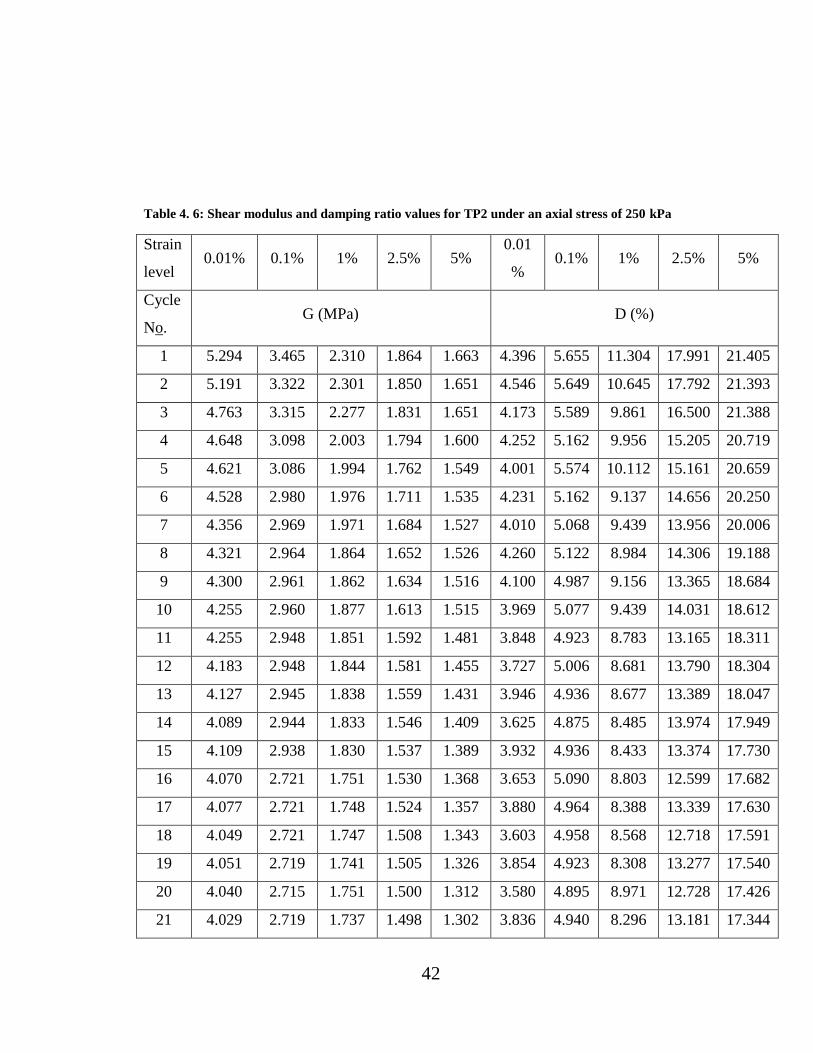
Table 4. 6: Shear modulus and damping ratio values for TP2 under an axial stress of 250
kPa..................................................................................................................................... 42
Table 5. 1: maximum shear modulus determination at different axial stress ................... 50
Table 5. 2: Normalized shear modulus (G/Gmax) versus shearing strain amplitude ....... 51
Table A- 1: Determination of Liquid Limit, Plastic Limit and Plastic Index (for TP1) ... 63
Table A- 2: Determination of Liquid Limit, Plastic Limit and Plastic Index (for TP2) ... 64
Table A- 3: Determination of Liquid Limit, Plastic Limit and Plastic Index (for TP3) ... 63
Table A- 4: Determination of Liquid Limit, Plastic Limit and Plastic Index (for TP4) ... 64
Table B- 1: Determination of Pre-consolidation pressure for TP1 ................................... 67
Table B- 2: Determination of Pre-consolidation pressure for TP2 ................................... 69
Table C- 1: Shear modulus and damping ratio values for TP1 at 100 kPa ....................... 83
Table C- 2: Shear modulus and damping ratio values for TP1 at 400 kPa ....................... 84
Table C- 3: Shear modulus and damping ratio values for TP2 at 100 kPa ....................... 85
Table C- 4: Shear modulus and damping ratio values for TP2 at 250 kPa ....................... 86
ix
LIST OF FIGURES
Figure 2. 1: Hysteresis loop for one cycle of loading showing Gmax, G, and D (Seed &
Idriss, 1970) ........................................................................................................................ 6
Figure 2. 2: Hypothetical Particle Structure of Loose Silty Sand with Low Silt Content (a)
As Deposited and (b) After Densification due to Shearing. (Yamamuro & Lade, 1999) . 13
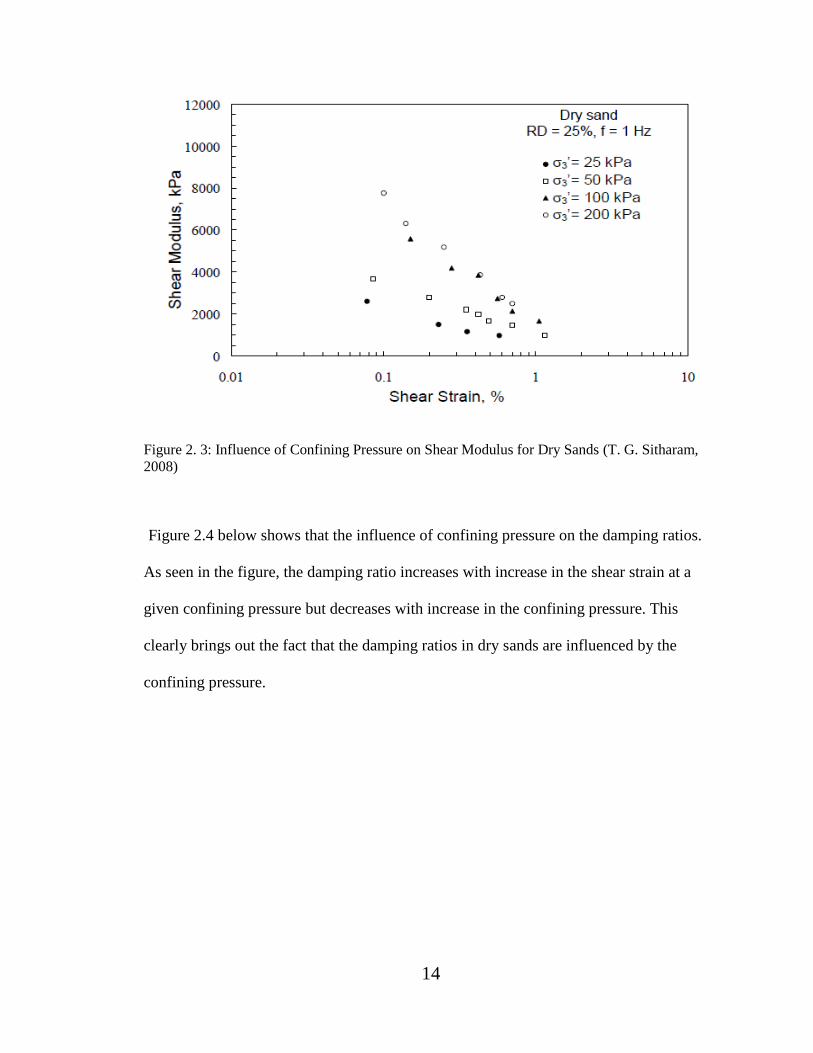
Figure 2. 3: Influence of Confining Pressure on Shear Modulus for Dry Sands (T. G.
Sitharam, 2008). ................................................................................................................ 14
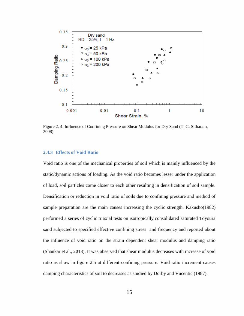
Figure 2. 4: Influence of Confining Pressure on Shear Modulus for Dry Sand (T. G.
Sitharam, 2008). ................................................................................................................ 15
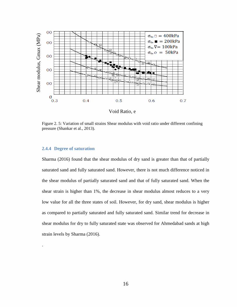
Figure 2. 5: Variation of small strains shear modulus with void ratio under different
confining pressure (Shankar et al., 2013). ........................................................................ 16
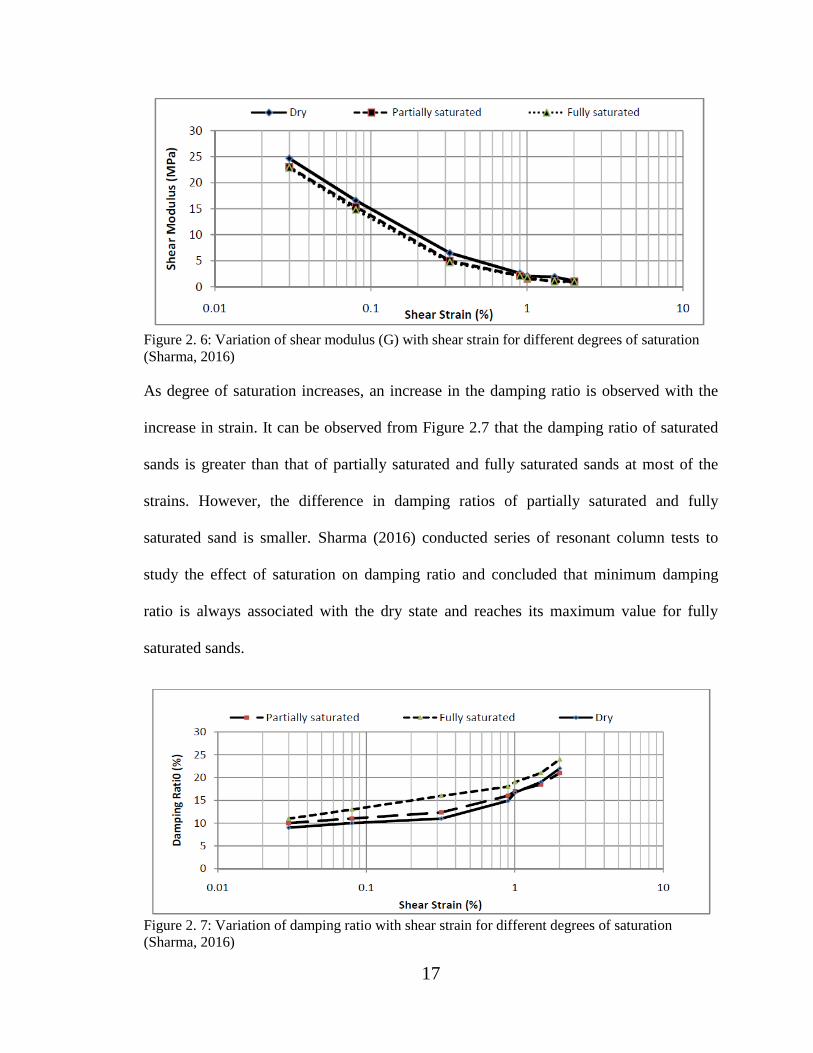
Figure 2. 6: Variation of shear modulus (G) with shear strain for different degrees of
saturation (Sharma, 2016) ................................................................................................. 17
Figure 2. 7: Variation of damping ratio with shear strain for different degrees of
saturation (Sharma, 2016) ................................................................................................. 17
Figure 2. 8: Variation of normalized shear modulus (G/Gmax) with shear strain for
different degrees of saturation (Sharma, 2016) ............................................................... 18
Figure 2. 9: Shear modulus and number of cycles at 25% RD (T. G. Sitharam, 2008)... 19
Figure 2. 10: Relationship between Damping ratio and number of cycles at 25% RD for
sand (T. G. Sitharam, 2008). ............................................................................................. 20
Figure 2. 11: Variation of Normalized shear modulus and shear strain (Muge, 2016) .... 21
Figure 2. 12: Variation of damping ratio and shear strain (Muge, 2016) ......................... 22
Figure 2. 13: Relations between G/Gmax versus γc and λ versus γc, Curves and Soil
Plasticity (PI) for normally and overconsolidated soils (Vucetic & Dobry, 1991) .......... 23
Figure 3. 1: Map of Jimma town with its administrative Kebeles .................................... 25
Figure 4. 1: Sample assembled on the cyclic simple shear equipment ............................. 28
Figure 4- 2: Brass ring ...................................................................................................... 31
Figure 4. 3: Compression stage of soil specimen of TP1 at 5% using 100 kPa ............... 32
Figure 4. 4: Sinusoidal wave shapes for 2.5% strain and 1Hz and for three cycles ......... 34
Figure 4. 5: Shear strain versus Number of cycle/Time ................................................... 37
x
Figure 4. 6: Shear stress versus Number of cycle/Time ................................................... 37
Figure 4. 7: Shear stress vs. shear strain (hysteresis loops) @ 200 kPa ........................... 38
Figure 4. 8: The hysteresis loop and triangle plotted using table 4.4 stress and strain ..... 40
Figure 5. 1: Effect of cyclic shear strain on the values of damping ratio ......................... 44
Figure 5. 2: Effect of cyclic shear strain on the values of shear modulus (MPa) ............. 45
Figure 5. 3: Effect of vertical stress on shear modulus (MPa) .......................................... 45
Figure 5. 4: Effect of vertical stress on damping ratio (%) ............................................... 46
Figure 5. 5: Effects of number of loading cycles on the value of damping ratio (%) ....... 46
Figure 5. 6: Effects of number of loading cycles on the value of shear modulus (MPa) . 47
Figure 5. 7: Effects of void ratio on the values of shear modulus (MPa) ......................... 47
Figure 5. 8: Effects of plasticity index on the values of damping ratio (%) ..................... 48
Figure 5. 9: Effects of plasticity index on the values of shear modulus (MPa) ................ 48
Figure 5. 10: Effect of plasticity index on normalized shear modulus (G/Gmax) ............ 51
Figure 5. 11: (G/Gmax) of clayey silt soil with curve drawn by Abenezer (2017) .......... 52
Figure 5. 12 (G/Gmax) of silty clay soil with curve drawn by Mengesha (2013) ............ 53
Figure 5. 13: (G/Gmax) of silty clay soil with curve drawn by Tesfaye (2012) ............... 53
Figure 5. 14: (G/Gmax) of clayey silt soil with curve drawn by Abraham (2014).......... 53
Figure 5. 15: (G/Gmax) of silty clay soil with curve drawn by Ayalew (2013) ............... 54
Figure 5. 16: Damping ratio of silty clay soil with curve drawn by Ayalew (2013) ........ 55
Figure 5. 17: Damping ratio of silty clay soil with curve drawn by Mengesha (2013) .... 55
Figure 5. 18: Damping ratio of silty clay soil with curves drawn by Abraham (2014) .... 55
Figure A- 1: Water content versus No. blow .................................................................... 63
Figure A- 2: Particle size distribution curve for TP1 ........................................................ 64
Figure A- 3: Water content versus No. blow .................................................................... 63
Figure A- 4: Particle size distribution curve for TP2 ........................................................ 64
Figure A- 5: Water content versus No. blow .................................................................... 63
Figure A- 6: Particle size distribution curve for TP3 ........................................................ 64
Figure A- 7: Water content versus No. blow .................................................................... 65
Figure A- 8: Particle size distribution curve for TP4 ........................................................ 65
Figure A- 9: Sample preparation and positioning it on the testing equipment ................. 66
Figure B- 1: Consolidation pressure versus void ratio for TP1 ........................................ 68
xi
Figure B- 2: Consolidation pressure versus void ratio for TP2 ........................................ 70
Figure C- 1: Shear strain vs number of loading cycles (γ =2.5%, σ'v =100 kPa) of TP1 . 71
Figure C- 2: Shear stress vs number of loading cycles (γ =2.5%, σ'v =100 kPa) of TP1 . 72
Figure C- 3: Shear stress vs shear strain (γ =2.5%, σ'v =100 kPa) of TP1 ........................ 72
Figure C- 4: Shear strain vs number of loading cycles (γ = 5%, σ'v =400 kPa) of TP2 ... 72
Figure C- 5: Shear stress vs number of loading cycles (γ =5%, σ'v =400 kPa) of TP2 .... 73
Figure C- 6: Shear stress vs shear strain (γ =5%, σ'v =400 kPa) of TP2 ........................... 73
Figure C- 7: Shear strain vs number of loading cycles (γ= 2.5%, σ'v =400 kPa) of TP2 . 74
Figure C- 8: Shear stress vs. number of loading cycles (γ=2.5%, σ'v =400 kPa) of TP2 . 74
Figure C- 9: Shear stress vs shear strain (γ =2.5%, σ'v =400 kPa) of TP2 ........................ 75
Figure C- 10: Shear strain vs number of loading cycles (γ= 2.5%, σ'v =250 kPa) of TP2 75
Figure C- 11: Shear stress vs number of loading cycles (γ =2.5%, σ'v =250 kPa) of TP2 76
Figure C- 12: Shear stress vs shear strain (γ =2.5%, σ'v =250 kPa) of TP2 ...................... 76
Figure C- 13: Shear strain vs number of loading cycles (γ = 5%, σ'v =250 kPa) of TP2 . 77
Figure C- 14: Shear stress vs number of loading cycles (γ =5%, σ'v =250 kPa) of TP2 .. 77
Figure C- 15: Shear stress vs shear strain (γ =5%, σ'v =250 kPa) of TP2 ........................ 78
Figure C- 16: Shear strain vs number of loading cycles (γ= 2.5%, σ'v =100 kPa),TP2 .... 78
Figure C- 17: Shear stress vs number of loading cycles (γ =2.5%, σ'v =100 kPa) of TP2 79
Figure C- 18: Shear stress vs shear strain (γ =2.5%, σ'v =100 kPa) of TP2 ...................... 79
Figure C- 19: Shear strain vs number of loading cycles (γ = 5%, σ'v =100 kPa) of TP2 . 80
Figure C- 20: Shear stress vs number of loading cycles (γ= 5%, σ'v =100 kPa) of TP2 .. 80
Figure C- 21: Shear stress vs shear strain (γ = 5%, σ'v =100 kPa) of TP2 ........................ 81
Figure C- 22: Shear strain vs number of loading cycles (γ = 5%, σ'v =250 kPa) of TP1 . 81
Figure C- 23: Shear stress vs number of loading cycles (γ= 5%, σ'v =250 kPa) of TP1 .. 82
Figure C- 24: Shear stress vs shear strain (γ = 5%, σ'v =250 kPa) of TP1 ........................ 82
Figure D- 1: Effect of vertical stress on shear modulus under for TP2 ............................ 87
Figure D- 2: Effect of vertical stress on damping ratio forTP2 ........................................ 87
Figure D- 3: Effects of number of cyclic loading cycles on the value of shear modulus . 88
Figure D- 4: Effects of number of cyclic loading cycles on the value of damping ratio .. 88
Figure D- 5: Effect of axial stress on normalized shear modulus (G/Gmax) ................... 89
Figure D- 6: Effect of axial stress on normalized shear modulus (G/Gmax) ................... 89
xii
ABBREVIATIONS
a Parameter related to plastic index
ASTM American Society for Testing Materials
standard
Aloop Loop area
D Damping ratio
e Void ratio
Eq Equation
G Dynamic shear modulus
Gmax Maximum Dynamic shear modulus
Gs Specific gravity of soil
Ko Coefficient of lateral earth pressure at rest
LL Liquid limit
Lvdt Linear variable differential transducer
Pc Pre-consolidation pressure
PI Plastic index
PL Plastic Limit
OCR Over consolidation ratio
MH silty clay
TP Test pit
WD energy dissipated in one cycle of loading
WS Maximum strain energy stored during the cycle
vs Shear wave velocity
γ Shear strain
ρ Density of soil
σ Normal stress
σ'o Effective confining stress
σ'v Effective vertical stress
τ Shear stress
1
CHAPTER ONE
INTRODUCTION
1.1 Background
Geotechnical investigation which determines the dynamic loading effect is very essential.
Among the dynamic loading earthquake is one of the natural hazards that destroys
billions of dollars properties and kills countless lives annually.
The town of Jimma is found in southwest part of Ethiopia at 354 km distance from the
capital Addis Ababa. Currently there is a dramatic increase of population growth and
industrialization with infrastructures like high rise building, residence houses, bridges,
airport, Industry Park and dams near and in the city .Additionally, the railway project
which will connect south Sudan to the capital will be part of the city. On December 19,
2010 earth quake occurred near Hosanna town 70miles East of Jimma town with a
magnitude of 5.2 mb. It caused significant damage on several buildings in Hosanna and
the shaking was felt from Mizan town in the south as far as Addis Ababa in the north. It
was also strongly felt in Jimma town and over 26 Jimma University students were injured
those accommodated in dormitory buildings. There also damages to reinforced concrete
frame and slab of dormitory buildings was observed. Even if the city has the above
infrastructures and record of seismic hazard, the dynamic properties of soil in the vicinity
have not been investigated so far.
In this study presents result of representative samples from the excavated pits collected
and tested for the determination of field test, index properties test and cyclic simple shear
test. The behavior of soils is described and the implications of the test results with
2
published data are discussed. The dynamic soil properties can be used as input parameters
for the design of foundations for machinery and vibrating equipment, analysis of slope
stability of embankments under earthquake loading conditions and also used to model
soil behavior under dynamic loading.
1.2 Objective of the study
1.2.1 General objective
The major objective of this research is to determine the dynamic shear modulus and
Damping ratio values of typical soils found in Jimma town.
1.2.2 Specific objective
To determine the index properties and classify the soil.
To determine bulk density of the soil using core cutter method.
To determine shear modulus and damping ratio using cyclic simple shear tests.
1.3 Methodology
To meet the above objectives, typical soil samples were collected from four pits
excavated up to 3.0 m depth each for the investigation which are representative to
characterize the dominant soils in the study area. Cyclic simple shear tests were then
performed, to determine the stiffness and damping characteristics of the soil samples.
In addition to meet this goal the following laboratory tests were conducted:
In-situ density and moisture content
Particle size analysis
Specific gravity
Consolidation tests
3
1.4 Scope and limitation of the study
The dynamic properties of soil are influenced by soil type and specific location of where
the soil sample is collected. The collected samples may not fully represent all the soil
profile in Jimma town as it is limited to four pits and the samples were taken from the
depth of only three meters despite the fact that seismic related ground response behavior
significantly affected by 30 m loose layer. In addition to sampling limitation the tests
were conducted using cyclic simple shear testing equipment due to unavailability of more
sophisticated facilities.
1.5 Organization of the thesis
The study consists of six Chapters and appendixes. The background information is presented
under Chapter one which mainly focus on introduction, objective, and scope and limitation of
the thesis. Literature review is mainly presented in second Chapter which includes index
property and dynamic properties of soils. Chapter three discusses about study area, geology
and formation of soil found in Jimma. The sample collection, sample preparation, overview
of cyclic simple shear apparatus, experimental programme and calculations are discussed in
chapter four. In fifth chapter discussion of test results and some comparison with previous
study is presented. The sixth Chapter is conclusion and recommendation of the thesis.

4
CHAPTER TWO
LITERATURE REVIEW
2.1 Introduction
The geological conditions, topographic characteristics and climatic conditions play a vital
role in the formation of soil in any region. Soil is generally considered as a three-phase
system (air, water and solid) causing significant changes in the system characteristics due
to interaction of these phases under applied static and/or dynamic load. Static loads
remain unchanged over space and time, while dynamic load represents loading conditions
which vary both in their direction/position and/or magnitude (Shankar et al., 2013).
Several researchers have been involved in exploring the complex behavior of soils under
various types of loading conditions.
As Thirugnanasampanther (2012) have demonstrated soils are subjected to cyclic loading
during earthquakes and consequently it might lose their shear strength partially or
completely .As a result, natural and man-made structures founded on soils will be
exposed to stability problems such as unpredicted deformations, settlement or
catastrophic collapse due to dynamic loading of earthquakes, operation of machinery,
bomb blasting, wind or wave action of water, construction operation, fast moving
transportation media and others. Therefore, an assessment of the loading conditions and a
better understanding of the dynamic properties of soils will help in the design of seismic
resistant earth structures such as foundations, dams, bridges, and retaining structures.
Further, evaluation of liquefaction is very vital in sites located within earthquake prone
regions or heavily populated areas.
5
Dynamic properties of soils are used to evaluate the dynamic response of soils at different
strain levels in geotechnical engineering. Shear modulus and material damping ratio are
the most important dynamic properties of soils (Moayerian, 2012) and determination of
these properties is an utmost critical and important aspect of geotechnical engineering
problems.
2.2 Dynamic soil properties
The response of soil which is subjected to dynamic loads is governed by dynamic soil
properties. To determine these properties the response obtained after different loading
case need to be analyzed. A typical soil subjected to cyclic loading exhibits hysteresis
response. The hysteresis loop produced from the cyclic loading of a typical soil can be
described by the path of the loop itself or by two parameters that describe its general
shape. These parameters are the inclination and the breath of the hysteresis loop, shear
modulus and damping ratio (Luna and Jadi, 2000). As the strain amplitude of cyclic
loading is varied, different size of loops will be developed (Shankar et al., 2013).
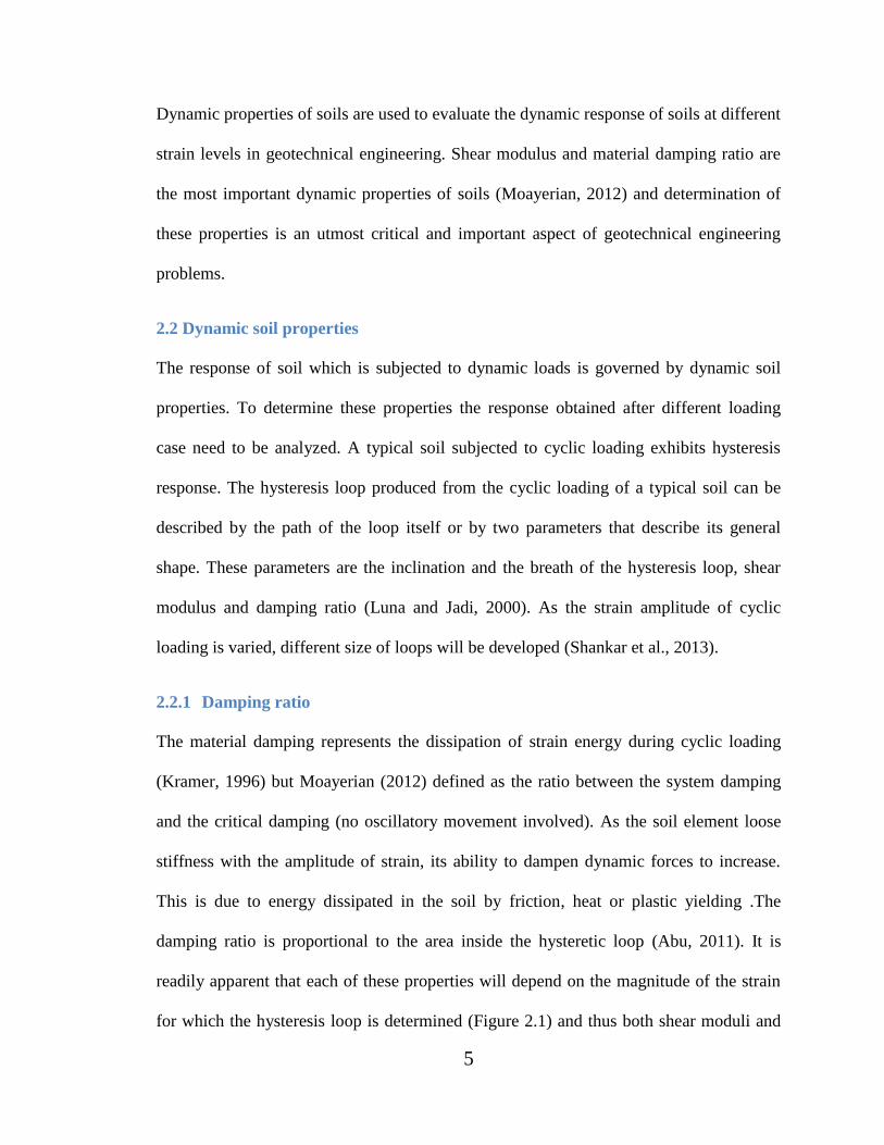
2.2.1 Damping ratio
The material damping represents the dissipation of strain energy during cyclic loading
(Kramer, 1996) but Moayerian (2012) defined as the ratio between the system damping
and the critical damping (no oscillatory movement involved). As the soil element loose
stiffness with the amplitude of strain, its ability to dampen dynamic forces to increase.
This is due to energy dissipated in the soil by friction, heat or plastic yielding .The
damping ratio is proportional to the area inside the hysteretic loop (Abu, 2011). It is
readily apparent that each of these properties will depend on the magnitude of the strain
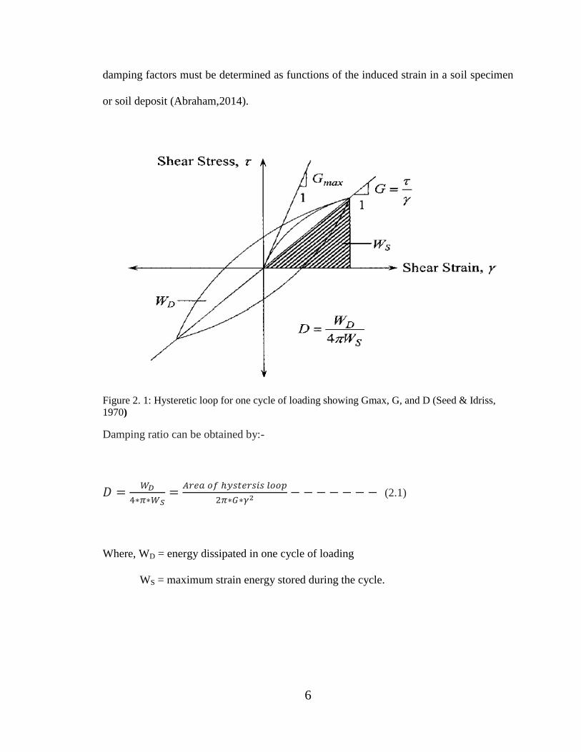
for which the hysteresis loop is determined (Figure 2.1) and thus both shear moduli and
6
damping factors must be determined as functions of the induced strain in a soil specimen
or soil deposit (Abraham,2014).
Figure 2. 1: Hysteretic loop for one cycle of loading showing Gmax, G, and D (Seed & Idriss,
1970)
Damping ratio can be obtained by:-
(2.1)
Where, WD = energy dissipated in one cycle of loading
WS = maximum strain energy stored during the cycle.
7
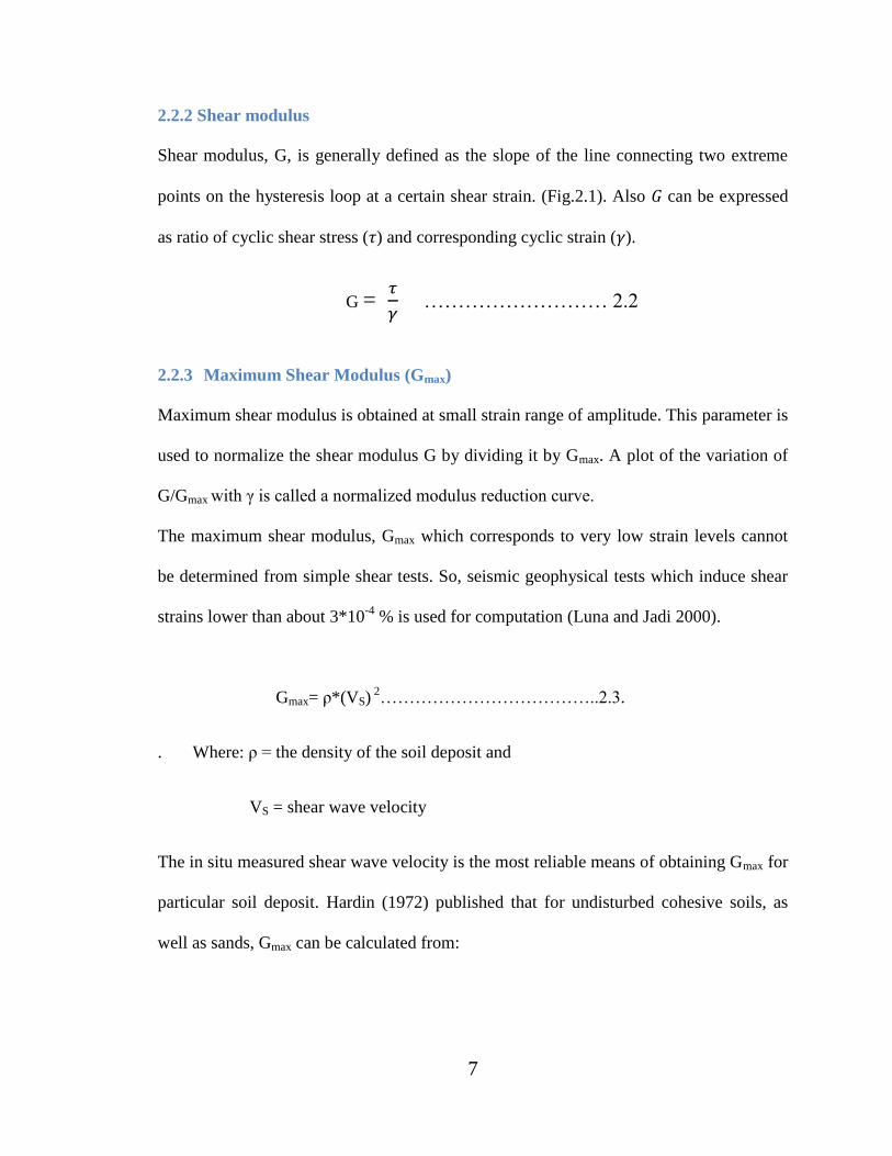
2.2.2 Shear modulus
Shear modulus, G, is generally defined as the slope of the line connecting two extreme
points on the hysteresis loop at a certain shear strain. (Fig.2.1). Also 𝐺 can be expressed
as ratio of cyclic shear stress (𝜏) and corresponding cyclic strain (𝛾).
G =
……………………… 2.2
2.2.3 Maximum Shear Modulus (Gmax)
Maximum shear modulus is obtained at small strain range of amplitude. This parameter is
used to normalize the shear modulus G by dividing it by Gmax. A plot of the variation of
G/Gmax with γ is called a normalized modulus reduction curve.
The maximum shear modulus, Gmax which corresponds to very low strain levels cannot
be determined from simple shear tests. So, seismic geophysical tests which induce shear
strains lower than about 3*10-4
% is used for computation (Luna and Jadi 2000).
Gmax= ρ*(VS) 2
………………………………..2.3.
. Where: ρ = the density of the soil deposit and
VS = shear wave velocity
The in situ measured shear wave velocity is the most reliable means of obtaining Gmax for
particular soil deposit. Hardin (1972) published that for undisturbed cohesive soils, as
well as sands, Gmax can be calculated from:
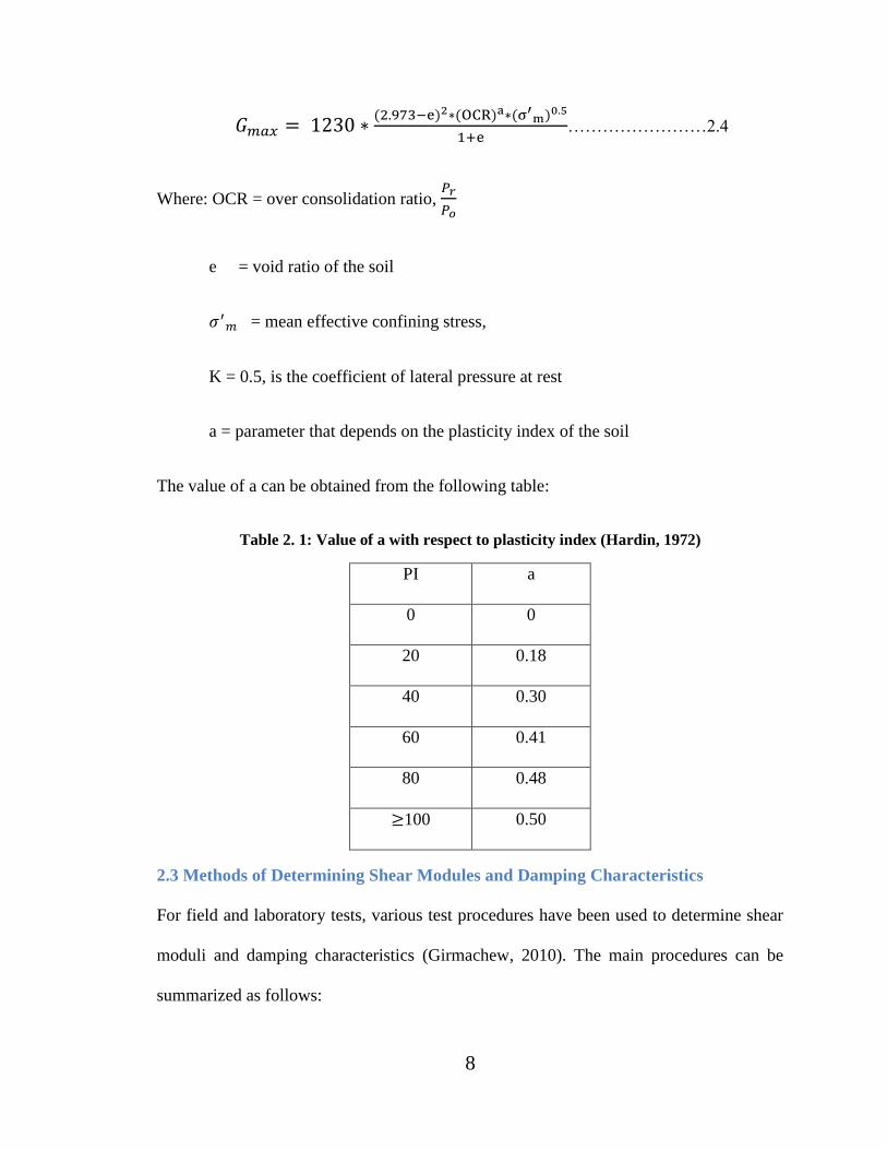
8
𝐺
……………………2.4
Where: OCR = over consolidation ratio,
e = void ratio of the soil
= mean effective confining stress,
K = 0.5, is the coefficient of lateral pressure at rest
a = parameter that depends on the plasticity index of the soil
The value of a can be obtained from the following table:
Table 2. 1: Value of a with respect to plasticity index (Hardin, 1972)
PI a
0 0
20 0.18
40 0.30
60 0.41
80 0.48
100 0.50
2.3 Methods of Determining Shear Modules and Damping Characteristics
For field and laboratory tests, various test procedures have been used to determine shear
moduli and damping characteristics (Girmachew, 2010). The main procedures can be
summarized as follows:
9
2.3.1 Direct determination of stress-strain relationships
Hysteretic stress-strain relationships of the type shown in Figure 2.1 may be determined
in the laboratory by means of triaxial compression tests, simple shear tests or torsional
shear tests conducted under cyclic loading conditions. Seed and Edriss (1970) studied
these procedures are useful for measuring shear modules and damping factors under
moderate to relatively high strains (0.01<γ<5%). In this paper the test was performed
using simple shear test among the given method above.
2.3.2 Forced vibration tests
Forced vibration tests, involving the determination of resonant frequencies and
measurement of response with different frequencies have been used to determine both
shear modules and damping factors. Test conditions in the laboratory have included the
application of longitudinal vibrations and tensional vibrations to cylindrical samples or
shear vibrations to layers of soil placed on a shaking table. As studied by Seed and Edriss
(1970) these procedures are useful for determining properties at relatively low to
moderate strain levels (10-4
< γ <10-2
%).
2.3.3 Free vibration tests
Free vibration tests, in which measurements are made of the decay in response of a soil
sample or soil deposit, have been used to measure both shear modules and damping
factors for soils. Seed and Edriss (1970) published that methods of excitation are
essentially similar to those used for forced vibration tests, but the procedures can be used
for measurement of soil characteristics at relatively low to moderately high strain levels
(10-3
< γ <1%).
10
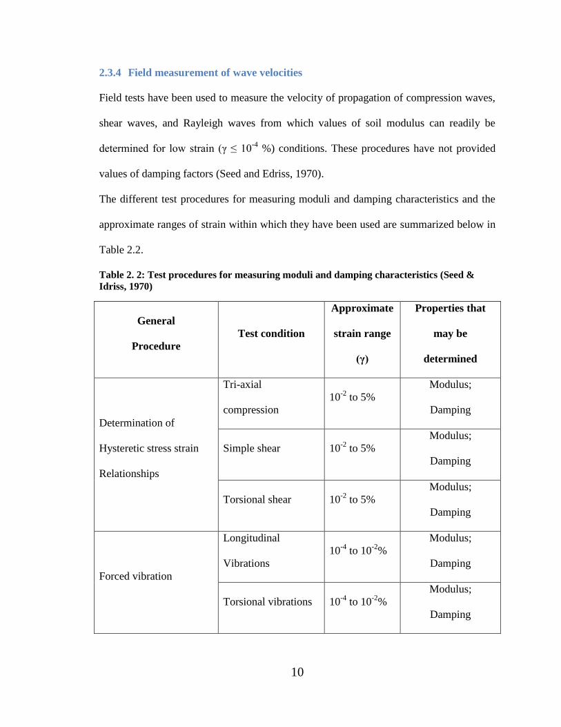
2.3.4 Field measurement of wave velocities
Field tests have been used to measure the velocity of propagation of compression waves,
shear waves, and Rayleigh waves from which values of soil modulus can readily be
determined for low strain (γ ≤ 10-4
%) conditions. These procedures have not provided
values of damping factors (Seed and Edriss, 1970).
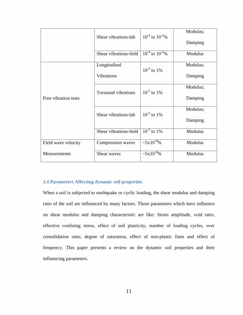
The different test procedures for measuring moduli and damping characteristics and the
approximate ranges of strain within which they have been used are summarized below in
Table 2.2.
Table 2. 2: Test procedures for measuring moduli and damping characteristics (Seed &
Idriss, 1970)
General
Procedure
Test condition
Approximate
strain range
(γ)
Properties that
may be
determined
Determination of
Hysteretic stress strain
Relationships
Tri-axial
compression
10-2
to 5%
Modulus;
Damping
Simple shear 10-2
to 5%
Modulus;
Damping
Torsional shear 10-2
to 5%
Modulus;
Damping
Forced vibration
Longitudinal
Vibrations
10-4
to 10-2
%
Modulus;
Damping
Torsional vibrations 10-4
to 10-2
%
Modulus;
Damping
11
Shear vibrations-lab 10-4
to 10-2
%
Modulus;
Damping
Shear vibrations-field 10-4
to 10-2
% Modulus
Free vibration tests
Longitudinal
Vibrations
10-3
to 1%
Modulus;
Damping
Torsional vibrations 10-3
to 1%
Modulus;
Damping
Shear vibrations-lab 10-3
to 1%
Modulus;
Damping
Shear vibrations-field 10-3
to 1% Modulus
Field wave velocity
Measurements
Compression waves ~5x10⁻⁴
% Modulus
Shear waves ~5x10⁻⁴
% Modulus
2.4 Parameters Affecting dynamic soil properties
When a soil is subjected to earthquake or cyclic loading, the shear modulus and damping
ratio of the soil are influenced by many factors. Those parameters which have influence
on shear modulus and damping characteristic are like: Strain amplitude, void ratio,
effective confining stress, effect of soil plasticity, number of loading cycles, over
consolidation ratio, degree of saturation, effect of non-plastic fines and effect of
frequency. This paper presents a review on the dynamic soil properties and their
influencing parameters.
12
2.4.1 Effect of non-plastic fine Materials
The role of non-plastic fines in large-strain phenomenon such as Liquefaction has been
studied extensively. Yamamuro and Lade (1998) discussed that, the induction of
liquefaction can be described in terms of particle contacts shearing against each other in
the small to intermediate strain range even if liquefaction itself results in large strains in
the soil.
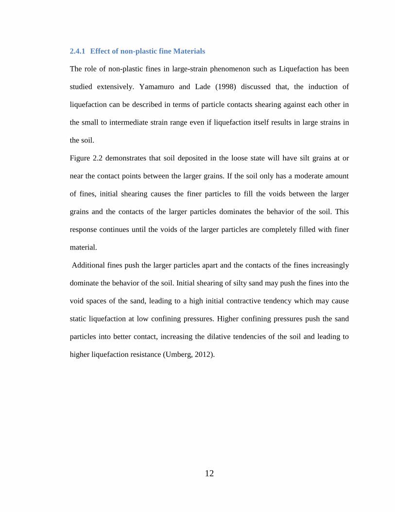
Figure 2.2 demonstrates that soil deposited in the loose state will have silt grains at or
near the contact points between the larger grains. If the soil only has a moderate amount
of fines, initial shearing causes the finer particles to fill the voids between the larger
grains and the contacts of the larger particles dominates the behavior of the soil. This
response continues until the voids of the larger particles are completely filled with finer
material.
Additional fines push the larger particles apart and the contacts of the fines increasingly
dominate the behavior of the soil. Initial shearing of silty sand may push the fines into the
void spaces of the sand, leading to a high initial contractive tendency which may cause
static liquefaction at low confining pressures. Higher confining pressures push the sand
particles into better contact, increasing the dilative tendencies of the soil and leading to
higher liquefaction resistance (Umberg, 2012).
13
Figure 2. 2: Hypothetical Particle Structure of Loose Silty Sand with Low Silt Content (a) As
Deposited and (b) After Densification due to Shearing. (Yamamuro & Lade, 1999)
2.4.2 Effect of Confining Pressure
Shear modulus and damping ratio are significantly affected by confining pressure
(Shankar et al., 2013). The influence of confining pressure on the shear modulus is shown
in Figure 2.3. It may be noticed from the figure that there is considerable influence of
confining pressure on shear modulus. As the confining pressure increases the shear
modulus increases significantly, however the shear modulus follows a converging trend
towards larger shear strains irrespective of the confining pressure to which the samples
are subjected (T. G. Sitharam, 2008).
Sand grains
(a) Particle structure as
deposited in loose state
Silt grains near
contact points
Large grains move
together creating large
initial volume reduction
Large grains come into
better contact increasing
dilatants tendencies
(b) Particle structure
compressed and sheared
14
Figure 2. 3: Influence of Confining Pressure on Shear Modulus for Dry Sands (T. G. Sitharam,
2008)
Figure 2.4 below shows that the influence of confining pressure on the damping ratios.
As seen in the figure, the damping ratio increases with increase in the shear strain at a
given confining pressure but decreases with increase in the confining pressure. This
clearly brings out the fact that the damping ratios in dry sands are influenced by the
confining pressure.
15
Figure 2. 4: Influence of Confining Pressure on Shear Modulus for Dry Sand (T. G. Sitharam,
2008)
2.4.3 Effects of Void Ratio
Void ratio is one of the mechanical properties of soil which is mainly influenced by the
static/dynamic actions of loading. As the void ratio becomes lesser under the application
of load, soil particles come closer to each other resulting in densification of soil sample.
Densification or reduction in void ratio of soils due to confining pressure and method of
sample preparation are the main causes increasing the cyclic strength. Kakusho(1982)
performed a series of cyclic triaxial tests on isotropically consolidated saturated Toyoura
sand subjected to specified effective confining stress and frequency and reported about
the influence of void ratio on the strain dependent shear modulus and damping ratio
(Shankar et al., 2013). It was observed that shear modulus decreases with increase of void
ratio as show in figure 2.5 at different confining pressure. Void ratio increment causes
damping characteristics of soil to decreases as studied by Dorby and Vucentic (1987).
16
Figure 2. 5: Variation of small strains Shear modulus with void ratio under different confining
pressure (Shankar et al., 2013).
2.4.4 Degree of saturation
Sharma (2016) found that the shear modulus of dry sand is greater than that of partially
saturated sand and fully saturated sand. However, there is not much difference noticed in
the shear modulus of partially saturated sand and that of fully saturated sand. When the
shear strain is higher than 1%, the decrease in shear modulus almost reduces to a very
low value for all the three states of soil. However, for dry sand, shear modulus is higher
as compared to partially saturated and fully saturated sand. Similar trend for decrease in
shear modulus for dry to fully saturated state was observed for Ahmedabad sands at high
strain levels by Sharma (2016).
.
Void Ratio, e
Shea
r m
od
ulu
s, G
max
(M
Pa)
17
Figure 2. 6: Variation of shear modulus (G) with shear strain for different degrees of saturation
(Sharma, 2016)
As degree of saturation increases, an increase in the damping ratio is observed with the
increase in strain. It can be observed from Figure 2.7 that the damping ratio of saturated
sands is greater than that of partially saturated and fully saturated sands at most of the
strains. However, the difference in damping ratios of partially saturated and fully
saturated sand is smaller. Sharma (2016) conducted series of resonant column tests to
study the effect of saturation on damping ratio and concluded that minimum damping
ratio is always associated with the dry state and reaches its maximum value for fully
saturated sands.
Figure 2. 7: Variation of damping ratio with shear strain for different degrees of saturation
(Sharma, 2016)
18
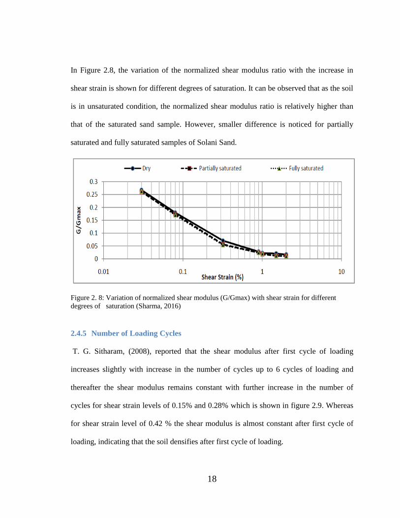
In Figure 2.8, the variation of the normalized shear modulus ratio with the increase in
shear strain is shown for different degrees of saturation. It can be observed that as the soil
is in unsaturated condition, the normalized shear modulus ratio is relatively higher than
that of the saturated sand sample. However, smaller difference is noticed for partially
saturated and fully saturated samples of Solani Sand.
Figure 2. 8: Variation of normalized shear modulus (G/Gmax) with shear strain for different
degrees of saturation (Sharma, 2016)
2.4.5 Number of Loading Cycles
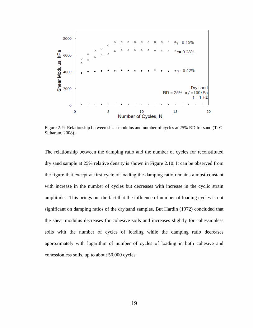
T. G. Sitharam, (2008), reported that the shear modulus after first cycle of loading
increases slightly with increase in the number of cycles up to 6 cycles of loading and
thereafter the shear modulus remains constant with further increase in the number of
cycles for shear strain levels of 0.15% and 0.28% which is shown in figure 2.9. Whereas
for shear strain level of 0.42 % the shear modulus is almost constant after first cycle of
loading, indicating that the soil densifies after first cycle of loading.
19
Figure 2. 9: Relationship between shear modulus and number of cycles at 25% RD for sand (T. G.
Sitharam, 2008).
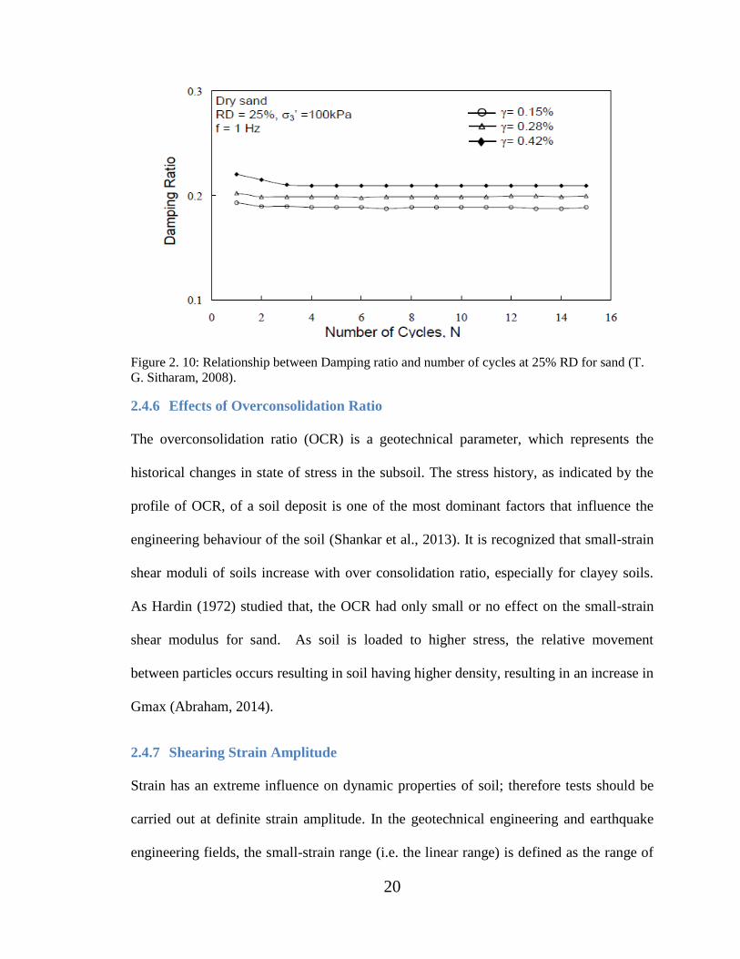
The relationship between the damping ratio and the number of cycles for reconstituted
dry sand sample at 25% relative density is shown in Figure 2.10. It can be observed from
the figure that except at first cycle of loading the damping ratio remains almost constant
with increase in the number of cycles but decreases with increase in the cyclic strain
amplitudes. This brings out the fact that the influence of number of loading cycles is not
significant on damping ratios of the dry sand samples. But Hardin (1972) concluded that
the shear modulus decreases for cohesive soils and increases slightly for cohessionless
soils with the number of cycles of loading while the damping ratio decreases
approximately with logarithm of number of cycles of loading in both cohesive and
cohessionless soils, up to about 50,000 cycles.
20
Figure 2. 10: Relationship between Damping ratio and number of cycles at 25% RD for sand (T.
G. Sitharam, 2008).
2.4.6 Effects of Overconsolidation Ratio
The overconsolidation ratio (OCR) is a geotechnical parameter, which represents the
historical changes in state of stress in the subsoil. The stress history, as indicated by the
profile of OCR, of a soil deposit is one of the most dominant factors that influence the
engineering behaviour of the soil (Shankar et al., 2013). It is recognized that small-strain
shear moduli of soils increase with over consolidation ratio, especially for clayey soils.
As Hardin (1972) studied that, the OCR had only small or no effect on the small-strain
shear modulus for sand. As soil is loaded to higher stress, the relative movement
between particles occurs resulting in soil having higher density, resulting in an increase in
Gmax (Abraham, 2014).
2.4.7 Shearing Strain Amplitude
Strain has an extreme influence on dynamic properties of soil; therefore tests should be
carried out at definite strain amplitude. In the geotechnical engineering and earthquake
engineering fields, the small-strain range (i.e. the linear range) is defined as the range of
21
shear strain amplitudes over which the dynamic properties of soils (shear modulus, G,
and material damping ratio, D) are constant. Because in that strain range the shear
modulus is constant with the maximum value and the material damping ratio is constant
with the minimum value. These dynamic properties are called Gmax and Dmin,
respectively. In the technical literature, the small-strain range of sands is often described
by strains less than 10-3
% (Shin, 2014). As strain increases beyond the small-strain
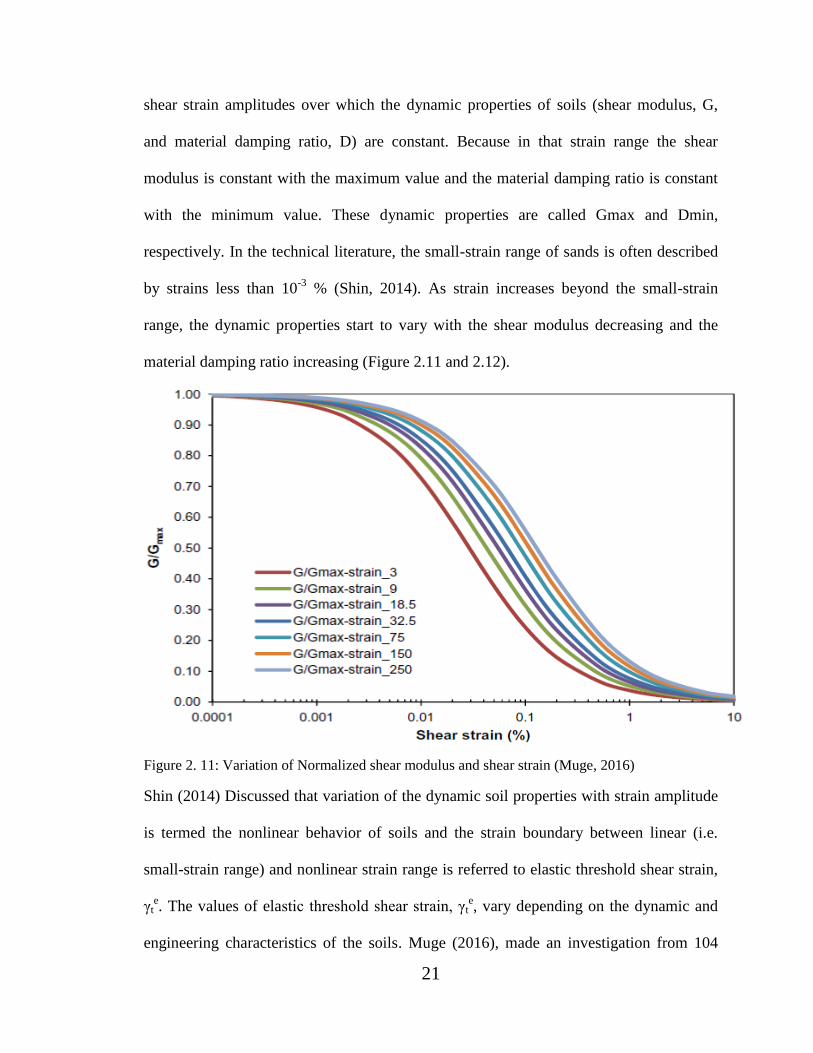
range, the dynamic properties start to vary with the shear modulus decreasing and the
material damping ratio increasing (Figure 2.11 and 2.12).
Figure 2. 11: Variation of Normalized shear modulus and shear strain (Muge, 2016)
Shin (2014) Discussed that variation of the dynamic soil properties with strain amplitude
is termed the nonlinear behavior of soils and the strain boundary between linear (i.e.
small-strain range) and nonlinear strain range is referred to elastic threshold shear strain,
γte. The values of elastic threshold shear strain, γt
e, vary depending on the dynamic and
engineering characteristics of the soils. Muge (2016), made an investigation from 104
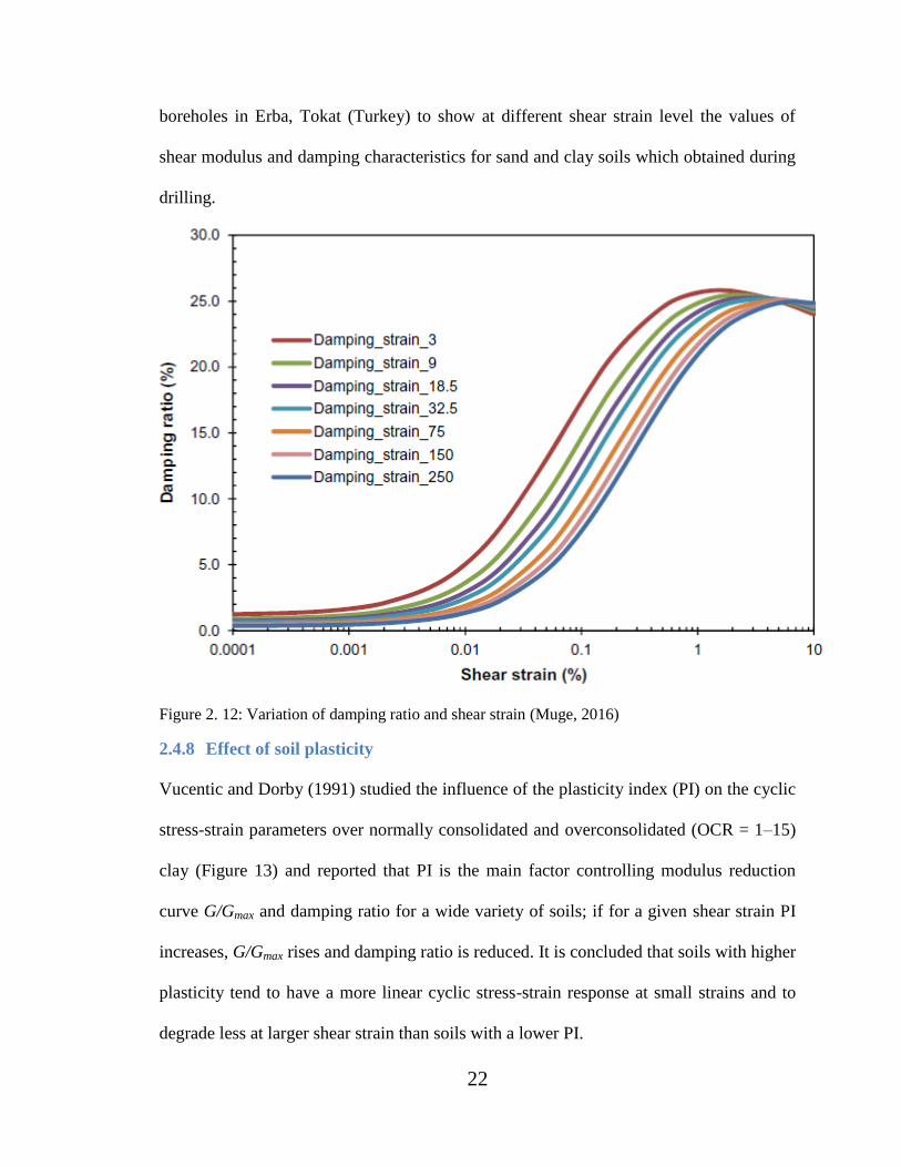
22
boreholes in Erba, Tokat (Turkey) to show at different shear strain level the values of
shear modulus and damping characteristics for sand and clay soils which obtained during
drilling.
Figure 2. 12: Variation of damping ratio and shear strain (Muge, 2016)
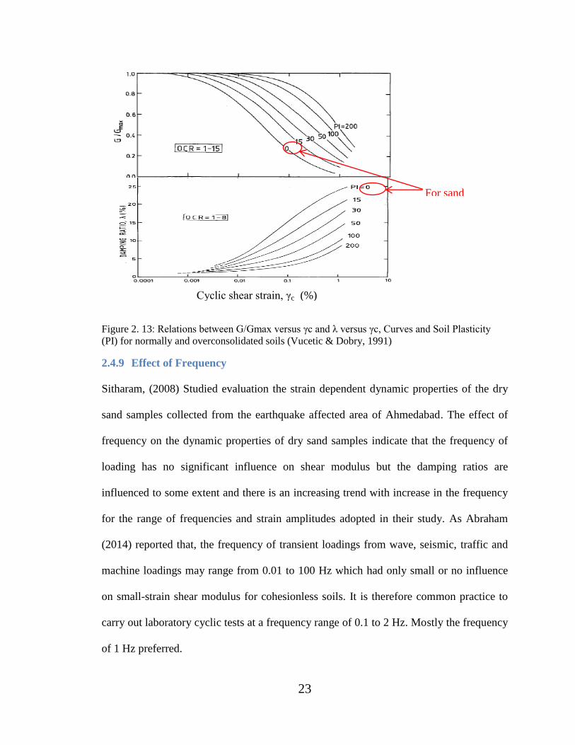
2.4.8 Effect of soil plasticity
Vucentic and Dorby (1991) studied the influence of the plasticity index (PI) on the cyclic
stress-strain parameters over normally consolidated and overconsolidated (OCR = 1–15)
clay (Figure 13) and reported that PI is the main factor controlling modulus reduction
curve G/Gmax and damping ratio for a wide variety of soils; if for a given shear strain PI
increases, G/Gmax rises and damping ratio is reduced. It is concluded that soils with higher
plasticity tend to have a more linear cyclic stress-strain response at small strains and to
degrade less at larger shear strain than soils with a lower PI.
23
Figure 2. 13: Relations between G/Gmax versus γc and λ versus γc, Curves and Soil Plasticity
(PI) for normally and overconsolidated soils (Vucetic & Dobry, 1991)
2.4.9 Effect of Frequency
Sitharam, (2008) Studied evaluation the strain dependent dynamic properties of the dry
sand samples collected from the earthquake affected area of Ahmedabad. The effect of
frequency on the dynamic properties of dry sand samples indicate that the frequency of
loading has no significant influence on shear modulus but the damping ratios are
influenced to some extent and there is an increasing trend with increase in the frequency
for the range of frequencies and strain amplitudes adopted in their study. As Abraham
(2014) reported that, the frequency of transient loadings from wave, seismic, traffic and
machine loadings may range from 0.01 to 100 Hz which had only small or no influence
on small-strain shear modulus for cohesionless soils. It is therefore common practice to
carry out laboratory cyclic tests at a frequency range of 0.1 to 2 Hz. Mostly the frequency
of 1 Hz preferred.
Cyclic shear strain, γc (%)
For sand
24
CHAPTER THREE
DESCRIPTION OF STUDY AREA
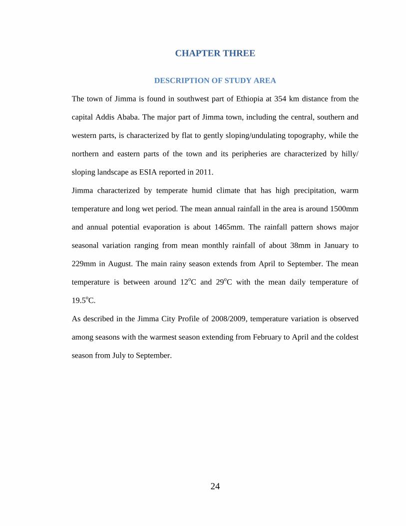
The town of Jimma is found in southwest part of Ethiopia at 354 km distance from the
capital Addis Ababa. The major part of Jimma town, including the central, southern and
western parts, is characterized by flat to gently sloping/undulating topography, while the
northern and eastern parts of the town and its peripheries are characterized by hilly/
sloping landscape as ESIA reported in 2011.
Jimma characterized by temperate humid climate that has high precipitation, warm
temperature and long wet period. The mean annual rainfall in the area is around 1500mm
and annual potential evaporation is about 1465mm. The rainfall pattern shows major
seasonal variation ranging from mean monthly rainfall of about 38mm in January to
229mm in August. The main rainy season extends from April to September. The mean
temperature is between around 12oC and 29
oC with the mean daily temperature of
19.5oC.
As described in the Jimma City Profile of 2008/2009, temperature variation is observed
among seasons with the warmest season extending from February to April and the coldest
season from July to September.
25
Figure 3. 1: Map of Jimma town with its administrative Kebeles
3.1 Geology
According to the geological map of Ethiopia 1:200,000 scale and the report compiled by
Tefera (1996) the project area is generally made up of the following major geological
formations.
Jimma Volcanics (Pjb and Pjr)
The name Jimma volcanics was given to trachybasalts and rhyolites which cover most
parts of southwestern Ethiopia.The Jimma volcanics which are considered analogous to
the Main Volcanic Sequence are a thick succession of basalts and salic rocks with basalts
dominating the lower part of most sections. It was reported K/Ar age of 42.7-30.5 Ma for
the Jimma volcanics. Two units (Jimma Basalts and Jimma Rhyolites) which show a
conformable relation can be identified. The Jimma Rhyolites being the younger of the
two units is equivalent to the Magadala Group of Kazmin of southwestern Ethiopia. The
26
Jimma volcanic almost always rests on the Precambrian basement, the unconformity
being marked by basal residual sandstone. The basalt flows form an unbroken succession
several hundred meters thick in some places. In others salic rocks are intercalated with
basalt flows close to the base or form a thick succession just above the basal basalts.
Nazret Series
The name Nazret Series was given for a thick succession of Welded fiamme ignimbrites,
pumice, ash and rhyolite flows and domes with rare intercalations of basalt flows which
occur in the MER, rift margins and adjacent plateau. In the Nazret Series attains a
thickness of up to 200 - 250 m. and tends to thin out on the escarpments. On the plateau
margins a thickness of 1 - 30 m was reported at many localities. Ignimbrites of the
Nazret Series are considered to be products of eruptions mainly from marginal centers in
the rift .In composition the ignimbrites are alkaline rhyolites with transition to peralkaline
rhyolites, pantellerites and trachytes.
Quaternary Sediments: Alluvial and lacustrine deposits consisting of sand, silt and clay.
3.1.1 Soil formation
The top most part of the pits is covered by silt, gravel and mixed crushed stone with grass
root having an average 0.34m depth below NGL. Beneath the top soil layer, there is
medium stiff to stiff, reddish and dark gray, high plastic, clayey silt/silty clay with little
sand soil are the main soil layers through the test pits.
27
CHAPTER FOUR
EXPERIMENTAL PROGRAMME
4.1. Overview of testing equipment
To determine dynamic property of any type of soils various kind of machines are
available. These include cyclic triaxial, resonant column, ultrasonic pulse, piezoelectric
bender element, cyclic simple shear and cyclic torsional shear apparatuses (Kramer,
1996). Among these machines cyclic simple shear is used for this research.
4.1.1. Cyclic simple shear testing system
The system is designed to allow a sample to be consolidated and sheared under drained
conditions. Cyclic simple shear tests can be conducted for a wider range of strain
amplitude (that is, 10-2
% to about 5%). This range is the general range of strain
encountered in the ground motion during seismic activities (Das, 1993).
The base machine consists of a simple shear load frame, an air receiver with axial
(vertical) and lateral (horizontal) loading control valves and two 5 kN actuators, built into
a specially designed floor-mounted cabinet, which also houses the Integrated Multi-Axis
Control System (IMACS) and the PC. The axial and lateral actuators are fixed to the load
frame, which supplies the reaction to the forces applied. Each actuator has an internal
displacement transducer, which relays the actuator position back to the computer. This is
very important when setting up a sample; it allows you to set enough travel for the test
duration. The top half of the area where the sample is set up is rigidly fixed and houses a
50 (70) mm diameter vertical ram in a linear bearing to allow axial movement but prevent
28
lateral movement. The bottom half is mounted on roller bearings in the same way as in a
standard shear box apparatus (UTS004, 2003).
While the specimen is being subjected to loading forces, the IMACS captures data from
the transducers and transfers these, via the USB or RS232 link, to the PC for processing,
display and storage.
The Integrated Multi-Axis Control System is a compact self- contained unit that provides
all critical control, timing and data acquisition functions for the test and the transducers.
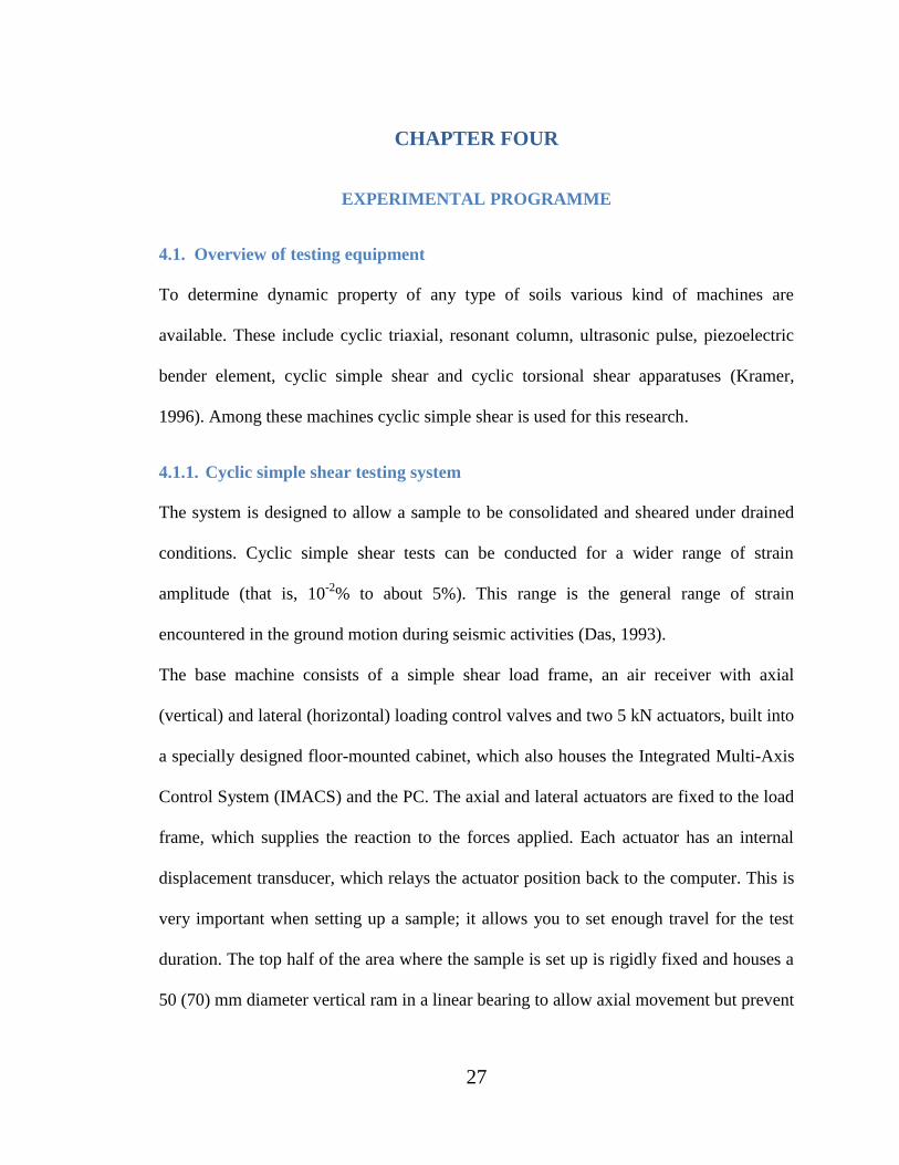
The standard sample is 70 mm diameter. The test can also be performed on 50 mm
diameter samples using the other load arm which fits with the sample size. The sample is
positioned on a pedestal with a top cap the same as a triaxial sample and covered by a
rubber membrane placed and secured with O-rings. To maintain a constant diameter (K0
conditions) the sample is laterally confined by a series of brass rings.
Figure 4. 1: Sample assembled on the cyclic simple shear equipment
4.2 Field and laboratory tests
To select sampling areas, visual site investigation which used for observation of soil
stratification from deep cuts near buildings and open areas to locate the sampling points
29
in the town. Accordingly, four representative sampling areas were selected from different
locations of the town. The selected points were Stadium (TP1), Ajip (TP2), around St.
Gebriel church (TP3) and Kitto Furdissa (TP4). Pits were excavated to a depth of three
meters below natural ground level where samples were taken starting from two and half
meters. On the selected pointes both field and laboratory tests were performed. Tests like
bulk density, index property test, one dimensional consolidation test and cyclic simple
shear tests were used to clearly identify the material tested.
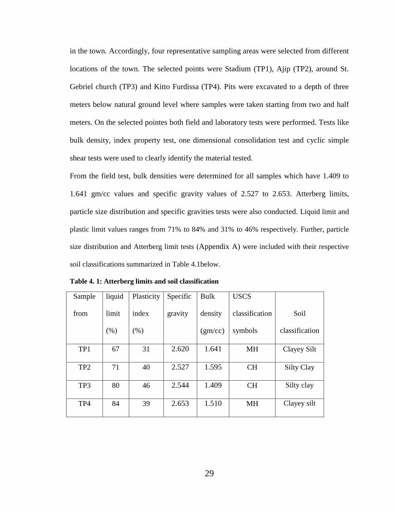
From the field test, bulk densities were determined for all samples which have 1.409 to
1.641 gm/cc values and specific gravity values of 2.527 to 2.653. Atterberg limits,
particle size distribution and specific gravities tests were also conducted. Liquid limit and
plastic limit values ranges from 71% to 84% and 31% to 46% respectively. Further, particle
size distribution and Atterberg limit tests (Appendix A) were included with their respective
soil classifications summarized in Table 4.1below.
Table 4. 1: Atterberg limits and soil classification
Sample
from
liquid
limit
(%)
Plasticity
index
(%)
Specific
gravity
Bulk
density
(gm/cc)
USCS
classification
symbols
Soil
classification
TP1 67 31 2.620 1.641 MH Clayey Silt
TP2 71 40 2.527 1.595 CH Silty Clay
TP3 80 46 2.544 1.409 CH Silty clay
TP4 84 39 2.653 1.510 MH Clayey silt
30
4.2.1 One-dimensional Consolidation
The main aim of one dimensional consolidation test is to get better understanding on
stress history of the soil under study. Additionally, the preconsolidation pressure which
used to compute the maximum shear modulus of the soil in this paper was obtained from
the test. Detailed calculation of test result is shown in Table B.1 to B.2 and graph of
Figure B-1 to B-2 in the appendix B. The preconsolidation pressure is obtained from the
graph and is found to be 65 to 85 kPa.
4.2.2 Simple cyclic shear test procedures
4.2.2.1 Preparation of specimens
The soil in the Shelby tube sample was extruded into a stainless steel ring with sharp
cutting edge having the same diameter (70 mm) as the sampling tube. The stainless steel
ring was positioned right above and in alignment with the axis of the tube during this
process. Having the ring around the specimen, allowed careful confinement and securing
of the soil specimen against disturbance after extrusion from the tube. The specimen
secured in the steel ring as per above was trimmed at the top and bottom ends to obtain a
specimen height of 20 mm. The prepared sample pushed slowly using wooden sample
extruder from string holding by hand and then specimen of 20 mm height and 70 mm
diameter sample were obtained.
4.2.2.2 Setup of cyclic simple shear testing
The machine uses highly filtered compressed air from huge compressor where it’s
required to connect everything, to fill the air chamber before beginning any type of tests.
Then, sample preparation, consolidation and cyclic shearing are common procedure in
the laboratory to carry out cyclic simple shear test. The sample is set up in the cyclic
31
simple shear equipment, which has a rigidly fixed top half and a moving bottom half. The
top half houses the vertical ram. This is housed in a linear bearing to allow vertical
movement and prevent horizontal movement. The bottom half is mounted on roller
bearings as in a standard shear box (Abraham, 2014). The sample is supported by a
rubber membrane placed and secured with O-rings.
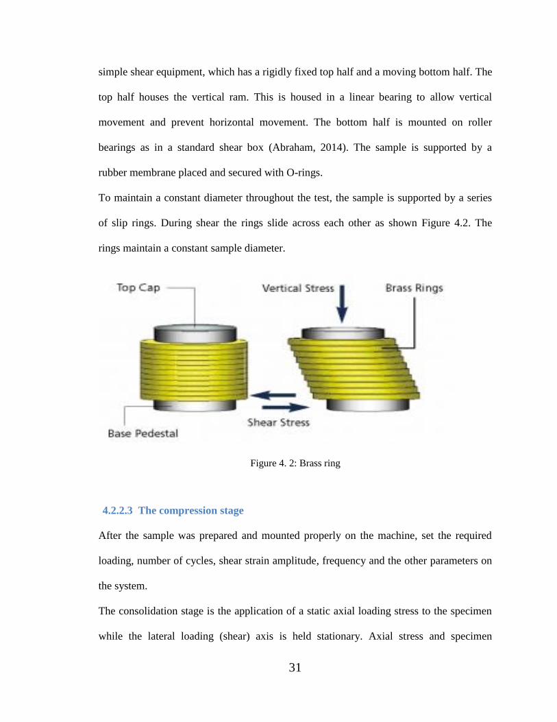
To maintain a constant diameter throughout the test, the sample is supported by a series
of slip rings. During shear the rings slide across each other as shown Figure 4.2. The
rings maintain a constant sample diameter.
Figure 4. 2: Brass ring
4.2.2.3 The compression stage
After the sample was prepared and mounted properly on the machine, set the required
loading, number of cycles, shear strain amplitude, frequency and the other parameters on
the system.
The consolidation stage is the application of a static axial loading stress to the specimen
while the lateral loading (shear) axis is held stationary. Axial stress and specimen
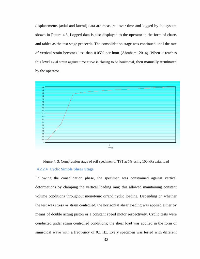
32
displacements (axial and lateral) data are measured over time and logged by the system
shown in Figure 4.3. Logged data is also displayed to the operator in the form of charts
and tables as the test stage proceeds. The consolidation stage was continued until the rate
of vertical strain becomes less than 0.05% per hour (Abraham, 2014). When it reaches
this level axial strain against time curve is closing to be horizontal, then manually terminated
by the operator.
Figure 4. 3: Compression stage of soil specimen of TP1 at 5% using 100 kPa axial load
4.2.2.4 Cyclic Simple Shear Stage
Following the consolidation phase, the specimen was constrained against vertical
deformations by clamping the vertical loading ram; this allowed maintaining constant
volume conditions throughout monotonic or/and cyclic loading. Depending on whether
the test was stress or strain controlled, the horizontal shear loading was applied either by
means of double acting piston or a constant speed motor respectively. Cyclic tests were
conducted under strain controlled conditions; the shear load was applied in the form of
sinusoidal wave with a frequency of 0.1 Hz. Every specimen was tested with different
Time (s)
10
Dis
pla
cem
ent (m
m)
0.38
0.36
0.34
0.32
0.3
0.28
0.26
0.24
0.22
0.2
0.18
0.16
0.14
0.12
0.1
0.08
0.06
0.04
0.02
0
33
cyclic shear stress amplitude, so preparations of specimens and testing have been done
for each strain level and axial load for all representative test pits (Abraham, 2014). Both
lateral force and specimen displacements are measured for each loading cycle. Measured
data is obtained from 50 points on the sample captured over a single cycle period
(UTS004 2003).
4.2.3 Presentation of Cyclic Shear Test results
4.2.3.1 Axial loads and Shear Strain Levels used
Applied shearing strain values on the cyclic simple shear machine in all series of tests
varied from 0.01% up to 5% with their respective different axial loads. In this study, axial
loads of 100 kPa, 250 kPa and 400 kPa were used (see Table 4.2).
Table 4. 2: Axial stress and shear strain values used for the study
Soil type
Sample type
Axial stress
( kPa)
Shear strain (%)
Silty
Clay soil
Undisturbed
100 0.01 0.1 1 2.5 5
250 0.01 0.1 1 2.5 5
400 0.01 0.1 1 2.5 5
Clayey
Silt soil
Undisturbed
100 0.01 0.1 1 2.5 5
250 0.01 0.1 1 2.5 5
400 0.01 0.1 1 2.5 5
4.2.3.2 Shear stress and strain parameters
For single cyclic loading, the cyclic simple shear test gives series of raw data at 50 data
points. Measured data can be displayed to the operator on Microsoft Excel spreadsheet.
34
Out of these data, Lateral Lvdt (specimen displacements) and Lateral force were used to
calculate the shear stress (τ) and shear strain (γ) values. Using the specimen height after
consolidation (< 20 mm) and its diameter, 70 mm, the shear stress and shear strain of the
specimen can be calculated based on the following equation.
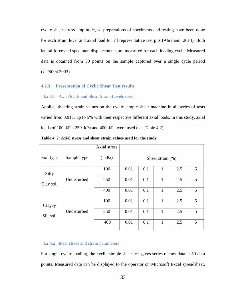
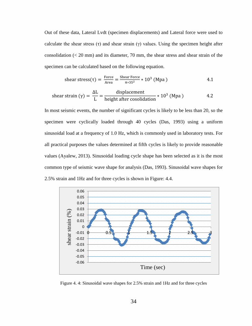
In most seismic events, the number of significant cycles is likely to be less than 20, so the
specimen were cyclically loaded through 40 cycles (Das, 1993) using a uniform
sinusoidal load at a frequency of 1.0 Hz, which is commonly used in laboratory tests. For
all practical purposes the values determined at fifth cycles is likely to provide reasonable
values (Ayalew, 2013). Sinusoidal loading cycle shape has been selected as it is the most
common type of seismic wave shape for analysis (Das, 1993). Sinusoidal wave shapes for
2.5% strain and 1Hz and for three cycles is shown in Figure: 4.4.
Figure 4. 4: Sinusoidal wave shapes for 2.5% strain and 1Hz and for three cycles
-0.06
-0.05
-0.04
-0.03
-0.02
-0.01
0
0.01
0.02
0.03
0.04
0.05
0.06
0 0.5 1 1.5 2 2.5 3
Time (sec)
shea
r st
rain
(%
)
35
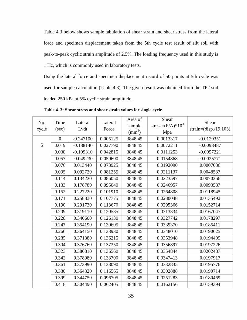
Table 4.3 below shows sample tabulation of shear strain and shear stress from the lateral
force and specimen displacement taken from the 5th cycle test result of silt soil with
peak-to-peak cyclic strain amplitude of 2.5%. The loading frequency used in this study is
1 Hz, which is commonly used in laboratory tests.
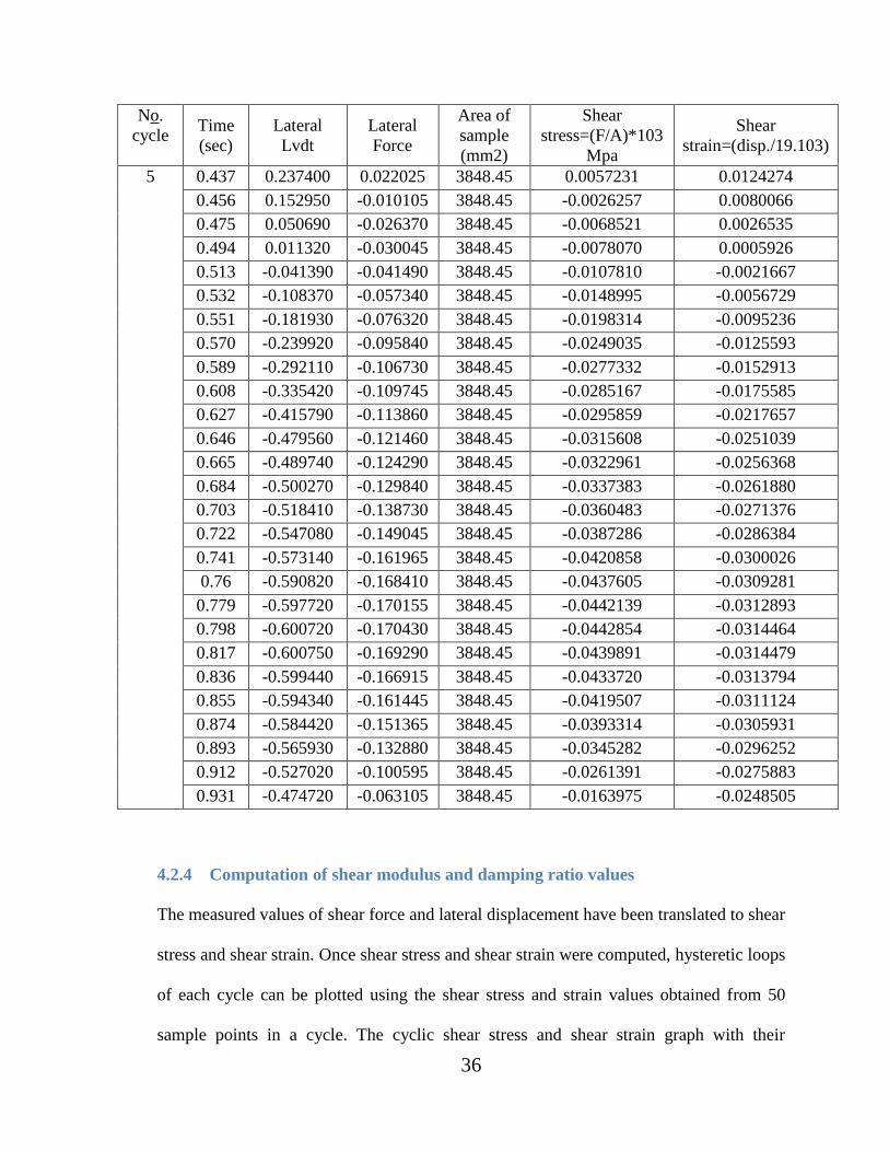
Using the lateral force and specimen displacement record of 50 points at 5th cycle was
used for sample calculation (Table 4.3). The given result was obtained from the TP2 soil
loaded 250 kPa at 5% cyclic strain amplitude.
Table 4. 3: Shear stress and shear strain values for single cycle.
No.
cycle
Time
(sec)
Lateral
Lvdt
Lateral
Force
Area of
sample
(mm2)
Shear
stress=(F/A)*103
Mpa
Shear
strain=(disp./19.103)
5
0 -0.247100 0.005125 3848.45 0.0013317 -0.0129351
0.019 -0.188140 0.027790 3848.45 0.0072211 -0.0098487
0.038 -0.109310 0.042815 3848.45 0.0111253 -0.0057221
0.057 -0.049230 0.059600 3848.45 0.0154868 -0.0025771
0.076 0.013440 0.073925 3848.45 0.0192090 0.0007036
0.095 0.092720 0.081255 3848.45 0.0211137 0.0048537
0.114 0.134230 0.086050 3848.45 0.0223597 0.0070266
0.133 0.178780 0.095040 3848.45 0.0246957 0.0093587
0.152 0.227220 0.101910 3848.45 0.0264808 0.0118945
0.171 0.258830 0.107775 3848.45 0.0280048 0.0135492
0.190 0.291730 0.113670 3848.45 0.0295366 0.0152714
0.209 0.319110 0.120585 3848.45 0.0313334 0.0167047
0.228 0.340600 0.126130 3848.45 0.0327742 0.0178297
0.247 0.354190 0.130605 3848.45 0.0339370 0.0185411
0.266 0.364150 0.133930 3848.45 0.0348010 0.0190625
0.285 0.371380 0.136215 3848.45 0.0353948 0.0194409
0.304 0.376760 0.137350 3848.45 0.0356897 0.0197226
0.323 0.386810 0.136560 3848.45 0.0354844 0.0202487
0.342 0.378080 0.133700 3848.45 0.0347413 0.0197917
0.361 0.373990 0.128090 3848.45 0.0332835 0.0195776
0.380 0.364320 0.116565 3848.45 0.0302888 0.0190714
0.399 0.344750 0.096705 3848.45 0.0251283 0.0180469
0.418 0.304490 0.062405 3848.45 0.0162156 0.0159394
36
No.
cycle Time
(sec)
Lateral
Lvdt
Lateral
Force
Area of
sample
(mm2)
Shear
stress=(F/A)*103
Mpa
Shear
strain=(disp./19.103)
5 0.437 0.237400 0.022025 3848.45 0.0057231 0.0124274
0.456 0.152950 -0.010105 3848.45 -0.0026257 0.0080066
0.475 0.050690 -0.026370 3848.45 -0.0068521 0.0026535
0.494 0.011320 -0.030045 3848.45 -0.0078070 0.0005926
0.513 -0.041390 -0.041490 3848.45 -0.0107810 -0.0021667
0.532 -0.108370 -0.057340 3848.45 -0.0148995 -0.0056729
0.551 -0.181930 -0.076320 3848.45 -0.0198314 -0.0095236
0.570 -0.239920 -0.095840 3848.45 -0.0249035 -0.0125593
0.589 -0.292110 -0.106730 3848.45 -0.0277332 -0.0152913
0.608 -0.335420 -0.109745 3848.45 -0.0285167 -0.0175585
0.627 -0.415790 -0.113860 3848.45 -0.0295859 -0.0217657
0.646 -0.479560 -0.121460 3848.45 -0.0315608 -0.0251039
0.665 -0.489740 -0.124290 3848.45 -0.0322961 -0.0256368
0.684 -0.500270 -0.129840 3848.45 -0.0337383 -0.0261880
0.703 -0.518410 -0.138730 3848.45 -0.0360483 -0.0271376
0.722 -0.547080 -0.149045 3848.45 -0.0387286 -0.0286384
0.741 -0.573140 -0.161965 3848.45 -0.0420858 -0.0300026
0.76 -0.590820 -0.168410 3848.45 -0.0437605 -0.0309281
0.779 -0.597720 -0.170155 3848.45 -0.0442139 -0.0312893
0.798 -0.600720 -0.170430 3848.45 -0.0442854 -0.0314464
0.817 -0.600750 -0.169290 3848.45 -0.0439891 -0.0314479
0.836 -0.599440 -0.166915 3848.45 -0.0433720 -0.0313794
0.855 -0.594340 -0.161445 3848.45 -0.0419507 -0.0311124
0.874 -0.584420 -0.151365 3848.45 -0.0393314 -0.0305931
0.893 -0.565930 -0.132880 3848.45 -0.0345282 -0.0296252
0.912 -0.527020 -0.100595 3848.45 -0.0261391 -0.0275883
0.931 -0.474720 -0.063105 3848.45 -0.0163975 -0.0248505
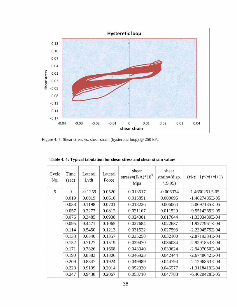
4.2.4 Computation of shear modulus and damping ratio values
The measured values of shear force and lateral displacement have been translated to shear
stress and shear strain. Once shear stress and shear strain were computed, hysteretic loops
of each cycle can be plotted using the shear stress and strain values obtained from 50
sample points in a cycle. The cyclic shear stress and shear strain graph with their
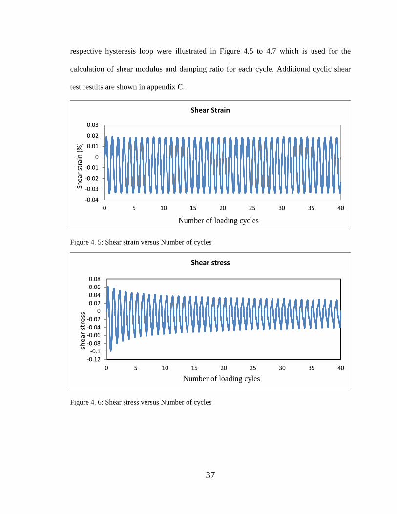
37
respective hysteresis loop were illustrated in Figure 4.5 to 4.7 which is used for the
calculation of shear modulus and damping ratio for each cycle. Additional cyclic shear
test results are shown in appendix C.
Figure 4. 5: Shear strain versus Number of cycles
Figure 4. 6: Shear stress versus Number of cycles
-0.04
-0.03
-0.02
-0.01
0
0.01
0.02
0.03
0 5 10 15 20 25 30 35 40
Shear Strain
Number of loading cycles
Shea
r st
rain
(%
)
-0.12-0.1
-0.08-0.06-0.04-0.02
00.020.040.060.08
0 5 10 15 20 25 30 35 40
Shear stress
Number of loading cyles
shea
r st
ress
38
Figure 4. 7: Shear stress vs. shear strain (hysteretic loop) @ 250 kPa
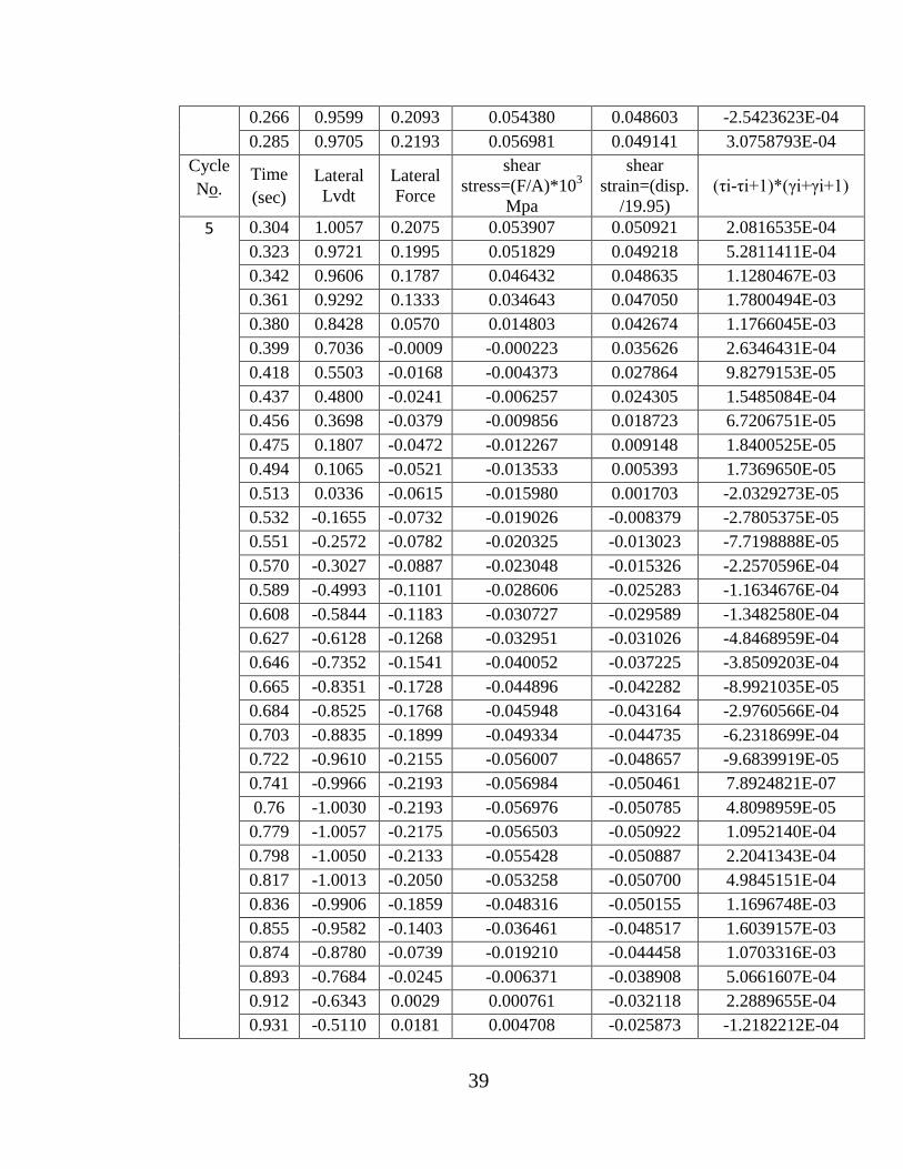
Table 4. 4: Typical tabulation for shear stress and shear strain values
Cycle
No.
Time
(sec)
Lateral
Lvdt
Lateral
Force
shear
stress=(F/A)*103
Mpa
shear
strain=(disp.
/19.95)
(τi-τi+1)*(γi+γi+1)
5 0 -0.1259 0.0520 0.013517 -0.006374 1.4650251E-05
0.019 0.0019 0.0610 0.015851 0.000095 -1.4627485E-05
0.038 0.1198 0.0701 0.018226 0.006064 -5.0697135E-05
0.057 0.2277 0.0812 0.021107 0.011529 -9.5514265E-05
0.076 0.3485 0.0938 0.024381 0.017644 -1.3303489E-04
0.095 0.4471 0.1065 0.027684 0.022637 -1.9277961E-04
0.114 0.5450 0.1213 0.031522 0.027593 -2.2304575E-04
0.133 0.6340 0.1357 0.035258 0.032100 -2.8719384E-04
0.152 0.7127 0.1519 0.039470 0.036084 -2.9291853E-04
0.171 0.7826 0.1668 0.043340 0.039624 -2.9407050E-04
0.190 0.8383 0.1806 0.046923 0.042444 -2.6748642E-04
0.209 0.8847 0.1924 0.049989 0.044794 -2.1296863E-04
0.228 0.9199 0.2014 0.052320 0.046577 -1.3118419E-04
0.247 0.9438 0.2067 0.053710 0.047788 -6.4620428E-05
-0.17
-0.14
-0.11
-0.08
-0.05
-0.02
0.01
0.04
0.07
0.10
0.13
-0.04 -0.03 -0.02 -0.01 0 0.01 0.02 0.03 0.04
She
ar s
tre
ss
shear strain
Hysteretic loop
39
0.266 0.9599 0.2093 0.054380 0.048603 -2.5423623E-04
0.285 0.9705 0.2193 0.056981 0.049141 3.0758793E-04
Cycle
No. Time
(sec)
Lateral
Lvdt
Lateral
Force
shear
stress=(F/A)*103
Mpa
shear
strain=(disp.
/19.95)
(τi-τi+1)*(γi+γi+1)
5 0.304 1.0057 0.2075 0.053907 0.050921 2.0816535E-04
0.323 0.9721 0.1995 0.051829 0.049218 5.2811411E-04
0.342 0.9606 0.1787 0.046432 0.048635 1.1280467E-03
0.361 0.9292 0.1333 0.034643 0.047050 1.7800494E-03
0.380 0.8428 0.0570 0.014803 0.042674 1.1766045E-03
0.399 0.7036 -0.0009 -0.000223 0.035626 2.6346431E-04
0.418 0.5503 -0.0168 -0.004373 0.027864 9.8279153E-05
0.437 0.4800 -0.0241 -0.006257 0.024305 1.5485084E-04
0.456 0.3698 -0.0379 -0.009856 0.018723 6.7206751E-05
0.475 0.1807 -0.0472 -0.012267 0.009148 1.8400525E-05
0.494 0.1065 -0.0521 -0.013533 0.005393 1.7369650E-05
0.513 0.0336 -0.0615 -0.015980 0.001703 -2.0329273E-05
0.532 -0.1655 -0.0732 -0.019026 -0.008379 -2.7805375E-05
0.551 -0.2572 -0.0782 -0.020325 -0.013023 -7.7198888E-05
0.570 -0.3027 -0.0887 -0.023048 -0.015326 -2.2570596E-04
0.589 -0.4993 -0.1101 -0.028606 -0.025283 -1.1634676E-04
0.608 -0.5844 -0.1183 -0.030727 -0.029589 -1.3482580E-04
0.627 -0.6128 -0.1268 -0.032951 -0.031026 -4.8468959E-04
0.646 -0.7352 -0.1541 -0.040052 -0.037225 -3.8509203E-04
0.665 -0.8351 -0.1728 -0.044896 -0.042282 -8.9921035E-05
0.684 -0.8525 -0.1768 -0.045948 -0.043164 -2.9760566E-04
0.703 -0.8835 -0.1899 -0.049334 -0.044735 -6.2318699E-04
0.722 -0.9610 -0.2155 -0.056007 -0.048657 -9.6839919E-05
0.741 -0.9966 -0.2193 -0.056984 -0.050461 7.8924821E-07
0.76 -1.0030 -0.2193 -0.056976 -0.050785 4.8098959E-05
0.779 -1.0057 -0.2175 -0.056503 -0.050922 1.0952140E-04
0.798 -1.0050 -0.2133 -0.055428 -0.050887 2.2041343E-04
0.817 -1.0013 -0.2050 -0.053258 -0.050700 4.9845151E-04
0.836 -0.9906 -0.1859 -0.048316 -0.050155 1.1696748E-03
0.855 -0.9582 -0.1403 -0.036461 -0.048517 1.6039157E-03
0.874 -0.8780 -0.0739 -0.019210 -0.044458 1.0703316E-03
0.893 -0.7684 -0.0245 -0.006371 -0.038908 5.0661607E-04
0.912 -0.6343 0.0029 0.000761 -0.032118 2.2889655E-04
0.931 -0.5110 0.0181 0.004708 -0.025873 -1.2182212E-04
40
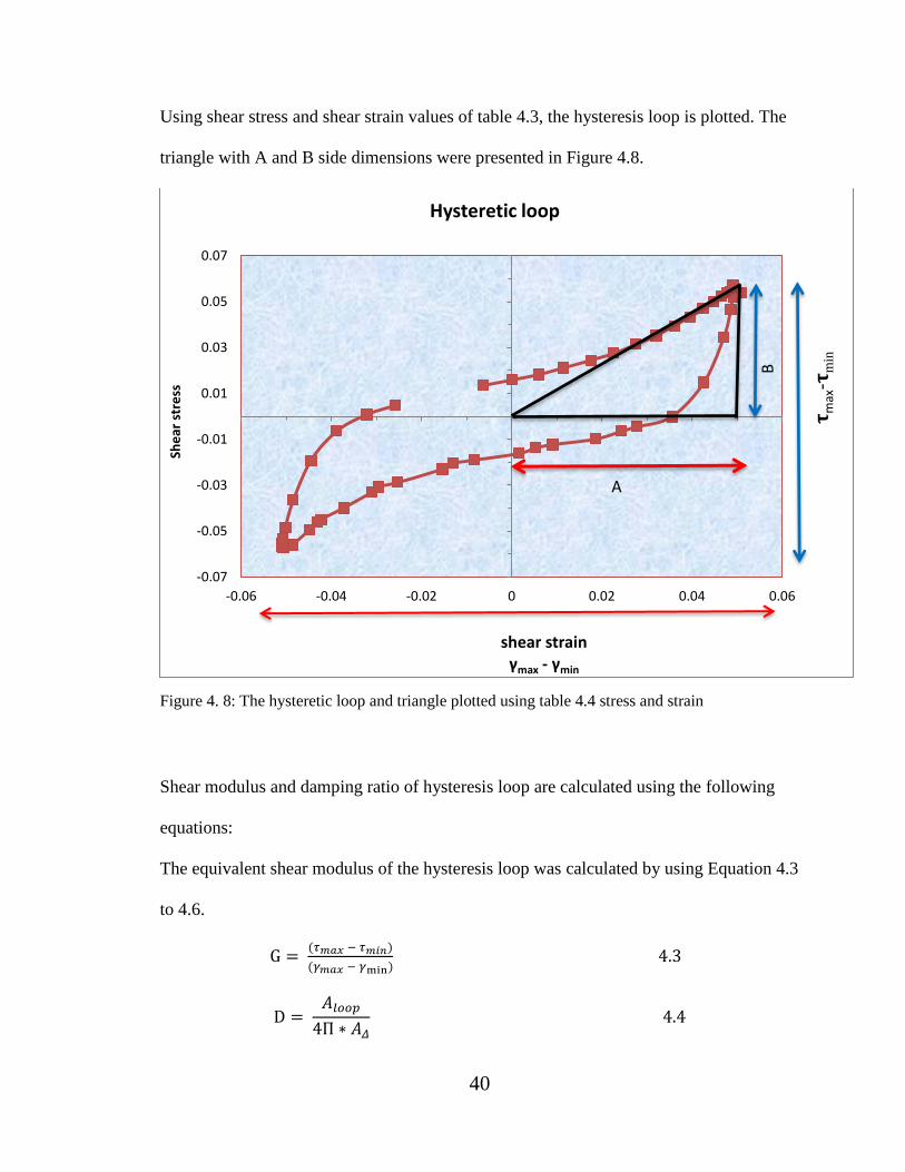
Using shear stress and shear strain values of table 4.3, the hysteresis loop is plotted. The
triangle with A and B side dimensions were presented in Figure 4.8.
Figure 4. 8: The hysteretic loop and triangle plotted using table 4.4 stress and strain
Shear modulus and damping ratio of hysteresis loop are calculated using the following
equations:
The equivalent shear modulus of the hysteresis loop was calculated by using Equation 4.3
to 4.6.
-0.07
-0.05
-0.03
-0.01
0.01
0.03
0.05
0.07
-0.06 -0.04 -0.02 0 0.02 0.04 0.06
She
ar s
tre
ss
shear strain γmax - γmin
Hysteretic loop
𝛕m
ax-𝛕
min
B
A
41
𝜏 𝜏 𝛾 𝛾
2A – The difference between the maximum and the minimum values of shear strain
2B - The difference between the maximum and the minimum values of shear stress
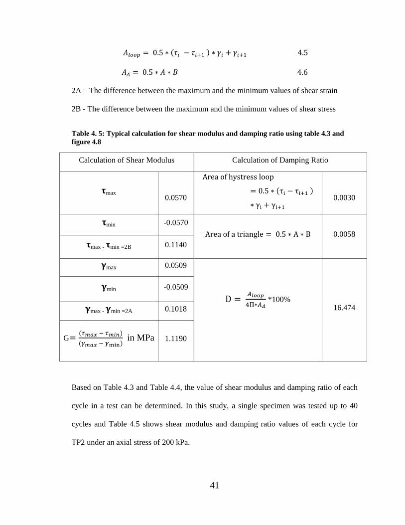
Table 4. 5: Typical calculation for shear modulus and damping ratio using table 4.3 and
figure 4.8
Calculation of Shear Modulus Calculation of Damping Ratio
𝞃max
0.0570
0.0030
𝞃min -0.0570
0.0058
𝞃max - 𝞃min =2B 0.1140
𝛄max 0.0509
*100%
16.474
𝛄min -0.0509
𝛄max - 𝛄min =2A 0.1018
G
in MPa 1.1190
Based on Table 4.3 and Table 4.4, the value of shear modulus and damping ratio of each
cycle in a test can be determined. In this study, a single specimen was tested up to 40
cycles and Table 4.5 shows shear modulus and damping ratio values of each cycle for
TP2 under an axial stress of 200 kPa.
42
Table 4. 6: Shear modulus and damping ratio values for TP2 under an axial stress of 250 kPa
Strain
level 0.01% 0.1% 1% 2.5% 5%
0.01
% 0.1% 1% 2.5% 5%
Cycle
No. G (MPa) D (%)
1 5.294 3.465 2.310 1.864 1.663 4.396 5.655 11.304 17.991 21.405
2 5.191 3.322 2.301 1.850 1.651 4.546 5.649 10.645 17.792 21.393
3 4.763 3.315 2.277 1.831 1.651 4.173 5.589 9.861 16.500 21.388
4 4.648 3.098 2.003 1.794 1.600 4.252 5.162 9.956 15.205 20.719
5 4.621 3.086 1.994 1.762 1.549 4.001 5.574 10.112 15.161 20.659
6 4.528 2.980 1.976 1.711 1.535 4.231 5.162 9.137 14.656 20.250
7 4.356 2.969 1.971 1.684 1.527 4.010 5.068 9.439 13.956 20.006
8 4.321 2.964 1.864 1.652 1.526 4.260 5.122 8.984 14.306 19.188
9 4.300 2.961 1.862 1.634 1.516 4.100 4.987 9.156 13.365 18.684
10 4.255 2.960 1.877 1.613 1.515 3.969 5.077 9.439 14.031 18.612
11 4.255 2.948 1.851 1.592 1.481 3.848 4.923 8.783 13.165 18.311
12 4.183 2.948 1.844 1.581 1.455 3.727 5.006 8.681 13.790 18.304
13 4.127 2.945 1.838 1.559 1.431 3.946 4.936 8.677 13.389 18.047
14 4.089 2.944 1.833 1.546 1.409 3.625 4.875 8.485 13.974 17.949
15 4.109 2.938 1.830 1.537 1.389 3.932 4.936 8.433 13.374 17.730
16 4.070 2.721 1.751 1.530 1.368 3.653 5.090 8.803 12.599 17.682
17 4.077 2.721 1.748 1.524 1.357 3.880 4.964 8.388 13.339 17.630
18 4.049 2.721 1.747 1.508 1.343 3.603 4.958 8.568 12.718 17.591
19 4.051 2.719 1.741 1.505 1.326 3.854 4.923 8.308 13.277 17.540
20 4.040 2.715 1.751 1.500 1.312 3.580 4.895 8.971 12.728 17.426
21 4.029 2.719 1.737 1.498 1.302 3.836 4.940 8.296 13.181 17.344
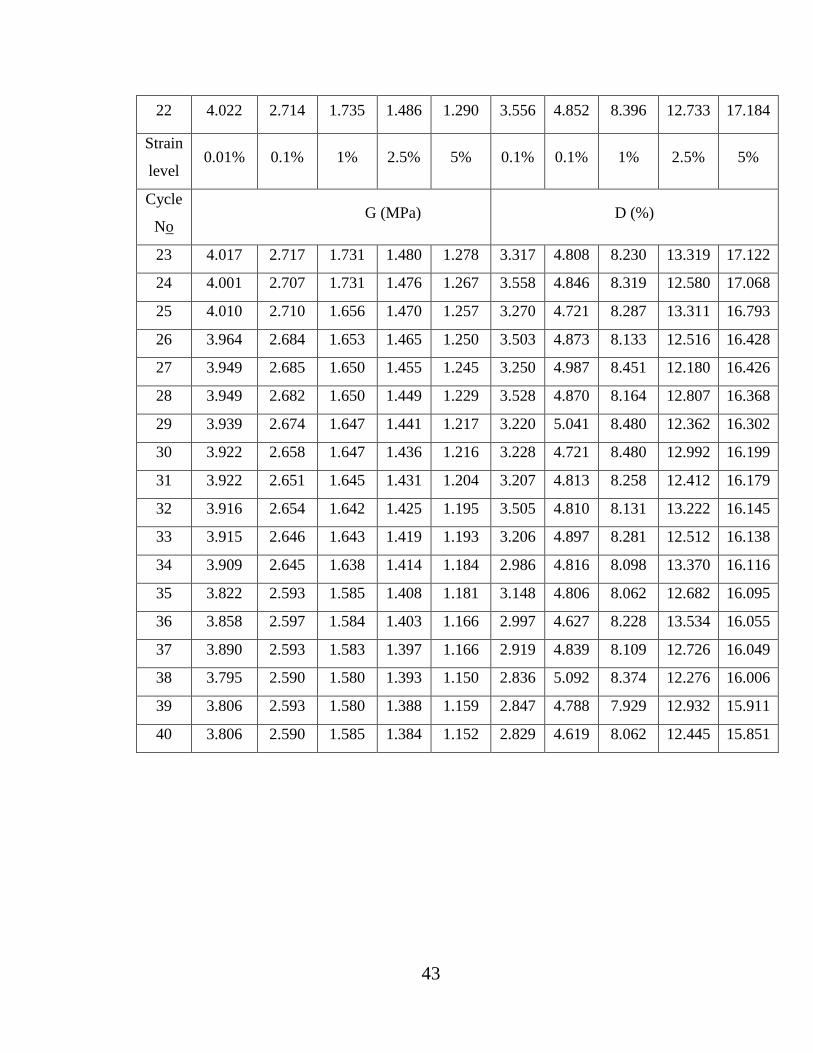
43
22 4.022 2.714 1.735 1.486 1.290 3.556 4.852 8.396 12.733 17.184
Strain
level 0.01% 0.1% 1% 2.5% 5% 0.1% 0.1% 1% 2.5% 5%
Cycle
No G (MPa) D (%)
23 4.017 2.717 1.731 1.480 1.278 3.317 4.808 8.230 13.319 17.122
24 4.001 2.707 1.731 1.476 1.267 3.558 4.846 8.319 12.580 17.068
25 4.010 2.710 1.656 1.470 1.257 3.270 4.721 8.287 13.311 16.793
26 3.964 2.684 1.653 1.465 1.250 3.503 4.873 8.133 12.516 16.428
27 3.949 2.685 1.650 1.455 1.245 3.250 4.987 8.451 12.180 16.426
28 3.949 2.682 1.650 1.449 1.229 3.528 4.870 8.164 12.807 16.368
29 3.939 2.674 1.647 1.441 1.217 3.220 5.041 8.480 12.362 16.302
30 3.922 2.658 1.647 1.436 1.216 3.228 4.721 8.480 12.992 16.199
31 3.922 2.651 1.645 1.431 1.204 3.207 4.813 8.258 12.412 16.179
32 3.916 2.654 1.642 1.425 1.195 3.505 4.810 8.131 13.222 16.145
33 3.915 2.646 1.643 1.419 1.193 3.206 4.897 8.281 12.512 16.138
34 3.909 2.645 1.638 1.414 1.184 2.986 4.816 8.098 13.370 16.116
35 3.822 2.593 1.585 1.408 1.181 3.148 4.806 8.062 12.682 16.095
36 3.858 2.597 1.584 1.403 1.166 2.997 4.627 8.228 13.534 16.055
37 3.890 2.593 1.583 1.397 1.166 2.919 4.839 8.109 12.726 16.049
38 3.795 2.590 1.580 1.393 1.150 2.836 5.092 8.374 12.276 16.006
39 3.806 2.593 1.580 1.388 1.159 2.847 4.788 7.929 12.932 15.911
40 3.806 2.590 1.585 1.384 1.152 2.829 4.619 8.062 12.445 15.851
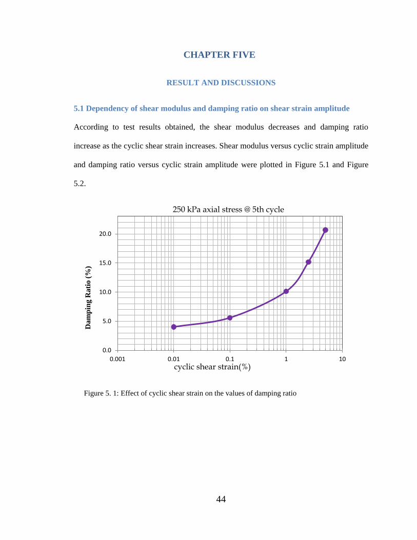
44
CHAPTER FIVE
RESULT AND DISCUSSIONS
5.1 Dependency of shear modulus and damping ratio on shear strain amplitude
According to test results obtained, the shear modulus decreases and damping ratio
increase as the cyclic shear strain increases. Shear modulus versus cyclic strain amplitude
and damping ratio versus cyclic strain amplitude were plotted in Figure 5.1 and Figure
5.2.
Figure 5. 1: Effect of cyclic shear strain on the values of damping ratio
0.0
5.0
10.0
15.0
20.0
0.001 0.01 0.1 1 10
250 kPa axial stress @ 5th cycle
cyclic shear strain(%)
Da
mp
ing
Ra
tio
(%
)
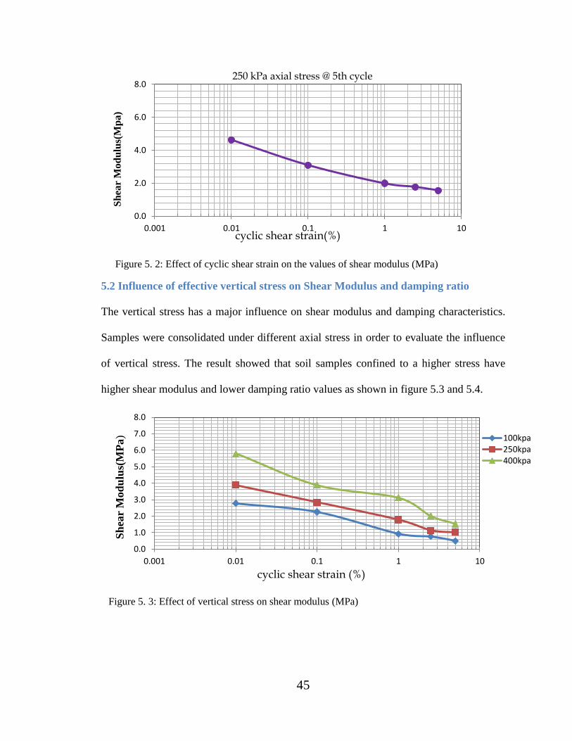
45
Figure 5. 2: Effect of cyclic shear strain on the values of shear modulus (MPa)
5.2 Influence of effective vertical stress on Shear Modulus and damping ratio
The vertical stress has a major influence on shear modulus and damping characteristics.
Samples were consolidated under different axial stress in order to evaluate the influence
of vertical stress. The result showed that soil samples confined to a higher stress have
higher shear modulus and lower damping ratio values as shown in figure 5.3 and 5.4.
Figure 5. 3: Effect of vertical stress on shear modulus (MPa)
0.0
2.0
4.0
6.0
8.0
0.001 0.01 0.1 1 10
250 kPa axial stress @ 5th cycle
cyclic shear strain(%)
Sh
ear M
od
ulu
s(M
pa
)
0.0
1.0
2.0
3.0
4.0
5.0
6.0
7.0
8.0
0.001 0.01 0.1 1 10
100kpa250kpa400kpa
cyclic shear strain (%)
Sh
ear
Mod
ulu
s(M
Pa
)
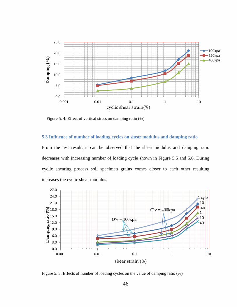
46
Figure 5. 4: Effect of vertical stress on damping ratio (%)
5.3 Influence of number of loading cycles on shear modulus and damping ratio
From the test result, it can be observed that the shear modulus and damping ratio
decreases with increasing number of loading cycle shown in Figure 5.5 and 5.6. During
cyclic shearing process soil specimen grains comes closer to each other resulting
increases the cyclic shear modulus.
Figure 5. 5: Effects of number of loading cycles on the value of damping ratio (%)
0.0
5.0
10.0
15.0
20.0
25.0
0.001 0.01 0.1 1 10
100kpa250kpa400kpa
cyclic shear strain(%)
Dam
pin
g (
%)
0.0
3.0
6.0
9.0
12.0
15.0
18.0
21.0
24.0
27.0
0.001 0.01 0.1 1 10
1 cyle 10 40
shear strain (%)
Da
mp
ing
ra
tio
(%
)
1 10 40
σ'v = 100kpa
σ'v = 400kpa
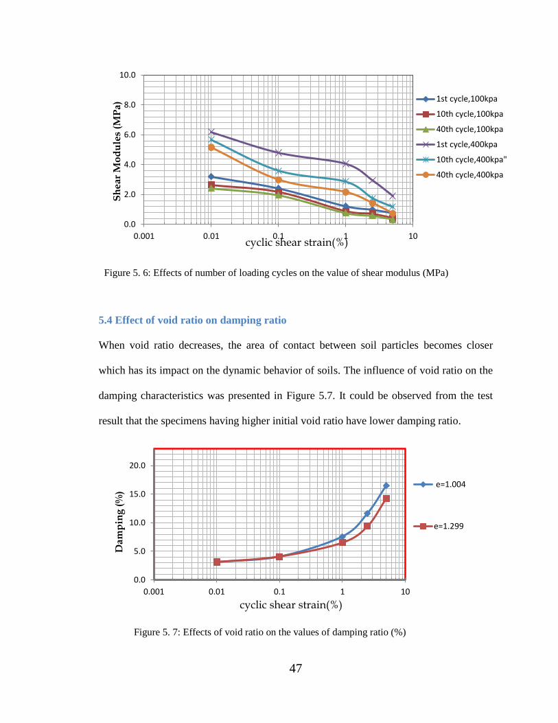
47
Figure 5. 6: Effects of number of loading cycles on the value of shear modulus (MPa)
5.4 Effect of void ratio on damping ratio
When void ratio decreases, the area of contact between soil particles becomes closer
which has its impact on the dynamic behavior of soils. The influence of void ratio on the
damping characteristics was presented in Figure 5.7. It could be observed from the test
result that the specimens having higher initial void ratio have lower damping ratio.
Figure 5. 7: Effects of void ratio on the values of damping ratio (%)
0.0
2.0
4.0
6.0
8.0
10.0
0.001 0.01 0.1 1 10
1st cycle,100kpa
10th cycle,100kpa
40th cycle,100kpa
1st cycle,400kpa
10th cycle,400kpa"
40th cycle,400kpa
cyclic shear strain(%)
Sh
ea
r M
od
ule
s (M
Pa
)
0.0
5.0
10.0
15.0
20.0
0.001 0.01 0.1 1 10
e=1.004
e=1.299
cyclic shear strain(%)
Da
mp
ing
(%
)
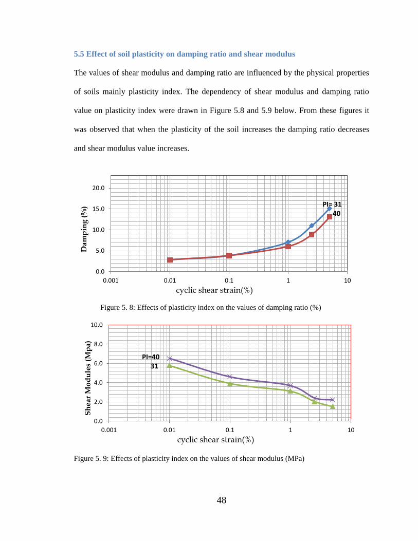
48
5.5 Effect of soil plasticity on damping ratio and shear modulus
The values of shear modulus and damping ratio are influenced by the physical properties
of soils mainly plasticity index. The dependency of shear modulus and damping ratio
value on plasticity index were drawn in Figure 5.8 and 5.9 below. From these figures it
was observed that when the plasticity of the soil increases the damping ratio decreases
and shear modulus value increases.
Figure 5. 8: Effects of plasticity index on the values of damping ratio (%)
Figure 5. 9: Effects of plasticity index on the values of shear modulus (MPa)
0.0
5.0
10.0
15.0
20.0
0.001 0.01 0.1 1 10
cyclic shear strain(%)
Dam
pin
g (
%) PI= 31
40
0.0
2.0
4.0
6.0
8.0
10.0
0.001 0.01 0.1 1 10
cyclic shear strain(%)
Sh
ea
r M
od
ule
s (M
pa)
PI=40 31
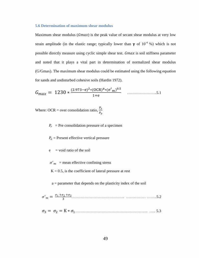
49
5.6 Determination of maximum shear modulus
Maximum shear modulus (𝐺𝑚𝑎𝑥) is the peak value of secant shear modulus at very low
strain amplitude (in the elastic range; typically lower than 𝛄 of 10-4
%) which is not
possible directly measure using cyclic simple shear test. 𝐺𝑚𝑎𝑥 is soil stiffness parameter
and noted that it plays a vital part in determination of normalized shear modulus
(G/Gmax). The maximum shear modulus could be estimated using the following equation
for sands and undisturbed cohesive soils (Hardin 1972).
𝐺
…………………..5.1
Where: OCR = over consolidation ratio,
= Pre consolidation pressure of a specimen
= Present effective vertical pressure
e = void ratio of the soil
= mean effective confining stress
K = 0.5, is the coefficient of lateral pressure at rest
a = parameter that depends on the plasticity index of the soil
………………………………….. …………… ……..5.2
……………………………………………….. ….. 5.3
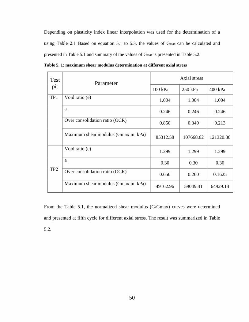
50
Depending on plasticity index linear interpolation was used for the determination of a
using Table 2.1 Based on equation 5.1 to 5.3, the values of Gmax can be calculated and
presented in Table 5.1 and summary of the values of Gmax is presented in Table 5.2.
Table 5. 1: maximum shear modulus determination at different axial stress
Test
pit Parameter
Axial stress
100 kPa 250 kPa 400 kPa
TP1 Void ratio (e) 1.004 1.004 1.004
a 0.246 0.246 0.246
Over consolidation ratio (OCR) 0.850 0.340 0.213
Maximum shear modulus (Gmax in kPa)
85312.58
107668.62 121320.86
TP2
Void ratio (e) 1.299 1.299 1.299
a 0.30 0.30 0.30
Over consolidation ratio (OCR) 0.650 0.260 0.1625
Maximum shear modulus (Gmax in kPa) 49162.96 59049.41 64929.14
From the Table 5.1, the normalized shear modulus (G/Gmax) curves were determined
and presented at fifth cycle for different axial stress. The result was summarized in Table
5.2.
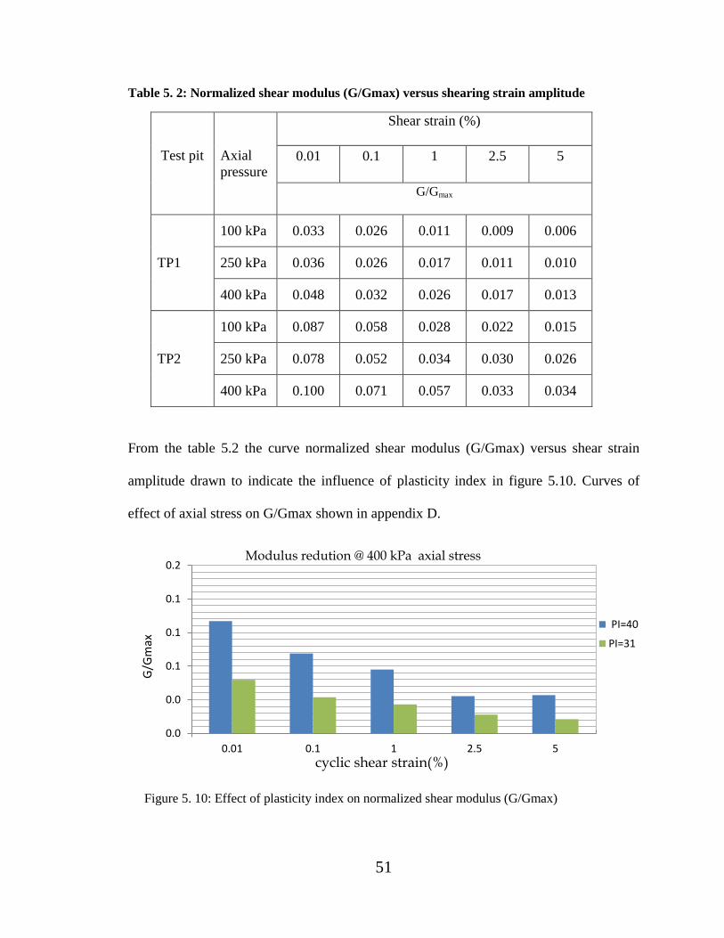
51
Table 5. 2: Normalized shear modulus (G/Gmax) versus shearing strain amplitude
Test pit Axial
pressure
Shear strain (%)
0.01 0.1 1 2.5 5
G/Gmax
TP1
100 kPa 0.033 0.026 0.011 0.009 0.006
250 kPa 0.036 0.026 0.017 0.011 0.010
400 kPa 0.048 0.032 0.026 0.017 0.013
TP2
100 kPa 0.087 0.058 0.028 0.022 0.015
250 kPa 0.078 0.052 0.034 0.030 0.026
400 kPa 0.100 0.071 0.057 0.033 0.034
From the table 5.2 the curve normalized shear modulus (G/Gmax) versus shear strain
amplitude drawn to indicate the influence of plasticity index in figure 5.10. Curves of
effect of axial stress on G/Gmax shown in appendix D.
Figure 5. 10: Effect of plasticity index on normalized shear modulus (G/Gmax)
0.0
0.0
0.1
0.1
0.1
0.2
0.01 0.1 1 2.5 5
PI=40
PI=31
cyclic shear strain(%)
G/G
max
Modulus redution @ 400 kPa axial stress
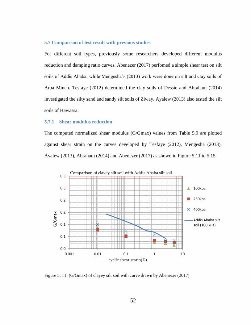
52
5.7 Comparison of test result with previous studies
For different soil types, previously some researchers developed different modulus
reduction and damping ratio curves. Abenezer (2017) perfomed a simple shear test on silt
soils of Addis Ababa, while Mengesha’s (2013) work were done on silt and clay soils of
Arba Minch. Tesfaye (2012) determined the clay soils of Dessie and Abraham (2014)
investigated the silty sand and sandy silt soils of Ziway. Ayalew (2013) also tasted the silt
soils of Hawassa.
5.7.1 Shear modulus reduction
The computed normalized shear modulus (G/Gmax) values from Table 5.9 are plotted
against shear strain on the curves developed by Tesfaye (2012), Mengesha (2013),
Ayalew (2013), Abraham (2014) and Abenezer (2017) as shown in Figure 5.11 to 5.15.
Figure 5. 11: (G/Gmax) of clayey silt soil with curve drawn by Abenezer (2017)
0.0
0.1
0.1
0.2
0.2
0.3
0.3
0.001 0.01 0.1 1 10
100kpa
250kpa
400kpa
Addis Ababa siltsoil (100 kPa)
cyclic shear strain(%)
G/G
max
Comparison of clayey silt soil with Addis Ababa silt soil
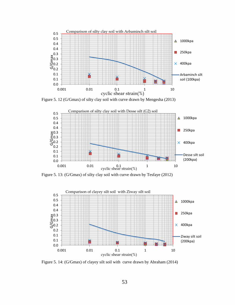
53
Figure 5. 12 (G/Gmax) of silty clay soil with curve drawn by Mengesha (2013)
Figure 5. 13: (G/Gmax) of silty clay soil with curve drawn by Tesfaye (2012)
Figure 5. 14: (G/Gmax) of clayey silt soil with curve drawn by Abraham (2014)
0.0
0.1
0.1
0.2
0.2
0.3
0.3
0.4
0.4
0.5
0.5
0.001 0.01 0.1 1 10
1000kpa
250kpa
400kpa
Arbaminch siltsoil (100kpa)
cyclic shear strain(%)
G/G
max
Comparison of silty clay soil with Arbaminch silt soil
0.00.10.10.20.20.30.30.40.40.50.5
0.001 0.01 0.1 1 10
1000kpa
250kpa
400kpa
Desse silt soil(200kpa)
cyclic shear strain(%)
G/G
max
Comparison of silty clay soil with Desse silt (G2) soil
0.0
0.1
0.1
0.2
0.2
0.3
0.3
0.4
0.4
0.5
0.5
0.001 0.01 0.1 1 10
1000kpa
250kpa
400kpa
Ziway silt soil(200kpa)
cyclic shear strain(%)
G/G
max
Comparison of clayey silt soil with Ziway silt soil
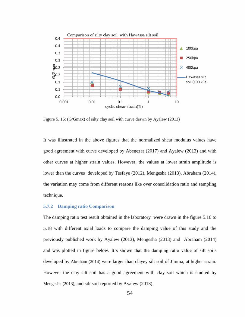
54
Figure 5. 15: (G/Gmax) of silty clay soil with curve drawn by Ayalew (2013)
It was illustrated in the above figures that the normalized shear modulus values have
good agreement with curve developed by Abenezer (2017) and Ayalew (2013) and with
other curves at higher strain values. However, the values at lower strain amplitude is
lower than the curves developed by Tesfaye (2012), Mengesha (2013), Abraham (2014),
the variation may come from different reasons like over consolidation ratio and sampling
technique.
5.7.2 Damping ratio Comparison
The damping ratio test result obtained in the laboratory were drawn in the figure 5.16 to
5.18 with different axial loads to compare the damping value of this study and the
previously published work by Ayalew (2013), Mengesha (2013) and Abraham (2014)
and was plotted in figure below. It’s shown that the damping ratio value of silt soils
developed by Abraham (2014) were larger than clayey silt soil of Jimma, at higher strain.
However the clay silt soil has a good agreement with clay soil which is studied by
Mengesha (2013), and silt soil reported by Ayalew (2013).
0.0
0.1
0.1
0.2
0.2
0.3
0.3
0.4
0.4
0.001 0.01 0.1 1 10
100kpa
250kpa
400kpa
Hawassa siltsoil (100 kPa)
cyclic shear strain(%)
G/G
max
Comparison of silty clay soil with Hawassa silt soil
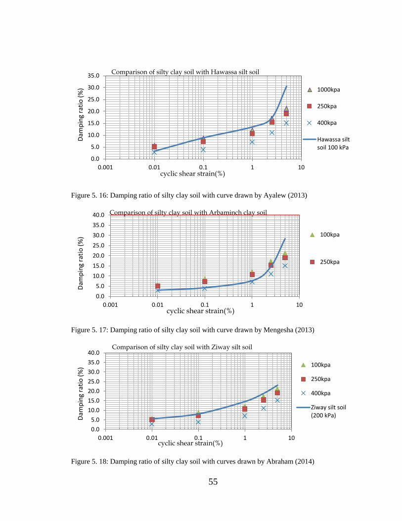
55
Figure 5. 16: Damping ratio of silty clay soil with curve drawn by Ayalew (2013)
Figure 5. 17: Damping ratio of silty clay soil with curve drawn by Mengesha (2013)
Figure 5. 18: Damping ratio of silty clay soil with curves drawn by Abraham (2014)
0.0
5.0
10.0
15.0
20.0
25.0
30.0
35.0
0.001 0.01 0.1 1 10
1000kpa
250kpa
400kpa
Hawassa siltsoil 100 kPa
cyclic shear strain(%)
Dam
pin
g ra
tio
(%
) Comparison of silty clay soil with Hawassa silt soil
0.0
5.0
10.0
15.0
20.0
25.0
30.0
35.0
40.0
0.001 0.01 0.1 1 10
100kpa
250kpa
cyclic shear strain(%)
Dam
pin
g ra
tio
(%
)
Comparison of silty clay soil with Arbaminch clay soil
0.0
5.0
10.0
15.0
20.0
25.0
30.0
35.0
40.0
0.001 0.01 0.1 1 10
100kpa
250kpa
400kpa
Ziway silt soil(200 kPa)
cyclic shear strain(%)
Dam
pin
g ra
tio
(%
)
Comparison of silty clay soil with Ziway silt soil
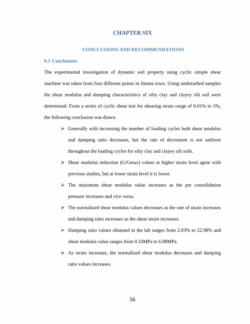
56
CHAPTER SIX
CONCLUSIONS AND RECOMMENDATIONS
6.1 Conclusions
The experimental investigation of dynamic soil property using cyclic simple shear
machine was taken from four different points in Jimma town. Using undisturbed samples
the shear modulus and damping characteristics of silty clay and clayey silt soil were
determined. From a series of cyclic shear test for shearing strain range of 0.01% to 5%,
the following conclusion was drawn.
Generally with increasing the number of loading cycles both shear modulus
and damping ratio decreases, but the rate of decrement is not uniform
throughout the loading cycles for silty clay and clayey silt soils.
Shear modulus reduction (G/Gmax) values at higher strain level agree with
previous studies, but at lower strain level it is lower.
The maximum shear modulus value increases as the pre consolidation
pressure increases and vice versa.
The normalized shear modulus values decreases as the rate of strain increases
and damping ratio increases as the shear strain increases.
Damping ratio values obtained in the lab ranges from 2.03% to 22.98% and
shear modulus value ranges from 0.33MPa to 6.98MPa.
As strain increases, the normalized shear modulus decreases and damping
ratio values increases.
57
6.2 Recommendations for Future work
The results obtained from this research study provide some basic insights
about normalized shear modulus and damping characteristics of soil in
Jimma town.
More data on modulus and damping on the soil from various locations using
different testing equipment would help to construct more accurate specific
modulus reduction and damping curves for silty clay and clayey silt soil of
Jimma town.
Tests using cyclic triaxial and resonant column devices would provide
additional information regarding the influence of loading mode, anisotropy
and principal stress rotation on monotonic and cyclic strength of soil.
Investigation to a very deep sub surface profile using some drilling equipment
can also give the depth effect of dynamic soil parameters.
58
REFERENCES
Abenezer T.,“Investigation of the Damping Ratio and Shear Modulus of Soil along Light
Rail Transit Route in Megenagna-Hayat Road,” International Journal of Scientific &
Engineering Research, 2017, v 8, pp.111-122.
Aberham Mengistu, “Investigation in to some dynamic properties of soils around ziway”,
Addis Ababa University,2014.
Abu Gemechu,” Shear modulus and Damping ratio values of soils found in Adama”,
Addis Ababa University, 2011.
ASTM, “American society for testing and materials”, Annual Book of ASTM
Standards,1998
Ayalew Gashaw, “Shear modulus and Damping ratio values of soils found in Adama “,
Addis Ababa University, 2013.
Boonam Shin,” Effects of Oversized Particles on the Dynamic Properties of Sand
Specimens Evaluated by Resonant Column Testing, Austin” University of Texas, 2014.
Das, B.M., “Principles of Soil Dynamics”, California State University, Scramento:, 1993.
David Umberg,” Dynamic Properties of Soils with Non-Plastic Fines,” Austin: University
of Texas, 2012
Girmachew Yimer,” shear modulus and Damping Ratio of Dry Koka Sand Cyclic Simple
Shear Test”, Addis Ababa University, 2010
Hardin, B. O. and V. P. Drnevich, "Shear Modulus and Damping in Soils: Design
Equations and Curves." Journal of the Soil Mechanics and Foundations Division, ASCE,
1972 Vol. 98, No.SM7, pp. 667-692.
H. Bolton Seed, Robert T. Wong, I.M Idriss and K. Tokimatsu, University of California.
Moduli and Factors for Dynamic Analyses of Cohesionless Soils, 1984.
Kakusho, T.,“Cyclic triaxial test of Dynamic soil properties for wide strain ranges,"
Central Research Institute of Electric Power Industry, 1979, pp.305-312.
Kramer S.I., “Geotechnical Earthquake Engineering,” University of Washington,
Prentice-Hall Inc., United States of America,1996
Luna, R., and Jadi, H.,“Determination of dynamic soil properties using Geophsical
methods,” Department of Civil Engineering, University of Missouri-Rolla, 2000.
59
MengeshaTefera, Tadiwos Chernet and Workineh Haro,”Geological Survey of Ethiopia,”
Regional Geology Department EIGS, 1996.
Muge K.,” Dynamic soil characterization and site response estimation for Erbaa, Tokat
(Turkey,” Ankara: Middle East Technical University, 2016.
Priyanka Sharma,” Effect of saturation on dynamic properties of Solani sanD,” Indian
Geotechnical Conference, 2016, pp.01- 05.
Seed, H.B. and Idriss, I.M., “Soil Moduli and Damping factors for dynamic response
analyses”, EERC/70-10, College of Engineering university of California, Berkeley, 1970
Sentheepan Thirugnanasampanther,”Cyclic behaviour and dynamic properties of soils
under simple shear loading,” University of East London, 2012.
Shankar S.,” Parameters Influencing dynamic Soil Properties,” nternational Journal of
Innovative Research in Science, Engineering and Technology.,2013, v 03, pp.47-60.
Soheil Moayerian,” Effect of Loading Frequency on Dynamic Properties of Soils Using
Resonant Column,” Canada: university of waterloo, 2012.
Tesfaye, Alemnew, “Index Properties, Shear Strength and Dynamic Properties of Soils
Found in Dessie,” Addis Ababa University, 2012.
T. G. Sitharam,” Dynamic Properties of Dry Sands,” Indian Geotechnical Journal, 2008,
v 38, pp.334-344.
UTS004, “Simple shear test software reference”, Universal testing system, IPC Global
limited, 2003
Vucetic and Dobry, “Soil Dynamics and Earth Quake Engineering”, 199.
Yamamuro, J. A. and Lade, P. V, “Steady-State Concepts and Static Liquefaction of Silty
Sands,” Journal of Geotechnical and Geo-environmental Engineering,1998 Vol. 124, pp.
868-87.
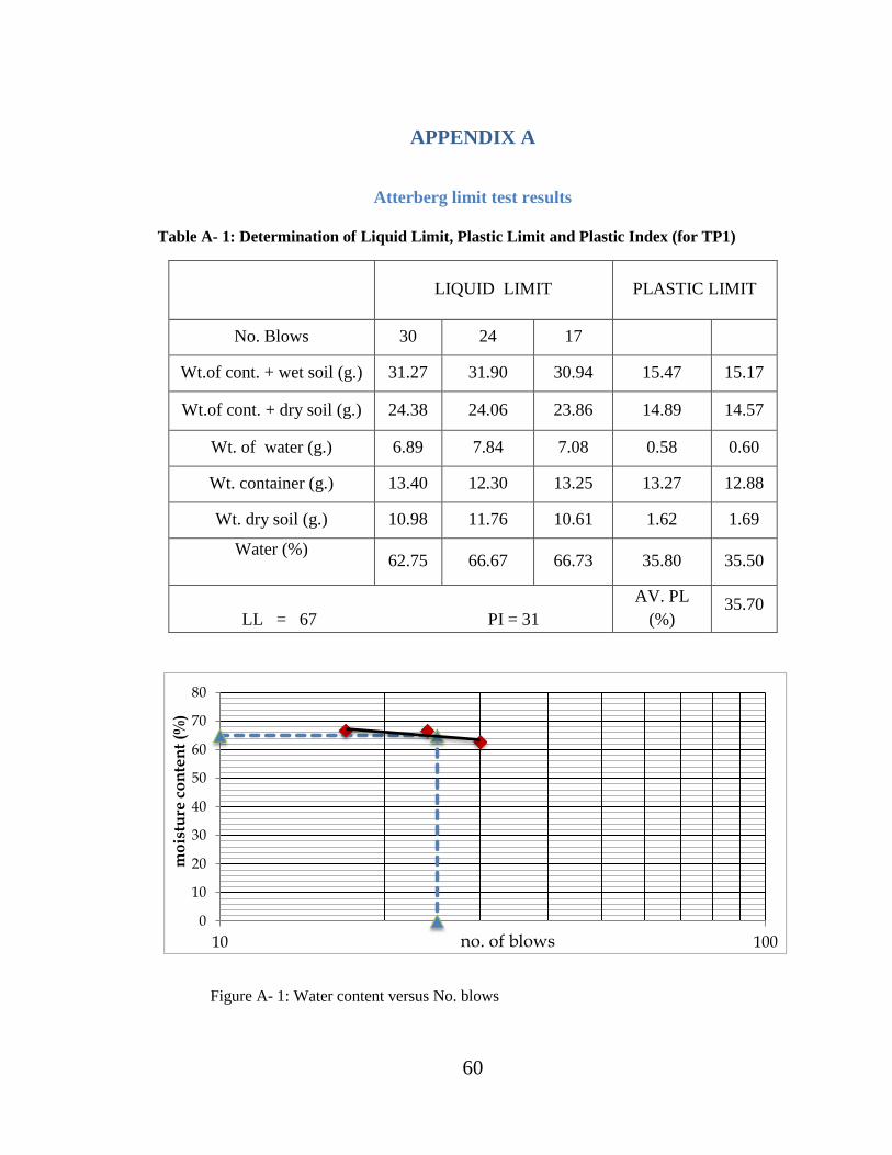
60
APPENDIX A
Atterberg limit test results
Table A- 1: Determination of Liquid Limit, Plastic Limit and Plastic Index (for TP1)
LIQUID LIMIT PLASTIC LIMIT
No. Blows 30 24 17
Wt.of cont. + wet soil (g.) 31.27 31.90 30.94 15.47 15.17
Wt.of cont. + dry soil (g.) 24.38 24.06 23.86 14.89 14.57
Wt. of water (g.) 6.89 7.84 7.08 0.58 0.60
Wt. container (g.) 13.40 12.30 13.25 13.27 12.88
Wt. dry soil (g.) 10.98 11.76 10.61 1.62 1.69
Water (%)
62.75 66.67 66.73 35.80 35.50
LL = 67 PI = 31
AV. PL
(%) 35.70
Figure A- 1: Water content versus No. blows
0
10
20
30
40
50
60
70
80
10 100no. of blows
mo
istu
re c
on
ten
t (%
)
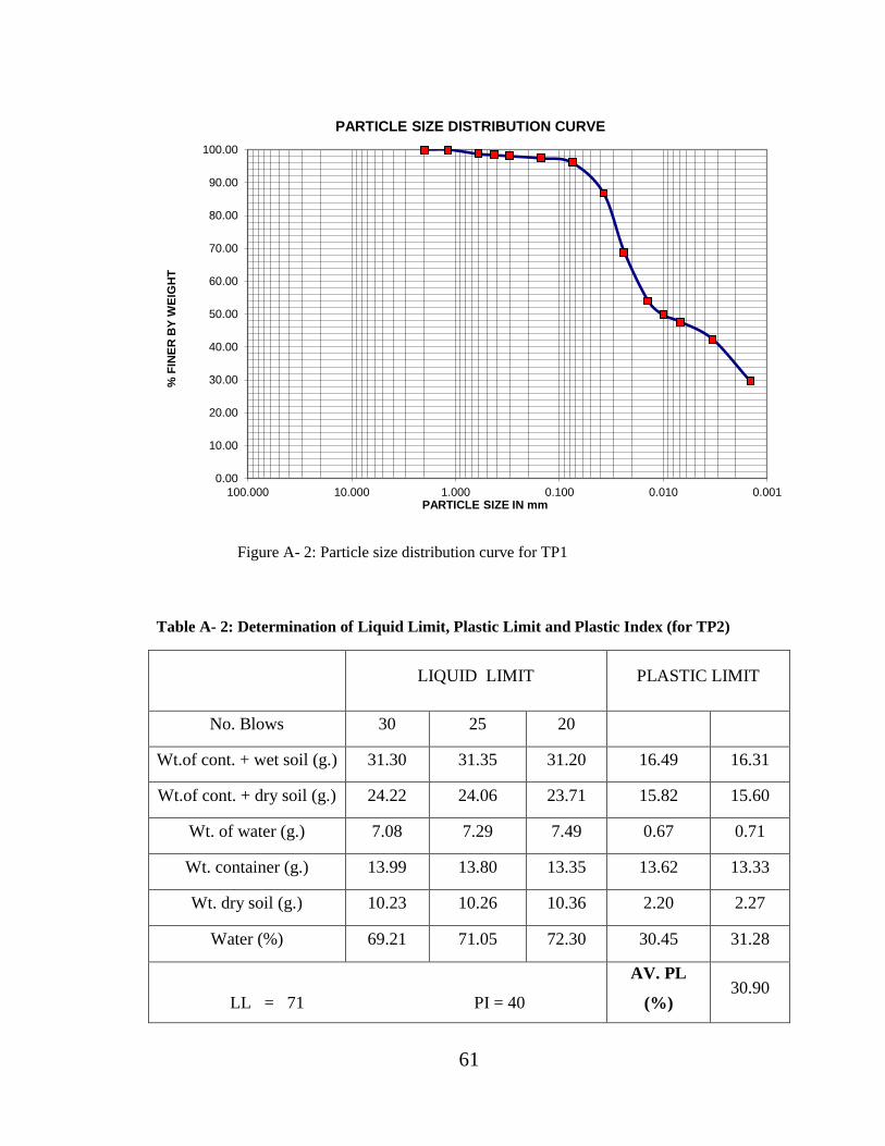
61
Figure A- 2: Particle size distribution curve for TP1
Table A- 2: Determination of Liquid Limit, Plastic Limit and Plastic Index (for TP2)
LIQUID LIMIT PLASTIC LIMIT
No. Blows 30 25 20
Wt.of cont. + wet soil (g.) 31.30 31.35 31.20 16.49 16.31
Wt.of cont. + dry soil (g.) 24.22 24.06 23.71 15.82 15.60
Wt. of water (g.) 7.08 7.29 7.49 0.67 0.71
Wt. container (g.) 13.99 13.80 13.35 13.62 13.33
Wt. dry soil (g.) 10.23 10.26 10.36 2.20 2.27
Water (%) 69.21 71.05 72.30 30.45 31.28
LL = 71 PI = 40
AV. PL
(%) 30.90
0.00
10.00
20.00
30.00
40.00
50.00
60.00
70.00
80.00
90.00
100.00
0.0010.0100.1001.00010.000100.000
% F
INE
R B
Y W
EIG
HT
PARTICLE SIZE IN mm
PARTICLE SIZE DISTRIBUTION CURVE
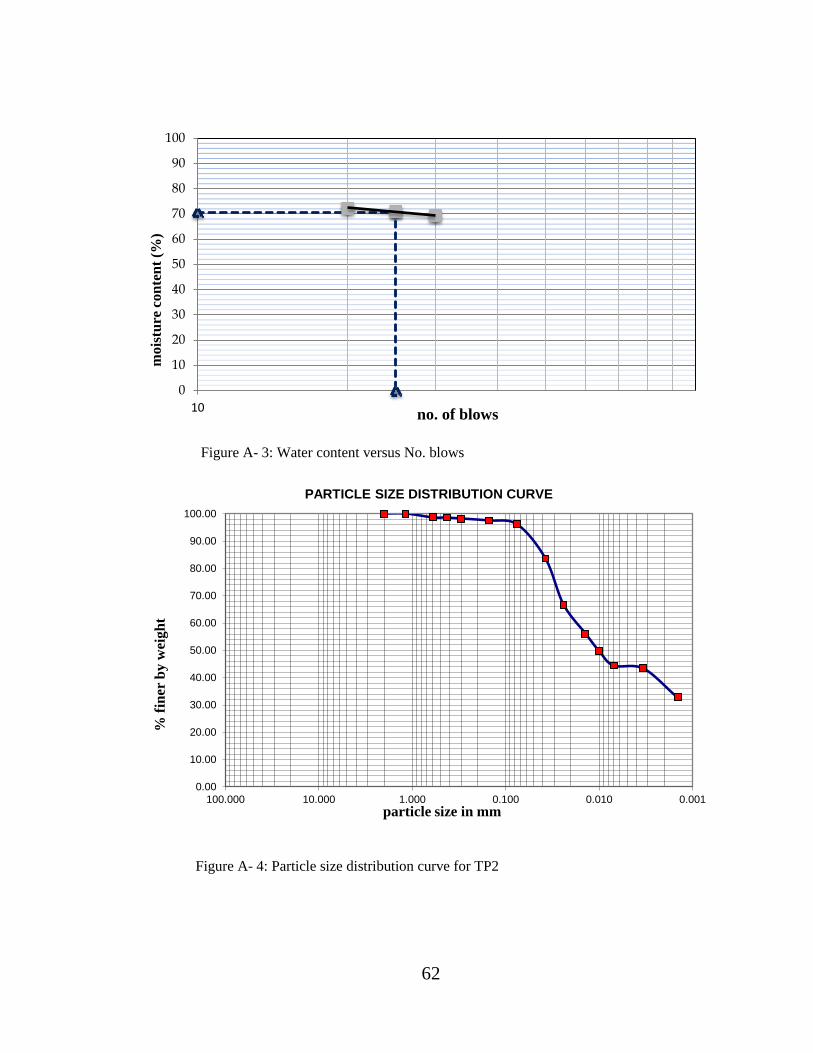
62
Figure A- 3: Water content versus No. blows
Figure A- 4: Particle size distribution curve for TP2
0
10
20
30
40
50
60
70
80
90
100
10
mo
istu
re c
on
ten
t (%
)
no. of blows
0.00
10.00
20.00
30.00
40.00
50.00
60.00
70.00
80.00
90.00
100.00
0.0010.0100.1001.00010.000100.000
% f
iner
by w
eig
ht
particle size in mm
PARTICLE SIZE DISTRIBUTION CURVE
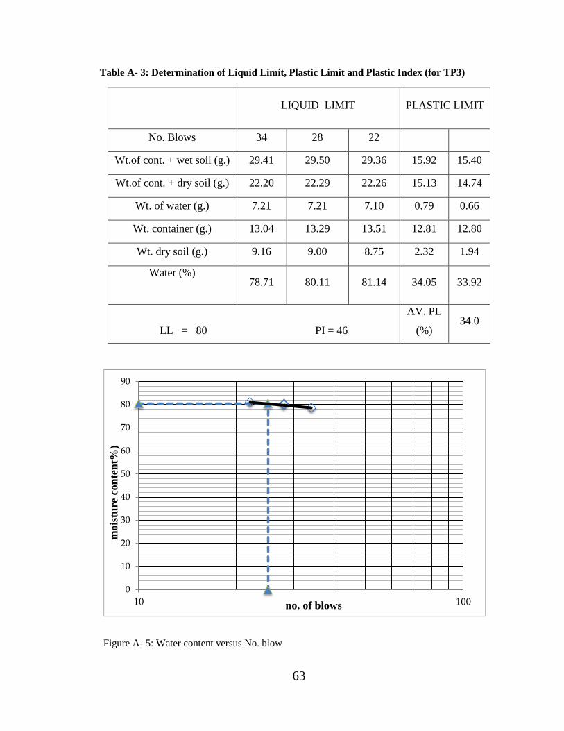
63
Table A- 3: Determination of Liquid Limit, Plastic Limit and Plastic Index (for TP3)
LIQUID LIMIT PLASTIC LIMIT
No. Blows 34 28 22
Wt.of cont. + wet soil (g.) 29.41 29.50 29.36 15.92 15.40
Wt.of cont. + dry soil (g.) 22.20 22.29 22.26 15.13 14.74
Wt. of water (g.) 7.21 7.21 7.10 0.79 0.66
Wt. container (g.) 13.04 13.29 13.51 12.81 12.80
Wt. dry soil (g.) 9.16 9.00 8.75 2.32 1.94
Water (%)
78.71 80.11 81.14 34.05 33.92
LL = 80 PI = 46
AV. PL
(%) 34.0
Figure A- 5: Water content versus No. blow
0
10
20
30
40
50
60
70
80
90
10 100no. of blows
mois
ture
con
ten
t%)
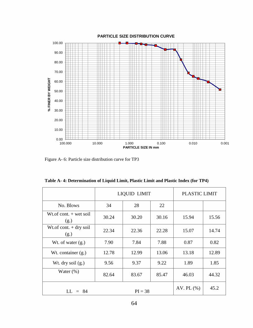
64
Figure A- 6: Particle size distribution curve for TP3
Table A- 4: Determination of Liquid Limit, Plastic Limit and Plastic Index (for TP4)
LIQUID LIMIT PLASTIC LIMIT
No. Blows 34 28 22
Wt.of cont. + wet soil
(g.) 30.24 30.20 30.16 15.94 15.56
Wt.of cont. + dry soil
(g.) 22.34 22.36 22.28 15.07 14.74
Wt. of water (g.) 7.90 7.84 7.88 0.87 0.82
Wt. container (g.) 12.78 12.99 13.06 13.18 12.89
Wt. dry soil (g.) 9.56 9.37 9.22 1.89 1.85
Water (%)
82.64 83.67 85.47 46.03 44.32
LL = 84 PI = 38 AV. PL (%) 45.2
0.00
10.00
20.00
30.00
40.00
50.00
60.00
70.00
80.00
90.00
100.00
0.0010.0100.1001.00010.000100.000
% F
INE
R B
Y W
EIG
HT
PARTICLE SIZE IN mm
PARTICLE SIZE DISTRIBUTION CURVE
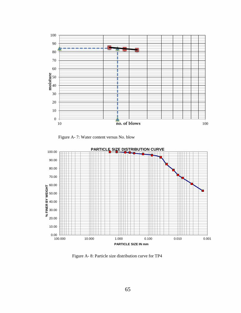
65
Figure A- 7: Water content versus No. blow
Figure A- 8: Particle size distribution curve for TP4
0
10
20
30
40
50
60
70
80
90
100
10 100no. of blows
mo
istu
re
0.00
10.00
20.00
30.00
40.00
50.00
60.00
70.00
80.00
90.00
100.00
0.0010.0100.1001.00010.000100.000
% F
INE
R B
Y W
EIG
HT
PARTICLE SIZE IN mm
PARTICLE SIZE DISTRIBUTION CURVE
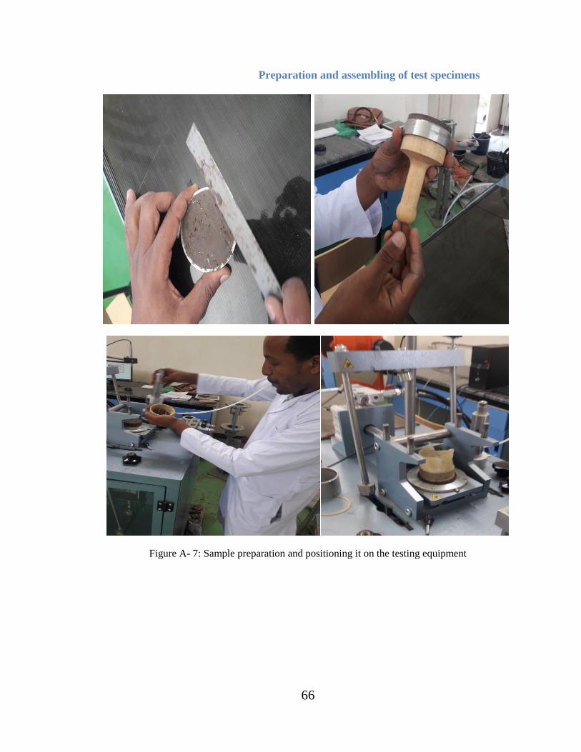
66
Preparation and assembling of test specimens
Figure A- 7: Sample preparation and positioning it on the testing equipment
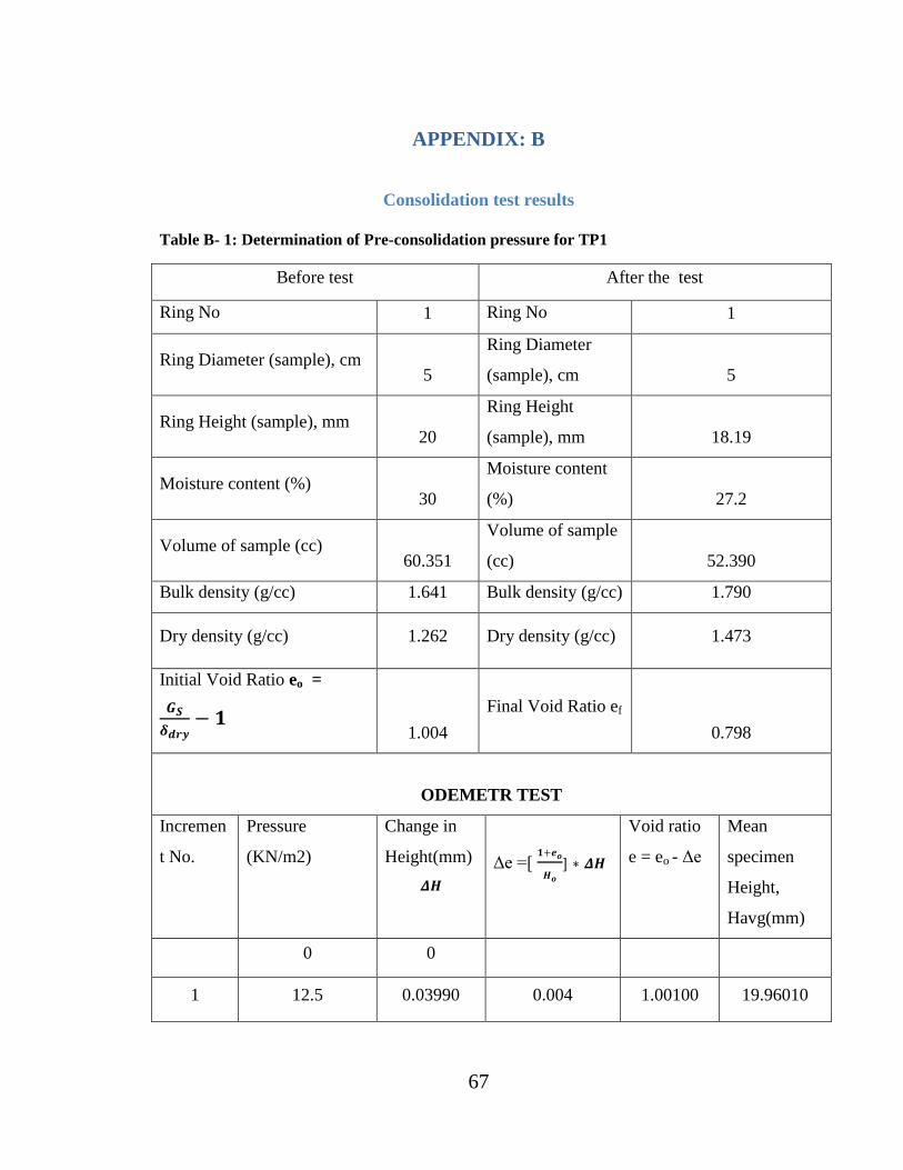
67
APPENDIX: B
Consolidation test results
Table B- 1: Determination of Pre-consolidation pressure for TP1
Before test After the test
Ring No 1 Ring No 1
Ring Diameter (sample), cm 5
Ring Diameter
(sample), cm 5
Ring Height (sample), mm 20
Ring Height
(sample), mm 18.19
Moisture content (%) 30
Moisture content
(%) 27.2
Volume of sample (cc) 60.351
Volume of sample
(cc) 52.390
Bulk density (g/cc) 1.641 Bulk density (g/cc) 1.790
Dry density (g/cc) 1.262 Dry density (g/cc) 1.473
Initial Void Ratio eo =
1.004
Final Void Ratio ef
0.798
ODEMETR TEST
Incremen
t No.
Pressure
(KN/m2)
Change in
Height(mm)
Δe =[
Void ratio
e = eo - Δe
Mean
specimen
Height,
Havg(mm)
0 0
1 12.5 0.03990 0.004 1.00100 19.96010
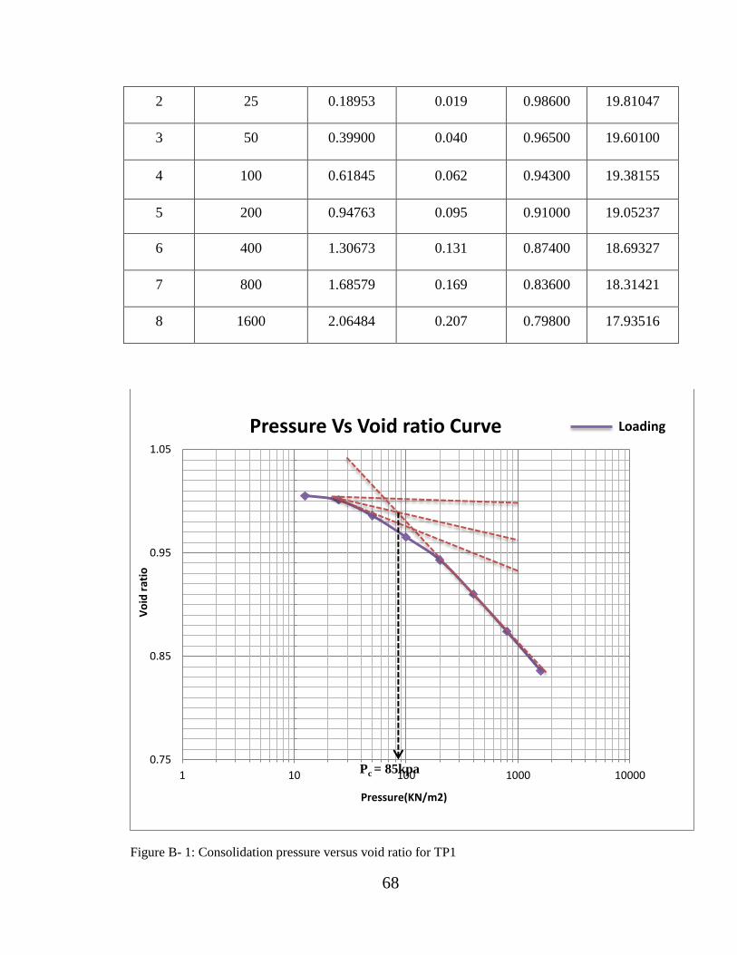
68
2 25 0.18953 0.019 0.98600 19.81047
3 50 0.39900 0.040 0.96500 19.60100
4 100 0.61845 0.062 0.94300 19.38155
5 200 0.94763 0.095 0.91000 19.05237
6 400 1.30673 0.131 0.87400 18.69327
7 800 1.68579 0.169 0.83600 18.31421
8 1600 2.06484 0.207 0.79800 17.93516
Figure B- 1: Consolidation pressure versus void ratio for TP1
0.75
0.85
0.95
1.05
1 10 100 1000 10000
Vo
id r
atio
Pressure(KN/m2)
Pressure Vs Void ratio Curve Loading
Pc = 85kpa
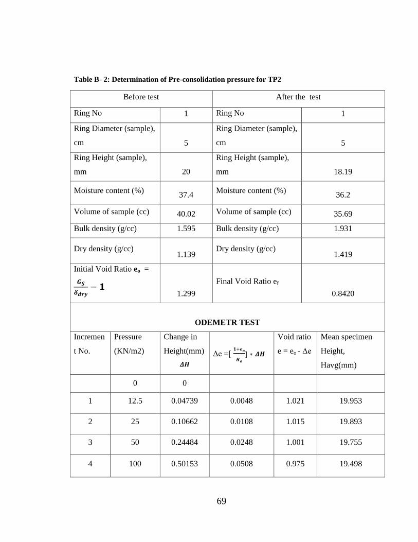
69
Table B- 2: Determination of Pre-consolidation pressure for TP2
Before test After the test
Ring No 1 Ring No 1
Ring Diameter (sample),
cm 5
Ring Diameter (sample),
cm 5
Ring Height (sample),
mm 20
Ring Height (sample),
mm 18.19
Moisture content (%) 37.4
Moisture content (%) 36.2
Volume of sample (cc) 40.02 Volume of sample (cc) 35.69
Bulk density (g/cc) 1.595 Bulk density (g/cc) 1.931
Dry density (g/cc) 1.139
Dry density (g/cc) 1.419
Initial Void Ratio eo =
1.299
Final Void Ratio ef
0.8420
ODEMETR TEST
Incremen
t No.
Pressure
(KN/m2)
Change in
Height(mm)
Δe =[
Void ratio
e = eo - Δe
Mean specimen
Height,
Havg(mm)
0 0
1 12.5 0.04739 0.0048 1.021 19.953
2 25 0.10662 0.0108 1.015 19.893
3 50 0.24484 0.0248 1.001 19.755
4 100 0.50153 0.0508 0.975 19.498
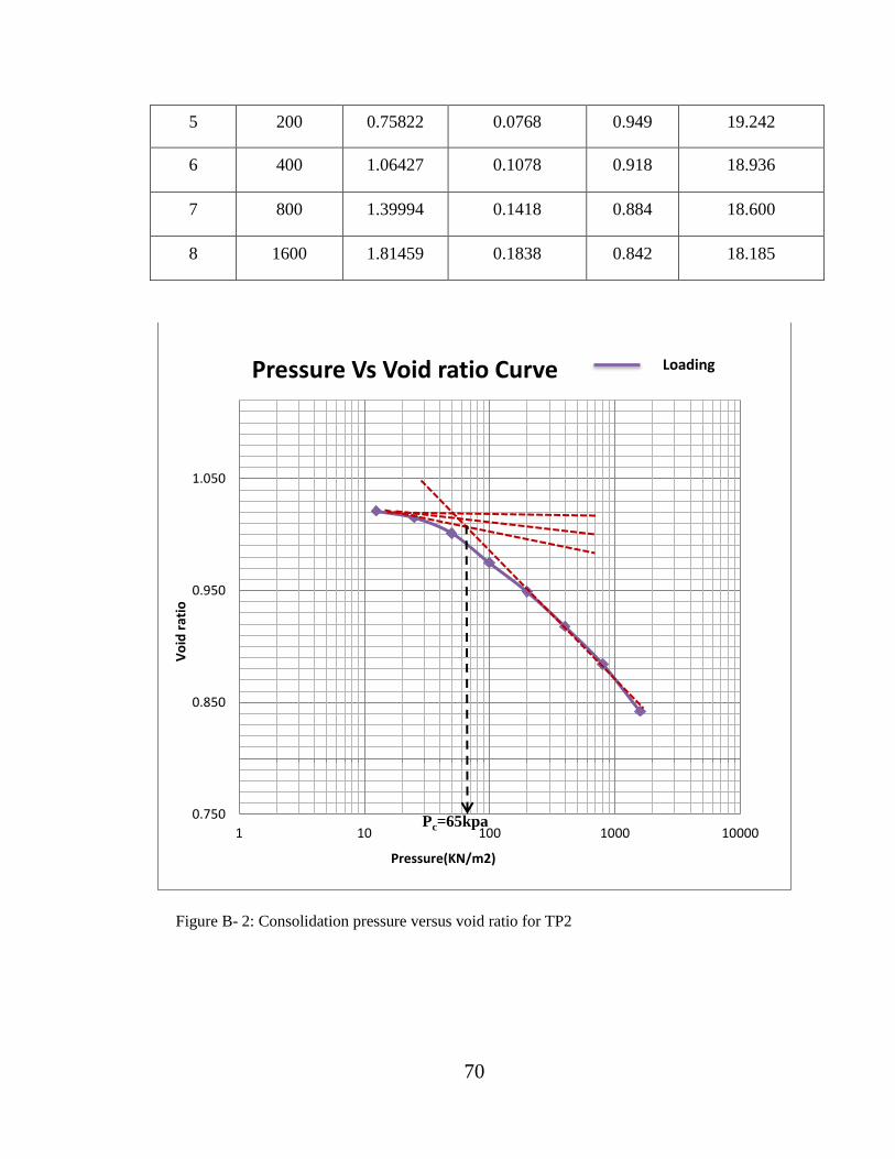
70
5 200 0.75822 0.0768 0.949 19.242
6 400 1.06427 0.1078 0.918 18.936
7 800 1.39994 0.1418 0.884 18.600
8 1600 1.81459 0.1838 0.842 18.185
Figure B- 2: Consolidation pressure versus void ratio for TP2
0.750
0.850
0.950
1.050
1 10 100 1000 10000
Vo
id r
atio
Pressure(KN/m2)
Pressure Vs Void ratio Curve
Pc=65kpa
Loading
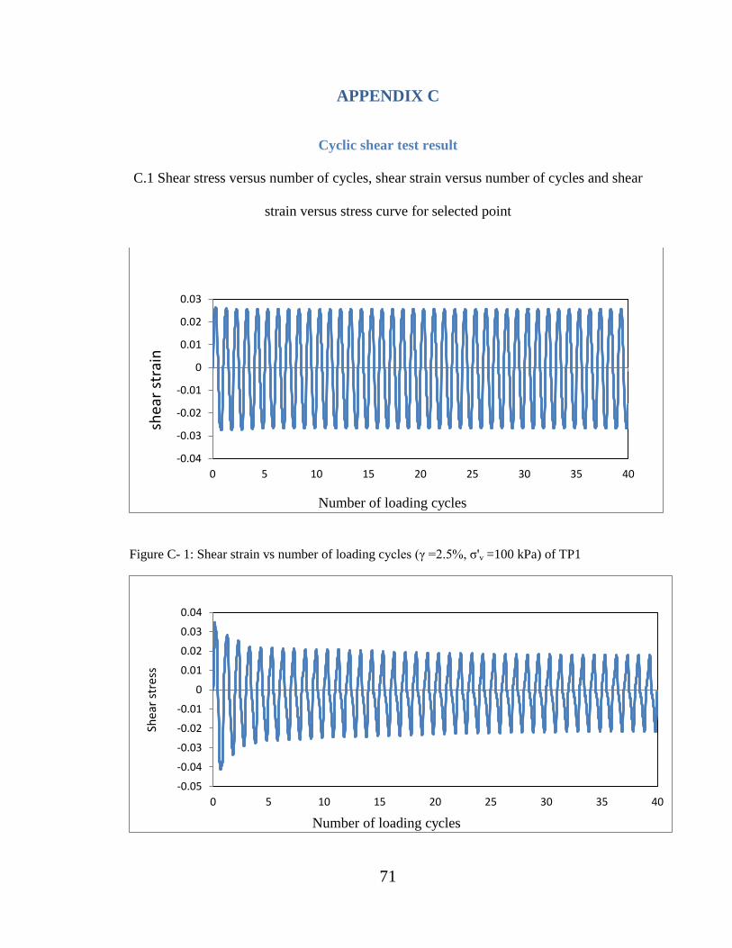
71
APPENDIX C
Cyclic shear test result
C.1 Shear stress versus number of cycles, shear strain versus number of cycles and shear
strain versus stress curve for selected point
Figure C- 1: Shear strain vs number of loading cycles (γ =2.5%, σ'v =100 kPa) of TP1
-0.04
-0.03
-0.02
-0.01
0
0.01
0.02
0.03
0 5 10 15 20 25 30 35 40
Number of loading cycles
shea
r st
rain
-0.05
-0.04
-0.03
-0.02
-0.01
0
0.01
0.02
0.03
0.04
0 5 10 15 20 25 30 35 40
Number of loading cycles
Shea
r st
ress
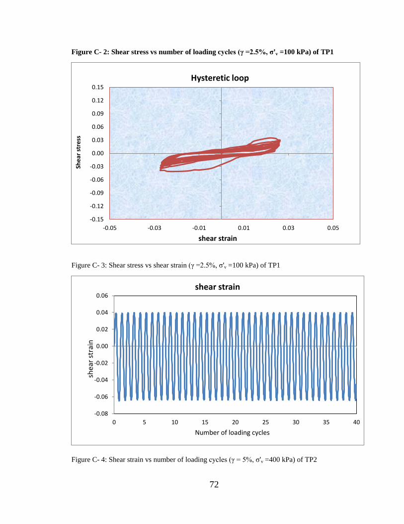
72
Figure C- 2: Shear stress vs number of loading cycles (γ =2.5%, σ'v =100 kPa) of TP1
Figure C- 3: Shear stress vs shear strain (γ =2.5%, σ'v =100 kPa) of TP1
Figure C- 4: Shear strain vs number of loading cycles (γ = 5%, σ'v =400 kPa) of TP2
-0.15
-0.12
-0.09
-0.06
-0.03
0.00
0.03
0.06
0.09
0.12
0.15
-0.05 -0.03 -0.01 0.01 0.03 0.05
She
ar s
tre
ss
shear strain
Hysteretic loop
-0.08
-0.06
-0.04
-0.02
0.00
0.02
0.04
0.06
0 5 10 15 20 25 30 35 40
shear strain
Number of loading cycles
shea
r st
rain
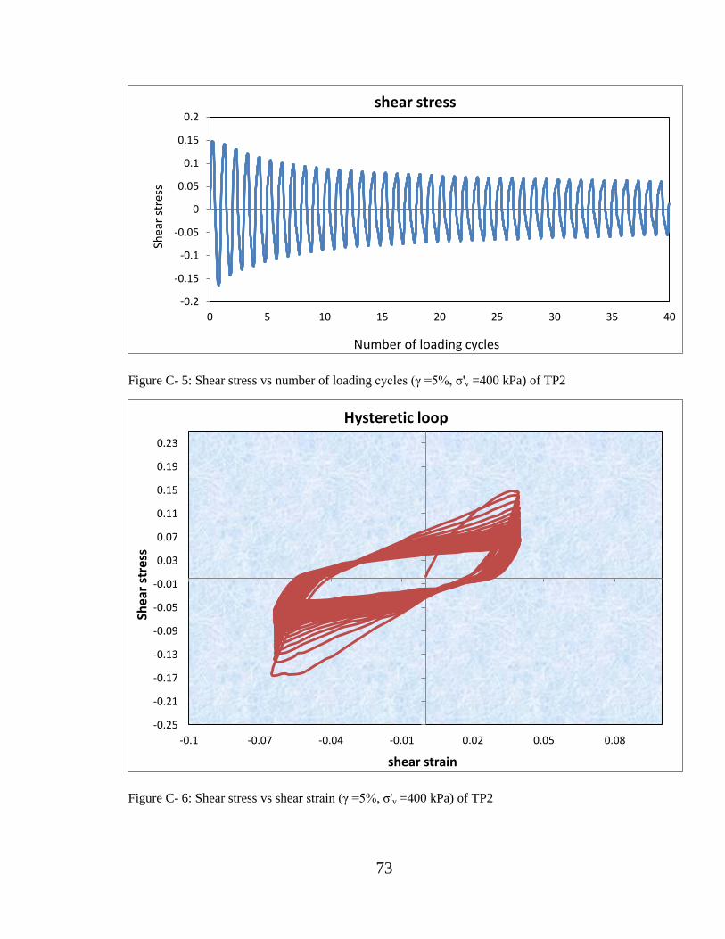
73
Figure C- 5: Shear stress vs number of loading cycles (γ =5%, σ'v =400 kPa) of TP2
Figure C- 6: Shear stress vs shear strain (γ =5%, σ'v =400 kPa) of TP2
-0.2
-0.15
-0.1
-0.05
0
0.05
0.1
0.15
0.2
0 5 10 15 20 25 30 35 40
shear stress
Number of loading cycles
Shea
r st
ress
-0.25
-0.21
-0.17
-0.13
-0.09
-0.05
-0.01
0.03
0.07
0.11
0.15
0.19
0.23
-0.1 -0.07 -0.04 -0.01 0.02 0.05 0.08
Shea
r st
ress
shear strain
Hysteretic loop
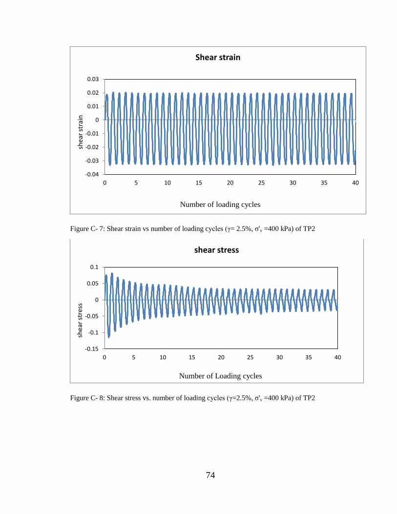
74
Figure C- 7: Shear strain vs number of loading cycles (γ= 2.5%, σ'v =400 kPa) of TP2
Figure C- 8: Shear stress vs. number of loading cycles (γ=2.5%, σ'v =400 kPa) of TP2
-0.04
-0.03
-0.02
-0.01
0
0.01
0.02
0.03
0 5 10 15 20 25 30 35 40
Shear strain
Number of loading cycles
shea
r st
rain
-0.15
-0.1
-0.05
0
0.05
0.1
0 5 10 15 20 25 30 35 40
shear stress
Number of Loading cycles
shea
r st
ress
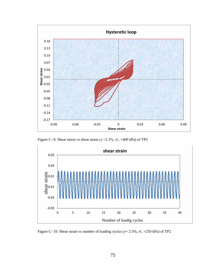
75
Figure C- 9: Shear stress vs shear strain (γ =2.5%, σ'v =400 kPa) of TP2
Figure C- 10: Shear strain vs number of loading cycles (γ= 2.5%, σ'v =250 kPa) of TP2
-0.17
-0.14
-0.11
-0.08
-0.05
-0.02
0.01
0.04
0.07
0.10
0.13
0.16
-0.09 -0.06 -0.03 0 0.03 0.06 0.09
She
ar s
tre
ss
Shear strain
Hysteretic loop
-0.05
-0.03
-0.01
0.01
0.03
0.05
0 5 10 15 20 25 30 35 40
shear strain
Number of loadig cycles
shea
r st
rain
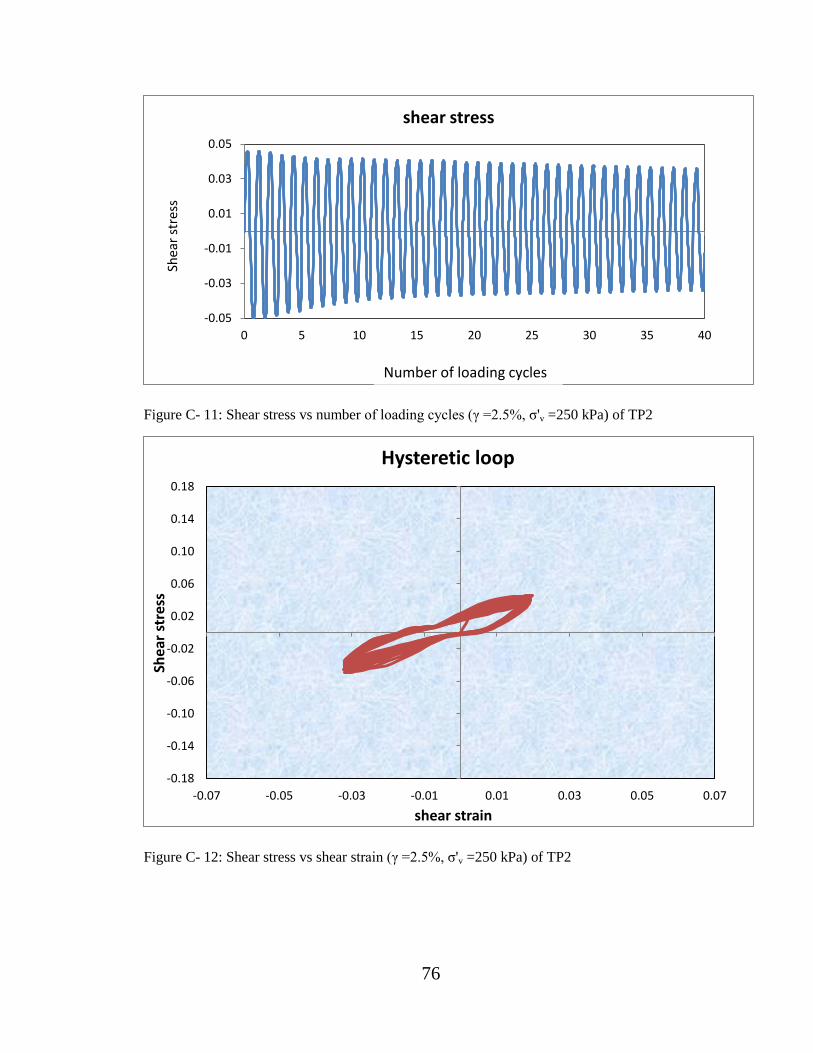
76
Figure C- 11: Shear stress vs number of loading cycles (γ =2.5%, σ'v =250 kPa) of TP2
Figure C- 12: Shear stress vs shear strain (γ =2.5%, σ'v =250 kPa) of TP2
-0.05
-0.03
-0.01
0.01
0.03
0.05
0 5 10 15 20 25 30 35 40
shear stress
Number of loading cycles
Shea
r st
ress
-0.18
-0.14
-0.10
-0.06
-0.02
0.02
0.06
0.10
0.14
0.18
-0.07 -0.05 -0.03 -0.01 0.01 0.03 0.05 0.07
She
ar s
tres
s
shear strain
Hysteretic loop
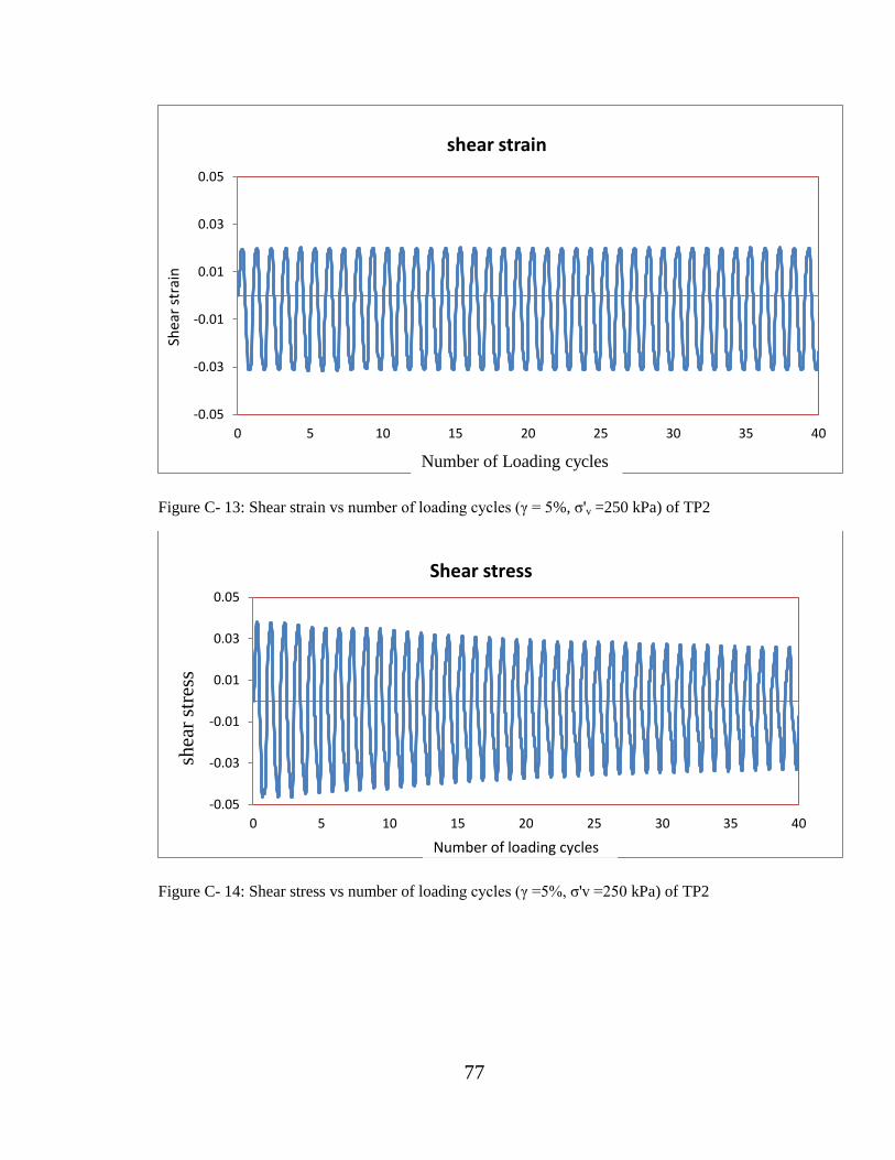
77
Figure C- 13: Shear strain vs number of loading cycles (γ = 5%, σ'v =250 kPa) of TP2
Figure C- 14: Shear stress vs number of loading cycles (γ =5%, σ'v =250 kPa) of TP2
-0.05
-0.03
-0.01
0.01
0.03
0.05
0 5 10 15 20 25 30 35 40
shear strain
Number of Loading cycles
Shea
r st
rain
-0.05
-0.03
-0.01
0.01
0.03
0.05
0 5 10 15 20 25 30 35 40
Shear stress
shea
r st
ress
Number of loading cycles
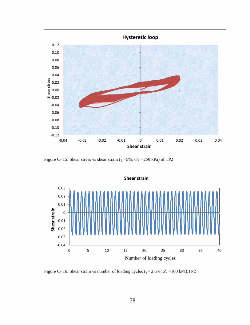
78
Figure C- 15: Shear stress vs shear strain (γ =5%, σ'v =250 kPa) of TP2
Figure C- 16: Shear strain vs number of loading cycles (γ= 2.5%, σ'v =100 kPa),TP2
-0.12
-0.10
-0.08
-0.06
-0.04
-0.02
0.00
0.02
0.04
0.06
0.08
0.10
0.12
-0.04 -0.03 -0.02 -0.01 0 0.01 0.02 0.03 0.04
She
ar s
tre
ss
Shear strain
Hysteretic loop
-0.04
-0.03
-0.02
-0.01
0
0.01
0.02
0.03
0 5 10 15 20 25 30 35 40
Shear strain
Number of loading cycles
Shes
r st
rain
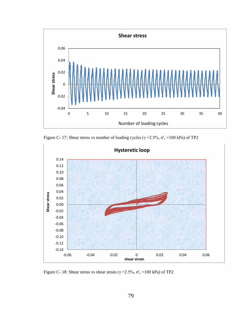
79
Figure C- 17: Shear stress vs number of loading cycles (γ =2.5%, σ'v =100 kPa) of TP2
Figure C- 18: Shear stress vs shear strain (γ =2.5%, σ'v =100 kPa) of TP2
-0.04
-0.02
0
0.02
0.04
0.06
0 5 10 15 20 25 30 35 40
Shear stress
Number of loading cycles
Shea
r st
ress
-0.14
-0.12
-0.10
-0.08
-0.06
-0.04
-0.02
0.00
0.02
0.04
0.06
0.08
0.10
0.12
0.14
-0.06 -0.04 -0.02 0 0.02 0.04 0.06
She
ar s
tre
ss
shear strain
Hysteretic loop
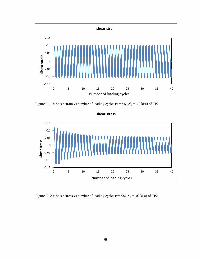
80
Figure C- 19: Shear strain vs number of loading cycles (γ = 5%, σ'v =100 kPa) of TP2
Figure C- 20: Shear stress vs number of loading cycles (γ= 5%, σ'v =100 kPa) of TP2
-0.15
-0.1
-0.05
0
0.05
0.1
0.15
0 5 10 15 20 25 30 35 40
shear strain
Number of loading cycles
Shes
r st
rain
-0.15
-0.1
-0.05
0
0.05
0.1
0.15
0 5 10 15 20 25 30 35 40
shear stress
She
ar s
tre
ss
Number of loading cycles
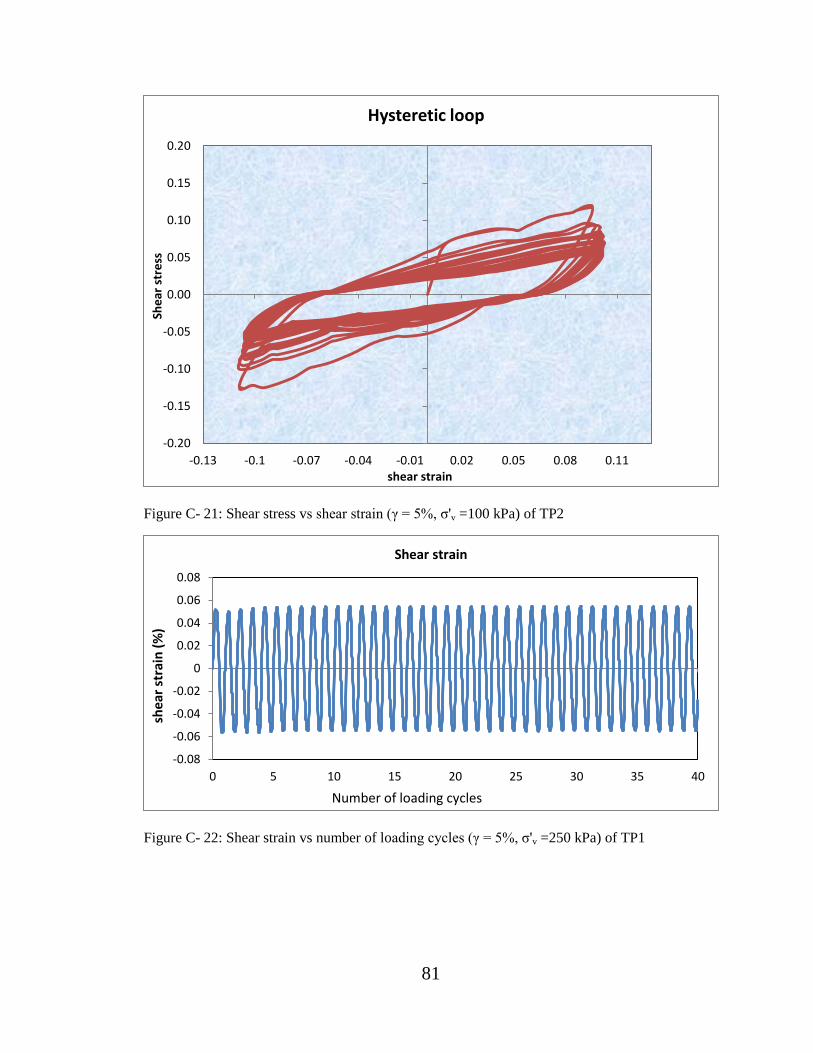
81
Figure C- 21: Shear stress vs shear strain (γ = 5%, σ'v =100 kPa) of TP2
Figure C- 22: Shear strain vs number of loading cycles (γ = 5%, σ'v =250 kPa) of TP1
-0.20
-0.15
-0.10
-0.05
0.00
0.05
0.10
0.15
0.20
-0.13 -0.1 -0.07 -0.04 -0.01 0.02 0.05 0.08 0.11
She
ar s
tre
ss
shear strain
Hysteretic loop
-0.08
-0.06
-0.04
-0.02
0
0.02
0.04
0.06
0.08
0 5 10 15 20 25 30 35 40
Shear strain
shea
r st
rain
(%
)
Number of loading cycles
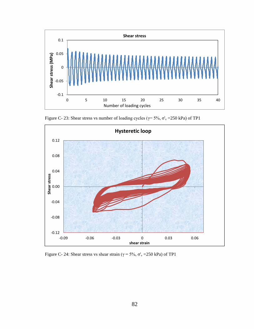
82
Figure C- 23: Shear stress vs number of loading cycles (γ= 5%, σ'v =250 kPa) of TP1
Figure C- 24: Shear stress vs shear strain (γ = 5%, σ'v =250 kPa) of TP1
-0.1
-0.05
0
0.05
0.1
0 5 10 15 20 25 30 35 40
Shear stress
Shea
r st
ress
(M
Pa)
Number of loading cycles
-0.12
-0.08
-0.04
0.00
0.04
0.08
0.12
-0.09 -0.06 -0.03 0 0.03 0.06
She
ar s
tre
ss
shear strain
Hysteretic loop
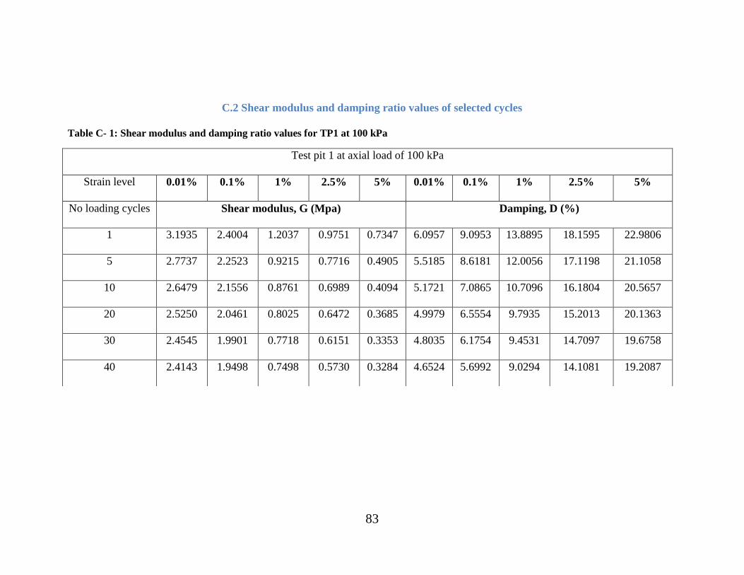
83
C.2 Shear modulus and damping ratio values of selected cycles
Table C- 1: Shear modulus and damping ratio values for TP1 at 100 kPa
Test pit 1 at axial load of 100 kPa
Strain level 0.01% 0.1% 1% 2.5% 5% 0.01% 0.1% 1% 2.5% 5%
No loading cycles Shear modulus, G (Mpa) Damping, D (%)
1 3.1935 2.4004 1.2037 0.9751 0.7347 6.0957 9.0953 13.8895 18.1595 22.9806
5 2.7737 2.2523 0.9215 0.7716 0.4905 5.5185 8.6181 12.0056 17.1198 21.1058
10 2.6479 2.1556 0.8761 0.6989 0.4094 5.1721 7.0865 10.7096 16.1804 20.5657
20 2.5250 2.0461 0.8025 0.6472 0.3685 4.9979 6.5554 9.7935 15.2013 20.1363
30 2.4545 1.9901 0.7718 0.6151 0.3353 4.8035 6.1754 9.4531 14.7097 19.6758
40 2.4143 1.9498 0.7498 0.5730 0.3284 4.6524 5.6992 9.0294 14.1081 19.2087
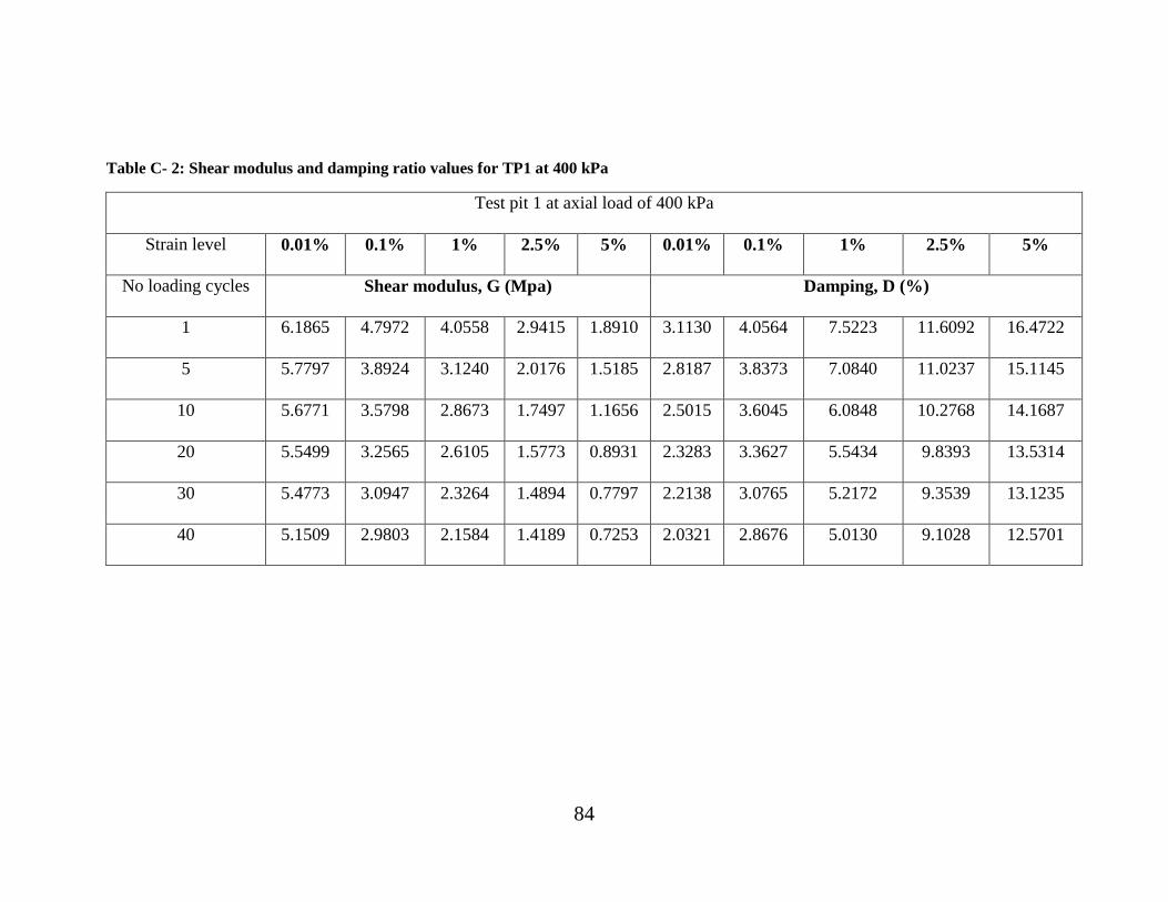
84
Table C- 2: Shear modulus and damping ratio values for TP1 at 400 kPa
Test pit 1 at axial load of 400 kPa
Strain level 0.01% 0.1% 1% 2.5% 5% 0.01% 0.1% 1% 2.5% 5%
No loading cycles Shear modulus, G (Mpa) Damping, D (%)
1 6.1865 4.7972 4.0558 2.9415 1.8910 3.1130 4.0564 7.5223 11.6092 16.4722
5 5.7797 3.8924 3.1240 2.0176 1.5185 2.8187 3.8373 7.0840 11.0237 15.1145
10 5.6771 3.5798 2.8673 1.7497 1.1656 2.5015 3.6045 6.0848 10.2768 14.1687
20 5.5499 3.2565 2.6105 1.5773 0.8931 2.3283 3.3627 5.5434 9.8393 13.5314
30 5.4773 3.0947 2.3264 1.4894 0.7797 2.2138 3.0765 5.2172 9.3539 13.1235
40 5.1509 2.9803 2.1584 1.4189 0.7253 2.0321 2.8676 5.0130 9.1028 12.5701
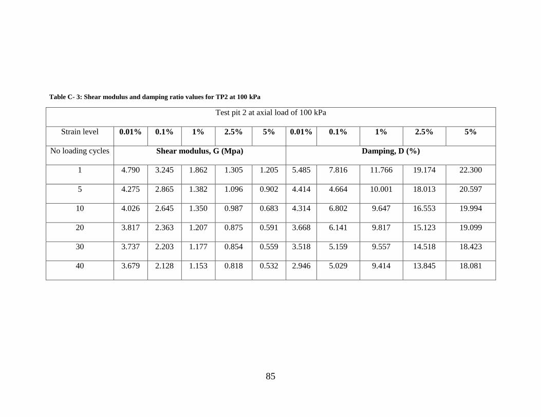
85
Table C- 3: Shear modulus and damping ratio values for TP2 at 100 kPa
Test pit 2 at axial load of 100 kPa
Strain level 0.01% 0.1% 1% 2.5% 5% 0.01% 0.1% 1% 2.5% 5%
No loading cycles Shear modulus, G (Mpa) Damping, D (%)
1 4.790 3.245 1.862 1.305 1.205 5.485 7.816 11.766 19.174 22.300
5 4.275 2.865 1.382 1.096 0.902 4.414 4.664 10.001 18.013 20.597
10 4.026 2.645 1.350 0.987 0.683 4.314 6.802 9.647 16.553 19.994
20 3.817 2.363 1.207 0.875 0.591 3.668 6.141 9.817 15.123 19.099
30 3.737 2.203 1.177 0.854 0.559 3.518 5.159 9.557 14.518 18.423
40 3.679 2.128 1.153 0.818 0.532 2.946 5.029 9.414 13.845 18.081

86
Table C- 4: Shear modulus and damping ratio values for TP2 at 250 kPa
Test pit 2 at axial load of 250 kPa
Strain level 0.01% 0.1% 1% 2.5% 5% 0.01% 0.1% 1% 2.5% 5%
No loading cycles Shear modulus, G (Mpa) Damping, D (%)
1 5.2940 3.4649 2.3098 1.8640 1.6635 4.3963 5.6546 11.3040 17.9907 21.4053
5 4.6214 3.0863 1.9943 1.7625 1.5470 4.0011 5.5740 10.1120 15.1611 20.6587
10 4.2547 2.9595 1.8773 1.6125 1.5148 3.9693 5.0766 9.4392 14.0312 18.6124
20 4.0404 2.7154 1.7511 1.5003 1.3116 3.5799 4.8949 8.9707 12.7278 17.4257
30 3.9222 2.6577 1.6466 1.4364 1.2158 3.2283 4.7205 8.4797 12.9924 16.1994
40 3.8057 2.5902 1.5853 1.3837 1.1521 2.8293 4.6188 8.0618 12.4454 15.8514
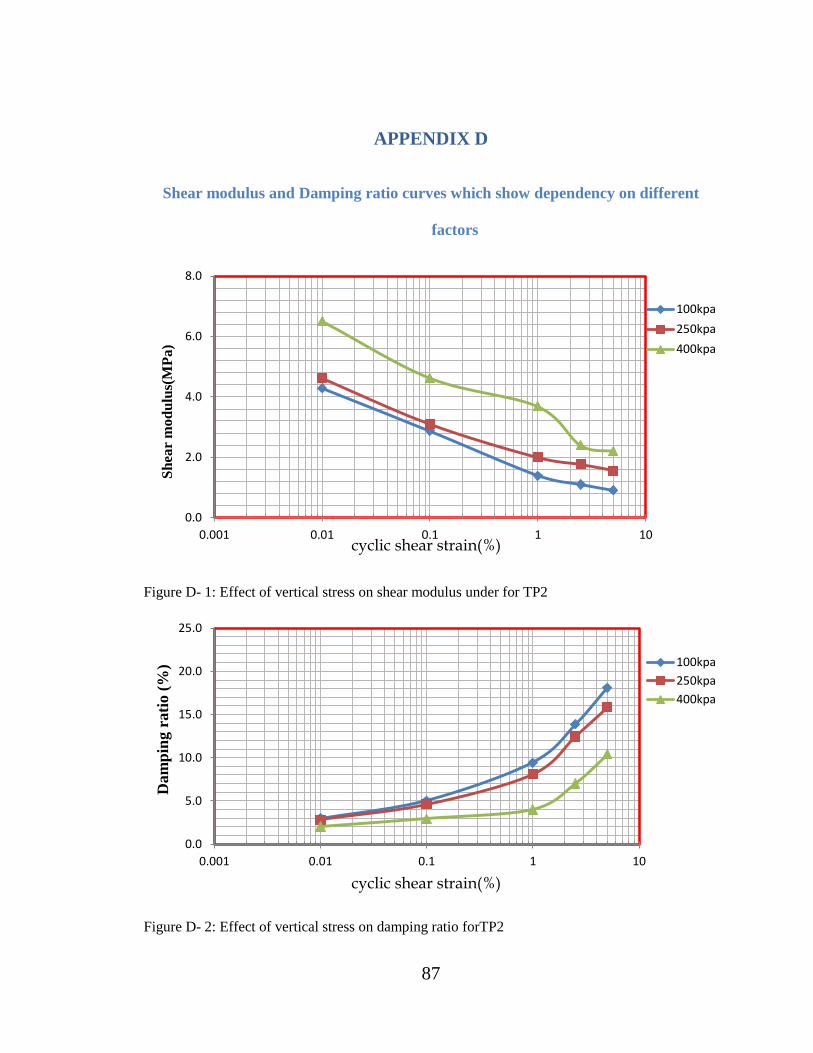
87
APPENDIX D
Shear modulus and Damping ratio curves which show dependency on different
factors
Figure D- 1: Effect of vertical stress on shear modulus under for TP2
Figure D- 2: Effect of vertical stress on damping ratio forTP2
0.0
2.0
4.0
6.0
8.0
0.001 0.01 0.1 1 10
100kpa
250kpa
400kpa
cyclic shear strain(%)
Sh
ear
mo
du
lus(
MP
a)
0.0
5.0
10.0
15.0
20.0
25.0
0.001 0.01 0.1 1 10
100kpa
250kpa
400kpa
cyclic shear strain(%)
Dam
pin
g r
ati
o (
%)
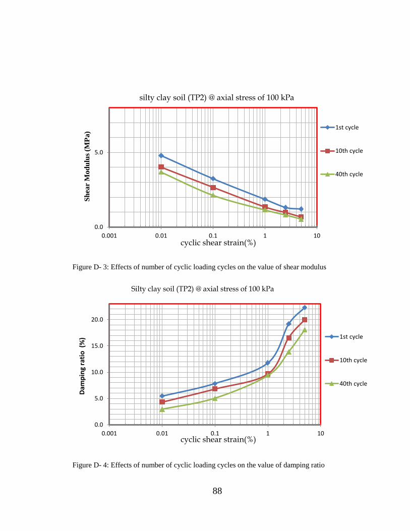
88
Figure D- 3: Effects of number of cyclic loading cycles on the value of shear modulus
Figure D- 4: Effects of number of cyclic loading cycles on the value of damping ratio
0.0
5.0
0.001 0.01 0.1 1 10
1st cycle
10th cycle
40th cycle
cyclic shear strain(%)
silty clay soil (TP2) @ axial stress of 100 kPa
Sh
ear
Mo
du
lus
(MP
a)
0.0
5.0
10.0
15.0
20.0
0.001 0.01 0.1 1 10
1st cycle
10th cycle
40th cycle
cyclic shear strain(%)
Silty clay soil (TP2) @ axial stress of 100 kPa
Dam
pin
g ra
tio
(%
)
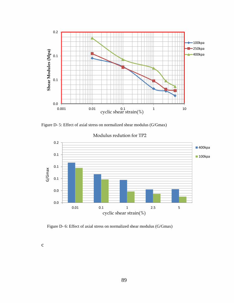
89
Figure D- 5: Effect of axial stress on normalized shear modulus (G/Gmax)
Figure D- 6: Effect of axial stress on normalized shear modulus (G/Gmax)
c
0.0
0.1
0.1
0.2
0.001 0.01 0.1 1 10
100kpa
250kpa
400kpa
cyclic shear strain(%)
Sh
ea
r M
od
ule
s (M
pa
)
0.0
0.0
0.1
0.1
0.1
0.2
0.01 0.1 1 2.5 5
400kpa
100kpa
cyclic shear strain(%)
G/G
max
Modulus redution for TP2