CYCLONE GLOBAL NAVIGATION SATELLITE SYSTEM (CYGNSS)

Algorithm Theoretical Basis Document

Level 1A DDM Calibration

UM Doc. No. 148-0136-X1SwRI Doc. No. N/ARevision 1Date 19 December 2014Contract NNL13AQ00C

Algorithm Theoretical Basis Documents (ATBDs) provide the physical and mathematical descriptions of the algorithms used in the generation of science data products. The ATBDs include a description of variance and uncertainty estimates and considerations of calibration and validation, exception control and diagnostics. Internal and external data flows are also described.

CYCLONE GLOBAL NAVIGATION SATELLITE SYSTEM (CYGNSS)

Algorithm Theoretical Basis Document

Level 1A DDM Calibration

UM Doc. No. 148-0136-X1SwRI Doc. No. N/ARevision 1Date 19 Dec 2014Contract NNL13AQ00C

Prepared by: Date: Scott Gleason, Southwest Research Institute

Approved by: Date: Chris Ruf, CYGNSS Principal Investigator Approved by: Date: John Scherrer, CYGNSS Project Manager Approved by: Date: Randy Rose, CYGNSS Project Systems Engineer Released by: Date: Damen Provost, CYGNSS UM Project Manager

ATBD Level 1A DDM Calibration UM: 148-0136-X1 SwRI: N/A Rev 1 Chg 0 Page iii

REVISION NOTICE

Document Revision History

Revision Date Changes

PRE-RELEASE DRAFT 17 June 2013 n/a

INITIAL RELEASE 14 January 2014 Add explicit algorithms for use of internal black body target and estimation of receiver noise temperature. Add detailed error analysis.

Rev 1 19 December 2014 Same basic approach but greater detail and examples provided of algorithm implementation.

XXX 1

CYGNSS Level 1a DDM Calibration and ErrorAnalysis

This is a portion of the overall Level 1 Calibration Algorithm Theoretical Basis Document (ATBD) describing the Level 1acalibration and error analysis.

I. LEVEL 1A CALIBRATION ALGORITHM: COUNTS TO WATTS

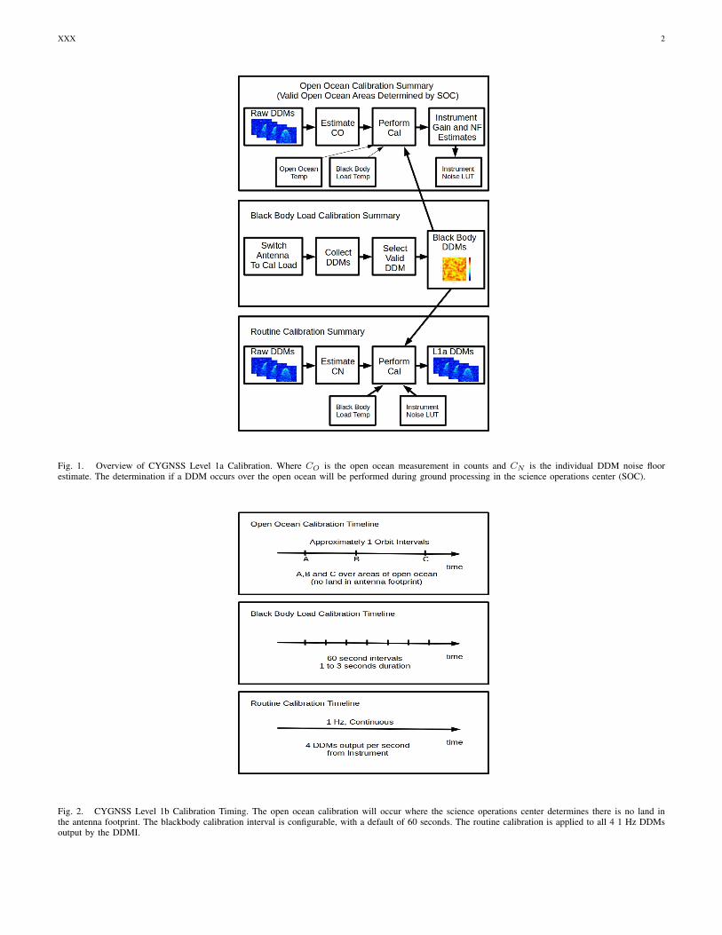
Individual bins of the DDM generated by the Delay Doppler Mapping Instrument (DDMI) are measured in raw, uncalibratedunits referred to as ”counts”. These counts are linearly related to the total signal power processed by the DDMI. In addition tothe ocean surface scattered Global Positioning System (GPS) signal, the total signal includes contributions from the thermalemission by the Earth and by the DDMI itself. The power in the total signal is the product of all the input signals, multipliedby the gain of the DDMI receiver. Level 1a calibration converts each bin in the DDM from raw counts to units of watts. Aflowchart of the L1a calibration procedure is shown in Figure 1.

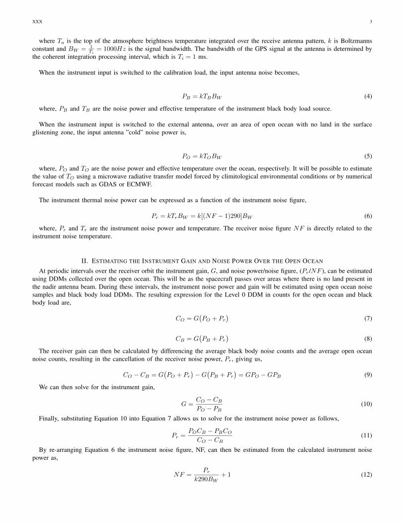
1) Calibration Intervals: The open ocean calibration will occur approximately every orbit and the black body calibrationwill be performed every 60 seconds on-orbit for each nadir science antenna. The routine calibration will be performed at1Hz on all DDM’s output by the DDMI (4 per second). Figure 2 illustrates the actions performed and intervals for all of theCYGNSS L1a calibration steps.

A. Raw Level 0 Delay Doppler Map

The DDM values output from the CYGNSS science instrument will be sent to the CYGNSS spacecraft as arbitrary counts.The count values will be a result of the signal travelling through the various stages of the instrument, which will add a gain tothe received power levels. The value of the DDM in arbitrary counts can be linked to the arriving signal power in Watts such that,

C = G(Pa + Pr + Pg

)(1)

where,C are the DDM values in counts output from the instrument at each delay/Doppler bin.Pa is the thermal noise power generated by the antenna in watts.Pr is the thermal noise power generated by the instrument in watts.Pg is the scattered signal power at the instrument in watts.G is the total instrument gain applied to the incoming signal in counts per watt.

The terms, C and Pg are functions of delay and Doppler while Pa and Pr are assumed to be independent of the delayDoppler bin in the DDM. Every DDM includes a number of delay bins where signal power is not present and an individualDDM noise floor level can be estimated. These bins physically represents delays above the ocean surface. These delay andDoppler bins provide an estimate of the DDM noise power, expressed in counts as,

CN = G(Pa + Pr

)(2)

Assuming Pa and Pr are independent of delay and Doppler, the DDM samples above the ocean surface can be used toestimate the noise only contribution to the raw counts.

B. Noise Power Expressions

The input antenna noise can be generically expressed as,

Pa = kTaBW (3)

XXX 2

Fig. 1. Overview of CYGNSS Level 1a Calibration. Where CO is the open ocean measurement in counts and CN is the individual DDM noise floorestimate. The determination if a DDM occurs over the open ocean will be performed during ground processing in the science operations center (SOC).

Fig. 2. CYGNSS Level 1b Calibration Timing. The open ocean calibration will occur where the science operations center determines there is no land inthe antenna footprint. The blackbody calibration interval is configurable, with a default of 60 seconds. The routine calibration is applied to all 4 1 Hz DDMsoutput by the DDMI.

XXX 3

where Ta is the top of the atmosphere brightness temperature integrated over the receive antenna pattern, k is Boltzmannsconstant and BW = 1

Ti= 1000Hz is the signal bandwidth. The bandwidth of the GPS signal at the antenna is determined by

the coherent integration processing interval, which is Ti = 1 ms.

When the instrument input is switched to the calibration load, the input antenna noise becomes,

PB = kTBBW (4)

where, PB and TB are the noise power and effective temperature of the instrument black body load source.

When the instrument input is switched to the external antenna, over an area of open ocean with no land in the surfaceglistening zone, the input antenna ”cold” noise power is,

PO = kTOBW (5)

where, PO and TO are the noise power and effective temperature over the ocean, respectively. It will be possible to estimatethe value of TO using a microwave radiative transfer model forced by climitological environmental conditions or by numericalforecast models such as GDAS or ECMWF.

The instrument thermal noise power can be expressed as a function of the instrument noise figure,

Pr = kTrBW = k[(NF − 1)290]BW (6)

where, Pr and Tr are the instrument noise power and temperature. The receiver noise figure NF is directly related to theinstrument noise temperature.

II. ESTIMATING THE INSTRUMENT GAIN AND NOISE POWER OVER THE OPEN OCEAN

At periodic intervals over the receiver orbit the instrument gain, G, and noise power/noise figure, (Pr/NF ), can be estimatedusing DDMs collected over the open ocean. This will be as the spacecraft passes over areas where there is no land present inthe nadir antenna beam. During these intervals, the instrument noise power and gain will be estimated using open ocean noisesamples and black body load DDMs. The resulting expression for the Level 0 DDM in counts for the open ocean and blackbody load are,

CO = G(PO + Pr

)(7)

CB = G(PB + Pr

)(8)

The receiver gain can then be calculated by differencing the average black body noise counts and the average open oceannoise counts, resulting in the cancellation of the receiver noise power, Pr, giving us,

CO − CB = G(PO + Pr

)−G

(PB + Pr

)= GPO −GPB (9)

We can then solve for the instrument gain,

G =CO − CB

PO − PB(10)

Finally, substituting Equation 10 into Equation 7 allows us to solve for the instrument noise power as follows,

Pr =POCB − PBCO

CO − CB(11)

By re-arranging Equation 6 the instrument noise figure, NF, can then be estimated from the calculated instrument noisepower as,

NF =Pr

k290BW+ 1 (12)

XXX 4

III. ROUTINE CALIBRATION OF SIGNAL POWER

The generic instrument DDM in counts is expressed in Equation 1, which includes the received signal power, Pg . TheseDDMs will be generated by the instrument every second and will be corrected by the estimated noise floor using Equation 2,such that we are left with a signal only DDM,

Cg = C − CN = GPg (13)

Subsequently the instrument gain at the collection time of this DDM can be calculated using the current estimate of the blackbody load noise temperature, TB , and the last (corrected) open ocean calibration estimate of the instrument noise power, Pr.This is achieved by re-arranging Equation 13 into an expression of the instrument gain, and setting this equal to the instrumentgain estimated directly from the black body load DDM calculated from Equation 8,

G =C − CN

Pg=

CB

PB + Pr(14)

where, CB is the mean count value of the last black body load DDM.PB is the estimated black body load noise power estimated using the last thermistor temperature reading near the load itselfin the LNA, and Equation 4.Pr is the last estimate of the instrument noise power, estimated from a noise figure vs temperature look up table and validatedduring the open ocean calibration sequence.

A. Generating the Level 1a Data Product

The routine calibration assumes that the Gain, G, antenna noise temperature, Ta and the instrument noise power, Pr remainconstant over the combined collection interval for Equation 1 (DDM to be calibrated), Equation 2 (Noise floor estimate forthe DDM being calibrated) and Equation 8 (the black body load noise DDM). By substituting Equation 14 into Equation 13and solving for the signal power term, Pg we arrive at the final Level 1a calibration,

Pg =(C − CN )(PB + Pr)

CB(15)

B. Consideration of Time and Temperature Dependencies

All of the terms in Equation 15 are collected at slightly different times than the actual science measurements themselves,and during these time intervals it is possible that the noise temperatures can vary slightly from the measurement time. Eachof the terms in the Level 1a calibration equation is addressed below with regard to this time difference,

1) C. The science measurement is made once per second and provides the reference time for all of the other parameters.2) CN The noise measurements for each science DDM are made at delays above the ocean surface, which are only on the

order of a handful of microseconds from the time of the science measurement.3) PB the blackbody target power is determined from a physical temperature sensor measured at 1 Hz and near enough in

time to the 1 Hz science measurements that the physical temperature will not have changed significantly between thethermistor reading and the science measurement.

4) Pr the receiver noise power is derived from open ocean measurements that may have been made minutes or hours apartfrom the science measurement. During this time it is possible that the instrument noise temperature will have changed.How this is mitigated is described below.

5) CB the blackbody target measurement is made within 30 seconds of the science measurement, and close enough in timethat the receiver gain noise figure have not changed significantly.

One term in Equation 15, the receiver noise power, Pr, is derived from measurements that may have been made minutesor possibly hours apart from the science measurements. As such, it is possible that Pr has changed in that time. In order toaddress this, a temperature dependent lookup table will be used to correct Pr. The lookup table will be indexed by the readingsof the same physical temperature sensor used to track the blackbody target temperature. The dependence of Pr on temperaturewill initially be characterized in pre-launch environmental testing and the first flight lookup table will be derived from thosetest data. Once on orbit, open ocean measurements will be used to validate Pr using Equation 11. As open ocean data areassembled over a range of physical temperatures, the lookup table will be validated and, if necessary updated on orbit.

XXX 5

Flag Derived From Threshold CommentNegative signal power in DDMA area Output of L1a Calibration algorithm 0 Watts C − CN ¡ 0

S/C S-Band transmitter on S/C Housekeeping Telemetry on/off Possible power leakage into L1a DDM noise levelTime since last OO calibration DDMI Operation Sequence TBD Possible larger then normal error in Pr estimate

LNA temperature change since last BB calibration LNA thermistor TBD Possible larger than expected error in PB estimateLand present in DDM ground based land mask TBD Can cause errors in retrievals

Potentially high cross correlation power present number of PRNs in view TBD Can bias noise floor estimateLow confidence in noise floor estimate number of noise samples TBD TBD

Low confidence in OO noise temperature ground based model TBD ???Large step change in noise floor observed Noise floor trend TBD Possible internal or external RFI present

TABLE IL1A QUALITY CONTROL FLAGS SUMMARY.

C. Quality Control Flags

The Level 1a data product will include a set of quality control flags designed to indicate to users potential problems withthe data. These flags, the parameters they are derived from and the default threshold values are listed in Table I. Each of thequality control flags is briefly described below.

1) Negative signal power in DDMA. The DDM Area (DDMA) is used for Level 2 wind speed retrievals and consists of 3delay bins and 5 Doppler bins. This flag will be set if the L1a calibration resulted in any of these bins having negativepower values.

2) S-Band transmitter on. During S/C down link operations, there is a possibility of power leaking into the nadir antennasand biasing the noise floor estimation. This flag will be set for individual DDMs whenever the S-band transmitter wason while the DDM was taken.

3) Time since last open ocean calibration. The open ocean calibration will be performed as the satellite passes over pre-determined regions of land-free ocean. As the intervals between these calibrations will not be regular, the time since thelast calibration will be included for each DDM to flag potentially long gaps between open ocean calibrations.

4) LNA temperature change since last black body load calibration. The black body load calibration will be performed every60 seconds. This flag will indicate a larger than expected temperature change in the LNA since the last black bodycalibration.

5) Land present in DDM. The presence of land in the DDM glistening zone will be flagged so users can potentially filterout land reflections pixels during higher level processing.

6) Low confidence in DDM noise floor estimate. If the estimate of the noise floor for each DDM, CN , is suspected to besignificantly in error this flag will be set.

7) Low confidence in open ocean noise temperature. If the modelled value of the open ocean noise temperature is suspectedto have larger than normal errors this flag will be set.

8) Step change in noise floor observed. The DDM noise floor should change slowly as a function of time. If an abruptchange in the DDM noise floor trend is observed this is an indication that an internal (to the instrument or S/C) orexternal RFI noise source is biasing the DDM noise floor estimate.

IV. ERROR ANALYSIS OF THE LEVEL 1A CALIBRATION ALGORITHM

The Level 1a data product consists of observed signal power, Pg (in Watts) over a range of delay steps and Dopplerfrequencies. This error analysis concentrates on the uncertainties present in the CYGNSS Level 1a calibration algorithm. Eachuncertainty in the Level 1a calibration algorithm will be considered an independent uncorrelated error source. The method forthis error analysis is based on that presented in Jansen et. al [1] for a microwave radiometer. The errors in the L1a calibrationcan be broken into two parts; the estimation of the instrument noise performed during the open ocean calibration sequence,Pr and the routine second by second calibration of the science DDM, Pg .

A. Error Analysis in Open Ocean Instrument Noise Calibration

Equation 11 for the calculation of the instrument noise power is repeated below,

Pr =PBCO − POCB

CB − CO(16)

The total error in the estimate of the instrument noise power, Pr, is the root sum square (RSS) of the individual errorscontributed by the independent terms of Equation 16, expressed as,

XXX 6

∆Pr =

[4∑

i=1

E2(qi)

]1/2(17)

where the partial derivatives of the individual errors terms can be expressed as,

E(qi) =

∣∣∣∣∣∂Pr

∂qi

∣∣∣∣∣∆qi (18)

The individual error quantities are defined as: q1 = PB , q2 = PO, q3 = CB and q4 = CO. The 1-sigma uncertainties inthese quantities are expressed as ∆qi. Using Equation 16 and Equation 18 to evaluate the partial derivative error terms weobtain,

E(PB) =CO

CB − CO∆PB (19)

E(PO) =CB

CB − CO∆PO (20)

E(CB) =POCO − 2POCB + PBCO

(CB − CO)2∆CB (21)

E(CO) =PBCB − 2PBCO + POCB

(CB − CO)2∆CO (22)

The error magnitudes for each of these terms can be approximated as follows:

The black body load, PB , and open ocean PO power can be broken down to their respective temperatures such that,

PB = kTBBW (23)

PO = kTOBW (24)

Resulting in the following expressions for changes in noise power due to uncertainties in the black body and open oceanreference temperatures,

∆PB = k∆TBBW (25)

∆PO = k∆TOBW (26)

where ∆TB and ∆TO are the black body load and open ocean temperature 1-sigma errors.The 1-sigma errors in the observed noise powers, ∆CO and ∆CB , vary as a function of the number of noise samples

collected to estimate the average power level as,

∆CB = std(~CN1

B ) (27)

∆CO = std(~CN1

O ) (28)

Where ~CN1

B and ~CN1

O are noise samples vectors of length N1. Given 20 noise samples in every DDM Doppler row, a fullDDM coresponds to 2560 noise samples.

Quantitative values for each or the error components listed above and the RSS total for open ocean calibration using 2 fullDDMs and instrument noise power estimates using a LUT only are shown in Table II.

XXX 7

Error Term LUT Based N1 = 5120 (2 DDMs) CommentE(PB) N/A 0.05 Black body load power error ∆TB = 2 degE(PO) N/A 0.07 Open ocean power error ∆TB = 2 degE(CB) N/A 0.18 Black body noise floor estimate, countsE(CO) N/A 0.10 Open ocean noise floor estimate, counts

Total RSS Error (∆Pr ) 0.084 0.23 LUT errors and Equation 17

TABLE IIOPEN OCEAN, INSTRUMENT NOISE CALIBRATION ERRORS (DB).

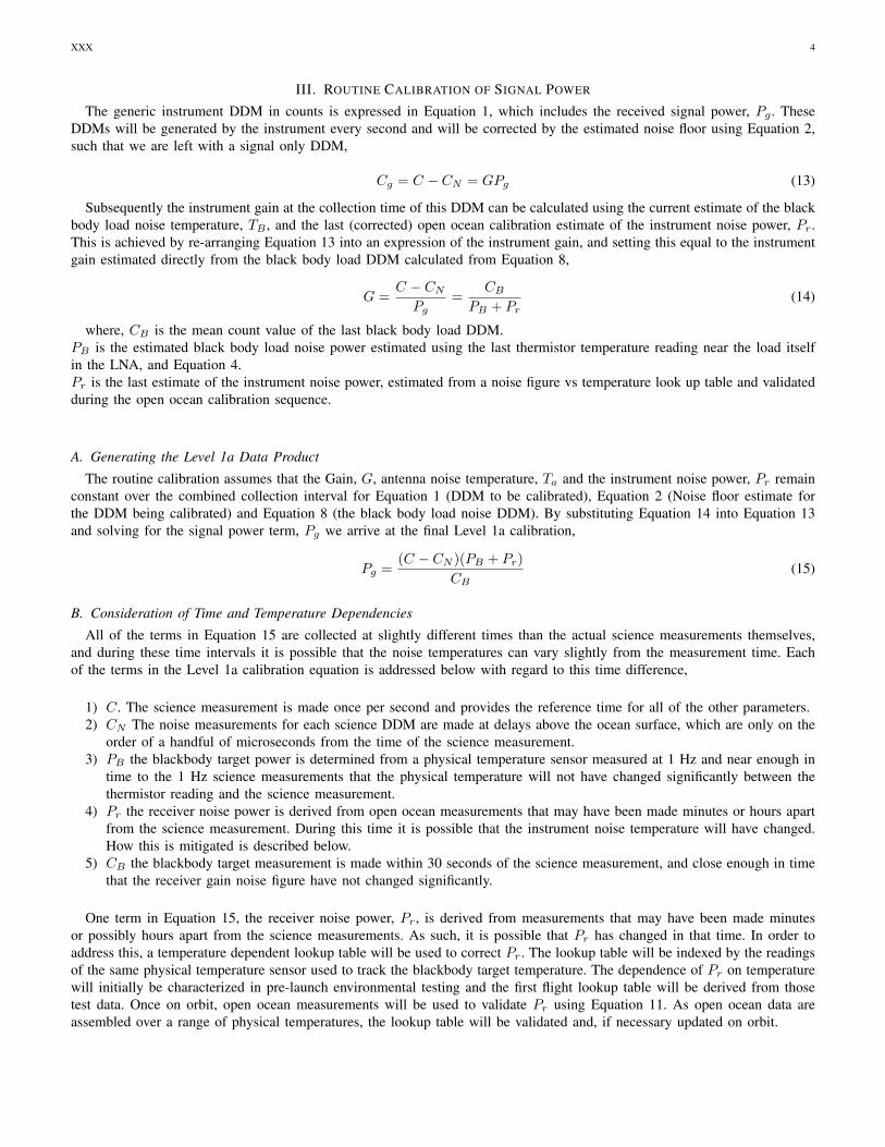
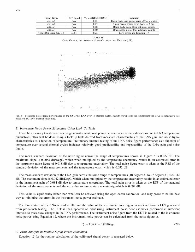
Fig. 3. Measured noise figure performance of the CYGNSS LNA over 13 thermal cycles. Results shown over the temperature the LNA is expected to seebased on S/C level thermal modelling.

B. Instrument Noise Power Estimation Using Look Up TableIt will be necessary to estimate the change in instrument noise power between open ocean calibrations due to LNA temperature

fluctuations. This will be done using a look up table derived from measured characteristics of the LNA gain and noise figurecharacteristics as a function of temperature. Preliminary thermal testing of the LNA noise figure performance as a function oftemperature over several thermal cycles indicates relatively good predictability and repeatability of the LNA gain and noisefigure.

The mean standard deviation of the noise figure across the range of temperatures shown in Figure 3 is 0.027 dB. Themaximum slope is 0.0088 dB/DegC, which when multiplied by the temperature uncertainty results in an estimated error inthe instrument noise figure of 0.018 dB due to temperature uncertainty. The total noise figure error is taken as the RSS of thestandard deviation of the measurements and the temperature error, which is 0.032 dB.

The mean standard deviation of the LNA gain across the same range of temperatures (10 degrees C to 27 degrees C) is 0.042dB. The maximum slope is 0.042 dB/DegC, which when multiplied by the temperature uncertainty results in an estimated errorin the instrument gain of 0.084 dB due to temperature uncertainty. The total gain error is taken as the RSS of the standarddeviation of the measurements and the error due to temperature uncertainty, which is 0.094 dB.

This value is significantly better than what can be achieved using the open ocean calibration, and may prove to be the bestway to minimize the errors in the instrument noise power estimate.

The temperature of the LNA is read at 1Hz and the value of the instrument noise figure is retrieved from a LUT generatedfrom pre-launch testing. The LUT is then updated on orbit using instrument noise floor estimates performed at sufficientintervals to track slow changes in the LNA performance. The instrument noise figure from the LUT is related to the instrumentnoise power using Equation 12, where the instrument noise power can be calculated from the noise figure as,

Pr = k(NF − 1)290BW (29)

C. Error Analysis in Routine Signal Power EstimationEquation 15 for the routine calculation of the calibrated signal power is repeated below,

XXX 8

Pg =(C − CN )(PB + Pr)

CB(30)

The total error in the estimate of the signal power, Pg , is the root sum square (RSS) of the individual errors contributed bythe independent terms of Equation 30, expressed as,

∆Pg =

[5∑

i=1

E2(pi)

]1/2(31)

where the partial derivatives of the individual errors terms can be expressed as,

E(pi) =

∣∣∣∣∣∂Pg

∂pi

∣∣∣∣∣∆pi (32)

The individual error quantities are defined as: p1 = C, p2 = CN , p3 = PB , p4 = Pr and p5 = CB . The 1-sigma uncertaintiesin these quantities are expressed as ∆pi. Using Equation 30 and Equation 32 to evaluate the partial derivative error terms weobtain,

E(C) =PB + Pr

CB∆C (33)

E(CN ) =PB + Pr

CB∆CN (34)

E(PB) =C − CN

CB∆PB (35)

E(Pr) =C − CN

CB∆Pr (36)

E(CB) =(C − CN )(PB + Pr)

C2B

∆CB (37)

where the error terms can be calculated from the following,

∆C: The error inherent in the Level 0 DDM’s from the instrument is due to the quantization error in the raw DDM bins. Fromthe CYGNSS DDM compression algorithm, each DDM bin will be quantized over a range of 9 bits, resulting in an error of 1

29 .

∆CN : The error in the estimate of the DDM noise floor (from DDM samples above the ocean surface) is a function of thenumber of noise samples taken and can be expressed as,

∆CN = std(~CN2

N ) (38)

Where ~CN2

N is a noise samples vector of length N2. Given 20 noise samples in every DDM Doppler row, a half of a fullDDM coresponds to 64 rows or 1280 samples.

∆PB can be calculated from Equation 25, ∆Pr is the root sum square errors from the open open calibration and ∆CB canbe calculated from Equation 27. Quantitative values for each or the error components listed above and the RSS total for bothwind retrieval regions are shown in Table III. The below 20 m/s wind analysis assumed a σ0 value of 20 dB, while the above20 m/s regions assumed a σ0 of 12 dB. Table III reflects that in order to accurately determine the DDM noise floor, CN , it isdesirable to have at least half a DDM of noise samples.

Table III shows the estimated L1a errors for the 20 m/s and below and the above 20 m/s wind speed cases. The estimatedσ0 for 20 m/s winds is 20 dB)

XXX 9

Error Term N1 = 2 DDMs, N2 = (52 rows), σ0 = 20 N1 = 2 DDMs, N2 = (52 rows), σ0 = 12 CommentE(C) 0.002 0.01 Quantization errorE(CN ) 0.03 0.14 Noise floor power error, countsE(PB) 0.01 0.01 Black body load power error ∆TB = 2 degE(Pr) 0.49 0.10 Instrument noise error, from open ocean calibrationE(CB) 0.04 0.04 Black body noise floor estimate, counts

Total RSS Error 0.49 0.17 Equations 17 and ??

TABLE IIIROUTINE L1A SIGNAL POWER CALIBRATION ERRORS (DB).

V. ZENITH ANTENNA CALIBRATION

The calibration of the zenith antenna is performed along the same general lines as the nadir antennas with a number ofimportant differences. These differences include,

1) The zenith antenna calibration load can’t be switched as often as the nadir antennas, as switching to the black bodycalibration load on the zenith channel will cause a navigation outage (and a corresponding science data outage) for upto 30 seconds.

2) The reference noise floor is not computed as noise samples in a DDM, but as the output of a separate noise channel.3) The reference noise floor is more susceptible to biases due to cross correlated power of other GNSS satellites in view.4) The signal powers are generated by the instrument as signal to noise ratio’s and not raw power in counts, requiring an

additional conversion step.5) The cold source reference antenna noise temperature is the deep space noise temperature (as opposed to the open ocean

noise temperature).

The slower black body calibration interval requires that the calibration algorithm relies more heavily on a well characterizedLNA noise figure and gain as a function of temperature to estimate changes to the zenith channel. Accurately determining thezenith LNA temperature performance, and limiting the gradient of the temperature fluctuations seen by the LNA are of criticalimportance to accurately determining the noise and signal power coming from the zenith antenna channel.

A. Zenith Black Body Load Calibration

The zenith channel instrument noise power is estimated as,

Pr =PDSCB − PBCDS

CDS − CB(39)

where PDS is the estimated deep space antenna noise power, CB is the black body load noise floor and CDS is the deepspace noise floor. The deep space noise power will be estimated using a model. The black body noise floor will only bemeasured on the satellite at long intervals (on the order of once per day). The instrument noise power calculated during thezenith black body calibration will be used to update the instrument noise and gain look up tables and track slow changes tothe LNA during the mission lifetime.

The LUT updates relating the LNA temperature (measured from thermistor in the LNA) to the instrument noise power willbe performed approximately every day.

The deep space antenna noise power relates to the deep space antenna noise temperature, TDS ,as follows,

PDS = kTDSBW (40)

B. Routine Instrument Zenith Gain Estimation

The instrument noise channels will continually provide an estimate of the deep space noise floor, which is a function of thedeep space noise power at the antenna and the instrument noise power, such that,

CDS = G(PDS + Pr

)(41)

From these continuous measurements it will be possible to calculate the instrument gain by re-arranging Equation 41 andsolving for the instrument gain as,

XXX 10

Error Term Error Estimate CommentE(Cz

l ) 0.00 Quantization errorE(Cz

N ) 0.03 Noise floor power errorE(PB) 0.01 Black body load power error ∆TB = 2 deg

E(PLUTr ) 0.037 Instrument noise error, from LUT

E(CLUTB ) 0.092 Black body noise floor estimate, from LUT

Total RSS Error 0.09 Equation 31

TABLE IVROUTINE ZENITH POWER L1A CALIBRATION ERRORS (DB).

G =

(PDS + PLUT

r

)CDS

(42)

where, PLUTr is calculated using a look up table relating the instrument noise figure to LNA temperature.

C. Direct Signal Power Estimation

The received signal power levels of the direct signals tracked by the navigation receiver can be expressed as,

Pl =(Cl − CN )(PB + PLUT

r )

CLUTB

(43)

where Pl is the received direct signal power for satellite l, PLUTr is the current estimate of the zenith channel instrument noise

power determined from a LUT of instrument noise power vs temperature, Cl is the direct signal plus noise value and CN isthe instantaneous zenith noise floor. PB is the black body load noise power, related directly to the black body load temperaturefrom Equation 23. Finally, CLUT

B is the black body noise floor estimated using the current estimate of the instrument gain(calculated using Equation 42) and an estimate of the instrument noise power from a LUT as a function of the black bodyload temperature using Equation 8.

The zenith antenna calibration must be performed without regular switching to the black body load calibration source. Thisrequires that both the noise figure and gain of the zenith channel are well modelled using look up tables. The gain of theinstrument can be tracked using the deep space noise floor (available continuously). The instrument noise power must beestimated using a table, which will be periodically updated using an approximately daily black body load calibration.

D. Error Analysis of Zenith Antenna Calibration

The errors in the zenith antenna signal power calibration are summarized below,1) The quantization error E(Cl) in the noise floor and signal channel measurements will be negligible due to the fact that

these values are estimated by dedicated channels in the instrument and sent to the ground with sufficient resolution tocapture the value entirely.

2) The reference noise floor E(CN ) is also computed by a dedicated channel on the instrument. The errors are againexpected to be small, due only to possible cross correlation power from other GNSS satellites slightly biasing the noisefloor channels.

3) The black body load power E(PB) error is a direct function of the temperature and is expected to be similar to that ofthe nadir antenna calibration.

4) The error in the instrument power LUT E(PLUTr ) will be generated using LNA noise figure test data. This error includes

an additional small error due to the ageing of the LNA, which will cause slight differences between the on-orbit valuesand those in the current LUT. The LUT will be updated using periodic deep space instrument gain and noise figurecalibrations on-orbit.

5) The error in the black body noise floor LUT E(CLUTB ) will be estimated using LNA gain test data for the instrument

power and the continuos estimate of the instrument gain. As with the instrument noise LUT, this table will also containa small error due to LNA ageing and will be updated at periodic intervals on-orbit.

The errors in the instrument noise figure and gain look up tables is estimated to be on the order of 0.01 dB and has beenincluded in the error analysis shown in Table IV.

XXX 11

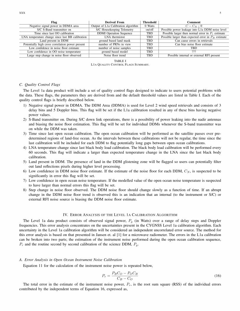
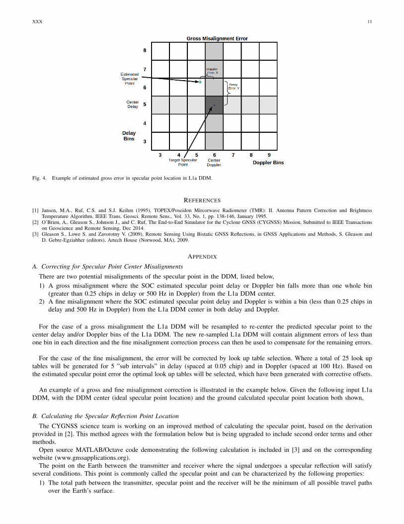
Fig. 4. Example of estimated gross error in specular point location in L1a DDM.

REFERENCES

[1] Jansen, M.A., Ruf, C.S. and S.J. Keihm (1995), TOPEX/Poseidon Mircorwave Radiometer (TMR): II. Antenna Pattern Correction and BrightnessTemperature Algorithm, IEEE Trans. Geosci. Remote Sens., Vol. 33, No. 1, pp. 138-146, January 1995.

[2] O’Brien, A., Gleason S., Johnson J., and C. Ruf, The End-to-End Simulator for the Cyclone GNSS (CYGNSS) Mission, Submitted to IEEE Transactionson Geoscience and Remote Sensing, Dec 2014.

[3] Gleason S., Lowe S. and Zavorotny V. (2009), Remote Sensing Using Bistatic GNSS Reflections, in GNSS Applications and Methods, S. Gleason andD. Gebre-Egziabher (editors), Artech House (Norwood, MA), 2009.

APPENDIX

A. Correcting for Specular Point Center Misalignments

There are two potential misalignments of the specular point in the DDM, listed below,1) A gross misalignment where the SOC estimated specular point delay or Doppler bin falls more than one whole bin

(greater than 0.25 chips in delay or 500 Hz in Doppler) from the L1a DDM center.2) A fine misalignment where the SOC estimated specular point delay and Doppler is within a bin (less than 0.25 chips in

delay and 500 Hz in Doppler) from the L1a DDM center in both delay and Doppler.

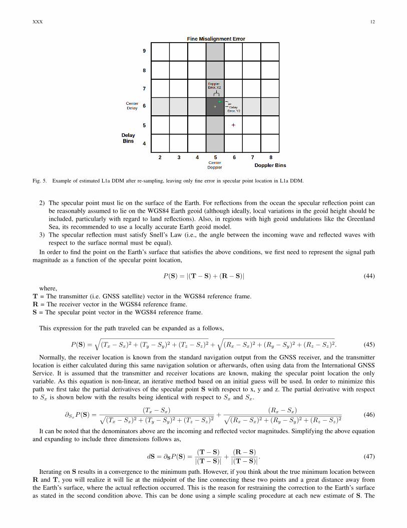
For the case of a gross misalignment the L1a DDM will be resampled to re-center the predicted specular point to thecenter delay and/or Doppler bins of the L1a DDM. The new re-sampled L1a DDM will contain alignment errors of less thanone bin in each direction and the fine misalignment correction process can then be used to compensate for the remaining errors.

For the case of the fine misalignment, the error will be corrected by look up table selection. Where a total of 25 look uptables will be generated for 5 ”sub intervals” in delay (spaced at 0.05 chip) and in Doppler (spaced at 100 Hz). Based onthe estimated specular point error the optimal look up tables will be selected, which have been generated with corrective offsets.

An example of a gross and fine misalignment correction is illustrated in the example below. Given the following input L1aDDM, with the DDM center (ideal specular point location) and the ground calculated specular point location both shown,

B. Calculating the Specular Reflection Point Location

The CYGNSS science team is working on an improved method of calculating the specular point, based on the derivationprovided in [2]. This method agrees with the formulation below but is being upgraded to include second order terms and othermethods.

Open source MATLAB/Octave code demonstrating the following calculation is included in [3] and on the correspondingwebsite (www.gnssapplications.org).

The point on the Earth between the transmitter and receiver where the signal undergoes a specular reflection will satisfyseveral conditions. This point is commonly called the specular point and can be characterized by the following properties:

1) The total path between the transmitter, specular point and the receiver will be the minimum of all possible travel pathsover the Earth’s surface.

XXX 12

Fig. 5. Example of estimated L1a DDM after re-sampling, leaving only fine error in specular point location in L1a DDM.

2) The specular point must lie on the surface of the Earth. For reflections from the ocean the specular reflection point canbe reasonably assumed to lie on the WGS84 Earth geoid (although ideally, local variations in the geoid height should beincluded, particularly with regard to land reflections). Also, in regions with high geoid undulations like the GreenlandSea, its recommended to use a locally accurate Earth geoid model.

3) The specular reflection must satisfy Snell’s Law (i.e., the angle between the incoming wave and reflected waves withrespect to the surface normal must be equal).

In order to find the point on the Earth’s surface that satisfies the above conditions, we first need to represent the signal pathmagnitude as a function of the specular point location,

P (S) = |(T− S) + (R− S)| (44)

where,T = The transmitter (i.e. GNSS satellite) vector in the WGS84 reference frame.R = The receiver vector in the WGS84 reference frame.S = The specular point vector in the WGS84 reference frame.

This expression for the path traveled can be expanded as a follows,

P (S) =√

(Tx − Sx)2 + (Ty − Sy)2 + (Tz − Sz)2 +√

(Rx − Sx)2 + (Ry − Sy)2 + (Rz − Sz)2. (45)

Normally, the receiver location is known from the standard navigation output from the GNSS receiver, and the transmitterlocation is either calculated during this same navigation solution or afterwards, often using data from the International GNSSService. It is assumed that the transmitter and receiver locations are known, making the specular point location the onlyvariable. As this equation is non-linear, an iterative method based on an initial guess will be used. In order to minimize thispath we first take the partial derivatives of the specular point S with respect to x, y and z. The partial derivative with respectto Sx is shown below with the results being identical with respect to Sx and Sx.

∂SxP (S) =(Tx − Sx)√

(Tx − Sx)2 + (Ty − Sy)2 + (Tz − Sz)2+

(Rx − Sx)√(Rx − Sx)2 + (Ry − Sy)2 + (Rz − Sz)2

(46)

It can be noted that the denominators above are the incoming and reflected vector magnitudes. Simplifying the above equationand expanding to include three dimensions follows as,

dS = ∂SP (S) =(T− S)

|(T− S)|+

(R− S)

|(T− S)|. (47)

Iterating on S results in a convergence to the minimum path. However, if you think about the true minimum location betweenR and T, you will realize it will lie at the midpoint of the line connecting these two points and a great distance away fromthe Earth’s surface, where the actual reflection occurred. This is the reason for restraining the correction to the Earth’s surfaceas stated in the second condition above. This can be done using a simple scaling procedure at each new estimate of S. The

XXX 13

radius of the Earth according to the WGS84 model can be calculated as a simple function of the specular point estimate zcoordinate (i.e., latitude) as follows,

r = aWGS84

√1− e2WGS84

1− (e2WGS84 + cos(λ))(48)

with λ = sin( Sz

|S| )where aWGS84 = 6378137 meters and eWGS84= 0.08181919084262 are the semi-major axis and the eccentricity of the

WGS84 Earth geoid, respectively. The point on the Earth’s surface that satisfies the three conditions listed above is then solvedfor iteratively, using the equations below. A correction gain K has been added to quicken the convergence, considering thatthe initial guess for the location of S(for example, the sub-receiver Earth surface point) will be a great distance from the finalsolution as follows.

Stemp = (S +Ks) (49)

where s = ∂S|∂S| is the directional unit vector for the correction.

This intermediate value is then converted to a unit vector and scaled by the Earth radius, giving us the new estimate for Sto be used during the next iteration,

S = rStemp = rStemp

|Stemp|. (50)

The specular point can be considered found when the difference between the old and new values of S falls below a specifiedtolerance after several iterations. Finally, we can test the third condition listed above, that Snells law is satisfied with respect tothe incoming and reflected wave directions. This complete procedure is fairly easy to implement in any mathematical scriptinglanguage.

C. Estimating the Specular Point Doppler Frequency

The Doppler frequency of the reflected signal at the specular reflection point can be accurately determined using knownpositions and velocities of the transmitter and receiver and the position of the specular point. The general formula for thecalculation of Doppler frequency is shown below with an important addition. In the GNSS case the Doppler includes anadditional term representing the rate of the receiver clock drift.

In the case of a surface reflection three points are involved; The transmitter (Tx, Tv), the receiver (Rx, Rv), and the specularreflection point (Sx) on the Earth’s surface. This necessitates that the calculation be split into two parts, the component dueto the receiver velocity, the component due to the transmitter velocity and the contribution due to the receiver clock drift.

D = DRx +DTx +Dclk (51)

DRx=−Rv · Rx−Sx

|Rx−Sx|f

c(52)

DTx=−Tv · Tx−Sx

|Tx−Sx|f

c(53)

Where f is the signal frequency (1575.42e6 Hz for GPS L1), c is the speed of light in a vacuum (2.99792458e8 m/s) andDclk is the Doppler contribution due to the receiver clock drift b. The receiver clock drift is normally estimated during thenavigation solution in units of m/s and can be converted to a frequency as, Dclk = bf

c . The clock drift of the transmittingsatellite is very small and is not considered.

It can be observed that when using the above equation the velocity of the specular point, or any point on the surface, is zeroin an Earth Centered Earth Fixed (ECEF) reference frame such as that of the World Geodetic System 1984 (WGS84). Thiscalculation can be performed around the surface region of the specular reflection point to map the scattered signal frequencyover the glistening zone.

XXX 14

D. Estimating the Specular Point Code Phase, Relative Calculation

It is possible to estimate the delay of the specular reflection point using the direct signal delay as a relative reference.

φrelreflected(t) = φdirect +mod(PS −Rd

mchip, 1023) (54)

PS is the total path length from the transmitter to the specular point to the receiver. Rd is the path length from the transmitterto the receiver directly. For the case of the CYGNSS DDM, the above results needs to be corrected for two additional factor.These are a) The number of samples between the 1Hz GPS epoch when the the above calculation is valid and the DDM timewhich is offset by a known number of samples and b) any additional instrument delays. The final expression for the relativedelay of the specular point is,

φrelreflected(tDDM ) = φrelreflected(t) + φsamples + φHW (55)

Where,

φsamples = SDCONsamples

SI(56)

SDCO = SCA +D

mchip/λ(57)

SI is the DDM sampling rate of the instrument, Nsamples is the number of samples between the 1Hz epoch and the DDMintegration start time. SDCO is the actual code rate at Doppler D. SCA is the nominal C/A code code rate. λ is the GPS C/Acode wavelength. φHW is to account for all hardware induced code phase delays.

E. Estimating the Specular Point Code Phase, Absolute Calculation

In absolute terms, the code phase of the received GPS signal is a function of the GPS time, the locations of the transmitter,receiver and reflection point as well as the clock errors of the transmitting satellite and sampling GPS receiver. These biasesare relative to the start of the GPS C/A code transmission time and allow us to link the received code phase to the code phasestart time on the satellite. The absolute code phases of the direct and reflected signals can be calculated as follows,

φdirect(t) = 1023− 1023mod(Rd(tDDM )

1023mchip, 1)− mod(tDDM , 0.001)c

mchip+mod(Tbias(tDDM ), 0.001)c

mchip+ φHW (58)

φabsreflected(t) = 1023− 1023mod(PS(tDDM )

1023mchip, 1)− mod(tDDM , 0.001)c

mchip+mod(Tbias(tDDM ), 0.001)c

mchip+ φHW (59)

where: Rd is the direct path length from the transmitter to the receiver, PS is the total path length from the transmitter tothe specular point to the receiver, mchip is the length of 1 GPS L1 C/A code chip, Tbias is the clock bias of the transmittingsatellite, 1023 is the code length in number of chips and c is the speed of light. All values used in this formula must be validat time tDDM , which is the GPS time stamp at the start of the DDM integration. All of the time terms need to be computedmodulo 1 ms, and distance terms modulo 1 complete code repeat period distance (1023mchip) corresponding to the code repeatperiod of the transmitted signal. Lastly, if the final value of the code phase is less than 0, simply add 1023 to the result.