1 | P a g e

Cylinder in Cross Flow— Comparing CFD Simulations w/ Experiments

Theoretical Drag Coefficients

Examples of cylindrical objects in cross flow (i.e. with the freestream flow direction normal to the

cylinder axis) include wind and water flow over offshore platform supports, flow across pipes or heat

exchanger tubes, and wind flow over power and phone lines. The drag coefficient for such an object

depends strongly on the behavior of the fluid around the cylinder (see Figure 1). For example,

depending on the Reynolds number, DURe , the flow pattern near the cylinder can vary

significantly, where and are the fluid density and viscosity, U is the upstream velocity, and D is the

cylinder diameter. For low velocities (i.e. ReD < 5), the flow around the cylinder is unseparated; whereas

for 5 < ReD < 40, two stationary eddies form immediately downstream of the cylinder. For higher

velocities (i.e. ReD > 40), an unsteady wake flow occurs, the width and nature of which depends on the

Reynolds number.

Fig. 1 Different characteristic flow regimes manifested by a cylinder in cross flow [1]

2 | P a g e

Fig. 2 Drag coefficient as a function of Reynolds number for a smooth circular cylinder

(Adapted from Ref. [1])

In Figure 2, the theoretical drag coefficient associated with these different flow regimes is plotted

for a smooth circular cylinder as a function of Reynolds number. For example, for the case of no

separation (i.e. Case A), the drag coefficient is a little less than 50. For the case of a laminar boundary

layer with a wide turbulent wake (i.e. Case D), the drag coefficient is approximately 1.6 whereas for the

case of a turbulent boundary layer with a narrower turbulent wake, the drag coefficient is reduced. In this

case, the drag coefficient is approximately. 0.30. So why is this?

To answer this question, let’s consider how the flow behaves around the cylinder. Over the

forward portion of the cylinder, the surface pressure decreases from the stagnation point toward the

shoulder. In this region, the boundary layer (i.e. the thin region adjacent to the surface where viscous

shear effects are important) develops under a favorable pressure gradient (i.e. 0 P ). In this region

the net pressure force on a fluid element in the direction of the flow is sufficient to overcome the resisting

shear force. Thus, the motion of the element in the flow direction is maintained. However, the surface

pressure eventually reaches a minimum and then begins increasing toward the rear of the cylinder. Thus,

the boundary layer in this downstream region experiences an adverse pressure gradient (i.e. 0 P ).

Since the pressure increases in the flow direction, a fluid element in the boundary layer experiences a net

pressure force opposite to its direction of motion. At some point, the momentum of the fluid element will

be insufficient to carry it into regions of increasing pressure. Here, the fluid adjacent to the solid surface is

brought to rest, and flow separation from the surface occurs. In the case of a turbulent boundary layer,

3 | P a g e

there is more momentum associated with the fluid. Thus, separation occurs farther back on the cylinder.

As a result, the wake region behind the cylinder is considerably narrower and there is a considerable drop

in pressure drag (with only a slight increase in the friction drag).

This is actually the reason why a golf ball is dimpled. The surface roughness associated with the dimples

facilitates an earlier transition from a laminar boundary layer to a turbulent boundary layer (i.e. at smaller

Reynolds numbers). The resulting reduction in drag permits the golf ball to be hit greater distances.

Comparing ANSYS Fluent Simulations to Experiments

Now, let’s consider two of these cases— namely, Case A and Case D. In both cases, we will compare the

theoretical value (from Fig. 1) with the experimental value and the computationally determined value

using ANSYS Fluent.

Case A— Creeping Flow (ReD 0.15)

As we indicated earlier, the theoretical CD value for Case A is approximately 45 - 50. This compares

quite favorably with the value attained using ANSYS Fluent which was 43.7 (shown in Fig. 4). A plot of

the velocity magnitude is shown in Figure 3. Due to the low velocities, there is no flow separation, and as

might be expected, the regions of highest velocity occur along the sides of the cylinder where the fluid

accelerates to move around the object. Unfortunately, the speeds involved here are too low to be tested in

the MME wind tunnel. Thus, no experimental CD value is available for comparison for this case.

Fig. 3 Velocity Magnitude Contours for Case A

4 | P a g e

Fig. 4 Velocity vectors around the cylinder and simulated drag coefficient for Case A

Case D— Wide Turbulent Wake (ReD 20,000 40,000)

As we indicated earlier, the theoretical CD value for Case D is approximately 1.6. This compares well

with the value attained using ANSYS Fluent which was 1.524 (shown in Fig. 5). This value is simply the

result of adding the pressure drag (i.e. 1.498) to the viscous (or, friction) drag component (i.e. 0.026).

Clearly in this case, the pressure drag is more dominant. The experimentally determined drag coefficient

(CD = 1.70 1.72) is shown in Fig. 6 for a slightly higher Reynolds number (i.e. ReD = 48,200). All three

values compare quite favorably.

5 | P a g e

Fig. 5 Computationally Determined CD for Case D

Fig. 6 Experimentally Determined CD for Case D (slightly higher ReD)

Object D (mm) T1

Vel

(m/s)

Patm

(mmHg)

T1

(Celsius)

T1

(K)

mu air

(Pa-s)

rho air

(kg/m3) Re

Cylinder 88.9 23.33 8.55 746 23.33 296.48 1.84E-05 1.16791 48245.79

Trapezoidal Simpson

Theta (deg) Theta (rad) Ps-P1 (H20) Ps-P1 (Pa) Cp Integrand Weight Int*Wt Weight Int*Wt

0 0 0.063191732 15.724631 0.368356925 0.368356925 1 0.368357 1 0.368357

10 0.1745329 0.053649902 13.350242 0.312735741 0.307984584 2 0.615969 4 1.231938

20 0.3490659 -0.01595052 -3.969128 -0.092978696 -0.087371393 2 -0.17474 2 -0.17474

30 0.5235988 -0.1104126 -27.47507 -0.643616559 -0.557388283 2 -1.11478 4 -2.22955

40 0.6981317 -0.22920736 -57.03596 -1.336094372 -1.02350767 2 -2.04702 2 -2.04702

50 0.8726646 -0.36159261 -89.97871 -2.107793829 -1.354863799 2 -2.70973 4 -5.41946

60 1.0471976 -0.46394857 -115.449 -2.70444666 -1.352223216 2 -2.70445 2 -2.70445

70 1.2217305 -0.48276774 -120.1319 -2.814147289 -0.962494997 2 -1.92499 4 -3.84998

80 1.3962634 -0.4508667 -112.1937 -2.628189898 -0.45638039 2 -0.91276 2 -0.91276

90 1.5707963 -0.42651367 -106.1337 -2.486231353 -6.66183E-08 2 -1.3E-07 4 -2.7E-07

100 1.7453293 -0.43103027 -107.2576 -2.512559504 0.436301498 2 0.872603 2 0.872603

110 1.9198622 -0.42108154 -104.7819 -2.454566414 0.839511209 2 1.679022 4 3.358045

120 2.0943951 -0.45676676 -113.6618 -2.662582527 1.331291258 2 2.662583 2 2.662583

130 2.268928 -0.44812012 -111.5102 -2.612179535 1.679076584 2 3.358153 4 6.716306

140 2.443461 -0.45607503 -113.4897 -2.658550288 2.036567756 2 4.073136 2 4.073136

150 2.6179939 -0.42600505 -106.0071 -2.483266471 2.150571876 2 4.301144 4 8.602288

160 2.7925268 -0.43094889 -107.2373 -2.512085123 2.36058785 2 4.721176 2 4.721176

170 2.970597 -0.51200358 -127.407 -2.9845687 2.941041247 2 5.882082 4 11.76416

180 3.1415927 -0.434611 -108.1486 -2.533432273 2.533432273 1 2.533432 1 2.533432

Cd 1.699881 1.720084

6 | P a g e

A plot of the velocity magnitude for Case D (as predicted from the CFD simulation) is shown in Figure 7.

In this image, the stagnation region at the front of the cylinder, and the wide wake region behind the

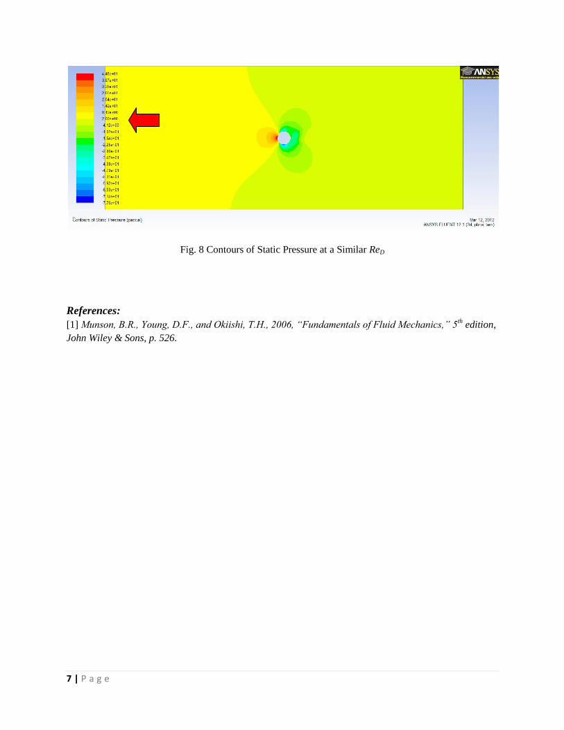
cylinder can be clearly observed with defined regions of recirculation. It should also be noted in Fig. 8

that (for a similar Reynolds number) the static pressure begins showing negative values at angles of

approx. 30-40 (as measured from the front of the cylinder) which agrees well with the negative surface

pressure difference measurements shown in Fig. 6. Here, negative surface pressure measurements were

recorded in the wind tunnel at approx. 20-30.

Fig. 7 Contours of Velocity Magnitude and Velocity Vectors for Case D

7 | P a g e

Fig. 8 Contours of Static Pressure at a Similar ReD

References:

[1] Munson, B.R., Young, D.F., and Okiishi, T.H., 2006, “Fundamentals of Fluid Mechanics,” 5th edition,

John Wiley & Sons, p. 526.