cylinder pressure and ionization current modeling for spark ignited
TRANSCRIPT
Linkoping Studies in Science and TechnologyThesis No. 962
Cylinder Pressure and Ionization
Current Modeling for Spark
Ignited Engines
Ingemar Andersson
Division of Vehicular Systems
Department of Electrical Engineering
Linkopings Universitet, SE–581 83 Linkoping, Sweden
http://www.vehicular.isy.liu.se/
Email: [email protected]
Linkoping 2002
Cylinder Pressure and Ionization Current Modeling for SparkIgnited Engines
c© 2002 Ingemar Andersson
Department of Electrical Engineering,
Linkopings Universitet,
SE–581 83 Linkoping,
Sweden.
ISBN 91-7373-379-2ISSN 0280-7971
LiU-TEK-LIC-2002:35
i
Abstract
Engine management systems (EMS) need feedback on combustion performanceto optimally control internal combustion engines. Ion sensing is one of thecheapest and most simple methods for monitoring the combustion event in aspark ignited engine, but still the physical processes behind the formation ofthe ionization current are not fully understood.
The goal here is to investigate models for ionization currents and make aconnection to combustion pressure and temperature. A model for the thermalpart of an ionization signal is presented that connects the ionization currentto cylinder pressure and temperature. One strength of the model is that itafter calibration has only two free parameters, burn angle and initial kerneltemperature. By fitting the model to a measured ionization signal it is possi-ble to estimate both cylinder pressure and temperature, where the pressure isestimated with good accuracy. The parameterized ionization current model iscomposed by four parts; a thermal ionization model, a model for formation ofnitric oxide, a combustion temperature model and a cylinder pressure function.The pressure function is an empirical function design where the parameters havephysical meaning and the function has the main properties of a solution to thecylinder pressure differential equations. The sensitivity of the ionization currentmodel to combustion temperature and content of nitric oxide is investigated tounderstand the need of sub-model complexity.
Two main results are that the pressure model itself well captures the be-havior of the cylinder pressure, and that the parameterized ionization currentmodel can be used with an ionization current as input and work as a virtualcylinder pressure sensor and a combustion analysis tool. This ionization cur-rent model not only describes the connection between the ionization currentand the combustion process, it also offers new possibilities for EMS to controlthe internal combustion engine.

ii
iii
Acknowledgements
This work was performed in the supervision of Professor Lars Nielsen at Vehic-ular Systems, Dept. of Electrical Engineering, Linkoping University, Sweden,and in collaboration with Mecel AB, Amal, Sweden.
I would like to thank Mecel AB and especially Jan Nytomt and AndersGoras for their support and encouragement during the four years of this work.Also, ECSEL (Ecsellence center in Computer science and Systems Engineeringin Linkoping) deserves acknowledgement for funding the project.
A special thanks is directed to Lars Eriksson for his indefatigable enthusiasmin my research and the numerous inspiring discussions along the way. I wouldlike to thank Professor Lars Nielsen for his supervision and especially for hisknowledge about presentation technique and manners, and Erik Frisk, who hasgiven invaluable support in the djungle of LATEX and a number of UNIX basedtools and also the inspiring discussions at Snoddas’ about the meaning of life.
I would also like to thank the group of Vehicular Systems for over-all inter-esting discussions and joyful fellowship. My hosts during the almost four yearsdeserve special thanks; Maj-Lis Vaag, Lars Eriksson and Jan Brugard.
Thank you all for helping me completing this work.
Linkoping, May 2002
Ingemar Andersson

iv
Contents
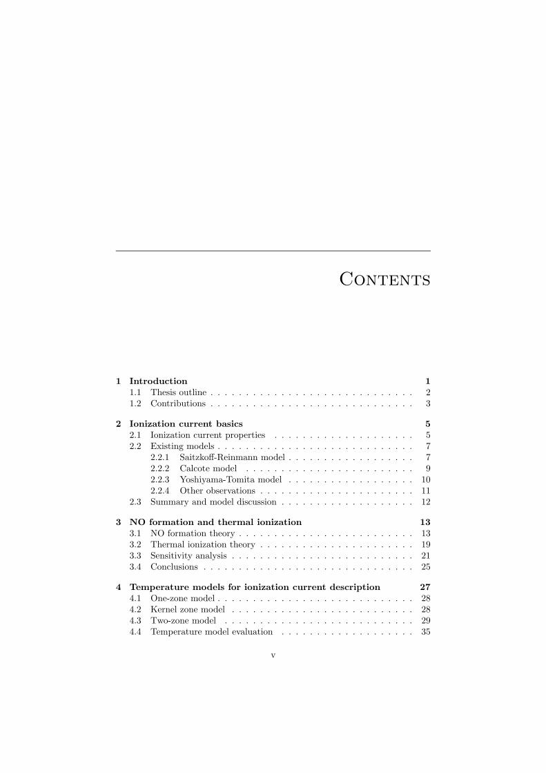
1 Introduction 11.1 Thesis outline . . . . . . . . . . . . . . . . . . . . . . . . . . . . . 21.2 Contributions . . . . . . . . . . . . . . . . . . . . . . . . . . . . . 3
2 Ionization current basics 52.1 Ionization current properties . . . . . . . . . . . . . . . . . . . . 52.2 Existing models . . . . . . . . . . . . . . . . . . . . . . . . . . . . 7
2.2.1 Saitzkoff-Reinmann model . . . . . . . . . . . . . . . . . . 72.2.2 Calcote model . . . . . . . . . . . . . . . . . . . . . . . . 92.2.3 Yoshiyama-Tomita model . . . . . . . . . . . . . . . . . . 102.2.4 Other observations . . . . . . . . . . . . . . . . . . . . . . 11
2.3 Summary and model discussion . . . . . . . . . . . . . . . . . . . 12
3 NO formation and thermal ionization 133.1 NO formation theory . . . . . . . . . . . . . . . . . . . . . . . . . 133.2 Thermal ionization theory . . . . . . . . . . . . . . . . . . . . . . 193.3 Sensitivity analysis . . . . . . . . . . . . . . . . . . . . . . . . . . 213.4 Conclusions . . . . . . . . . . . . . . . . . . . . . . . . . . . . . . 25
4 Temperature models for ionization current description 274.1 One-zone model . . . . . . . . . . . . . . . . . . . . . . . . . . . . 284.2 Kernel zone model . . . . . . . . . . . . . . . . . . . . . . . . . . 284.3 Two-zone model . . . . . . . . . . . . . . . . . . . . . . . . . . . 294.4 Temperature model evaluation . . . . . . . . . . . . . . . . . . . 35
v
vi
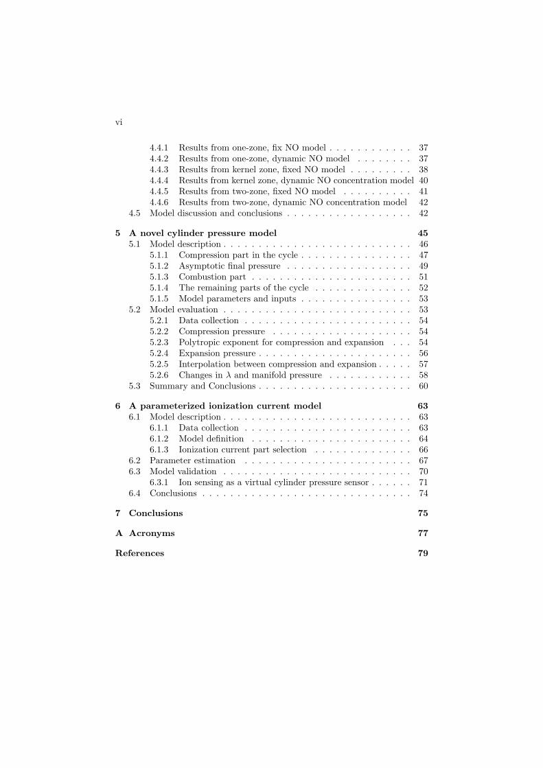
4.4.1 Results from one-zone, fix NO model . . . . . . . . . . . . 374.4.2 Results from one-zone, dynamic NO model . . . . . . . . 374.4.3 Results from kernel zone, fixed NO model . . . . . . . . . 384.4.4 Results from kernel zone, dynamic NO concentration model 404.4.5 Results from two-zone, fixed NO model . . . . . . . . . . 414.4.6 Results from two-zone, dynamic NO concentration model 42
4.5 Model discussion and conclusions . . . . . . . . . . . . . . . . . . 42
5 A novel cylinder pressure model 455.1 Model description . . . . . . . . . . . . . . . . . . . . . . . . . . . 46
5.1.1 Compression part in the cycle . . . . . . . . . . . . . . . . 475.1.2 Asymptotic final pressure . . . . . . . . . . . . . . . . . . 495.1.3 Combustion part . . . . . . . . . . . . . . . . . . . . . . . 515.1.4 The remaining parts of the cycle . . . . . . . . . . . . . . 525.1.5 Model parameters and inputs . . . . . . . . . . . . . . . . 53
5.2 Model evaluation . . . . . . . . . . . . . . . . . . . . . . . . . . . 535.2.1 Data collection . . . . . . . . . . . . . . . . . . . . . . . . 545.2.2 Compression pressure . . . . . . . . . . . . . . . . . . . . 545.2.3 Polytropic exponent for compression and expansion . . . 545.2.4 Expansion pressure . . . . . . . . . . . . . . . . . . . . . . 565.2.5 Interpolation between compression and expansion . . . . . 575.2.6 Changes in λ and manifold pressure . . . . . . . . . . . . 58
5.3 Summary and Conclusions . . . . . . . . . . . . . . . . . . . . . . 60
6 A parameterized ionization current model 636.1 Model description . . . . . . . . . . . . . . . . . . . . . . . . . . . 63
6.1.1 Data collection . . . . . . . . . . . . . . . . . . . . . . . . 636.1.2 Model definition . . . . . . . . . . . . . . . . . . . . . . . 646.1.3 Ionization current part selection . . . . . . . . . . . . . . 66
6.2 Parameter estimation . . . . . . . . . . . . . . . . . . . . . . . . 676.3 Model validation . . . . . . . . . . . . . . . . . . . . . . . . . . . 70
6.3.1 Ion sensing as a virtual cylinder pressure sensor . . . . . . 716.4 Conclusions . . . . . . . . . . . . . . . . . . . . . . . . . . . . . . 74
7 Conclusions 75
A Acronyms 77
References 79
1
Introduction
Internal combustion engines have been a major power source throughout thehistory of ground vehicles. Since the oil crisis in the 1970’s the focus for enginedevelopers have moved to fuel economy and emission reduction. The introduc-tion of electronic ignition and fuel injection systems in the 1980’s have given theengineers far more capability of engine control than before. The limitation inengine control development lies in the available information about the controlledprocess; the combustion.
Fuel economy drives the development of efficiency of the engine. This in-cludes optimal ignition timing and fuel amount for a given operating condition.Emission reduction drives the development of air-fuel ratio control, misfire de-tection and purge control. Oxygen sensors mounted in the exhaust pipe providea possibility for closed loop air-fuel ratio control and piezo-electric knock sensorsmounted on the engine block, for closed loop knock control, but the need forsupervising the combustion process itself increases constantly. Three methodsexist for combustion monitoring;
• cylinder pressure sensing
• ionization current sensing
• optical instruments
Optical methods include TV cameras or lasers targeting a transparent part inthe cylinder head or wall. This equipment is expensive and only suitable forlaboratory work. Cylinder pressure sensors can be mounted in the cylinder headto measure the pressure development during combustion. Most of the commonly
2 Chapter 1. Introduction
used combustion quality measures are related to the cylinder pressure. Thepressure sensor is currently only used in laboratory environments due to costand lifetime performance, but progress is made to find a sensor suitable to bemounted in future engine management systems (EMS). The only one of thethree mentioned sensing methods that is used in production EMS today is theionization current sensor. For spark ignited engines the spark plug is usedas sensor together with some measurement electronics added to the ignitionsystem. It is a relatively cheap method for combustion monitoring and othersensors can be replaced. The use of ion sensing in modern EMS is restricted toknock and misfire detection but engine developers start to see a need for othercombustion information, such as air-fuel ratio, torque, combustion stability andlocation of peak pressure. Research in the area aims to find the requestedinformation in the ionization current and the results are promising. Still, thereis much work left to explain and understand the information hidden in theionization current. This thesis will add a piece to that work.
1.1 Thesis outline
Chapter 2 presents a survey of earlier suggested models for ionization currentwith the basic thoughts and assumptions and, in the case they were presented,the equations for the model.
One model approach, by Saitzkoff and Reinmann, considers the second peakof the ionization current. It is used as the ionization base in the rest of themodeling work in the thesis. In Chapter 3 the ionization model is investigatedin more detail to understand the physical processes. A central part here isthe thermal ionization of nitric oxide, NO. NO is a combustion product whencarbon based fuel burns in air. The formation of NO is dependent of combus-tion temperature and the content of NO in the combusted gas is not constantthrough the combustion. The impact of dynamic or reaction rate controlled NOformation is studied.
The thermal ionization makes the combustion temperature an importantparameter. The description of the combustion temperature depends on thechosen combustion model. Chapter 4 investigates three different combustionmodel approaches in the sense of how they can help to explain the amplitudeand position of the ionization current.
Chapter 5 presents a parameterized model for cylinder pressure. The modelis not written in the traditional form of a differential equation, but as an explicitfunction of crank angle and measurable inputs of the combustion process. Thischapter was presented as a separate paper at SAE 2001 World Congress, SAE-2001-01-0371.
Finally, Chapter 6 puts the pieces from Chapters 3 - 5 together in one modelto connect cylinder pressure and ionization current. The model is composed bythe explicit pressure model, a kernel zone combustion model for temperaturecalculation, a dynamic NO formation model and a model for thermal ionization.
1.2. Contributions 3
A validation of the model is presented. Certain attention is given to how wellthe model describes the cylinder pressure based on the ionization current.
1.2 Contributions
The first two contributions are the investigation of the Saitzkoff-Reinmann ion-ization model properties and how important the models of NO formation andcombustion temperature are.
The main contributions lie in Chapters 5 and 6 which describe the devel-opment of a parameterized pressure function and the parameterized ionizationcurrent model. The parameterized cylinder pressure function presents an empir-ical solution with physically interpretable parameters to the pressure differentialequations.
The parameterized ionization current model describes the ionization currentwith only two free parameters that handle shift in both ignition timing andair-fuel ratio. One of the parameters is the total burn angle of the combustion,which here is possible to estimate. The model can use a measured ionizationcurrent as input and calculate the cylinder pressure with good performance.The modeling work altogether presents a virtual pressure sensor based on mea-surement of ionization current.

4 Chapter 1. Introduction
2
Ionization current basics
2.1 Ionization current properties
The combustion in a spark ignited (SI) engine normally starts with a sparkdischarge in the spark plug. A flame develops and travels from the spark pluglocation out to the cylinder walls as it consumes the air-fuel mixture. The chem-ical reactions and the raised temperature in the flame front produce free chargesthrough various ionization processes. The amount of free charges is small butmeasurable (Reinmann, 1998). By applying a voltage to the spark gap after thespark has vanished, the free charge will form a current, the ionization currentor ion current. The technology for measuring the ionization current is calledion sense. Figure 2.1 shows an symbolic ion sense system. The combustiongenerates free charge, e-. An outer measurement circuit provides the measure-ment voltage from a capacitor. The current I flows through the circuit and thecurrent equivalent voltage U ion is measured over the resistor R.
Ion sensing has been a hot topic in recent years concerning measurementtechniques and its possible applications (Nielsen and Eriksson, 1998; Asanoet al., 1998; Auzins et al., 1995; Balles et al., 1998; Collings et al., 1991; Daniels,1998; Forster et al., 1999; Hellring et al., 1999; Lee and Pyko, 1995; Shimasakiet al., 1993; Andersson and Eriksson, 2000). More theoretical investigations,concerning physical and chemical modeling, have been performed and reportedby Saitzkoff et al. (1997), Reinmann et al. (1998) and Wilstermann (1999).
The ionization current has a characteristic shape. One proposal divides theion current in three parts, the ignition phase, the flame front phase and thepost-flame phase (Eriksson et al., 1996; Nielsen and Eriksson, 1998). Figure
5
6 Chapter 2. Ionization current basics
Battery +
-
R
I
e- e-
e- U_ion
Electrodes
Flame front
Figure 2.1: Ion sense system
−30 −20 −10 0 10 20 30 40 500
0.5
1
1.5
2
2.5
3
3.5
Crank Angle [deg]
Ignition Phase Flame−FrontPhase
Post−Flame Phase
Cu
rre
nt
Ionization Current
Figure 2.2: Example of ionization current with its three characteristic phases.(Eriksson (1999))
2.2 shows a typical ion current trace from a port fuel injected engine with aninductive ignition system. The ignition phase starts with charging the ignitioncoil and ends with the coil ringing after the spark. The flame-front phase reflectsthe early flame development in the spark gap and the post-flame phase appearsin the burned gases behind the flame front.
The ignition phase is often left out in discussions about ionization currents.This leaves a current shape with typically two peaks. The flame front phaseis often referred to as first peak or flame peak. The post-flame phase has beennamed second peak, thermal peak or post-flame peak. The flame peak has beenmodeled as generated from ionization in chemical reactions (Reinmann et al.,1997; Wilstermann, 1999).
Saitzkoff et al. (1996) made the first approach to explain the physics behindthe post-flame peak. The approach suggests thermal ionization of nitric oxide
2.2. Existing models 7
as the source of free charge in the combustion chamber, therefore the namethermal peak. The thermal peak also has a strong correlation in position tothe cylinder pressure (Eriksson et al., 1996; Nielsen and Eriksson, 1998). Thisproperty of the ionization current makes it interesting for use in engine controlsystems for spark timing control and combustion diagnostics.
2.2 Existing models
The common understanding is that the measured ionization current has itsorigin in the thermal and chemical ionization processes taking place during thecombustion. However, several other processes are active affecting the shape ofthe current before it is measured by an AD converter. The free electric chargeneed to move in the electric field caused by the measurement electrodes andcause an electric current to flow in the measurement circuit. Electrons areabsorbed at the positive electrode and emitted at the negative.
The modeling work include the decision about which process that is limitingthe ionization current at every moment. Earlier research present three differentmodels and they are all based on different assumptions about the limiting pro-cess in ionization and the measurement circuit. The following sections explainthe three models with their basic assumptions and, when presented earlier, theirequations.
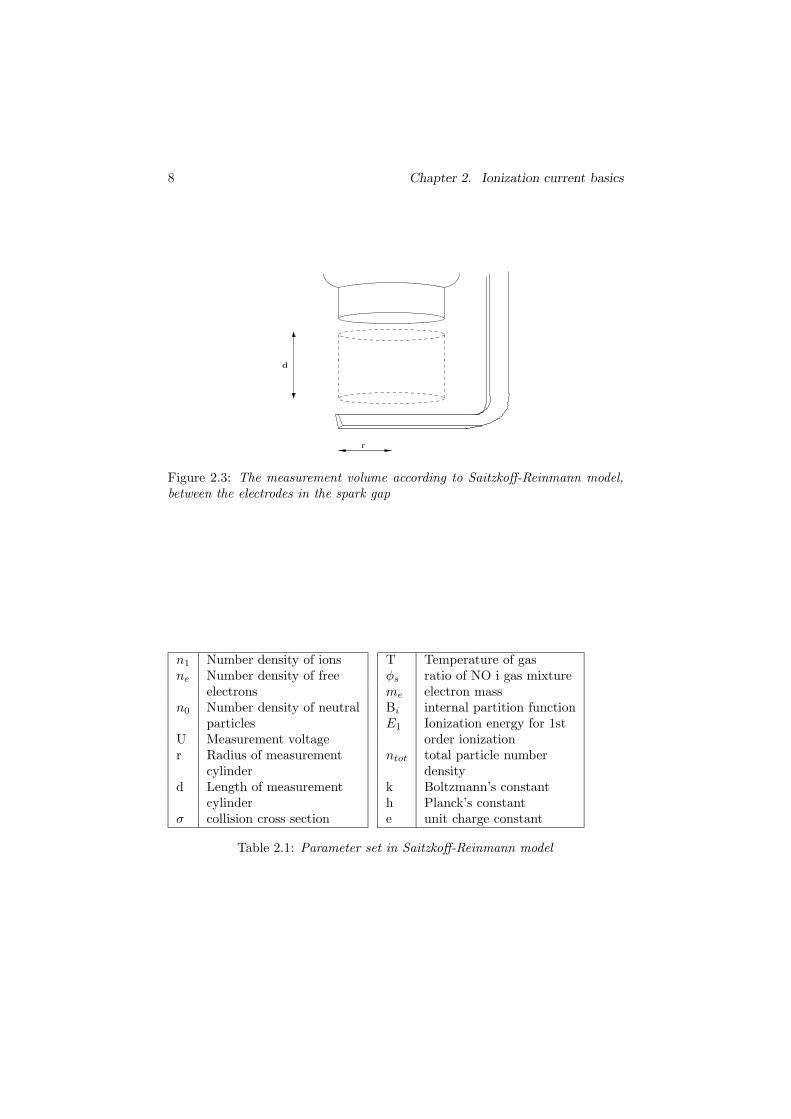
2.2.1 Saitzkoff-Reinmann model
A model for the second peak of the ion current was presented by Saitzkoffet al. (1996). Figure 2.3 shows the idea behind the model. A cylinder shapedcontrol volume between the two spark plug electrodes contains free electronsfrom thermal ionization of NO. The electrical field between the electrodes createa movement of the electrons. The movement of free electrons dominates thecurrent since they are highly mobile compared to positive ions. The dominatingprocess for generating free electrons is the thermal ionization of NO and can bedescribed by Saha’s equation (see Saitzkoff et al. (1996) for assumptions)
n1ne
n0= 2
(
2πmekT
h2
)32 B1
B0exp
[
−E1
kT
]
(2.1)
which describes the equilibrium balance of ions and electrons for a first orderionization. When combined with models for electron drift velocity and electricfield an expression for ion current is obtained as (Saitzkoff et al., 1996)
I = Uπr2
d
e2
σme
√
8kTπme
√
φs
√
√
√
√2(
2πmekTh2
)32 B1
B0exp
[
−E1
kT
]
ntot(2.2)
Table 2.1 describes all entries in Equations (2.1) and (2.2).
8 Chapter 2. Ionization current basics
r
d
Figure 2.3: The measurement volume according to Saitzkoff-Reinmann model,between the electrodes in the spark gap
n1 Number density of ionsne Number density of free
electronsn0 Number density of neutral
particlesU Measurement voltager Radius of measurement
cylinderd Length of measurement
cylinderσ collision cross section
T Temperature of gasφs ratio of NO i gas mixtureme electron massBi internal partition functionE1 Ionization energy for 1st
order ionizationntot total particle number
densityk Boltzmann’s constanth Planck’s constante unit charge constant
Table 2.1: Parameter set in Saitzkoff-Reinmann model
2.2. Existing models 9
The model sees a free space charge that is affected by the electrical fieldgenerated by the measurement probe, the spark plug. The movement of thecharge does not change the field inside the combustion chamber significantlysince the re-distributed charge is at such a low magnitude. The movement ishowever measurable in the outer circuit. The main limit for the current is theaccess of free electrons. This is the main difference compared to other models.
Wilstermann (1999) presented a similar model. The model uses more de-tailed calculations on electric field and has added chemical reactions in the flamefront as a source for free charge.
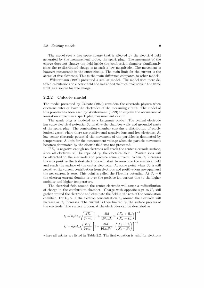
2.2.2 Calcote model
The model presented by Calcote (1963) considers the electrode physics whenelectrons enter or leave the electrodes of the measuring circuit. The model ofthis process has been used by Wilstermann (1999) to explain the occurrence ofionization current in a spark plug measurement circuit.
The spark plug is modeled as a Langmuir probe. The central electrodehas some electrical potential Us relative the chamber walls and grounded partsof the spark plug. The combustion chamber contains a distribution of partlyionized gases, where there are positive and negative ions and free electrons. Atlow center electrode potential the movement of the particles is dominated bytemperature. A limit for the measurement voltage when the particle movementbecomes dominated by the electric field was not presented.
If Us is negative enough no electrons will reach the center electrode surface,since all electrons will be repelled by the electrical field. Positive ions willbe attracted to the electrode and produce some current. When Us increasestowards positive the fastest electrons will start to overcome the electrical fieldand reach the surface of the center electrode. At some point when Us is stillnegative, the current contribution from electrons and positive ions are equal andthe net current is zero. This point is called the Floating potential. At Us = 0the electron current dominates over the positive ion current due to the highermobility and higher temperature.
The electrical field around the center electrode will cause a redistributionof charge in the combustion chamber. Charge with opposite sign to Us willgather around the electrode and eliminate the field in the rest of the combustionchamber. For Us > 0, the electron concentration ne around the electrode willincrease as Us increases. The current is then limited by the surface process ofthe electrode. The surface process at the electrodes can be described as
Ie = neeAs
√
kTe
2πme
[
1 +3ld
16λeBeln
(
Xe + Be
Xe − Be
)]
−1
Ii = nieAs
√
kTi
2πmi
[
1 +3ld
16λiBiln
(
Xi + Bi
Xi − Bi
)]
−1
where all entries are listed in Table 2.2. The first equation is valid for electrons
10 Chapter 2. Ionization current basics
ne electron concentrationme electron massTe Electron temperatureλe electron mean free pathe unit chargel probe lengthd probe diameterAs probe surface area
Xe = l + 2λe
Be =√
X2e − (d + 2λe)2
ni ion concentrationmi ion massTi ion temperatureλi ion mean free pathXi = l + 2λi
Bi =√
X2i − (d + 2λi)2
Table 2.2: Parameter set in Calcote model
at a positive electrode and the second is valid for positive ions at a negativeelectrode.
Typically, ion current measurement systems of today use a positive centerelectrode potential. The electron current at the positive electrode dominatesthe total current due to the lower mass and higher temperature of the electronscompared to the ions. As the measurement voltage Us increases, the electronconcentration around the electrode ne increases and therefore the current. Theassumption here is that the access of free electrons in the combustion chamberis sufficient for the needed redistribution. No equation for the relation betweenne and Us was given.
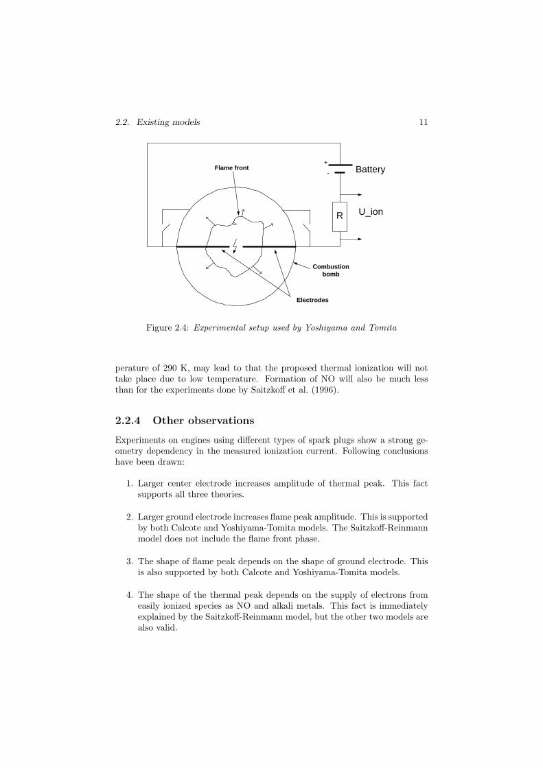
2.2.3 Yoshiyama-Tomita model
Yoshiyama et al. (2000) presented a theory based on flame front ionization.Experiments were made in a combustion bomb as in Figure 2.4. The combus-tion bomb has a spark gap between two electrodes which are isolated exceptfor the top where the spark is fired. The bomb wall can be electrically isolatedor connected to one of the electrodes. An air-fuel mixture was ignited and theionization current was measured between the electrodes for different electricalconfigurations of the chamber wall. A camera was monitoring the flame prop-agation and the pictures were synchronized with the measured current. Theresulting current shows the two characteristic peaks, in some cases. The firstion peak appears when the flame front is close to the spark gap in all tests. Thesecond peak appears only for the case when the wall is connected to the negativeelectrode and when the flame front reaches the wall. From the experiments twoconclusions were drawn:
• The ionization current shape is dependent of flame position and electrodepolarity.
• Ions and electrons are generated in the flame front by chemical reactionsand thermal ionization is negligible.
The presented theory explains the results from the experiments made. How-ever, the conditions in the experiments, start pressure of 4 bar and start tem-
2.2. Existing models 11
+
-
R U_ion
Battery
Combustion bomb
Electrodes
Flame front
Figure 2.4: Experimental setup used by Yoshiyama and Tomita
perature of 290 K, may lead to that the proposed thermal ionization will nottake place due to low temperature. Formation of NO will also be much lessthan for the experiments done by Saitzkoff et al. (1996).
2.2.4 Other observations
Experiments on engines using different types of spark plugs show a strong ge-ometry dependency in the measured ionization current. Following conclusionshave been drawn:
1. Larger center electrode increases amplitude of thermal peak. This factsupports all three theories.
2. Larger ground electrode increases flame peak amplitude. This is supportedby both Calcote and Yoshiyama-Tomita models. The Saitzkoff-Reinmannmodel does not include the flame front phase.
3. The shape of flame peak depends on the shape of ground electrode. Thisis also supported by both Calcote and Yoshiyama-Tomita models.
4. The shape of the thermal peak depends on the supply of electrons fromeasily ionized species as NO and alkali metals. This fact is immediatelyexplained by the Saitzkoff-Reinmann model, but the other two models arealso valid.
12 Chapter 2. Ionization current basics
+ -
-
+
Ion meas. R
Combustionchamber
+
-
+
-
1
3
2
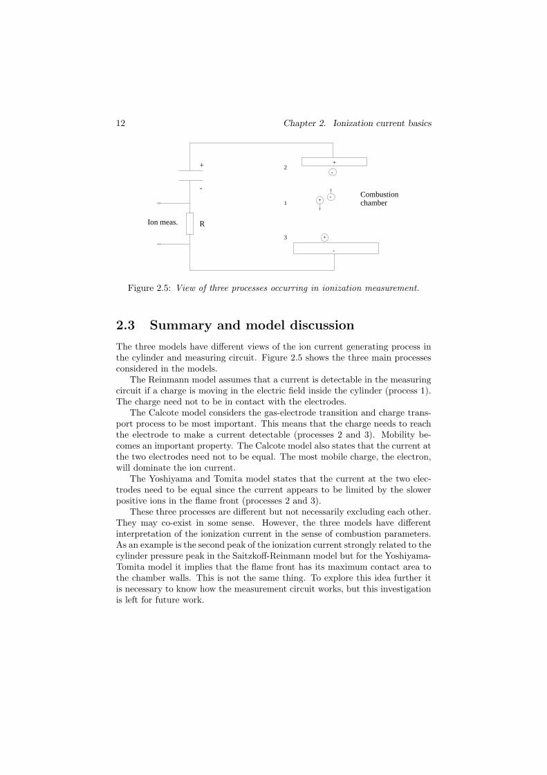
Figure 2.5: View of three processes occurring in ionization measurement.
2.3 Summary and model discussion
The three models have different views of the ion current generating process inthe cylinder and measuring circuit. Figure 2.5 shows the three main processesconsidered in the models.
The Reinmann model assumes that a current is detectable in the measuringcircuit if a charge is moving in the electric field inside the cylinder (process 1).The charge need not to be in contact with the electrodes.
The Calcote model considers the gas-electrode transition and charge trans-port process to be most important. This means that the charge needs to reachthe electrode to make a current detectable (processes 2 and 3). Mobility be-comes an important property. The Calcote model also states that the current atthe two electrodes need not to be equal. The most mobile charge, the electron,will dominate the ion current.
The Yoshiyama and Tomita model states that the current at the two elec-trodes need to be equal since the current appears to be limited by the slowerpositive ions in the flame front (processes 2 and 3).
These three processes are different but not necessarily excluding each other.They may co-exist in some sense. However, the three models have differentinterpretation of the ionization current in the sense of combustion parameters.As an example is the second peak of the ionization current strongly related to thecylinder pressure peak in the Saitzkoff-Reinmann model but for the Yoshiyama-Tomita model it implies that the flame front has its maximum contact area tothe chamber walls. This is not the same thing. To explore this idea further itis necessary to know how the measurement circuit works, but this investigationis left for future work.
3
NO formation and thermal
ionization
This section presents an analysis of the ionization current model suggested bySaitzkoff and Reinmann in more detail. The base is thermal ionization of nitricoxide, NO. The model is built up by two processes, NO formation and ther-mal ionization, with combustion temperature and air-fuel ratio as inputs. Thetwo processes are summarized here and finally the temperature sensitivity isdiscussed.
The composition of the burned gases is changed during the progress of a com-bustion. The formation of major exhaust gas components have been describedwith chemical reactions, balanced by temperature dependent equilibrium con-stants by Lavoie et al. (1970) and Heywood (1988). Most reactions, except forNO formation, are described as fast compared to the time-scale of a combustionand concentrations are close to equilibrium. The formation of NO is slower andis better described as reaction rate limited rather than in equilibrium. Twoquestions are addressed here:
1. Is NO the most probable main contributor of free charge from thermalionization?
2. What impact does combustion temperature and NO content have on ion-ization current amplitude?
3.1 NO formation theory
Heywood (1988) gave a description of the process behind NO formation, basedon the Zeldowich mechanism (Zeldovich et al., 1947). This is a summary of
13
14 Chapter 3. NO formation and thermal ionization
the processes described by Heywood and this model is referred to as the dy-namic NO formation or reaction rate controlled NO formation in this thesis.The description by Heywood (1988) does not cover formation of all species inthe reactions. Concentrations of different species, needed as inputs, were calcu-lated by the Matlab program package CHEPP (Eriksson, 2000). To validate theimplementation of the dynamic NO formation model, the calculation of equi-librium concentration of NO is compared between the Heywood model and theCHEPP tool. Also Figure 11.7 in (Heywood, 1988) was produced as a recieptthat the implementation was equal to the one by Heywood.
The extended Zeldovich mechanism (Zeldovich et al., 1947; Lavoie et al.,1970) lists the dominating reactions for forming NO:
O + N2 NO + N
N + O2 NO + O
N + OH NO + H
Two assumptions are made:
1. the content of N is small and changes slowly compared to the content ofNO
2. concentrations of O, O2, OH, H and N2 can be approximated by theirequilibrium concentrations
With these assumptions the following expression for NO formation is derived:
d [NO]
dt=
2R1(1 − ([NO]/[NO]e)2)
1 + ([NO]/[NO]e)R1/(R2 + R3)(3.1)
where
R1 = k+1 [O]e[N2]e = k−
1 [NO]e[N ]e
R2 = k+2 [N ]e[O2]e = k−
2 [NO]e[O]e
R3 = k+3 [N ]e[OH]e = k−
3 [NO]e[H]e
The concentration [ ] is in the unit [mol/cm3] and the reaction rate constantsare listed in Table 3.1 (Heywood, 1988). The concentration [NO] is defined as
[NO] =NNO
V(3.2)
where NNO is the quantity of NO in [mol] distributed in the volume V. For aconstant volume V Equation (3.1) can equivalently be written as
1
V
dNNO
dt=
2R1(1 − ([NO]/[NO]e)2)
1 + ([NO]/[NO]e)R1/(R2 + R3)(3.3)
3.1. NO formation theory 15
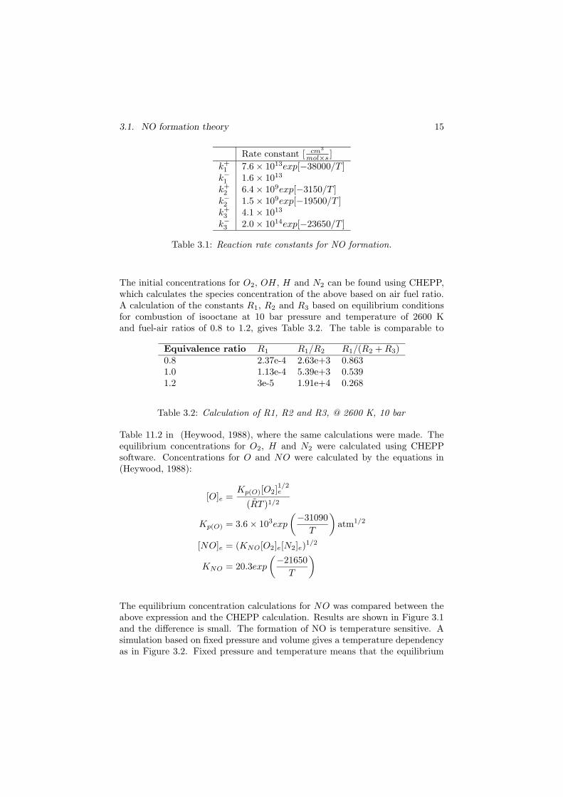
Rate constant [ cm3
mol×s ]
k+1 7.6 × 10¹³exp[−38000/T ]
k−
1 1.6 × 10¹³
k+2 6.4 × 10⁹exp[−3150/T ]
k−
2 1.5 × 10⁹exp[−19500/T ]k+3 4.1 × 10¹³
k−
3 2.0 × 10¹⁴exp[−23650/T ]
Table 3.1: Reaction rate constants for NO formation.
The initial concentrations for O2, OH, H and N2 can be found using CHEPP,which calculates the species concentration of the above based on air fuel ratio.A calculation of the constants R1, R2 and R3 based on equilibrium conditionsfor combustion of isooctane at 10 bar pressure and temperature of 2600 Kand fuel-air ratios of 0.8 to 1.2, gives Table 3.2. The table is comparable to
Equivalence ratio R1 R1/R2 R1/(R2 + R3)0.8 2.37e-4 2.63e+3 0.8631.0 1.13e-4 5.39e+3 0.5391.2 3e-5 1.91e+4 0.268
Table 3.2: Calculation of R1, R2 and R3, @ 2600 K, 10 bar
Table 11.2 in (Heywood, 1988), where the same calculations were made. Theequilibrium concentrations for O2, H and N2 were calculated using CHEPPsoftware. Concentrations for O and NO were calculated by the equations in(Heywood, 1988):
[O]e =Kp(O)[O2]
1/2e
(RT )1/2
Kp(O) = 3.6 × 10³exp
(
−31090
T
)
atm1/2
[NO]e = (KNO[O2]e[N2]e)1/2
KNO = 20.3exp
(
−21650
T
)
The equilibrium concentration calculations for NO was compared between theabove expression and the CHEPP calculation. Results are shown in Figure 3.1and the difference is small. The formation of NO is temperature sensitive. Asimulation based on fixed pressure and volume gives a temperature dependencyas in Figure 3.2. Fixed pressure and temperature means that the equilibrium
16 Chapter 3. NO formation and thermal ionization
−60 −40 −20 0 20 40 60 800
1
2
3
4
5
6x 10
−7
Chepp
Heywood
sim
xN
Oe
CAD
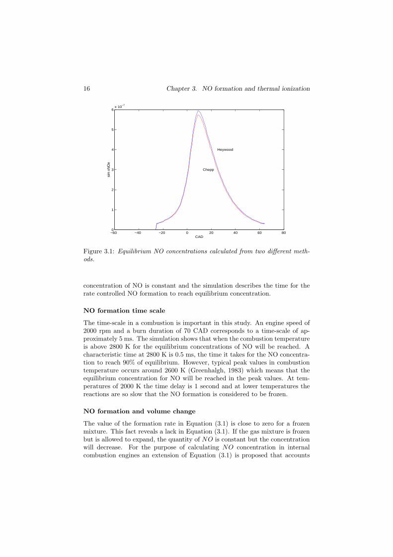
Figure 3.1: Equilibrium NO concentrations calculated from two different meth-ods.
concentration of NO is constant and the simulation describes the time for therate controlled NO formation to reach equilibrium concentration.
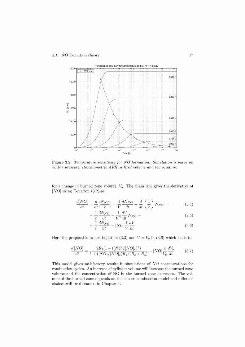
NO formation time scale
The time-scale in a combustion is important in this study. An engine speed of2000 rpm and a burn duration of 70 CAD corresponds to a time-scale of ap-proximately 5 ms. The simulation shows that when the combustion temperatureis above 2800 K for the equilibrium concentrations of NO will be reached. Acharacteristic time at 2800 K is 0.5 ms, the time it takes for the NO concentra-tion to reach 90% of equilibrium. However, typical peak values in combustiontemperature occurs around 2600 K (Greenhalgh, 1983) which means that theequilibrium concentration for NO will be reached in the peak values. At tem-peratures of 2000 K the time delay is 1 second and at lower temperatures thereactions are so slow that the NO formation is considered to be frozen.
NO formation and volume change
The value of the formation rate in Equation (3.1) is close to zero for a frozenmixture. This fact reveals a lack in Equation (3.1). If the gas mixture is frozenbut is allowed to expand, the quantity of NO is constant but the concentrationwill decrease. For the purpose of calculating NO concentration in internalcombustion engines an extension of Equation (3.1) is proposed that accounts
3.1. NO formation theory 17
10−6
10−5
10−4
10−3
10−2
10−1
100
101
0
2000
4000
6000
8000
10000
12000Temperature sensitivity for NO formation, 50 bar, AFR = stoich.
NO
[ppm
]
Time [s]
2000 K
2200 K
2400 K
2600 K
2800 K
3000 K
90% time
Figure 3.2: Temperature sensitivity for NO formation. Simulation is based on50 bar pressure, stoichiometric AFR, a fixed volume and temperature.
for a change in burned zone volume, Vb. The chain rule gives the derivative of[NO] using Equation (3.2) as:
d[NO]
dt=
d
dt(NNO
V) =
1
V
dNNO
dt+
d
dt
(
1
V
)
NNO = (3.4)
=1
V
dNNO
dt−
1
V 2
dV
dtNNO = (3.5)
=1
V
dNNO
dt− [NO]
1
V
dV
dt(3.6)
Here the proposal is to use Equation (3.3) and V = Vb in (3.6) which leads to
d [NO]
dt=
2R1(1 − ([NO]/[NO]e)2)
1 + ([NO]/[NO]e)R1/(R2 + R3)− [NO]
1
Vb
dVb
dt(3.7)
This model gives satisfactory results in simulations of NO concentrations forcombustion cycles. An increase of cylinder volume will increase the burned zonevolume and the concentration of NO in the burned zone decreases. The vol-ume of the burned zone depends on the chosen combustion model and differentchoices will be discussed in Chapter 4.
18 Chapter 3. NO formation and thermal ionization
−40 −20 0 20 40 60 80 100 1200
20
40
60C
yl p
[bar
]
NO formation in burned zone, two−zone model
−40 −20 0 20 40 60 80 100 1200
1000
2000
3000
4000
Cyl
tem
p [K
]
Tb
Tu
−40 −20 0 20 40 60 80 100 1200
5000
10000
15000
NO
[ppm
]
Reaction rate contr. NO
Equilibrium contr. NO
Figure 3.3: NO formation simulated from engine pressure data
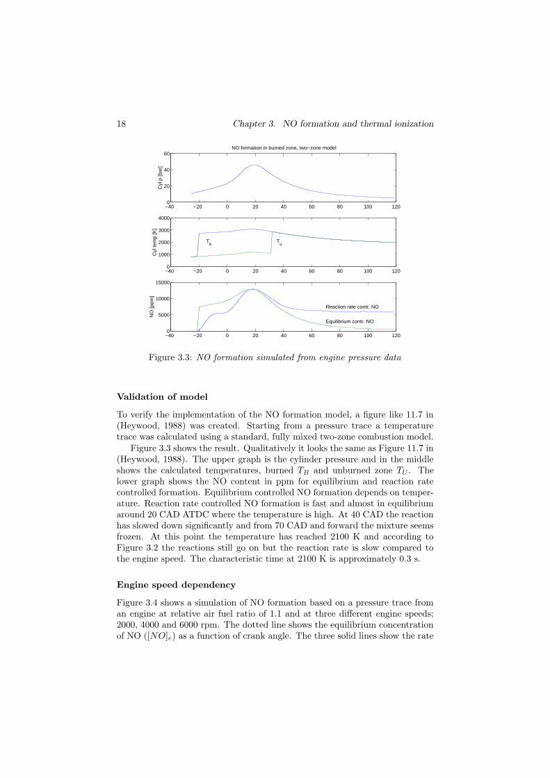
Validation of model
To verify the implementation of the NO formation model, a figure like 11.7 in(Heywood, 1988) was created. Starting from a pressure trace a temperaturetrace was calculated using a standard, fully mixed two-zone combustion model.
Figure 3.3 shows the result. Qualitatively it looks the same as Figure 11.7 in(Heywood, 1988). The upper graph is the cylinder pressure and in the middleshows the calculated temperatures, burned TB and unburned zone TU . Thelower graph shows the NO content in ppm for equilibrium and reaction ratecontrolled formation. Equilibrium controlled NO formation depends on temper-ature. Reaction rate controlled NO formation is fast and almost in equilibriumaround 20 CAD ATDC where the temperature is high. At 40 CAD the reactionhas slowed down significantly and from 70 CAD and forward the mixture seemsfrozen. At this point the temperature has reached 2100 K and according toFigure 3.2 the reactions still go on but the reaction rate is slow compared tothe engine speed. The characteristic time at 2100 K is approximately 0.3 s.
Engine speed dependency
Figure 3.4 shows a simulation of NO formation based on a pressure trace froman engine at relative air fuel ratio of 1.1 and at three different engine speeds;2000, 4000 and 6000 rpm. The dotted line shows the equilibrium concentrationof NO ([NO]e) as a function of crank angle. The three solid lines show the rate

3.2. Thermal ionization theory 19
−100 −50 0 50 100 150 2000
0.5
1
1.5
2
2.5
3
3.5x 10
−6
Time [CAD]
xNO
[mol
/cm
3]
NO formation simulated at 1.0 bar intake pressure
−100 −50 0 50 100 150 2000
1000
2000
3000
4000
Time [CAD]
Bur
ned
gas
tem
p [K
]Burned gas temperature at 1.0 bar intake pressure
Figure 3.4: Reaction rate controlled NO formation compared to equilibrium con-trolled at different engine speeds; 2000, 4000 and 6000 rpm.
controlled NO concentration ([NO]). The slowest combustion happens for thelowest engine speed and [NO] for this case falls closest to [NO]e.
The difference in [NO] for different engine speeds appear when the com-bustion temperature passes through the region where the characteristic timeof NO reactions is in the same order as the time-scale of the combustion. Forhigher engine speed the temperature will spend less time in this region and[NO] deviates from [NO]e.
3.2 Thermal ionization theory
A detailed description of thermal ionization process was given by Saitzkoff et al.(1996) in appendix A. The balance between generation and regeneration of ionscaused by thermal excitation forms the basis for the ionization. The ionizationprocess is assumed to be fast compared to the combustion process and specif-ically the combustion temperature development. Therefore the electrons andions are in thermodynamic equilibrium and the balance can be described by theSaha equation
nine
ni−1= 2
(
2πmekT
h2
)32 Bi
Bi−1exp
[
−Ei
kT
]
(3.8)
20 Chapter 3. NO formation and thermal ionization
n is number density for species of ionized state i, i-1 and electrons e. me is theelectron mass, k is Boltzmann’s constant, h Planck’s constant, Ei ionizationenergy for ionized state i, T is the mixture temperature and B is the internalpartition function. Saitzkoff et al. (1996) assumed that NO is only ionized tothe first level. If the ionization ratio is defined as
η =ne
n0 + ni(3.9)
and assuming only first level ionization
ne = ni = n1 (3.10)
Combining expressions (3.8), (3.9) and (3.10) gives an expression for ionizationratio η
η =
√
nH
n0
nH = 2
(
2πmekT
h2
)32 B1
B0exp
[
−Ei
kT
]
where n0 is the number density of the neutral species.Using the CHEPP software for equilibrium concentration calculations of
burned gas species, some other sources for thermal ionization may be explored.The ionization energy for different species are listed in Table 3.3. The impact
Species Ionization energy (eV)H 13,6H2 15,4O 13,6O2 12,1OH 13,2H2O 12,6CO 14,0CO2 13,8NO 9,2N2 15,6
Table 3.3: Ionization energies for dominant combustion species, from Wilster-mann (1999)
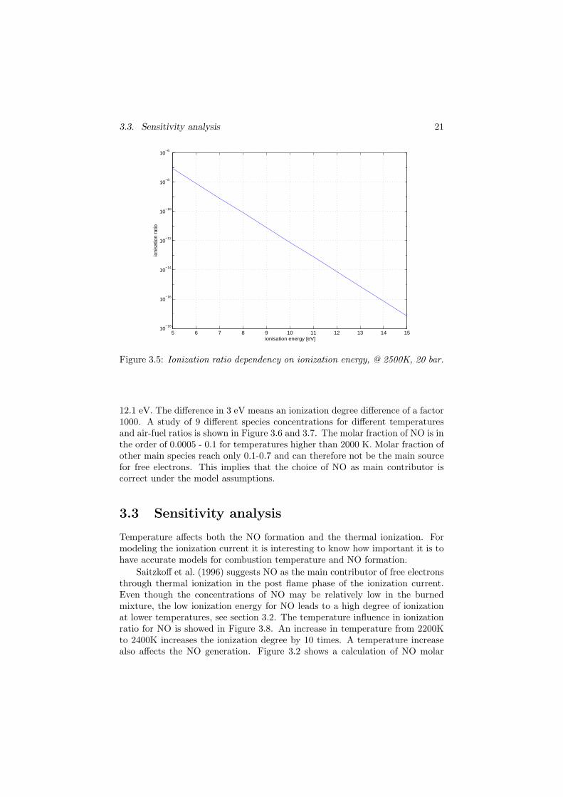
of ionization energy is seen in Figure 3.5. An increase of 1 eV in ionizationenergy will decrease the ionization ratio with a factor of 10. One other specieswith higher ionization energy than NO has to have a correspondingly higherconcentration to produce the same amount of ions. Considering Table 3.3 itis seen that from the listed species the closest in ionization energy is O2 with
3.3. Sensitivity analysis 21
5 6 7 8 9 10 11 12 13 14 1510
−18
10−16
10−14
10−12
10−10
10−8
10−6
ioni
satio
n ra
tio
ionisation energy [eV]
Figure 3.5: Ionization ratio dependency on ionization energy, @ 2500K, 20 bar.
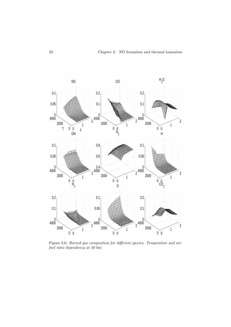
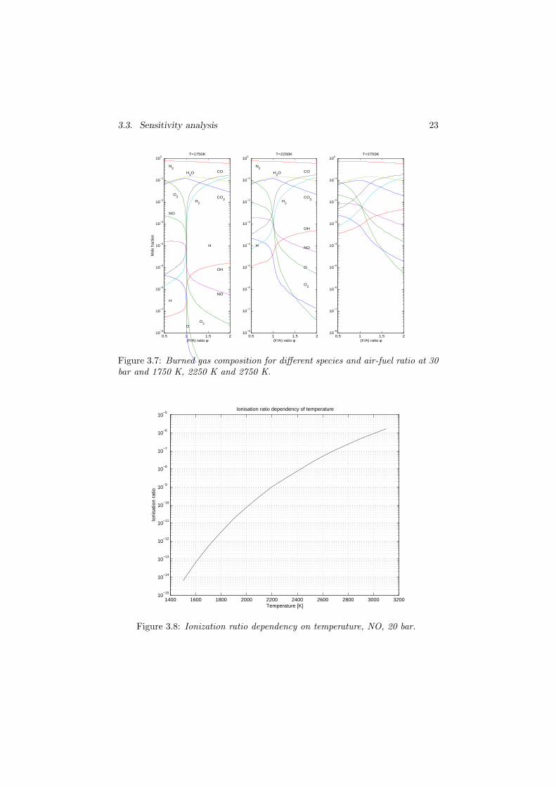
12.1 eV. The difference in 3 eV means an ionization degree difference of a factor1000. A study of 9 different species concentrations for different temperaturesand air-fuel ratios is shown in Figure 3.6 and 3.7. The molar fraction of NO is inthe order of 0.0005 - 0.1 for temperatures higher than 2000 K. Molar fraction ofother main species reach only 0.1-0.7 and can therefore not be the main sourcefor free electrons. This implies that the choice of NO as main contributor iscorrect under the model assumptions.
3.3 Sensitivity analysis
Temperature affects both the NO formation and the thermal ionization. Formodeling the ionization current it is interesting to know how important it is tohave accurate models for combustion temperature and NO formation.
Saitzkoff et al. (1996) suggests NO as the main contributor of free electronsthrough thermal ionization in the post flame phase of the ionization current.Even though the concentrations of NO may be relatively low in the burnedmixture, the low ionization energy for NO leads to a high degree of ionizationat lower temperatures, see section 3.2. The temperature influence in ionizationratio for NO is showed in Figure 3.8. An increase in temperature from 2200Kto 2400K increases the ionization degree by 10 times. A temperature increasealso affects the NO generation. Figure 3.2 shows a calculation of NO molar
22 Chapter 3. NO formation and thermal ionization
01
2
02000
40000
0.05
0.1
λ
NO
T 01
2
02000
40000
0.1
0.2
CO
01
2
02000
40000
0.1
0.2
H2O
01
2
02000
40000
0.05
0.1
OH
01
2
02000
40000.4
0.6
0.8
N2
01
2
02000
40000
0.05
0.1
H
01
2
02000
40000
0.1
0.2
H2
01
2
02000
40000
0.05
0.1
O
01
2
02000
40000
0.1
0.2
CO2
Figure 3.6: Burned gas composition for different species. Temperature and air-fuel ratio dependency at 20 bar.
3.3. Sensitivity analysis 23
0.5 1 1.5 210
−8
10−7
10−6
10−5
10−4
10−3
10−2
10−1
100
T=1750K
(F/A) ratio φ
Mol
e fra
ctio
n
N2
CO2
H2O CO
H2
H
OH
O2
O2
NO
NO
H
O
0.5 1 1.5 210
−8
10−7
10−6
10−5
10−4
10−3
10−2
10−1
100
(F/A) ratio φ
T=2250K
N2
CO2
H2O CO
H2
NO
OH
H
O
O2
0.5 1 1.5 210
−8
10−7
10−6
10−5
10−4
10−3
10−2
10−1
100
(F/A) ratio φ
T=2750K
Figure 3.7: Burned gas composition for different species and air-fuel ratio at 30bar and 1750 K, 2250 K and 2750 K.
1400 1600 1800 2000 2200 2400 2600 2800 3000 320010
−15
10−14
10−13
10−12
10−11
10−10
10−9
10−8
10−7
10−6
10−5
Ioni
satio
n ra
tio
Temperature [K]
Ionisation ratio dependency of temperature
Figure 3.8: Ionization ratio dependency on temperature, NO, 20 bar.
24 Chapter 3. NO formation and thermal ionization
fraction development for different fix temperatures. The end value correspondsto equilibrium conditions. The equilibrium fraction for NO increases 2 timeswhen temperature rises from 2200K to 2400K. However, in a combustion thetemperature only stays at the peak level in the order of milliseconds.
Reaction rate limited NO formation is most important for temperatureswhere the reactions are slow compared to the combustion event, below 2600 Kwhere the characteristic time is 3 ms. For temperatures above 2600 K thereactions are fast and the NO concentration reaches equilibrium. In the range2600 - 3000 K the NO fraction increases 3 times and the ionization degree 20times. If the combustion temperature reaches this region the ionization degreedominates over the NO formation. Using a fix level of NO fraction introduces arelatively small error in amplitude. At 1 ms the increase in NO molar fractionis 18 times.
The same analysis for a temperature step from 2400 K to 2600 K gives 10times ionization degree increase and 2 times NO molar fraction increase at 1 ms.Table 3.4 views how a temperature change impacts on the ionization current.
Temp step Ionization degree NO molar fraction Total ion curr.2200K - 2400K ×10 ×18 422400K - 2600K ×10 ×2 14
Table 3.4: Impact of temperature change in ionization current
First column is the temperature step, the second is the increase in ionizationdegree, the third is the increase in NO molar fraction at 1 ms and the fourthcolumn is the total increase in ionization current according to the Saitzkoffmodel. The ionization current model in Equation (2.2) can be simplified to
I = A√
φNO exp
[
−ENO
2kT
]
(3.11)
where I is the current, φNO is the molar fraction of NO in the combustedgas, the exponential factor represents the temperature sensitive part of theionization degree and A gathers all parts of Equation (2.2) that is not affectedby temperature. Actually, one factor in A is T 1/4 but its impact on I when Tchanges is negligible compared to the exponential factor.
The ionization current sensitivity differs between the two sources NO molarfraction and ionization degree. The ionization degree comes in linearly butthe NO molar fraction comes in as the square root. Both are dependent oftemperature and while the ionization degree obviously relates exponentiallyto the temperature, the NO content relation is not easily unmasked and isinvestigated with a simple numerical approach instead. The relative gradientsof NO content and ionization degree with respect to temperature give a measurefor the sensitivity.
3.4. Conclusions 25
10−5
10−4
10−3
10−2
10−1
100
101
1800
2000
2200
2400
2600
2800
3000T
empe
ratu
re [K
]
NO characteristic time 90% [s]
1800 2000 2200 2400 2600 2800 30000
2
4
6
8
Temperature [K]
Rel
ativ
e gr
adie
nt [%
/K]
NO @ 1 ms Ionisation
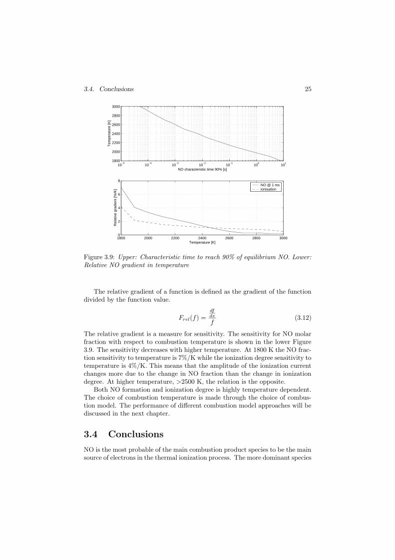
Figure 3.9: Upper: Characteristic time to reach 90% of equilibrium NO. Lower:Relative NO gradient in temperature
The relative gradient of a function is defined as the gradient of the functiondivided by the function value.
Frel(f) =dfdx
f(3.12)
The relative gradient is a measure for sensitivity. The sensitivity for NO molarfraction with respect to combustion temperature is shown in the lower Figure3.9. The sensitivity decreases with higher temperature. At 1800 K the NO frac-tion sensitivity to temperature is 7%/K while the ionization degree sensitivity totemperature is 4%/K. This means that the amplitude of the ionization currentchanges more due to the change in NO fraction than the change in ionizationdegree. At higher temperature, >2500 K, the relation is the opposite.
Both NO formation and ionization degree is highly temperature dependent.The choice of combustion temperature is made through the choice of combus-tion model. The performance of different combustion model approaches will bediscussed in the next chapter.
3.4 Conclusions
NO is the most probable of the main combustion product species to be the mainsource of electrons in the thermal ionization process. The more dominant species
26 Chapter 3. NO formation and thermal ionization
in the combusted gas, CO2, H2O and N2, all have so much higher ionizationenergy that the total number of ionized particles from these three is much lessthan from NO. Also, NO has least ionization energy of all species with equal orless concentration than NO.
An extension to the NO formation model presented by Heywood (1988) wasdeveloped, that considers the volume change in the burned zone and makes theNO formation model useful in engine cycle calculation.
According to the model presented by Saitzkoff et al. (1996) the amplitude ofthe ionization current is affected by both NO content and thermal ionization.In the higher temperature region, >2400 K, thermal ionization dominates insensitivity. In the lower region, <2400 K, the NO formation processes is moreimportant.
4
Temperature models for
ionization current description
A combustion model can describe the temperature development in the cylinder.Combustion models may be classified in dimensions and zones. A single-zonemodel considers the whole combustion chamber to be one zone. A two-zonemodel divides the combustion chamber in two zones where each zone have itsown temperature, volume and mass but share pressure. A zero-dimensionalmodel has no variations in chemical composition, temperature or pressure withineach zone. All investigated models in this chapter are zero-dimensional. Amultidimensional model is based on fluid dynamics that give information onthe flow field in the combustion chamber. This feature can be useful if flamedevelopment is modeled. In this case flame development is given via the heatrelease rate that comes from analysis of pressure data.
The purpose of this chapter is to find a combustion model that describesthe combustion temperature in a way that it explains the ionization current.The three different model approaches taken in this chapter are two extremesand one compromise. The two extremes represent the lowest (one-zone) and thehighest (kernel zone) possible combustion temperatures from a thermodynamicperspective and the compromise (two-zone) a temperature in between the twoextremes. Also, an interesting question is whether a dynamic NO formationmodel has any impact on the ionization current. Earlier work by Saitzkoff et al.(1996) used a fix NO molar fraction of 1%. This level is supported by the workof Lavoie et al. (1970). The first model upgrade would be to use equilibriumconcentrations of NO based on combustion pressure and temperature, and gascomposition. However, a reaction rate controlled NO formation process has aproperty that effects both timing and amplitude of the NO content which may
27
28 Chapter 4. Temperature models for ionization current description
be useful in the medium temperature area 1800 K to 2400 K. Therefore theequilibrium model step was excluded and the effort was put to investigate thereaction rate controlled NO formation process.
In this case cylinder pressure and cylinder volume are the inputs to themodel. The outputs from the model are a combustion temperature trace andthe volume of the burned zone. In the case of the one-zone model, the wholecylinder volume is the burned zone.
4.1 One-zone model
A one-zone combustion model considers the whole combustion chamber as onezone and the gas mixture is an ideal gas. This one-zone model represents thelowest possible combustion temperature since the energy released from combus-tion warms up the whole mixture. The combustion zone volume is equal to thecylinder volume. The gas mass is constant during the whole combustion sinceblow-by is neglected. The gas constant R can have different level of accuracy.It is calculated as
R =R
M
where R = 8, 31[J/molK] is the universal gas constant and M is the meanmolecular weight of the gas mixture. In this case M is a constant. In the casewhere the cylinder pressure, volume and mass is known, the cylinder tempera-ture is easily derived by the ideal gas law
T =p V
mR(4.1)
4.2 Kernel zone model
The highest possible combustion temperature can be reached when the com-busted gas is not mixed with any cooler gas. The warmest gas appears in thebeginning of combustion if it is allowed to be compressed without heat transferto the surroundings. The kernel zone model is described as follows.
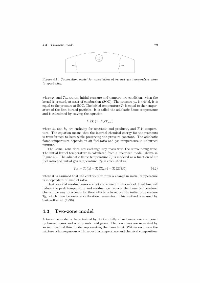
A small kernel of burned gas is located at the spark plug, as in Figure 4.1.Two assumptions are made about the gas kernel:
1. Burned gas mixing is negligible
2. Heat loss to the surrounding environment is negligible
The kernel of gas is compressed and expanded adiabatically by the surroundingcylinder pressure according to
(
p
p0
)γ−1
γ
=Tk
Tk0
4.3. Two-zone model 29
Tkntot
Figure 4.1: Combustion model for calculation of burned gas temperature closeto spark plug.
where p0 and Tk0 are the initial pressure and temperature conditions when thekernel is created, at start of combustion (SOC). The pressure p0 is trivial, it isequal to the pressure at SOC. The initial temperature T0 is equal to the temper-ature of the first burned particles. It is called the adiabatic flame temperatureand is calculated by solving the equation:
hr(Tr) = hp(Tp, p)
where hr and hp are enthalpy for reactants and products, and T is tempera-ture. The equation means that the internal chemical energy for the reactantsis transformed to heat while preserving the pressure constant. The adiabaticflame temperature depends on air-fuel ratio and gas temperature in unburnedmixture.
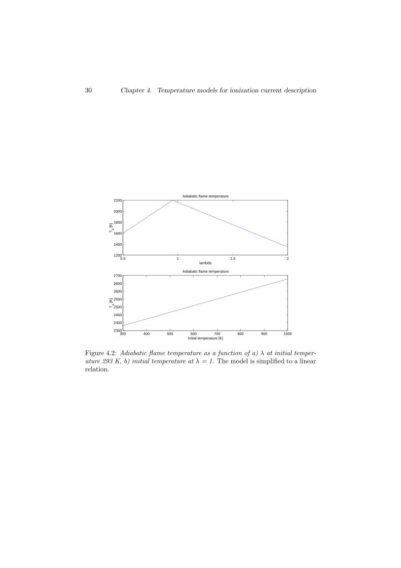
The kernel zone does not exchange any mass with the surrounding zone.The initial kernel temperature is calculated from a linearized model, shown inFigure 4.2. The adiabatic flame temperature T0 is modeled as a function of airfuel ratio and initial gas temperature. T0 is calculated as
Tk0 = Ta(λ) + Ta(Tinit) − Ta(293K) (4.2)
where it is assumed that the contribution from a change in initial temperatureis independent of air-fuel ratio.
Heat loss and residual gases are not considered in this model. Heat loss willreduce the peak temperature and residual gas reduces the flame temperature.One simple way to account for these effects is to reduce the initial temperatureT0, which then becomes a calibration parameter. This method was used bySaitzkoff et al. (1996).
4.3 Two-zone model
A two-zone model is characterized by the two, fully mixed zones, one composedby burned gases and one by unburned gases. The two zones are separated byan infinitesimal thin divider representing the flame front. Within each zone themixture is homogeneous with respect to temperature and chemical composition.
30 Chapter 4. Temperature models for ionization current description
0.5 1 1.5 21200
1400
1600
1800
2000
2200
Ta [K
]
Adiabatic flame temperature
lambda
300 400 500 600 700 800 900 10002350
2400
2450
2500
2550
2600
2650
2700
Ta [K
]
Adiabatic flame temperature
Initial temperature [K]
Figure 4.2: Adiabatic flame temperature as a function of a) λ at initial temper-ature 293 K, b) initial temperature at λ = 1. The model is simplified to a linearrelation.
4.3. Two-zone model 31
Both zones share pressure since the divider is soft and moves to equalize thepressure on both sides. A fraction of mass dmub enters the burned zone withenthalpy hub as the combustion proceeds and adds the energy dmubhub to thetotal burned zone energy Ub. The burned zone expands and the unburned zoneis compressed. The burned zone looses energy p dVb in the expansion work. Theprocess is described by the following equation:
dUb = −p dVb + dmubhub (4.3)
A central part for two-zone models is the calculation of the mass entering theburned zone dmub. This part is here given certain attention before solutions toEquation (4.3) is discussed.
Two approaches for calculating burned zone temperature were investigated.The first approach is based on state-of-the-art two-zone thermo-dynamical mod-eling, presented by Nilsson and Eriksson (2001). However, this method showednumerical problems in solving the differential equation due to noise in the inputsignals. Since the purpose is to get a temperature in between the two extremes,rather than the most exact two-zone temperature, another method was devel-oped. This method is more based on common sense assumptions about cylindertemperatures than thermodynamic modeling of the mass transport between thetwo zones. The second method is called temperature mean value approach.
Burned mass fraction
Krieger and Borman (1966) described a method of calculating heat release ratefrom cylinder pressure and volume. A simplified model that does not considerlosses is
dQ
dθ=
γ
γ − 1pdV
dθ+
1
γ − 1V
dp
dθ(4.4)
where dQ is the heat release rate, θ is crank angle, γ is the polytropic expo-nent for the adiabatic process of compression and expansion, p is the cylinderpressure and V is the cylinder volume. The accumulated released energy fromcombustion at any crank angle is Q(θ):
Q(θ) =
∫ θ
SOC
dQ(θ) (4.5)
The burned mass fraction mfb is defined as
mfb(θ) =mb(θ)
mtot(4.6)
where mb is the mass of the burned gas and mtot is the total mass of the gasin the cylinder. An assumption is made that the heat release reflects the actualburned mass. The burned mass fraction can then be calculated as
mfb(θ) =mb(θ)
mtot=
Q(θ)
Qmax(4.7)
32 Chapter 4. Temperature models for ionization current description
Two-zone model: Nilsson and Eriksson approach
Nilsson and Eriksson (2001) described a new way to formulate a two-zone model.A simplified version of their model is used here, where no heat loss is considered.The model is described as a differential algebraic equation
Adx = B (4.8)
where the differentials of the states are
dx =
dpdV1
dT1
dV2
dT2
A =
0 1 0 1 0a1 p b1 0 0c1 p d1 0 0a2 0 0 p b2
c2 0 0 p d2
B =
dVR1T1dm12
(h12 − h1 + R1T1)dm12
−R2T2dm12
−(h21 − h2 + R2T2)dm12
ai = Vi
bi = −miRi
ci = 0
di = mi(cp − Ri)
Unburned zone is denoted 1 and burned zone is 2. The choice of constantsa to d use the assumption that R is constant and not dependent of changesin temperature or pressure. This model use the burned mass rate dm12 andcylinder volume as inputs and calculates volume and temperature for each zoneand the global pressure. The burned mass fraction was calculated from themeasured pressure trace using Equation (4.7)
The Equation system (4.8) has one unique solution and gives the differentialof the state for any input combination. The solution to the differential equationsystem is obtained by a numerical method. One problem here is if the input
4.3. Two-zone model 33
burned mass rate dm12 contain some noise. This will affect the calculationof the states. Noise can be interpreted as a reversed combustion, and this isespecially crucial when one zone is very small. The state of small zones cantake unreasonable values, e.g. negative temperature, volume or mass.
If the cylinder pressure is known it can be used in the model as input. Thefirst column in matrix A times dp is moved to column array B. The new systemis now over-determined and the reduced state-differential array
dx =
dV1
dT1
dV2
dT2
is calculated as the LMSE solution to equation system (4.8). The same problemarises with noise in dm12. The noise is now present in both the burned massfraction and the cylinder pressure.
Temperature mean value approach
A more simplified temperature model is based on a single-zone combustionmodel and adiabatic compression of the unburned mixture. The single-zonemodel temperature can be seen as a mean value of the two zone temperaturesin a two-zone model, weighted by mass in each zone. The procedure in thismethod is as follows:
1. calculate the single-zone temperature as in Equation (4.1)
2. calculate the unburned zone temperature in a two-zone model
3. calculate the heat release rate, Equation (4.4)
4. calculate burned zone temperature
Each part of the unburned mixture is only affected by the total cylinder pressurebefore the combustion occurs. The unburned zone temperature is referenced toa point where pressure and temperature is known.
Tu = Tu,SOC
(
p
pSOC
)γ−1
γ
(4.9)
Conditions at start of combustion, SOC, can be estimated from conditions at in-take valve closing, IVC. The gas mixture captured in the cylinder is compressedin an adiabatic process forming the motored temperature Tm:
Tm = TIV C
(
VIV C
V
)γ−1
(4.10)
34 Chapter 4. Temperature models for ionization current description
−40 −30 −20 −10 0 10 20 30 40 50 60500
1000
1500
2000
2500
3000C
yl te
mp
[K]
−40 −30 −20 −10 0 10 20 30 40 50 600
0.2
0.4
0.6
0.8
1
mfb
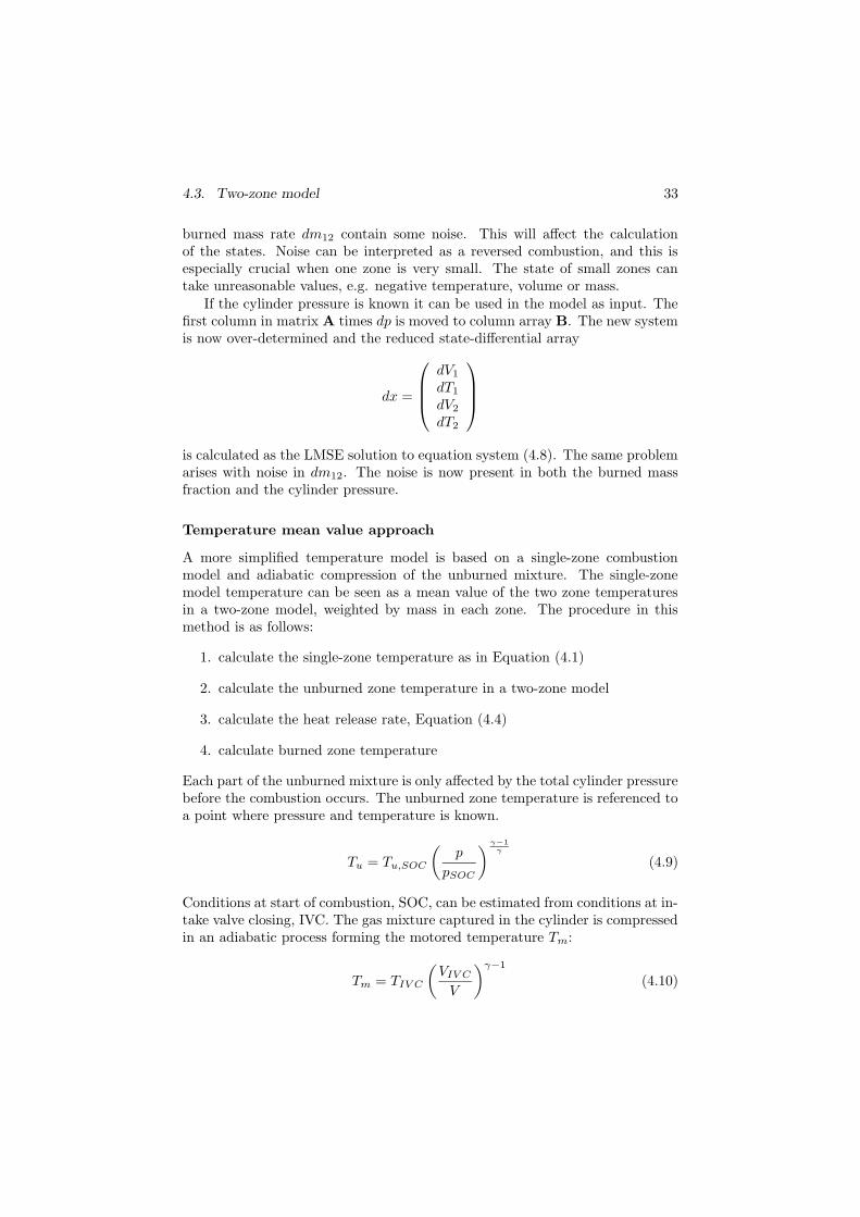
Figure 4.3: Zone temperatures and burned mass fraction for the temperaturemean value 2-zone model
The unburned zone shares the properties of the motored temperature at SOC.
Tu,SOC = Tm,SOC (4.11)
The burned mass fraction is calculated by Equation (4.7) The single-zone tem-perature T1zone is calculated as Equation (4.1) and is seen as the mass-weightedmean temperature of the two zones
T1zone =mbTb + muTu
mb + mu(4.12)
In this case the difference in specific heat capacity cv is neglected. Including amodel for cv would increase the importance of the burned gas temperature Tb.Equation (4.12) gives Tb as
Tb = T1zone(1 +mu
mb) − Tu
mu
mb(4.13)
The calculation of Tb is sensitive for low values of the burned mass fraction,mfb. As seen in Figure 4.3 the temperature calculation is unreliable for mfb< 0.01. In this case a temperature limitation of 2500 K, the adiabatic flametemperature, was set for mfb < 0.01. The reason for the unreliability is that mfband T1zone is calculated independently from each other, with no assumptions ofTb.
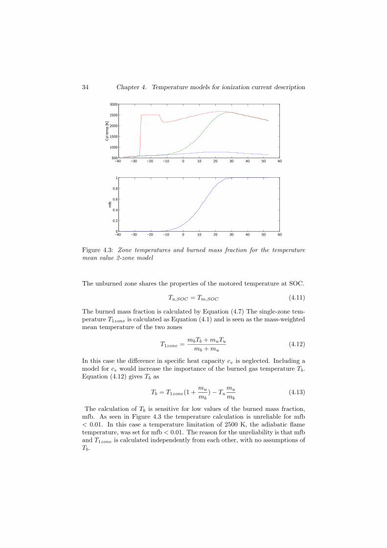
4.4. Temperature model evaluation 35
Combustionmodel
Saitzkoff−Reinmannmodel
NO formationZeldovich
Cyl P Ionisation CurrentZone Temp NO ratio
Figure 4.4: A view of the simulation process.
The burned zone volume, Vb, is calculated as
Vb =Tb mfb
mfb Tb + (1 − mfb)TuV (4.14)
where V is the total cylinder volume.
4.4 Temperature model evaluation
The temperature models are here evaluated in the point of view of how theyexplain the ionization current, assuming thermal ionization. To do that a sim-ulation model was designed according to Figure 4.4.
Simulation of ionization currents are based on pressure traces. A chainof calculations will finally lead to the ionization current as in Figure 4.4. Acombustion model uses the pressure trace to calculate the temperature for theburned gases of interest. Both the NO formation calculation and the ionizationcurrent simulation then use the temperature trace.
Section 3.2 summarizes the model presented by Saitzkoff et al. (1996), forthermal ionization of nitric oxide, NO. This model is based on the assumptionthat the main carriers are free electrons. The main generator for free electronsis the thermal ionization of nitric oxide. The model for the ionization currentlooks like
I = Uπr2
d
e2
σme
√
8kTπme
√
φs
√
√
√
√2(
2πmekTh2
)32 B1
B0exp
[
−E1
kT
]
ntot
where the parameters are listed in Table 4.1.
In this model there are three variables that are crank angle dependent; tem-perature T , particle density ntot and molar fraction of NO φs. Saitzkoff et al.(1996) made simulations based on a kernel-zone model and a fixed NO molar
36 Chapter 4. Temperature models for ionization current description
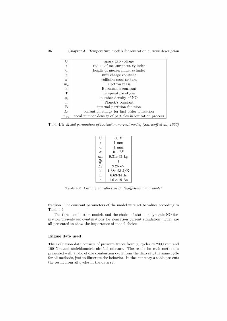
U spark gap voltager radius of measurement cylinderd length of measurement cylindere unit charge constantσ collision cross section
me electron massk Bolzmann’s constantT temperature of gasφs number density of NOh Planck’s constantB internal partition functionE1 ionization energy for first order ionizationntot total number density of particles in ionization process
Table 4.1: Model parameters of ionization current model, (Saitzkoff et al., 1996)
U 80 Vr 1 mmd 1 mmσ 0.1 A2
me 9.31e-31 kgB1
B01
E1 9.25 eVk 1.38e-23 J/Kh 6.63-34 Jse 1.6 e-19 As
Table 4.2: Parameter values in Saitzkoff-Reinmann model
fraction. The constant parameters of the model were set to values according toTable 4.2.
The three combustion models and the choice of static or dynamic NO for-mation presents six combinations for ionization current simulation. They areall presented to show the importance of model choice.
Engine data used
The evaluation data consists of pressure traces from 50 cycles at 2000 rpm and100 Nm and stoichiometric air fuel mixture. The result for each method ispresented with a plot of one combustion cycle from the data set, the same cyclefor all methods, just to illustrate the behavior. In the summary a table presentsthe result from all cycles in the data set.
4.4. Temperature model evaluation 37
−50 0 50 1000
0.5
1
1.5
2
2.5
3x 10
6
CA
Cyl
prs
−50 0 50 1000
500
1000
1500
2000
2500
CA
Cyl
Tem
p
−50 0 50 1001
1
1
1
1
1
1x 10
4
CA
NO
[ppm
]
−50 0 50 100−5
0
5
10x 10
−5
CA
Ion
@80
V [A
]
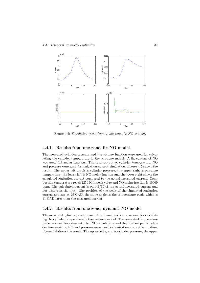
Figure 4.5: Simulation result from a one-zone, fix NO content.
4.4.1 Results from one-zone, fix NO model
The measured cylinder pressure and the volume function were used for calcu-lating the cylinder temperature in the one-zone model. A fix content of NOwas used, 1% molar fraction. The total output of cylinder temperature, NOand pressure were used for ionization current simulation. Figure 4.5 shows theresult. The upper left graph is cylinder pressure, the upper right is one-zonetemperature, the lower left is NO molar fraction and the lower right shows thecalculated ionization current compared to the actual measured current. Com-bustion temperature reach 2250 K in peak value and NO molar fraction is 10000ppm. The calculated current is only 1/16 of the actual measured current andnot visible in the plot. The position of the peak of the simulated ionizationcurrent appears at 29 CAD, the same angle as the temperature peak, which is11 CAD later than the measured current.
4.4.2 Results from one-zone, dynamic NO model
The measured cylinder pressure and the volume function were used for calculat-ing the cylinder temperature in the one-zone model. The generated temperaturetrace was used for rate-controlled NO calculations and the total output of cylin-der temperature, NO and pressure were used for ionization current simulation.Figure 4.6 shows the result. The upper left graph is cylinder pressure, the upper
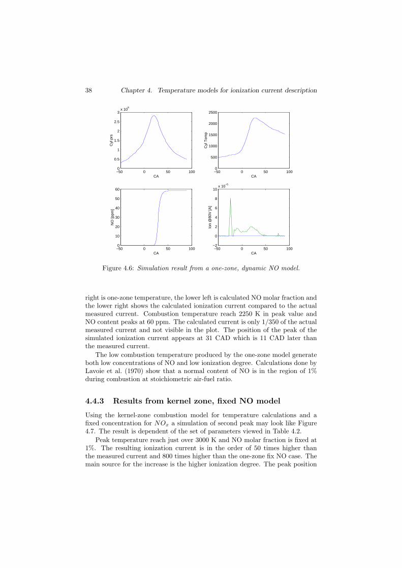
38 Chapter 4. Temperature models for ionization current description
−50 0 50 1000
0.5
1
1.5
2
2.5
3x 10
6
CA
Cyl
prs
−50 0 50 1000
500
1000
1500
2000
2500
CA
Cyl
Tem
p
−50 0 50 1000
10
20
30
40
50
60
CA
NO
[ppm
]
−50 0 50 100−2
0
2
4
6
8
10x 10
−5
CA
Ion
@80
V [A
]
Figure 4.6: Simulation result from a one-zone, dynamic NO model.
right is one-zone temperature, the lower left is calculated NO molar fraction andthe lower right shows the calculated ionization current compared to the actualmeasured current. Combustion temperature reach 2250 K in peak value andNO content peaks at 60 ppm. The calculated current is only 1/350 of the actualmeasured current and not visible in the plot. The position of the peak of thesimulated ionization current appears at 31 CAD which is 11 CAD later thanthe measured current.
The low combustion temperature produced by the one-zone model generateboth low concentrations of NO and low ionization degree. Calculations done byLavoie et al. (1970) show that a normal content of NO is in the region of 1%during combustion at stoichiometric air-fuel ratio.
4.4.3 Results from kernel zone, fixed NO model
Using the kernel-zone combustion model for temperature calculations and afixed concentration for NOx a simulation of second peak may look like Figure4.7. The result is dependent of the set of parameters viewed in Table 4.2.
Peak temperature reach just over 3000 K and NO molar fraction is fixed at1%. The resulting ionization current is in the order of 50 times higher thanthe measured current and 800 times higher than the one-zone fix NO case. Themain source for the increase is the higher ionization degree. The peak position
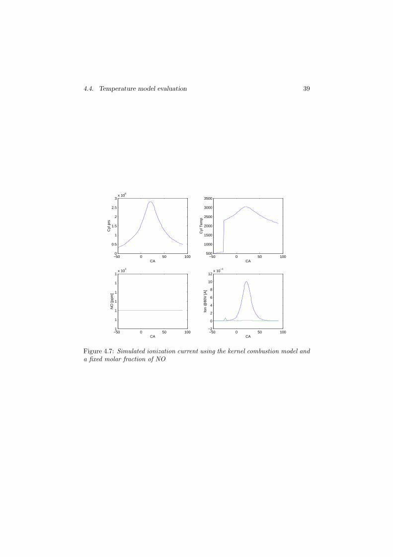
4.4. Temperature model evaluation 39
−50 0 50 1000
0.5
1
1.5
2
2.5
3x 10
6
CA
Cyl
prs
−50 0 50 100500
1000
1500
2000
2500
3000
3500
CA
Cyl
Tem
p
−50 0 50 1001
1
1
1
1
1
1x 10
4
CA
NO
[ppm
]
−50 0 50 100−2
0
2
4
6
8
10
12x 10
−4
CA
Ion
@80
V [A
]
Figure 4.7: Simulated ionization current using the kernel combustion model anda fixed molar fraction of NO
40 Chapter 4. Temperature models for ionization current description
−50 0 50 1000
0.5
1
1.5
2
2.5
3x 10
6
CA
Cyl
prs
−50 0 50 100500
1000
1500
2000
2500
3000
3500
CA
Cyl
Tem
p
−50 0 50 1000
2000
4000
6000
8000
10000
12000
14000
CA
NO
[ppm
]
−50 0 50 100−2
0
2
4
6
8
10
12x 10
−4
CA
Ion
@80
V [A
]
Figure 4.8: Simulation of ionization current from SAAB 9000 engine data.Simulated current is compared to the measured current.
of the current is at 21.5 CAD which is only 1.5 CAD later than the measuredcurrent peak.
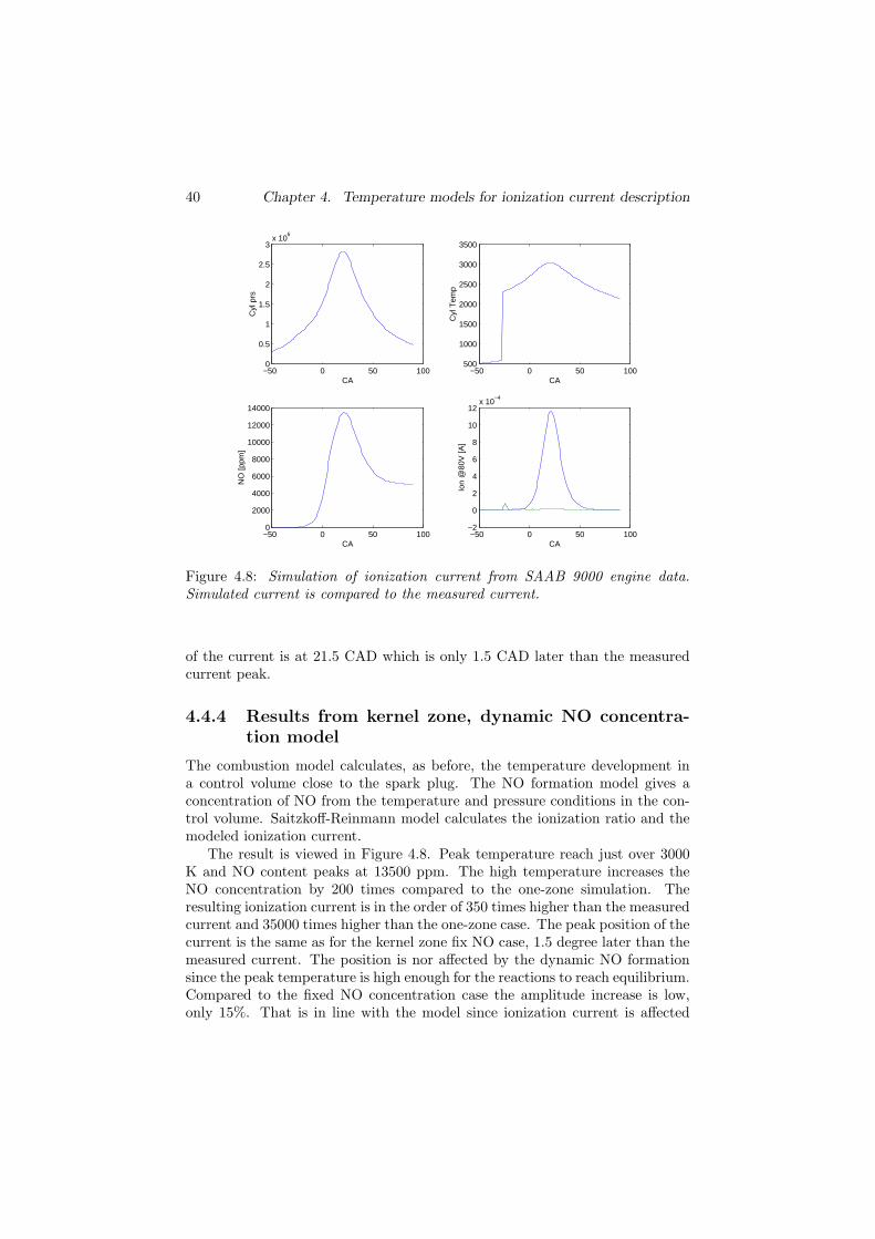
4.4.4 Results from kernel zone, dynamic NO concentra-
tion model
The combustion model calculates, as before, the temperature development ina control volume close to the spark plug. The NO formation model gives aconcentration of NO from the temperature and pressure conditions in the con-trol volume. Saitzkoff-Reinmann model calculates the ionization ratio and themodeled ionization current.
The result is viewed in Figure 4.8. Peak temperature reach just over 3000K and NO content peaks at 13500 ppm. The high temperature increases theNO concentration by 200 times compared to the one-zone simulation. Theresulting ionization current is in the order of 350 times higher than the measuredcurrent and 35000 times higher than the one-zone case. The peak position of thecurrent is the same as for the kernel zone fix NO case, 1.5 degree later than themeasured current. The position is nor affected by the dynamic NO formationsince the peak temperature is high enough for the reactions to reach equilibrium.Compared to the fixed NO concentration case the amplitude increase is low,only 15%. That is in line with the model since ionization current is affected
4.4. Temperature model evaluation 41
−50 0 50 1000
0.5
1
1.5
2
2.5
3x 10
6
CA
Cyl
prs
−50 0 50 100500
1000
1500
2000
2500
3000
CA
Cyl
Tem
p
−50 0 50 1001
1
1
1
1
1
1x 10
4
CA
NO
[ppm
]
−50 0 50 100−2
0
2
4
6
8
10x 10
−5
CA
Ion
@80
V [A
]
Figure 4.9: Simulated ionization current using the two-zone combustion modeland a fixed molar fraction of NO
by the square root of NO concentration, and that the ionization degree due totemperature is the same.
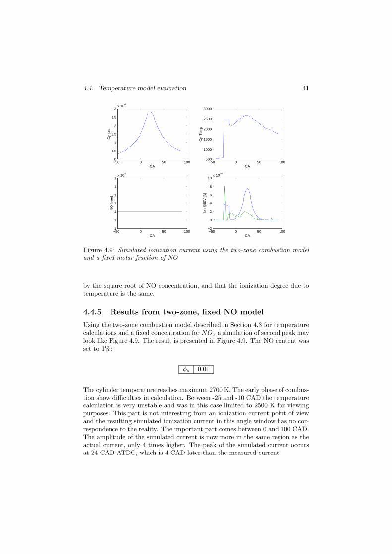
4.4.5 Results from two-zone, fixed NO model
Using the two-zone combustion model described in Section 4.3 for temperaturecalculations and a fixed concentration for NOx a simulation of second peak maylook like Figure 4.9. The result is presented in Figure 4.9. The NO content wasset to 1%:
φs 0.01
The cylinder temperature reaches maximum 2700 K. The early phase of combus-tion show difficulties in calculation. Between -25 and -10 CAD the temperaturecalculation is very unstable and was in this case limited to 2500 K for viewingpurposes. This part is not interesting from an ionization current point of viewand the resulting simulated ionization current in this angle window has no cor-respondence to the reality. The important part comes between 0 and 100 CAD.The amplitude of the simulated current is now more in the same region as theactual current, only 4 times higher. The peak of the simulated current occursat 24 CAD ATDC, which is 4 CAD later than the measured current.
42 Chapter 4. Temperature models for ionization current description
−50 0 50 1000
0.5
1
1.5
2
2.5
3x 10
6
CA
Cyl
prs
−50 0 50 100500
1000
1500
2000
2500
3000
CA
Cyl
Tem
p
−50 0 50 100−1000
0
1000
2000
3000
4000
5000
6000
CA
NO
[ppm
]
−50 0 50 100−2
0
2
4
6
8
10x 10
−5
CA
Ion
@80
V [A
]
Figure 4.10: Simulation of ionization current from SAAB 9000 engine data.Simulated current is compared to the measured current.
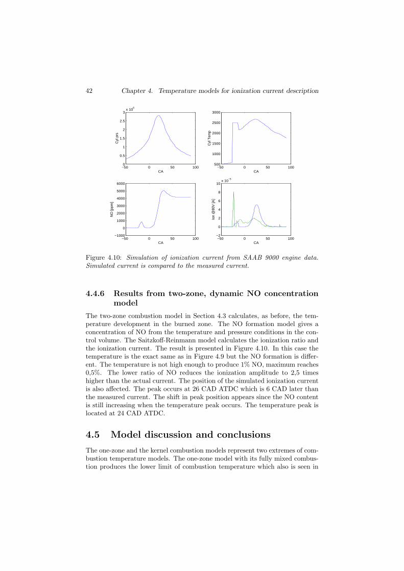
4.4.6 Results from two-zone, dynamic NO concentration
model
The two-zone combustion model in Section 4.3 calculates, as before, the tem-perature development in the burned zone. The NO formation model gives aconcentration of NO from the temperature and pressure conditions in the con-trol volume. The Saitzkoff-Reinmann model calculates the ionization ratio andthe ionization current. The result is presented in Figure 4.10. In this case thetemperature is the exact same as in Figure 4.9 but the NO formation is differ-ent. The temperature is not high enough to produce 1% NO, maximum reaches0,5%. The lower ratio of NO reduces the ionization amplitude to 2,5 timeshigher than the actual current. The position of the simulated ionization currentis also affected. The peak occurs at 26 CAD ATDC which is 6 CAD later thanthe measured current. The shift in peak position appears since the NO contentis still increasing when the temperature peak occurs. The temperature peak islocated at 24 CAD ATDC.
4.5 Model discussion and conclusions
The one-zone and the kernel combustion models represent two extremes of com-bustion temperature models. The one-zone model with its fully mixed combus-tion produces the lower limit of combustion temperature which also is seen in
4.5. Model discussion and conclusions 43
the simulated ionization current. The amplitude of the simulated current is onlya few percent of the actual measured one. The kernel model on the other hand,with its non-mixed burned gas kernel produces the upper limit of combustiontemperature. The amplitude of the simulated current is now some 50 timeshigher than the measured one. The two-zone model represents a middle coursebetween the two extremes.
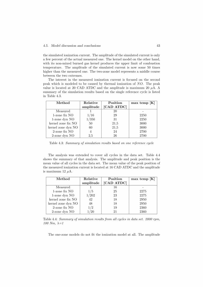
The interest in the measured ionization current is focused on the secondpeak which is modeled to be caused by thermal ionization of NO. The peakvalue is located at 20 CAD ATDC and the amplitude is maximum 20 µA. Asummary of the simulation results based on the single reference cycle is listedin Table 4.3.
Method Relative Position max temp [K]amplitude [CAD ATDC]
Measured 1 20 -1-zone fix NO 1/16 29 22501-zone dyn NO 1/350 31 2250
kernel zone fix NO 50 21,5 3000kernel zone dyn NO 60 21,5 3000
2-zone fix NO 4 24 27002-zone dyn NO 2,5 26 2700
Table 4.3: Summary of simulation results based on one reference cycle
The analysis was extended to cover all cycles in the data set. Table 4.4shows the summary of that analysis. The amplitude and peak position is themean value of all cycles in the data set. The mean value of the peak position ofthe measured ionization current is located at 16 CAD ATDC and the amplitudeis maximum 12 µA.
Method Relative Position max temp [K]amplitude [CAD ATDC]
Measured 1 16 -1-zone fix NO 1/5 25 22751-zone dyn NO 1/202 23 2275
kernel zone fix NO 42 18 2950kernel zone dyn NO 48 18 2950
2-zone fix NO 1/2 19 23602-zone dyn NO 1/20 21 2360
Table 4.4: Summary of simulation results from all cycles in data set. 2000 rpm,100 Nm, λ=1
The one-zone models do not fit the ionization model at all. The amplitude
44 Chapter 4. Temperature models for ionization current description
is only a few percent of the actual and the position is about 8 CAD late. Thekernel zone models present a high amplitude but the position is good, only 2CAD difference. The two-zone models present an amplitude that is slightly lowand a position that is later than the kernel model, 4 CAD from the measuredcurrent. By adjusting parameters in the thermal ionization model within phys-ically reasonable ranges it is possible to come closer to the actual amplitudelevel. For example, if the radius r of the measurement cylinder increases from1 to 1.5 mm, the amplitude increases 2.25 times.
Adding the dynamic NO formation process does not apparently improvethe model for one operating point since the same correction can be achievedthrough parameter calibration. However, I believe that the dynamic NO forma-tion modeling can contribute to a better model agreement when the operatingpoint is changed, e.g. for lean operation when the combustion temperature willdecrease and the formation process of NO gets more important.
The investigation shows how important the temperature model is for mod-eling the ionization current. The temperature has large impact on both NOcontent and ionization ratio. Earlier measurements done by Greenhalgh (1983)points at combustion peak temperatures of 2700-2800 K for stoichiometric toslightly rich operation. Lean operation decreases the combustion temperature.A combustion model that finds a peak temperature between the kernel modeland the two-zone model will both explain the combustion itself better and pro-duce an ionization current amplitude which is closer to the measurements.
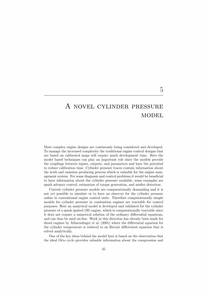
5
A novel cylinder pressure
model
More complex engine designs are continously being considered and developed.To manage the increased complexity the traditional engine control designs thatare based on calibrated maps will require much development time. Here themodel based techniques can play an important role since the models providethe couplings between inputs, outputs, and parameters and have the potentialto reduce calibration time. Cylinder pressure traces contain information aboutthe work and emission producing process which is valuable for the engine man-agement system. For some diagnosis and control problems it would be beneficialto have information about the cylinder pressure available, some examples arespark advance control, estimation of torque generation, and misfire detection.
Current cylinder pressure models are computationally demanding and it isnot yet possible to simulate or to have an observer for the cylinder pressureonline in conventional engine control units. Therefore computationally simplemodels for cylinder pressure in combustion engines are tractable for controlpurposes. Here an analytical model is developed and validated for the cylinderpressure of a spark ignited (SI) engine, which is computationally tractable sinceit does not require a numerical solution of the ordinary differential equations,and can thus be used on-line. Work in this direction has already been made fordiesel engines by Allmendinger et al. (2001) where the differential equation forthe cylinder temperature is reduced to an Riccati differential equation that issolved analytically.
One of the key ideas behind the model here is based on the observation thatthe ideal Otto cycle provides valuable information about the compression and
45
46 Chapter 5. A novel cylinder pressure model
expansion processes. These two processes are seen in the real measured pressuretraces under normal operating conditions as the asymptotes before the ignitionand after the combustion is finished. The real cycle is similar to the ideal Ottocycle and the similarities are largest early in the compression and late in theexpansion. It is characterized by the compression and expansion phases whichare well defined by the states of the fluid. The second key idea is that the heatrelease analysis procedure based on pressure ratio management, developed byMatekunas (Matekunas, 1986, 1984, 1983), gives a good approximation of theheat release trace. This method can easily be inverted and used to interpolatebetween the compression and expansion trace.
The model is described using measurements readily available in productionengines and using a set of tuning parameters that have physical interpreta-tions and are closely connected to the ideal Otto cycle. This work focuses oninvestigating the accuracy of the simple model, not on how parameters canbe determined or predicted. The interesting question is, how well the simplemodel describes the in-cylinder pressure during the high pressure and combus-tion phase. The burn rate of the combustion has a big influence on the pressureand in the validation the burn rate is considered to be known. However, thereare several approaches presented for estimating the burn rate which could beused directly in this model. Two slightly different approaches are describedby Csallner (1980); Hires et al. (1978) that present ways of predicting the vari-ations of the burn angles over the full engine operating range by utilizing areference measurement in a central area of the operating point. Another ap-proach is described by Daniels (1998) which is based on the ionization currentmeasurements, this approach is also applicable since the ion current has beenused in production cars since 1994, see e.g. Auzins et al. (1995).
5.1 Model description
Figure 5.1 outlines the ideas behind and the structure within the model. Themodeled pressure trace p(θ) is built up by two asymptotic traces and an in-terpolation between these. The cylinder pressure model is divided into fourparts:
• The compression process is well described by a polytropic process. Thepolytropic process also encapsulates the heat transfer, so that there is noneed to explicitly include the heat transfer in the model.
• The expansion asymptote is also well described by a polytropic process.The reference point for expansion temperature and pressure is calculatedusing a constant-volume combustion process.
• The concept of pressure ratio management provides a convenient way tointerpolate from compression to expansion. Its appearance is very close tothe mass fraction burned profile and the Vibe function is used to describethe pressure ratio.
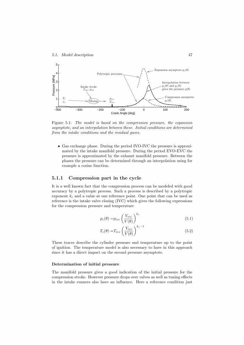
5.1. Model description 47
−400 −300 −200 −100 0 100 2000
1
2
3
4
5
Crank Angle [deg]
Pre
ssur
e [M
Pa]
pe(θ) and pc(θ)Interpolation between
gives the pressure p(θ)
Mixing
Compresson asymptotepivc
Tivc
Tr
xr
Intake stroke
Polytropic processes
Expansion asymptote pe(θ)
pc(θ)
Tim, pim
Figure 5.1: The model is based on the compression pressure, the expansionasymptote, and an interpolation between these. Initial conditions are determinedfrom the intake conditions and the residual gases.
• Gas exchange phase. During the period IVO-IVC the pressure is approxi-mated by the intake manifold pressure. During the period EVO-EVC thepressure is approximated by the exhaust manifold pressure. Between thephases the pressure can be determined through an interpolation using forexample a cosine function.
5.1.1 Compression part in the cycle
It is a well known fact that the compression process can be modeled with goodaccuracy by a polytropic process. Such a process is described by a polytropicexponent kc and a value at one reference point. One point that can be used asreference is the intake valve closing (IVC) which gives the following expressionsfor the compression pressure and temperature
pc(θ) =pivc
(
Vivc
V (θ)
)kc
(5.1)
Tc(θ) =Tivc
(
Vivc
V (θ)
)kc−1
(5.2)
These traces describe the cylinder pressure and temperature up to the pointof ignition. The temperature model is also necessary to have in this approachsince it has a direct impact on the second pressure asymptote.
Determination of initial pressure
The manifold pressure gives a good indication of the initial pressure for thecompression stroke. However pressure drops over valves as well as tuning effectsin the intake runners also have an influence. Here a reference condition just
48 Chapter 5. A novel cylinder pressure model
before IVC is used to determine the initial pressure
pivc = pim(θivc)
The crank angle for intake valve closing θivc is not exactly known due to produc-tion tolerances, it is also used as tuning parameter to compensate for pressuredrops over the valves etc. Additionally an affine correction in engine speed istested which improves the accuracy of the compression pressure model slightly,
pivc = pim(θivc) + c1 + c2 ∗ N
Here c1 and c2 are parameters that have to be determined which increases theflexibility but also the model complexity. To maintain simplicity the evaluationis concentrated on the first model.
Determination of initial temperature
It is more difficult to determine the fluid temperature at intake valve closingcompared to the pressure, since it is influenced by heat transfer and residualgases that are difficult to measure and determine. The air in the intake manifoldis heated from Tim to Ta by the hot valves and the locally high heat transfercoefficients in the cylinder. Fuel is added in the ports and undergoes an evapora-tion which also influences the temperature. By considering the energy equationwith a lumped process for heating, evaporation, and mixing, the initial air/fuelmixture temperature can be stated as
Taf =ma cp,a Ta + mf cp,f Tf − mf hv,f + Q
ma cp,a + mf cp,f
where hv,f is the vaporization enthalpy for the fuel and Q is the heat addedto the fresh mixture. Both these are difficult to determine. In the cylinder thefresh charge is mixed with the residual gases and the mixture temperature is
Tivc =maf cp,af Taf − mr cp,r Tr
maf cp,af − mr cp,r
Prior to mixing the residual gases are cooled down by heat transfer to the walls.
Simplifying the temperature model
The outlined models for heating, evaporation, and mixing processes are complexand contain several variables that have to be determined. The central questionhere is to see how well a simple model can capture the process and thereforesome simplifications are made. First it is assumed that the specific heats cp arethe same for the residual gas and the fresh air and fuel mixture yields
Tivc = Taf (1 − xr) + xr Tr (5.3)
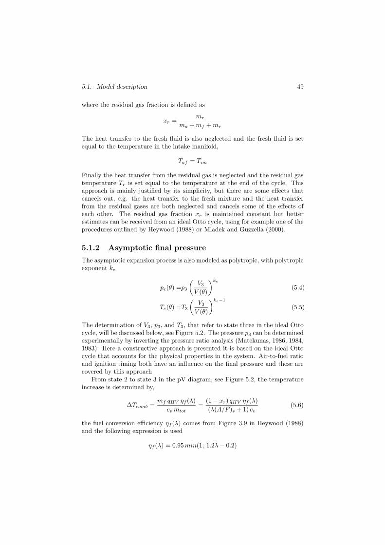
5.1. Model description 49
where the residual gas fraction is defined as
xr =mr
ma + mf + mr
The heat transfer to the fresh fluid is also neglected and the fresh fluid is setequal to the temperature in the intake manifold,
Taf = Tim
Finally the heat transfer from the residual gas is neglected and the residual gastemperature Tr is set equal to the temperature at the end of the cycle. Thisapproach is mainly justified by its simplicity, but there are some effects thatcancels out, e.g. the heat transfer to the fresh mixture and the heat transferfrom the residual gases are both neglected and cancels some of the effects ofeach other. The residual gas fraction xr is maintained constant but betterestimates can be received from an ideal Otto cycle, using for example one of theprocedures outlined by Heywood (1988) or Mladek and Guzzella (2000).
5.1.2 Asymptotic final pressure
The asymptotic expansion process is also modeled as polytropic, with polytropicexponent ke
pe(θ) =p3
(
V3
V (θ)
)ke
(5.4)
Te(θ) =T3
(
V3
V (θ)
)ke−1
(5.5)
The determination of V3, p3, and T3, that refer to state three in the ideal Ottocycle, will be discussed below, see Figure 5.2. The pressure p3 can be determinedexperimentally by inverting the pressure ratio analysis (Matekunas, 1986, 1984,1983). Here a constructive approach is presented it is based on the ideal Ottocycle that accounts for the physical properties in the system. Air-to-fuel ratioand ignition timing both have an influence on the final pressure and these arecovered by this approach
From state 2 to state 3 in the pV diagram, see Figure 5.2, the temperatureincrease is determined by,
∆Tcomb =mf qHV ηf (λ)
cv mtot=
(1 − xr) qHV ηf (λ)
(λ(A/F )s + 1) cv(5.6)
the fuel conversion efficiency ηf (λ) comes from Figure 3.9 in Heywood (1988)and the following expression is used
ηf (λ) = 0.95min(1; 1.2λ − 0.2)
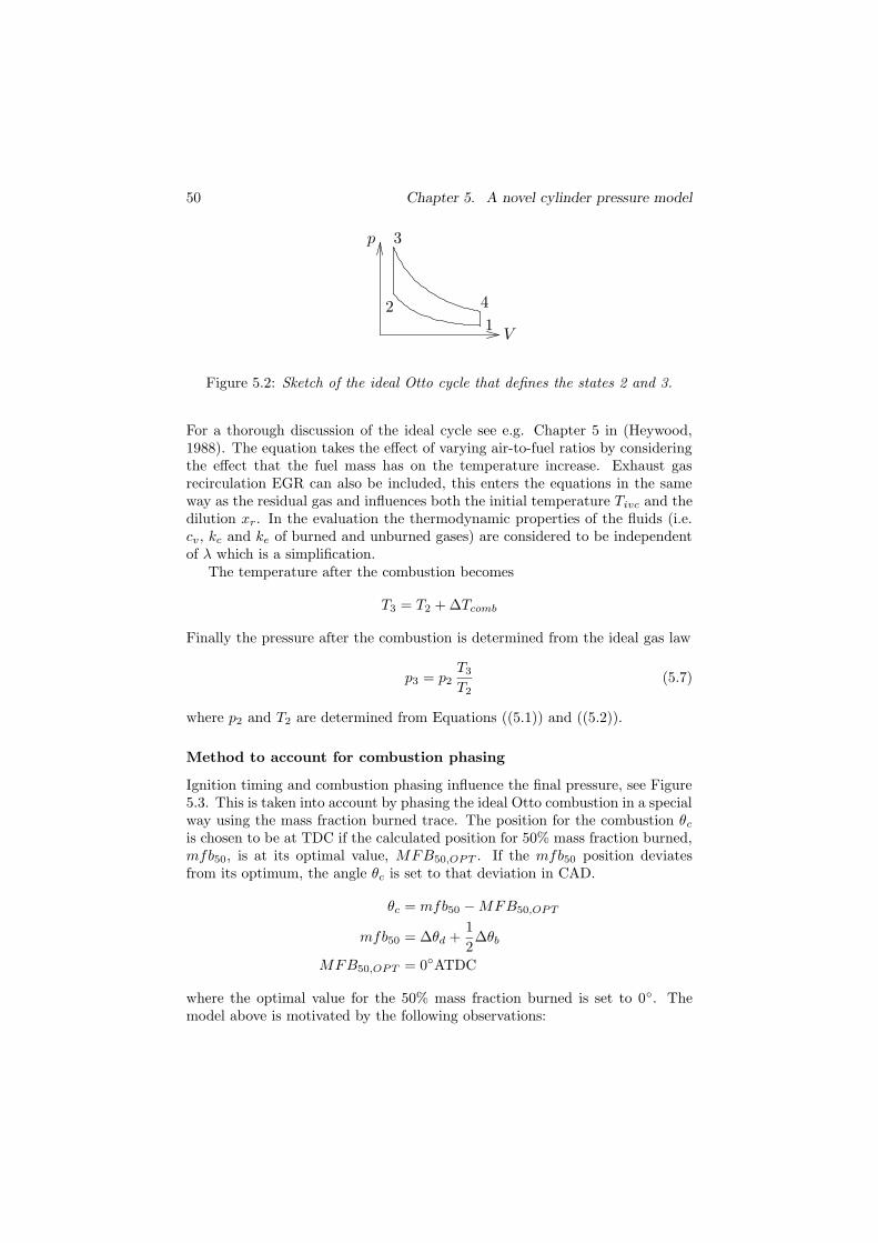
50 Chapter 5. A novel cylinder pressure model
1
p
V
3
2 4
Figure 5.2: Sketch of the ideal Otto cycle that defines the states 2 and 3.
For a thorough discussion of the ideal cycle see e.g. Chapter 5 in (Heywood,1988). The equation takes the effect of varying air-to-fuel ratios by consideringthe effect that the fuel mass has on the temperature increase. Exhaust gasrecirculation EGR can also be included, this enters the equations in the sameway as the residual gas and influences both the initial temperature Tivc and thedilution xr. In the evaluation the thermodynamic properties of the fluids (i.e.cv, kc and ke of burned and unburned gases) are considered to be independentof λ which is a simplification.
The temperature after the combustion becomes
T3 = T2 + ∆Tcomb
Finally the pressure after the combustion is determined from the ideal gas law
p3 = p2T3
T2(5.7)
where p2 and T2 are determined from Equations ((5.1)) and ((5.2)).
Method to account for combustion phasing
Ignition timing and combustion phasing influence the final pressure, see Figure5.3. This is taken into account by phasing the ideal Otto combustion in a specialway using the mass fraction burned trace. The position for the combustion θc
is chosen to be at TDC if the calculated position for 50% mass fraction burned,mfb50, is at its optimal value, MFB50,OPT . If the mfb50 position deviatesfrom its optimum, the angle θc is set to that deviation in CAD.
θc = mfb50 − MFB50,OPT
mfb50 = ∆θd +1
2∆θb
MFB50,OPT = 0◦ATDC
where the optimal value for the 50% mass fraction burned is set to 0◦. Themodel above is motivated by the following observations:
5.1. Model description 51
−60 −40 −20 0 20 40 60 80 1000
0.5
1
1.5
2
2.5
3
3.5
SA1
SA2
SA3
SA4
SA1
SA2
SA3
SA4
TDC
Pres
sure
[M
Pa]
Crank angle [deg]
−50 0 50 1000
0.2
0.4
0.6
0.8
1
CAD
MF
B
mfb50
MFB Vibe function
Figure 5.3: Left: Cylinder pressure from four cycles with different ignition tim-ing. Late combustion gives a higher expansion pressure asymptote. Right: Def-inition of mfb50. Heat release according to a Vibe function.
• The cycle with the best combustion phasing has best efficiency and lowestexhaust temperature.
• The best phased real cycles have their 50% mass fraction burned positionaround 8◦ ATDC. However, the experiments showed that MFB50,OPT =0o ATDC was a better selection.
• The Otto cycle has the best efficiency and lowest exhaust temperature ifthe combustion is at TDC.
These statements couple the mass fraction burned trace to θc in the ideal Ottocycle that defines the volumes at states 2 and 3 to V2 = V3 = V (θc).
5.1.3 Combustion part
The pressure ratio management has been investigated in great detail by Mateku-nas (Matekunas, 1986, 1984, 1983). The pressure ratio is defined using the ratiobetween the pressure from a firing cycle, p(θ), and the pressure from a motoredcycle, pc(θ),
PR(θ) =p(θ)
pc(θ)− 1 (5.8)
Traces produced by the pressure ratio are similar to the mass fraction burned
profiles, for example the position for PR(θ)max(PR(θ)) = 0.5 differs only around 1−2◦
from the position for 50% mass fraction burned (Eriksson, 1998). This impliesthat similar techniques for representing the mass fraction burned profile can beused to simulate the pressure, and this is the method that we have used.
52 Chapter 5. A novel cylinder pressure model
definition∆θd 0-10% burned mass fraction∆θb 10-85% burned mass fraction
Table 5.1: Definition of burn angles.
Interpolation method
The combustion part is produced by interpolating between the two assymptoticpressure traces pc and pe. The interpolation function is the well known Vibefunction (Vibe, 1970)
PR(θ) = 1 − e−a
(
θ−θSOC∆θ
)m+1
(5.9)
which gives the following expression for the pressure
p(θ) = (1 − PR(θ)) · pc(θ) + PR(θ) · pe(θ)
From the end of combustion to EVO the pressure follows the expansion asymp-tote, Equation (5.4).
The burn duration ∆θ and shape factors a and m in the Vibe functiondepend on engine speed, air-fuel ratio and EGR ratio. The work presented in(Csallner, 1980; Hires et al., 1978) develop models that addresses these issues.Here these variations are not considered, instead the parameters are specifiedin terms of the burn angles ∆θd, ∆θb. The burn angles are defined in Table 5.1.Given the burn angles the shape parameters a and m can be calculated theapproach here is the same as the one used by Eriksson (1999)
m =ln
(
ln(1−0.1)ln(1−0.85)
)
ln(∆θd) − ln(∆θd + ∆θb)− 1 (5.10)
a = − ln(1 − 0.1)
(
∆θ
∆θd
)m+1
(5.11)
Burn duration can be calculated using flame development angle, ∆θd, and fastburn angle, ∆θb.
∆θ ≈ 2∆θd + ∆θb (5.12)
5.1.4 The remaining parts of the cycle
After the exhaust valve has opened the blow-down phase begins and the pressureapproaches the pressure in the exhaust system. For this phase an interpolationscheme can also be used. The same goes for the phase after the intake valvehas opened and the cylinder pressure approaches the intake manifold pressure.For the transitions between these two phases a cosine function can be used forthe interpolation. These phases are not validated.
5.2. Model evaluation 53
5.1.5 Model parameters and inputs
The model is described by a set of inputs and a set of parameters that havephysical interpretation. These inputs and parameters are summarized in thissection. The tuning parameters are
cv specific heat at the combustionkc polytropic coefficient for the compression pressureke polytropic coefficient for the expansion pressure
qHV heating value for the fuel(A/F )s stoichometric air-fuel mass ratio
Tr residual gas temperaturexr residual gas fractionθivc intake valve closing angleθevo exhaust valve closing angle
MFB50,OPT optimum position of 50% burned mass fraction
The inputs are
pim intake manifold pressureTim intake manifold temperature∆θd flame development angle∆θb fast burn angleθSOC start of combustion angle
λ normalized air to fuel ratio
Tr and the residual gas fraction xr are used as tuning parameter here butthey can also be modeled, for example based on cycle simulations. They areimportant for the model since they directly influence the initial temperatureTivc, Equation (5.3), and the expansion pressure through Equations (5.2) and(5.7). An illustrative example: xr = 0.07, Tim = 298 [K], Tr = 1000 [K] yieldan initial temperature of Tivc = 347 [K], which is a 16% increase. This effect isdirectly visible in the expansion pressure asymptote.
5.2 Model evaluation
The model consists of a set of parts of which the following will be validated
1. selection of compression pressure
2. selection of compression and expansion polytropic coefficient
3. selection of expansion pressure
4. interpolation between firing and expansion
Finally the influence from air-fuel ratio and ignition timing is studied.
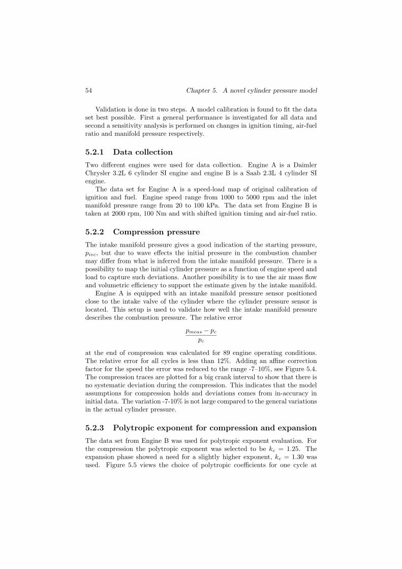
54 Chapter 5. A novel cylinder pressure model
Validation is done in two steps. A model calibration is found to fit the dataset best possible. First a general performance is investigated for all data andsecond a sensitivity analysis is performed on changes in ignition timing, air-fuelratio and manifold pressure respectively.
5.2.1 Data collection
Two different engines were used for data collection. Engine A is a DaimlerChrysler 3.2L 6 cylinder SI engine and engine B is a Saab 2.3L 4 cylinder SIengine.
The data set for Engine A is a speed-load map of original calibration ofignition and fuel. Engine speed range from 1000 to 5000 rpm and the inletmanifold pressure range from 20 to 100 kPa. The data set from Engine B istaken at 2000 rpm, 100 Nm and with shifted ignition timing and air-fuel ratio.
5.2.2 Compression pressure
The intake manifold pressure gives a good indication of the starting pressure,pivc, but due to wave effects the initial pressure in the combustion chambermay differ from what is inferred from the intake manifold pressure. There is apossibility to map the initial cylinder pressure as a function of engine speed andload to capture such deviations. Another possibility is to use the air mass flowand volumetric efficiency to support the estimate given by the intake manifold.
Engine A is equipped with an intake manifold pressure sensor positionedclose to the intake valve of the cylinder where the cylinder pressure sensor islocated. This setup is used to validate how well the intake manifold pressuredescribes the combustion pressure. The relative error
pmeas − pc
pc
at the end of compression was calculated for 89 engine operating conditions.The relative error for all cycles is less than 12%. Adding an affine correctionfactor for the speed the error was reduced to the range -7–10%, see Figure 5.4.The compression traces are plotted for a big crank interval to show that there isno systematic deviation during the compression. This indicates that the modelassumptions for compression holds and deviations comes from in-accuracy ininitial data. The variation -7-10% is not large compared to the general variationsin the actual cylinder pressure.
5.2.3 Polytropic exponent for compression and expansion
The data set from Engine B was used for polytropic exponent evaluation. Forthe compression the polytropic exponent was selected to be kc = 1.25. Theexpansion phase showed a need for a slightly higher exponent, ke = 1.30 wasused. Figure 5.5 views the choice of polytropic coefficients for one cycle at
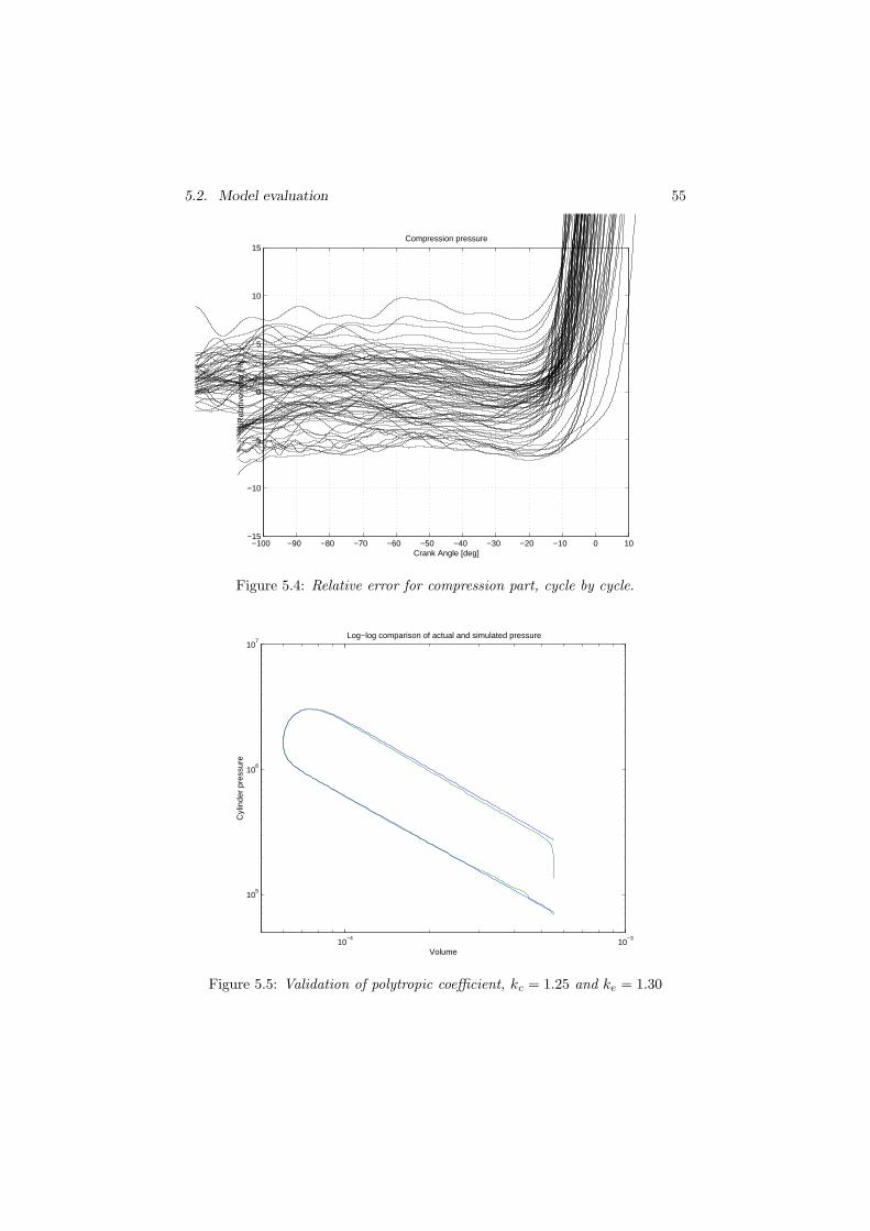
5.2. Model evaluation 55
−100 −90 −80 −70 −60 −50 −40 −30 −20 −10 0 10−15
−10
−5
0
5
10
15
Crank Angle [deg]
Rel
ativ
e er
ror
[%]
Compression pressure
Figure 5.4: Relative error for compression part, cycle by cycle.
10−4
10−3
105
106
107
Volume
Cyl
inde
r pr
essu
re
Log−log comparison of actual and simulated pressure
Figure 5.5: Validation of polytropic coefficient, kc = 1.25 and ke = 1.30
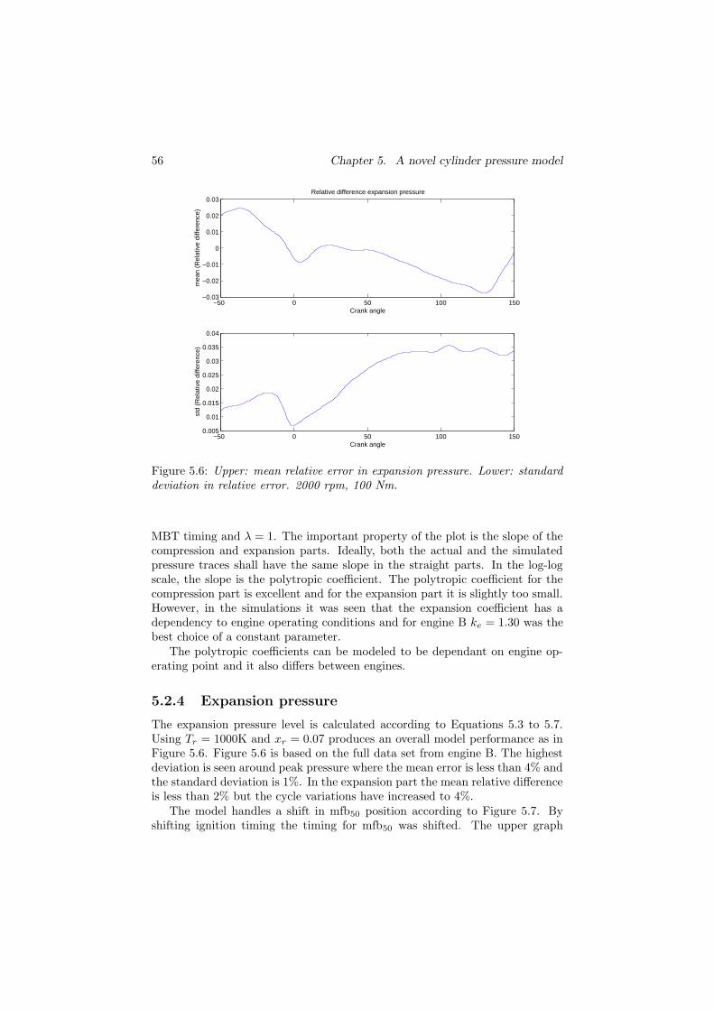
56 Chapter 5. A novel cylinder pressure model
−50 0 50 100 150−0.03
−0.02
−0.01
0
0.01
0.02
0.03
Crank angle
mea
n (R
elat
ive
diffe
renc
e)Relative difference expansion pressure
−50 0 50 100 1500.005
0.01
0.015
0.02
0.025
0.03
0.035
0.04
Crank angle
std
(Rel
ativ
e di
ffere
nce)
Figure 5.6: Upper: mean relative error in expansion pressure. Lower: standarddeviation in relative error. 2000 rpm, 100 Nm.
MBT timing and λ = 1. The important property of the plot is the slope of thecompression and expansion parts. Ideally, both the actual and the simulatedpressure traces shall have the same slope in the straight parts. In the log-logscale, the slope is the polytropic coefficient. The polytropic coefficient for thecompression part is excellent and for the expansion part it is slightly too small.However, in the simulations it was seen that the expansion coefficient has adependency to engine operating conditions and for engine B ke = 1.30 was thebest choice of a constant parameter.
The polytropic coefficients can be modeled to be dependant on engine op-erating point and it also differs between engines.
5.2.4 Expansion pressure
The expansion pressure level is calculated according to Equations 5.3 to 5.7.Using Tr = 1000K and xr = 0.07 produces an overall model performance as inFigure 5.6. Figure 5.6 is based on the full data set from engine B. The highestdeviation is seen around peak pressure where the mean error is less than 4% andthe standard deviation is 1%. In the expansion part the mean relative differenceis less than 2% but the cycle variations have increased to 4%.
The model handles a shift in mfb50 position according to Figure 5.7. Byshifting ignition timing the timing for mfb50 was shifted. The upper graph
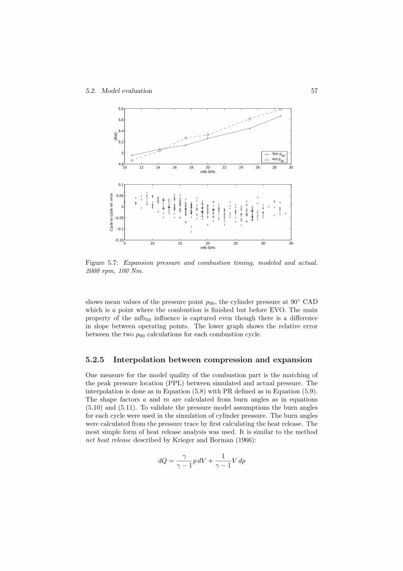
5.2. Model evaluation 57
10 12 14 16 18 20 22 24 26 28 304.8
5
5.2
5.4
5.6
5.8
mfb 50%
[Bar
]
Sim p90
Act p90
5 10 15 20 25 30 35−0.15
−0.1
−0.05
0
0.05
0.1
mfb 50%
Cyc
le to
cyc
le r
el. e
rror
Figure 5.7: Expansion pressure and combustion timing, modeled and actual.2000 rpm, 100 Nm.
shows mean values of the pressure point p90, the cylinder pressure at 90◦ CADwhich is a point where the combustion is finished but before EVO. The mainproperty of the mfb50 influence is captured even though there is a differencein slope between operating points. The lower graph shows the relative errorbetween the two p90 calculations for each combustion cycle.
5.2.5 Interpolation between compression and expansion
One measure for the model quality of the combustion part is the matching ofthe peak pressure location (PPL) between simulated and actual pressure. Theinterpolation is done as in Equation (5.8) with PR defined as in Equation (5.9).The shape factors a and m are calculated from burn angles as in equations(5.10) and (5.11). To validate the pressure model assumptions the burn anglesfor each cycle were used in the simulation of cylinder pressure. The burn angleswere calculated from the pressure trace by first calculating the heat release. Themost simple form of heat release analysis was used. It is similar to the methodnet heat release described by Krieger and Borman (1966):
dQ =γ
γ − 1p dV +
1
γ − 1V dp
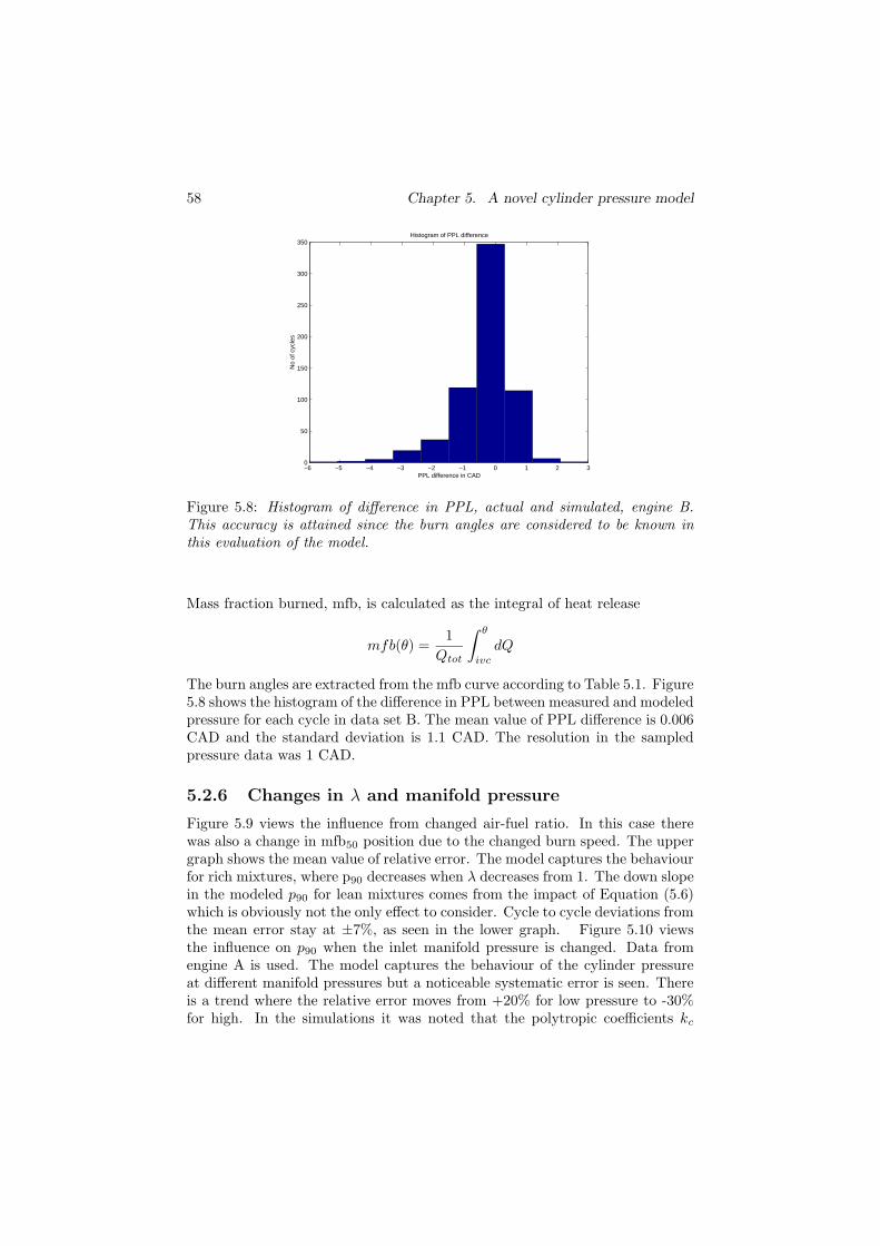
58 Chapter 5. A novel cylinder pressure model
−6 −5 −4 −3 −2 −1 0 1 2 30
50
100
150
200
250
300
350
PPL difference in CAD
No
of c
ycle
s
Histogram of PPL difference
Figure 5.8: Histogram of difference in PPL, actual and simulated, engine B.This accuracy is attained since the burn angles are considered to be known inthis evaluation of the model.
Mass fraction burned, mfb, is calculated as the integral of heat release
mfb(θ) =1
Qtot
∫ θ
ivc
dQ
The burn angles are extracted from the mfb curve according to Table 5.1. Figure5.8 shows the histogram of the difference in PPL between measured and modeledpressure for each cycle in data set B. The mean value of PPL difference is 0.006CAD and the standard deviation is 1.1 CAD. The resolution in the sampledpressure data was 1 CAD.
5.2.6 Changes in λ and manifold pressure
Figure 5.9 views the influence from changed air-fuel ratio. In this case therewas also a change in mfb50 position due to the changed burn speed. The uppergraph shows the mean value of relative error. The model captures the behaviourfor rich mixtures, where p90 decreases when λ decreases from 1. The down slopein the modeled p90 for lean mixtures comes from the impact of Equation (5.6)which is obviously not the only effect to consider. Cycle to cycle deviations fromthe mean error stay at ±7%, as seen in the lower graph. Figure 5.10 viewsthe influence on p90 when the inlet manifold pressure is changed. Data fromengine A is used. The model captures the behaviour of the cylinder pressureat different manifold pressures but a noticeable systematic error is seen. Thereis a trend where the relative error moves from +20% for low pressure to -30%for high. In the simulations it was noted that the polytropic coefficients kc
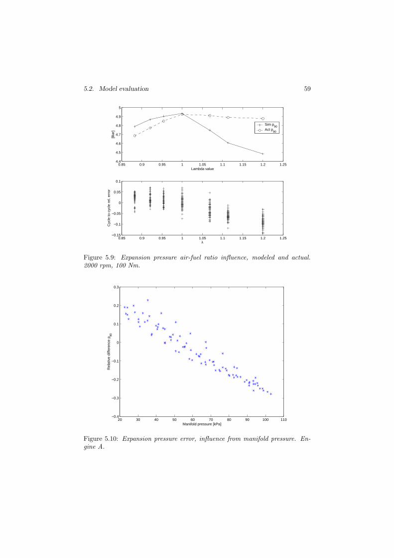
5.2. Model evaluation 59
0.85 0.9 0.95 1 1.05 1.1 1.15 1.2 1.254.4
4.5
4.6
4.7
4.8
4.9
5
Lambda value
[Bar
]
Sim p90
Act p90
0.85 0.9 0.95 1 1.05 1.1 1.15 1.2 1.25−0.15
−0.1
−0.05
0
0.05
0.1
λ
Cyc
le to
cyc
le r
el. e
rror
Figure 5.9: Expansion pressure air-fuel ratio influence, modeled and actual.2000 rpm, 100 Nm.
20 30 40 50 60 70 80 90 100 110−0.4
−0.3
−0.2
−0.1
0
0.1
0.2
0.3
Manifold pressure [kPa]
Rel
ativ
e di
ffere
nce
p 90
Figure 5.10: Expansion pressure error, influence from manifold pressure. En-gine A.
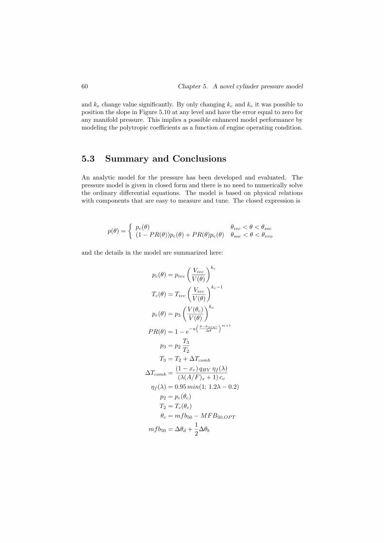
60 Chapter 5. A novel cylinder pressure model
and ke change value significantly. By only changing kc and ke it was possible toposition the slope in Figure 5.10 at any level and have the error equal to zero forany manifold pressure. This implies a possible enhanced model performance bymodeling the polytropic coefficients as a function of engine operating condition.
5.3 Summary and Conclusions
An analytic model for the pressure has been developed and evaluated. Thepressure model is given in closed form and there is no need to numerically solvethe ordinary differential equations. The model is based on physical relationswith components that are easy to measure and tune. The closed expression is
p(θ) =
{
pc(θ) θivc < θ < θsoc
(1 − PR(θ))pc(θ) + PR(θ)pe(θ) θsoc < θ < θevo
and the details in the model are summarized here:
pc(θ) = pivc
(
Vivc
V (θ)
)kc
Tc(θ) = Tivc
(
Vivc
V (θ)
)kc−1
pe(θ) = p3
(
V (θc)
V (θ)
)ke
PR(θ) = 1 − e−a
(
θ−θSOC∆θ
)m+1
p3 = p2T3
T2
T3 = T2 + ∆Tcomb
∆Tcomb =(1 − xr) qHV ηf (λ)
(λ(A/F )s + 1) cv
ηf (λ) = 0.95min(1; 1.2λ − 0.2)
p2 = pc(θc)
T2 = Tc(θc)
θc = mfb50 − MFB50,OPT
mfb50 = ∆θd +1
2∆θb
5.3. Summary and Conclusions 61
Tivc = Taf (1 − xr) + xr Tr
Vivc = V (θivc)
pivc = pim(θivc)
∆θ = 2∆θd + ∆θb
θsoc = θign
m =ln
(
ln(1−0.1)ln(1−0.85)
)
ln(∆θd) − ln(∆θd + ∆θb)− 1
a = − ln(1 − 0.1)
(
∆θ
∆θd
)m+1
Taf = Tim
The model contains a number of tuning parameters that effect the accuracy ofthe pressure model. The tuning parameters are
cv specific heat at the combustionkc polytropic coefficient for the compression pressureke polytropic coefficient for the expansion pressure
qHV heating value for the fuel(A/F )s stoichiometric air-fuel mass ratio
Tr residual gas temperaturexr residual gas fractionθivc intake valve closing angleθevo exhaust valve closing angle
MFB50,OPT optimum position of 50% burned mass fraction
The inputs are
pim intake manifold pressureTim intake manifold temperature∆θd flame development angle∆θb fast burn angleθign ignition angleλ normalized air to fuel ratio
With a proper tuning of these parameters it is shown that:
• Compression and expansion slopes can be captured well with an accuracyof -7 - 10%.
• When the burn angles are available for the model the peak pressure loca-tion stayed within ±1◦ standard deviation from the actual peak pressurelocation.
• The model can capture large variations in ignition timing.

62 Chapter 5. A novel cylinder pressure model
• The model can capture variations in air to fuel ratio in the rich region.
• Variations in manifold pressure are captured but a significant error trendis seen.
6
A parameterized ionization
current model
The parameterized pressure model, described in Chapter 5 gives together with atemperature model an opportunity to study combustion properties by analyzingthe ionization current. The focus here is set on the second or the thermal peakof the ionization current. A model is defined with a number of free parameters,which can be estimated by fitting the model to a selected part of a measuredionization current. The model has many parameters where all of them have aphysical interpretation. Here, two parameters are chosen to be free, to allowthe model to fit to the measured current. The rest of the model parameters arefixed to their best physical value. The two free parameters control position andamplitude of the ionization current.
6.1 Model description
6.1.1 Data collection
A 2.0 liter turbo charged gasoline engine was used for data collection. Data wascollected at 2000 rpm with a scan in air-fuel ratio and ignition timing accordingto Table 6.1. At each operating point (OP) 50 cycles of ionization current andcylinder pressure were recorded. MBTT is the ignition timing for maximumbrake torque. This data set was also used for the pressure model validation inChapter 5.
63
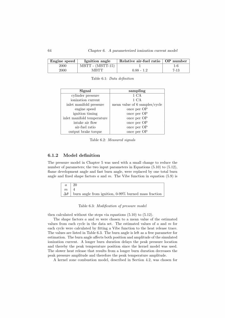
64 Chapter 6. A parameterized ionization current model
Engine speed Ignition angle Relative air-fuel ratio OP number2000 MBTT - (MBTT-15) 1 1-62000 MBTT 0.88 - 1.2 7-13
Table 6.1: Data definition
Signal samplingcylinder pressure 1 CAionization current 1 CA
inlet manifold pressure mean value of 6 samples/cycleengine speed once per OP
ignition timing once per OPinlet manifold temperature once per OP
intake air flow once per OPair-fuel ratio once per OP
output brake torque once per OP
Table 6.2: Measured signals
6.1.2 Model definition
The pressure model in Chapter 5 was used with a small change to reduce thenumber of parameters; the two input parameters in Equations (5.10) to (5.12),flame development angle and fast burn angle, were replaced by one total burnangle and fixed shape factors a and m. The Vibe function in equation (5.9) is
a 20m 4∆θ burn angle from ignition, 0-99% burned mass fraction
Table 6.3: Modification of pressure model
then calculated without the steps via equations (5.10) to (5.12).The shape factors a and m were chosen to a mean value of the estimated
values from each cycle in the data set. The estimated values of a and m foreach cycle were calculated by fitting a Vibe function to the heat release trace.The values are listed in Table 6.3. The burn angle is left as a free parameter forestimation. The burn angle affects both position and amplitude of the simulatedionization current. A longer burn duration delays the peak pressure locationand thereby the peak temperature position since the kernel model was used.The slower heat release that results from a longer burn duration decreases thepeak pressure amplitude and therefore the peak temperature amplitude.
A kernel zone combustion model, described in Section 4.2, was chosen for
6.1. Model description 65
temperature calculation since the position properties showed to be best amongthe investigated temperature models. To handle the amplitude performance,the initial kernel temperature Tk0 is left as a free parameter. An increased ini-tial kernel temperature will increase the kernel temperature during the wholecombustion and thereby affect the amplitude of the ionization current. Phasingof the current is not affected by the initial kernel temperature, unless the tem-perature becomes so low that the NO reactions do not reach equilibrium. Inthat case a lowered initial kernel temperature will also produce a delay of theionization current peak due to that the NO concentration is still increasing dur-ing and shortly after the temperature peak. This effect is relatively small, lessthan 1◦ CAD in simulations. In conclusion, the initial kernel temperature canbe adjusted to fit the model output in amplitude without changing the positionof the same.
NO formation is calculated as a rate controlled process, as described inSection 3.1. The parameters in this part are the reaction constants. The valuesused are the same as in Section 3.1.
The ionization current calculation is based on the temperature and NOtraces. The thermal ionization model contains a number of parameters wheremost of them are physical constants, see section 3.2. Some parameters describethe geometry of the electric field in the spark gap and other properties of themeasurement circuit. These parameters are listed in Table 4.2.
The model equations
The model equations are summarized here. The thermal ionization model istaken from Section 2.2.1 which models the measured current I:
I = Uπr2
d
e2
σme
√
8kTk
πme
√
φs
√
√
√
√
2(
2πmekTk
h2
)32 B1
B0exp
[
− E1
kTk
]
ntot[A]
φs =[NO] · 106
ntot/NA[1]
ntot =p
RTk
NA [particles/m3]
ntot is the particle density in the burned zone, which is located around the sparkplug at the time for ionization current measurement, and NA is Avogadro’sconstant. The NO formation model is described in Section 3.1:
d [NO]
dt=
2R1(1 − ([NO]/[NO]e)2)
1 + ([NO]/[NO]e)R1/(R2 + R3)− [NO]
1
Vb
dVb
dt[mol/(cm3 · s)]
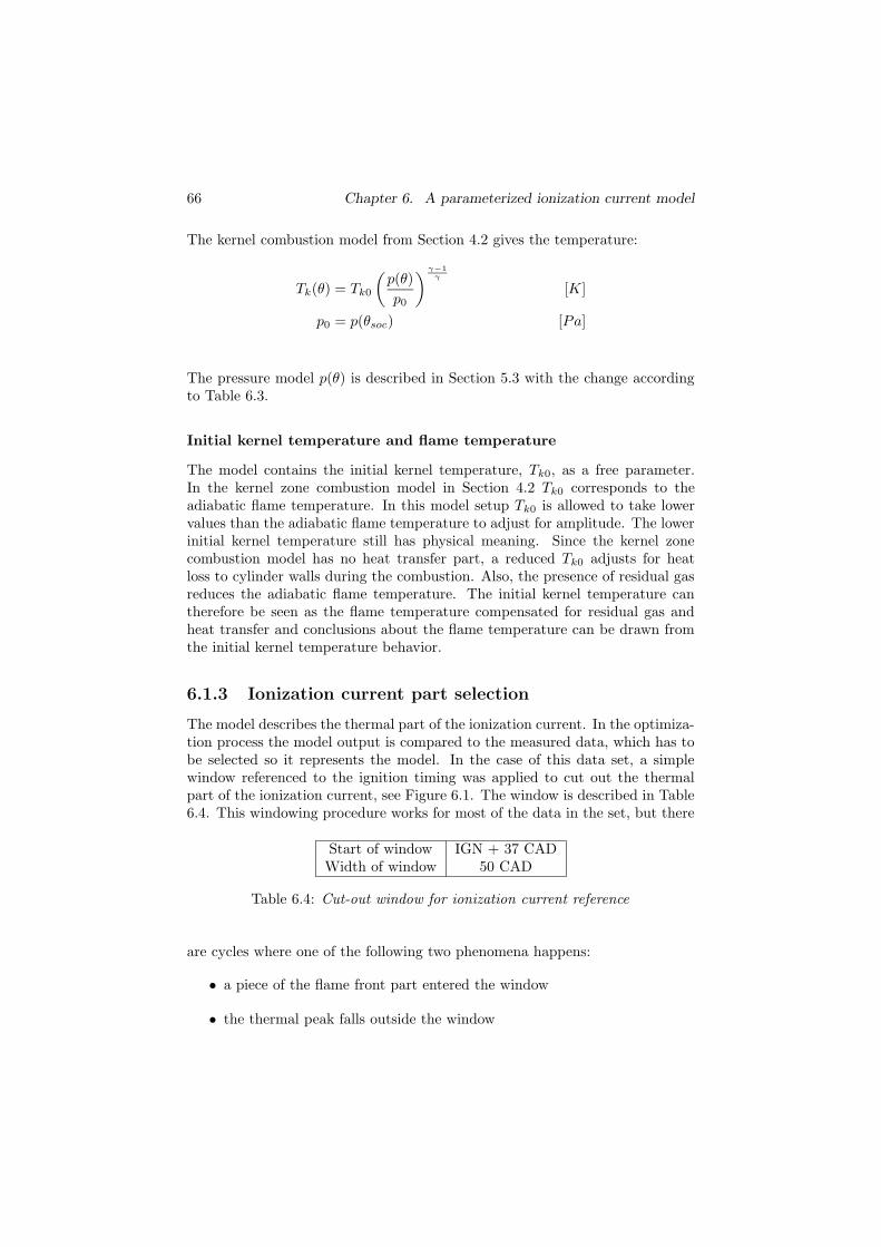
66 Chapter 6. A parameterized ionization current model
The kernel combustion model from Section 4.2 gives the temperature:
Tk(θ) = Tk0
(
p(θ)
p0
)γ−1
γ
[K]
p0 = p(θsoc) [Pa]
The pressure model p(θ) is described in Section 5.3 with the change accordingto Table 6.3.
Initial kernel temperature and flame temperature
The model contains the initial kernel temperature, Tk0, as a free parameter.In the kernel zone combustion model in Section 4.2 Tk0 corresponds to theadiabatic flame temperature. In this model setup Tk0 is allowed to take lowervalues than the adiabatic flame temperature to adjust for amplitude. The lowerinitial kernel temperature still has physical meaning. Since the kernel zonecombustion model has no heat transfer part, a reduced Tk0 adjusts for heatloss to cylinder walls during the combustion. Also, the presence of residual gasreduces the adiabatic flame temperature. The initial kernel temperature cantherefore be seen as the flame temperature compensated for residual gas andheat transfer and conclusions about the flame temperature can be drawn fromthe initial kernel temperature behavior.
6.1.3 Ionization current part selection
The model describes the thermal part of the ionization current. In the optimiza-tion process the model output is compared to the measured data, which has tobe selected so it represents the model. In the case of this data set, a simplewindow referenced to the ignition timing was applied to cut out the thermalpart of the ionization current, see Figure 6.1. The window is described in Table6.4. This windowing procedure works for most of the data in the set, but there
Start of window IGN + 37 CADWidth of window 50 CAD
Table 6.4: Cut-out window for ionization current reference
are cycles where one of the following two phenomena happens:
• a piece of the flame front part entered the window
• the thermal peak falls outside the window
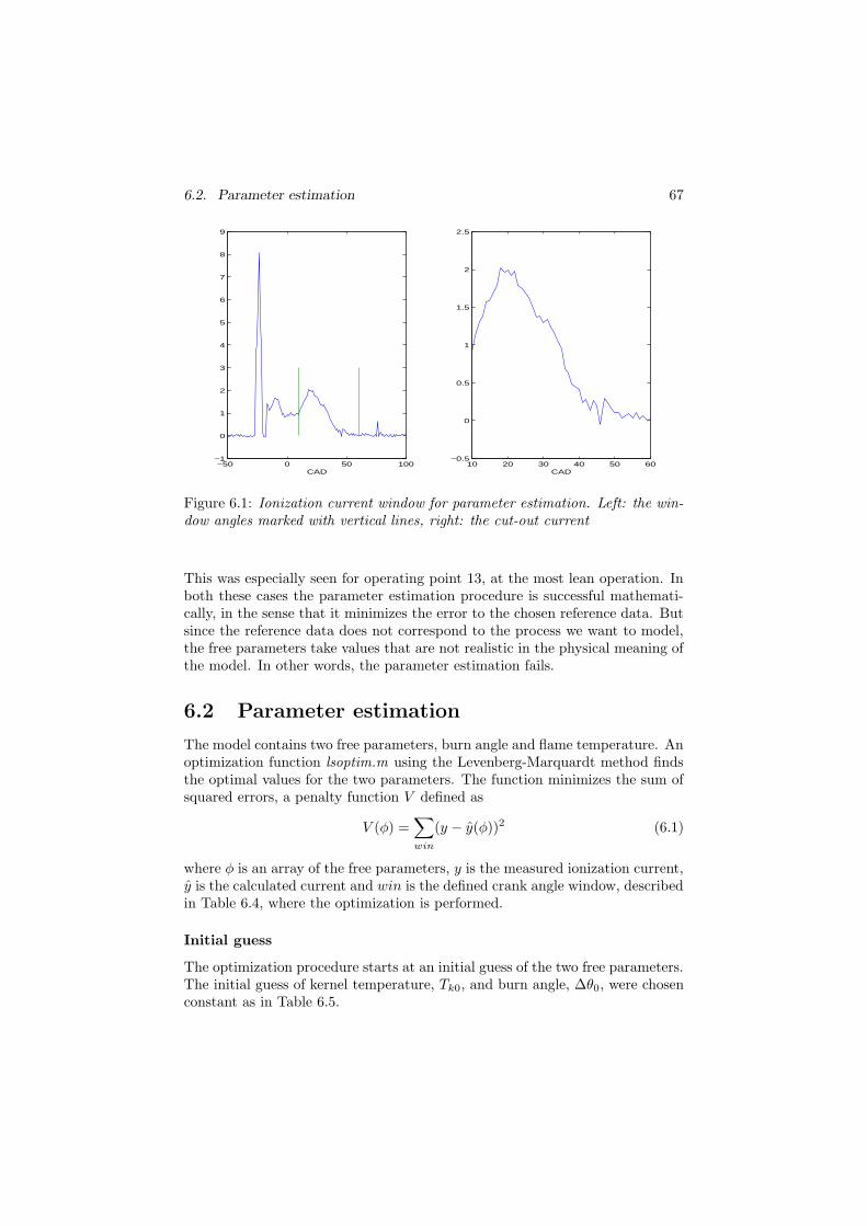
6.2. Parameter estimation 67
−50 0 50 100−1
0
1
2
3
4
5
6
7
8
9
CAD10 20 30 40 50 60
−0.5
0
0.5
1
1.5
2
2.5
CAD
Figure 6.1: Ionization current window for parameter estimation. Left: the win-dow angles marked with vertical lines, right: the cut-out current
This was especially seen for operating point 13, at the most lean operation. Inboth these cases the parameter estimation procedure is successful mathemati-cally, in the sense that it minimizes the error to the chosen reference data. Butsince the reference data does not correspond to the process we want to model,the free parameters take values that are not realistic in the physical meaning ofthe model. In other words, the parameter estimation fails.
6.2 Parameter estimation
The model contains two free parameters, burn angle and flame temperature. Anoptimization function lsoptim.m using the Levenberg-Marquardt method findsthe optimal values for the two parameters. The function minimizes the sum ofsquared errors, a penalty function V defined as
V (φ) =∑
win
(y − y(φ))2 (6.1)
where φ is an array of the free parameters, y is the measured ionization current,y is the calculated current and win is the defined crank angle window, describedin Table 6.4, where the optimization is performed.
Initial guess
The optimization procedure starts at an initial guess of the two free parameters.The initial guess of kernel temperature, Tk0, and burn angle, ∆θ0, were chosenconstant as in Table 6.5.
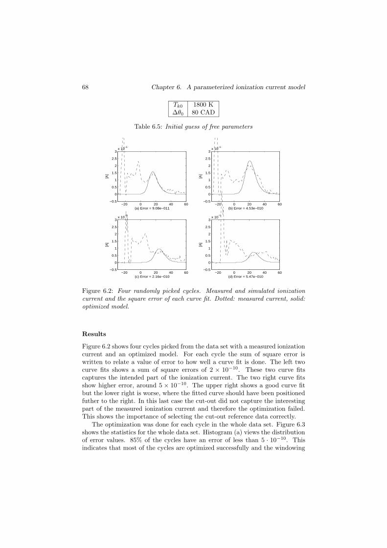
68 Chapter 6. A parameterized ionization current model
Tk0 1800 K∆θ0 80 CAD
Table 6.5: Initial guess of free parameters
−20 0 20 40 60−0.5
0
0.5
1
1.5
2
2.5
3x 10
−5
[A]
(a) Error = 9.08e−011−20 0 20 40 60
−0.5
0
0.5
1
1.5
2
2.5
3x 10
−5
[A]
(b) Error = 4.53e−010
−20 0 20 40 60−0.5
0
0.5
1
1.5
2
2.5
3x 10
−5
[A]
(c) Error = 2.16e−010−20 0 20 40 60
−0.5
0
0.5
1
1.5
2
2.5
3x 10
−5
[A]
(d) Error = 5.47e−010
Figure 6.2: Four randomly picked cycles. Measured and simulated ionizationcurrent and the square error of each curve fit. Dotted: measured current, solid:optimized model.
Results
Figure 6.2 shows four cycles picked from the data set with a measured ionizationcurrent and an optimized model. For each cycle the sum of square error iswritten to relate a value of error to how well a curve fit is done. The left twocurve fits shows a sum of square errors of 2 × 10⁻¹⁰. These two curve fitscaptures the intended part of the ionization current. The two right curve fitsshow higher error, around 5 × 10⁻¹⁰. The upper right shows a good curve fitbut the lower right is worse, where the fitted curve should have been positionedfuther to the right. In this last case the cut-out did not capture the interestingpart of the measured ionization current and therefore the optimization failed.This shows the importance of selecting the cut-out reference data correctly.
The optimization was done for each cycle in the whole data set. Figure 6.3shows the statistics for the whole data set. Histogram (a) views the distributionof error values. 85% of the cycles have an error of less than 5 · 10−10. Thisindicates that most of the cycles are optimized successfully and the windowing
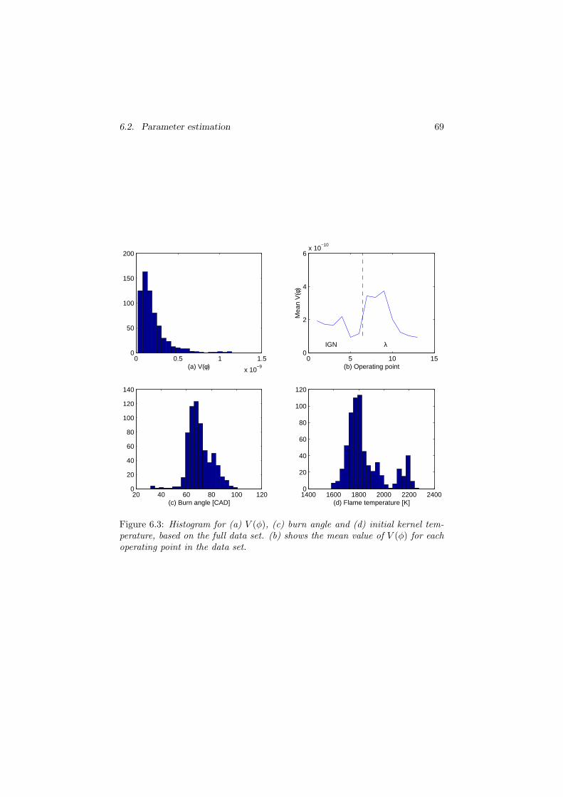
6.2. Parameter estimation 69
0 0.5 1 1.5
x 10−9
0
50
100
150
200
(a) V(φ)0 5 10 15
0
2
4
6x 10
−10
Mea
n V
(φ)
(b) Operating point
IGN λ
20 40 60 80 100 1200
20
40
60
80
100
120
140
(c) Burn angle [CAD]1400 1600 1800 2000 2200 24000
20
40
60
80
100
120
(d) Flame temperature [K]
Figure 6.3: Histogram for (a) V (φ), (c) burn angle and (d) initial kernel tem-perature, based on the full data set. (b) shows the mean value of V (φ) for eachoperating point in the data set.
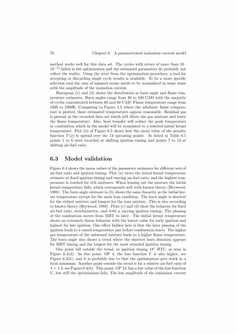
70 Chapter 6. A parameterized ionization current model
method works well for this data set. The cycles with errors of more than 10 ·
10−10 failed in the optimization and the estimated parameters do probably notreflect the reality. Using the error from the optimization procedure, a tool foraccepting or discarding single cycle results is available. To be a more specificselection tool the sum of squared errors needs to be normalized in some sensewith the amplitude of the ionization current.
Histogram (c) and (d) shows the distribution in burn angle and flame tem-perature estimates. Burn angles range from 30 to 100 CAD with the majorityof cycles concentrated between 60 and 80 CAD. Flame temperature range from1600 to 2300K. Comparing to Figure 4.2 where the adiabatic flame tempera-ture is plotted, these estimated temperatures appear reasonable. Residual gasis present in the recorded data set which will dilute the gas mixture and lowerthe flame temperature. Also, heat transfer will reduce the peak temperaturein combustion which in the model will be translated to a lowered initial kerneltemperature. Plot (b) of Figure 6.3 shows how the mean value of the penaltyfunction V (φ) is spread over the 13 operating points. As listed in Table 6.1points 1 to 6 were recorded at shifting ignition timing and points 7 to 13 atshifting air-fuel ratio.
6.3 Model validation
Figure 6.4 shows the mean values of the parameter estimates for different sets ofair-fuel ratio and ignition timing. Plot (a) views the initial kernel temperatureestimate at fixed ignition timing and varying air-fuel ratio, and the highest tem-perature is reached for rich mixtures. When leaning out the mixture the initialkernel temperature falls, which corresponds well with known theory (Heywood,1988). The burn angle estimate in (b) shows the same linearity as the initial ker-nel temperature except for the most lean condition. The burn angle is shortestfor the richest mixture and longest for the lean mixture. This is also accordingto known theory (Heywood, 1988). Plots (c) and (d) show the behavior for fixedair-fuel ratio, stoichiometric, and with a varying ignition timing. The phasingof the combustion moves from MBT to later. The initial kernel temperatureshows an extremely linear behavior with the lowest value for early ignition andhighest for late ignition. One effect hidden here is that the later phasing of theignition leads to a raised temperature just before combustion starts. The highergas temperature of the unburned mixture leads to a higher flame temperature.The burn angle also shows a trend where the shortest burn duration appearsfor MBT timing and the longest for the most retarded ignition timing.
One point fall outside the trend, at ignition timing 18◦ BTC, as seen inFigure 6.4(d). In this point, OP 4, the loss function V is also higher, seeFigure 6.3(b), and it is probably due to that the optimization gets stuck in alocal minimum. Another point outside the trend is for a relative air-fuel ratio ofλ = 1.2, see Figure 6.4(b). This point, OP 13, has a low value of the loss functionV , but still the optimization fails. The low amplitude of the ionization current
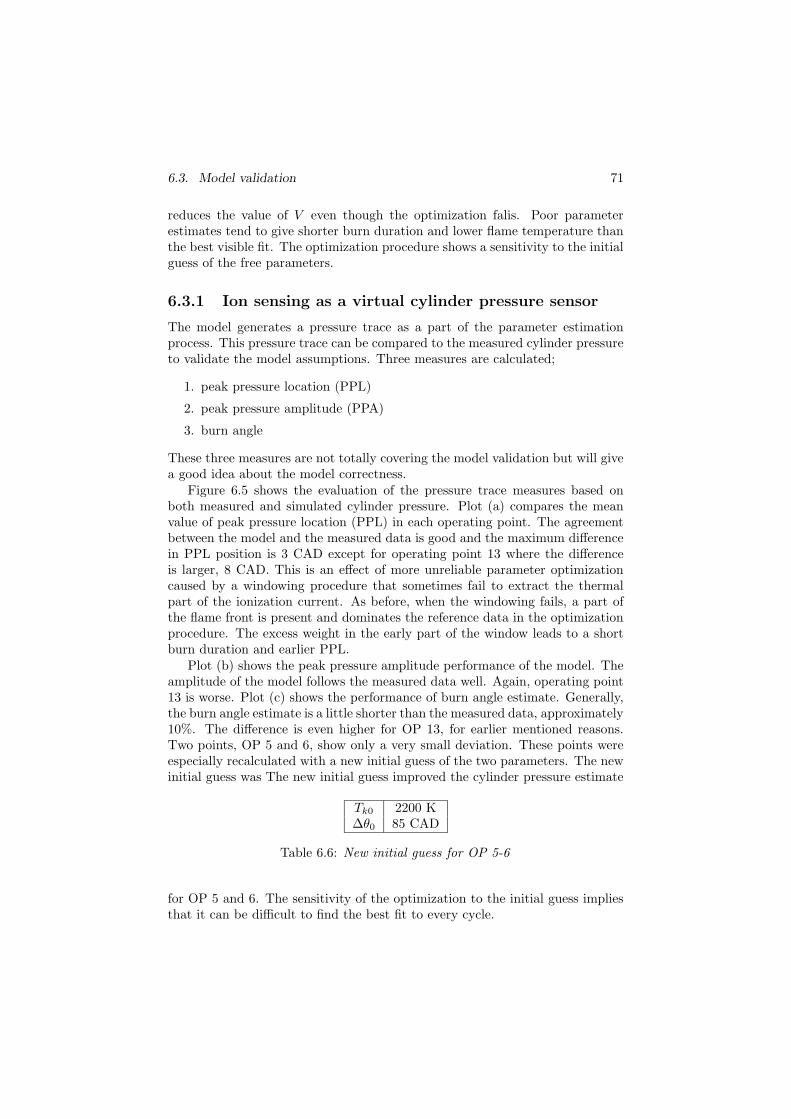
6.3. Model validation 71
reduces the value of V even though the optimization falis. Poor parameterestimates tend to give shorter burn duration and lower flame temperature thanthe best visible fit. The optimization procedure shows a sensitivity to the initialguess of the free parameters.
6.3.1 Ion sensing as a virtual cylinder pressure sensor
The model generates a pressure trace as a part of the parameter estimationprocess. This pressure trace can be compared to the measured cylinder pressureto validate the model assumptions. Three measures are calculated;
1. peak pressure location (PPL)
2. peak pressure amplitude (PPA)
3. burn angle
These three measures are not totally covering the model validation but will givea good idea about the model correctness.
Figure 6.5 shows the evaluation of the pressure trace measures based onboth measured and simulated cylinder pressure. Plot (a) compares the meanvalue of peak pressure location (PPL) in each operating point. The agreementbetween the model and the measured data is good and the maximum differencein PPL position is 3 CAD except for operating point 13 where the differenceis larger, 8 CAD. This is an effect of more unreliable parameter optimizationcaused by a windowing procedure that sometimes fail to extract the thermalpart of the ionization current. As before, when the windowing fails, a part ofthe flame front is present and dominates the reference data in the optimizationprocedure. The excess weight in the early part of the window leads to a shortburn duration and earlier PPL.
Plot (b) shows the peak pressure amplitude performance of the model. Theamplitude of the model follows the measured data well. Again, operating point13 is worse. Plot (c) shows the performance of burn angle estimate. Generally,the burn angle estimate is a little shorter than the measured data, approximately10%. The difference is even higher for OP 13, for earlier mentioned reasons.Two points, OP 5 and 6, show only a very small deviation. These points wereespecially recalculated with a new initial guess of the two parameters. The newinitial guess was The new initial guess improved the cylinder pressure estimate
Tk0 2200 K∆θ0 85 CAD
Table 6.6: New initial guess for OP 5-6
for OP 5 and 6. The sensitivity of the optimization to the initial guess impliesthat it can be difficult to find the best fit to every cycle.
72 Chapter 6. A parameterized ionization current model
0.85 0.9 0.95 1 1.05 1.1 1.15 1.2 1.251680
1700
1720
1740
1760
1780
1800
1820
Lambda
Fla
me
tem
pera
ture
(a) Estimated initial kernel tempera-ture, AFR dependency
0.85 0.9 0.95 1 1.05 1.1 1.15 1.2 1.2563
64
65
66
67
68
69
70
71
72
73
Lambda
Bur
n an
gle
(b) Estimated burn angle, AFR de-pendency
12 14 16 18 20 22 24 26 281750
1800
1850
1900
1950
2000
2050
2100
2150
2200
Ignition angle
Fla
me
tem
pera
ture
(c) Estimated initial kernel tempera-ture, IGN dependency
12 14 16 18 20 22 24 26 2866
68
70
72
74
76
78
80
82
84
Ignition angle
Bur
n an
gle
(d) Estimated burn angle, IGN de-pendency
Figure 6.4: Estimated parameters, initial kernel temperature and burn angle
6.3. Model validation 73
0 2 4 6 8 10 12 1410
15
20
25
30
35
40
Operating point
Mea
n P
PL
[CA
D]
measured simulated
(a) PPL
0 2 4 6 8 10 12 141.6
1.8
2
2.2
2.4
2.6
2.8
3
3.2
3.4
3.6x 10
6
Operating point
Mea
n P
PA
[Pa]
measured simulated
(b) PPA
0 2 4 6 8 10 12 1460
65
70
75
80
85
90
95
100
Operating point
Mea
n bu
rn a
ngle
[CA
D]
measured simulated
(c) Burn angle
Figure 6.5: Comparing pressure trace measures from measured and simulatedcylinder pressure
74 Chapter 6. A parameterized ionization current model
The good agreement between the measured and the simulated pressure dataimplies that the model assumptions made are relevant. The second peak ofthe ionization current can be described by a model for thermal ionization. Theresults also show that the model captures changes in ionization current due tochanged ignition timing and air-fuel ratio.
6.4 Conclusions
A model for the thermal part of the ionization current is composed of four mod-ules; an explicit cylinder pressure model, a kernel zone temperature model, areaction rate controlled NO formation model and a model for thermal ionization.
The model has two free parameters, burn angle and initial kernel tempera-ture. The burn angle affects both position and amplitude of the model outputand the initial kernel temperature affects only the amplitude. This model cap-tures the behavior of the ionization current with respect to amplitude and posi-tion of the thermal part. The free parameters of the model takes values withinphysically motivated ranges. Burn angle varies between 30 and 100 degrees witha peak at 60-80 degrees. Estimated initial kernel temperature range is 1600 to2300 K with a peak at 1800 K. However, it is important to remember thatthese two parameters have to compensate for effects that are not modeled. Oneeffect is heat transfer, that lowers the peak temperature and therefore lowersthe estimated initial kernel temperature in this model.
The model with two free parameters shows good results in calculating thecylinder pressure trace based on optimization to ionization current. The errorof the peak pressure location is less than 3 crank angle degrees and the error ofthe pressure amplitude is less than 20%. This model setup in fact introducesion sensing as a virtual pressure sensor for spark ignited combustion engines.
7
Conclusions
Ion sensing technology has supported engine management systems for the last15 years, providing a channel to monitor the combustion process itself. Overthe years research started to develop physical models for the ionization processto increase the understanding of the underlying physics. One of the modelswas designed by Saitzkoff and Reinmann to explain the second peak of ioniza-tion currents. This ionization model is combined with cylinder pressure andcombustion models and the properties are studied in this thesis.
The thesis includes an investigation of this model in the view of temperatureand nitric oxide dependencies. A first conclusion is that a dynamic model forNO formation is as important as the temperature dependent ionization degreefor the ionization current amplitude for low temperatures, <2400 K, since NOformation in that lower temperature range is a slow reaction. A second resultfrom this investigation is that the volume change in the burned combustionzone is important to consider when calculating NO formation for a combustioncycle. An extension to the NO formation differential equation presented byHeywood is proposed to handle the influence of combustion development andpiston movement on NO concentration.
A model for the second peak of ionization current is presented. The modelconsists of three parts:
• a combustion temperature model
• a reaction rate controlled NO formation model
• a thermal ionization model
with cylinder pressure as input and ionization current as output of the model.
75
76 Chapter 7. Conclusions
An investigation of three different combustion models for temperature showsthat a kernel zone model best supports the thermal ionization idea. The kernelzone model puts the temperature peak, and therefore also the model output ion-ization current peak, closest to the measured ionization current peak. Also, theinitial kernel temperature can be adjusted to fit the model output in amplitudewithout changing the position of the same. The main result from this investi-gation is that thermal ionization can explain the second peak of the ionizationcurrent.
Two major contributions of this thesis are the new cylinder pressure modeland the parameterized ionization current model that includes the new cylinderpressure model.
The cylinder pressure model expresses the cylinder pressure in closed form asa function of crank angle together with measurable inputs and a set of calibra-tion parameters. The calibration parameters all have a physical interpretation.If the burn angles of the combustion are known, this pressure model capturesthe cylinder pressure well.
The cylinder pressure model and the second peak ionization current modelare put together to form the parameterized ionization current model. The modelconsists of four parts:
• a cylinder pressure model
• a combustion temperature model
• a reaction rate controlled NO formation model
• a thermal ionization model
The total model has after calibration two free parameters:
• total burn angle
• initial kernel temperature
The total burn angle is a free parameter in the cylinder pressure part and theinitial kernel temperature appears in the combustion model. Using this modelapproach it is possible to estimate burn angle from a measured ionization cur-rent. With the estimated burn angle and the pressure model a virtual pressuresensor is available, based on ionization current.
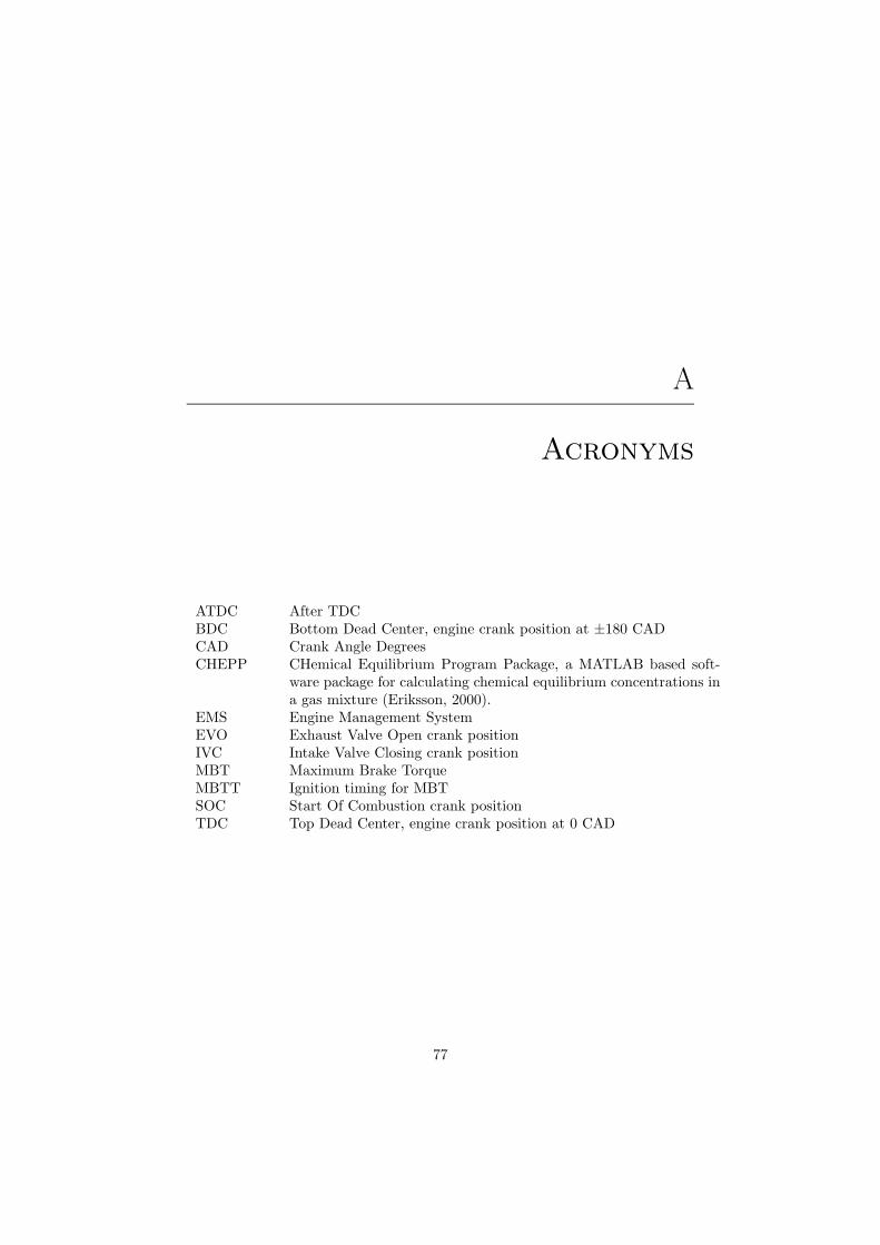
A
Acronyms
ATDC After TDCBDC Bottom Dead Center, engine crank position at ±180 CADCAD Crank Angle DegreesCHEPP CHemical Equilibrium Program Package, a MATLAB based soft-
ware package for calculating chemical equilibrium concentrations ina gas mixture (Eriksson, 2000).
EMS Engine Management SystemEVO Exhaust Valve Open crank positionIVC Intake Valve Closing crank positionMBT Maximum Brake TorqueMBTT Ignition timing for MBTSOC Start Of Combustion crank positionTDC Top Dead Center, engine crank position at 0 CAD
77

78 Appendix A. Acronyms
References
K. Allmendinger, L. Guzzella, and A. Seiler. A method to reduce calculationtime for an internal combustion engine model. SAE Technical Paper no. 2001-mm, (C448/013), 2001.
I. Andersson and L. Eriksson. Ion sensing for combustion stability controlof a spark ignited direct injected engine. Electronic Engine Controls 2000:Controls, (SAE Technical Paper 2000-01-0552), 2000.
M. Asano, T. Kuma, M. Kajitani, and M. Tekeuchi. Development of new ioncurrent combustion control system. SAE paper 980162, 1998.
J. Auzins, H. Johansson, and J. Nytomt. Ion-gap sense in missfire detection,knock and engine control. SAE SP-1082, (SAE paper No. 950004):21–28, 1995.
E. N. Balles, E. A. VanDyne, A. M. Wahl, K. Ratton, and M.-C. Lai. In-cylinder air/fuel ratio approximation using spark gap ionzation sensing. SAEpaper 980166, 1998.
H. F. Calcote. Ion and electron profiles in flames. 9th Symposium (Interna-tional) on Combustion, 1963.
N. Collings, S. Dinsdale, and T. Hands. Plug fouling investigations on a run-ning engine - an application of a novel multi-purpose diagnostic system basedon the spark plug. SAE paper No. 912318, 1991.
P. Csallner. Eine Methode zur Vorasberechnun der Anderun des Brennferlaufesvon Ottomotoren bei geanderten Betriebsbedingungen. PhD thesis, TechnischenUniversitat Munchen, 1980.
79
80 References
C. F. Daniels. The comparison of mass fraction burned obtained from the cylin-der pressure signal and spark plug ion signal. SAE Technical Paper 980140,1998.
L. Eriksson. Requirements for and a systematic method for identifying heat-release model parameters. Modeling of SI and Diesel Engines, SP-1330(SAETechnical Paper no.980626):19–30, 1998.
L. Eriksson. Spark Advance Modeling and Control. PhD thesis, LinkopingUniversity, May 1999. ISBN 91-7219-479-0, ISSN 0345-7524.
L. Eriksson. Documentation for the chemical equilibrium program packagechepp. Technical Report LiTH-R-2298, ISSN 1400-3902, Department of Elec-trical Engineering, Linkoping University, S-581 83 Linkoping, Sweden, 2000.
L. Eriksson, L. Nielsen, and J. Nytomt. Ignition control by ionization currentinterpretation. SAE SP-1149, (SAE paper No. 960045):73–79, 1996.
J. Forster, A. Gunther, M. Ketterer, and K-J. Wald. Ion current sensing forspark ignition engines. SAE 1999-01-0204, 1999.
D. A. Greenhalgh. Gas phase temperature and concentration diagnostics withlasers. SAE Technical Paper 834066, 1983.
M. Hellring, T. Munther, T. Rognvaldsson, N. Wickstrom, C. Carlsson,M. L.son, and J. Nytomt. Robust AFR estimation using the ion current andneural networks. SAE 1999-01-991161, 1999.
J. B. Heywood. Internal Combustion Engine Fundamentals. McGraw-Hillseries in mechanical engineering. McGraw-Hill, 1988.
S.D. Hires, R.J. Tabaczunski, and J.M. Novak. The prediction fo ignition delayand combustion intervals for a homogeneous charge, spark ignition engine. SAETechnical Paper 780232, 1978.
R.B. Krieger and G.L. Borman. The computation of apparent heat release forinternal combustion engines. ASME paper 66-WA/DGP-4, 1966.
G.A Lavoie, J.B.Heywood, and J.C.Keck. Experimental and theoretical studyof nitric oxide formation in internal combustion engines. European Journal ofControl, 1, 1970.
A. Lee and J. S. Pyko. Engine misfire detection by ionization current moni-toring. SAE SP-1082, (SAE paper No. 950003):9–19, 1995.
F. A. Matekunas. Modes and measures of cyclic combustion variability. SAETechnical Paper 830337, 1983.
References 81
F. A. Matekunas. Spark ignition engines – combustion characteristics, ther-modynamics, and the cylinder pressure card. Central States Section, TheCombustion Institute, March 19-20 1984. Minneapolis, Mn.
F. A. Matekunas. Engine combustion control with ignition timing by pressureratio management. US Pat., A, 4622939, Nov. 18 1986.
M. Mladek and L. Guzzella. A model for the estimation of residual gas fractionusing cylinder pressure measurements. SAE Technical Paper 2000-01-0958,2000.
L. Nielsen and L. Eriksson. An ion-sense engine-fine-tuner. IEEE ControlSystems (special issue on powertrain control), Vol. 18(5):43–52, October 1998.
Y. Nilsson and L. Eriksson. A new formulation of multi-zone combustion enginemodels. pages 379–387, Karlsruhe, Germany, 2001, 2001. Elsevier Science. 3rdIFAC Workshop ”Advances in Automotive Control”, Preprints.
R. Reinmann. Theoretical and Experimental Studies of the Formation of Ion-ized Gases in Spark Ignited Engines. PhD thesis, Lund Institute of Technology,April 1998. ISBN 91-628-2985-8, ISSN 1102-8718.
R. Reinmann, A. Saitzkoff, B. Lassesson, and P. Strandh. Fuel and additiveinfluend on the ion current. SAE Technical Paper 980161, 1998.
R. Reinmann, A. Saitzkoff, F. Mauss, and M. Glavmo. Local air-fuel ratiomeasurements using the spark plug as an ionization sensor. SAE paper No.970856, (SAE SP-1263):175–185, 1997.
A. Saitzkoff, R. Reinmann, T. Berglind, and M. Glavmo. An ionization equi-librium analysis of the spark plug as an ionization sensor. SAE paper No.960337, 1996.
A. Saitzkoff, R. Reinmann, and F. Mauss. In cylinder pressure measurementsusing the spark plug as an ionization sensor. SAE paper No. 970857, pages187–197, 1997.
Y. Shimasaki, M. Kanehiro, S. Baba, S. Maruyama, T. Hisaki, and S. Miy-ata. Spark plug voltage analysis for monitoring combustion in an internalcombustion engine. SAE paper No. 930461, 1993.
I.I. Vibe. Brennverlauf und Kreisprocess von Verbennungsmotoren. VEB Ver-lag Technik Berlin, 1970. German translation of the russian original.
H. Wilstermann. Wechselspannungszundung mit integrierter Ionenstrommes-sung als Sensor fur die Verbrennungs- und Motorregelung. PhD thesis, Uni-versity Fridericiana of Karlsruhe, April 1999. ISBN 3-18-338912-6, ISSN 0178-9449.

82 Notes
S. Yoshiyama, E. Tomita, and Y. Hamamoto. Fundamental study on combus-tion diagnostics using a spark plug as ion probe. SAE 2000-01-2828, 2000.
Ya.B. Zeldovich, P.Ya. Sadovnikov, and D.A. Frank-Kamenetskii. Oxidationof nitrogen in combustion. Technical report, Academy of Sciences of USSR, In-stitute of Chemical Physics Moscow-Leningrad, 1947. Translated by M.Shelef1970, Ford Motor Company.

Notes 83

84 Notes

Notes 85