cyme 5-02-basic analyses user guide en v1-2
TRANSCRIPT

January 2011
CYME 5.02
CYMDIST Basic Analyses Users Guide

© Copyright CYME International T&D Inc.
All Rights Reserved No part of this publication may be reproduced, or transmitted in any form
or by any means without the written permission of CYME International T&D. Possession or use of the CYME software described in this publication is
authorized only pursuant to a valid written license agreement from CYME. CYME makes no warranty, either expressed or implied, including but not
limited to any implied warranties of merchantability or fitness for a particular purpose, regarding these materials and makes such materials available solely on an "as-is" basis.
CYME International T&D reserves the right to revise and improve its products as it sees fit. The information in this manual is subject to modification without notice.
While every precaution has been taken in the preparation of this manual, CYME assumes no responsibility for errors or omissions, or for damages resulting from the use of the information contained herein.
CYME International T&D Inc.
1485 Roberval, Suite 104 St-Bruno QC J3V 3P8
Canada
Tel.: (450) 461-3655 Fax: (450) 461-0966
Canada & United States: Tel.:1-800-361-3627 Internet : http://www.cyme.com
E-mail: [email protected] Other Trademarks: The names of all products and services other than CYME’s
mentioned in this document are the trademarks or trade names of the respective owners.


CYME 5.02 – CYMDIST Basic Analyses – Users Guide
TABLE OF CONTENTS 1
Table of Contents
Chapter 1 Load Flow Analysis ....................................................................................1 1.1 Introduction ...................................................................................................1 1.2 Parameters Tab ............................................................................................2
1.2.1 Calculation Methods.........................................................................3 1.2.2 Convergence Parameters ................................................................3 1.2.3 Calculation Options ..........................................................................3 1.2.4 Load and Generation Scaling Factors..............................................4 1.2.5 Voltage and Frequency Sensitivity Load Model...............................8
1.3 Calculation Methods ...................................................................................13 1.3.1 Voltage Drop Calculation Technique..............................................13 1.3.2 Gauss-Seidel..................................................................................14 1.3.3 Newton-Raphson............................................................................15 1.3.4 Fast-Decoupled ..............................................................................16
1.4 Networks Tab..............................................................................................17 1.5 Controls Tab ...............................................................................................18 1.6 Loading / Voltage Limits Tab ......................................................................19 1.7 Output Tab..................................................................................................21 1.8 Solving the Load Flow ................................................................................23 1.9 Results ........................................................................................................25
1.9.1 Reports ...........................................................................................25 1.9.2 Report by Individual Section...........................................................27 1.9.3 Charts .............................................................................................29 1.9.4 One-Line Diagram Tags.................................................................30 1.9.5 One-Line Diagram Coloring ...........................................................31
1.10 Convergence Issues...................................................................................32 1.10.1 Voltage Drop Method .....................................................................32 1.10.2 Gauss-Seidel, Fast Decoupled and Newton-Raphson Methods ...33 1.10.3 Networks with Abnormal Voltages .................................................34 1.10.4 Parallel Operation of Generators ...................................................35
Chapter 2 Short-Circuit Analysis..............................................................................37 2.1 Conventional Short-Circuit Analysis ...........................................................38
2.1.1 Fault Parameters Tab.....................................................................39 2.1.2 Networks Tab .................................................................................44 2.1.3 Output tab.......................................................................................45
2.2 ANSI Short-Circuit Analysis........................................................................46 2.2.1 ANSI Parameters Tab ....................................................................47 2.2.2 Networks Tab .................................................................................50 2.2.3 Output Tab......................................................................................51
2.3 IEC Short-Circuit Analysis ..........................................................................52 2.3.1 IEC Parameters Tab.......................................................................53 2.3.2 Networks Tab .................................................................................58 2.3.3 Output Tab......................................................................................59
2.4 Results ........................................................................................................60 2.4.1 Reports ...........................................................................................60 2.4.2 Report by Individual Section...........................................................61 2.4.3 Charts .............................................................................................63 2.4.4 Report Tags....................................................................................64 2.4.5 One-Line Diagram Coloring ...........................................................64
Chapter 3 Fault Analysis ...........................................................................................65

CYME 5.02 – CYMDIST Basic Analyses – Users Guide
2 TABLE OF CONTENTS
3.1 Shunt Fault Analysis ...................................................................................65 3.1.1 Parameters Tab..............................................................................66 3.1.2 Output Tab......................................................................................68 3.1.3 Shunt Fault Results ........................................................................69
3.2 Network Fault Analysis ...............................................................................70 3.2.1 Parameters Tab..............................................................................70 3.2.2 Results............................................................................................71
3.3 Voltage Sag Analysis..................................................................................73 3.3.1 Parameters Tab..............................................................................73 3.3.2 Results............................................................................................74
3.4 Fault Locator Analysis ................................................................................75 3.4.1 Parameters Tab..............................................................................76 3.4.2 Results............................................................................................77
Chapter 4 Motor Starting Analysis ...........................................................................79 4.1 Locked Rotor Motor Start Analysis .............................................................79
4.1.1 List of Motors and Parameters .......................................................79 4.1.2 Flicker Table...................................................................................80 4.1.3 Locked Rotor Starting Assistance Methods ...................................82 4.1.4 Running and Viewing the Results of a Locked Rotor Analysis ......82 4.1.5 Locked Rotor Analysis Sample Output ..........................................83 4.1.6 Display: Color by Voltage Dip ........................................................84
4.2 Maximum Start Size Analysis .....................................................................85 4.2.1 Running the Analysis and Viewing the Results..............................85
Chapter 5 Load Allocation.........................................................................................87 5.1.1 Summary of the Connected kVA Method.......................................92 5.1.2 Summary of the kWH Method ........................................................93 5.1.3 Summary of Actual kVA Method ....................................................93 5.1.4 Summary of the REA Method.........................................................93
Chapter 6 Load Balancing Calculation ....................................................................97 6.1.1 Location Tab...................................................................................98 6.1.2 Display Tab...................................................................................100 6.1.3 Result Tab ....................................................................................101 6.1.4 Load Balancing Report.................................................................102
Chapter 7 Capacitor Placement Calculation .........................................................105 7.1 Objectives Tab..........................................................................................105 7.2 Restrictions Tab........................................................................................106 7.3 Capacitor Banks Tab ................................................................................107 7.4 Load Levels Tab .......................................................................................109 7.5 Results Tab...............................................................................................110 7.6 Iterative Search.........................................................................................112
7.6.1 Iterative Search Results ...............................................................112 7.6.2 Iterative Search Color Coding ......................................................114

CYME 5.02 – CYMDIST Basic Analyses – Users Guide
CHAPTER 1 – LOAD FLOW ANALYSIS 1
Chapter 1 Load Flow Analysis
1.1 Introduction
The objective of a load flow is to analyze the steady-state performance of the power system under various operating conditions. It is the basic analysis tool for the planning, design and operation of any electrical power systems. These could be distribution, industrial or transmission networks.
The basic load flow question for a known power system configuration is a follows: Given:
• the load power consumption at all buses • the power production at each generator
Find:
• the voltage magnitude and phase angle at each bus • the power flow through each line and transformer
The CYME Load Flow module provides the user with solution algorithms for both balanced and unbalanced networks.
For Unbalanced networks, the Voltage Drop calculation method based on current iterations is used as the solution algorithm. The Unbalanced module requires CYMDIST.
For Balanced networks, the user has the choice of the following calculation methods:
• Voltage Drop (Requires CYMDIST)
• Fast Decoupled (Requires CYMFLOW)
• Full Newton-Raphson (Requires CYMFLOW)
• Gauss-Seidel (Requires CYMFLOW)
CYME 5.02 – CYMDIST Basic Analyses – Users Guide
2 CHAPTER 1 – LOAD FLOW ANALYSIS
1.2 Parameters Tab
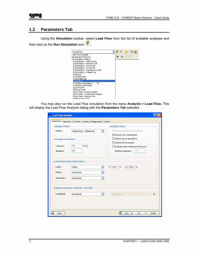
Using the Simulation toolbar, select Load Flow from the list of available analyses and
then click on the Run Simulation icon .
You may also run the Load Flow simulation from the menu Analysis > Load Flow. This will display the Load Flow Analysis dialog with the Parameters Tab selected.
CYME 5.02 – CYMDIST Basic Analyses – Users Guide
CHAPTER 1 – LOAD FLOW ANALYSIS 3
1.2.1 Calculation Methods
Method Select the load flow calculation method from the list of available methods:
• Voltage Drop - Unbalanced & Balanced • Fast Decoupled - Balanced • Gauss-Seidel - Balanced • Newton-Raphson – Balanced
Refer to 1.3 Calculation Methods for a detailed description of the load flow methods.
1.2.2 Convergence Parameters
Tolerance If the mismatch between two successive iterations is within the specified tolerance then the load flow will declare convergence of the network. The % voltage deviation (dV) is the convergence criteria for the Voltage drop methods. All the other methods use the power mismatch as the convergence criteria.
Iterations Limits the total number of iterations to a pre-defined number. The number of iterations can be increased if the program does not converge.
As an example the Fast-Decoupled method will normally converge within 10-20 iterations. Gauss-Seidel may require much more iterations.
1.2.3 Calculation Options
Flat Start (At Nominal Conditions)
Check this option to initialize all Voltages to the system nominal voltages (usually 1.0 p.u.) prior to the first load flow iteration. All Capacitors, Tap Changers, Regulators and Generators will also be initialized to their initial states as defined in the network settings. If you do not check this option, the states and voltages of the previous load flow will be re-submitted as initial conditions for the load flow calculation.
Assume Line Transposition
When performing an Unbalanced Load Flow, you have the option to assume or not line transposition in the calculation of the overhead line impedance matrix. This option has an effect on the calculation only when the overhead lines are modeled By-Phase with a valid phase position.
Include Source Impedance
Include source impedance in the load flow calculation. This option will be automatically active in the locked rotor analysis where voltage dips may prevent voltage regulation at substation terminals.
Remove All Constraints
If this option is checked then the load flow will be solved by relaxing all the constraints on Generators (Qmax and Qmin), Load Tap Changing Transformers and Regulators. Note: This is useful for networks that have difficulty converging since
the results of the load flow, with relaxed constraints, can provide useful tips as to where the problem may be.

CYME 5.02 – CYMDIST Basic Analyses – Users Guide
4 CHAPTER 1 – LOAD FLOW ANALYSIS
Evaluate State of Network Protectors
This option concerns networks with Network Protectors, which are usually installed inside Secondary Networks. Should this option be selected, then the analysis would take into consideration the fact that Network Protectors would open if backward flow is detected. Users can set a number of Maximum attempts within which the analysis will try to find a solution for the final state of the network protectors for the configuration of the network under study.
1.2.4 Load and Generation Scaling Factors
Scaling factors can be globally applied to Loads, Motors and Generators without the need to edit the network settings. Four different methods are offered to apply the scaling factors:
• As Defined • Global • By Zone • By Equipment Type (Load, Generator or Motor)
By default the factors will be set to “As Defined” and implies that no scaling factors will be applied to any of the equipment.
Global factors apply to all Loads, Motors or Generators in the network. The factor for each data entry field implies that the actual value of (P, Q ) as entered in the network settings or database will be multiplied by the Factor/100%. For the power factor, the values defined in the network settings will be replaced by the global power factor for the purpose of the simulation.
By Zone implies that the factors will apply on specified zones of the network.

CYME 5.02 – CYMDIST Basic Analyses – Users Guide
CHAPTER 1 – LOAD FLOW ANALYSIS 5
By default, all factors are set to 100 %. To Edit the default values or to Create a new set
of factors click on the icon. For loads, for example, the Load Scaling Factors (by Zone) dialog box with a listing of all zones defined in the network and the default P and Q values will be displayed on screen.
Click on the icon to create a new set of user defined scaling factors to be applied on the respective zones. A dialog will prompt you for a name. Enter the desired name (ex: Light Load).
When creating a new set of factors, you have the option to initialize the values using default values (Use default values) or to copy existing values from another template (Use values from).

CYME 5.02 – CYMDIST Basic Analyses – Users Guide
6 CHAPTER 1 – LOAD FLOW ANALYSIS
To delete a user defined set of factors click on the icon. The same applies to Generators (P, Qmin, Qmax) and Motors (P, PF).
By Load/Motor/Generator Type implies that the factors will apply on the specified equipments only.
Click on the icon to edit the factors. For Loads for example, this option multiplies all Active (P) and Reactive (Q) loads separately based on their customer type assignments. Type in the factors in the spaces provided. For example: Setting the active load factor (P) = 110 % implies that the load entered in the Load Properties dialog box will be multiplied by 1.1 (10% increase). Check the option P=Q if you wish to enter the same values for the active and reactive power
You can create any number of templates (set of factors). For example, a set of factors could represent a specific period (time of day, season, peak etc) or a specific study mode (Planning, Design, etc). To select a template, click on the symbol and select the desired name.
For Motors, scaling factors can be applied to Induction and Synchronous Motors separately.
CYME 5.02 – CYMDIST Basic Analyses – Users Guide
CHAPTER 1 – LOAD FLOW ANALYSIS 7
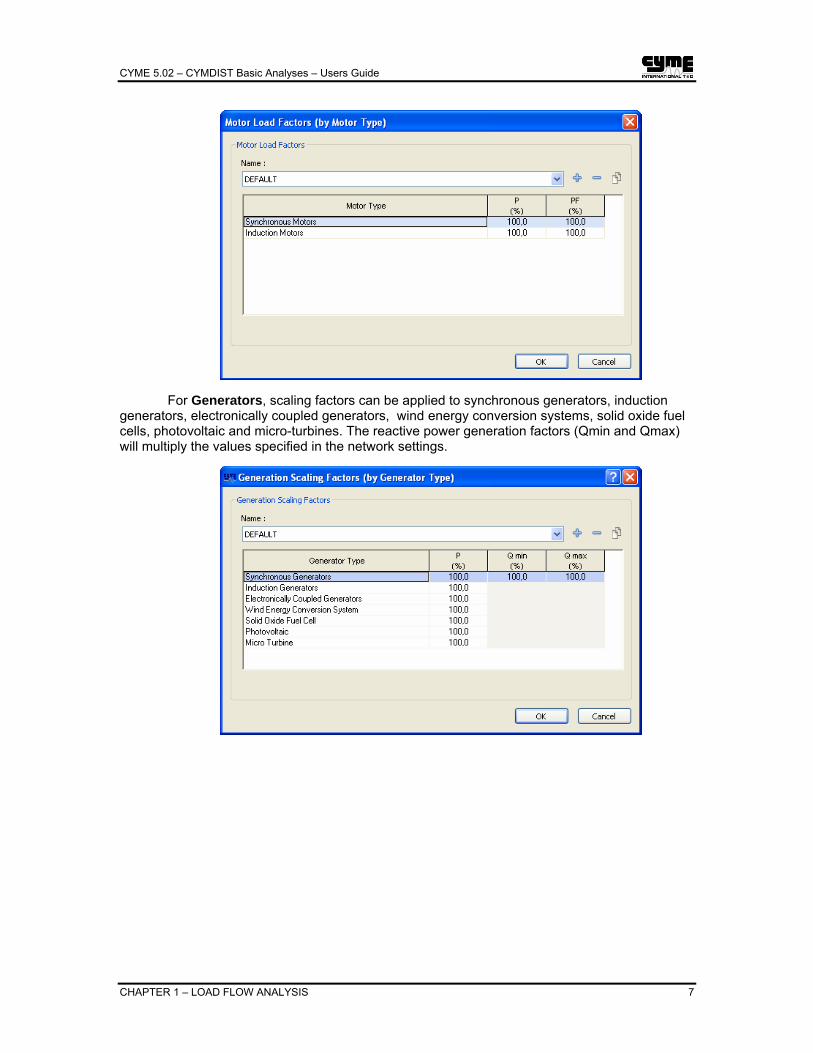
For Generators, scaling factors can be applied to synchronous generators, induction generators, electronically coupled generators, wind energy conversion systems, solid oxide fuel cells, photovoltaic and micro-turbines. The reactive power generation factors (Qmin and Qmax) will multiply the values specified in the network settings.
CYME 5.02 – CYMDIST Basic Analyses – Users Guide
8 CHAPTER 1 – LOAD FLOW ANALYSIS
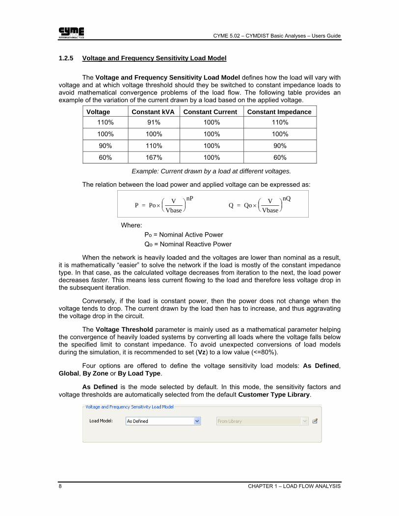
1.2.5 Voltage and Frequency Sensitivity Load Model
The Voltage and Frequency Sensitivity Load Model defines how the load will vary with voltage and at which voltage threshold should they be switched to constant impedance loads to avoid mathematical convergence problems of the load flow. The following table provides an example of the variation of the current drawn by a load based on the applied voltage.
Voltage Constant kVA Constant Current Constant Impedance 110% 91% 100% 110%
100% 100% 100% 100%
90% 110% 100% 90%
60% 167% 100% 60%
Example: Current drawn by a load at different voltages.
The relation between the load power and applied voltage can be expressed as:
P = PonPV
Vbase× ⎛⎝⎜
⎞⎠⎟
Q = QonQV
Vbase× ⎛⎝⎜
⎞⎠⎟
Where: Po = Nominal Active Power Qo = Nominal Reactive Power
When the network is heavily loaded and the voltages are lower than nominal as a result, it is mathematically “easier” to solve the network if the load is mostly of the constant impedance type. In that case, as the calculated voltage decreases from iteration to the next, the load power decreases faster. This means less current flowing to the load and therefore less voltage drop in the subsequent iteration.
Conversely, if the load is constant power, then the power does not change when the voltage tends to drop. The current drawn by the load then has to increase, and thus aggravating the voltage drop in the circuit.
The Voltage Threshold parameter is mainly used as a mathematical parameter helping the convergence of heavily loaded systems by converting all loads where the voltage falls below the specified limit to constant impedance. To avoid unexpected conversions of load models during the simulation, it is recommended to set (Vz) to a low value (<=80%).
Four options are offered to define the voltage sensitivity load models: As Defined, Global, By Zone or By Load Type.
As Defined is the mode selected by default. In this mode, the sensitivity factors and voltage thresholds are automatically selected from the default Customer Type Library.

CYME 5.02 – CYMDIST Basic Analyses – Users Guide
CHAPTER 1 – LOAD FLOW ANALYSIS 9
Click on the icon to view or modify the default values of the customer type library. The Customer Type Library is part of the network settings. For more information on creating new Customer Types and/or editing the default library values, refer to chapters on Network Types and Customer Types (Network menu) in the CYME Reference Manual.
Global allows you to apply the same exponent sensitivity factors (nP, nQ) and voltage threshold (Vz) to all loads in the network. The exponent sensitivity factors must be specified in p.u. and the voltage threshold in %.
By Zone implies that the exponent factors and voltage threshold will apply to all the loads of the selected zones.
To “Edit” the default values or “Create” a new set of factors click on the icon.
Note: If you have the optional Transient Stability Analysis module, additional entries will be available in this group box to specify the Frequency Sensitivity factors. Refer to the Transient Analysis User Guide for further information.
CYME 5.02 – CYMDIST Basic Analyses – Users Guide
10 CHAPTER 1 – LOAD FLOW ANALYSIS
Note: The above dialog box implies the following: • All loads in Zone L1 will be constant power loads. • All loads in Zone L2 will be constant impedance loads. • The voltage threshold in Zones L1 and L2 is set to 80 %.
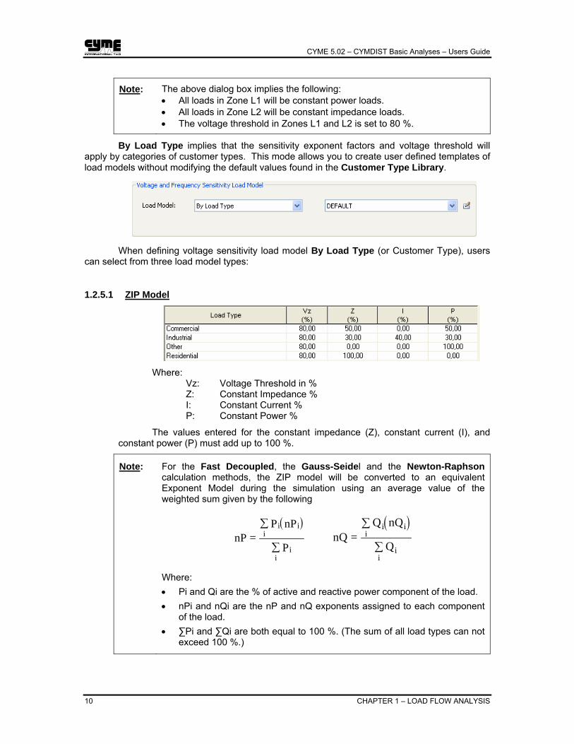
By Load Type implies that the sensitivity exponent factors and voltage threshold will apply by categories of customer types. This mode allows you to create user defined templates of load models without modifying the default values found in the Customer Type Library.
When defining voltage sensitivity load model By Load Type (or Customer Type), users can select from three load model types:
1.2.5.1 ZIP Model
Where: Vz: Voltage Threshold in % Z: Constant Impedance % I: Constant Current % P: Constant Power %
The values entered for the constant impedance (Z), constant current (I), and constant power (P) must add up to 100 %.
Note: For the Fast Decoupled, the Gauss-Seidel and the Newton-Raphson calculation methods, the ZIP model will be converted to an equivalent Exponent Model during the simulation using an average value of the weighted sum given by the following
( )nP
P nP
P
ii
i
ii
=∑
∑
( )nQ =
Q nQ
Q
ii
i
ii
∑
∑
Where: • Pi and Qi are the % of active and reactive power component of the load. • nPi and nQi are the nP and nQ exponents assigned to each component
of the load. • ∑Pi and ∑Qi are both equal to 100 %. (The sum of all load types can not
exceed 100 %.)

CYME 5.02 – CYMDIST Basic Analyses – Users Guide
CHAPTER 1 – LOAD FLOW ANALYSIS 11
As an example, the following composite load model was created:
Then the average nP or nQ value are computed as follows:
nP or nQ = (50 % x 0.0) + (30 % x 1) + (20 % x 2) = 0 + 0.3 + 0.4 = 0.70 100%
Those values will be used in the Load Flow Analysis for the calculation methods mentioned above. If you connect a non-rotating load and an induction motor on the same bus, then the load will have nP = nQ = 0, regardless of the values you specify.
1.2.5.2 Exponent Model
Where:
Vz: Voltage Threshold in %
nP: Active Power Exponent factor in p.u.
nQ: Reactive Power Exponent factor in p.u.
Note: • nP or nQ = 0.0 means constant-power load
• nP or nQ = 1.0 means constant-current load
• nP or nQ = 2.0 means constant-impedance load
1.2.5.3 Mixed: ZIP and Exponent Model
By default, the values will be initialized to the values found in the study file
parameters (if working with an older study) or the default values from the Customer Type Library otherwise.

CYME 5.02 – CYMDIST Basic Analyses – Users Guide
12 CHAPTER 1 – LOAD FLOW ANALYSIS
To create a new Voltage Sensitivity Load Model click on the icon to create a new set of user defined voltage sensitivity and threshold factors. The following dialog will be displayed:
Name Enter the name for the particular Voltage Sensitivity Load Model.
Type Select the Voltage Sensitivity Load Model Type: Zip, Exponent or Mixed.
Blank Initialize all data entry fields as blank. From Copy the values from another voltage sensitivity load model From Default Values
Copy the values from the default Customer Type Library

CYME 5.02 – CYMDIST Basic Analyses – Users Guide
CHAPTER 1 – LOAD FLOW ANALYSIS 13
1.3 Calculation Methods
1.3.1 Voltage Drop Calculation Technique
The Load Flow analysis of a radial distribution feeder requires an iterative technique that is specifically designed and optimized for radial or weakly meshed systems. The Voltage Drop Analysis method includes a full three phase unbalanced algorithm that computes phase voltages (VA, VB and VC), power flows and currents including the neutral current.
The iterative Voltage Drop calculation technique will compute the voltages and power flows at every section within 10 or less iterations. The calculation returns the results when no calculated voltage on any section of the selected networks changes from one iteration to the next by more than the Calculation tolerance. Example: |34465.2 – 34464.8|/34464.8 < 0.1%.
However, in some cases, the calculation may not converge to a solution which could either be due to bad data such as a very high impedance line or could be due to peculiar network configuration.
If during the calculation process the voltage on a section falls below the specified Voltage Threshold, then for the next iteration, all loads on that section will be converted to constant impedances.
Converting the load in this way does not affect the load data permanently. It is only a way to assist the calculation to converge to a “solution”, instead of not giving any result at all.
You can use this (artificial) solution to identify problem areas or sections with bad input data, by looking for section(s) with very low voltage. To avoid using this function, set the voltage threshold to a low value, such as <=80%. Setting the level higher than 90% is not recommended, for fear of distorting an otherwise valid solution.
When you select to run a Balanced Voltage Drop the calculation will be performed with the load on every section assumed to be distributed equally among all the available phases. This will not change the load data that you have entered through the Section Properties dialog box.
CYME 5.02 – CYMDIST Basic Analyses – Users Guide
14 CHAPTER 1 – LOAD FLOW ANALYSIS
1.3.2 Gauss-Seidel
Transmission network power flow analysis techniques are specifically designed for balanced three phase systems and may exhibit poor convergence characteristics when applied to radial distribution type feeders.
The set of system equations are typically non-linear, and solving them does require the use of iterative algorithms.
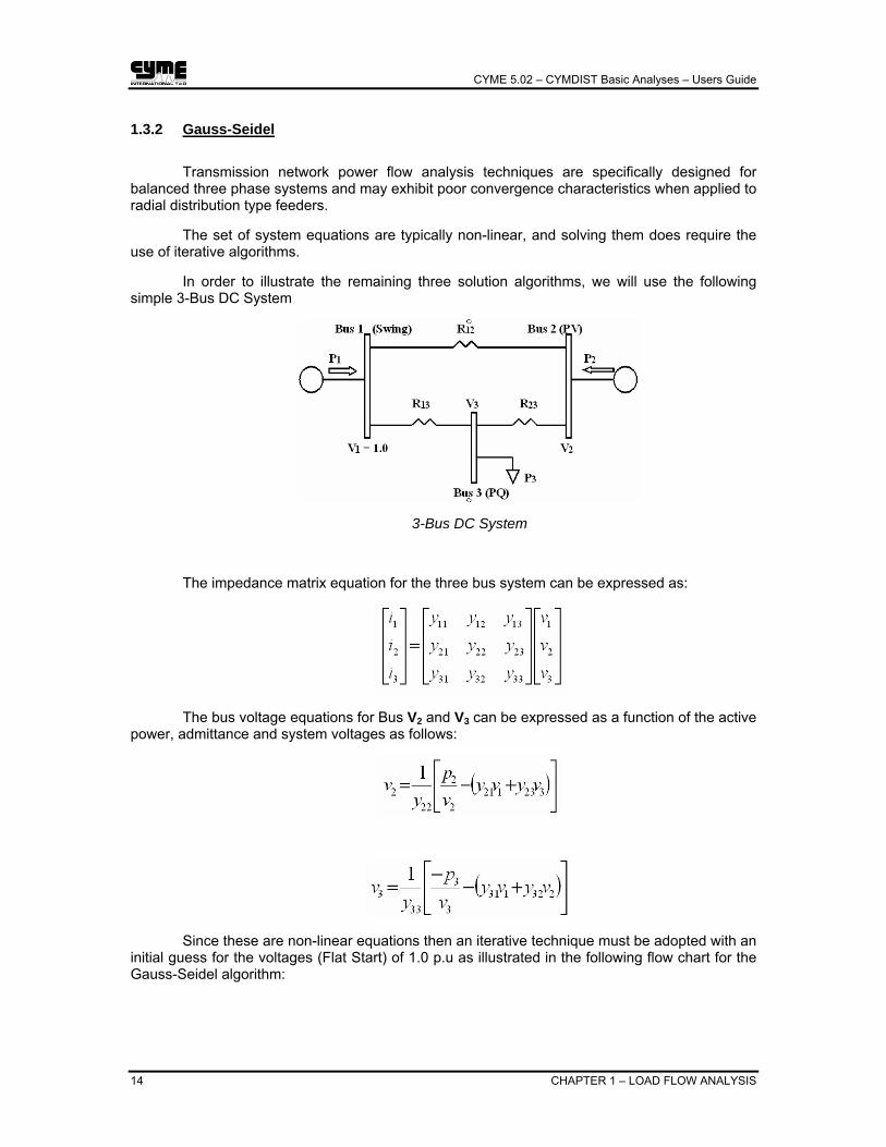
In order to illustrate the remaining three solution algorithms, we will use the following simple 3-Bus DC System
3-Bus DC System
The impedance matrix equation for the three bus system can be expressed as:
The bus voltage equations for Bus V2 and V3 can be expressed as a function of the active power, admittance and system voltages as follows:
Since these are non-linear equations then an iterative technique must be adopted with an initial guess for the voltages (Flat Start) of 1.0 p.u as illustrated in the following flow chart for the Gauss-Seidel algorithm:

CYME 5.02 – CYMDIST Basic Analyses – Users Guide
CHAPTER 1 – LOAD FLOW ANALYSIS 15
Hint: The Gauss-Seidel method may offer better chances for convergence in networks with significant resistance in them. (Branches with X/R < 1.0). Note that this method normally requires a greater number of iterations to converge to the solution than the other solution methods.
1.3.3 Newton-Raphson
The Newton-Raphson method of solving the power-flow problem is an iterative algorithm for solving a set of simultaneous non-linear equations and an equal number of unknowns based on the Taylor’s series expansion for a function of two or more variables.
The power equations at each bus will be as follows:
The derivative term is a follows:
CYME 5.02 – CYMDIST Basic Analyses – Users Guide
16 CHAPTER 1 – LOAD FLOW ANALYSIS
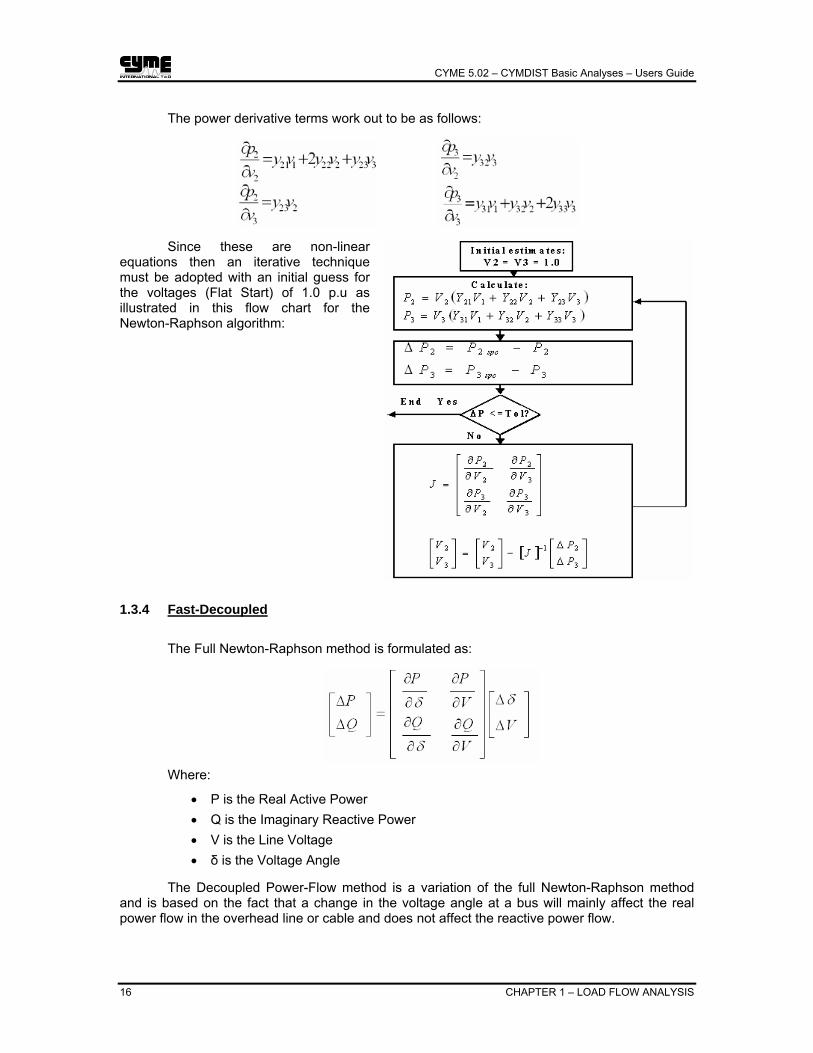
The power derivative terms work out to be as follows:
Since these are non-linear equations then an iterative technique must be adopted with an initial guess for the voltages (Flat Start) of 1.0 p.u as illustrated in this flow chart for the Newton-Raphson algorithm:
1.3.4 Fast-Decoupled
The Full Newton-Raphson method is formulated as:
Where:
• P is the Real Active Power • Q is the Imaginary Reactive Power • V is the Line Voltage • δ is the Voltage Angle
The Decoupled Power-Flow method is a variation of the full Newton-Raphson method and is based on the fact that a change in the voltage angle at a bus will mainly affect the real power flow in the overhead line or cable and does not affect the reactive power flow.

CYME 5.02 – CYMDIST Basic Analyses – Users Guide
CHAPTER 1 – LOAD FLOW ANALYSIS 17
Similarly, a change in the voltage magnitude will have a direct impact on the reactive power flow and does affect the active power flow.
With this in mind the following derivative terms can be approximately set to zero.
The active and reactive power derivative terms can be approximated by the following simplified equations:
The iterative technique of the Fast-Decoupled method is the same as the Newton-Raphson method.
1.4 Networks Tab
Select in the list the networks you wish to analyze. Click on the check box next to a network name to select or de-select it individually. Click on the symbol to expand the list and on to collapse it again. All selects every feeder loaded in the study. None de-selects all feeders.

CYME 5.02 – CYMDIST Basic Analyses – Users Guide
18 CHAPTER 1 – LOAD FLOW ANALYSIS
Note: The Load Flow module can simultaneously solve multiple networks and networks with multiple swing buses.
1.5 Controls Tab
The modifications made in this dialog do not permanently change the status of capacitors, regulators, transformers, generators and motors as defined in then network settings. Rather, it simply allows you take them in and out of service for a particular analysis.
If the check box next to the item is unchecked then they are ignored (Off) for the analysis as they are considered temporarily disconnected, even if their individual status indicates that they are in service.
Take for example a capacitor that is controlled by the voltage at its terminals. Whether it is initially “On” or “Off”, it will be considered as disconnected and will never turn on if Capacitors: Voltage Control option is unchecked in this dialog box.
Note: This is the only way to turn on/off time-controlled capacitors without changing their status individually.
Hint: “Fixed capacitor” will behave as “manual control”.
CYME 5.02 – CYMDIST Basic Analyses – Users Guide
CHAPTER 1 – LOAD FLOW ANALYSIS 19
For Regulator and Transformer Tap Operation, the following analysis options are available:
Normal Tap Operation
The Normal Tap Operation setting uses the taps as defined in the Network Settings.
Infinite Taps The Infinite Tap option does not consider any step; the regulated voltage will then be exactly the desired voltage.
Hint: During the planning stage, you can select Infinite Taps to ensure you get the exact desired voltage.
Lock Taps at their Specified Positions
If this option is checked then the load flow is solved by fixing the tap position of all Regulators and Load Tap Changing Transformers to the initial tap position as defined in the network settings.
Disable Tap Changer
This option has the same effect as setting the tap changer to its neutral position (no voltage adjustment).
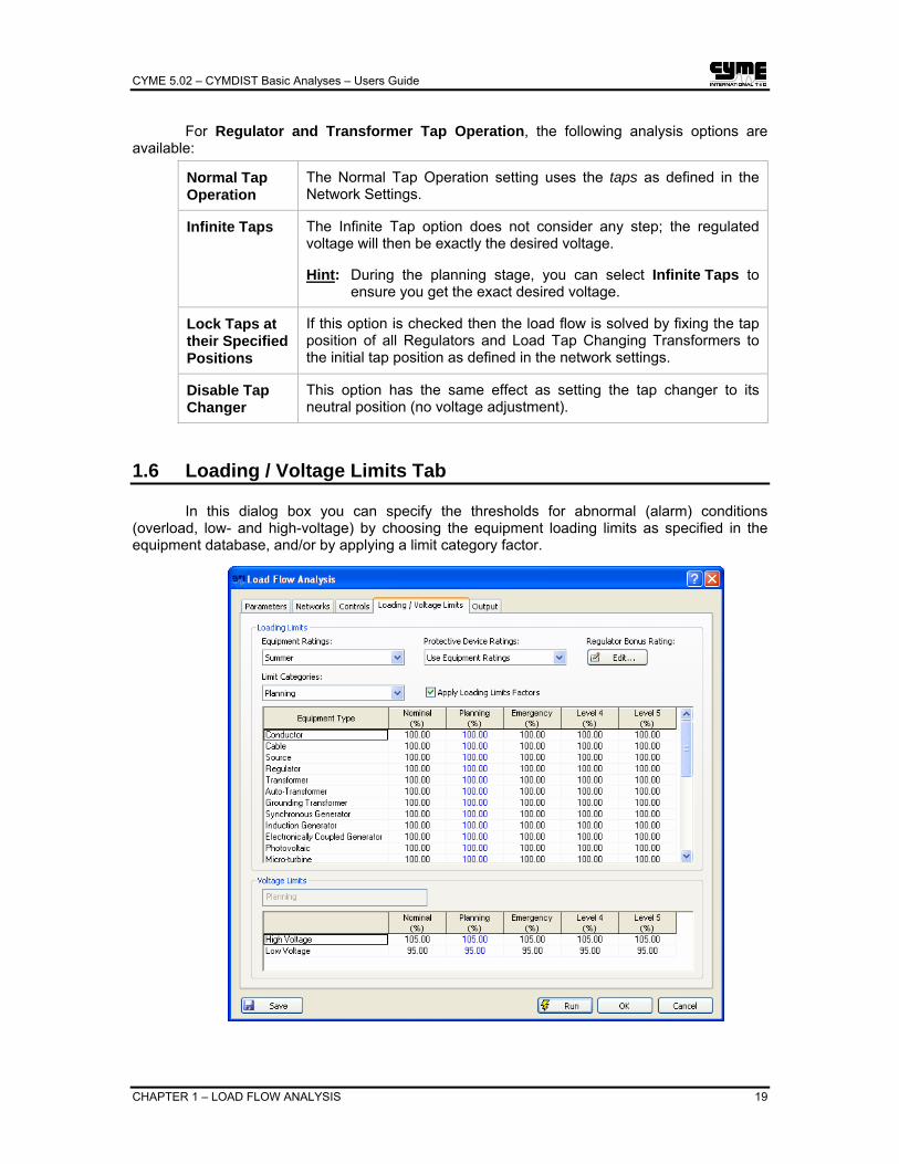
1.6 Loading / Voltage Limits Tab
In this dialog box you can specify the thresholds for abnormal (alarm) conditions (overload, low- and high-voltage) by choosing the equipment loading limits as specified in the equipment database, and/or by applying a limit category factor.
CYME 5.02 – CYMDIST Basic Analyses – Users Guide
20 CHAPTER 1 – LOAD FLOW ANALYSIS
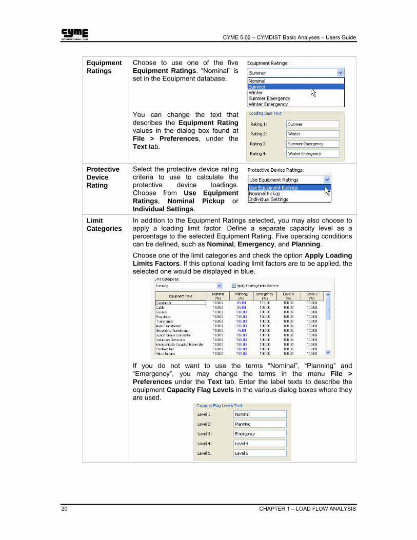
Choose to use one of the five Equipment Ratings. “Nominal” is set in the Equipment database.
Equipment Ratings
You can change the text that describes the Equipment Rating values in the dialog box found at File > Preferences, under the Text tab.
Protective Device Rating
Select the protective device rating criteria to use to calculate the protective device loadings. Choose from Use Equipment Ratings, Nominal Pickup or Individual Settings.
Limit Categories
In addition to the Equipment Ratings selected, you may also choose to apply a loading limit factor. Define a separate capacity level as a percentage to the selected Equipment Rating. Five operating conditions can be defined, such as Nominal, Emergency, and Planning. Choose one of the limit categories and check the option Apply Loading Limits Factors. If this optional loading limit factors are to be applied, the selected one would be displayed in blue.
If you do not want to use the terms “Nominal”, “Planning” and “Emergency”, you may change the terms in the menu File > Preferences under the Text tab. Enter the label texts to describe the equipment Capacity Flag Levels in the various dialog boxes where they are used.
CYME 5.02 – CYMDIST Basic Analyses – Users Guide
CHAPTER 1 – LOAD FLOW ANALYSIS 21
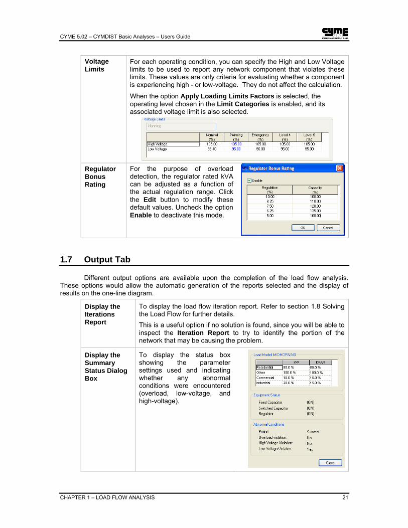
Voltage Limits
For each operating condition, you can specify the High and Low Voltage limits to be used to report any network component that violates these limits. These values are only criteria for evaluating whether a component is experiencing high - or low-voltage. They do not affect the calculation.
When the option Apply Loading Limits Factors is selected, the operating level chosen in the Limit Categories is enabled, and its associated voltage limit is also selected.
Regulator Bonus Rating
For the purpose of overload detection, the regulator rated kVA can be adjusted as a function of the actual regulation range. Click the Edit button to modify these default values. Uncheck the option Enable to deactivate this mode.
1.7 Output Tab
Different output options are available upon the completion of the load flow analysis. These options would allow the automatic generation of the reports selected and the display of results on the one-line diagram.
Display the Iterations Report
To display the load flow iteration report. Refer to section 1.8 Solving the Load Flow for further details. This is a useful option if no solution is found, since you will be able to inspect the Iteration Report to try to identify the portion of the network that may be causing the problem.
Display the Summary Status Dialog Box
To display the status box showing the parameter settings used and indicating whether any abnormal conditions were encountered (overload, low-voltage, and high-voltage).
CYME 5.02 – CYMDIST Basic Analyses – Users Guide
22 CHAPTER 1 – LOAD FLOW ANALYSIS
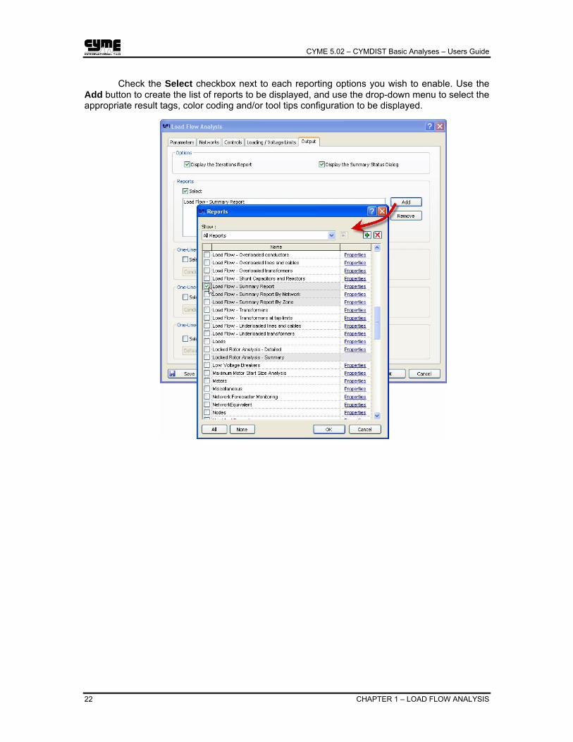
Check the Select checkbox next to each reporting options you wish to enable. Use the Add button to create the list of reports to be displayed, and use the drop-down menu to select the appropriate result tags, color coding and/or tool tips configuration to be displayed.

CYME 5.02 – CYMDIST Basic Analyses – Users Guide
CHAPTER 1 – LOAD FLOW ANALYSIS 23
1.8 Solving the Load Flow
Once the parameters for the load flow analysis have been set, you may click on the Save button if you wish to permanently save the parameters to your disk. This is only useful if you wish to re-use the same parameters as default parameters for future studies.
Click on the Run button to start the analysis. Depending on the calculation method selected, the following iteration reports will be displayed (if the option Display Iteration Report is checked).
For the Voltage Drop calculation methods, the following report will be displayed.
At each iteration, the load flow computes the voltage at every section in the network. It compares the new values with the values it calculated from the previous iteration and reports the section where the voltage has changed the most (Max dV in %). The process continues until the solution is found or until the maximum number of iterations is reached.
For the Fast Decoupled, the Newton-Raphson and the Gauss-Seidel calculation methods, the following iteration report will be displayed.
The convergence criteria for these methods is power dP (Active Power) and dQ (Reactive Power) in respect to the calculation tolerance specified in the calculation parameters.

CYME 5.02 – CYMDIST Basic Analyses – Users Guide
24 CHAPTER 1 – LOAD FLOW ANALYSIS
Mismatches Are the differences between specified and calculated power at a bus. At every iteration the software returns the largest mismatch and the affected bus. dP and dQ are respectively the largest active power and reactive power mismatches. Both are expressed in per-unit of the MVA base (not in MW and MVAR directly).
(Example: dP = .7743E-01 means 0.07743 x 100 MVA = 7.743 MW.)
Bus is the bus where the corresponding mismatch (dP or dQ) occurs. Examine that part of the network if the calculation does not converge.
Adjustments Lists two numbers in each of seven columns, in the form N / M. This means that N devices of that type have been set to their limits in the present iteration, and that M devices might otherwise have exceeded their limits:
Area Means the specified active power (MW) flow from one area to another cannot be satisfied and that the flow has been set to the maximum possible.
Gen Means the reactive power limit of a generator(s) has been reached.
TCV Means the tap of a Voltage Regulating transformer has reached one of its limits.
TCQ Means the tap of a Reactive Power Regulating transformer has reached one of its limits.
TCP Means that the tap of a Phase-shifting transformer has reached one of its limits.
DCL Means that one of the converter angles has reached its limit in a HVDC Line.
SwG Means that the maximum VAR adjustment of a switchable shunt has been reached.
Hints: • You might inspect this report to see whether devices are continually being adjusted.
• If so, try changing the settings of one or more of them before solving again.

CYME 5.02 – CYMDIST Basic Analyses – Users Guide
CHAPTER 1 – LOAD FLOW ANALYSIS 25
1.9 Results
1.9.1 Reports
To select and display the load flow reports click on the icon of the Simulation toolbar or select Report > On Calculation from the menu.
.
Here are a few samples of reports that can be selected.
Sample Load Flow Summary Report

CYME 5.02 – CYMDIST Basic Analyses – Users Guide
26 CHAPTER 1 – LOAD FLOW ANALYSIS
Notes on the Load Flow Summary report:
1. Differences between Load Read (non-adjusted) and Load Used: a. Load Read: Total load connected to the network, i.e., the sum of
each individual load point. b. Load Used: Total load used for the Load Flow analysis. This value
may be different from the load as it is influenced by the load scaling factors, the voltage sensitivity load model and the constant impedance voltage threshold.
2. Annual Cost of System Losses: CYME first annualizes the kW losses calculated through the Load Flow analysis considering the load factor defined for each network (Edit > Add Network > Demand tab, Annual Losses group box). Then, the Cost of energy defined under the report’s Properties is used to calculate the total annual cost.
Sample Load Flow Feeder Loading Report
CYME 5.02 – CYMDIST Basic Analyses – Users Guide
CHAPTER 1 – LOAD FLOW ANALYSIS 27
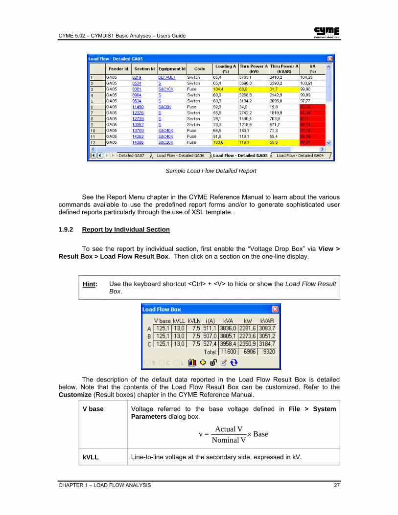
Sample Load Flow Detailed Report
See the Report Menu chapter in the CYME Reference Manual to learn about the various commands available to use the predefined report forms and/or to generate sophisticated user defined reports particularly through the use of XSL template.
1.9.2 Report by Individual Section
To see the report by individual section, first enable the “Voltage Drop Box” via View > Result Box > Load Flow Result Box. Then click on a section on the one-line display.
Hint: Use the keyboard shortcut <Ctrl> + <V> to hide or show the Load Flow Result Box.
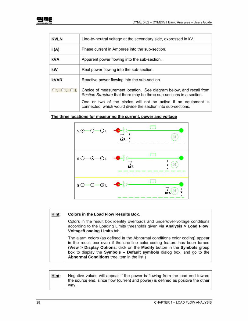
The description of the default data reported in the Load Flow Result Box is detailed below. Note that the contents of the Load Flow Result Box can be customized. Refer to the Customize (Result boxes) chapter in the CYME Reference Manual.
V base Voltage referred to the base voltage defined in File > System Parameters dialog box.
BaseVNominal
V Actual=v ×
kVLL Line-to-line voltage at the secondary side, expressed in kV.
CYME 5.02 – CYMDIST Basic Analyses – Users Guide
28 CHAPTER 1 – LOAD FLOW ANALYSIS
KVLN Line-to-neutral voltage at the secondary side, expressed in kV.
i (A) Phase current in Amperes into the sub-section.
kVA Apparent power flowing into the sub-section.
kW Real power flowing into the sub-section.
kVAR Reactive power flowing into the sub-section.
Choice of measurement location. See diagram below, and recall from Section Structure that there may be three sub-sections in a section.
One or two of the circles will not be active if no equipment is connected, which would divide the section into sub-sections.
The three locations for measuring the current, power and voltage
Hint: Colors in the Load Flow Results Box.
Colors in the result box identify overloads and under/over-voltage conditions according to the Loading Limits thresholds given via Analysis > Load Flow, Voltage/Loading Limits tab.
The alarm colors (as defined in the Abnormal conditions color coding) appear in the result box even if the one-line color-coding feature has been turned (View > Display Options; click on the Modify button in the Symbols group box to display the Symbols – Default symbols dialog box, and go to the Abnormal Conditions tree item in the list.)
Hint: Negative values will appear if the power is flowing from the load end toward the source end, since flow (current and power) is defined as positive the other way.
CYME 5.02 – CYMDIST Basic Analyses – Users Guide
CHAPTER 1 – LOAD FLOW ANALYSIS 29
Click on the button to display the Chart Selection dialog box. Refer to section 1.9.3 Charts, for further details.
The last four buttons of the Result box ( ) will help monitor multiple locations. See the Customize Menu chapter of the CYME Reference Manual, under Result Boxes.
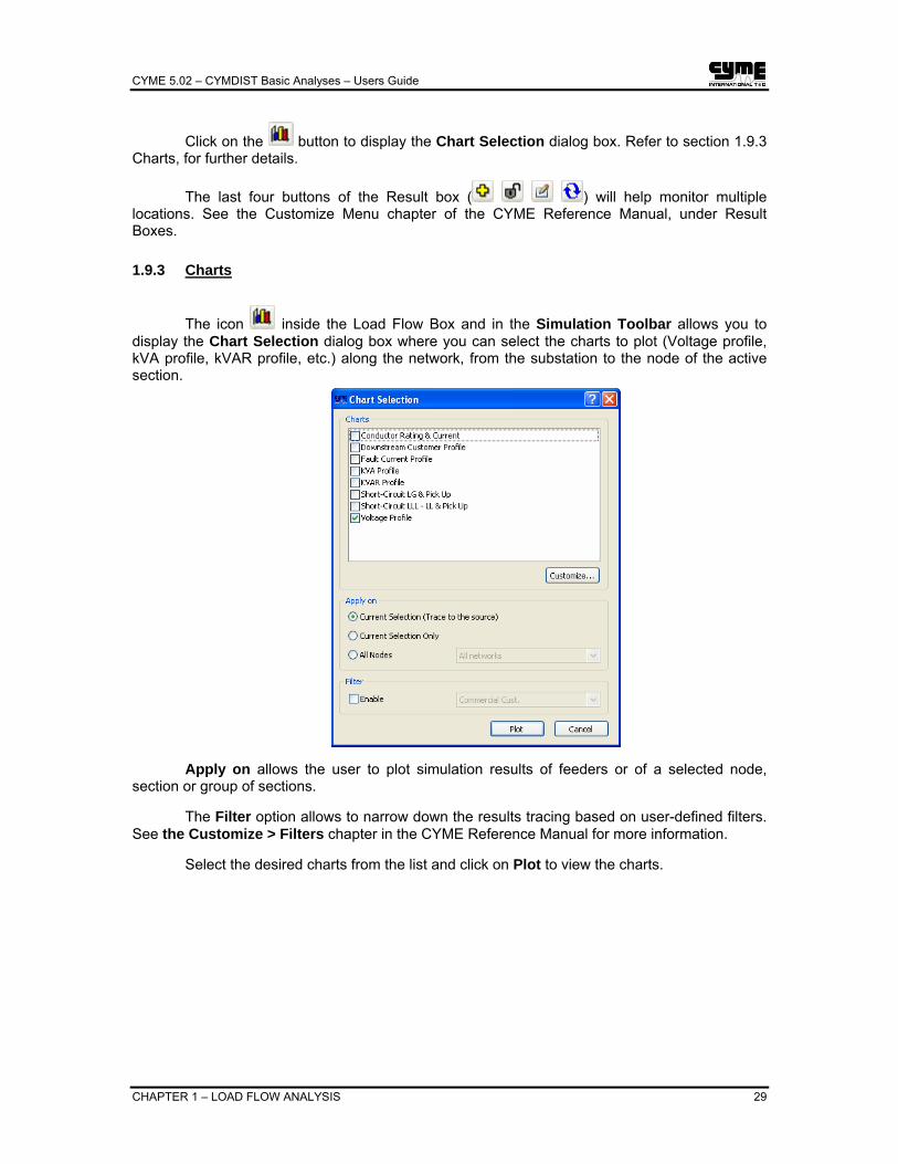
1.9.3 Charts
The icon inside the Load Flow Box and in the Simulation Toolbar allows you to display the Chart Selection dialog box where you can select the charts to plot (Voltage profile, kVA profile, kVAR profile, etc.) along the network, from the substation to the node of the active section.
Apply on allows the user to plot simulation results of feeders or of a selected node, section or group of sections.
The Filter option allows to narrow down the results tracing based on user-defined filters. See the Customize > Filters chapter in the CYME Reference Manual for more information.
Select the desired charts from the list and click on Plot to view the charts.
CYME 5.02 – CYMDIST Basic Analyses – Users Guide
30 CHAPTER 1 – LOAD FLOW ANALYSIS
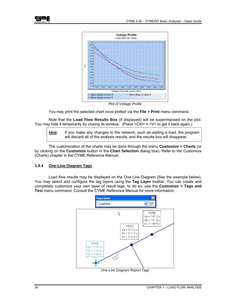
Plot of Voltage Profile
You may print the selected chart once plotted via the File > Print menu command.
Note that the Load Flow Results Box (if displayed) will be superimposed on the plot. You may hide it temporarily by closing its window. (Press <Ctrl> + <V> to get it back again.)
Hint: If you make any changes to the network, such as adding a load, the program will discard all of the analysis results, and the results box will disappear.
The customization of the charts may be done through the menu Customize > Charts (or by clicking on the Customize button in the Chart Selection dialog box). Refer to the Customize (Charts) chapter in the CYME Reference Manual.
1.9.4 One-Line Diagram Tags
Load flow results may be displayed on the One Line Diagram (See the example below). You may select and configure the tag layers using the Tag Layer toolbar. You can create and completely customize your own layer of result tags; to do so, use the Customize > Tags and Text menu command. Consult the CYME Reference Manual for more information.
One-Line Diagram Report Tags

CYME 5.02 – CYMDIST Basic Analyses – Users Guide
CHAPTER 1 – LOAD FLOW ANALYSIS 31
Hint: The Tool Tip can also be used to display the Tag contents. Hovering your mouse over a section will display the tool tip. The contents of the tool tip can be modified. To do so, go to the Tool tips group box of the View > Display Options dialog box.
1.9.5 One-Line Diagram Coloring
The one-line diagram can be color-coded based on the load flow results. You can select from a list of predefined coloring layers or you can create your own color coding layer. You may select the active color coding layer using the Color Coding Layer toolbar. You can create and completely customize your own color coding; to do so, use the Customize > Color coding menu command. Consult the CYME Reference Manual for more information.

CYME 5.02 – CYMDIST Basic Analyses – Users Guide
32 CHAPTER 1 – LOAD FLOW ANALYSIS
Refer to the Display Options chapter in the CYME Reference Manual to learn how to customize and create new one-line diagram color coding layer.
You may also display the abnormal conditions on the one-line diagram by clicking on the
icon of the analysis toolbar.
.
1.10 Convergence Issues
Some networks may exhibit difficulty in converging or do not converge at all. This chapter provides you some hints as to what you need to look for.
1.10.1 Voltage Drop Method
When the Voltage Drop calculation method fails to converge, the following recommended steps should help you find the potential causes of the non-convergence.
1. Enable the option Display the Iterations Report in the Load flow parameters tab.
2. Try relaxing the constraints on the devices by enabling the option Remove All Constraints in the Load flow parameters tab. If the Load flow converges, investigate the setting adjustments of regulators, LTCs and generators.
3. Try reducing the load factor until the load flow converges. For example, try a load factor of 70% (global load factor =70%) and continue to reduce the load factor until the Load flow does converge. Once you have a solution, identify the areas with low voltages and investigate those areas for potentially large loads or large impedances.
4. If you see that the Max dV is increasing steadily in the iteration report, check the input data for components connected to the indicated section. Look for very high impedance.
Hints: • Check that transformer voltages are entered in kV, not Volts.For example, 480 V is 0.48 kV, not 480 kV.
• Make sure line and cable lengths are consistent with the unit of length specified
• For example 15000 ft. is 2.84 mi, not 15000 mi.
5. If you see that the Max dV steadily decreases in the iteration report but remains higher than the specified solution tolerance when the permitted number of iterations is exhausted, try increasing the number of iterations before solving again. See Analysis > Load Flow, Parameters Tab.
6. If you see that the Max dV becomes large and repeatedly increases and then decreases in the iteration report look for a very high load downstream supplied through a large impedance.
CYME 5.02 – CYMDIST Basic Analyses – Users Guide
CHAPTER 1 – LOAD FLOW ANALYSIS 33
7. Verify the settings of switched capacitors, regulators, LTC transformers, and generators. Make sure that the control settings are adequate.
Hint: A Cancel button allows you to cancel the calculation before all of the permitted iterations are performed, in case the calculation is not converging. Use it to save you some time.
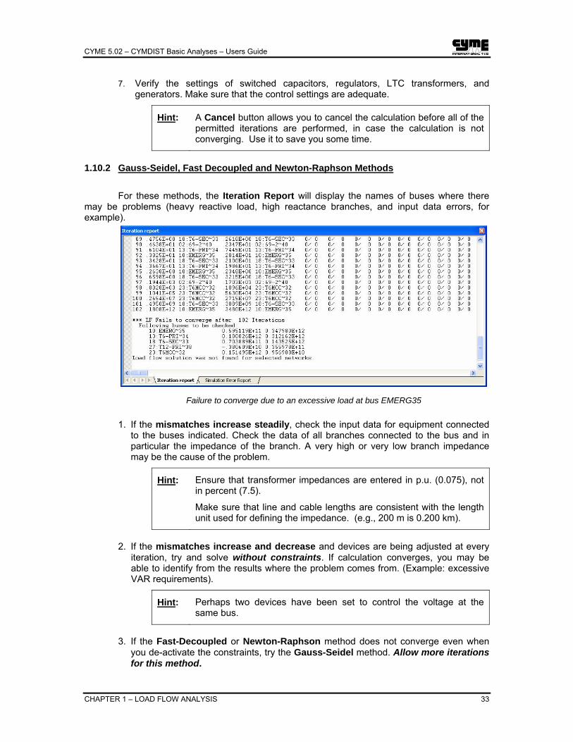
1.10.2 Gauss-Seidel, Fast Decoupled and Newton-Raphson Methods
For these methods, the Iteration Report will display the names of buses where there may be problems (heavy reactive load, high reactance branches, and input data errors, for example).
Failure to converge due to an excessive load at bus EMERG35 1. If the mismatches increase steadily, check the input data for equipment connected
to the buses indicated. Check the data of all branches connected to the bus and in particular the impedance of the branch. A very high or very low branch impedance may be the cause of the problem.
Hint: Ensure that transformer impedances are entered in p.u. (0.075), not in percent (7.5).
Make sure that line and cable lengths are consistent with the length unit used for defining the impedance. (e.g., 200 m is 0.200 km).
2. If the mismatches increase and decrease and devices are being adjusted at every
iteration, try and solve without constraints. If calculation converges, you may be able to identify from the results where the problem comes from. (Example: excessive VAR requirements).
Hint: Perhaps two devices have been set to control the voltage at the same bus.
3. If the Fast-Decoupled or Newton-Raphson method does not converge even when
you de-activate the constraints, try the Gauss-Seidel method. Allow more iterations for this method.
CYME 5.02 – CYMDIST Basic Analyses – Users Guide
34 CHAPTER 1 – LOAD FLOW ANALYSIS
4. If the mismatches steadily decrease but remain higher than the specified solution tolerance when the permitted number of iterations is exhausted, try increasing the number of iterations before solving again, or de-activate the "flat start" option in the Calculation Options group box of the Parameters Tab dialog box and solve again immediately.
5. If the mismatches repeatedly decrease and then increase suddenly, the solution (if it exists) may be near an unstable point. Try to approach the case under study by successively modifying a similar case, which has a solution.
1.10.3 Networks with Abnormal Voltages
This section provides some basic hints in trying to solve power flows in which very high or low bus voltages are expected.
Some Power Flow solutions (whether realistic or not) require that bus voltages attain very high ( > 1.10 p.u.) or very low (< 0.80 p.u.) values in order for the calculation to converge.
Examples: • Small islanded generators, such as emergency generators, with heavy loads.
• Industrial systems operation without connection to a utility grid.
• Small utilities serving light loads connected to long transmission lines.
Here is a helpful technique, which you can apply to each of these cases: 1. If there is only one generator in a heavily loaded network, and you are trying to
simulate operation at low voltages, set the desired voltage of the generator bus to a value near what you expect it to be (e.g., 0.85 p.u.). A lone generator must operate as a swing machine (hence it has unlimited power capability), but if the solution shows that its MW and MVAR production are within the limits of the real machine, then the solution is a valid one. There are, however, many valid solutions. Use trial and error with the Operating kV to try to get the generator to produce its maximum reactive power, Qmax. That should result in the highest possible voltages.
2. If you are trying to estimate how much load an islanded generator can carry, you can use the same technique, and run successive power flows, each time gradually adding more load, until the generator output reaches the limits of the real machine.
3. If there is more than one generator, you can apply the same technique. One generator operates as a swing machine, of course. If necessary, adjust the settings of the other generator(s) to make the Qmin and Qmax artificially very large (make Qmin = − Qmax). If the solution shows the MVAR output to be within the realistic limits of the generator, then the solution is a valid one. [The idea is to give the calculation freedom to iterate toward the unusual solution.]
4. If long unloaded transmission lines are contributing many MVAR into the network, such that the voltages are expected to attain very high values, apply the same technique, and set the Operating kV of the generator’s bus to a value near what you expect (e.g., 1.20 p.u.). (There are, however, many valid solutions.) Use trial and error with the Operating kV to try to get the generator to produce (or absorb) its minimum reactive power, Qmin. That should result in the lowest possible voltages.

CYME 5.02 – CYMDIST Basic Analyses – Users Guide
CHAPTER 1 – LOAD FLOW ANALYSIS 35
1.10.4 Parallel Operation of Generators
This applies to more than one generator connected to a bus. The generators do not have to be the same type. This note describes the power sharing among generators connected to the same bus.
• Fixed generators are treated as constant (negative) MW and MVAR load. Fixed generation does not affect what follows.
• Swing generators share the required active and reactive generation equally, regardless of their nominal MVA rating.
• Voltage-controlled generators each produce their specified active generation (Pgen). Their share of the reactive power required in the solution (Qgen) is computed as follows:
q = qmin + Qgen - QminQmax - Qmin
× (qmax - qmin)
Where:
- qmin and qmax are the reactive limits of the particular generator.
- Qmin and Qmax are the sums of the qmin's and qmax's of the voltage controlled generators connected to the bus.
- Qgen is the required reactive generation at the bus.
If Swing and Voltage-controlled generators are connected to the same bus, then each V-C generator produces its specified active generation, and the swing generators share the excess.
In that case, the reactive power allocated to each voltage controlled generator is calculated differently.
If Qgen exceeds Qmax, each voltage controlled generator generates its qmax, or If Qgen is less than Qmin, each voltage controlled generator generates its qmin. In either case, the swing generators share the excess.

CYME 5.02 – CYMDIST Basic Analyses – Users Guide
CHAPTER 2 – SHORT-CIRCUIT ANALYSIS 37
Chapter 2 Short-Circuit Analysis
The Short Circuit analysis (Menu command Analysis > Short Circuit) can calculate fault currents for every type of fault at every section, and can also compute the fault contributions in the network due to a single fault.
The objective of a Short-circuit program can be categorized into the following:
• The design and the selection of interrupting equipments (circuit-breakers, switchgears, etc…)
• The determination of the system protective device settings (fuses, relays, etc…)
• The determination of the effects of the fault currents on various system components such as cables, lines, busways, transformers, etc.
• The assessment of the effects of different kinds of short-circuits of varying severity on the overall system voltage profile.
The short-circuit analysis calculates maximum and minimum fault currents according to either one of the following three methods:
1 - Conventional Short-circuit Analysis
• A conventional study does not follow any standards and do not adjust motor reactance, but does allow the use of the transient impedances of generators to calculate the current a few cycles after fault inception.
2 – ANSI Short-circuit Analysis
• Adheres to the American National Standards Institute standards for circuit breaker application C37.010 (symmetrical current basis), C37.5 (total current basis) and C37.13 (low voltage circuit breakers).
• Calculates four specific duty types, according to the standards, and applies multipliers to the calculated currents to account for asymmetry (DC component). The reactance of motors are adjusted according to their size and speed to account for the fact that their contribution to the faults decay rapidly with time.
3 – IEC Short-circuit Analysis
• Adheres to the European IEC 60909 guidelines for short-circuit analysis applicable to three-phase AC systems at both 50 Hz and 60 Hz.
• Calculates the initial, peak and breaking fault currents in networks of any configuration (radial or meshed). The steady state fault current is also computed taking into account the saturated direct axis reactance and excitation characteristics of the contributing synchronous machines.
• The initial, peak and breaking current motor contributions according to the procedures tabulated in IEC for faults at motor terminals. The necessary multipliers are also calculated and reported depending on the type of duty under consideration. Both ac and dc offset currents are computed and reported. The maximum and minimum fault currents are computed as per IEC 60909.
CYME 5.02 – CYMDIST Basic Analyses – Users Guide
38 CHAPTER 2 – SHORT-CIRCUIT ANALYSIS
2.1 Conventional Short-Circuit Analysis
The Short-circuit calculation does not follow any particular standard and is based on the following assumptions:
• Positive- and negative-sequence impedances are identical.
• Lines are perfectly symmetrical (transposed), so that there is no mutual coupling between sequences.
• The pre-fault voltage to be considered is defined by the user between the choices of using the base voltage, the operating voltage, or the voltage obtained from a load flow solution.
• For each section, the equivalent positive-sequence and zero-sequence impedances as seen from the fault location are computed. Generators are automatically included, and the inclusion of the contribution from motors is optional.
• It does not adjust motor reactance, but does allow you to use transient impedances of generators to calculate the current a few cycles after fault inception.
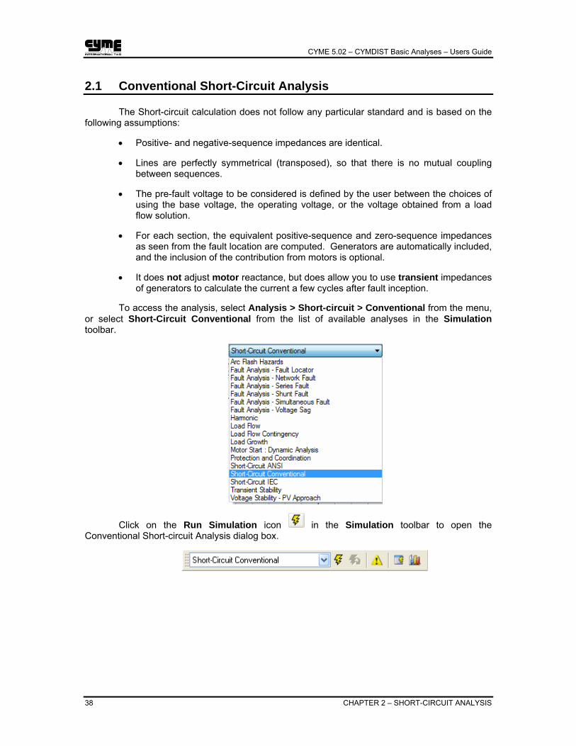
To access the analysis, select Analysis > Short-circuit > Conventional from the menu, or select Short-Circuit Conventional from the list of available analyses in the Simulation toolbar.
Click on the Run Simulation icon in the Simulation toolbar to open the Conventional Short-circuit Analysis dialog box.

CYME 5.02 – CYMDIST Basic Analyses – Users Guide
CHAPTER 2 – SHORT-CIRCUIT ANALYSIS 39
2.1.1 Fault Parameters Tab
This tab is used to make the fault selection and set appropriate general parameters for short-circuit calculations.
The program computes the fault current at every bus. A summary report is generated for all shunt fault types namely LLL, LG, LL and LL-G.
2.1.1.1 Fault Types
The fault types available to be analyzed are: LLL, LL, LLG, and LG. For each section, the software computes the equivalent positive-sequence and zero-sequence impedances as seen from the fault location. Generators are automatically included.
Three-phase Fault The current at the end of a line /cable or at a node/bus is calculated as follows:
ZfZVILLL +
=1
Where:
• V = pre-fault line-to-neutral voltage. Define this variable via the Pre-fault voltage block in the Fault Parameters tab.
• Z1 = cumulative positive-sequence impedance between the fault location and the substation, including the impedance of the substation.

CYME 5.02 – CYMDIST Basic Analyses – Users Guide
40 CHAPTER 2 – SHORT-CIRCUIT ANALYSIS
• Zf = impedance of the fault itself. Define this variable via Analysis > Short Circuit, Conventional Parameters tab.
• The safety (security) factors Kmax and Kmin can be applied to the calculated faults currents. Define this variable via Analysis > Short Circuit, Conventional Parameters tab.
Double-Line-to-Ground Fault The calculation of the LLG fault is done by computing the fault currents on phase
B and phase C using:
( ) ( )⎟⎟⎠
⎞⎜⎜⎝
⎛++++++
++=
ZgZfZZZgZfZZfZZfZ
VIa
322030*21
1
⎟⎟⎠
⎞⎜⎜⎝
⎛+++
+−=
ZgZfZZZfZII aa 3202
2*10
⎟⎟⎠
⎞⎜⎜⎝
⎛+++
++−=
ZgZfZZZgZfZII aa 3202
30*12
212
0_ aaabLLG aIIaII ++=
22
10_ aaacLLG IaaIII ++=
cLLGbLLGTLLG III ___ +=
Where:
• V = pre-fault line-to-neutral voltage. Define this variable via the Pre-fault voltage block in the Fault Parameters tab.
• Z0 = cumulative zero-sequence impedance between the fault location and the substation, including the impedance of the substation.
• Z2 = Z1 since it is assumed that the positive and negative sequence impedances are identical.
• Zf = impedance of the fault itself. Define this variable via Analysis > Short Circuit, Conventional Parameters tab.
• Zg = impedance to ground of the fault itself. Define this variable via Analysis > Short Circuit, Conventional Parameters tab.
• The safety (security) factors Kmax and Kmin can be applied to the calculated faults currents. Define this variable via Analysis > Short Circuit, Conventional Parameters tab.

CYME 5.02 – CYMDIST Basic Analyses – Users Guide
CHAPTER 2 – SHORT-CIRCUIT ANALYSIS 41
Line-to-Line Fault
ZfZVILL +
=12
*3
Where:
• V = pre-fault line-to-neutral voltage. Define this variable via the Pre-fault voltage block in the Fault Parameters tab.
• Z1 = cumulative positive-sequence impedance between the fault location and the substation, including the impedance of the substation.
• Zf = impedance of the fault itself. Define this variable via Analysis > Short Circuit, Conventional Parameters tab.
• The safety (security) factors Kmax and Kmin can be applied to the calculated faults currents. Define this variable via Analysis > Short Circuit, Conventional Parameters tab.
Single-Line-to-Ground Fault
ZgZZVILG 3012
*3++
=
Where:
• V = pre-fault line-to-neutral voltage. Define this variable via the Pre-fault voltage block in the Fault Parameters tab.
• Z1 = cumulative positive-sequence impedance between the fault location and the substation, including the impedance of the substation.
• Zg = impedance of the fault itself. Define this variable via Analysis > Short Circuit, Conventional Parameters tab.
• Z0 = cumulative zero-sequence impedance between the fault location and the substation, including the impedance of the substation.
• The safety (security) factors Kmax and Kmin can be applied to the calculated faults currents. Define this variable via Analysis > Short Circuit, Conventional Parameters tab.
Hint: The Double-Line-to-Ground fault current is the same as the Line-to-Line fault current on a Delta configuration line.
Asymmetry Factor
The (first half-cycle) asymmetry factor is calculated as: R/X2-2e+1=K ⋅π .
• R = cumulative positive-sequence resistance.
• X = cumulative positive-sequence reactance.
CYME 5.02 – CYMDIST Basic Analyses – Users Guide
42 CHAPTER 2 – SHORT-CIRCUIT ANALYSIS
Peak Factor
The (first half-cycle) peak factor is calculated as: ( )R/X-e12=K ⋅+⋅ π .
• R = cumulative positive-sequence resistance.
• X = cumulative positive-sequence reactance.
2.1.1.2 Calculation Parameters
The Fault Parameters tab contains more options one can select from to specify other factors to be considered in the short-circuit calculation.
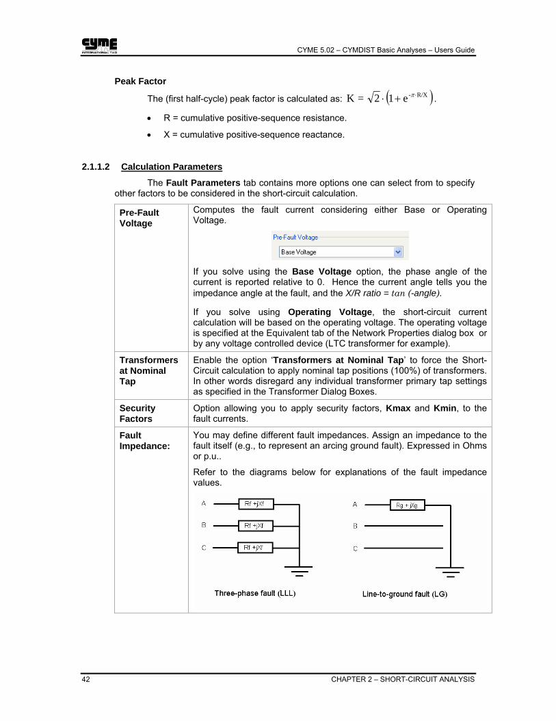
Pre-Fault Voltage
Computes the fault current considering either Base or Operating Voltage.
If you solve using the Base Voltage option, the phase angle of the current is reported relative to 0. Hence the current angle tells you the impedance angle at the fault, and the X/R ratio = tan (-angle).
If you solve using Operating Voltage, the short-circuit current calculation will be based on the operating voltage. The operating voltage is specified at the Equivalent tab of the Network Properties dialog box or by any voltage controlled device (LTC transformer for example).
Transformers at Nominal Tap
Enable the option ‘Transformers at Nominal Tap’ to force the Short-Circuit calculation to apply nominal tap positions (100%) of transformers. In other words disregard any individual transformer primary tap settings as specified in the Transformer Dialog Boxes.
Security Factors
Option allowing you to apply security factors, Kmax and Kmin, to the fault currents.
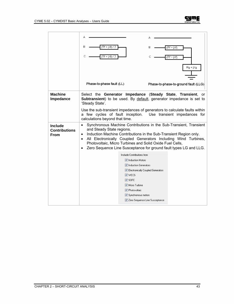
Fault Impedance:
You may define different fault impedances. Assign an impedance to the fault itself (e.g., to represent an arcing ground fault). Expressed in Ohms or p.u..
Refer to the diagrams below for explanations of the fault impedance values.
CYME 5.02 – CYMDIST Basic Analyses – Users Guide
CHAPTER 2 – SHORT-CIRCUIT ANALYSIS 43
Machine Impedance
Select the Generator Impedance (Steady State, Transient, or Subtransient) to be used. By default, generator impedance is set to ‘Steady State’.
Use the sub-transient impedances of generators to calculate faults within a few cycles of fault inception. Use transient impedances for calculations beyond that time.
Include Contributions From
• Synchronous Machine Contributions in the Sub-Transient, Transient and Steady State regions.
• Induction Machine Contributions in the Sub-Transient Region only. • All Electronically Coupled Generators Including Wind Turbines,
Photovoltaic, Micro Turbines and Solid Oxide Fuel Cells, • Zero Sequence Line Susceptance for ground fault types LG and LLG.

CYME 5.02 – CYMDIST Basic Analyses – Users Guide
44 CHAPTER 2 – SHORT-CIRCUIT ANALYSIS
2.1.2 Networks Tab
Select in the list the networks you wish to analyze. Click on the check box next to a network name to select or de-select it individually. Click on the symbol to expand the list and on to collapse it again. All selects every feeder loaded in the study. None de-selects all feeders.
CYME 5.02 – CYMDIST Basic Analyses – Users Guide
CHAPTER 2 – SHORT-CIRCUIT ANALYSIS 45
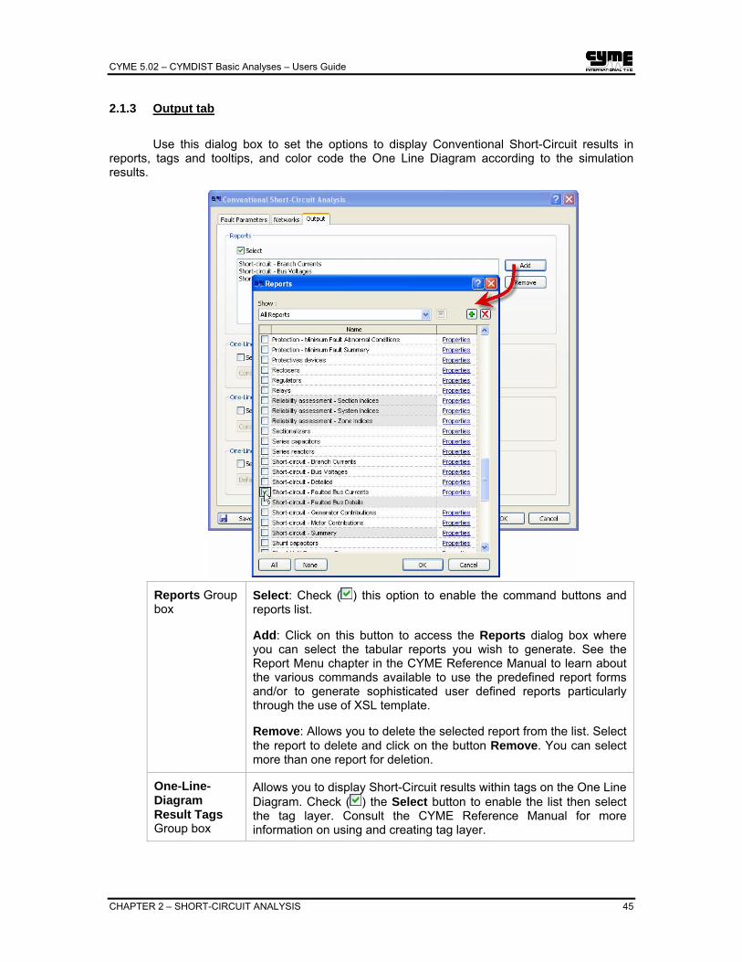
2.1.3 Output tab
Use this dialog box to set the options to display Conventional Short-Circuit results in reports, tags and tooltips, and color code the One Line Diagram according to the simulation results.
Reports Group box
Select: Check ( ) this option to enable the command buttons and reports list.
Add: Click on this button to access the Reports dialog box where you can select the tabular reports you wish to generate. See the Report Menu chapter in the CYME Reference Manual to learn about the various commands available to use the predefined report forms and/or to generate sophisticated user defined reports particularly through the use of XSL template.
Remove: Allows you to delete the selected report from the list. Select the report to delete and click on the button Remove. You can select more than one report for deletion.
One-Line-Diagram Result Tags Group box
Allows you to display Short-Circuit results within tags on the One Line Diagram. Check ( ) the Select button to enable the list then select the tag layer. Consult the CYME Reference Manual for more information on using and creating tag layer.

CYME 5.02 – CYMDIST Basic Analyses – Users Guide
46 CHAPTER 2 – SHORT-CIRCUIT ANALYSIS
One-Line-Diagram Color Coding Group box
Allows you to color-code the One Line Diagram based on the Short-Circuit results. Check ( ) the Select button to enable list then select the coloring layer. Consult to the CYME Reference Manual for more information on using and creating coloring layer.
One-Line-Diagram Tooltips Group box
Allows you to display Short-Circuit results within tooltips by hovering the mouse over a section on the One Line Diagram. Check ( ) the Select button to enable the list then select simulation whose results you want to see. Note that if you have activated the option Always run both simulation simultaneously in the tab Simulation of the Preferences dialog box, Load flow results will be available. Consult the CYME Reference Manual for more information on using and creating tooltips.
2.2 ANSI Short-Circuit Analysis
The ANSI Version follows the American National Standards Institute recommendations for circuit breaker application C37.010 (symmetrical current basis), C37.5 (total current basis) and C37.13 (low voltage circuit breakers):
• It calculates four specific duty types, according to the standards, and applies multipliers to the calculated currents to account for asymmetry in the short circuit current (DC component).
• It adjusts the reactance of motors according to their size and speed to account for the fact that their contribution to faults decays with time.
• It does not permit the inclusion of pre-fault load current. • It does not permit a fault impedance (Zf) since only “bolted” faults are allowed, as
stipulated in the standard. • It does not permit a grounding fault impedance (Zg). Only “bolted” faults are
permitted.
As stipulated in the ANSI standards, the ANSI short-circuit calculation performs the I = E/Z computation (using complex impedances in the network matrices) and computes X/R ratios by reducing separate X and R networks.
Three-phase fault: X / R = X1 / R1
Line-to-ground fault: X / R = (2 X1 + X0 ) / (2 R1 + R0)
Depending on the fault duty selected and the X/R ratio at the fault location, the ANSI short-circuit calculation identifies the multipliers to be applied to the symmetrical current to account for AC and DC decrements. Different multipliers apply to current contributions from local and remote sources. Note that if the X/R is less than 15, no multipliers are needed.
Select Short-circuit ANSI from the list of available analyses in the Simulation toolbar. You may also select Analysis > Short-circuit > ANSI from the menu.

CYME 5.02 – CYMDIST Basic Analyses – Users Guide
CHAPTER 2 – SHORT-CIRCUIT ANALYSIS 47
Click on the Run Simulation icon in the Simulation toolbar to open the ANSI Short-circuit Analysis dialog box.
2.2.1 ANSI Parameters Tab
This tab is used to set the ANSI short-circuit duty type calculations.
The program computes the fault current at every bus. A summary report is generated for all shunt fault types namely LLL, LG, LL and LL-G.

CYME 5.02 – CYMDIST Basic Analyses – Users Guide
48 CHAPTER 2 – SHORT-CIRCUIT ANALYSIS
2.2.1.1 DUTY Type
There are four available DUTY types as defined in the standards: Closing /Latching
The symmetrical RMS current is calculated at one-half cycle after fault inception. According to the standard ANSI C37.010, the symmetrical current is multiplied by 1.6 to account for asymmetry due to the DC component. The resulting current is the so-called “momentary” rating used to evaluate the circuit breaker’s capability to close into a faulted circuit and remain closed (“latched”) until tripped. The peak current (symmetrical RMS x 2.6) are also reported to facilitate comparison of the current against preferred breaker ratings (standard C37.06).
More realistic multipliers are also computeed, using the actual X/R ratio. It reports both the multiplier and the current adjusted by that multiplier.
( ) ( )I I IRMS asym AC RMS sym DC, , ,= +2 2 ( )= + −IAC RMS sym t X Re, , /1 2 4π
( )( )I IPEAK AC RMS sym t X Re= ⋅ −+, , /2 1 2π
Where t = 1/2 cycle.
To account for the decay of the motor contributions within the first half-cycle, the standards multiply the reactance of each motor by a factor determined from the motor power and speed:
Motor type Positive sequence reactance
for momentary duty All synchronous motors 1.0 X”d Induction motors
above 1000 HP at 1800 rpm or less 1.0 X”d above 250 HP at 3600 rpm 1.0 X”d all others 50 HP and above 1.2 X”d all smaller than 50 HP 1.67 X”d
Low Voltage CB
The symmetrical RMS current is calculated at one-half cycle after fault inception. If the fault X/R ratio exceeds the X/R on which the breaker rating is based, then according to ANSI standard C37.13, the symmetrical current is multiplied by a factor which depends on the fault X/R ratio.
[ ]MF
e X R
=+ −2 1
2 29
π /( / )
. for infused circuit breakers (if X/R > 6.6)
MF e X R=
+ −1 2125
2π /( / )
. for fused circuit breakers (if X/R > 4.9)
Motor reactance(s) are adjusted as Closing/Latching. Note: Results for Low Voltage circuit Breaker duty will be reported only
at buses whose base voltage is less than 1.0 kV.
CYME 5.02 – CYMDIST Basic Analyses – Users Guide
CHAPTER 2 – SHORT-CIRCUIT ANALYSIS 49
Contact Parting
The symmetrical RMS current is calculated at a point in time (within a few cycles after fault inception) when medium- and high-voltage circuit breakers try to interrupt it. Standard C37.010 provides graphs of multipliers to be applied to the symmetrical current which account for decay with time of the DC component and the AC current magnitude. These multipliers depend on the X/R ratio and the delay before the breaker begins to interrupt the current. (Standard C37.5 presents similar figures.)
See standard C37.010 for figures 8, 9 and 10 which each consist of four graphs (for 2-cycle, 3-cycle, 5-cycle and 8-cycle breaker speeds). Each graph shows the multiplier as a function of the X/R ratio for several values of contact parting time. The contact parting time is the sum of the tripping delay and about one half the time taken by the breaker to interrupt the current (breaker “speed”).
Figure 8 of the Standard gives the multiplier for three-phase fault current which is affected by both DC and AC decay (i.e., contributions from local sources). Figure 9 does the same for line-to-ground fault current. Figure 10 applies to current contributions to both fault types from remote (electrically distant) sources and assumes no AC decay. A contribution from a generator is classified as local if the impedance between the generator and the fault is less than 1.5 times the generator’s own sub-transient impedance. (See ANSI/IEEE C37.010). Otherwise the contribution is remote. Note that contributions from swing generators are always considered remote, because the swing is assumed to represent electrically distant generation.
Despite the fact that motor-contributions AC-decay is accounted according to the following table, you have the possibility to take into account motor contribution either as “local” or “remote”.
The application identifies the portions of the fault current which come from local and remote sources. For each contribution it finds the multiplier from its digitized version of the curves. It then finds the weighted sum:
I = (local multiplier)·(local current) + (remote multiplier)·(remote current)
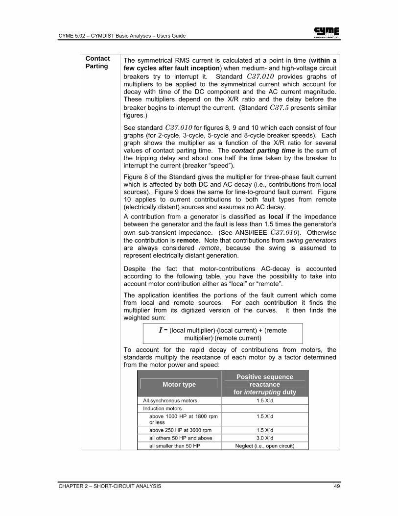
To account for the rapid decay of contributions from motors, the standards multiply the reactance of each motor by a factor determined from the motor power and speed:
Motor type Positive sequence
reactance for interrupting duty
All synchronous motors 1.5 X”d Induction motors
above 1000 HP at 1800 rpm or less
1.5 X”d
above 250 HP at 3600 rpm 1.5 X”d all others 50 HP and above 3.0 X”d all smaller than 50 HP Neglect (i.e., open circuit)

CYME 5.02 – CYMDIST Basic Analyses – Users Guide
50 CHAPTER 2 – SHORT-CIRCUIT ANALYSIS
Time Delayed The symmetrical RMS current is calculated at a point in time (say 30 cycles
after fault inception) when the contributions from motors have decayed to zero and the generators are represented by their transient reactance. There is no asymmetry in the current waveform and no multipliers are needed. No motor contribution is included for this duty type.
2.2.1.2 Include Contributions From
It is possible to select to include the contributions from induction machines, synchronous motors, other generation sources such as WECS and SOFC, and/or sequence line susceptance.
2.2.2 Networks Tab
Select in the list the networks you wish to analyze. Click on the check box next to a network name to select or de-select it individually. Click on the symbol to expand the list and on to collapse it again. All selects every feeder loaded in the study. None de-selects all feeders.

CYME 5.02 – CYMDIST Basic Analyses – Users Guide
CHAPTER 2 – SHORT-CIRCUIT ANALYSIS 51
2.2.3 Output Tab
Use this dialog box to set the options to display ANSI Short-Circuit results in reports, tags and tooltips, and color code the One Line Diagram according to the simulation results.
Reports Group box
Select: Check ( ) this option to enable the command buttons and reports list.
Add: Click on this button to access the Reports dialog box where you can select the tabular reports you wish to generate. See the Report Menu chapter in the CYME Reference Manual to learn about the various commands available to use the predefined report forms and/or to generate sophisticated user defined reports particularly through the use of XSL template.
Remove: Allows you to delete the selected report from the list. Select the report to delete and click on the button Remove. You can select more than one report for deletion.
One-Line-Diagram Result Tags Group box
Allows you to display Short-Circuit results within tags on the One Line Diagram. Check ( ) the Select button to enable the list then select the tag layer. Consult the CYME Reference Manual for more information on using and creating tag layer.

CYME 5.02 – CYMDIST Basic Analyses – Users Guide
52 CHAPTER 2 – SHORT-CIRCUIT ANALYSIS
One-Line-Diagram Color Coding Group box
Allows you to color-code the One Line Diagram based on the Short-Circuit results. Check ( ) the Select button to enable list then select the coloring layer. Consult to the CYME Reference Manual for more information on using and creating coloring layer.
One-Line-Diagram Tooltips Group box
Allows you to display Short-Circuit results within tooltips by hovering the mouse over a section on the One Line Diagram. Check ( ) the Select button to enable the list then select simulation whose results you want to see. Note that if you have activated the option Always run both simulation simultaneously in the tab Simulation of the Preferences dialog box, Load flow results will be available. Consult the CYME Reference Manual for more information on using and creating tooltips.
2.3 IEC Short-Circuit Analysis
The IEC analysis follows the European IEC 60909 guidelines for short circuit analysis applicable to three-phase AC systems at both 50 Hz and 60 Hz. It allows calculating:
• The initial, peak and breaking fault currents in networks of any configuration (radial or meshed).
• The steady state fault currents taking into account the saturated direct axis reactance and excitation characteristics of the contributing synchronous machines.
• The initial, peak and breaking current motor contributions according to the procedures tabulated in IEC for faults at motor terminals. The necessary multipliers are also calculated and reported depending on the type of duty under consideration. Both ac and dc offset currents are computed and reported.
• The maximum and minimum fault currents as stipulated in IEC 60909.
However, it does not allow: • The inclusion of pre-fault load current. At the fault point, the pre-fault voltage is
taken to be Cf times the system rated voltage. The factor Cf is defined in compliance with IEC 909 and may pertain to either maximum or minimum fault current calculations.
• The use of load flow solution voltages. • A fault impedance since only “bolted” faults are allowed, as stipulated in the
standard. • Switching from sub-transient to transient impedances because only sub-transient
generator impedances can be considered for all types of duty.
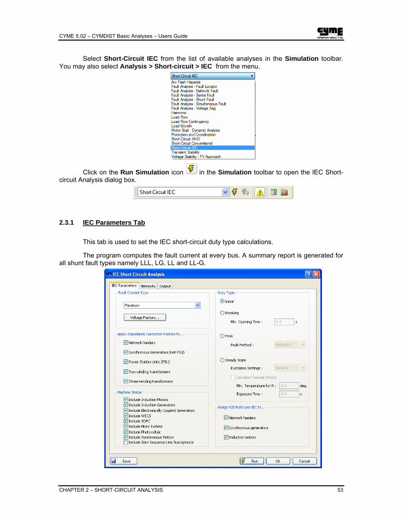
CYME 5.02 – CYMDIST Basic Analyses – Users Guide
CHAPTER 2 – SHORT-CIRCUIT ANALYSIS 53
Select Short-Circuit IEC from the list of available analyses in the Simulation toolbar. You may also select Analysis > Short-circuit > IEC from the menu.
Click on the Run Simulation icon in the Simulation toolbar to open the IEC Short-circuit Analysis dialog box.
2.3.1 IEC Parameters Tab
This tab is used to set the IEC short-circuit duty type calculations.
The program computes the fault current at every bus. A summary report is generated for all shunt fault types namely LLL, LG, LL and LL-G.

CYME 5.02 – CYMDIST Basic Analyses – Users Guide
54 CHAPTER 2 – SHORT-CIRCUIT ANALYSIS
2.3.1.1 Fault Current Type
The method used for calculation is based on the introduction of an equivalent voltage source at the short-circuit location. The equivalent voltage source is the only active voltage of the system. All network feeders, synchronous and asynchronous machines are replaced by their internal impedances.
In all cases, it is possible to determine the short-circuit current at the short-circuit location with the help of an equivalent voltage source. Operational data and the load of consumers, tap changer position of transformers, excitation of generators, and so on, are dispensable; additional calculations about all the different possible load flows of short circuit are superfluous.
In general, two short-circuit currents, which differ in their magnitude, are to be calculated:
• The maximum short-circuit current which determines the capacity or rating of electrical equipment: its calculation assumes that the pre-fault voltage of the aforesaid equivalent voltage source is Cf = Cmax times the system rated voltage at the fault location.
• The minimum short-circuit current which can be a basis, for example, for the selection of fuses, for the setting of protective devices, and for checking the run-up of motors: its calculation assumes that the pre-fault voltage of the aforesaid equivalent voltage source is Cf = Cmin times the system rated voltage at the fault location.
These voltage factors Cf can be set by clicking on the Voltage Factors button of the IEC tab; this will open the following dialog box:
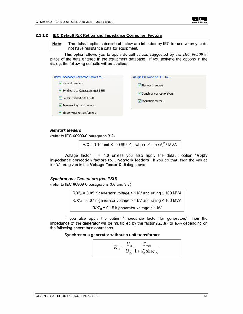
CYME 5.02 – CYMDIST Basic Analyses – Users Guide
CHAPTER 2 – SHORT-CIRCUIT ANALYSIS 55
2.3.1.2 IEC Default R/X Ratios and Impedance Correction Factors
Note: The default options described below are intended by IEC for use when you do not have resistance data for equipment.
This option allows you to apply default values suggested by the IEC 60909 in place of the data entered in the equipment database. If you activate the options in the dialog, the following defaults will be applied:
Network feeders (refer to IEC 60909-0 paragraph 3.2)
R/X = 0.10 and X = 0.995 Z, where Z = c(kV)2 / MVA
Voltage factor c = 1.0 unless you also apply the default option “Apply impedance correction factors to… Network feeders”. If you do that, then the values for “c” are given in the Voltage Factor C dialog above.
Synchronous Generators (not PSU) (refer to IEC 60909-0 paragraphs 3.6 and 3.7)
R/X”d = 0.05 if generator voltage > 1 kV and rating ≥ 100 MVA
R/X”d = 0.07 if generator voltage > 1 kV and rating < 100 MVA
R/X”d = 0.15 if generator voltage ≤ 1 kV
If you also apply the option “impedance factor for generators”, then the impedance of the generator will be multiplied by the factor KG, KS or KSO depending on the following generator’s operations.
Synchronous generator without a unit transformer
rGdrG
nG x
CUU
Kϕsin1
max
′′+=
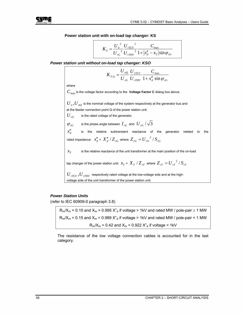
CYME 5.02 – CYMDIST Basic Analyses – Users Guide
56 CHAPTER 2 – SHORT-CIRCUIT ANALYSIS
Power station unit with on-load tap changer: KS
rGTdrTHV
rTLV
rG
nS xx
CUU
UUK
ϕsin1max
2
2
2
2
−′′+=
Power station unit without on-load tap changer: KSO
rGdrTHV
rTLV
rG
nQOS x
CUU
UU
Kϕsin1
max
′′+=
where
maxC is the voltage factor according to the Voltage Factor C dialog box above.
nQn UU , is the nominal voltage of the system respectively at the generator bus and
at the feeder connection point Q of the power station unit.
rGU is the rated voltage of the generator.
rGϕ is the phase angle between rGI and 3/rGU
dx ′′ is the relative subtransient reactance of the generator related to the
rated impedance: dx ′′ = rGd ZX /′′ where rGrGrG SUZ /2=
Tx is the relative reactance of the unit transformer at the main position of the on-load
tap changer of the power station unit: Tx = rTT ZX / where rTrTrT SUZ /2=
rTHVrTLV UU , respectively rated voltage at the low-voltage side and at the high-
voltage side of the unit transformer of the power station unit.
Power Station Units (refer to IEC 60909-0 paragraph 3.8)
Rm/Xm = 0.10 and Xm = 0.995 X”d if voltage > 1kV and rated MW / pole-pair ≥ 1 MW
Rm/Xm = 0.15 and Xm = 0.989 X”d if voltage > 1kV and rated MW / pole-pair < 1 MW
Rm/Xm = 0.42 and Xm = 0.922 X”d if voltage < 1kV The resistance of the low voltage connection cables is accounted for in the last category.

CYME 5.02 – CYMDIST Basic Analyses – Users Guide
CHAPTER 2 – SHORT-CIRCUIT ANALYSIS 57
Two- and three-winding transformers (refer to IEC 60909-0 paragraph 3.3.3)
For two-winding transformers with and without on-load tap changer, an impedance correction factor KT is to be multiplied with the transformer impedance.
TT x
CK
6.0195.0 max
+=
maxC is the voltage factor related to the nominal voltage of the low-voltage side bus of the transformer
according to the Voltage Factor C table above.
Tx is the relative reactance of the transformer:
Tx = rTT ZX / where rTrTrT SUZ /2=
For three-winding transformers, three impedance correction factors can be found using the relative values of the reactance of the transformers.
TPSTPS x
CK
6.0195.0 max
+=
TPTTPT x
CK
6.0195.0 max
+=
TSTTST x
CK
6.0195.0 max
+=
TPSx , TPTx and TSTx are respectively the imaginary parts of the relative transformer impedances
measured between primary-secondary, primary-tertiary and secondary-tertiary asked in the transformer database dialog.
2.3.1.3 Machine Status
To take into account motor, co-generation fault contributions and zero sequence line susceptance activate these options.

CYME 5.02 – CYMDIST Basic Analyses – Users Guide
58 CHAPTER 2 – SHORT-CIRCUIT ANALYSIS
2.3.1.4 Duty Types
According to IEC, four types of fault currents are of interest to industrial fault studies. Initial Short-circuit Current (I"k)
The (50 Hz or 60 Hz) RMS fault current flowing immediately after the occurrence of the short-circuit.
Peak Asymmetrical Fault Current (Ip)
The highest instantaneous value of the fault current after the fault occurrence. The software calculates the worst case peak current according to the standard.
Breaking Fault Current (Ib)
The RMS value of the symmetrical fault current flowing through the first phase to open when contact separation occurs in the circuit breaker. This quantity depends on the breaker opening time.
Steady State Fault Current (Ik)
The RMS value of the symmetrical fault current which remains after all transients have died away. This quantity depends, among other things, on the excitation characteristics of the generators feeding the fault. The software supports all excitation system modes stipulated in the IEC 60909 standard.
2.3.2 Networks Tab
Select in the list the networks you wish to analyze. Click on the check box next to a network name to select or de-select it individually. Click on the symbol to expand the list and on to collapse it again. All selects every feeder loaded in the study. None de-selects all feeders.

CYME 5.02 – CYMDIST Basic Analyses – Users Guide
CHAPTER 2 – SHORT-CIRCUIT ANALYSIS 59
2.3.3 Output Tab
Use this dialog box to set the options to display the results in reports, tags and tooltips and color code the One Line Diagram according to the simulation results.
Reports Group box
Select: Check ( ) this option to enable the command buttons and reports list.
Add: Click on this button to access the Reports dialog box. where you can select the tabular reports you wish to generate. See the Report Menu chapter in the CYME Reference Manual to learn about the various commands available to use the predefined report forms and/or to generate sophisticated user defined reports particularly through the use of XSL template.
Remove: Allows you to delete the selected report from the list. Select the report to delete and click on the button remove. You can select more than one report for deletion.
One-Line-Diagram Result Tags Group box
Allows you to display the results within tags on the One Line Diagram. Check ( ) the Select button to enable the list then select the tag layer. Consult the CYME Reference Manual for more information on using and creating tag layer.

CYME 5.02 – CYMDIST Basic Analyses – Users Guide
60 CHAPTER 2 – SHORT-CIRCUIT ANALYSIS
One-Line-Diagram Color Coding Group box
Allows you to color-code the One Line Diagram based on the simulation results. Check ( ) the Select button to enable list then select the coloring layer. Consult to the CYME Reference Manual for more information on using and creating coloring layer.
One-Line-Diagram Tooltips Group box
Allows you to display simulation results within tooltips by hovering the mouse over a section on the One Line Diagram. Check ( ) the Select button to enable the list then select simulation whose results you want to see. Note that if you have activated the option Always run both simulation simultaneously in the tab Simulation of the Preferences dialog box, Short-circuit results will be available. Consult the CYME Reference Manual for more information on using and creating tooltips.
2.4 Results
2.4.1 Reports
You may select the items to be reported via the command Report > On Calculation…, or through the Output tab prior to running the analysis.
Click on the Properties hyperlink to customize the report with any of the keywords available.

CYME 5.02 – CYMDIST Basic Analyses – Users Guide
CHAPTER 2 – SHORT-CIRCUIT ANALYSIS 61
Click on the button twice to generate the report. Here is a sample of a short-circuit detailed report.
Sample Short-circuit detailed report, available for the Short-Circuit on all buses and nodes calculation option
See the Report Menu chapter in the CYME Reference Manual to learn about the various commands available to profit from predefined reports and/or to generate sophisticated user defined reports particularly through the use of XSL template.
2.4.2 Report by Individual Section
To see the report by individual section, first display the Short-Circuit Box via View > Result Box > Short-Circuit Box, and then click on a section on the one-line display.
Hint: You can use the keyboard shortcut <Ctrl> + <S> to hide or show the Short-Circuit Box (Ref: Customize > Shortcuts).
The description of the default data reported in the Short-Circuit Results Box are detailed below. (Note: the contents of the Short Circuit Results Box can be customized.)
LLL three-phase fault current, in Amperes.
LLG double-line-to-ground fault current, in Amperes.
LL line-to-line fault current, in Amperes.
LG line-to-ground fault current, in Amperes.

CYME 5.02 – CYMDIST Basic Analyses – Users Guide
62 CHAPTER 2 – SHORT-CIRCUIT ANALYSIS
Choice of measurement location. See diagram below, and recall from Section Structure that there may be 3 sub-sections in a section.
One or two of the circles will not be active if no equipment is connected, which would divide the section into sub-sections.
The three locations for measuring fault currents.
Sample customizable result box to show the results of a Single Fault Calculation – resulting voltages and currents in phase and in sequence.
The last four buttons of the Result box ( ) will help monitor multiple locations. See the Customize Menu chapter of the CYME Reference Manual, under Result Boxes.

CYME 5.02 – CYMDIST Basic Analyses – Users Guide
CHAPTER 2 – SHORT-CIRCUIT ANALYSIS 63
2.4.3 Charts
Click on the button inside the Short Circuit Box (Results) to display the Chart Selection dialog box where you can select to plot the fault current profile along the feeder, from the substation to the active section. See below.
Note on the profile: The customization of the Profiles may be done through the menu Customize > Charts (or by clicking on the Customize button in the Chart Selection dialog box). See the CYME Reference Manual for further information.
Note that the Short Circuit Box is superimposed on the plot. You may hide it temporarily by closing its window. (Press <Ctrl> + <S> to get it back again.)
Hint: If you make any changes to the feeder, such as adding a load, the program will discard all of the analysis results, and the results box will disappear.

CYME 5.02 – CYMDIST Basic Analyses – Users Guide
64 CHAPTER 2 – SHORT-CIRCUIT ANALYSIS
2.4.4 Report Tags
Short-circuit results may be displayed on the One Line Diagram, next to the sections, inside Report Tags and/or in the Tool Tip. See the example below.
2.4.5 One-Line Diagram Coloring
The one-line diagram can be color-coded based on the short-circuit results. You can select from a list of predefined coloring layers or you can create your own color coding layer. You may select the active color coding layer using the Color Coding Layer toolbar. You can create and completely customize your own color coding; to do so, use the Customize > Color coding menu command. Consult to the CYME Reference Manual for more information.
Hint: Use the color-coding by fault level to predict fault location using the short circuit current magnitude.
Suppose that you would like to determine the possible locations of a Fault with a magnitude of 600A.
You could enable thresholds with colors:
• BLUE for 1 to 595A
• RED for 596 to 605A
• GREEN for 606 to 10000A.
Then the possible sections will be displayed in RED.

CYME 5.02 – CYMDIST Basic Analyses – Users Guide
CHAPTER 3 – FAULT ANALYSIS 65
Chapter 3 Fault Analysis
Electrical distribution networks are susceptible to faults due to various causes such as weather conditions, equipment failures, animals, etc. These faults result in power interruptions that affect the customer’s power quality.
Since reliability is a major concern, it is very important to locate and identify faults effectively, to know the highest possible short circuit level at a given location on the network.
Tools available are:
• Shunt Fault Analysis – to compute all possible fault currents at a selected location. • Network Fault Analysis – to compute all possible fault currents at multiple locations
and to evaluate generator contributions • Voltage Sag – to study the impact of a sudden reduction of voltage magnitude
caused by network faults, or other disturbances such as motor starting or overloads. • Fault Locator – to evaluate possible locations of a fault on the network
3.1 Shunt Fault Analysis
The Fault Analysis: Shunt Fault Option Computes the fault current at a selected bus/node/line/cable and reports the voltages and currents on the entire network including any machine contributions.
System wide voltages, branch currents and machine contributions are all reported on the network one line diagram and in the selected reports.
Calculation Assumptions: • The Pre-fault Voltage is taken into account during the calculation. • Motors will be considered as current injecting sources in series with the internal sub-
transient impedance of the specific motor • Generators, during the fault, will be represented by their sub-transient impedance. • Power lines coming from the outside of the single line diagram will be considered as
infinite sources limited only by their impedance connected in series (Specifically, Positive and zero sequence impedances are considered)
• Protective devices (fuses, reclosers, etc.) cannot react quickly enough so that they will be considered frozen. This is also true for any automated equipment (LTC, AGC, etc.)
Calculation Limitations: • Loads and shunt capacitors loads will be considered as constant impedance loads. • The neutral wire is to be considered at zero voltage. • If the network configuration is not providing a stable solution (i.e. convergent
solution), the fault flow calculation will not converge either. • The command will block cases that could not be attempted in real life (for example,
attempting to apply a LL fault to WYE-Delta transformer 2 wires to 1 wire). • Only one fault can be presented at any given time. • The section selected must be connected to a source (i.e. substation or an equivalent)

CYME 5.02 – CYMDIST Basic Analyses – Users Guide
66 CHAPTER 3 – FAULT ANALYSIS
Select Analysis > Fault Analysis > Shunt Fault to calculates the load flow of a network system (looped or radial) when a fault is applied to a specific section.
3.1.1 Parameters Tab
Shunt Fault Method Group box
Select the Short-circuit Method as either Conventional, ANSI or IEC.
The user can also access and modify the short-circuit parameters
with the tab.
In addition, the phase or sequence domain can be specified for the analysis.

CYME 5.02 – CYMDIST Basic Analyses – Users Guide
CHAPTER 3 – FAULT ANALYSIS 67
Shunt Fault Location Group box
Computes the fault current at a selected bus/node/line/cable and reports the voltages and currents on the entire network including any machine contributions.
If a single fault at a line or a cable is selected then At field will become active to allow specifying the location of the fault along the line or cable.
This will eliminate the need to subdivide the line or cable with intermediate nodes or buses to simulate this type of fault.
Fault Type Group Box
You can select the fault type as LLL, LL, LL-G, L-G or ALL faults. Selecting this option will compute all shunt fault at the desired location.
In addition, if the Phase Domain is selected, then the user can select which of the phase(s) are to be faulted. A LG fault example is shown for reference.

CYME 5.02 – CYMDIST Basic Analyses – Users Guide
68 CHAPTER 3 – FAULT ANALYSIS
3.1.2 Output Tab
Use this dialog box to set the options to display the results in reports, tags and tooltips and color code the One Line Diagram according to the simulation results.
Reports Group box
Select: Check ( ) this option to enable the command buttons and reports list.
Add: Click on this button to access the Reports dialog box. where you can select the tabular reports you wish to generate. See the Report Menu chapter in the CYME Reference Manual to learn about the various commands available to use the predefined report forms and/or to generate sophisticated user defined reports particularly through the use of XSL template.
Remove: Allows you to delete the selected report from the list. Select the report to delete and click on the button remove. You can select more than one report for deletion.
One-Line-Diagram Result Tags Group box
Allows you to display the simulation results within tags on the One Line Diagram. Check ( ) the Select button to enable the list then select the tag layer. Consult the CYME Reference Manual for more information on using and creating tag layer.

CYME 5.02 – CYMDIST Basic Analyses – Users Guide
CHAPTER 3 – FAULT ANALYSIS 69
One-Line-Diagram Color Coding Group box
Allows you to color-code the One Line Diagram based on the simulation results. Check ( ) the Select button to enable list then select the coloring layer. Consult to the CYME Reference Manual for more information on using and creating coloring layer.
One-Line-Diagram Tooltips Group box
Allows you to display the simulation results within tooltips by hovering the mouse over a section on the One Line Diagram. Check ( ) the Select button to enable the list then select simulation whose results you want to see. Note that if you have activated the option Always run both simulation simultaneously in the tab Simulation of the Preferences dialog box, Short-circuit results will be available. Consult the CYME Reference Manual for more information on using and creating tooltips.
3.1.3 Shunt Fault Results
Reports, if selected from the Output tab of the Shunt Fault Analysis dialog box, should be displayed automatically upon completion of the analysis. Or, the user can choose to display reports by accessing Reports > On Calculation.
Sample Shunt Fault-Branch current report
To see the report by individual section, first display the Load Flow Box via View > Result Box > Load Flow Box, and then click on a section on the one-line display.
Hint: You can use the keyboard shortcut <Ctrl> + <V> to hide or show the Load Flow Box (Ref: Customize > Shortcuts).

CYME 5.02 – CYMDIST Basic Analyses – Users Guide
70 CHAPTER 3 – FAULT ANALYSIS
3.2 Network Fault Analysis The Network Fault Module is a feature that will automatically calculate the highest and
lowest short circuit currents at the desired nodes.
With this new powerful tool, it is possible to: • Calculate the highest and lowest currents at a given network location • Calculate the highest and lowest voltages at the points of interest • Rate protective equipment and settings based on maximum currents • Determine highest/lowest generator contributions The Network Fault module will significantly help power engineers to make fast decisions
by providing them with accurate detailed information about the maximum and minimum faults occurring at the points of interest and allow protecting the network accordingly.
To run the analysis, access Analysis > Fault Analysis > Network Fault. You may also select it from the Simulation toolbar.
3.2.1 Parameters Tab

CYME 5.02 – CYMDIST Basic Analyses – Users Guide
CHAPTER 3 – FAULT ANALYSIS 71
Shunt Fault Location
The fault location is where the shunt fault will be applied. Shunt faults can only be applied to buses or nodes. It is possible to select as many buses/nodes as desired.
Monitoring items
The monitoring items are equipment where the results are to be displayed. If buses or nodes are selected, voltage reports will be displayed. If branches are selected (transformers, cables, etc), current reports will be displayed.
Shunt Fault Method
There are 3 short-circuit methods available: Conventional short circuit, ANSI short circuit and IEC short circuit. The Parameters button can be used to configure the short circuit parameters to be used for the simulation. It is important to note that the parameters as set here are only applicable to the Network Fault analysis and are not global parameters applicable to Shunt Fault analysis.
The calculation can be performed in the Phase domain or in the Sequence domain.
Fault Type There are four types of fault that can be calculated: 3 phase LLL fault, single phase LG fault, LL and LLG faults.
Reports There are two types of reports available: a min/max report that displays only the maximum and minimum results for every monitored bus/node or a Detailed summary report that displays currents at the monitored buses/nodes for all faulted bus/nodes.
Units The tabular results can be either displayed in amps/volts or in per-unit.. Results The results displayed in the report can be in Phase domain or in
Sequence domain.
3.2.2 Results
The results of this analysis are given in a tabular format. Only the selected reports will be generated. The summary report gives detailed information about the monitored nodes.
The min/max report gives only the minimum and maximum current values at every monitored node and displays what node produced that current.

CYME 5.02 – CYMDIST Basic Analyses – Users Guide
72 CHAPTER 3 – FAULT ANALYSIS
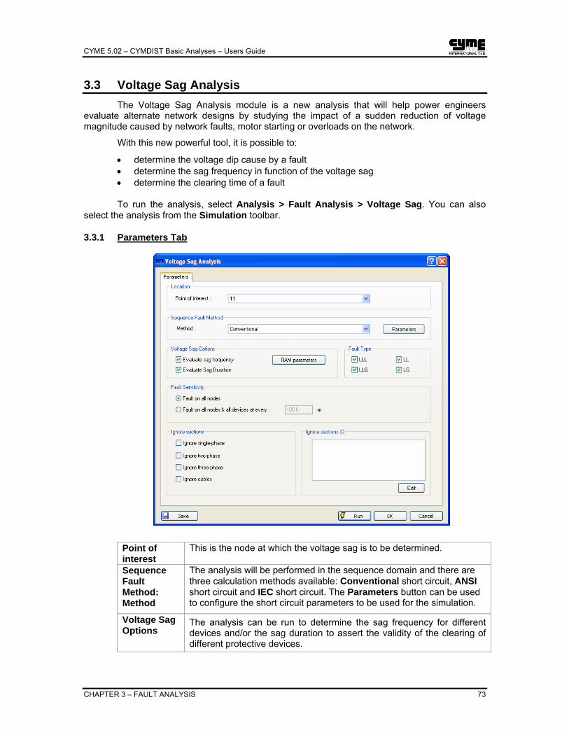
CYME 5.02 – CYMDIST Basic Analyses – Users Guide
CHAPTER 3 – FAULT ANALYSIS 73
3.3 Voltage Sag Analysis The Voltage Sag Analysis module is a new analysis that will help power engineers
evaluate alternate network designs by studying the impact of a sudden reduction of voltage magnitude caused by network faults, motor starting or overloads on the network.
With this new powerful tool, it is possible to:
• determine the voltage dip cause by a fault • determine the sag frequency in function of the voltage sag • determine the clearing time of a fault To run the analysis, select Analysis > Fault Analysis > Voltage Sag. You can also
select the analysis from the Simulation toolbar.
3.3.1 Parameters Tab
Point of interest
This is the node at which the voltage sag is to be determined.
Sequence Fault Method: Method
The analysis will be performed in the sequence domain and there are three calculation methods available: Conventional short circuit, ANSI short circuit and IEC short circuit. The Parameters button can be used to configure the short circuit parameters to be used for the simulation.
Voltage Sag Options
The analysis can be run to determine the sag frequency for different devices and/or the sag duration to assert the validity of the clearing of different protective devices.
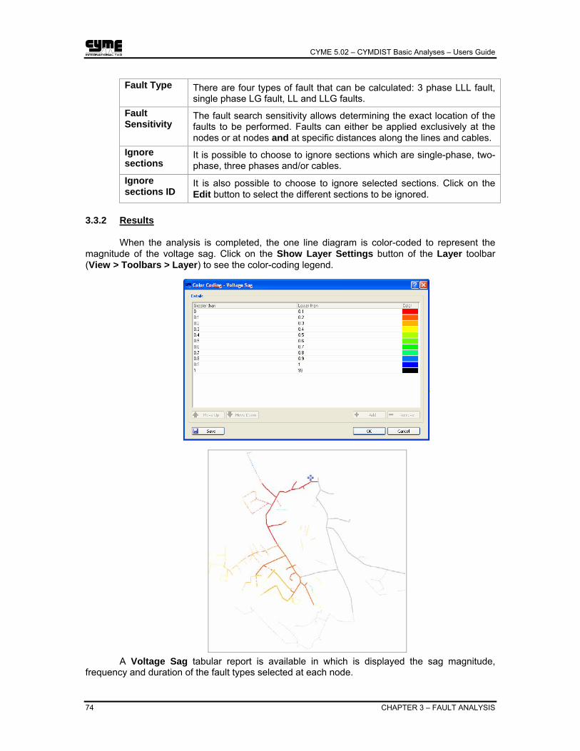
CYME 5.02 – CYMDIST Basic Analyses – Users Guide
74 CHAPTER 3 – FAULT ANALYSIS
Fault Type There are four types of fault that can be calculated: 3 phase LLL fault, single phase LG fault, LL and LLG faults.
Fault Sensitivity
The fault search sensitivity allows determining the exact location of the faults to be performed. Faults can either be applied exclusively at the nodes or at nodes and at specific distances along the lines and cables.
Ignore sections
It is possible to choose to ignore sections which are single-phase, two-phase, three phases and/or cables.
Ignore sections ID
It is also possible to choose to ignore selected sections. Click on the Edit button to select the different sections to be ignored.
3.3.2 Results
When the analysis is completed, the one line diagram is color-coded to represent the magnitude of the voltage sag. Click on the Show Layer Settings button of the Layer toolbar (View > Toolbars > Layer) to see the color-coding legend.
A Voltage Sag tabular report is available in which is displayed the sag magnitude,
frequency and duration of the fault types selected at each node.

CYME 5.02 – CYMDIST Basic Analyses – Users Guide
CHAPTER 3 – FAULT ANALYSIS 75
Charts are also plotted to show a more graphical representation of the results. Sag
Frequency VS Magnitude, Cumulative Sag Frequency VS Sag Magnitude, as well as Voltage Sag in function of clearing are plotted.
3.4 Fault Locator Analysis The Fault Locator module is a new analysis that will help power engineers locating the
faults on electrical network.
With this new powerful tool, it is possible to: • determine the type of the occurring fault (LG, LL or LLL) • determine the distance from the point of measure • rank the possible locations in the network The Fault Locator analysis is a post-mortem type of analysis. Based on a given short
circuit level recorded at a known location, the objective is to find all possible locations in the network where a short circuit could have occurred producing the recorded magnitude.
The fault location module will significantly help power engineers to make fast decisions
by providing them with accurate detailed information about the fault occurring in the network. Here are some advantages that this module offers:
• less inspection time to identify problems • faster dispatch of operators to repair the fault, transfer loads, etc • in cases where multiple locations are possible, the ranking of the location will make
the inspection more efficient

CYME 5.02 – CYMDIST Basic Analyses – Users Guide
76 CHAPTER 3 – FAULT ANALYSIS
To run the analysis, select Analysis > Fault Analysis > Fault Locator. You can also select the analysis from the Simulation toolbar.
3.4.1 Parameters Tab
Location This is the section at which the fault current is recorded. The location
can be either a protective device such a fuse, switch, recloser, sectionalizer or a branch such as a line or cable
Fault Recorded This field specifies the magnitude of the fault current that was recorded, in phase domain or in the sequence domain.
Fault Type The type of the fault current recorded can be specified. Fault types available are LLL, LLG, LL and LG. The analysis will only find locations with the fault current of matching fault type(s). If the fault type is unknown, select all four types.
Method There are 3 short-circuit methods available: Conventional short circuit, ANSI short circuit and IEC short circuit. The Parameters button can be used to configure the short circuit parameters to be used for the simulation.
Fault search sensitivity The Fault search sensitivity allows determining the locations at
which the fault is to be simulated. Faults can either be applied at all the nodes or at nodes and at specific distances along the lines and cables.
Search criteria: Tolerance It is possible to set a tolerance on the fault current value sought.
Possible fault locations retained are those with a fault current within the tolerance of the recorded value.

CYME 5.02 – CYMDIST Basic Analyses – Users Guide
CHAPTER 3 – FAULT ANALYSIS 77
Search criteria: Location color The analysis will display all the nodes and locations in the specified
color.
3.4.2 Results
The results are displayed directly on the OLD and in a graphical fashion. On the OLD, all the locations where the fault could have happened are displayed in the specified color as specified in the parameters. In the image below, all the fault locations are shown in dark pink.
The analysis also produces a summary report with the possible locations and the associated short circuit levels and types displayed.


CYME 5.02 – CYMDIST Basic Analyses – Users Guide
CHAPTER 4 – MOTOR STARTING ANALYSIS 79
Chapter 4 Motor Starting Analysis
4.1 Locked Rotor Motor Start Analysis
The Motor Starting Analysis module simulates the effects of induction or synchronous motors starting in distribution electric power systems (networks).
The Locked Rotor Analysis (LRA) calculates the voltage dip starting motors will cause on a network. This calculation assists in determining the proper motor size for installation.
Hint: Run a Locked rotor analysis with different starting modes to see the decrease of the voltage dip in the network.
4.1.1 List of Motors and Parameters
To specify the Status (Off, Running, Locked Rotor) of the motors and the starting mode of each Starting motor. At least one motor in the network should be at Starting status to perform a Locked rotor analysis. To change and/or to view the current settings of a motor, click the Modify hyperlink.
In the During Motor Start group box, you can define if the equivalent source, regulators, generators and capacitors are locked or un-locked. For each class of device, click to place a check mark in the selection box to lock.

CYME 5.02 – CYMDIST Basic Analyses – Users Guide
80 CHAPTER 4 – MOTOR STARTING ANALYSIS
Enable these options to calculate the voltage drop at the moment of motor start before regulators, generators or switched capacitors have time to react.
Hint: Run a voltage drop analysis to see the decrease in the voltage at neighboring sections at the instant the motor is energized. The acceleration of the motor over time is not simulated.
In the Output Options group box, you can choose whether to display outputs automatically: summary report, detailed report. Check-mark Color by Voltage Dip to color-code the One Line diagram by voltage dip levels, based on the limits as defined in the Voltage Dip color (%) dialog box. You can edit the colors of the layers via Color Coding group box of the Display Layers Selection tab in the View > Display Options dialog box.
4.1.2 Flicker Table
This table defines the allowed voltage dip depending on the number of starts per day. These are used to compare with the real values obtained from the simulation. This comparison is included in the summary report.
Voltage dip values greater than the maximum allowed setting will be displayed in red.
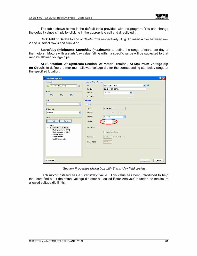
CYME 5.02 – CYMDIST Basic Analyses – Users Guide
CHAPTER 4 – MOTOR STARTING ANALYSIS 81
The table shown above is the default table provided with the program. You can change the default values simply by clicking in the appropriate cell and directly edit.
Click Add or Delete to add or delete rows respectively. E.g. To insert a row between row 2 and 3, select row 3 and click Add.
Starts/day (minimum), Starts/day (maximum): to define the range of starts per day of the motors. Motors with a starts/day value falling within a specific range will be subjected to that range’s allowed voltage dips.
At Substation, At Upstream Section, At Motor Terminal, At Maximum Voltage dip on Circuit: to define the maximum allowed voltage dip for the corresponding starts/day range at the specified location.
Section Properties dialog box with Starts /day field circled.
Each motor installed has a “Starts/day” value. This value has been introduced to help the users find out if the actual voltage dip after a ‘Locked Rotor Analysis’ is under the maximum allowed voltage dip limits.

CYME 5.02 – CYMDIST Basic Analyses – Users Guide
82 CHAPTER 4 – MOTOR STARTING ANALYSIS
4.1.3 Locked Rotor Starting Assistance Methods
Starting methods can be included in the Motor Locked Rotor Analysis. These methods are set for the motor in the Settings group box of the Properties dialog box. The types proposed include: Direct on Line, Resistor and / or Inductor, Capacitor, Auto Transformer, Star / Delta and Variable Frequency starters. (Please refer to the Equipment Reference Manual).
Note:
In the illustration above, (LRA) stands for (Locked Rotor Analysis) and (MSA) stands for dynamic (Motor Start Analysis).
4.1.4 Running and Viewing the Results of a Locked Rotor Analysis
After setting the motors status, parameters, flicker table, click Run to perform the analysis. The reports will be displayed automatically based on the Output options set at the Motors tab.
If these options were not enabled, you can generate the relevant reports via the command Report > On Calculation and selecting the desired report(s).

CYME 5.02 – CYMDIST Basic Analyses – Users Guide
CHAPTER 4 – MOTOR STARTING ANALYSIS 83
4.1.5 Locked Rotor Analysis Sample Output
The detailed report is very similar to the voltage drop complete report.

CYME 5.02 – CYMDIST Basic Analyses – Users Guide
84 CHAPTER 4 – MOTOR STARTING ANALYSIS
You can customize the report output. To do this, select the Report > On calculation menu option to display the Reports dialog box; locate your report in the list and click on the Properties hyperlink. This will display the corresponding Report Properties dialog box, where you can edit the parameters of your report. More about this can be found in the Report Menu chapter in the CYME Reference Manual.
4.1.6 Display: Color by Voltage Dip
One Line diagram color-coding
To define the color-coding used by the One Line diagram after a ‘Locked Rotor Analysis’, go to the Color Coding group box of the Display Layers Selection tab in the View > Display Options dialog box. Select the layer Voltage Dip Color (%) and click on the Modify button. These commands are also found at the Display tab of the Explorer Bar.

CYME 5.02 – CYMDIST Basic Analyses – Users Guide
CHAPTER 4 – MOTOR STARTING ANALYSIS 85
4.2 Maximum Start Size Analysis
This type of analysis is used to estimate the maximum motor size that can be started on a given section of the Network.
Select Network(s)
To select the feeder(s) or network to be considered by the analysis.
Parameters To define the value for the Maximum voltage dip allowed and the Motor kva/hp Ratio.
Options Place a check mark next to the output you want to be displayed automatically once the analysis is completed: Display the report automatically and / or Display the result box.
4.2.1 Running the Analysis and Viewing the Results
Click on Run to start the analysis. Depending on the options selected, either or both the ‘Maximum Motor Size Result Box’ and/or the ‘Maximum Start Size Analysis detail report’(s) will be displayed automatically once the analysis is complete.
The Motor Size Result Box displays the same information as the detail report but displays the information one section at a time. If there are more than one device on the section then you can select ‘S’, ‘C’, or ‘L’ to move to that device.
Hint: If you did not check the Display the result box option, generate it by running the analysis again. Un-check the detail report so you will not get double reports.
Hint: Select a section from the detailed report and both the result box and the one-line diagram will highlight the same section and vice versa.

CYME 5.02 – CYMDIST Basic Analyses – Users Guide
86 CHAPTER 4 – MOTOR STARTING ANALYSIS
The Maximum Start Size Analysis Detailed Report displays a detailed (and configurable) report on all the sections of the network.
To generate the report manually (if it was not generated automatically), or to modify the columns, use the menu command Report > On Calculation and select the desired configuration.

CYME 5.02 – CYMDIST Basic Analyses – Users Guide
CHAPTER 5 – LOAD ALLOCATION 87
Chapter 5 Load Allocation
The Load Allocation function will adjust the connected load to match the metered demand. You have two ways to define the metered demand:
• Using the Load Allocation Demand box, you may give the metered feeder demand at (or near) the substation.
• Alternatively, you may include meters to protection devices at various locations on the feeder and define the demand measured by each meter. (Refer to the Equipment Reference Manual for details concerning the Settings).
The program will assign a portion of the metered demand to each phase of each section according to the KVA (connected or actual), KWH consumed, or number of consumers connected there. (Refer to Load Settings in the Properties and Settings Chapter in the Equipment Reference Manual).
Note that the analysis takes into account motors, generators, capacitors, line susceptance and losses during the calculation. Checking the appropriate option can ignore motors and shunt capacitors.
Hint: The program can also take into account the utilization factor and the power factor you define for each load category (residential, commercial, industrial and other).

CYME 5.02 – CYMDIST Basic Analyses – Users Guide
88 CHAPTER 5 – LOAD ALLOCATION
The following are the Steps to perform a Load Allocation analysis:
Step 1 Select the appropriate network(s) in the Network and Meters group box. (If giving the Demand of the Feeder, select a downstream substation, source node or meter between the substation and the first section with a load connected to it.)
The ID of a network will appear in bold whenever demand values are associated to it and connected. Likewise, whenever a meter with non-zero values is present on a network, it will be available as a child item to the ID of the network where the meter is installed. Meters are not automatically selected to be taken into account in the calculations. Highlight the ID of a meter and enable the Connected option to include it.
Note: If there are two or more meters thus connected, then the demand measured by the meter furthest downstream is allocated to the loads on the sections downstream from it. That demand is subtracted from the demand measured by the next meter upstream from it. The difference in demand is allocated to the loads on the sections between the two meters. There should be no connected loads upstream of the meters.
Step 2 Demand: Select the Demand Type among either kVA-PF, Amp-PF, kW-PF or kW-kVAR). Enter the required data per phase. Power Factor is given in percent, not in a decimal form.
The Downstream Information group box displays the total three-phase and the per phase connected kVAs, actual kWh, consumption kWh, fixed kW and kVAR, shunt capacitor kVAR, and other relevant values related to the downstream meter or the source node. Click on the Details button to obtain the following:
You may enter a power factor of 0 % at the meter(s) if you follow Step 4. Note that the information displayed is related to the Allocation Method selected. For example, if the method selected is “Consumption kWh”, the values will be displayed in kWh rather than in kVA.
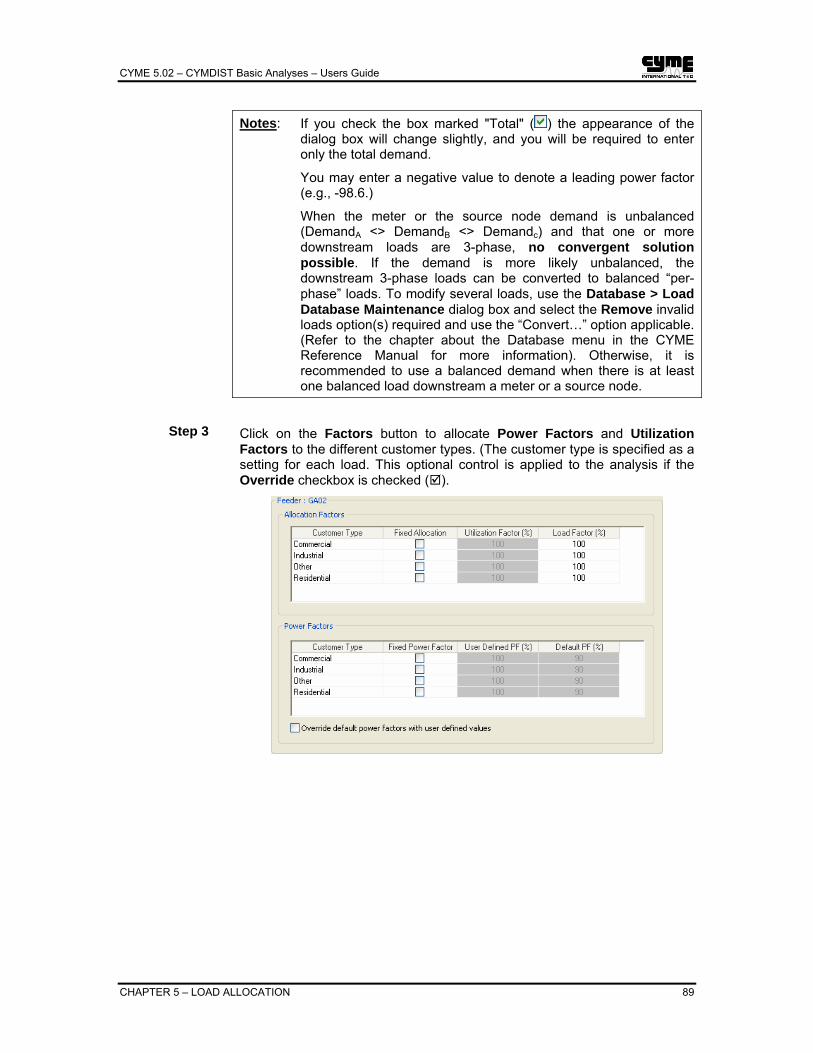
CYME 5.02 – CYMDIST Basic Analyses – Users Guide
CHAPTER 5 – LOAD ALLOCATION 89
Notes: If you check the box marked "Total" ( ) the appearance of the dialog box will change slightly, and you will be required to enter only the total demand.
You may enter a negative value to denote a leading power factor (e.g., -98.6.)
When the meter or the source node demand is unbalanced (DemandA <> DemandB <> Demandc) and that one or more downstream loads are 3-phase, no convergent solution possible. If the demand is more likely unbalanced, the downstream 3-phase loads can be converted to balanced “per-phase” loads. To modify several loads, use the Database > Load Database Maintenance dialog box and select the Remove invalid loads option(s) required and use the “Convert…” option applicable. (Refer to the chapter about the Database menu in the CYME Reference Manual for more information). Otherwise, it is recommended to use a balanced demand when there is at least one balanced load downstream a meter or a source node.
Step 3
Click on the Factors button to allocate Power Factors and Utilization Factors to the different customer types. (The customer type is specified as a setting for each load. This optional control is applied to the analysis if the Override checkbox is checked ( ).

CYME 5.02 – CYMDIST Basic Analyses – Users Guide
90 CHAPTER 5 – LOAD ALLOCATION
The utilization factors are applied to the kVA (connected or actual, see Step 6.) before allocating the demand proportionally. Doing this accounts for the fact that different types of consumers make more or less use of the capacity of the installed transformers that supply power to them.
You may define a characteristic power factor (PF) for each type of consumer (e.g., all residential loads have 90% p.f.) and set the power factor at the meter location(s) to 0.0%. CYMDIST will allocate the demand kVA, ensure the desired power factor at every load, and compute the resulting power factor at each meter.
Alternatively, you can force CYMDIST to respect the power factors at the meter location(s) by setting those and defining the characteristic power factor of all consumer types except one. The power factor of the consumer type (that is actually connected in the feeder) must be set to 0.0 to give the calculation a degree of freedom. The load allocation will find the power factor for this consumer type.
Step 4 You may select another (or more) feeder and/or meter that you wish to use as meter location(s), by repeating 2. to 4 for each of those points.
Step 5 In the Allocation Method group box, select a method to use:
• Connected kVA divides the metered demand among the loads in proportion to each one’s transformer capacity (adjusted for utilization factor, see Step 4).
• Connected kWh divides the metered demand among the loads in proportion to each one’s energy consumption.
• REA divides the metered demand among the loads according to the kWh and the number of consumers each load type represents.
• Actual kVA divides the metered demand among the loads in proportion to the kVA defined for each load. This is Useful if you keep the peak load on each section in your load database. Then, in your study, you can re-allocate the load to correspond with demand metered at some time other than peak demand.
With all of the above methods, the original load kVA is of course replaced by the new allocated value, but only within the study.
Note: Ensure that all loads have the same sort of data defined for them, be it kWH, kVA or number of consumers and kWh.
Step 6 Click on the Parameters button. Type in the Tolerance field the desired accuracy for the calculation. This information is required since the Load Allocation is an iterative Power Flow calculation. Type a value in the Initial Losses field; this is an approximation of the losses in kW and in kVAR.
In the Load Adjustments group box, if the Adjust the loads using voltage drop calculation option is checked, the loads will be adjusted to reach the target demand (s), indicated in steps 1 and 2, using the voltage drop calculations. In other words, if this option is not checked, the load allocation calculation considers only the initial losses without considering the network losses and voltage drops results provided by the voltage drop analysis. Unchecking this option facilitates a converging load allocation. It is however less rigorous. This option is checked by default.

CYME 5.02 – CYMDIST Basic Analyses – Users Guide
CHAPTER 5 – LOAD ALLOCATION 91
• The options in the Device Options group box, provides the capability to
consider or to ignore some devices in the analysis.
• The option Unlock All Fixed Loads allows to unlock all the network loads that were previously locked in order to use them in the calculations.
• The option Unlock All Initially Fixed Loads allows to unlock only the loads that are defined as Initially Locked in the Load Properties.
• The option Compute Diversity Factors of Transformers automatically computes the diversity of the demand metered at a transformer based on the total demand of metered at downstream meters connected to this transformer.
Note: If the load on certain sections is well defined, then you can protect it from being modified by the load allocation module by modifying its Status to “Locked” in the corresponding Section Properties dialog box. Spot and distributed loads may be individually protected.
The Load Allocation Module sums up the entire load which is protected by the Lock, subtracts that total from the metered demand, and allocates the remainder to the loads which are not locked. The connected KVA, KWH or customers on the section that is defined for the Locked loads are not used in the allocation.
The Options group box includes a convenient option to unlock all such fixed loads before running the Load Allocation.

CYME 5.02 – CYMDIST Basic Analyses – Users Guide
92 CHAPTER 5 – LOAD ALLOCATION
Step 7 Click on Run.
When the calculation is complete, the allocated load (kW and kVAR) are populated in the Load Properties dialog box of every section, except those where the allocated load has been defined and is being protected by the Lock option. The connected kVA, kWH or number of customers is not affected.
The “Lock” options for load allocation are found in the Settings group box of the Properties dialog box.
Note: If no solution is found within the allowed number of iterations:
• Try increasing the Maximum number of iterations or adjust your load data and try again.
• Do not specify an unbalanced demand upstream of a D-Y/ Y-D transformer.
• Try running with only 10% of the actual demand. If it still does not converge, look for abnormally high impedance or long conductor lengths.
• If using multiple metering points, try removing one meter at a time.
You may request a Load Allocation report. Use the Report > On Calculation menu command. Select Load Allocation in the Show drop-down list to see all the related reports available. Click on the Properties hyperlink adjacent to the report name to display the corresponding dialog box where you can customize the report.
5.1.1 Summary of the Connected kVA Method
Let “s” and “k” denote section and phase respectively.
)(),(_)( FactorLoadksKVAConnectedkTKVAs∑ ×=
⎥⎦
⎤⎢⎣
⎡ ××=
)()(),(_)(),(_
kTKVAFactorLoadksKVAConnectedkKWdemksAllocKW
1)(
1),(_),(_2
−⎟⎟⎠
⎞⎜⎜⎝
⎛×=
kPFksallocKWksAllocKVAR

CYME 5.02 – CYMDIST Basic Analyses – Users Guide
CHAPTER 5 – LOAD ALLOCATION 93
5.1.2 Summary of the kWH Method
Let “s” and “k” denote section and phase respectively.
)(),()( FactorLoadkskWhkTKWhs∑ ×=
⎥⎦
⎤⎢⎣
⎡ ××=
)()(),()(),(_
kTKWhFactorLoadksKWhkKWdemksAllocKW
1)(
1),(_),(_2
−⎟⎟⎠
⎞⎜⎜⎝
⎛×=
kPFksallocKWksAllocKVAR
5.1.3 Summary of Actual kVA Method
Let “s” and “k” denote section and phase respectively.
)UtilFactor(x)k,s(kVAActual)k(TKVAs∑=
1)(
1),(_),(_2
−⎟⎟⎠
⎞⎜⎜⎝
⎛×=
kPFksallocKWksAllocKVAR
5.1.4 Summary of the REA Method
[ ]40+k)(s,C4.0)kC(s,4.01k)C(s,=k)A(s, 2⋅+⋅−×
( )k)/C(s,k)kWH(s, 0.885
0.005925 =k) B(s, ×
k)B(s,k)A(s,=k)kWrea(s, ×
Where:
• kWH(s,k) is the billing kWH for section “s”, phase “k”.
• C(s,k) is the number of consumers on section “s”, phase “k”.
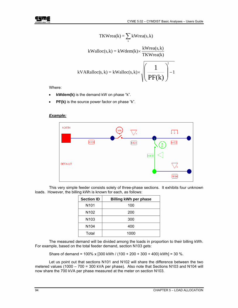
CYME 5.02 – CYMDIST Basic Analyses – Users Guide
94 CHAPTER 5 – LOAD ALLOCATION
∑s
k)kWrea(s,=TKWrea(k)
TKWrea(k)k)kWrea(s,kWdem(k)=k)kWalloc(s, ×
1k)kWalloc(s,=k)s,kVARalloc(PF(k)
12
−× ⎟⎟⎠
⎞⎜⎜⎝
⎛
Where:
• kWdem(k) is the demand kW on phase “k”.
• PF(k) is the source power factor on phase “k”.
Example:
This very simple feeder consists solely of three-phase sections. It exhibits four unknown loads. However, the billing kWh is known for each, as follows:
Section ID Billing kWh per phase N101 100
N102 200
N103 300
N104 400
Total 1000
The measured demand will be divided among the loads in proportion to their billing kWh. For example, based on the total feeder demand, section N103 gets:
Share of demand = 100% x [300 kWh / (100 + 200 + 300 + 400) kWh] = 30 %.
Let us point out that sections N101 and N102 will share the difference between the two metered values (1000 – 700 = 300 kVA per phase). Also note that Sections N103 and N104 will now share the 700 kVA per phase measured at the meter on section N103.
CYME 5.02 – CYMDIST Basic Analyses – Users Guide
CHAPTER 5 – LOAD ALLOCATION 95
This implies that section N103 share would be:
Share for N103 = 700 kVA x [300 kWh / (300 + 400) kWh] = 300 kVA per phase.
• This is the same proportion (30%) as if the total feeder demand were being divided among the loads (i.e., no meters defined, just the feeder demand at the substation).
• However, if the meter on section N103 had a reading of only 500 kVA per phase instead, then the share of the load that would be assigned to section N103 would be:
Share for N103 = 500 kVA x [300 kWh / (300 + 400) kWh] = 214.3 kVA per phase.
• This is 21.4% of the total feeder demand, down from 30%. Sections N101 and N102 would share the remaining 500 kVA (= 1000 – 500) kVA per phase.
• This little example illustrates the increased detail that is possible with multiple metering points. Note that the measured power factor could be different at each meter.


CYME 5.02 – CYMDIST Basic Analyses – Users Guide
CHAPTER 6 – LOAD BALANCING CALCULATION 97
Chapter 6 Load Balancing Calculation
The Load Balancing analysis will determine which loads can be reconnected to different phases so as to minimize kW losses or balance the current, the load, or the voltage. It reports a series of individual changes to the network and the objectives improvement with each change.
The load balancing option can be activated from the analysis menu Analysis > Load Balancing or from the Simulation toolbar.
The load flow analysis module will run a voltage drop analysis for each change made. It then retains the change that reduces the losses the most or that balances the load, the current, or the voltage the best; and repeats the whole process to find the subsequent change and so on. The process will continue until no change can further optimize the solution.
The simulation progress is displayed in a separate report window by displaying the names of the sections it is evaluating. When the calculations are complete, this window disappears and the results of the findings can be found in the Result tab of the Load Balancing Analysis dialog box or in the Load Balancing Report. These results contain which loads can be reconnected and what is the effect on the network.
Note that capacitors can affect the results of the Load Balancing analysis. You might want to try Load Balancing with all the capacitors temporarily turned off, just to compare the results. To do so select the menu command Analysis > Load Flow, go to the Controls tab, and exclude the capacitors by removing the check marks.

CYME 5.02 – CYMDIST Basic Analyses – Users Guide
98 CHAPTER 6 – LOAD BALANCING CALCULATION
6.1.1 Location Tab
The Location tab shows the main analysis window of the Load Balancing Module which allows you to define the load balancing study parameters.
Select Location(s)
Contains a tree-structured list of all locations loaded in memory that can be balanced. One or more locations in this list must be selected by clicking the appropriate check box ( ). Disconnected or open devices and 1-phase sections can’t be balanced and are not available in the list. Note: When more than one location is selected, all locations that
belong to the same network or dependant networks are optimized at the same time. Networks are dependant if they are directly connected (looped) or if they connect through other networks. For example, feeders from a same substation will be dependant only if the substation itself is loaded in memory. So, loading only the minimum networks may considerably decrease the processing time when multiple locations are selected.
Find The command Find searches and highlights an item in the tree. Type a complete or partial text string and click Find.
Objectives This group box offers four analysis objectives on which the selected locations will be evaluated. They are:
• Minimize the KW losses: minimize the total loss on all involved network.
• Balance loads (KVA): minimize the kVA unbalance factor. For a location, the factor is the highest of all phases and for each phase the factor is:

CYME 5.02 – CYMDIST Basic Analyses – Users Guide
CHAPTER 6 – LOAD BALANCING CALCULATION 99
• Balance currents: minimize the current unbalance factor. The formula for this factor is:
• Balance voltages: minimize the voltage unbalance factor.
For 3-phases locations, the formula is:
Restrictions can be used to reduce the number of steps (and the processing time) by stopping when the improvements are sufficiently small. The optimization for a location will stop if one of the restriction for the selected objective is met:
• The last step’s loss reduction in kW is lower than “Minimum kW loss reduction”;
• The reduction on all locations of the average kVA unbalance, current unbalance factor or voltage unbalance factor is lower than “Minimum kVA average unbalance”, “Minimum current unbalance factor” or “Minimum voltage unbalance factor”, respectively;
• The current (or voltage) differences on all phases of all locations are all lower than “Minimum Current” (or “Minimum Voltage”).
Restrictions You can reduce the processing time of the load balancing analysis by de-selecting ‘single-phase, ‘two-phase’ or ‘three-phase’ sections options. For example, by de-selecting three-phase sections, the program will not try at all to reconnect loads to different phases within three-phase sections. When Ignore Rephasing is checked, all sections selected in the Ignored Rephasing list won’t be considered when trying to find the best rephasing.

CYME 5.02 – CYMDIST Basic Analyses – Users Guide
100 CHAPTER 6 – LOAD BALANCING CALCULATION
Hint: When the analysis is running, if the “Stop” button is clicked, all rephasing found up to date will be kept.
6.1.2 Display Tab
To define the colors and the content of the rephasing information tag that will be displayed in the one line diagram after a load balancing analysis.
Tag Applied rephasing (and Unapplied rephasing): to select text, background and border colors, click on the down arrow to unfold the color palette.
Hint: Use different sets of colors to distinguish between the applied and unapplied rephasing tags.
Tag Information, click to mark the checkbox for the information you want to display. Uncheck those you do not want to appear.
Display the load balancing report will automatically display the report when the dialog is closed if the analysis completed successfully. It’s the same report that can be manually selected in the Reports dialog.
The iteration report display all rephasing tested during the analysis and the result of each step.

CYME 5.02 – CYMDIST Basic Analyses – Users Guide
CHAPTER 6 – LOAD BALANCING CALCULATION 101
6.1.3 Result Tab
Once the analysis is completed, the Result tab of the Load Balancing dialog box will be filled automatically. It will show you which loads to reconnect to different phases so as to meet the objective you have selected. It reports a series of individual changes (steps) and the kW reduction due to each change.
Balancing Locations displays the results (if any) in a tree structure list and in order of recommended operation, (step 1, step 2, … step N).
The first level of the tree is network groups and they are simply numbered. All locations in these networks have rephasing that can impact other locations in the group. The reports are separated the same way and the list of networks in each group is displayed in these reports.
Click on each recommended rephasing step to see the changes and the result each will have on the target location. To apply a specific step, select it in the list and click the Apply button; once applied, the name of the step will appear in boldface.
Hint: Right click in the ‘Balancing location’ frame to access a context sensitive menu where you can perform a ‘Apply’ and or ‘Undo’ operations.

CYME 5.02 – CYMDIST Basic Analyses – Users Guide
102 CHAPTER 6 – LOAD BALANCING CALCULATION
6.1.4 Load Balancing Report
To view the load balancing report, select the menu command Report > On calculation.
Sample Load Balancing Report (Spreadsheet)
Location summary column definitions:
• Ineutral (A): The neutral current at the location.
• Total Losses (KW): Indicates the total losses at the location that could be obtained by the recommended rephasing.
• Average KVA Unbal.: Indicates the average kVA unbalanced percentage at the location.
• Current Unbal. Factor: Indicates the unbalanced current factor percentage at the location.
• Voltage Unbal. Factor: Indicates the unbalanced voltage factor percentage at the location.
Hint: Alternately, based on the report information, you can use the Edit > Reconfigure sections command to implement the recommended changes.

CYME 5.02 – CYMDIST Basic Analyses – Users Guide
CHAPTER 6 – LOAD BALANCING CALCULATION 103
The Recommended Rephasing section of the report displays results as was reported in the Result tab.
The report options are available in the Reports dialog when clicking on Properties :
Include all networks in the same report determine if one report is created for all
locations or if one is created for each network group as defined in the Result tab.
If Only display reports that includes rephasing is checked, reports that don’t contain any recommended rephasing won’t be displayed.
Report Mode allows selecting the destination of the report: Excel or report tab in CYME.
These options are used if the reports are displayed because Display the load balancing report is checked in the Display tab.

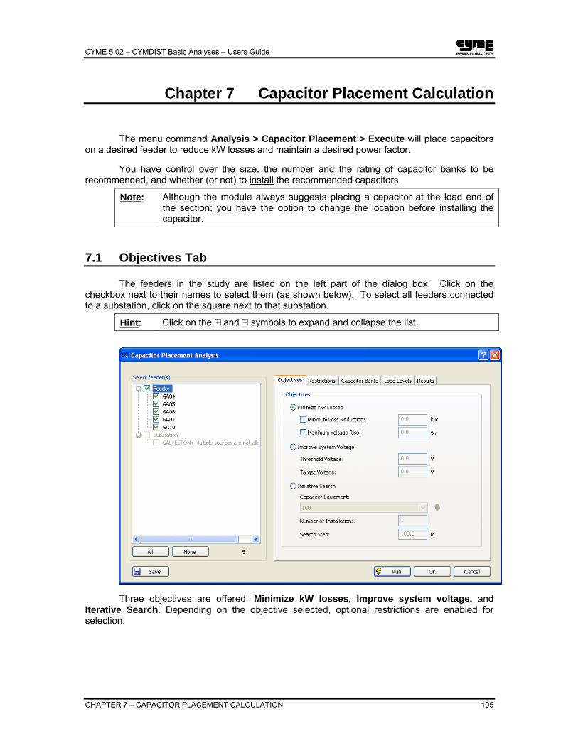
CYME 5.02 – CYMDIST Basic Analyses – Users Guide
CHAPTER 7 – CAPACITOR PLACEMENT CALCULATION 105
Chapter 7 Capacitor Placement Calculation
The menu command Analysis > Capacitor Placement > Execute will place capacitors on a desired feeder to reduce kW losses and maintain a desired power factor.
You have control over the size, the number and the rating of capacitor banks to be recommended, and whether (or not) to install the recommended capacitors.
Note: Although the module always suggests placing a capacitor at the load end of the section; you have the option to change the location before installing the capacitor.
7.1 Objectives Tab
The feeders in the study are listed on the left part of the dialog box. Click on the checkbox next to their names to select them (as shown below). To select all feeders connected to a substation, click on the square next to that substation.
Hint: Click on the and symbols to expand and collapse the list.
Three objectives are offered: Minimize kW losses, Improve system voltage, and Iterative Search. Depending on the objective selected, optional restrictions are enabled for selection.
CYME 5.02 – CYMDIST Basic Analyses – Users Guide
106 CHAPTER 7 – CAPACITOR PLACEMENT CALCULATION
Minimize kW losses provides the following options:
• Minimum loss reduction allows you to prevent the analysis from suggesting capacitors that do not reduce losses by at least this amount.
• Maximum voltage rise allows you to prevent the analysis from suggesting capacitors that would cause the voltage to rise too much when they are connected.
% 100
VVVDeviation % . × −
= without
withoutcapacitorwith
Improve system voltage allows you to define:
• Threshold voltage, below which the voltage is “unacceptable”
• Target voltage which is the voltage CYMDIST will try to obtain at every initially “unacceptable” location.
Iterative Search is used to find an exhaustive list of all possible capacitor placement solutions. Both objectives to minimize kW losses and improve the system voltage apply. Looped networks with unbalanced operating voltages are also taken into account by this method. Specify:
• Capacitor Equipment is the capacitor defined in the Equipment database that is to be used
• Number of Installations is the desired number of the capacitor selected to be installed in the network
• Search Step specifies a distance at which the possibility of installing a capacitor is to be examined. If the user specifies 500m, then the analysis will only analyze the possibility to add a capacitor at every 500m. Should the user wishes to take into account all sections in the network, input 0.
7.2 Restrictions Tab
Depending on the objective selected, additional constraints will be enabled for selection. The additional restrictions one can apply are:
• Minimum distance from substation sets the minimum distance away from the substation for the installation of a capacitor.
• Minimum distance between capacitors • Maximum Power factor at the capacitor location. • Maximum fault current prevents installation where the fault level is too high. • Overcompensation Limit • Apply Loading/Voltage Limits as defined in the Load Flow analysis.
You may prevent CYMDIST from suggesting capacitors for certain locations as well. If so, in the Ignored Sections block, choose to ignore underground sections, single-phase, two-phase and/or three-phase lines.

CYME 5.02 – CYMDIST Basic Analyses – Users Guide
CHAPTER 7 – CAPACITOR PLACEMENT CALCULATION 107
Enable Ignore Specific locations to eliminate specific sections from consideration. Click on the Edit button and choose the sections from the pop up dialog box.
7.3 Capacitor Banks Tab
You may specify the capacitor(s) to be used from the equipments in the Equipment Database when select the option Select from the Equipment database. That is, use only certain standard capacitor types. Select which of the types of capacitors are to be installed. (Click to select )

CYME 5.02 – CYMDIST Basic Analyses – Users Guide
108 CHAPTER 7 – CAPACITOR PLACEMENT CALCULATION
The Install in this order option forces CYMDIST to use up the specified quantity of each selected type before installing any of the next type from top to bottom in the list. (This is optional.) If the option is not checked, CYMDIST will select the ones that give the best results.
Change the order by selecting a type and clicking Move Up or Move down. Enter the
quantity for the selected type at the bottom and click on the button.
You may include or ignore all capacitor banks that are already in service.
Hint: You can disregard specific capacitors by disconnecting them temporarily - before performing a capacitor placement calculation. See the Section Properties dialog box (double-click on the section on the one-line to display it).
When the option Select from the Equipment database is not selected, you may then specify restrictions on the size and number of capacitor banks. Specify:
• Minimum capacitor bank size that will justify an installation. • Maximum capacitor bank size that can be installed in one location. • Increment capacitor bank size that may be added to a capacitor bank. (If you do
not activate this option, then the increment size is the same as the minimum size.) • Number of installation(s) per feeder, to limit the number of separate capacitors.
You can also choose to ignore existing capacitor banks here as well.

CYME 5.02 – CYMDIST Basic Analyses – Users Guide
CHAPTER 7 – CAPACITOR PLACEMENT CALCULATION 109
7.4 Load Levels Tab
The purpose of this set of parameters is to help CYMDIST decide which of the recommended capacitors should be fixed (manual) and which should be switched by automatic controls. Sometimes it will suggest a combination.
You may define up to three loading levels. For each level, define a global multiplier (Loading) for all loads on the feeder, a Power Factor desired at the substation and the portion of the year (Time at Loading) for which this condition applies.
Hint: Enter Time at loading = 0 for any load condition you do not want to define.
The sum of the “Times at loading” must equal 100%.
CYMDIST optimizes the capacitor placement for the condition that applies for the longest time first (usually Normal load). It then optimizes for the other conditions. Any recommended capacitor that is not needed at a lighter load condition will be recommended as ‘switched’, as will any additional capacitors needed at a heavier load condition. The others will be recommended as ‘fixed’ (manually controlled).
Hint: Enter a negative value (e.g., -99%) to define a P.F. Any additional capacitor required to correct the P.F. at the substation beyond 100% will be reported as an amount of kVAR to be installed at the substation.
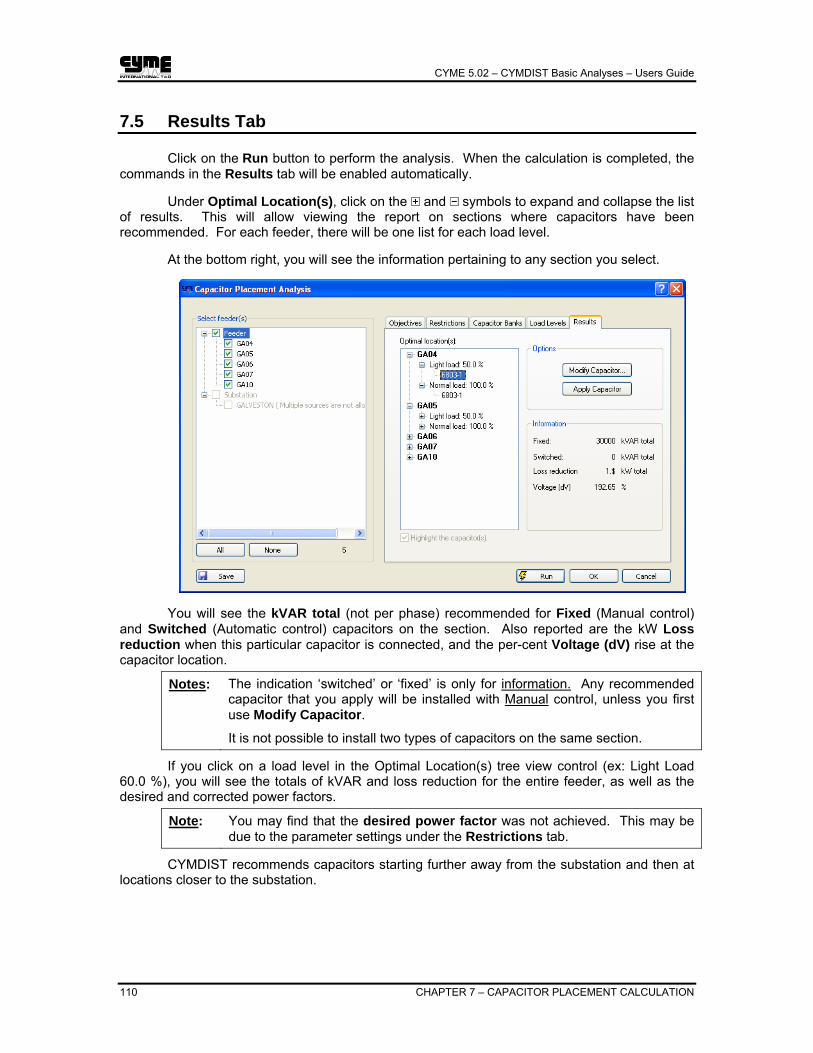
CYME 5.02 – CYMDIST Basic Analyses – Users Guide
110 CHAPTER 7 – CAPACITOR PLACEMENT CALCULATION
7.5 Results Tab
Click on the Run button to perform the analysis. When the calculation is completed, the commands in the Results tab will be enabled automatically.
Under Optimal Location(s), click on the and symbols to expand and collapse the list of results. This will allow viewing the report on sections where capacitors have been recommended. For each feeder, there will be one list for each load level.
At the bottom right, you will see the information pertaining to any section you select.
You will see the kVAR total (not per phase) recommended for Fixed (Manual control) and Switched (Automatic control) capacitors on the section. Also reported are the kW Loss reduction when this particular capacitor is connected, and the per-cent Voltage (dV) rise at the capacitor location.
Notes: The indication ‘switched’ or ‘fixed’ is only for information. Any recommended capacitor that you apply will be installed with Manual control, unless you first use Modify Capacitor.
It is not possible to install two types of capacitors on the same section.
If you click on a load level in the Optimal Location(s) tree view control (ex: Light Load 60.0 %), you will see the totals of kVAR and loss reduction for the entire feeder, as well as the desired and corrected power factors.
Note: You may find that the desired power factor was not achieved. This may be due to the parameter settings under the Restrictions tab.
CYMDIST recommends capacitors starting further away from the substation and then at locations closer to the substation.
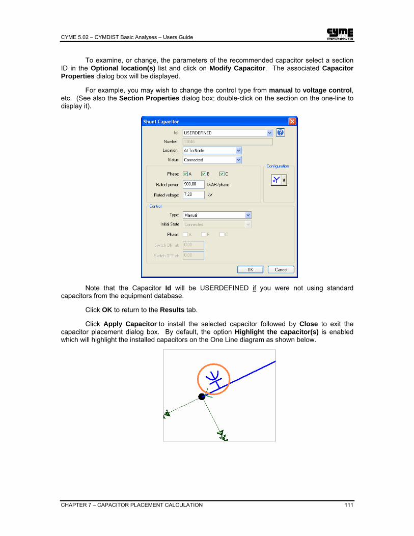
CYME 5.02 – CYMDIST Basic Analyses – Users Guide
CHAPTER 7 – CAPACITOR PLACEMENT CALCULATION 111
To examine, or change, the parameters of the recommended capacitor select a section ID in the Optional location(s) list and click on Modify Capacitor. The associated Capacitor Properties dialog box will be displayed.
For example, you may wish to change the control type from manual to voltage control, etc. (See also the Section Properties dialog box; double-click on the section on the one-line to display it).
Note that the Capacitor Id will be USERDEFINED if you were not using standard capacitors from the equipment database.
Click OK to return to the Results tab.
Click Apply Capacitor to install the selected capacitor followed by Close to exit the capacitor placement dialog box. By default, the option Highlight the capacitor(s) is enabled which will highlight the installed capacitors on the One Line diagram as shown below.
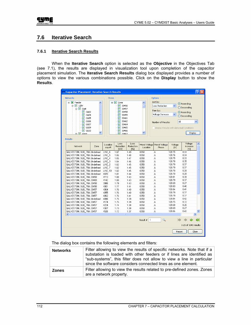
CYME 5.02 – CYMDIST Basic Analyses – Users Guide
112 CHAPTER 7 – CAPACITOR PLACEMENT CALCULATION
7.6 Iterative Search
7.6.1 Iterative Search Results
When the Iterative Search option is selected as the Objective in the Objectives Tab (see 7.1), the results are displayed in visualization tool upon completion of the capacitor placement simulation. The Iterative Search Results dialog box displayed provides a number of options to view the various combinations possible. Click on the Display button to show the Results.
The dialog box contains the following elements and filters:
Networks Filter allowing to view the results of specific networks. Note that if a substation is loaded with other feeders or if lines are identified as “sub-systems”, this filter does not allow to view a line in particular since the software considers connected lines as one element.
Zones Filter allowing to view the results related to pre-defined zones. Zones are a network property.
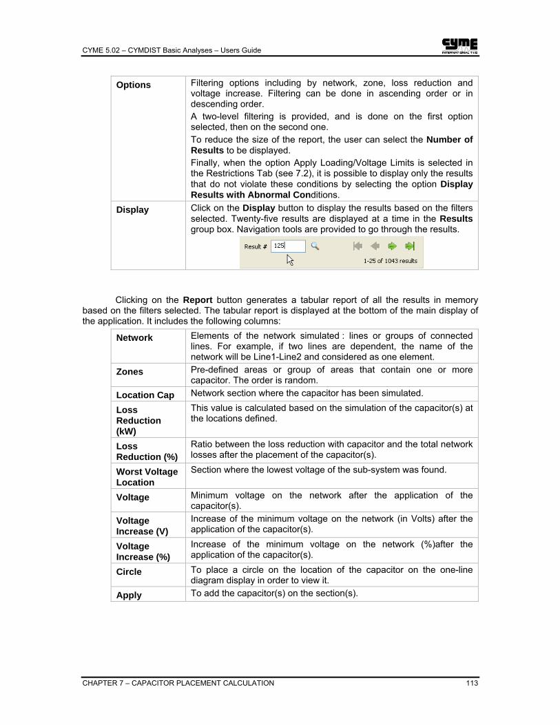
CYME 5.02 – CYMDIST Basic Analyses – Users Guide
CHAPTER 7 – CAPACITOR PLACEMENT CALCULATION 113
Options Filtering options including by network, zone, loss reduction and voltage increase. Filtering can be done in ascending order or in descending order. A two-level filtering is provided, and is done on the first option selected, then on the second one. To reduce the size of the report, the user can select the Number of Results to be displayed. Finally, when the option Apply Loading/Voltage Limits is selected in the Restrictions Tab (see 7.2), it is possible to display only the results that do not violate these conditions by selecting the option Display Results with Abnormal Conditions.
Display Click on the Display button to display the results based on the filters selected. Twenty-five results are displayed at a time in the Results group box. Navigation tools are provided to go through the results.
Clicking on the Report button generates a tabular report of all the results in memory based on the filters selected. The tabular report is displayed at the bottom of the main display of the application. It includes the following columns:
Network Elements of the network simulated : lines or groups of connected lines. For example, if two lines are dependent, the name of the network will be Line1-Line2 and considered as one element.
Zones Pre-defined areas or group of areas that contain one or more capacitor. The order is random.
Location Cap Network section where the capacitor has been simulated.
Loss Reduction (kW)
This value is calculated based on the simulation of the capacitor(s) at the locations defined.
Loss Reduction (%)
Ratio between the loss reduction with capacitor and the total network losses after the placement of the capacitor(s).
Worst Voltage Location
Section where the lowest voltage of the sub-system was found.
Voltage Minimum voltage on the network after the application of the capacitor(s).
Voltage Increase (V)
Increase of the minimum voltage on the network (in Volts) after the application of the capacitor(s).
Voltage Increase (%)
Increase of the minimum voltage on the network (%)after the application of the capacitor(s).
Circle To place a circle on the location of the capacitor on the one-line diagram display in order to view it.
Apply To add the capacitor(s) on the section(s).

CYME 5.02 – CYMDIST Basic Analyses – Users Guide
114 CHAPTER 7 – CAPACITOR PLACEMENT CALCULATION
Note: It is possible to display several reports by changing some of the filters’ parameters and clicking on the Report button to generate a report. For example, a report can be created with the results filtered in ascending order. Then, the results can be filtered by zones and a second report created and displayed in a second tab in the report pane below the main display of the application.
7.6.2 Iterative Search Color Coding
When the Iterative Search option is selected as the Objective in the Objectives Tab (see 7.1), the results can be displayed by coloring the locations on the one-line display.
Each section where the placement of a capacitor was attempted is allocated a color that corresponds to the Loss Reduction or to the Voltage Increase when the capacitor was placed on that section.
To obtain a dynamic coloring, activate the Use Auto-Scaling checkbox. Note that the
coloring will be applied to sections where only one capacitor is installed. In the case where there are more, the section will not be colored.
CYME 5.02 – CYMDIST Basic Analyses – Users Guide
INDEX 115
Index
Actual kVA Method ....................................93
ANSI Parameters Tab ...............................47
ANSI Short-Circuit Analysis.......................46
Asymmetry Factor .....................................41
Calculation Methods ..............................3, 13
Calculation Options .....................................3
Capacitor Banks Tab ...............................107
Capacitor Placement Calculation ............105
Charts ..................................................29, 63
Connected kVA Method.............................92
Controls Tab ..............................................18
Conventional Short-Circuit Analysis ..........38
Convergence Issues..................................32
Convergence Parameters ...........................3
Display Tab..............................................100
Display: Color by Voltage Dip....................84
Double-Line-to-Ground Fault.....................40
DUTY Type................................................48
Exponent Model.........................................11
Fast-Decoupled .........................................16
Fault Analysis ............................................65
Fault Current Type.....................................54
Fault Locator Analysis ...............................75
Fault Parameters Tab................................39
Fault Types ................................................39
Flicker Table ..............................................80
Gauss-Seidel .............................................14
Gauss-Seidel, Fast Decoupled and Newton-Raphson Methods..................................33
IEC Default R/X Ratios and Impedance Correction Factors .................................55
IEC Parameters Tab..................................53
IEC Short-Circuit Analysis .........................52
Include Contributions From .......................50
Iterative Search....................................... 112
Iterative Search Color Coding ................ 114
Iterative Search Results.......................... 112
kWH Method ............................................. 93
Line-to-Line Fault ...................................... 41
List of Motors and Parameters ................. 79
Load Allocation ......................................... 87
Load and Generation Scaling Factors ........ 4
Load Balancing Calculation ...................... 97
Load Balancing Report ........................... 102
Load Flow Analysis..................................... 1
Load Levels Tab ..................................... 109
Loading / Voltage Limits Tab .................... 19
Location Tab ............................................. 98
Locked Rotor Analysis Sample Output..... 83
Locked Rotor Motor Start Analysis ........... 79
Locked Rotor Starting Assistance Methods.............................................................. 82
Machine Status ......................................... 57
Maximum Start Size Analysis ................... 85
Mixed: ZIP and Exponent Model............... 11
Motor Starting Analysis............................. 79
Network Fault Analysis ............................. 70
Networks Tab............................................ 17
Networks with Abnormal Voltages............ 34
Newton-Raphson ...................................... 15
Objectives Tab........................................ 105
One-Line Diagram Coloring................ 31, 64
One-Line Diagram Tags ........................... 30
Other Calculation Parameters .................. 42
Output Tab ........................ 21, 45, 51, 59, 68
Parallel Operation of Generators.............. 35
Parameters Tab .................. 2, 66, 70, 73, 76
Peak Factor............................................... 42
CYME 5.02 – CYMDIST Basic Analyses – Users Guide
116 INDEX
REA Method ..............................................93
Report by Individual Section................27, 61
Report Tags...............................................64
Reports ................................................25, 60
Restrictions Tab.......................................106
Result Tab ...............................................101
Results.............................. 25, 60, 71, 74, 77
Results Tab..............................................110
Running and Viewing the Results of a Locked Rotor Analysis ...........................82
Running the Analysis and Viewing the Results ...................................................85
Short-Circuit Analysis ............................... 37
Shunt Fault Analysis ................................. 65
Shunt Fault Results .................................. 69
Single-Line-to-Ground Fault ..................... 41
Solving the Load Flow .............................. 23
Three-phase Fault .................................... 39
Voltage and Frequency Sensitivity Load Model....................................................... 8
Voltage Drop Calculation Technique ........ 13
Voltage Drop Method................................ 32
Voltage Sag Analysis................................ 73
ZIP Model.................................................. 10