DATA 8Spring 2018

Slides created by John DeNero (denero@berkeley.edu) and Ani Adhikari (adhikari@berkeley.edu)

Lecture 39Part I: Health Case Study

Announcements

Diet Experiment: Review

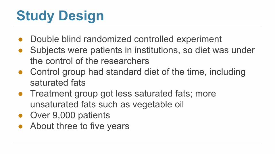
Study Design● Double blind randomized controlled experiment● Subjects were patients in institutions, so diet was under

the control of the researchers● Control group had standard diet of the time, including

saturated fats● Treatment group got less saturated fats; more

unsaturated fats such as vegetable oil● Over 9,000 patients ● About three to five years

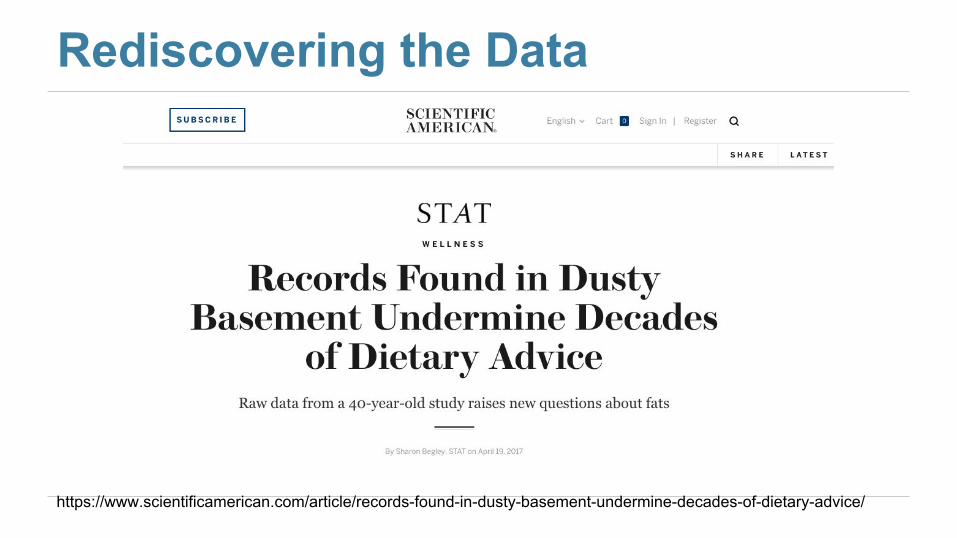
Rediscovering the Data

https://www.scientificamerican.com/article/records-found-in-dusty-basement-undermine-decades-of-dietary-advice/

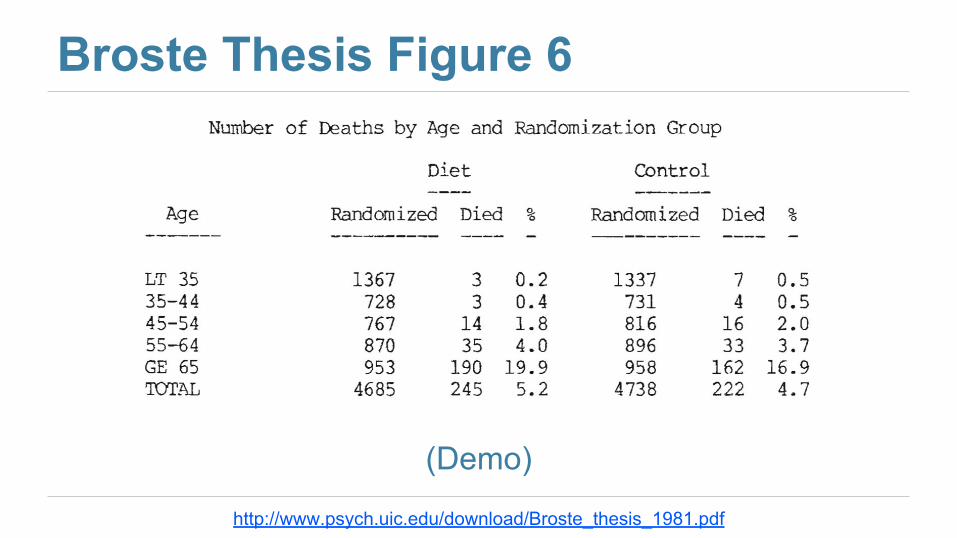
Broste Thesis Figure 6

(Demo)

http://www.psych.uic.edu/download/Broste_thesis_1981.pdf

Conclusion● Malcolm Gladwell and Robert Frantz● Revisionist History: The Basement Tapes● 00:24:30 to 00:27:47

● http://revisionisthistory.com/episodes/20-the-basement-tapes

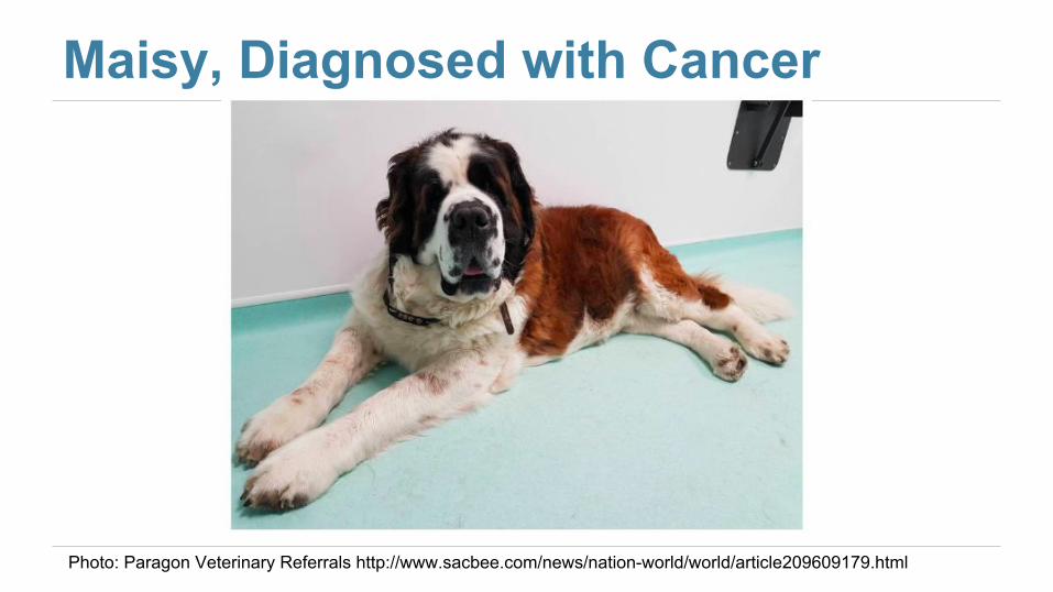
Maisy, Diagnosed with Cancer

Photo: Paragon Veterinary Referrals http://www.sacbee.com/news/nation-world/world/article209609179.html

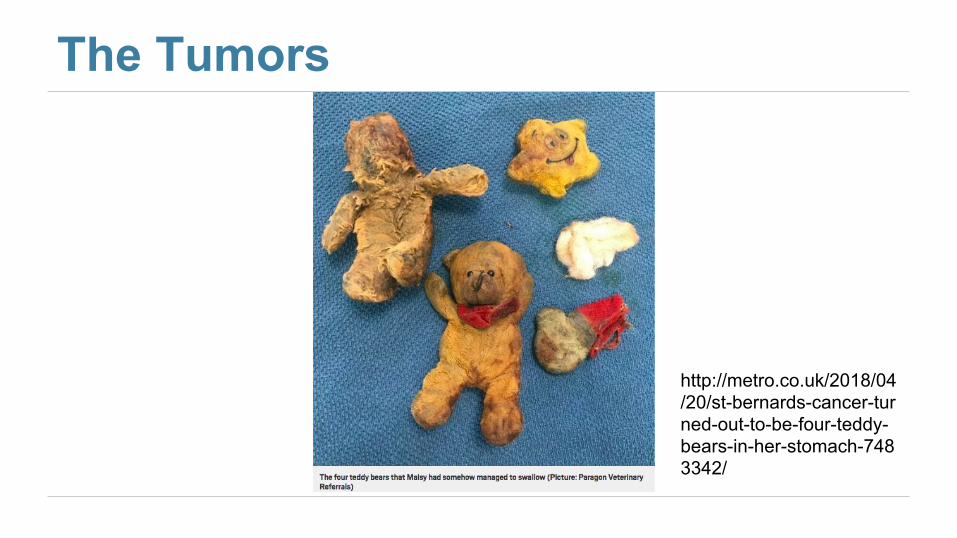
The Tumors

http://metro.co.uk/2018/04/20/st-bernards-cancer-turned-out-to-be-four-teddy-bears-in-her-stomach-7483342/

DATA 8Spring 2018

Slides created by John DeNero (denero@berkeley.edu) and Ani Adhikari (adhikari@berkeley.edu)

Lecture 39Part II: Review

DATA 8Fall 2016

Slides created by Ani Adhikari and John DeNero

Review I, December 5 Inference

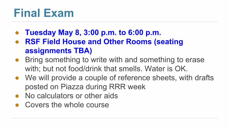
Final Exam● Tuesday May 8, 3:00 p.m. to 6:00 p.m.● RSF Field House and Other Rooms (seating

assignments TBA)● Bring something to write with and something to erase

with; but not food/drink that smells. Water is OK.● We will provide a couple of reference sheets, with drafts

posted on Piazza during RRR week● No calculators or other aids● Covers the whole course

Big Picture of Course Contents1. Python

2. Describing data

3. General concepts of inference

4. Theory of probability and statistics

5. Methods of inference

1. Python● Textbook sections

○ General features and Table methods: 3.1 - 9.3, 17.3○ sample_proportions: 11.1○ percentile: 13.1○ np.average, np.mean, np.std: 14.1, 14.2○ minimize: 15.4

2. Describing Data● Tables: Chapter 6

● Classifying and cross-classifying: 8.2, 8.3

● Visualizing Distributions: Chapter 7

● Center and spread: 14.1-14.3

● Linear trend and non-linear patterns: 8.1, Chapter 15

3. General Concepts of Inference● Study, experiment, treatment, control, confounding,

randomization, causation, association: Chapter 2● Distribution: 7.1, 7.2● Sampling, probability sample: 10.0● Probability distribution, empirical distribution, law of

averages: Chapter 10● Population, sample, parameter, statistic, estimate: 10.1,

10.3● Model: every null and alternative hypothesis; 16.1

4. Probability and Statistics: Theory ● Descriptive statistics:

○ One variable (average, SD, etc)○ Two variables (correlation and regression)

● Probability theory:○ Exact calculations○ Normal approximation for mean of large random

sample○ Accuracy and sample size

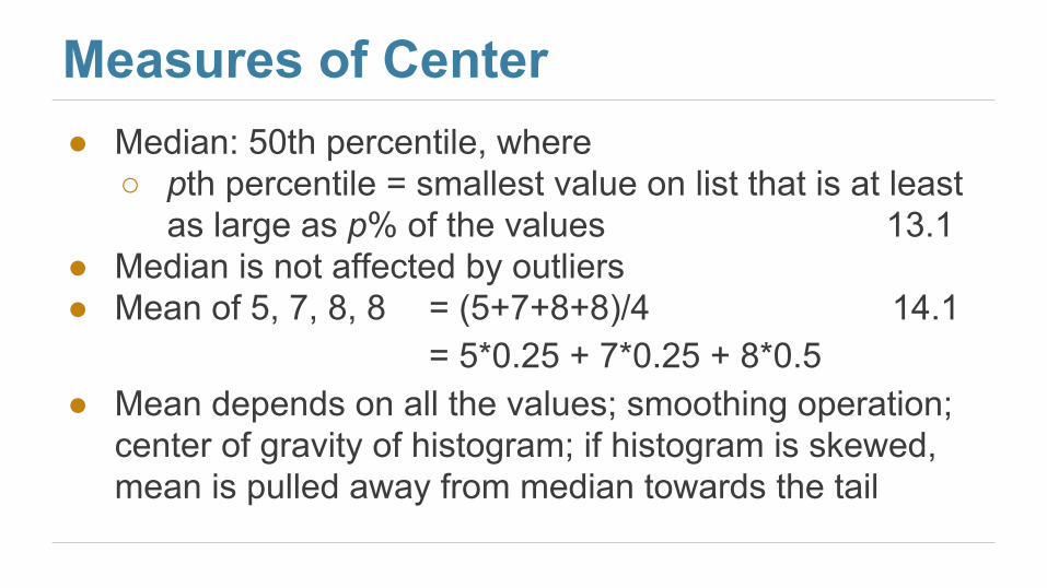
Measures of Center● Median: 50th percentile, where

○ pth percentile = smallest value on list that is at least as large as p% of the values 13.1

● Median is not affected by outliers● Mean of 5, 7, 8, 8 = (5+7+8+8)/4 14.1

= 5*0.25 + 7*0.25 + 8*0.5● Mean depends on all the values; smoothing operation;

center of gravity of histogram; if histogram is skewed, mean is pulled away from median towards the tail

Measure of Spread

root5

mean4

square of3

deviations from2

average1

Standard deviation (SD) =

Measures roughly how far off the values are from average

● 14.2

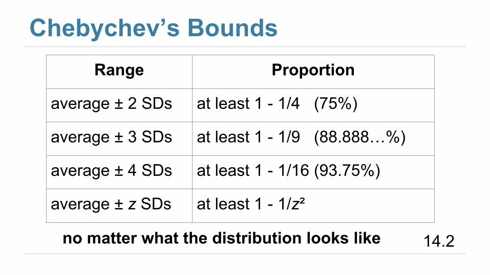
Chebychev’s BoundsRange Proportion

average ± 2 SDs at least 1 - 1/4 (75%)

average ± 3 SDs at least 1 - 1/9 (88.888…%)

average ± 4 SDs at least 1 - 1/16 (93.75%)

average ± z SDs at least 1 - 1/z²

no matter what the distribution looks like 14.2

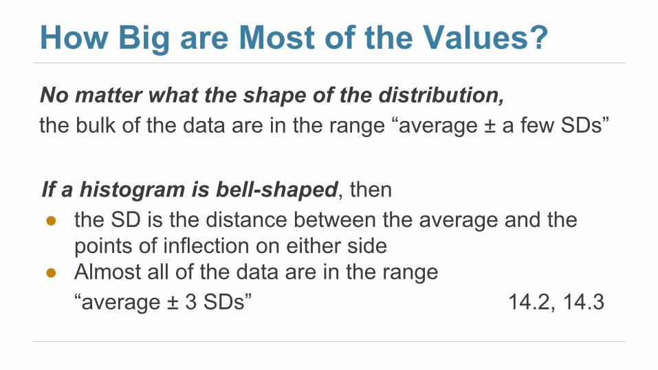
How Big are Most of the Values?No matter what the shape of the distribution,the bulk of the data are in the range “average ± a few SDs”

If a histogram is bell-shaped, then● the SD is the distance between the average and the

points of inflection on either side● Almost all of the data are in the range

“average ± 3 SDs” 14.2, 14.3

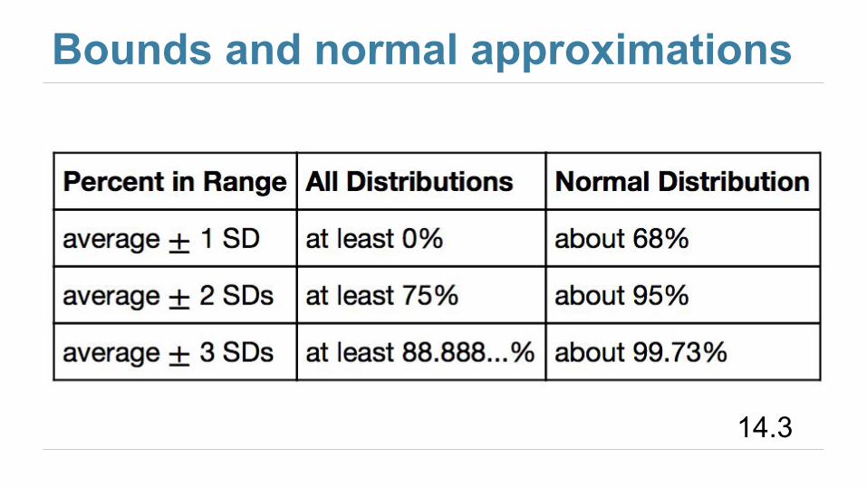
Bounds and normal approximations

14.3

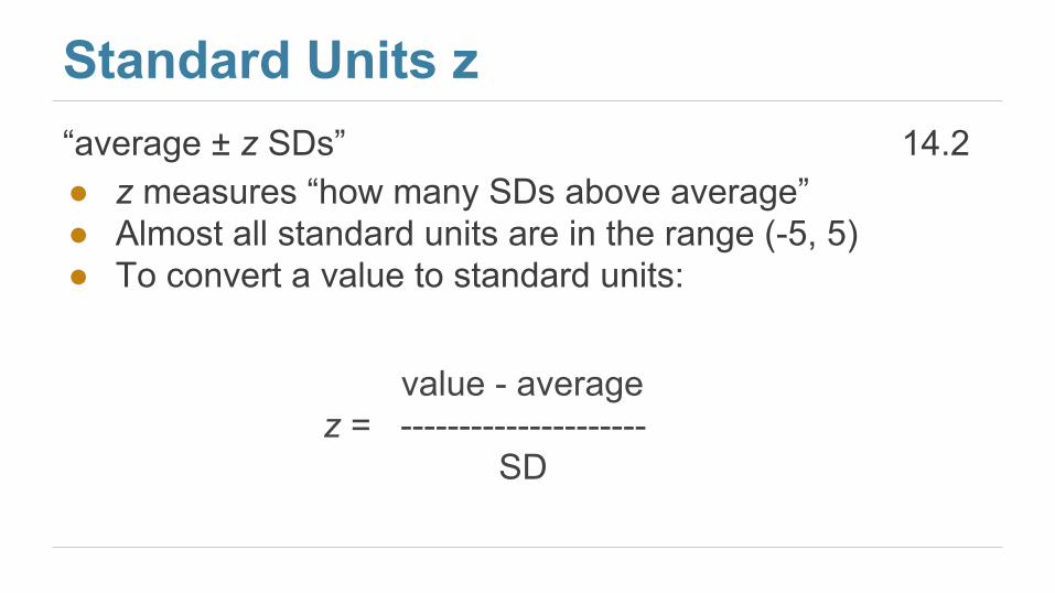
Standard Units z“average ± z SDs” 14.2● z measures “how many SDs above average”● Almost all standard units are in the range (-5, 5)● To convert a value to standard units:

value - averagez = --------------------- SD

Definition of r

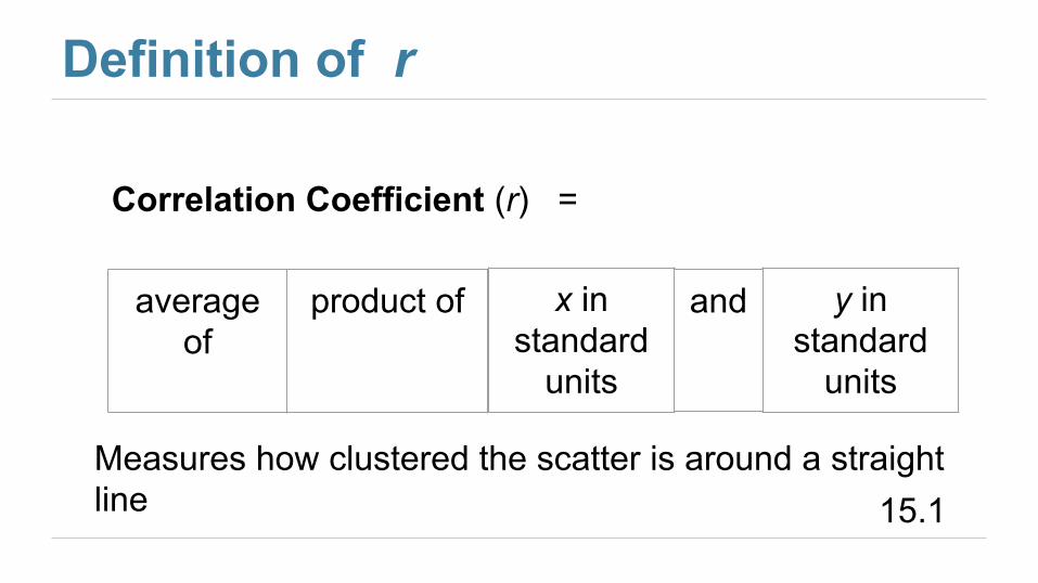
average of

product of x in standard

units

and y in standard

units

Correlation Coefficient (r) =

Measures how clustered the scatter is around a straight line 15.1

The Correlation Coefficient r● Measures linear association● Based on standard units; pure number with no units● r is not affected by changing units of measurement● -1 ≤ r ≤ 1● r = 0: No linear association; uncorrelated● r is not affected by switching the horizontal and vertical

axes● Be careful before you use it● 15.1

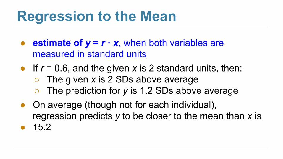
Regression to the Mean

● estimate of y = r · x, when both variables are measured in standard units

● If r = 0.6, and the given x is 2 standard units, then:○ The given x is 2 SDs above average○ The prediction for y is 1.2 SDs above average

● On average (though not for each individual), regression predicts y to be closer to the mean than x is

● 15.2

A course has a midterm (average 70; standard deviation 10)and a really hard final (average 50; standard deviation 12)

If the scatter of midterm & final scores for students looks like a typical oval with correlation 0.75, then...

What do you expect the average final score would be for

Regression Estimate, Method I

a student who scored 90 on the midterm?2 standard units on midterm,so estimate 0.75 * 2 = 1.5 standard units on final. So estimated final score = 1.5 * 12 + 50 = 68 points

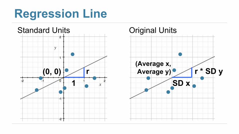
Regression LineStandard Units

(0, 0)1

r

Original Units

(Average x, Average y)

SD xr * SD y

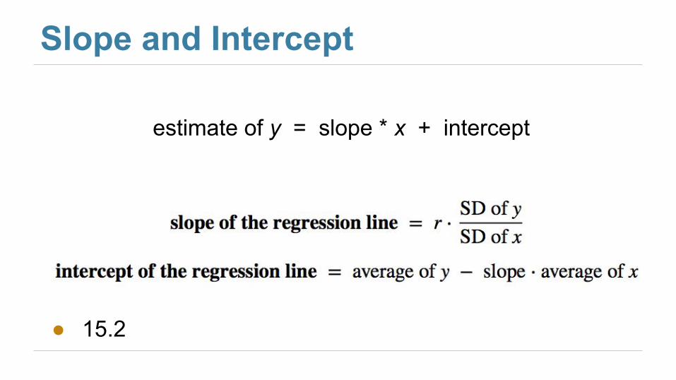
Slope and Intercept

estimate of y = slope * x + intercept

● 15.2

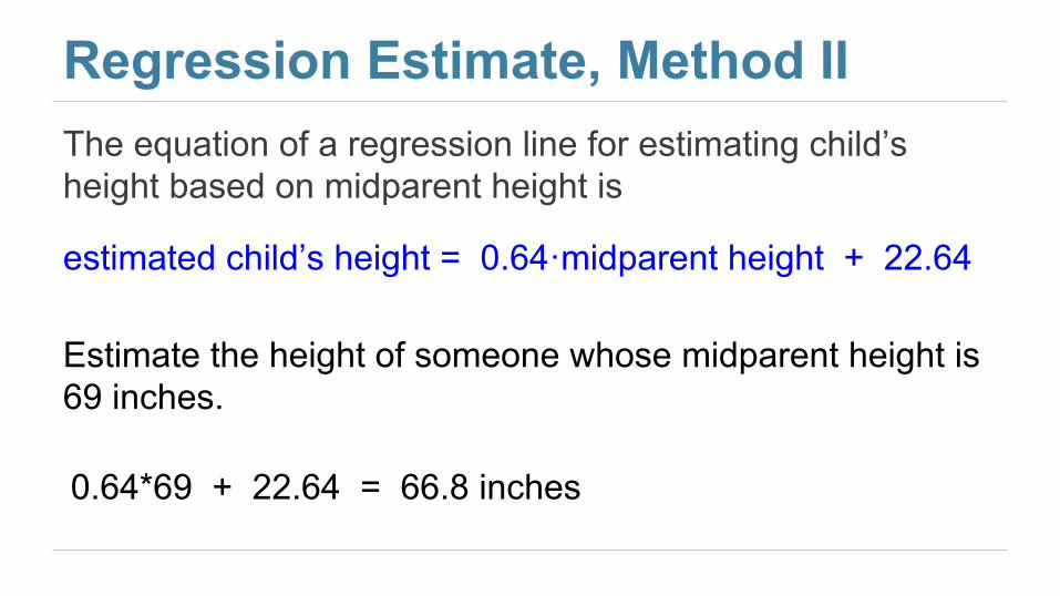
Regression Estimate, Method IIThe equation of a regression line for estimating child’s height based on midparent height is

estimated child’s height = 0.64·midparent height + 22.64

Estimate the height of someone whose midparent height is 69 inches.

0.64*69 + 22.64 = 66.8 inches

Least Squares● Regression line is the “least squares” line● Minimizes the root mean squared error of prediction,

among all possible lines● No matter what the shape of the scatter plot, there is

one best straight line○ but you shouldn’t use it if the scatter isn’t linear

● 15.3, 15.4

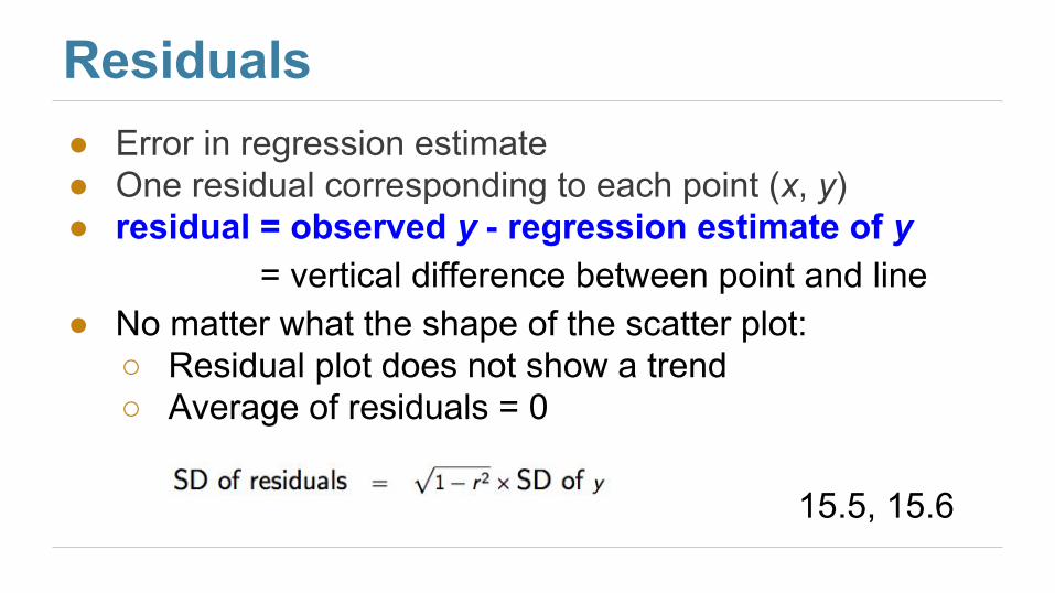
Residuals● Error in regression estimate● One residual corresponding to each point (x, y)● residual = observed y - regression estimate of y

= vertical difference between point and line ● No matter what the shape of the scatter plot:

○ Residual plot does not show a trend○ Average of residuals = 0

15.5, 15.6

Equally Likely Outcomes● If all outcomes are assumed equally likely, then

probabilities are proportions of outcomes:

number of outcomes that make A happenP(A) = --------------------------------------------------------------- total number of outcomes = proportion of outcomes that make A happen● 9.5

Probability: Exact Calculations ● Probabilities are between 0 (impossible) and 1 (certain)

● P(event happens) = 1 - P(the event doesn’t happen)

● Chance that two events A and B both happen= P(A happens) x P(B happens given that A has happened)

● If event A can happen in exactly one of two ways, thenP(A) = P(first way) + P(second way)

● 9.5

Updating Probabilities● Start with prior probabilities of two classes; priors can

be subjective● Known: likelihood of data, given each of the classes

● Acquire data according to these likelihoods

● Update the prior probabilities by finding posterior probabilities of the two classes, given the data

● Tree diagrams and Bayes’ Rule: 18.1, 18.2

Large Sample Approximation: CLT Central Limit Theorem

If the sample is● large, and● drawn at random with replacement,

Then, regardless of the distribution of the population,

the probability distribution of the sample sum (or of the sample mean) is roughly bell-shaped 14.4

Random Sample Mean● Fix a sample size● Draw all possible random samples of that size● Compute the mean of each sample● You’ll end up with a lot of means● The distribution of those is the probability distribution of

the sample mean● It’s centered at the population mean● SD = (population SD)/√(sample size) 14.5● If the sample is large, it’s roughly bell shaped by CLT

Accuracy of Random Sample Mean ● Greater if SD of sample mean is smaller● Doesn’t depend on population size● Increases as sample size increases, because SD of

sample mean decreases● For 3 times the accuracy, you have to multiply the

sample size by a factor of 3² = 9● Square Root Law: If you multiply sample size by a

factor, accuracy goes up by the square root of the factor● 14.5

Application to Proportions● Fact: SD of 0-1 population ≤ 0.5 14.6 ● Total width of 95% CI for population proportion:

= 4 SDs of the sample proportion= 4 x (SD of 0-1 population)/√(sample size)

≤ 4 x 0.5/√(sample size)= 2 / √(sample size)

● So if you know the desired width of the interval, you can solve for (an overestimate of) the sample size

5. Methods of Inference

● Making conclusions about unknown features of the population or model, based on assumptions of randomness

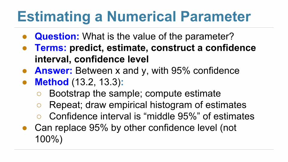
Estimating a Numerical Parameter● Question: What is the value of the parameter?● Terms: predict, estimate, construct a confidence

interval, confidence level● Answer: Between x and y, with 95% confidence● Method (13.2, 13.3):

○ Bootstrap the sample; compute estimate○ Repeat; draw empirical histogram of estimates○ Confidence interval is “middle 95%” of estimates

● Can replace 95% by other confidence level (not 100%)

Meaning of “95% Confidence”● You’ll never get to know whether or not your

constructed interval contains the parameter.

● The confidence is in the process that generates the interval.

● The process generates a good interval (one that contains the parameter) about 95% of the time.

● End of 13.2

Main Uses of Confidence Intervals● To estimate a numerical parameter: 13.3

○ Regression prediction, if regression model holds: Predict y based on a new x: 16.3

● To test whether or not a numerical parameter is equal to a specified value: 13.4○ In the regression model, used for testing whether the

slope of the true line is 0: 16.2

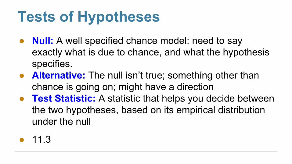
Tests of Hypotheses● Null: A well specified chance model: need to say

exactly what is due to chance, and what the hypothesis specifies.

● Alternative: The null isn’t true; something other than chance is going on; might have a direction

● Test Statistic: A statistic that helps you decide between the two hypotheses, based on its empirical distribution under the null

● 11.3

The P-value● The chance, under the null hypothesis, that the test

statistic comes out equal to the one in the sample or more in the direction of the alternative

● If this chance is small, then:○ If the null is true, something very unlikely has

happened.○ Conclude that the data support the alternative

hypothesis more than they support the null.● 11.3

An Error Probability● Even if the null is true, your random sample might

indicate the alternative, just by chance

● The cutoff for P is the chance that your test makes the wrong conclusion when the null hypothesis is true

● Using a small cutoff limits the probability of this kind of error

● Second half of 10.3, Lecture 18 (2/28) slides

Data in Two Categories● Null: The sample was drawn at random from a specified

distribution.● Test statistic: Either count/proportion in one category, or

distance between count/proportion and what you’d expect under the null; depends on alternative

● Method:○ Simulation: Generate samples from the distribution

specified in the null.● 11.1 (Swain v. Alabama, Mendel)

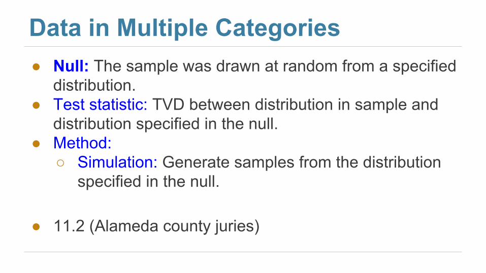
Data in Multiple Categories● Null: The sample was drawn at random from a specified

distribution.● Test statistic: TVD between distribution in sample and

distribution specified in the null.● Method:

○ Simulation: Generate samples from the distribution specified in the null.

● 11.2 (Alameda county juries)

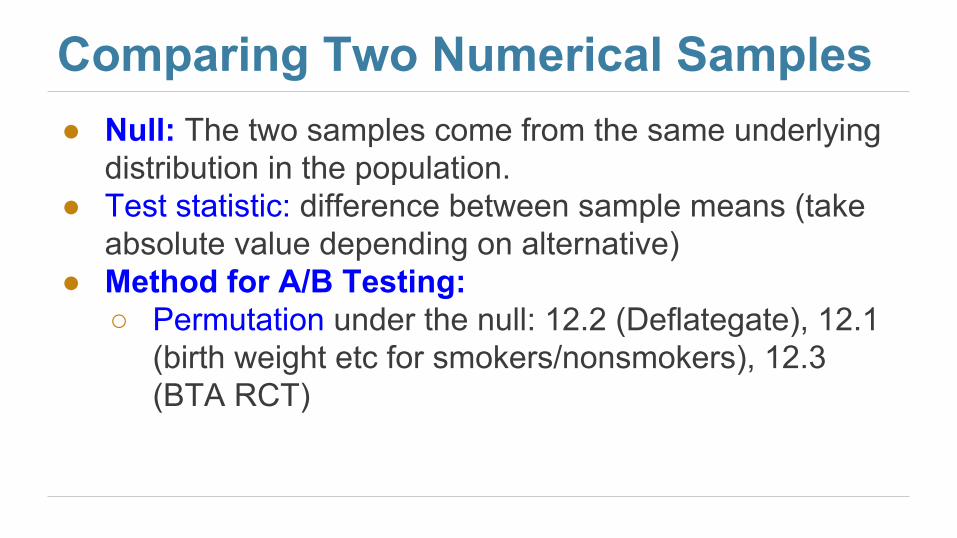
Comparing Two Numerical Samples● Null: The two samples come from the same underlying

distribution in the population.● Test statistic: difference between sample means (take

absolute value depending on alternative)● Method for A/B Testing:

○ Permutation under the null: 12.2 (Deflategate), 12.1 (birth weight etc for smokers/nonsmokers), 12.3 (BTA RCT)

One Numerical Parameter● Null: parameter = a specified value. ● Alternative: parameter ≠ value● Test Statistic: Statistic that estimates the parameter● Method:

○ Bootstrap: Construct a confidence interval and see if the specified value is in the interval.

● 13.4, 16.2 (slope of true line)

Causality● Tests of hypotheses can help decide that a difference is

not due to chance

● But they don’t say why there is a difference …

● Unless the data are from an RCT 12.3○ In that case a difference that’s not due to chance

can be ascribed to the treatment

Classification● Binary classification based on attributes 17.1

○ k-nearest neighbor classifiers● Training and test sets 17.2

○ Why these are needed○ How to generate them

● Implementation: 17.4○ Distance between two points○ Class of the majority of the k nearest neighbors

● Accuracy: Proportion of test set correctly classified 17.5