d. atdm experiments d-1. design of the task team experiment1 · d. atdm experiments d-1. design of...

73

D. ATDM experiments

D-1. Design of the Task Team Experiment1

The ATDMs used by the WMO Task Team members included MLDP0 (Modèle Lagrangien de

Dispersion de Particules d’ordre 0 – Canada; D’Amours et al., 2010), HYSPLIT (Hybrid Single-Particle Lagrangian Integrated Trajectory Model - United States; Draxler and Hess, 1997), NAME (Numerical Atmospheric-dispersion Modelling Environment - United Kingdom; Jones et al. 2007), RATM (Regional Atmospheric Transport Model – Japan; Shimbori et al., 2010), and FLEXPART (Lagrangian Particle Dispersion Model – Austria; Stohl et al., 2005). All ATDMs were of a class of models called Lagrangian Particle Dispersion Models (LPDMs). The transport and dispersion of individual pollutant particles or gases are simulated in a computational framework that follows the position of the individual element by its mean motion from the wind fields and a turbulent component to represent the dispersion. These models are all run in off-line mode, meaning that the meteorological fields needed as input to the ATDM have to be made available before the runs are conducted.

There were four global meteorological analyses data sets (Canada, United States, European Center for Medium-Range Weather Forecasts, UK Met Office) and two regional high-resolution analyses (Japan) available for use by the ATDMs. These data sets are briefly described in Table D-1-1.

Table D-1-1. Summary of the meteorological analyses fields available for the ATDM calculations.

Meteorological Center’s Product Acronym Space Time Vertical CMC’s Global Environmental Multiscale system

GEM 0.30o 6 h Sigma

NOAA’s Global Data Assimilation System GDAS 0.50o 3 h Hybrid sigma The European Centre for Medium-Range Weather Forecasts

ECMWF 0.125o and 0.2o

3 h Hybrid sigma

UKMET’s operational global Unified Model

MetUM 0.23o by 0.35o

3 h Height levels

JMA’s mesoscale analyses fields MESO 5 km 3 h Hybrid height levels

JMA’s radar-rain gauge-analyzed precipitation RAP 1 km 30 min Surface Each participating modeling center used its own dispersion model with one or more of the meteorological data sets, resulting in 18 different combinations of dispersion models and meteorological input data for the initial analysis provided to UNSCEAR (Table D-1-2) using their preliminary source term. Subsequently, JMA revised its dispersion model and two additional simulations were available for the task team summary (Draxler et al., 2015) that used the Terada (2012) source term.

1 R. Draxler

TECHNICAL REPORTS OF THE METEOROLOGICAL RESEARCH INSTITUTE No.76 2015

74

Table D-1-2. ATDM-Meteorology simulations completed (C) by each participating ATDM model

(rows) with different meteorological data (columns) and also the ATDM simulations enhanced with the RAP data (R).

Data / Model CMC NOAA ECMWF MetUM JMA CMC-MLDP0 C C JMA-RATM C,R NOAA-HYSPLIT C,R C,R C,R UKMET-NAME C C C,R ZAMG-FLEXPART

C,R C,R

One critical aspect for the quantitative predictions of air concentration and deposition is the wet

and dry scavenging that occurs along the particle’s transport pathway. Since following a large number of radionuclides could be computationally prohibitive, only three generic species were tracked as surrogates for all of the radionuclides: a gas with no wet or dry scavenging (noble gas), a gas with a relatively large dry deposition velocity and wet removal to represent gaseous 131I, and a particle with wet removal and a small dry deposition velocity to represent all the remaining radionuclide particles. There can be considerable variability in scavenging coefficients and deposition processes. Each ATDM had its own unique treatment of these processes which are described in more detail in Chapter F.

The ATDMs were all run “off-line” meaning that space and time varying meteorological data fields for the computational period must be available. The period of 11 – 31 March 2011 was determined to be the time window of greatest interest. Given the uncertainties in the emissions and the temporal frequency of meteorological analyses, the release periods were divided into three-hour duration segments. The emission rate is assumed to be a constant for each three-hour period. A separate 72 hour duration ATDM calculation was made for each radionuclide release period which was sufficiently long to permit particles to exit the regional sampling domain. After testing the ATDM calculations with several different particle number release rates and considering the regional nature and resolution of the concentration grid, the emissions were represented by the release of 100,000 particles per hour with a total mass of one unit per hour. Because of the uncertainty in the actual value of the time varying release height, particles were uniformly released from ground-level to 100 m.

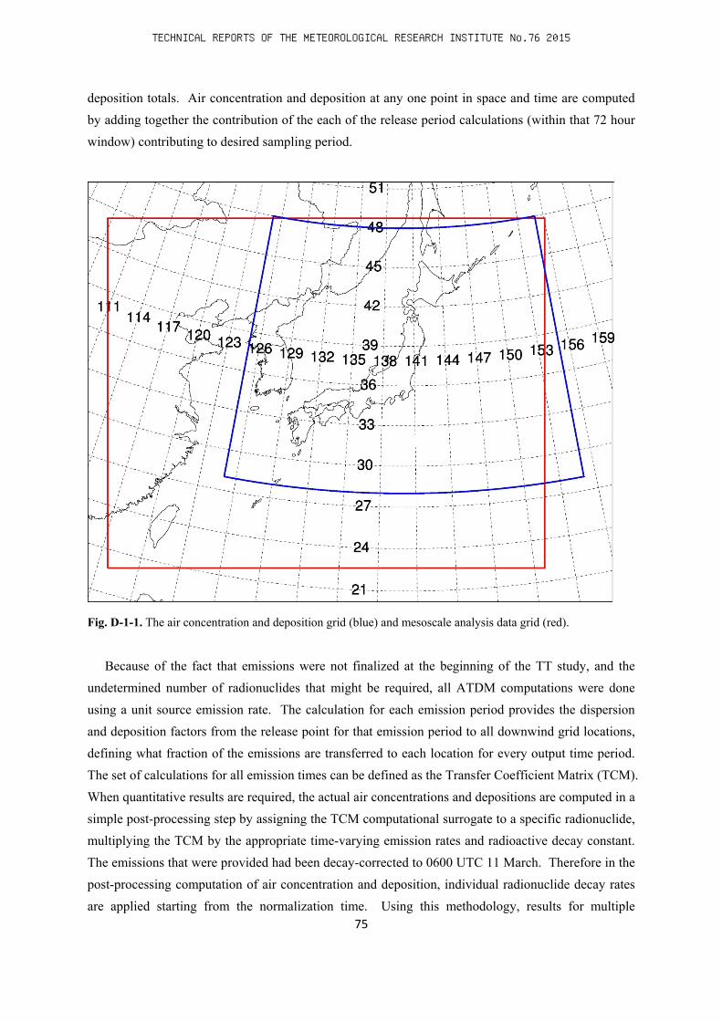
The ATDM calculations were started every three hours from 11 March 0000 UTC through 31 March 2100 UTC, resulting in 168 independent calculations. All ATDMs used a predefined concentration/deposition grid configuration of 601 (west to east) and 401 (south to north) grid cells on a regular latitude-longitude grid at 0.05 degrees resolution (about 5 km) centred at 38N and 140E (Fig. D-1-1). The output was configured to provide 3-hour averages for air concentrations and 3-hour


75

deposition totals. Air concentration and deposition at any one point in space and time are computed by adding together the contribution of the each of the release period calculations (within that 72 hour window) contributing to desired sampling period.

Fig. D-1-1. The air concentration and deposition grid (blue) and mesoscale analysis data grid (red).

Because of the fact that emissions were not finalized at the beginning of the TT study, and the

undetermined number of radionuclides that might be required, all ATDM computations were done using a unit source emission rate. The calculation for each emission period provides the dispersion and deposition factors from the release point for that emission period to all downwind grid locations, defining what fraction of the emissions are transferred to each location for every output time period. The set of calculations for all emission times can be defined as the Transfer Coefficient Matrix (TCM). When quantitative results are required, the actual air concentrations and depositions are computed in a simple post-processing step by assigning the TCM computational surrogate to a specific radionuclide, multiplying the TCM by the appropriate time-varying emission rates and radioactive decay constant. The emissions that were provided had been decay-corrected to 0600 UTC 11 March. Therefore in the post-processing computation of air concentration and deposition, individual radionuclide decay rates are applied starting from the normalization time. Using this methodology, results for multiple


76

emission scenarios can easily be obtained without rerunning any of the ATDMs. A detailed description of this approach is given by Draxler and Rolph (2012). The TCM concept is a specific operational realization of the source receptor matrix concept and similar to the backtracking computations to create Source Receptor Sensitivity Fields (Wotawa et. al., 2002).


D-2. Reverse estimation of amounts of 131I and 137Cs discharged into the atmosphere1 During the Fukushima Daiichi Nuclear Power Plant (FDNPP) accident, an urgent task was to assess

the radiological dose to the public resulting from the atmospheric release of radionuclides. This assessment was done by using both environmental monitoring data and computer simulations based on atmospheric dispersion modeling. However, source terms (e.g., the release rates and durations of radionuclides) essential to computer simulations of atmospheric dispersion were not available, although stack monitors or a severe accident analysis were expected to provide them. The Japan Atomic Energy Agency (JAEA), in cooperation with the Nuclear Safety Commission of Japan (NSC), has attempted to estimate the source terms of iodine and cesium discharged from FDNPP into the atmosphere by a reverse estimation method. In this method, the source terms are estimated by coupling environmental monitoring data with atmospheric dispersion simulations under the assumption of a unit release rate (1 Bq h–1). We estimated the release rates and total amounts of 131I and 137Cs discharged from FDNPP from 12 March to 1 May 2011.

D-2-1. Reverse estimation method The release rates of radionuclides (Bq h–1) are calculated by dividing measured atmospheric activity

concentrations of each radionuclide (131I and 137Cs) by simulated ones at each sampling point as follows:

iii CMQ = , (D-2-1)

where Qi is the release rate (Bq h–1) of radionuclide i into the atmosphere, Mi is the measured atmospheric activity concentration (Bq m–3) of radionuclide i, and Ci is the dilution factor (h m–3) of radionuclide i, which is equal to the activity concentration simulated under the assumption of a unit release rate (1 Bq h–1). Peak values from a time series of continuous measurement data were adopted

for both the measured and calculated values used in Eq. (D-2-1). If concentration data for the source term estimation were available from two or more different measurement sites at the same time, only the highest value was used in the release rate calculation.

When atmospheric activity concentration data were not available, the release rates were estimated by comparing measured air dose rates due to radionuclides in plumes and/or on the ground surface with simulated rates derived from the simulations with a unit release rate, by assuming the radionuclide composition (iodine, cesium, etc.).

Total release amounts were estimated by time integration of the release rates as follows:

[ ]∑ ×= jjii TQS , , (D-2-2)

where Si is the total released amount (Bq) of radionuclide i, Qi,j is the release rate (Bq h–1) of radionuclide i at time j, and Tj (h) is the duration of the period when the release rate Qi,j was estimated to continue. When no monitoring data were available at time j, release rates obtained before or after time j were temporally interpolated or extrapolated.

1 H. Terada and M. Chino

77


D-2-2. Environmental monitoring data Environmental monitoring data of atmospheric activity concentrations of iodine and cesium

(hereafter, dust sampling data) were mainly used for the source term estimation. We assumed that gaseous and particulate iodine were sampled according to the NSC’s guidelines for environmental radiation monitoring (NSC, 2010), which recommends the use of dust samplers with charcoal cartridges for gaseous iodine. The data used in the estimation are available on the web sites of the Ministry of Education, Culture, Sports, Science and Technology (MEXT) (MEXT, 2011a), the Ministry of Economy, Trade and Industry (METI) (METI, 2011), the Japan Chemical Analysis Center (JCAC) (JCAC, 2011), and JAEA (Furuta et al., 2011). These data were collected in eastern Japan, mainly Fukushima Prefecture. Air dose rate monitoring data from MEXT (MEXT, 2011b) and Fukushima Prefecture (Fukushima Prefecture, 2011a, 2011b) indicated that the atmospheric release of radionuclides in the daytime of 15 March resulted in a large amount of ground deposition and, thus, high dose rates in the sector to the northwest of FDNPP. However, because no dust monitoring data were available in the daytime of 15 March, the release rates of 131I and 137Cs at that time were estimated by comparing measured air dose rate patterns due to ground shine with simulated patterns after the plume had moved away from this region. Similarly, the release amount on the afternoon of 12 March was also estimated from ground shine. The measurement data used for source term estimation are described in detail by Chino et al. (2011), Katata et al. (2012a, 2012b), and Terada et al. (2012).

D-2-3. Atmospheric dispersion simulation The System for Prediction of Environmental Emergency Dose Information (SPEEDI) (MEXT,

2007), which is operated by the Nuclear Safety Technology Center of Japan, and the Worldwide version of SPEEDI (WSPEEDI-II) (Terada et al., 2008) developed by JAEA, were used for calculating atmospheric activity concentrations and air dose rates. The NSC provided the simulation results from SPEEDI to JAEA for the purpose of this source term estimation. Atmospheric dispersions of radionuclides were simulated by successive uses of the PHYSIC meteorological prediction model and the PRWDA21 atmospheric dispersion model in SPEEDI, and MM5 and GEARN in WSPEEDI-II. These models are described in detail by Nagai et al. (1999) and Terada and Chino (2008).

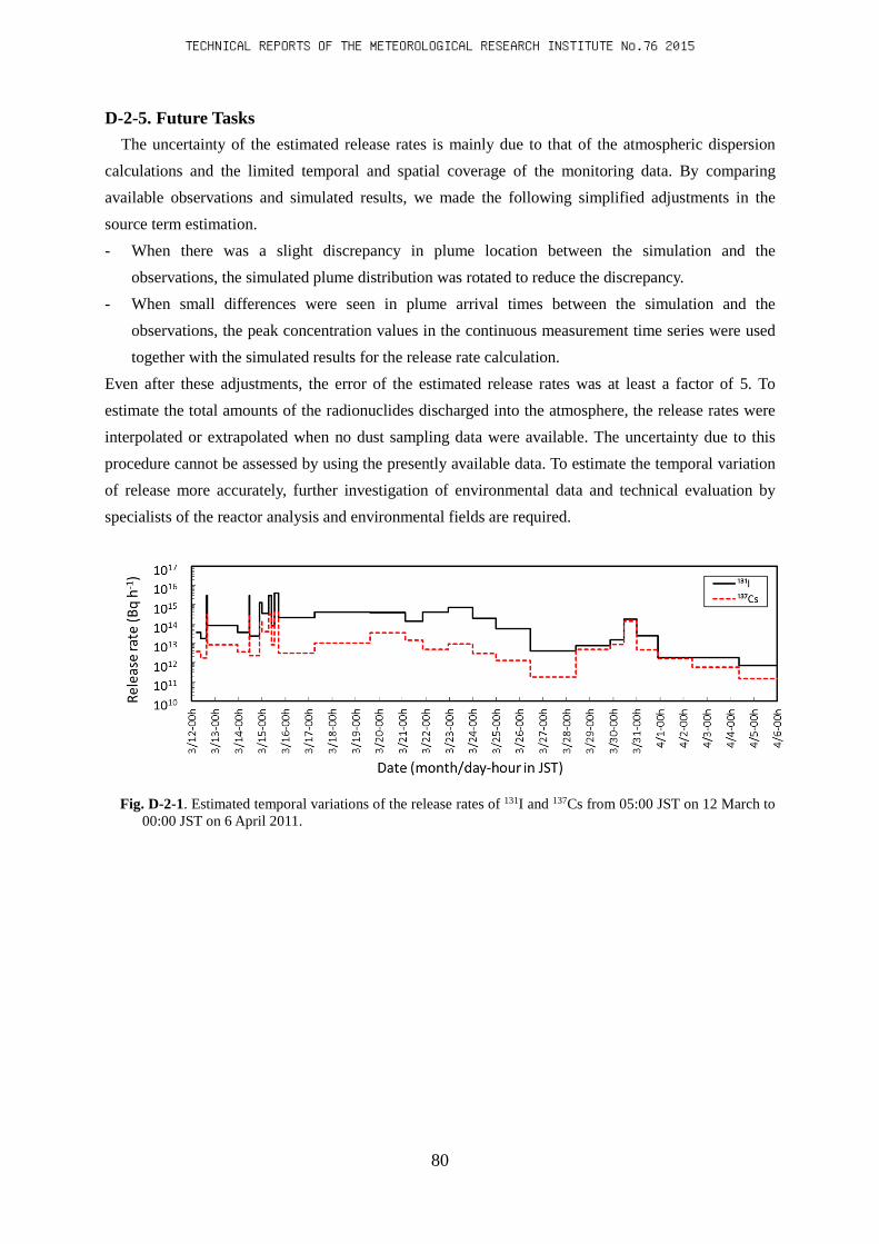
D-2-4. Results Figure D-2-1 shows the estimated temporal variation in release rates of 131I and 137Cs (Terada et al.,

2012) from 05:00 Japan Standard Time (JST = UTC + 9 h) on 12 March to 00:00 JST on 6 April 2011. Chino et al. (2011), Katata et al. (2012a, 2012b), and Terada et al. (2012) have described the source term estimation results in detail. Here, the estimation results are only outlined.

On the morning of 12 March, leakage of radionuclides from the Unit 1 primary containment vessel (PCV-U1) was detected, but the level of leakage was lower than that at later stages of the accident. At 15:36 JST on the afternoon of 12 March, a hydrogen explosion at Unit 1 increased the release rates of radionuclides. Between 15:30 and 16:00 JST, the estimated release rates were 3.0 × 1015 and 3.0 × 1014 Bq h–1 for 131I and 137Cs, respectively.

78


Venting operations were conducted to decrease the internal pressure of PCV-U3 at 09:24 and 12:30 JST on 13 March and at 05:20 JST on 14 March. However, the simulated plume mainly flowed toward the ocean on these days. In spite of these venting operations, a hydrogen explosion occurred at Unit 3 at 11:01 JST on 14 March. Because we had no sampling data from that time, we assumed that the release amounts were the same as those after the hydrogen explosion at Unit 1.

During the night of 14 March, dry venting was attempted at Unit 2. Though it is not clear whether the venting succeeded, the plume flowed south to south-southwest during this period. The observed air dose rates at Fukushima Daini Nuclear Power Plant (11.4 km to the south of FDNPP) and Kitaibaraki (80 km to the south) and atmospheric activity concentrations of 131I and 137Cs at JAEA-Tokai (100 km to the south) were high. By our source term estimation, the release rates of 3.5 × 1014 to 1.3 × 1015 Bq h–1 for 131I and of 4.0 × 1013 to 1.3 × 1014 Bq h–1 for 137Cs were estimated for the night of 14 March.

Between 07:00 and 12:00 JST on 15 March, the internal pressure of PCV-U2 decreased. This decrease corresponded to an extreme increase in the air dose rate to 1.5 × 104 µGy h–1, observed at the main gate from 07:00 to 10:00, which was clearly due to an increase in the release rate. The release rate from 07:00 to 10:00 was estimated to be 3.0 × 1015 for 131I and 3.0 × 1014 Bq h–1 for 137Cs. After

this major release on the morning of 15 March, the internal pressure of PCV-U2 continued to decrease during the afternoon. The plume discharged during the afternoon of 15 March was carried directly toward Iitate village and Fukushima City by southeasterly winds, and a large amount of wet deposition occurred northwest of FDNPP. From 13:00 to 17:00 JST on 15 March, the estimated release rates of 131I and 137Cs increased again, to 4.0 × 1015 and 4.0 × 1014 Bq h–1, respectively.

From 16 March to the early morning of 20 March, the plume was carried primarily toward the Pacific Ocean by westerly and northwesterly winds; consequently, too few monitoring data were available for estimating the source terms. Instead, we estimated the source terms during this period by temporal interpolation of those estimated during the period when observation data were available.

Beginning on 20 March, the direction of the plume again became landward. By this time, a systematic environmental monitoring had been established to measure atmospheric activity concentrations in Fukushima Prefecture. From 20 to 24 March, the estimated release rates of 131I and 137Cs were in the range of 1.4 × 1014 to 7.1 × 1014 Bq h–1 and 1.1 × 1012 to 3.5 × 1013 Bq h–1, respectively.

After 25 March, the estimated release rates gradually decreased, although a temporary increase to the rate on 20 March occurred on 30 March. Subsequently, the release rates decreased continuously, and from the beginning of April estimation of the source terms by the reverse estimation method was difficult because no clear increases in atmospheric activity concentrations and the air dose rates were detected.

Using Eq. (D2-2), we estimated the total amounts of 131I and 137Cs discharged into the atmosphere from 05:00 JST on 12 March to 00:00 JST on 1 May to be approximately 1.2 × 1017 and 8.8 × 1015 Bq, respectively.

79


D-2-5. Future Tasks The uncertainty of the estimated release rates is mainly due to that of the atmospheric dispersion

calculations and the limited temporal and spatial coverage of the monitoring data. By comparing available observations and simulated results, we made the following simplified adjustments in the source term estimation. - When there was a slight discrepancy in plume location between the simulation and the

observations, the simulated plume distribution was rotated to reduce the discrepancy. - When small differences were seen in plume arrival times between the simulation and the

observations, the peak concentration values in the continuous measurement time series were used together with the simulated results for the release rate calculation.

Even after these adjustments, the error of the estimated release rates was at least a factor of 5. To estimate the total amounts of the radionuclides discharged into the atmosphere, the release rates were interpolated or extrapolated when no dust sampling data were available. The uncertainty due to this procedure cannot be assessed by using the presently available data. To estimate the temporal variation of release more accurately, further investigation of environmental data and technical evaluation by specialists of the reactor analysis and environmental fields are required.

Fig. D-2-1. Estimated temporal variations of the release rates of 131I and 137Cs from 05:00 JST on 12 March to

00:00 JST on 6 April 2011.

80


81

D-3. Verification Methods1

The TT concluded that the most robust overall metric would be to evaluate the ATDM’s performance by comparing the model predicted patterns of 137Cs deposition to the available deposition measurements. The accumulated 137Cs deposition field has the advantage of the availability of measurements over a wide region. However, one disadvantage is that the bulk of the deposition occurred during only a few time periods. There are also no deposition measurements over water, effectively excluding all episodes with westerly winds from the analysis. In addition to deposition, there is considerable interest in how well the ATDM-meteorology combinations can represent the air concentration data. However, in terms of radionuclide specific measurements, air concentration data were available at only a few locations. Air dose rate measurements could not be used for the TT analysis.

To perform a quantitative analysis of the ATDM-meteorology combinations, the TT used the 137Cs deposition first reported by the Japanese Ministry of Education and Science and Technology (MEXT, 2011c). The ground-level results were merged with the observations by the U.S. Department of Energy’s (USDOE, 2011) fixed-wing aircraft (C-12) from 2 April 2011 to 9 May 2011. The collected aircraft and ground based data points were averaged onto a grid (0.05 degree resolution) that was identical to the one used in the ATDM calculations. The aircraft based sampling covered 374 grid points and blending in the additional ground based MEXT data resulted in a total of 543 grid points for model verification. Note that the final deposition product shown in Fig. D-3-1 captures the heaviest deposition in the Fukushima prefecture, but does not include any of the deposition to the southwest.

Fig. D-3-1. Averaged MEXT surface deposition and U.S. DOE aircraft based deposition measurements of 137Cs and the location of the Toki-Mura air sampling site.

1 R. Draxler


82

After the accident at the Fukushima Daiichi Nuclear Power Plant, radiation was monitored at the Nuclear Fuel Cycle Engineering Laboratories, Japan Atomic Energy Agency (JAEA) at their Tokai-Mura location (see Fig. D-3-1). Furuta et al. (2011) provides the monitoring results of dose rates, air concentrations, and deposition until 31 May 2011. The TT used the time series of 137Cs and 131I (aerosol and gas) air concentrations for the ATDM-meteorology evaluations for the 11-31 March period.

Procedures for evaluating ATDM calculations have a long history but the problem eludes simple solutions because the variability in atmospheric motions and processes cannot be deterministically represented in any model resulting in the inevitable mismatches between paired in space and time predicted and measured concentrations. The ATDM-meteorology evaluation protocol used here follows the procedure described by Draxler (2006), including a ranking method that gives equal weight to the normalized (0 to 1) sum of the correlation coefficient (R), the fractional bias (FB), the figure-of-merit in space (FMS), and the Kolmogorov-Smirnov parameter (KSP), such that the total model rank would range from 0 to 4 (from worst to best),

Rank = R2 + 1-|FB/2| + FMS/100 + (1-KSP/100). (D-3-1)

The correlation coefficient (R), also referred to as the Pearson’s Correlation Coefficient (PCC), is used to represent the scatter among paired measured (M) and predicted (P) values:

22

R)P(P)M(M

)P)(PM(M=

ii

ii , (D-3-2)

where the summation is taken over the number of samples and the over-bar represents a mean value. A normalized measure of bias is the fractional bias (FB). Positive values indicate over-prediction and FB ranges in value from –2 to +2 and it is defined by:

)M+P(

)MP(=

2FB . (D-3-3)

The normalized mean square error (NMSE) is defined as:

211NMSE ii PMNPM

= . (D-3-4)

The NMSE provides information on the deviations and not on the overestimation or underestimation. This parameter is very sensitive to differences between measured and predicted values. Perfect model results would have a NMSE value of zero. A similar metric is the root mean square error (RMSE), which is the square root of NMSE without normalization by (M-P).


83

The spatial distribution of the calculation relative to the measurements can be determined from the Figure of Merit in Space (FMS), which is defined as the percentage of overlap between measured and predicted areas. Rather than trying to contour sparse measurement data, the FMS is calculated as the intersection over the union of predicted (p) and measured (m) concentrations in terms of the number (N) of samplers with concentrations greater than a pre-defined threshold (zero):

MP

MP

NN

NN=

100FMS . (D-3-5)

Differences between the distribution of unpaired measured and predicted values is represented by the Kolmogorov-Smirnov parameter, which is defined as the maximum difference between two cumulative distributions when Mk = Pk, where

|)D(P)D(M|Max= kk KSP , (D-3-6)

and D is the cumulative distribution of the measured and predicted concentrations over the range of k values such that D is the probability that the concentration will not exceed Mk or Pk. It is a measure of how well the model reproduces the measured concentration distribution regardless of when or where it occurred. The maximum difference between any two distributions cannot be more than 100%.


84

D-4. The NOAA ARL Website1

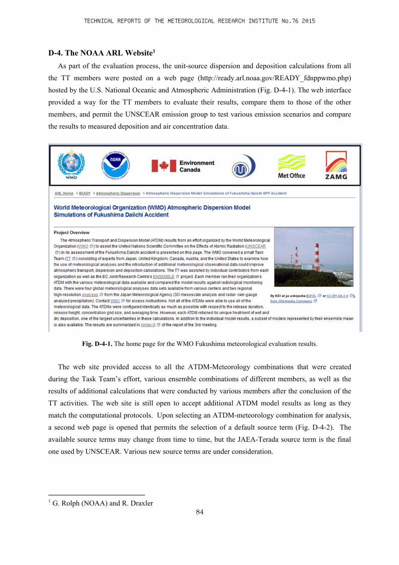
As part of the evaluation process, the unit-source dispersion and deposition calculations from all the TT members were posted on a web page (http://ready.arl.noaa.gov/READY_fdnppwmo.php) hosted by the U.S. National Oceanic and Atmospheric Administration (Fig. D-4-1). The web interface provided a way for the TT members to evaluate their results, compare them to those of the other members, and permit the UNSCEAR emission group to test various emission scenarios and compare the results to measured deposition and air concentration data.

Fig. D-4-1. The home page for the WMO Fukushima meteorological evaluation results.

The web site provided access to all the ATDM-Meteorology combinations that were created

during the Task Team’s effort, various ensemble combinations of different members, as well as the results of additional calculations that were conducted by various members after the conclusion of the TT activities. The web site is still open to accept additional ATDM model results as long as they match the computational protocols. Upon selecting an ATDM-meteorology combination for analysis, a second web page is opened that permits the selection of a default source term (Fig. D-4-2). The available source terms may change from time to time, but the JAEA-Terada source term is the final one used by UNSCEAR. Various new source terms are under consideration.

1 G. Rolph (NOAA) and R. Draxler


85

Fig. D-4-2. The source-term selection page.

Selection of any one source term just pre-populates the next page with 3-hourly values for 137Cs, and gaseous and particulate 131I (Fig. D-4-3). The web user may change the value of any of the pre-populated values to determine the effect on the final results. Although the source terms are defined for each 3-hour emission period, which corresponds to one ATDM simulation, the rate is given in Becquerels per hour. The emission entry page also permits the definition of any new species; the identification field is arbitrary, but the half-life and species type (noble gas, depositing gas, or particle) defines the subsequent calculation. The source term for each three-hour period is multiplied by the ATDM calculation for that time period and the air concentration and deposition grids from all ATDM simulations are added together for the same period to obtain the final values. Unless other species are requested to be included, the calculations will only be done for 137Cs. Each species requires another pass through all the data files.


86

Fig. D-4-3. Source term entry page.

Pressing the continue button opens the verification selection page (Fig. D-4-4) where the air concentration or deposition measurements used for verification may be selected. Only two air concentration locations with measurement data are available for selection (Tokai-Mura and Takasaki), although other locations can be entered to extract model predictions at those locations. The default deposition is the one used for the WMO Task Team effort, the combination of DOE airborne and MEXT ground based measurements. However, recently added were the results of the MEXT airborne survey of May 2012, which includes results from all the prefectures, not just Fukushima.


87

Fig. D-4-4. Verification selection page.

When the calculations have been completed, the model results page opens (not shown), which shows icons of the time series and scatter diagrams as well as text summaries of the statistical results. The deposition results have some text links rather than icons. Creating a deposition map requires a second step, where the time period as well as the contour intervals must be selected. Various output formats are available.


88

D-5. Task team final report and follow-up1 D-5-1. Task team final report and WMO technical publication

The final report of the Task Team was as uploaded as ANNEX III of the third meeting report on the website of WMO’s CBS-DPFS/ERA related Meetings page (http://www.wmo.int/pages/prog/www/CBS-Reports/documents/WMO_fnpp_final_AnnexIII_4Feb2013_REVISED_17June2013.pdf), and published as WMO technical publication No. 1120 (Draxler et al. 2013a). The UNSCEAR (Fischer 2012) and JMAEA source terms (Section D-2) were used for verification. In Section 10 of the above mentioned reports, an ensemble analysis and discussion on ATDM uncertainty based on UNSCEAR source term is included. In addition, a more complete discussion of the ensemble analyses has been published by Solazzo and Galmarini (2015).

D-5-2. Presentations at the 93rd meeting of AMS and EMS and related publications The 93rd American Meteorological Society annual meeting was held in Austin, Texas from January

6 to 10, 2013. A "Special Symposium on the Transport and Diffusion of Contaminants from the Fukushima Dai-Ichi Nuclear Power Plant: Present Status and Future Directions”; https://ams.confex.com/ams/93Annual/webprogram/FUKUSHIMASYMP.html) was organized there, and presentations were made on various topics such as an overview of the effects on the human body , emission source estimation, observations, limited model analysis, global ocean model analysis, and international cooperation. Draxler et al. (2013b) reported on the WMO Task Team results and Saito et al. (2013) presented JMA’s contribution to the WMO Task Team activities. The presentations of the symposium are summarized by Kondo et al., 2013. Wotawa et al. (2013) also reported on some of the task Team’s ATDM comparative experiments at the European Meteorological Society’s annual meeting.

Five papers relating to the Task Team activities have been published in the Fukushima nuclear accident special issue of the Journal of Environmental Radioactivity (Draxler et al., 2015; Arnold et al., 2015; Saito et al., 2015; Leadbetter et al., 2015; Solazzo and Galmarini, 2015).

D-5-3. UNSCEAR 60th General session and its final report The 60th General Assembly of UNSCEAR was held in Vienna from May 27 to 31, 2013

(http://www.unscear.org/unscear/en/about_us/sessions.html). The meeting report is available from the UNSCEAR website (http://daccess-ods.un.org/TMP/9420922.3985672.html). An UNSCEAR evaluation report on the Fukushima Daiichi nuclear power plant accident (UNSCEAR, 2014) was published separately in April 2014 as ANNEX A. From the task team final report, the results of the calculation of the NOAA ATDM and meteorological conditions were included in Appendix B.

1 K. Saito and R. Draxler


d. atdm experiments d-1. design of the task team experiment1 · d. atdm experiments d-1. design of...

Documents