MACFINROBODS – 612796 – FP7-SSH-2013-2

D10.6 – Quantitative or policy-oriented paper: The implications of introducing informational asymmetries and limitations in a model of optimal fiscal policy and debt

Project acronym: MACFINROBODS

Project full title: Integrated Macro-Financial Modelling for Robust Policy Design

Grant agreement no.: 612796

Due-Date: 31 March 2017 Delivery: 28 April 2017 Lead Beneficiary: CSIC Dissemination Level: PU Status: submitted Total number of pages: 41

This project has received funding from the European Union’s Seventh Framework Programme (FP7) for research, technological development and demonstration under grant agreement number 612796

On the Risk of Leaving the Euro and Maintaining

Austerity, the case of Greece∗

Manuel Macera† Albert Marcet‡ Juan Pablo Nicolini§

April 2017

Abstract

In the aftermath of the recent European sovereign debt crisis, there have been many

proposals to leave the Euro for South-European countries. Presumably, abandoning the

currency union would benefit these countries by allowing them to monetize deficits. In

this paper we argue that the risk of hyperinflation can be significant for these countries

if they leave the Euro with positive and persistent deficits, large value of debt to output

ratios. We consider a case when agents in the economy have incomplete information about

the economy, thus we depart from rational expectations. We use the recently developped

framework of ”internal rationality”. The paper also serves as a methodological exploration

of how to perform policy analysis under internal rationality.

∗The views expressed herein are those of the authors and do not necessarily those of the Federal Reserve Bankof Minneapolis or the Federal Reserve System. Marcet acknowledges partial support from SGR (Generalitat deCatalunya), from the European Research Council under the EU 7th Framework Programme (FP/2007-2013),Advanced Grant Agreement No. 324048, and the MACFINROBODS grant.†Colorado State University.‡ICREA, IAE, MOVE, and Universitat Autonoma de Barcelona.§Federal Reserve Bank of Minneapolis and Universidad Di Tella.

1. Introduction

We study a key policy decision using a model of imperfect information. The policy decision is

whether to leave the EMU while maintaining key fiscal policy variables unchanged and financing

debt with money creation. Imperfect information plays a role because we depart from rational

expectations. Instead we consider the case when consumers and investors do not understand

the consequences for inflation of such a change in policy but they form their expectations about

inflation by observing inflation after the event. We use the framework of ”internal rationality”,

where agents have limited information about how inflation behaves, but otherwise they behave

as rational agents.

Following the great world recession of 2008 and the European sovereign debt crisis of 2012,

the proposal to leave the Euro and reintroduce a national currency has regained support both

in academic and political circles. This proposal is gaining relevant support in some South-

European countries. Leaving the euro is supported in Italy by the Five Stars Movement and

Lega Norte, they got respectively 25% and 4% of the votes in the 2013 elections. In France,

Marine Le Pen, leader of the nationalist party Front National and the strongest supporter of

“Frexit”, is leading the last polls on April 2017 Presidential elections with 26% of consensus

(source: Odoxa and OpinionWay). In Greece, the radical-left party Syriza won the January

2015 elections with the promise to bargain favourable bailout conditions with Europe and, if

this was not possible, to leave the EMU.

As the story goes, leaving the euro would bring about many blessings: a reasonable amount

of inflation would help to lower government deficits, it would dilute huge levels of government

debt issued during the debt crisis and, therefore, paying unfair interest rates, currency deval-

uation would increase exports and output. Individual countries would be free from the fiscal

chains of the EU, putting an end to the fiscal austerity that is now eroding away the European

welfare state. One of the main reasons advocated by most Eurosceptic parties for leaving the

EU is substantially the recovery of national seignorage powers. In their view, re-launching

national currencies and allowing Central Banks to buy public debt printing fresh money would

leave governments free to adopt more expansionary measures to stimulate the economy, it would

bring in some healthy inflation, as opposed to the austerity required by some European rules

and the low inflation promoted by the ECB. Bernard Monot, Ms. Le Pen’s economic consultant

put it this way: “Give us the Banque de France and the Finance Ministry, then France would

be out of trouble in three weeks”. Alessandro di Battista from “Five Stars movement” said:

“We are convinced that, if we are able to take back monetary sovereignty we can raise Italy

from the rubble”.

The purpose of this paper is to evaluate the potential implications of leaving the euro

2

without increasing austerity.1 Furthermore, given the sovereign debt crisis that unravelled in

all these countries in 2010 and 2012, we assume they could not finance their deficits in bond

markets and they would have to resort to money financing of the deficit. We do not consider a

debt default; although this is obviously an alternative, it is a costly one.2

Then, the only flexibility that governments would indeed gain by leaving the euro is that

they would be free to monetize their government debt by issuing their newly recovered national

currencies.

We study this issue with a simple model of seignorage financing under three key assumptions.

First, we assume a deficit that is very persitent and exposed to volatile shocks. To consider the

case where austerity is not increased we assum that the process determining deficit will stay

the same after the exit. For this we use data for South-European countries to calibrate the

parameters for the deficit process, including its initial condition.

Our model is extremely simple and standard with one exception: we adopt the approach of

Internal Rationality, allowing for small departures from rational expectations while maintaining

full rationality of agents’ behavior.3 In our model agents have limited information about the

effects of such a policy change on inflation, therefore they learn how to forecast inflation by

observing inflation behavior itself. In this environment, agents’ expectations influence inflation

and inflation influences expectations. As shown by Marcet and Nicolini (2003), this departure

from rational expectations (RE) and this model explains key facts relating debt monetization,

inflation during the South-American hyperinflations of the 80’s, as well as the policies that were

put in place to stop those inflations. Therefore, this model is the starting point for the current

working paper.

The contribution of the paper is twofold. First, we show that the interaction of very per-

sistent deficits and severe difficulties to borrow in bond markets dramatically amplifies the

equilibrium inflation rates generated by the model under internal rationality. Thus, the paper

quantifies the risk of hyperinflations that may follow a departure of the Euro system for those

countries where this issue is now on the table. This risk seems to have been overlooked in the

recent debate.

Our second contribution is to start exploring the use internal rationality (IR) for policy

analysis. Departures from RE are still controversial in academic publications, specially when

they are used for policy analysis. After all, the main reason that RE became the dominant

1Some authors point out that inflation is desirable because it facilitates spending cuts by lowering real wagesof civil servants. But this only says that inflation is a useful trick to disguise austerity, civil servants’ purchasingpower would suffer anyway. Since we want to consider the case of not increasing austerity we effectively considerthe case that real wages of civil servants would not go down after leaving the euro.

2The costs of defaulting have been analyzed elsewhere and we do not study them here.3See Adam Marcet and Nicolini (2016) and Adam Marcet and Beutel (2017) for applications to stock market

volatility, and Adam and Marcet (2011) for a discussion of some theoretical issues.

3

paradigm is that it made it possible to analyze policy reforms in a consistent manner as it

addressed the Lucas critique. We claim that by explicitely modelling agents’ expectations we

can gain a better understanding of policy interventions.4

Under IR agents are assumed to hold beliefs about endogenous variables relevant to them

which are not the true distribution under the model considered. In the setup of this paper

agents will have a belief system about inflation. Unbeknownst to agents is the fact that given

these beliefs the model implies a certain mapping between aggregate shocks (in this case, shocks

to the government budget) and inflation. This raises three issues: i) is it logically consistent

to assume that agents are rational and that they ignore the model link between shocks and

inflation?, ii) what is a reasonable assumption about agents’ model for inflation, in other words,

if we depart from RE can we assume anything we want? and consequently obtain any possible

outcome of leaving the euro?, iii) how does a policy change expectations about inflation?. This

is how we deal with each of these issues:

i) we show how the assumption of RE is logically unrelated to the assumption of optimal

agents’ behavior. In a model with incomplete markets and heterogenous agents it is just

impossible for consumers to compute the RE equilibrium using only their (incomplete)

information about inflation behavior.5 Therefore agents are still saving and filtering

information optimally given their beliefs about inflation.

ii) we make an explicit assumption on the agents’ belief system about inflation, just like

many economics papers make assumptions about utility functions, production functions,

or equilibrium concept. Being explicit about this modelling choice (the agents’ system of

beliefs) has many advantages. First, it highlights the fact that, after all, RE is just one

assumption about agents’ beliefs from among many others. Second, it clarifies that this is

the only deviation from the standard paradigm that is now dominant in macroeconomics,

agents in our paper are completely rational given this system of beliefs.6 Third, we can

ask questions about how reasonable is this assumption vis a vis the data, observations on

agents’ expectations and the model itself.

As with any assumption, it is possible to justify our particular parametric choice by

discussing its modelling advantages and using empirical evidence. We think there are

4Obviously we are not the first to study policy analysis in models where agents have imperfect informationabout the model. What is new is the systematic use of IR in order to explore how expectations may behaveafter a policy change and to test these expectations in terms of the agents’ belief about the model.

5Adam and Marcet (2011) discuss a related issue in the context of stock markets.6The literature on adaptive learning as in, for example, Evans and Honkapohja (2002) and Marcet and

Sargent (1989a), was unclear about to which extent agents’ expectations were compatible with agents’ optimalbehavior, authors in that literature only claimed that agents were rational in the limit if the economy convergedto RE. IR clarifies this distinction: agents optimize given their system of beliefs about inflation, we make anexplicit assumption about this system, and this system is not equal to the behavior of inflation in the model.

4

the following advantages. First, the system of beliefs that we consider coincides with RE

beliefs for certain parameter values of the system of beliefs. In this way, we can study the

robustness of the predictions about leaving the Euro to small deviations from RE, and we

are precise about the meaning of this deviation. Second, we use empirical observations on

actual inflation and survey expectations to justify that people living in Southern-Europe

could possibly be endowed with this system of beliefs. Third, we imagine agents testing

their system of beliefs against model outcomes, if we find (as we check in the paper)

that their perceived model is hard to reject when inflation is generated by the model this

means that the system of beliefs could be sustained by the model. We call a system of

beliefs with all these properties ”a small deviation from RE”.

iii) The Lucas Critique argued that objects that were taken as given in old-style macro

models, such as the consumption function, were endogenous to policy, therefore those

models could not be used for policy analysis. Instead, the assumption of RE allowed

the researcher to model expectations in a way that is consistent with policy reform, the

savings function would most likely change because of the combination of a policy change

and RE so taking the savings function as given was logically inconsistent. We can level a

similar critique to RE: perhaps one may argue that in a stable system the economy may

be at a RE equilibrium, but if there is a large change in policy there is no reason why

agents’ beliefs about inflation may jump immediately to the new equilibrium. Therefore

the assumption of RE is endogenous to policy as well, and it is unlikely to be a reasonable

assumption precisely when there is a large change in policy. We think of the fact that

agents’ beliefs can be modelled in several ways (subject to the criteria of point ii) above)

as a healthy modelling method, as it forces the analyst to state his own uncertainty about

how agents’ expectations will react to a policy change, since in fact no economist is likely

to know for sure what will be the agents’ belief system after leaving the euro. We will

assume that agents maintain a belief system that represents explicitely uncertainty about

the underlying level of inflation, agents may re-set their prior about underlying inflation

after exiting, although we will focus on the case when agents’ beliefs stay stable after

leaving the euro, since this is the least favorable to the appearance of hyperinflations.

As we show, the implications of Leaving the Euro are not at all robust assuming RE. Under

RE an exit would only cause a mild inflation in many countries, so it may seem like a reasonable

alternative. But RE amounts to assuming agents’ inflation expectations are perfectly anchored

to the fundamentals of the economy.7 How could agents, in the midst of such a political

7Assuming Bayesian/RE models, where agents learn about fundamental processes as in scores of papersavailable in the literature (for example Andolfatto and Gomme (2004) in a monetary model) would have the

5

storm, know perfectly well the implications for inflation of exiting? If instead we assume

that agents have incomplete information, they may see inflation as driven by a permanent

and transitory component. Then agents would optimally learn about the best way to predict

the permanent component, and this gives expected inflation, therefore expected inflation is

likely to be influenced by observed inflation. High expected inflation discourages demand

for real balances in the national currency, thus inflation goes up, thus increasing expected

inflation firther and and so on. As in Marcet and Nicolini this can easily lead to hyperinflations.

According to our measures, the probability of hyperinflation would be very high when we

calibrate seignorage to the data of Greece.

Of course, if deficit was reduced after exiting the probability of a hyperinflation would go

down, but supposedly the reason for Leaving the Euro is precisely to avoid ”austerity”, so

Leaving the Euro is not a panacea against austerity.

To evaluate the adequacy of our assumption on the system of beliefs we perform a series of

tests (point ii) above) and show that for period lenghts of between 10 and 15 years, agents in

the model would not reject the hypothesis that their system of beliefs is the correct one. Thus,

given these sample sizes, there would not be enough evidence to contradict the beliefs agents

hold and, in this sense, this system of beliefs is a reasonable one for agents to maintain after

exiting. In a way, what happens is that just because agents believe that there is a permanent

component in the determination of inflation, then they learn about inflation and expected

inflation does become a permanent variable that influences true inflation. This is why they can

not reject their system of beliefs easily within the equilibrium inflation.

The paper proceeds as follows. In the next section we describe a heterogeneous agent model

with incomplete information showing that in our approach it is logically consistent to assume

agents that do not know the pricing function for inflation but that are fully rational. In Section

3 we introduce seignorage financing and study Learning Equilibria. In Section 4 we assess the

quantitative performance of our model and show that the presence of learning translates into

recurrent hyperinflationary episodes. In Section 5 we derive testable implications of the belief

system and test whether agents can reject their beliefs based on data generated by the model.

In Section 6 we conclude.

same problem: this literature assumes full knowledge of the pricing function, hence agents’ expectations areperfectly linked to fundamentals according to the model.

6

2. A Model with Heterogeneous Agents

Our basic model equation will be given by a government budget constraint and a money demand

equation where higher expected inflation drives down the demand for real balances as in (5).8

Here we take the simple approach, most commonly used in the literature, of deriving that

money demand from an overlapping generations model. However, it is also possible to derive

that equation from a model with long-lived agents and we will perform our derivations below

having this extension in mind. We consider heterogeneous agents to highlight the fact that

an individual agent would not be able to infer the pricing function from observations and her

own behavior, although the main analysis will be done with a homogeneous agent model for

simplicity. In addition to the money demand, the budget constraint of the government that

chooses to monetize debt will determine equilibrium.

Consider a constant cohort size, overlapping generations model in which each agent lives for

two periods. Agents are heterogeneous in their endowments and in their preferences, which are

determined by the moment they are born. The endowments of agent j ∈ [0, 1] born at time t

are normlized to 1 when young, and ej when old, and her preferences are given by

ln ct + αj lnxt+1

Thus agents are heterogeneous in their endowment when old ej and their discount factor αj.

We restrict the endowment when old to be smaller than the endowment when young (ej < 1

for all j). We assume that agents have a relative preference for consumption when old (αj > 1

for all j). These assumptions are made to ensure that as long as the return on savings is not

too low, young agents would save in equilibrium.

Markets are incomplete in the sense that the only asset agents can hold is fiat money. Thus,

at any point in time, there is only one spot market in which agents can exchange goods for

money, at a price Pt. When young, agents choose how many units of money to hold for next

period, given the price level that prevails at time t. The budget constraint when young is given

by9:

Ptcjt +M j

t ≤ Pt (1)

8Our model will be similar to Marcet and Nicolini (2003), we choose this setup as it has been shown toexplain well hyperinflationary episodes. The main difference in the present analysis will be considering variousalternatives for the fiscal deficit that reflect more closely deficit in European countries, so we will go away fromthe iid assumption for fiscal deficit.

9As agents cannot issue money, the constraint M jt ≥ 0 must be imposed. However, the assumption that the

endowment in the second period is smaller than in the first period implies this constraint will not be bindingas long as the inflation rate is not too high, thus we ignore this constraint in our theoretical analysis. In thenumerical section, we impose this constraint on the equilibrium.

7

In the following period, they consume their endowment plus whatever they can buy with the

money previously held, so their budget constraint when old is:

Pt+1xjt+1 ≤M j

t + ejPt+1 (2)

for all Pt+1.

Agents’ expectations are possibly heterogeneous as well, hence, the problem of agent of type

j born in period t consists in maximizing:

Ejt [ln ct + αj lnxt+1] (3)

by choosing consumption and money holdings, subject to the budget constraints (1) and (2).

Agents are assumed to observe at t the values of variables dated t as well as ej. However

agents do not know the value of next period prices level. Hence the expectation is taken with

respect to the price level Pt+1, which due to the presence of aggregate uncertainty agents can

not infer from their observed endowment, more on this later.

Since the budget constraints will hold with equality, once we substitute them in (3), an

interior solution requires:1

Pt −M jt

= Ejt

[αj

M jt + ejPt+1

](4)

which defines implicitly the individual money demand equation for agent j. Importantly, money

demand must be measurable with respect to the information set available when young. Since

the only source of uncertainty, namely Pt+1, appears in the denominator of the right hand side,

we cannot solve for the money demand equation in closed form. In order to make progress, we

study the linearized version of it, which can be written as10:

M jt

Pt= φj

(1− γjEj

t

Pt+1

Pt

)which corresponds to the money demand by each agent of generation t.

We have been working on various applications of internal rationality for a few years now.

In discussing our work, both in seminars and during the editorial process, we have found a

number of researchers in economics holding the view that a rational agent who knows the

process for exogenous fundamentals of an asset can not hold separately a view about the prices

of that asset. Such ”IR-skeptics” sustain that the whole structure of IR is logically inconsistent:

rational agents should be able to map their view of asset fundamentals into the value of an

10The linearization and the expressions for φjt and γjt are standard, they are offered for completeness in theAppendix.

8

asset price.

In the framework of this model we can formalize this view as follows: consider the assumption

Assumption 1 All agents hold a view about the evolution of the aggregate money supply M st .

An IR-skeptic would claim that under assumption 1 a rational agent should be able to infer

the pricing function that maps realizations of M s into a price level. The rest of the subsection

states that this argument is flawed for a variety of reasons. Therefore, we will conclude that IR

is logically consistent.

An IR-skeptic would likely articulate his thoughts using a homogeneous agent version of the

model. Notice that the above money demand with homogeneous agents is as follows

Mt = φ (Pt − γEtPt+1) (5)

Since knowledge of this equation is a consequence of rational behavior it must be that IR agents

know this equation. From this it follows that the price level (in a non-bubble solution) satisfies

Pt =1

φ

∞∑s=0

γsEtMst+s (6)

therefore knowledge of the aggregate money supply M s plus maximizing behavior by agents

indeed determines the price level and, according to an IR-skeptic it is then logically inconsistent

to assume (as we will assume below) that agents hold separate expectations about the price

level.

However, this argument does not work once we have heterogeneous agents. In this case the

only discounted sum one can obtain from knowledge of optimizing behavior is

Pt =1

φj

∞∑s=0

(γj)s

EjtM

jt+s (7)

The key difference is that the money demand in this expression is M j, with a super-index

corresponding to the agent j, not the exogenous supply for money as in (6). In other words,

the agent does know that his own optimal decision maps his future demands for money to the

price level, but optimal behavior does not relate future exogenous values of M s, hence there

is no contradiction in knowing the behavior of M s and having a separate belief system for the

price level, the first does not map into the second. The optimality condition (7) that agent j

knows to hold in a IR equilibrium in no way restricts what agents think about the link between

M s and P.

9

Since agents with different types will now face a different inference problem, the computation

of the right hand side of (7) becomes a much more complicated task. In particular, it requires

each agent knowing the inference problem solved by all other agents in the economy so that

agent i can figure out Ejt for all j 6= i. Even if we endow each agent with knowledge of the

distribution of types of all other agents in the economy, it is apparent that discovering the

mapping from exogenous variables to prices becomes a much more challenging problem.

But an IR-skeptic could bring to the table the following claim ”a rational agent could use

his rational behavior to infer the relationship aggregate money demand and, in this way, to

infer how M s and P are related”. Let’s see how this could work. Thus if we add some slight

knowledge about how other agents behave, individual optimization and knowledge of exogenous

variables maps into a price level.

Let us see how this could work. In the above model, aggregate money demand is:

Mt =

∫ 1

0

φj(Pt − γjEj

tPt+1

)dj. (8)

So, if in addition to knowing how to solve his maximization problem (ie, in addition to being

IR) we make the following assumption

Assumption 2 All agents know that other agents have similar utility function to their own,

up to diversity in γj, φj, Ej. Furthermore, agents know φ =∫ 1

0φjdj.

Under assumption 2 an IR agent could obtain

Pt =

∫ 1

0

φjγj

φEjtPt+1dj +

M st

φ. (9)

Is this enough to map M s into P?. The answer is no. All that our IR agent could do is to plug

the optimality condition (7) into (9) to obtain

Pt =

∫ 1

0

1

φEjt

∞∑s=0

(γj)s+1

M jt+1+sdj +

M st

φ(10)

so he needs to know, in addition,∫ 1

0Ejt (γj+1)

sM j

t+1+sdj for all t, s and these quantities can not

be inferred from the knowledge given under assumption 2.

Let us see under what assumptions the IR-skeptic would be right. Consider

Assumption 3 Agents have the same system of beliefs, therefore they have homogeneous (al-

though possibly non-RE) expectations Ej = EP .

10

Notice that under Assumptions 1 and 2 agents can figure out that

M jt = φj

(Pt − γjEPt Pt+1

)(11)

so that∫ 1

0

Ejt

(γj)s+1

M jt+1+sdj =

∫ 1

0

EPt(γj)s+1

φj(Pt+s+1 − γjPt+s+2

)dj

=

∫ 1

0

(γj)s+1

φj(EPt Pt+s+1 − γjEPt Pt+s+2

)dj

=

∫ 1

0

(γj)s+1

φjdj EPt Pt+s+1 −∫ 1

0

(γj)s+2

φjdj EPt Pt+s+2

for all j. But assumptions 1-3 still do not allow for the computation of this quantity, in addition

we would need to assume

Assumption 4 Agents know the whole joint distribution of γ, α

This assumption (but no less than this assumption) allows agents to compute the integrals∫ 1

0(γj)

s+1φjdj and

∫ 1

0(γj)

s+2φjdj in the last equation above. With this knowledge it is possible

indeed to map future values of M s into a price level today.

In other words, it is logically consistesn to assume that agents are rational and have price

beliefs that do not map M s into P as we do under Internal Rationality, all we need to assume

is agents do not know the distribution of other agents parameter utilities, and/or that their

beliefs are diverse.

Furthermore, in this paper we consider a model where the money supply is not exogenous,

but it is determined by the price level. Therefore, just because agents think inflation will

be different they will have different beliefs about the money supply. This means that even

assumption 1 is not reasonable in our model: in the event of a drastic policy change as the one

we consider in the paper, and if government deficits are going to be monetized, how could agents

know from the outset the behavior of money supply in the future given their price beliefs?.

3. Introducing Seignorage Financing

The model in the previous section highlighted the fact that representative agent models hide

valuable insight regarding how expectations must be formed. This implies that inflation expec-

tations may play a role in determining the model outcome even if agents are strictly rational

(by which we mean agents are internally rational, IR). We show that, indeed, the dynamics of

inflation expectations can play a crucial role in determining the outcome of a policy change.

11

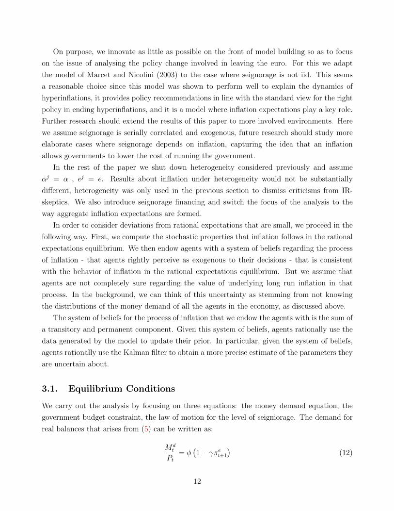
On purpose, we innovate as little as possible on the front of model building so as to focus

on the issue of analysing the policy change involved in leaving the euro. For this we adapt

the model of Marcet and Nicolini (2003) to the case where seignorage is not iid. This seems

a reasonable choice since this model was shown to perform well to explain the dynamics of

hyperinflations, it provides policy recommendations in line with the standard view for the right

policy in ending hyperinflations, and it is a model where inflation expectations play a key role.

Further research should extend the results of this paper to more involved environments. Here

we assume seignorage is serially correlated and exogenous, future research should study more

elaborate cases where seignorage depends on inflation, capturing the idea that an inflation

allows governments to lower the cost of running the government.

In the rest of the paper we shut down heterogeneity considered previously and assume

αj = α , ej = e. Results about inflation under heterogeneity would not be substantially

different, heterogeneity was only used in the previous section to dismiss criticisms from IR-

skeptics. We also introduce seignorage financing and switch the focus of the analysis to the

way aggregate inflation expectations are formed.

In order to consider deviations from rational expectations that are small, we proceed in the

following way. First, we compute the stochastic properties that inflation follows in the rational

expectations equilibrium. We then endow agents with a system of beliefs regarding the process

of inflation - that agents rightly perceive as exogenous to their decisions - that is consistent

with the behavior of inflation in the rational expectations equilibrium. But we assume that

agents are not completely sure regarding the value of underlying long run inflation in that

process. In the background, we can think of this uncertainty as stemming from not knowing

the distributions of the money demand of all the agents in the economy, as discussed above.

The system of beliefs for the process of inflation that we endow the agents with is the sum of

a transitory and permanent component. Given this system of beliefs, agents rationally use the

data generated by the model to update their prior. In particular, given the system of beliefs,

agents rationally use the Kalman filter to obtain a more precise estimate of the parameters they

are uncertain about.

3.1. Equilibrium Conditions

We carry out the analysis by focusing on three equations: the money demand equation, the

government budget constraint, the law of motion for the level of seigniorage. The demand for

real balances that arises from (5) can be written as:

Mdt

Pt= φ

(1− γπet+1

)(12)

12

where πet+1 = EPt[Pt+1

Pt

]denotes the expected gross inflation rate.

The only potential source of uncertainty in this model comes from the level of seigniorage.

In particular, the government budget constraint is given by:

M st = M s

t−1 + dtPt (13)

where M st is the money supply and dt denotes exogenous seigniorage, which evolves according

to:

dt = (1− ρ)δ + ρdt−1 + εt (14)

where εt denotes an i.i.d. perturbation term.

As mentioned in the introduction, this formulation is supposed to capture the feature that

upon abandoning a currency union, a country is unable to issue new net debt, it does not

default, it keeps primary deficit as before exiting, and must finance government deficit through

money printing11. Therefore dt is the real value of the secondary deficit of the government.

This generalizes Marcet and Nicolini (2003) in that it introduces serial correlation of seignor-

age, ρ 6= 0. We think this feature is important in studying a EMU exit as deficits are in fact

highly serially correlated and a proper calibration of this process is crucial for the results.

Expectations are taken using the subjective probability measure P . This probability mea-

sure specifies the joint distribution of {Pt}∞t=0 at all dates that agents hold and it is fixed at the

outset.

In equilibrium we must have Mdt = M s

t = Mt, which allows us to combine the money

demand equation (12) and the government budget constraint (13) to obtain:

πt =φ− φγπet

φ− φγπet+1 − dt(15)

where πt ≡ Pt/Pt−1 denotes the realized gross inflation rate. This equation governs the evolution

of inflation in any equilibrium, regardless of how expectations are formed, and we will use it

repeatedly.

We start by studying the rational expectations benchmark. Under rational expectations,

market prices are assumed to carry only redundant information because agents know the exact

mapping from the history of seigniorage levels to prices, Pt(dt). As usual we denote RE by

dropping the superscript P in the expectation operator and under RE we write:

πet+1 = Et[Pt+1

Pt

](16)

11In the quantitative section, we allow for policy regimes in which the government is able to deplete interna-tional reserves to finance its deficit.

13

3.2. The Rational Expectations Benchmark

We now study equilibria under RE, restricting attention first to a deterministic environment.

We focus on the case with persistence in the level of seignorage, which embeds the case studied

in ?.

In the absence of uncertainty, imposing rational expectations amounts to require πet = πt

for all t. Plugging this condition into the main equation (15) and rearranging delivers:

πt+1 = (1− ρ)

(φ+ φγ − δ

φγ− 1

γπt

)+ ρ

(φ+ φγ − dt−1

φγ− 1

γπt

)(17)

This equation will govern the dynamics of inflation in equilibrium.

The initial position of the economy is given by d0. Notice that if initial deficit is at the

mean d0 = δ, then under no uncertainty dt = δ for all t and the equilibrium will be stationary.

In such a case, (17) admits two stationary equilibria, which are obtained as the solutions to the

following quadratic equation:

φγπ2 − (φ+ φγ − δ)π + φ = 0 (18)

One could use this equation to trace out a stationary Laffer Curve, depicting the inflation rates

that allow the government to finance the level of seigniorage δ. We use {π1(δ),π2(δ)} to denote

the two roots of (18), where the small root π1(δ) corresponds to the ”good” side of the Laffer

Curve.

In the case in which d0 differs from δ then dt becomes a state variable of the model solution.

Now we define xt ≡ (πt, dt) and write the dynamic system composed of (14) and (17) as follows:

xt = G (xt−1) ≡

(1− ρ)F(πt−1, δ) + ρF(πt−1, dt−1) (1− ρ)δ + ρdt−1

(1− ρ)δ + ρdt−1

(19)

where

F(π, d) =φ+ φγ − d

φγ− 1

γπ(20)

In a deterministic environment, dt will always revert to its long run mean δ. Hence, to charac-

terize equilibria, it suffices to understand the behavior of πt, conditional on the initial position

d0. To this end, it will prove convenient to ensure that stationary inflation rates are always

positive and well-defined, for which we assume the following:

Assumption 5 δ ∈ D ≡ [0, φ(1 + γ − 2γ12 ))

14

One can easily check that under this assumption, stationary inflation rates are always within

the interval [1, γ−1]. Moreover, the upper bound of D can be interpreted as the maximum level of

seignorage that the government can finance, given the primitives of the economy. The following

proposition summarizes the behavior of inflation under Rational Expectations:

Proposition 1 Under Assumption 5, for any d0 ∈ D there exists π(d0) such that:

1. If π0 < π(d0), then limt→∞ πt = −∞

2. If π0 = π(d0), then limt→∞ πt = π1(δ)

3. If π0 > π(d0), then limt→∞ πt = π2(δ)

The proof is relegated to Appendix B. Notice that in the special case d0 = δ, one can show

that π(d0) = π1(δ) and the equilibrium is equivalent to that corresponding to the case with no

persistence.

The equilibria characterized in this proposition for the case d0 < δ is depicted in Figure ??.

The line with circles that starts at π(d0) represents the stable path that converges to the low

inflation steady state under Rational Expectations. For π0 6= π(d0), the lines with crosses show

the inflation paths that either converge to the high inflation steady state or diverge to infinity.

In the remainder of this section, we linearize (19) and introduce a small amount of uncer-

tainty in the seignorage to learn about the properties of the inflation process around the low

inflation steady state.

3.3. Inflation Persistence under Rational Expectations

To learn more about the stochastic properties of inflation in equilibrium, we linearize the main

equation (15) around the low inflation steady state and introduce a small amount of uncertainty

in the level of seigniorage. The linearization boils down to12:

πt =δ

φ− φγπ1(δ)− δdt (21)

=1

γπ2πt−1 −

δ

φγπdt (22)

dt = ρdt−1 + εt (23)

12See Appendix C for details.

15

where we are using the notation xt = lnxt − ln x, with bold letters indicating steady state

values. We can express inflation recursively as:

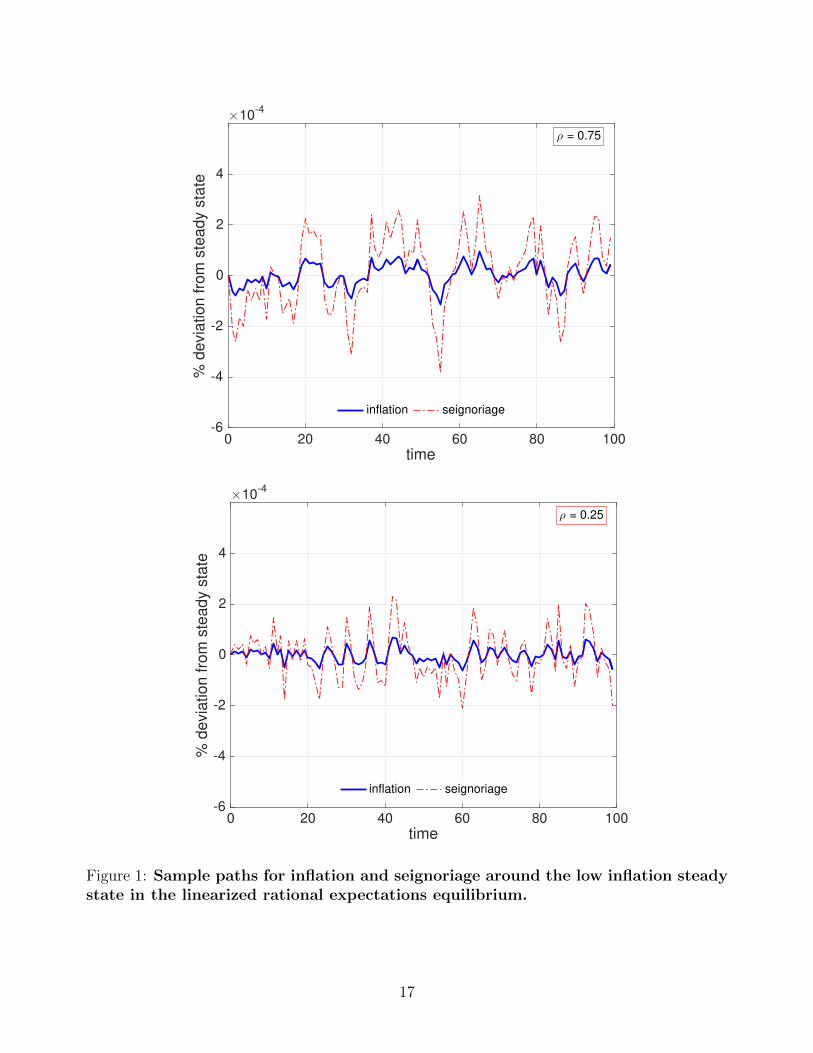
πt = ρπt−1 + νt (24)

where νt ≡ δεt/(φ−φγπ1(δ)−δ). Hence, around the low inflation steady state, inflation behaves

as an AR(1) process that inherits the persistence of seigniorage. Figure 1 displays sample paths

of both inflation and seigniorage according to this linearized system.

3.4. System of Beliefs about Inflation

We assume that agents hold the following beliefs regarding the inflation process:

πt = (1− ρπ) π?t + ρππt−1 + ut (25)

π?t = π?t−1 + ηt

where ut ∼ N(0, σ2u) and ηt ∼ N(0, σ2

η) are i.i.d. and independent of seignorage dt. We allow

for ρπ 6= ρ although in practice the difference will be small. The intuition behind the proposed

belief system (25) is that agents think inflation has a similar behavior as seignorage, so they

think it is an AR(1) process although they are unsure about the long run average level of

inflation π?t and they express their uncertainty about this long run level by modelling π?t as a

unit root process.

We choose this process for perceived inflation because it encompasses RE as a special case

when ρπ = ρ. In the IR equilibrium we assum agents take the serial correlation of inflation to

be close to that of seignorage, thus ρπ ' ρ.

Agents observe the realizations of inflation but not those of π?t and ut separately. Thus, the

learning problem consists of filtering long run inflation π?t out of observed inflation πt. Since

agents are rational their filter will involve using Bayes’ inference.

We denote the posterior mean of π?t entering period t given information available to agents

as βt = EP(π?t | πt−1). Agents are endowed with an initial prior belief about π?0 is normally

distributed with mean β0 = EP(π?0) and variance σ20 = EP(π?0 − β0)2. In most of the paper the

prior is assumed to be centered at the low inflation steady state β0 = π1(δ) with a variance

guranteeing that the gain in the Kalman filter is constant.

Notice that if we make σ2η = 0 then we assign probability 1 to β0 = π1(δ) so in this case:

πet = (1− ρπ)π1(δ) + ρππt−1 (26)

16

0 20 40 60 80 100time

-6

-4

-2

0

2

4

% d

evia

tio

n f

rom

ste

ad

y s

tate

×10-4

ρ = 0.75

inflation seignoriage

0 20 40 60 80 100time

-6

-4

-2

0

2

4

% d

evia

tio

n f

rom

ste

ad

y s

tate

×10-4

ρ = 0.25

inflation seignoriage

Figure 1: Sample paths for inflation and seignoriage around the low inflation steadystate in the linearized rational expectations equilibrium.

17

which, as long as ρπ = ρ, is equivalent to linearized RE equilibrium (24) for small deviations

around the low inflation steady state. In that sense, this setup encompasses rational expecta-

tions equilibria as a special case.

Under all these assumptions optimal learning then implies that βt evolves recursively ac-

cording to:

βt = βt +1

α

(πt − ρππt−1

1− ρπ− βt−1

)(27)

where α denotes the optimal Kalman gain13.

3.5. Learning Equilibria

The belief system implies that:

πet+1 = (1− ρπ)βt + ρππt (28)

Notice that if we plug this equation into (15) the solution is given by a non-linear equation

in πt so that multiple solutions may arise. To sidestep this problem, we assume that when

expectations regarding πet+1 are formed at period t, agents still do not know the realization

of πt. Therefore, in order to form their expectations regarding future inflation, they forecast

inflation two periods ahead using πt−1 as follows:

πet+1 =(1− ρ2π

)βt + ρ2ππt−1 (29)

Using this equation into (15) gives that equilibrium inflation follows

πt =φ− φγ((1− ρ2π) βt−1 + ρ2ππt−2)

φ− φγ((1− ρ2π) βt + ρ2ππt−1)− dt(30)

To provide intuition about the behavior of inflation in this case, let us write (30) as

H(βt, βt−1, πt, πt−1, πt−2, dt) = 0

and define h(β, π, d) ≡ H(β, β, π, π, π, d). The function h is useful to provide an approximation

of the behavior of inflation in a situation in which dt = δ, βt ≈ βt−1 and πt ≈ πt−1 ≈ πt−2 ≈βt−1. In such a case, (30) boils down to the quadratic equation (18), which implies that the

rational expectations stationary inflation rates are also stationary inflation rates under learning.

13In the quantitative section, and as is customary in models of learning, we will modify (27) to incorporateinformation regarding (πt − ρππt−1)/(1− ρπ) with a lag, in order to avoid the simultaneity between πt and βt.

18

However, notice that the stationary inflation rate πi(δ) is stable under learning only if:

∂π

∂β

∣∣∣β=πi(δ)

= −∂h/∂β∂h/∂π

∣∣∣β=πi(δ)

=φγπi(δ)− φγφ− φγπi(δ)− δ

< 1 (31)

As long as the denominator in (31) is positive14, we can verify that this is indeed the case if

and only if:

πi(δ) <φ+ φγ − δ

2φγ(32)

Using (18), it is easy to show that this condition is satisfied by the smallest root π1(δ), but not

by the largest π2(δ). Therefore, as pointed out in Marcet and Nicolini (2003) and Marcet and

Sargent (1989b), the low inflation Rational Expectations Equilibrium is stable under learning.

3.6. Justifying the System of Beliefs

As is clear from equation (30) in the learning equilibrium πt is a function of past seignorage.

However, agents think that inflation evolves according to the system of beliefs specified at the

beginning of section 3.4., which is obviously different from (30). This is not surprising to the

careful reader since, from the very beginning we have said that we depart from RE.

However, our aim is to consider only ”reasonable” systems of beliefs. Although IR permits

assuming anything you want for the system of beliefs, we do not think it is interesting to consider

systems of beliefs that generate inflation processes that render the beliefs to be ”obviously

wrong”. For this, we follow various principles that the belief system should satisfy

1. Encompass RE

In this way, there is a clear sense in which there is a small deviation from RE and that

the equilibrium does not deviate too much from the beliefs.

2. Close to the data

If the system of beliefs is close to the data behavior, and to the extent that the equilibrium

outcome of our model reproduces the behavior of data, we can expect that agents in the

real world can hold this system of beliefs and that this will in fact render the system close

to the model behavior.

3. Close to the model outcome

14Whenever there is a positive price that clears the money market, the denominator will be positive. Wecan always extend the model to include the case in which there are reserves that can be depleted to ensure theexistence of such a price, in the spirit of ?.

19

We would like to check that if agents observe the model outcome they can not reject their

belief system in a few periods. In this way we can think that the considered system of

beliefs is consistent with the model of inflation that we, as economists, consider.

4. Close to surveys

The system of beliefs should not be too different from observed surveys of expectations.

Since inflation surveys are conducted continuously in many countries it is possible to

apply this criterion to inflation.

The system of beliefs specified above turns out to satisfy all these criteria. 1- As explained

in section 3.4. the system of beliefs encompasses RE as a special case. 2- various authors

have chosen a similar model to explain actual inflation in various countries, for example Stock

and Watson (2007). Although they often use a more involved model including time varying

volatility, it often has the main features of our system of beliefs, namely serial correlation and

a permanent shock to average inflation. 3- We do a full array of tests to analyse how easy it

would be for agents to discover that their system of beliefs is not correct, we perform these

tests in section 5.. This implies that, given the system of beliefs, the equilibrium is such that

the agents see their belief system as a reasonable description of the inflation that they observe.

The reason that this is likely to happen has been described at the end of section

4- Many authors have fit the above model to inflation surveys, among others Roberts (1997).

4. Quantitative Performance

We analyse the behavior of the model under a calibration of the model parameters.

4.1. Calibration

Seignorage process and money demand

We assume that after exiting dt will follow a process similar to the secondary deficit before

exiting. This corresponds to a government that keeps austerity at similar levels as it was before

exiting, that does not default on the debt, and maintains a constant level of debt at the same

interest rate as before. Of course fiscal policy could differ after exiting, no one can know what

would actually happen, we could introduce different hypothesis for tax revenues, government

spending and debt issuance, find the implied evolution of d, and describe how inflation behaves

according to our model. Assuming the process for the secondary deficit will stay as before and

it will have to be financed by monetization seems to us a reasonable benchmark to consider.

20

The values of ρ and σε correspond to the estimation of an AR(1) process for Greece’s primary

balance as a percentage of GDP, so we focus on this country in the simulation exercise.

Money demand parameters target the inflation rate that maximizes the stationary Laffer

curve and the maximum seigniorage as a percentage of GDP for the case of Argentina, and

they are taken from Marcet and Nicolini.

Belief system

As explained in the introduction, the key methodological novelty in this paper is how to

perform policy analysis under IR. For this we have, first of all, shown that agents in our model

behave as rational agents even if they hold a belief system for inflation that is not equal to the

price equilibrium distribution of the model. Second, we have to specify the belief system for

agents after exiting. We simply proceed by stating clearly what are our assumptions about the

belief system after exiting. Of course, then there will be various assumptions one can make

about the belief system. This is unlike RE, where the belief system after the policy reform

is uniquely determined by the equilibrium. But we feel it is a good thing that we have to be

explicit about the various assumptions that one considers on the belief system after exiting

because, in fact, we do not know how expectations will be set after exiting. In this way,

economists are forced to express their ignorance about exactly how expectations will react to

such a policy change. By being explicit about our assumption on the system of beliefs we can

clarify the discussion about the likely outcome for inflation.

We keep the belief system specified in section 3.4.. This seems reasonable to us, agents

will not know what the new level of inflation will be. By assuming that the initial prior of

inflation β0 will be in the low inflation equilibrium we think we are conservatively estimating

the probability of a hyperinflation, after all these are countries where inflation was much higher

before the euro, although this recognises agents will understand that higher inflation than

under the euro is likely. Also, by assuming that σ0 delivers the steady state Kalman gain we

are stabilizing inflation and, therefore, delaying hyperinflations: an alternative would be to

consider that there is very high initial uncertainty so σ0 is initially quite high.

We set ρπ = ρ, which is a reasonable assumption as we show in the appendix.

Policy Rules with ERR

We now introduce policy rules that modify, in some periods, the determination of inflation.

The reason for these rules is two-fold: first, similar rules have been used in countries that

experienced very high or very low inflations, second, they insure existence of equilibrium in

the learning model, as there may be no positive price level that clears the market for arbitrary

expectations.

In any event, the particular assumption we make on this front is inconsequential for the

21

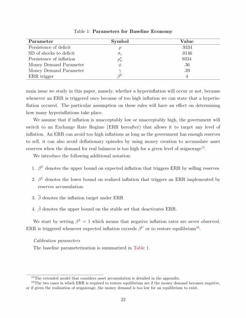
Table 1: Parameters for Baseline Economy

Parameter Symbol ValuePersistence of deficit ρ .9334SD of shocks to deficit σε .0146Persistence of inflation ρ?π 9334Money Demand Parameter φ .36Money Demand Parameter γ .39ERR trigger βU 4

main issue we study in this paper, namely, whether a hyperinflation will occur or not, because

whenever an ERR is triggered once because of too high inflation we can state that a hyperin-

flation occured. The particular assumption on these rules will have an effect on determining

how many hyperinflations take place.

We assume that if inflation is unacceptably low or unacceptably high, the government will

switch to an Exchange Rate Regime (ERR hereafter) that allows it to target any level of

inflation. An ERR can avoid too high inflations as long as the government has enough reserves

to sell, it can also avoid deflationary episodes by using money creation to accumulate asset

reserves when the demand for real balances is too high for a given level of seignorage15.

We introduce the following additional notation:

1. βU denotes the upper bound on expected inflation that triggers ERR by selling reserves

2. βL denotes the lower bound on realized inflation that triggers an ERR implemented by

reserves accumulation.

3. β denotes the inflation target under ERR

4. β denotes the upper bound on the stable set that deactivates ERR.

We start by setting βL = 1 which means that negative inflation rates are never observed.

ERR is triggered whenever expected inflation exceeds βU or to restore equilibrium16.

Calibration parameters

The baseline parameterization is summarized in Table 1.

15The extended model that considers asset accumulation is detailed in the appendix.16The two cases in which ERR is required to restore equilibrium are if the money demand becomes negative,

or if given the realization of seigniorage, the money demand is too low for an equilibrium to exist.

22

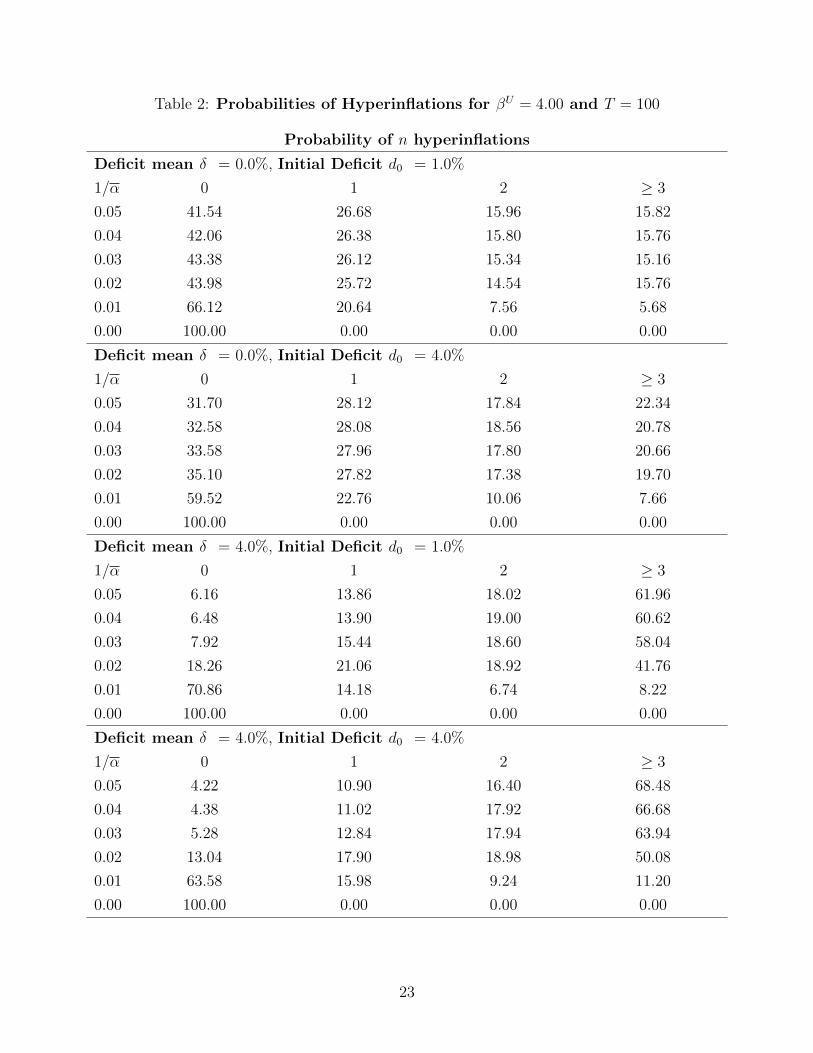
Table 2: Probabilities of Hyperinflations for βU = 4.00 and T = 100

Probability of n hyperinflations

Deficit mean δ = 0.0%, Initial Deficit d0 = 1.0%

1/α 0 1 2 ≥ 3

0.05 41.54 26.68 15.96 15.82

0.04 42.06 26.38 15.80 15.76

0.03 43.38 26.12 15.34 15.16

0.02 43.98 25.72 14.54 15.76

0.01 66.12 20.64 7.56 5.68

0.00 100.00 0.00 0.00 0.00

Deficit mean δ = 0.0%, Initial Deficit d0 = 4.0%

1/α 0 1 2 ≥ 3

0.05 31.70 28.12 17.84 22.34

0.04 32.58 28.08 18.56 20.78

0.03 33.58 27.96 17.80 20.66

0.02 35.10 27.82 17.38 19.70

0.01 59.52 22.76 10.06 7.66

0.00 100.00 0.00 0.00 0.00

Deficit mean δ = 4.0%, Initial Deficit d0 = 1.0%

1/α 0 1 2 ≥ 3

0.05 6.16 13.86 18.02 61.96

0.04 6.48 13.90 19.00 60.62

0.03 7.92 15.44 18.60 58.04

0.02 18.26 21.06 18.92 41.76

0.01 70.86 14.18 6.74 8.22

0.00 100.00 0.00 0.00 0.00

Deficit mean δ = 4.0%, Initial Deficit d0 = 4.0%

1/α 0 1 2 ≥ 3

0.05 4.22 10.90 16.40 68.48

0.04 4.38 11.02 17.92 66.68

0.03 5.28 12.84 17.94 63.94

0.02 13.04 17.90 18.98 50.08

0.01 63.58 15.98 9.24 11.20

0.00 100.00 0.00 0.00 0.00

23

0 20 40 60 80 1000

1

2

3

4

5

6

7 8 9 10

quart

erly inflation r

ate

(lo

g s

cale

)

1/α = 0.051/α = 0.00

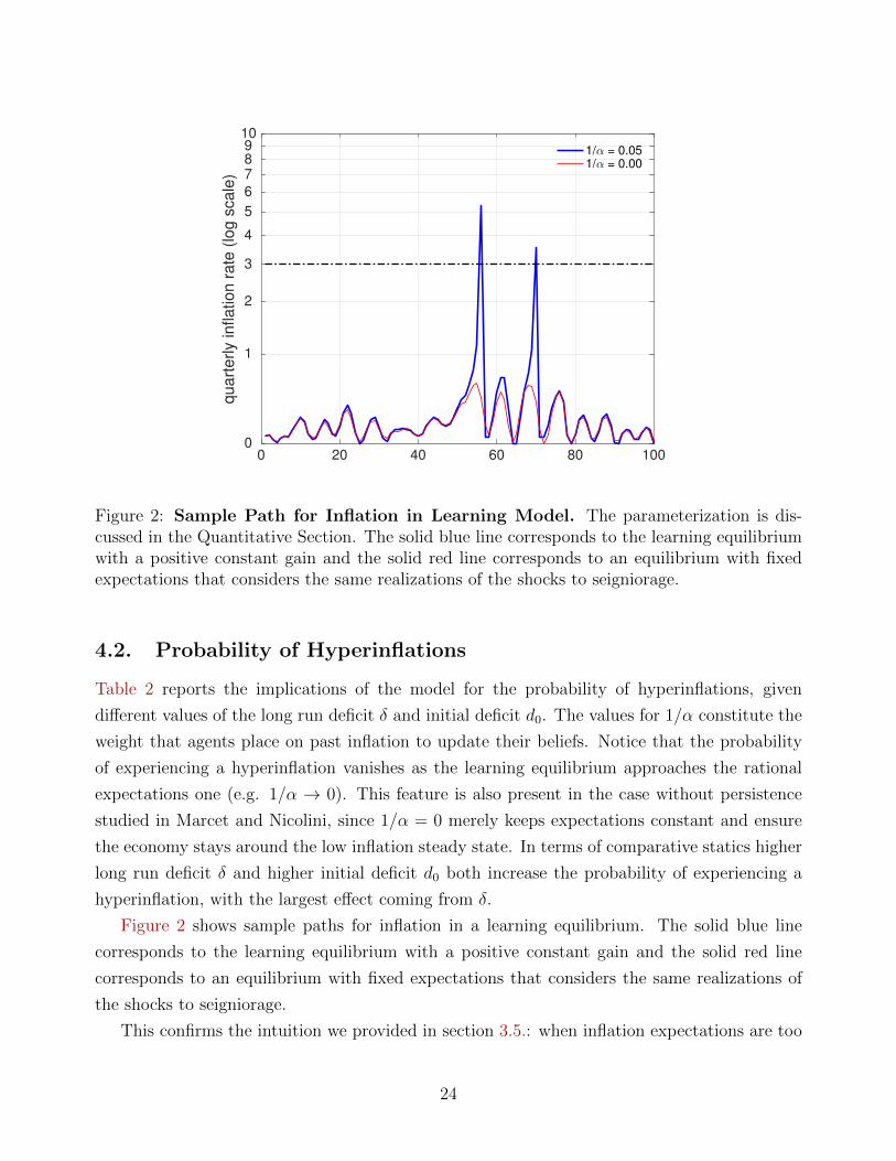
Figure 2: Sample Path for Inflation in Learning Model. The parameterization is dis-cussed in the Quantitative Section. The solid blue line corresponds to the learning equilibriumwith a positive constant gain and the solid red line corresponds to an equilibrium with fixedexpectations that considers the same realizations of the shocks to seigniorage.

4.2. Probability of Hyperinflations

Table 2 reports the implications of the model for the probability of hyperinflations, given

different values of the long run deficit δ and initial deficit d0. The values for 1/α constitute the

weight that agents place on past inflation to update their beliefs. Notice that the probability

of experiencing a hyperinflation vanishes as the learning equilibrium approaches the rational

expectations one (e.g. 1/α → 0). This feature is also present in the case without persistence

studied in Marcet and Nicolini, since 1/α = 0 merely keeps expectations constant and ensure

the economy stays around the low inflation steady state. In terms of comparative statics higher

long run deficit δ and higher initial deficit d0 both increase the probability of experiencing a

hyperinflation, with the largest effect coming from δ.

Figure 2 shows sample paths for inflation in a learning equilibrium. The solid blue line

corresponds to the learning equilibrium with a positive constant gain and the solid red line

corresponds to an equilibrium with fixed expectations that considers the same realizations of

the shocks to seigniorage.

This confirms the intuition we provided in section 3.5.: when inflation expectations are too

24

large it is likely that hyperinflationary paths start to appear, these are then stopped by ERR

rules, but if average seignorage is too high these hyperinflations are activated again.

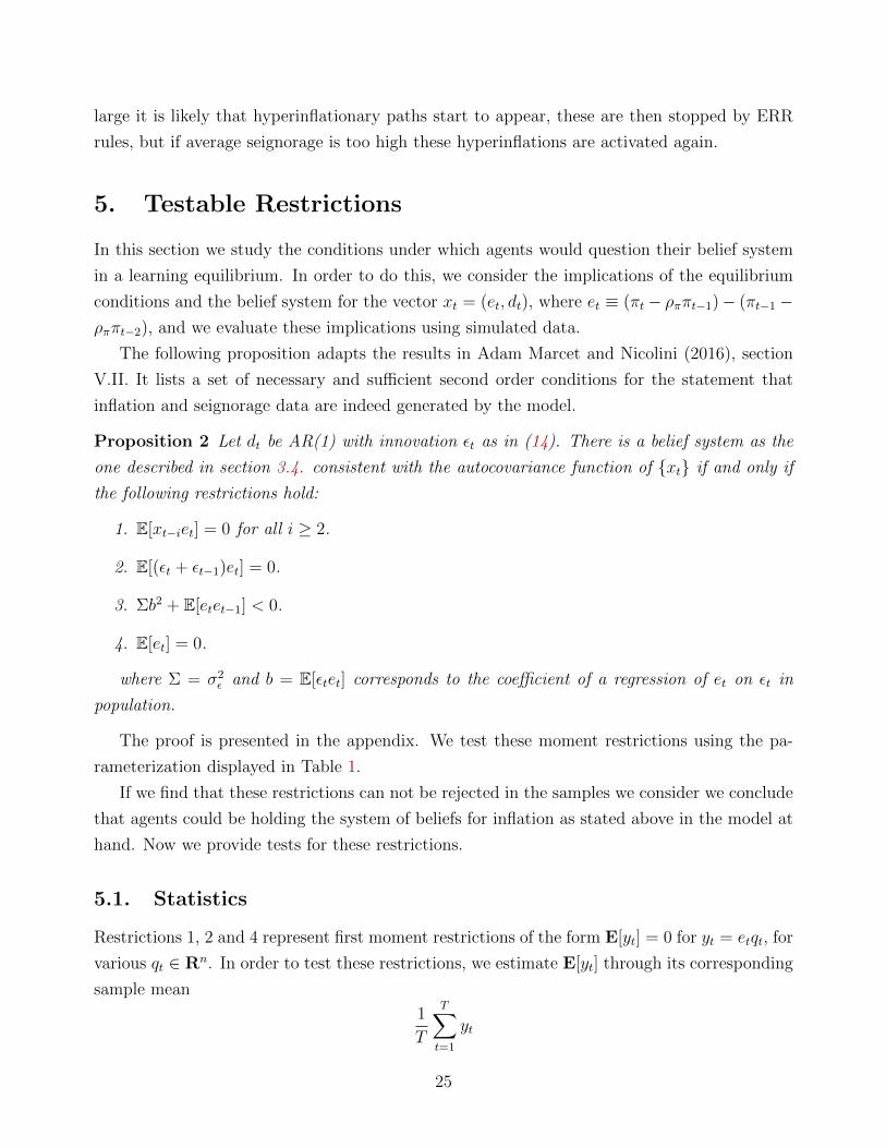
5. Testable Restrictions

In this section we study the conditions under which agents would question their belief system

in a learning equilibrium. In order to do this, we consider the implications of the equilibrium

conditions and the belief system for the vector xt = (et, dt), where et ≡ (πt − ρππt−1)− (πt−1 −ρππt−2), and we evaluate these implications using simulated data.

The following proposition adapts the results in Adam Marcet and Nicolini (2016), section

V.II. It lists a set of necessary and sufficient second order conditions for the statement that

inflation and seignorage data are indeed generated by the model.

Proposition 2 Let dt be AR(1) with innovation εt as in (14). There is a belief system as the

one described in section 3.4. consistent with the autocovariance function of {xt} if and only if

the following restrictions hold:

1. E[xt−iet] = 0 for all i ≥ 2.

2. E[(εt + εt−1)et] = 0.

3. Σb2 + E[etet−1] < 0.

4. E[et] = 0.

where Σ = σ2ε and b = E[εtet] corresponds to the coefficient of a regression of et on εt in

population.

The proof is presented in the appendix. We test these moment restrictions using the pa-

rameterization displayed in Table 1.

If we find that these restrictions can not be rejected in the samples we consider we conclude

that agents could be holding the system of beliefs for inflation as stated above in the model at

hand. Now we provide tests for these restrictions.

5.1. Statistics

Restrictions 1, 2 and 4 represent first moment restrictions of the form E[yt] = 0 for yt = etqt, for

various qt ∈ Rn. In order to test these restrictions, we estimate E[yt] through its corresponding

sample mean

1

T

T∑t=1

yt

25

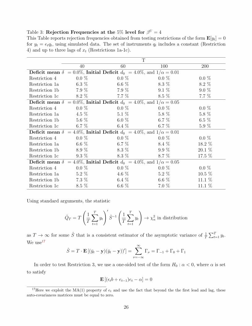
Table 3: Rejection Frequencies at the 5% level for βU = 4This Table reports rejection frequencies obtained from testing restrictions of the form E[yt] = 0for yt = etqt, using simulated data. The set of instruments qt includes a constant (Restriction4) and up to three lags of xt (Restrictions 1a-1c).

T40 60 100 200

Deficit mean δ = 0.0%, Initial Deficit d0 = 4.0%, and 1/α = 0.01Restriction 4 0.0 % 0.0 % 0.0 % 0.0 %Restriction 1a 6.3 % 6.6 % 8.3 % 8.2 %Restriction 1b 7.9 % 7.9 % 9.1 % 9.0 %Restriction 1c 8.2 % 7.7 % 8.5 % 7.7 %Deficit mean δ = 0.0%, Initial Deficit d0 = 4.0%, and 1/α = 0.05Restriction 4 0.0 % 0.0 % 0.0 % 0.0 %Restriction 1a 4.5 % 5.1 % 5.8 % 5.8 %Restriction 1b 5.6 % 6.0 % 6.7 % 6.5 %Restriction 1c 6.7 % 6.4 % 6.7 % 5.9 %Deficit mean δ = 4.0%, Initial Deficit d0 = 4.0%, and 1/α = 0.01Restriction 4 0.0 % 0.0 % 0.0 % 0.0 %Restriction 1a 6.6 % 6.7 % 8.4 % 18.2 %Restriction 1b 8.9 % 8.3 % 9.9 % 20.1 %Restriction 1c 9.3 % 8.3 % 8.7 % 17.5 %Deficit mean δ = 4.0%, Initial Deficit d0 = 4.0%, and 1/α = 0.05Restriction 4 0.0 % 0.0 % 0.0 % 0.0 %Restriction 1a 5.2 % 4.6 % 5.2 % 10.5 %Restriction 1b 7.3 % 6.4 % 6.6 % 11.1 %Restriction 1c 8.5 % 6.6 % 7.0 % 11.1 %

Using standard arguments, the statistic

QT = T

(1

T

T∑t=1

yt

)′S−1

(1

T

T∑t=1

yt

)→ χ2

n in distribution

as T → ∞ for some S that is a consistent estimator of the asymptotic variance of 1T

∑Tt=1 yt.

We use17

S = T · E [(yt − y)(yt − y))′] =∞∑

ν=−∞

Γν = Γ−1 + Γ0 + Γ1

In order to test Restriction 3, we use a one-sided test of the form H0 : α < 0, where α is set

to satisfy

E [(εtb+ et−1)et − α] = 0

17Here we exploit the MA(1) property of et and use the fact that beyond the the first lead and lag, theseauto-covariances matrices must be equal to zero.

26

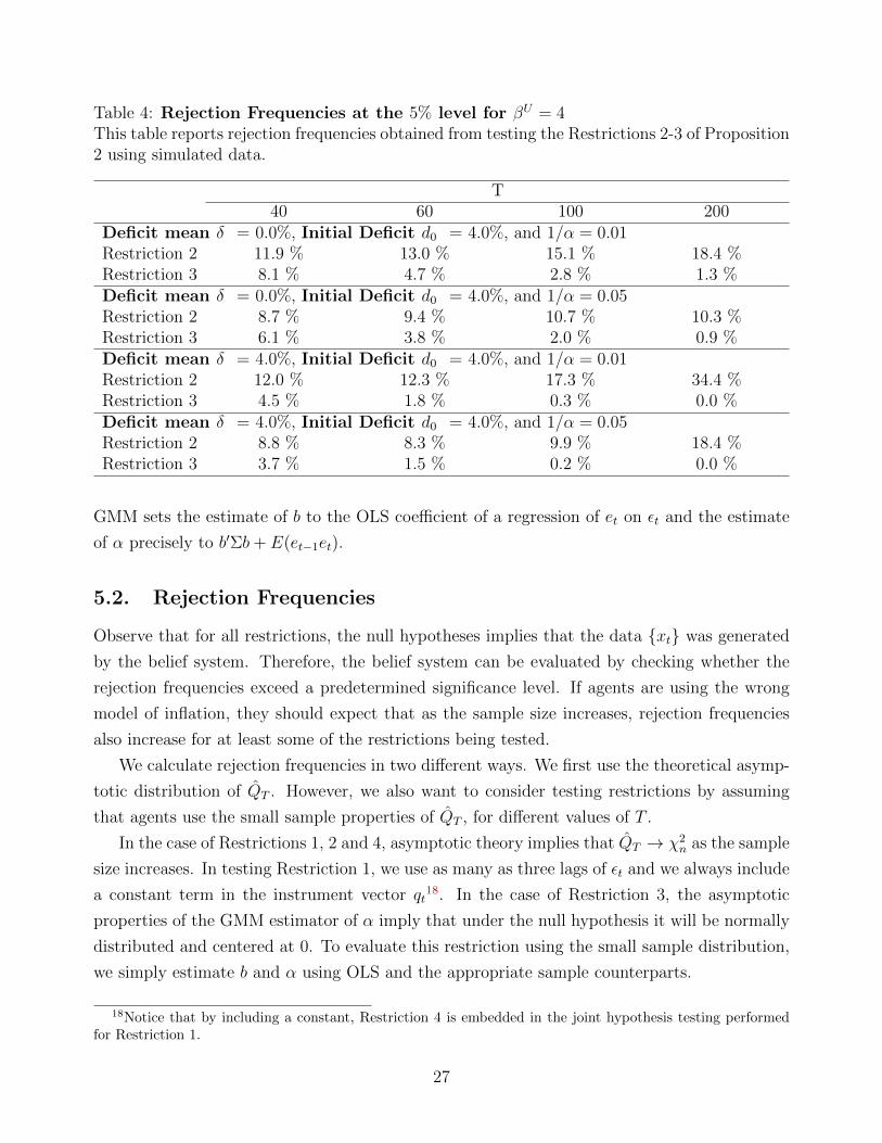
Table 4: Rejection Frequencies at the 5% level for βU = 4This table reports rejection frequencies obtained from testing the Restrictions 2-3 of Proposition2 using simulated data.

T40 60 100 200

Deficit mean δ = 0.0%, Initial Deficit d0 = 4.0%, and 1/α = 0.01Restriction 2 11.9 % 13.0 % 15.1 % 18.4 %Restriction 3 8.1 % 4.7 % 2.8 % 1.3 %Deficit mean δ = 0.0%, Initial Deficit d0 = 4.0%, and 1/α = 0.05Restriction 2 8.7 % 9.4 % 10.7 % 10.3 %Restriction 3 6.1 % 3.8 % 2.0 % 0.9 %Deficit mean δ = 4.0%, Initial Deficit d0 = 4.0%, and 1/α = 0.01Restriction 2 12.0 % 12.3 % 17.3 % 34.4 %Restriction 3 4.5 % 1.8 % 0.3 % 0.0 %Deficit mean δ = 4.0%, Initial Deficit d0 = 4.0%, and 1/α = 0.05Restriction 2 8.8 % 8.3 % 9.9 % 18.4 %Restriction 3 3.7 % 1.5 % 0.2 % 0.0 %

GMM sets the estimate of b to the OLS coefficient of a regression of et on εt and the estimate

of α precisely to b′Σb+ E(et−1et).

5.2. Rejection Frequencies

Observe that for all restrictions, the null hypotheses implies that the data {xt} was generated

by the belief system. Therefore, the belief system can be evaluated by checking whether the

rejection frequencies exceed a predetermined significance level. If agents are using the wrong

model of inflation, they should expect that as the sample size increases, rejection frequencies

also increase for at least some of the restrictions being tested.

We calculate rejection frequencies in two different ways. We first use the theoretical asymp-

totic distribution of QT . However, we also want to consider testing restrictions by assuming

that agents use the small sample properties of QT , for different values of T .

In the case of Restrictions 1, 2 and 4, asymptotic theory implies that QT → χ2n as the sample

size increases. In testing Restriction 1, we use as many as three lags of εt and we always include

a constant term in the instrument vector qt18. In the case of Restriction 3, the asymptotic

properties of the GMM estimator of α imply that under the null hypothesis it will be normally

distributed and centered at 0. To evaluate this restriction using the small sample distribution,

we simply estimate b and α using OLS and the appropriate sample counterparts.

18Notice that by including a constant, Restriction 4 is embedded in the joint hypothesis testing performedfor Restriction 1.

27

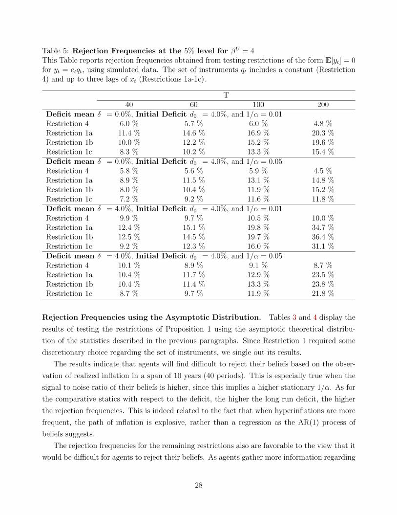
Table 5: Rejection Frequencies at the 5% level for βU = 4This Table reports rejection frequencies obtained from testing restrictions of the form E[yt] = 0for yt = etqt, using simulated data. The set of instruments qt includes a constant (Restriction4) and up to three lags of xt (Restrictions 1a-1c).

T40 60 100 200

Deficit mean δ = 0.0%, Initial Deficit d0 = 4.0%, and 1/α = 0.01Restriction 4 6.0 % 5.7 % 6.0 % 4.8 %Restriction 1a 11.4 % 14.6 % 16.9 % 20.3 %Restriction 1b 10.0 % 12.2 % 15.2 % 19.6 %Restriction 1c 8.3 % 10.2 % 13.3 % 15.4 %Deficit mean δ = 0.0%, Initial Deficit d0 = 4.0%, and 1/α = 0.05Restriction 4 5.8 % 5.6 % 5.9 % 4.5 %Restriction 1a 8.9 % 11.5 % 13.1 % 14.8 %Restriction 1b 8.0 % 10.4 % 11.9 % 15.2 %Restriction 1c 7.2 % 9.2 % 11.6 % 11.8 %Deficit mean δ = 4.0%, Initial Deficit d0 = 4.0%, and 1/α = 0.01Restriction 4 9.9 % 9.7 % 10.5 % 10.0 %Restriction 1a 12.4 % 15.1 % 19.8 % 34.7 %Restriction 1b 12.5 % 14.5 % 19.7 % 36.4 %Restriction 1c 9.2 % 12.3 % 16.0 % 31.1 %Deficit mean δ = 4.0%, Initial Deficit d0 = 4.0%, and 1/α = 0.05Restriction 4 10.1 % 8.9 % 9.1 % 8.7 %Restriction 1a 10.4 % 11.7 % 12.9 % 23.5 %Restriction 1b 10.4 % 11.4 % 13.3 % 23.8 %Restriction 1c 8.7 % 9.7 % 11.9 % 21.8 %

Rejection Frequencies using the Asymptotic Distribution. Tables 3 and 4 display the

results of testing the restrictions of Proposition 1 using the asymptotic theoretical distribu-

tion of the statistics described in the previous paragraphs. Since Restriction 1 required some

discretionary choice regarding the set of instruments, we single out its results.

The results indicate that agents will find difficult to reject their beliefs based on the obser-

vation of realized inflation in a span of 10 years (40 periods). This is especially true when the

signal to noise ratio of their beliefs is higher, since this implies a higher stationary 1/α. As for

the comparative statics with respect to the deficit, the higher the long run deficit, the higher

the rejection frequencies. This is indeed related to the fact that when hyperinflations are more

frequent, the path of inflation is explosive, rather than a regression as the AR(1) process of

beliefs suggests.

The rejection frequencies for the remaining restrictions also are favorable to the view that it

would be difficult for agents to reject their beliefs. As agents gather more information regarding

28

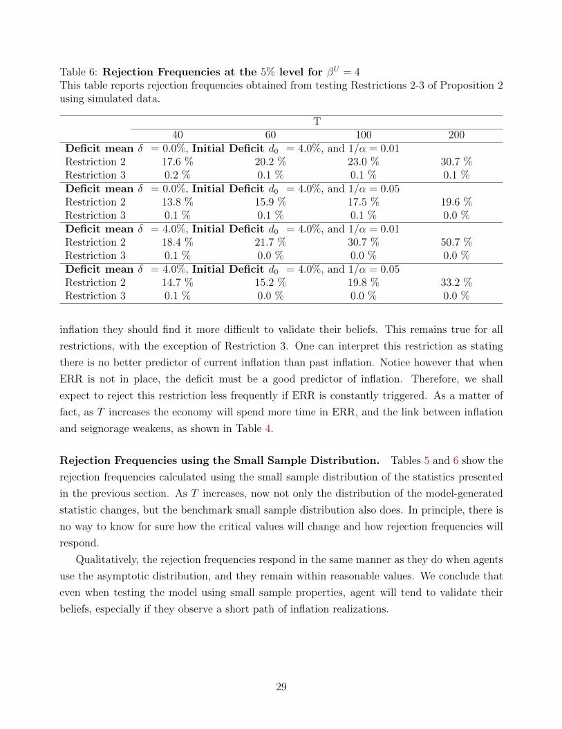
Table 6: Rejection Frequencies at the 5% level for βU = 4This table reports rejection frequencies obtained from testing Restrictions 2-3 of Proposition 2using simulated data.

T40 60 100 200

Deficit mean δ = 0.0%, Initial Deficit d0 = 4.0%, and 1/α = 0.01Restriction 2 17.6 % 20.2 % 23.0 % 30.7 %Restriction 3 0.2 % 0.1 % 0.1 % 0.1 %Deficit mean δ = 0.0%, Initial Deficit d0 = 4.0%, and 1/α = 0.05Restriction 2 13.8 % 15.9 % 17.5 % 19.6 %Restriction 3 0.1 % 0.1 % 0.1 % 0.0 %Deficit mean δ = 4.0%, Initial Deficit d0 = 4.0%, and 1/α = 0.01Restriction 2 18.4 % 21.7 % 30.7 % 50.7 %Restriction 3 0.1 % 0.0 % 0.0 % 0.0 %Deficit mean δ = 4.0%, Initial Deficit d0 = 4.0%, and 1/α = 0.05Restriction 2 14.7 % 15.2 % 19.8 % 33.2 %Restriction 3 0.1 % 0.0 % 0.0 % 0.0 %

inflation they should find it more difficult to validate their beliefs. This remains true for all

restrictions, with the exception of Restriction 3. One can interpret this restriction as stating

there is no better predictor of current inflation than past inflation. Notice however that when

ERR is not in place, the deficit must be a good predictor of inflation. Therefore, we shall

expect to reject this restriction less frequently if ERR is constantly triggered. As a matter of

fact, as T increases the economy will spend more time in ERR, and the link between inflation

and seignorage weakens, as shown in Table 4.

Rejection Frequencies using the Small Sample Distribution. Tables 5 and 6 show the

rejection frequencies calculated using the small sample distribution of the statistics presented

in the previous section. As T increases, now not only the distribution of the model-generated

statistic changes, but the benchmark small sample distribution also does. In principle, there is

no way to know for sure how the critical values will change and how rejection frequencies will

respond.

Qualitatively, the rejection frequencies respond in the same manner as they do when agents

use the asymptotic distribution, and they remain within reasonable values. We conclude that

even when testing the model using small sample properties, agent will tend to validate their

beliefs, especially if they observe a short path of inflation realizations.

29

6. Conclusions

Some countries have been recently confronted with the following policy decision: is it worthwhile

to leave the EMU? In this paper we analyse this policy decision when it involves no government

debt default and the government can not increase its debt level. In this situation leaving the

euro gives a country freedom to monetize its deficit.

We find that the resource to deficit monetization is not a panacea. Given the current

levels of government deficit exiting the euro is likely to lead to hyperinflations. As is well

accepted in policy circles, and as justified by the setup in Marcet and Nicolini (2003), one can

stop hyperinflations with a ERR and lower average seignorage. Therefore, to the extent that

a hyperinflation is a very costly outcome that should be avoided, countries exiting the euro

should find ways to reduce deficits anyway, even outside the EMU.

Another outcome of the paper has been to show how the framework of IR can be used to

perform policy analysis. We just state clearly an assumption on the system of beliefs, we justify

its validity using various criteria spelled out in the text, and we calibrate the parameters of the

belief system. Indeed, the effects of the policy decision will depend on the agents’ expectations

in the model: if agents have RE leaving the euro implies a modest inflation, if agents learn about

underlying inflation as a consequence of their ”near-rational” belief system, rational behavior

will lead to hyperinflations. That the policy outcome depends on how expectations are formed

is an advantadge of our approach, as it highlights that this is a key element in policy decisions,

since policy makers never really know how agents’ expectations will react to a policy change.

This paper hardly exhausts the effects of leaving the euro. Exiting countries could have an

outright debt default; but this alternative has additional costs that should be factored in, other

papers have attempted to measure these costs. Exiting countries may actually not loose access

to debt markets, but even if they have access to debt markets, given their very high current

debt levels it is unlikely they can keep increasing their debt levels much. Exiting countries may

hope that a devaluation brings some growth, this would be beneficial in itself and it would

decrease deficit as a percentage of gdp, but past experience shows that post-devaluation growth

is not always to be had, most of its effect comes through devaluating internal salaries. This

would say, in our model, that lowering the civil servant salaries is a convenient way to implement

austerity and indeed lowering the probability of a hyperinflation, but this is austerity in disguise

anyway. Such lowering of the deficit thanks to inflation can be modelled in by endogeneising

dt to equilibrium inflation, a substantial complication that goes way beyond the current setup.

Another supposed advantage of devaluations is to bring some growth due to lower real wages

and increased international competitiveness of local labor, our model also captures this as a

way to lower seignorage as a percentage of gdp. However, we are silent about other costs and

30

benefits, namely, that lower wages reduce welfare while higher gdp increases welfare. We have

also yet to explore different alternatives for the re-set of beliefs after the euro, consider various

paths for the deficit, calibrate to other countries etc.

In any case the remaining issues can be incorporated in future research that goes vastly

beyond the scope of this paper.

31

A Linearization of the Money Demand Equation

We linearize the individual money demand around a fictitious steady state with no aggregate

uncertainty. In this appendix, we use the notation mjt ≡ M j

t /Pt and πt+1 ≡ Pt+1/Pt. The

linearization boils down to:(1

1− mj

)2

(mjt − mj) = −

(αjt

mjt + ejt+1πt+1

)21

αjt

{Ejt [m

jt − mj] + ejt+1E

jt [π

jt − πj]

}where the tilde variables represent steady state variables. In steady state we must have that

1

1− mj=

αjt

mj + ejt+1π

which also implies that1 + αjt

αjtmj +

ejt+1

αjtπ = 1

Using these two expressions above and rearranging we obtain:

mjt =

αjt

1 + αjt

{1−

ejt+1

αjtEjt [πt+1]

}

which corresponds to the expression in the main text.

B Proof of Proposition 1

If d0 = δ, it is straightforward that π(d0) = π1(δ). Hence, the goal is to show that π(d0) exists

when d0 6= δ. The logic consists in showing that, given d0, one can find a value for π0 so as to

be exactly at π1(dt) in period t, where π1(dt) denotes the solution to the quadratic equation

(18) given the level of seignoriage dt. Notice that such value is well defined for all dt as long as

d0 ∈ D.

Lemma 1 If d0 6= δ, there exists a monotone and bounded sequence of initial conditions {βt}such that for all t, π0 = βt implies πt = π1(dt).

This result indicates that limt→∞ βt is well defined. We denote this limit by π(d0), making

explicit its dependence on the initial value of seigniorage d0. Furthermore, it also indicates

that if π0 = π(d0), then limt→∞ πt = limt→∞ π1(dt) = π1(δ). Hence, the second statement of

Proposition 1 can be viewed as a corollary of Lemma 1. Although the two cases d0 < δ and

32

d0 > δ need to be considered separately, the proof is analogous so we present only the one

corresponding to d0 < δ.

Proof of Lemma 1. The proof is by induction. For the initial step, observe that

π0 = π1(δ) =⇒ π1 = (1− ρ)π1(δ) + ρF(π1(δ), d0) > π1(δ) > π1(d1)

where the first inequality follows from the following property about F :

F(π, d) > π ⇐⇒ π ∈ (π1(d),π2(d))

and the second follows from the fact that d < δ implies π1(d) < π1(δ). On the other hand, we

also have that:

π0 = π1(d0) =⇒ π1 = (1− ρ)F(π1(d0), δ) + ρπ1(d0) < π1(d0) < π1(d1)

Since F is continuous and monotone, it follows that there exists a unique β1 ∈ (π1(d0),π1(δ))

such that if π0 = β1 then π1 = π1(d1).

For the inductive step, suppose there exists βt such that π0 = βt implies πt = π1(dt). Then

it follows that

πt = π1(dt) =⇒ πt+1 = (1− ρ)F(π1(dt), dt) + ρπ1(dt) < π1(dt) < π1(dt+1)

and we have again that

πt = π1(δ) =⇒ πt+1 = (1− ρ)π1(δ) + ρF(π1(δ), dt) > π1(δ) > π1(dt+1)

Hence there exists βt+1 ∈ (βt,π1(δ)) such that π0 = βt+1 implies πt+1 = π1(dt+1). This also

implies that βt+1 > βt for all t, so the sequence is monotone and bounded.

To complete the proof of the proposition, take an arbitrary sequence {πt} that evolves

according to (17) and suppose π0 > π(d0). Two cases need to be considered. First, if π0 ≥max{π1(δ),π1(d0)}, then (17) and the properties of F imply that statement 3 is satisfied.

Second, if π0 ∈ (π(d0),max{π1(δ),π1(d0)}), then the proof of Lemma 1 indicates there exists a

period t in which πt > max{π1(δ),π1(dt)} and therefore (17) and the properties of F again tell

us that statement 3 holds. The proof of the first statement, when π0 < π(d0), follows exactly

the same steps.

33

C Linearization of Equation 15

To linearize Equation 15, we treat πt, πet and πet+1 as different variables. Thus we obtain:

πt =δ

φ− φγπ1(δ)− δdt −

φγπ1(δ)

φ− φγπ1(δ)πet +

φγπ1(δ)

φ− φγπ1(δ)− δπet+1

Rational Expectations implies that, around the low inflation steady state, πet = 0 for all t.

Therefore, the last two terms in the right hand side cancel out and we obtain the equation in

the main text.

D Estimating Inflation Persistence

To calculate inflation paths we use the following system

dt = (1− ρ)δ + ρdt−1 + εt (33)

πt =φ− φγ(ρ2ππt−2 + (1− ρ2π) βt−1)

φ− φγ(ρ2ππt−1 + (1− ρ2π) βt)− dt(34)

= αt−1 + 1 (35)

βt = βt−1 +1

α

(πt−1 − ρππt−2

1− ρπ− βt−1

)(36)

with the initial condition {π−1, d0, α0, β0} = {π1, δ, α,π1}, where π1 is the low inflation steady

state in the RE equilibrium, and α is just a positive integer. We assume that the variance of

the i.i.d shock εt is small enough so that the system remains stable.

We generate N samples of length T for each variable defined in (33)-(36). Let ρπ(N, T ) be

the bootstrap estimate of the persistence of inflation, which is a function of all primitives of the

model, including ρπ and ρ. We allow ρπ 6= ρδ and restrict attention to positive autocorrelation

coefficients. Figure 3 displays ρπ(N, T ) as a function of ρπ. The figure shows that for any ρ,

there is a unique ρπ such that ρπ = ρπ(N, T ). We are interested in those fixed points because

they correspond to the case in which agents are able to estimate ρπ using past data. Since

we proved that in a RE equilibrium, ρ = ρπ, considering ρπ 6= ρδ implies that we are allowing

the persistence of inflation to be biased in a learning equilibrium. The nature of that bias is

portrayed in Figure 4, which plots the fixed point ρ?π = ρπ = ρπ(N, T ) as a function of ρ. The

figure indicates that the bias tends to be negative for low persistence of seigniorage and positive

for high persistence of seigniorage

34

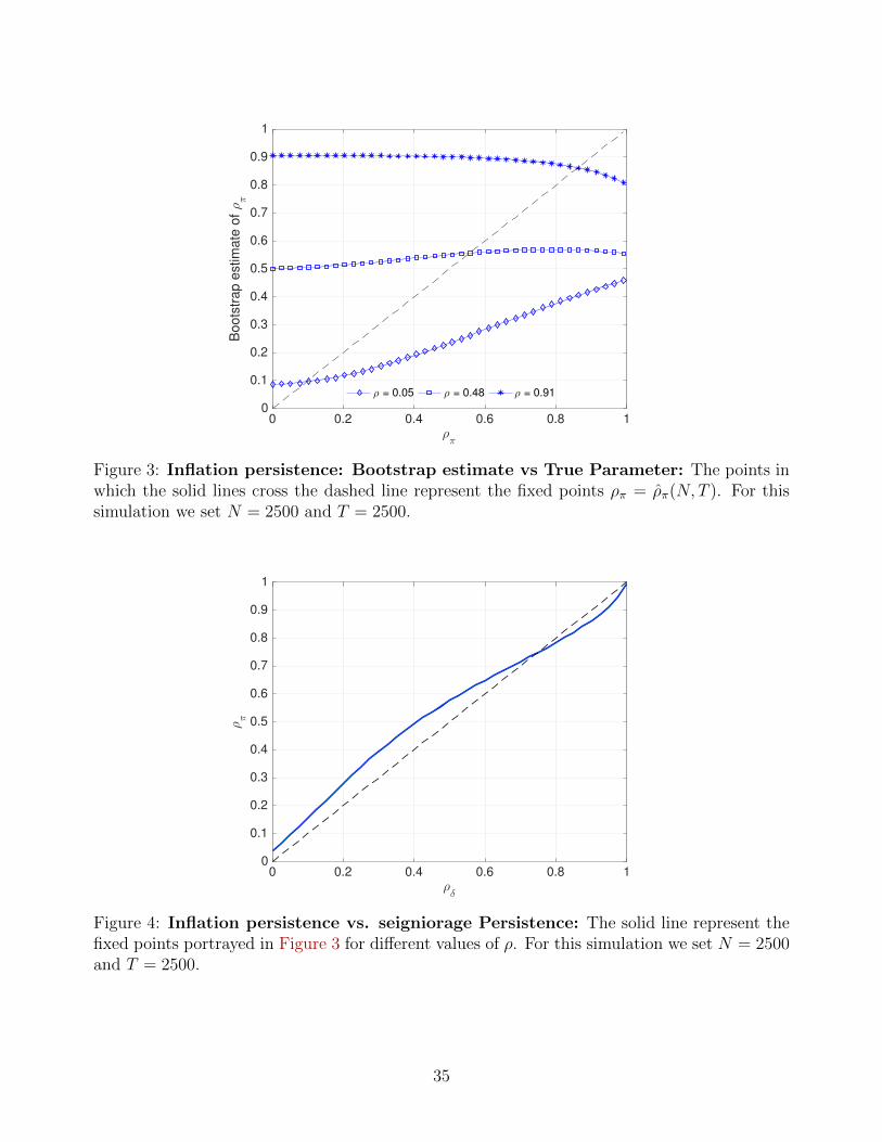
0 0.2 0.4 0.6 0.8 1ρπ

0

0.1

0.2

0.3

0.4

0.5

0.6

0.7

0.8

0.9

1

Boots

trap e

stim

ate

of ρπ

ρ = 0.05 ρ = 0.48 ρ = 0.91

Figure 3: Inflation persistence: Bootstrap estimate vs True Parameter: The points inwhich the solid lines cross the dashed line represent the fixed points ρπ = ρπ(N, T ). For thissimulation we set N = 2500 and T = 2500.

0 0.2 0.4 0.6 0.8 1

ρδ

0

0.1

0.2

0.3

0.4

0.5

0.6

0.7

0.8

0.9

1

ρπ

Figure 4: Inflation persistence vs. seigniorage Persistence: The solid line represent thefixed points portrayed in Figure 3 for different values of ρ. For this simulation we set N = 2500and T = 2500.

35

E Proof of Proposition 2

The proof considers the general formulation in which agents use information about the innova-

tions to the deficit to adjust their expectations regarding future inflation.

Restriction 1. Note that, according to the belief system:

et = π∗t + ψεt + ut −(π∗t−1 + ψεt−1 + ut−1

)= ηt + ψεt − ψεt−1 + ut − ut−1

whereas

dt − ρdt−1 = (1− ρ)δ + εt

so that Restriction 1 holds for i ≥ 2.

Restriction 2. To prove Restriction 2, observe that:

E [(dt − ρdt−1)et] = E [((1− ρ)δ + εt)(ηt + ψεt − ψεt−1 + ut − ut−1)] = ψσ2ε

while

E [(dt−1 − ρdt−2)et] = E [((1− ρ)δ + εt−1)(ηt + ψεt − ψεt−1 + ut − ut−1)] = −ψσ2ε

so that Restriction 2 also holds.

Restriction 3. Note that:

E [etet−1] = E [(ηt + ψεt − ψεt−1 + ut − ut−1)(ηt−1 + ψεt−1 − ψεt−2 + ut−1 − ut−2)]

= −ψ2σ2ε − σ2

u

Now consider the projection of dt − ρdt−1 on et. The projection is given by

Cov [et, dt − ρdt−1]Var [dt − ρdt−1]

(dt − ρdt−1)

36

where

Cov [et, dt − ρdt−1] = Cov [ηt + ψεt − ψεt−1 + ut − ut−1, εt] = ψσ2ε

Var [dt − ρdt−1] = σ2ε

so that the projection is given by ψεt, and the variance of the projection is ψ2σ2ε . Plugging

these results into the right hand side of Restriction 3 delivers:

E [et, et−1] + b′2σ2ε − σ2

u + ψ2σ2ε = −σ2

u < 0

Restriction 4. Since all the perturbation terms have zero expectation, Restriction 4 follows

immediately.

F Model with Assets

The exogenous process is given by sequences (dt, bt) such that b0 = 0, d0 = δ and

dt = (1− ρ)dt−1 + ρδ + ξt

Thus, the true deficit evolves as before, and there is an initial value of assets set to zero.

Consider then the begining of period t, given bt−1, after the draw of dt. Define the new variable:

dt = max{0, dt − (1 + r)bt−1}

which is interpreted as the part of the deficit that can’t be financed with existing assets. Define

also:

bt−1 = max{(1 + r)bt−1 − dt, 0}

which corresponds to the stock of assets left after the deficit is financed. Notice that these

definitions imply that:

dt − bt−1 = max{dt − (1 + r)bt−1, 0} −max{(1 + r)bt−1 − dt, 0}

= max{dt − (1 + r)bt−1, 0} −min{dt − (1 + r)bt−1, 0}

= dt − (1 + r)bt−1

Now, we define a monetary policy rule that avoids deflation. The idea behind this policy rule is

that all money printing is used to finance what is left of the deficit once assets are depleted. In

that case, there are no additional resources created. However, money printing can exceed what

37

is needed to finance the deficit and in that case we assume the extra resources are accumulated

as assets. This amounts to set the law of motion for assets as follows:

bt = max{bt−1, bt−1 + (mt −mt−1 − dt)} (37)

where mt denotes real money balances. In principle, total assets next period should be equal

to end of period assets bt−1 which corresponds to the first term in the max operator. However,

if at zero inflation, real balances were more than enough to cover the deficit after assets were

depleted, then those extra resources are indeed printed and used to purchase additional assets.

To understand the logic of this policy rule, notice that the money demand equation dictates

that:

φ(Pt − Pt−1) = (Mt −Mt−1) + φγ(P et+1 − P e

t )

So, in order to avoid deflation we must have that

Mt −Mt−1 ≥ φγ(P et − P e

t+1) (38)

Deflation becomes an issue only if prices are expected to move down. In that case, the gov-

ernment must print money to avoid deflation. If the money printed exceeds the amount of the

deficit to be financed, then it is used to purchase assets. In other words, if expectations are

such that:

φγ(P et − P e

t+1) > (dt − bt−1)Pt

then according to the government budget constraint, no asset accumulation implies:

Mt −Mt−1 = (dt − bt−1)Pt

so that (38) is violated and deflation ensues. In such a case, assets need to be accumulated to

ensure that φ(Pt − Pt−1) = 0. Since that implies

Mt −Mt−1 > (dt − bt−1)Pt

The excess money printing is used to purchase assets. In other words, the modified government

budget constraint is given by

Mt −Mt−1 + (bt−1 − dt)Pt = btPt

38

which, expressed in real terms, it can be written as:

mt −mt−1

πt+ bt−1 − dt = bt

Evaluated at zero realized inflation, the left hand side of the previous equation corresponds to

the second argument in the max operator of (37). Since it is increasing in πt, if at zero inflation

it is still positive, the excess resources printed are used to purchase extra assets.

39

REFERENCES

• Adam, K., A. Marcet and J.P. Nicolini (2016). ”Stock Market Volatility and Learning”,

Journal of Finance.

• Adam, K., A. Marcet and Johannes Beutel (2016). ”Stock Price Booms and Expected

Capital Gains”, forthcoming American Economic Review.

• Adam K., A. Marcet (2011). “Internal Rationality and Asset Prices” Journal of Economic

Theory.

• David Andolfatto and Paul Gomme (2003), “Monetary Policy Regimes and Beliefs,” In-

ternational Economic Review, 44 (1), 1–30.

• Evans, G. and S. Honkapohja, (2001) Learning and Expectations in Macroeconomics,

Princeton University Press.

• Marcet, A. and T. Sargent, (1989a), ’Convergence of Least Squares Mechanisms in Self-

Referential Linear Stochastic Models’, Journal of Economic Theory 48, 337 - 368.

• Marcet, A. and T. Sargent (1989b), “Least Squares Learning and the Dynamics of Hy-

perinflation” in International Symposia in Economic Theory and Econometrics, vol. 4,

edited by W. Barnett, J.Geweke and K. Shell, Cambridge University Press.

• Marcet, A. and J.P. Nicolini (2003), ”Recurrent Hyperinflations and Learning”, American

Economic Review.

• Roberts, John M., 1997. ”Is inflation sticky?,” Journal of Monetary Economics.

• Stock, J. and M. Watson, 2007. ”Why has U.S. Inflation Become Harder to Forecast?”,

Journal of Money, Credit and Banking.

40