d3 : ground em surveys over 2-d resistivity models d3.1

Geophysics 223 – March 2009

1

D3 : Ground EM surveys over 2-D resistivity models D3.1 Tilt angle measurements

• In D2 we discussed approaches for mapping terrain conductivity. This is

appropriate for many hydrogeology applications where subsurface structure changes slowly with horizontal distance.

• An alternative type of survey was developed for mineral exploration in the early

20th century. A typical Earth model for this type of survey is a very conductive massive sulphide ore body in very resistive bedrock.

• Here the goal is to find the location of the ore body, and then evaluate its size and

depth. D3.1.1 : Measuring the tilt angle

• In this type of survey, the direction of the total magnetic field (HT) is measured. • The receiver coil is rotated until the signal received has the minimum amplitude.

• In this geometry, HT will be parallel to the plane of the search coil.


2

D3.1.2 Example with fixed transmitter and moving receiver

• The transmitter generates an oscillating primary magnetic field with a dipole pattern. Consider an instant in time when the primary magnetic field is oriented from left to right and is increasing with time.

• Time variation in primary magnetic field induces secondary electric currents in

the conductor (shown a shaded vertical box)

• Assume that no secondary electric current is induced in the host rock.

• Secondary current flows in loops within the conductor and generate a dipolar secondary magnetic field.

• The secondary magnetic field is equivalent to a dipole pointing in opposite

direction to the primary magnetic field.

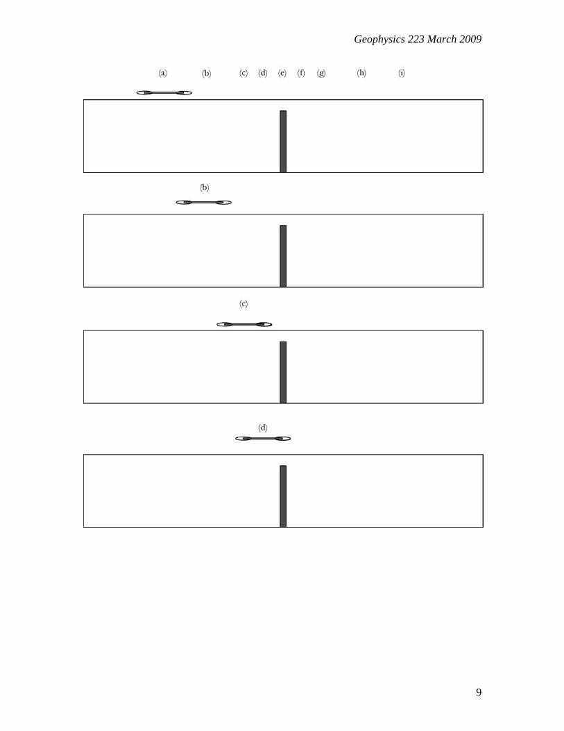
• At each RX location (a) – (g) the primary and secondary magnetic fields are added to give the total magnetic field.

• Simplest magnetic field measurement is to measure the angle between total

magnetic field and the horizontal. This is called the tilt angle and measurement technique is described below.

• Work through this example and you should be able to show that a pattern of

upward , zero and downward tilt angle will be observed from (a) to (g).


3


4

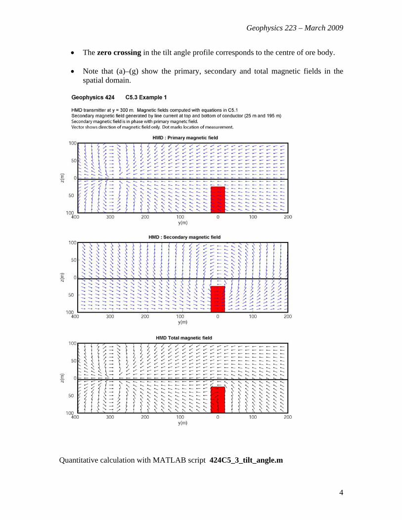
• The zero crossing in the tilt angle profile corresponds to the centre of ore body.

• Note that (a)–(g) show the primary, secondary and total magnetic fields in the spatial domain.

Quantitative calculation with MATLAB script 424C5_3_tilt_angle.m


5

D3.1.3 : Data examples The expected variation in tilt angle (up-horizontal-down) is observed in the total magnetic field over the conductor. Example : Telford 7.94


6

D3.2 : Measurements of amplitude of the total magnetic field Tilt angle measurements such as that shown in D3.1 generally allow us to :

• Locate a conductive anomaly. • Estimate the depth from the width of the tilt angle anomaly.

• Estimate along strike variations in the strength of a conductor since the magnitude

of the conductor will increase the maximum tilt angle observed on a profile However, this type of survey doesn’t yield much quantitative information about the properties of the target. In an alternative field strategy, the magnitude of the total magnetic field (HT) is measured. We will see that this allows us to get quantitative information about the target through the use of characteristic curves (see Geophys 424 for details) Typical systems are initially operated away from a conductor to determine the primary magnetic field, HP. When measurements are made close to the Earth, the total magnetic field is measured and expressed as a percentage change compared to the primary field. For vertical magnetic dipoles (horizontal loops), the survey proceeds with the TX-RX system being moved across the region of interest. This can be with the two loops on a boom carried by the operator (EM31), two loops carried by two field crew (EM34) or with the loops mounted on an aircraft. At each location, the TX is energized and HT measured. The response is plotted at the centre of the TX-RX array and plotted as the percentage change in magnetic field, C = 100 x HT/HP

Two factors can change the amplitude of the total magnetic field measured at the RX:

(1) Changing the TX-RX offset (typical transmitter fields vary as 1/r3) (2) Moving across a buried conductor

Thus changes in the TX- RX offset can mask the effects of basement conductors that we are trying to detect. While the effects of changes in TX-RX offset can be corrected, it is simplest to keep TX-RX offset constant, as in the following example.


7

EM34 traverse across a vertical conductor

• The transmitter (TX) is powered at a single frequency.

• TX and RX are loops connected by a cable and

moved along the profile.

• The loops can be placed in horizontal and vertical configurations.

• The centre of the TX-RX is placed at each location (a) - (g) the total magnetic field

strength is measured. • Again, we will assume that the secondary magnetic field is in phase with the primary

magnetic field. • If TX and RX loops are horizontal, the RX measures the vertical component of the total

magnetic field (Tz). Position (a)

• Primary magnetic field (P) oscillates. • Consider the instant in time when the TX magnetic dipole is pointing upwards. • P passes downwards through the RX coil (this is always the case in this example). • P passes right to left through the conductor. • Generates secondary currents confined to the conductor. • Currents generate secondary magnetic field (S) equivalent to dipole pointing left-to-

right. • S passes downwards (and to right) through RX • P and S in same direction (downwards) at RX. • Tz > Pz

Positions (b) and (c)

• Similar to (a) with signs, but magnitudes of S and T vary. • P passes downwards through the RX coil • Tz > Pz

Position (d)

• Secondary magnetic field (S) equivalent to dipole pointing left-to-right, as in (a)-(c) • S is parallel to the RX loop and there is no conductor-RX coupling. • Tz = Pz

Geophysics 223 March 2009

8

Position (e) • Secondary magnetic field (S) equivalent to dipole pointing left-to-right. • S passes upwards (and to left) through RX • Tz < Pz

Position (f) • P is parallel to the conductor and no secondary field (S) is generated. • No TX-conductor coupling. • Tz = Pz

Position (g)

• Secondary magnetic field (S) equivalent to dipole pointing right-to-left. • P downwards in RX coil • S downwards in RX coil • Tz > Pz

Similar example is shown in the textbook in Figure X-X


9


10


11

Data example : Telford 7.99

• In this example, the total magnetic field is not in phase with the primary field.

Hence the total magnetic field has components that are in-phase (0° difference) and in quadrature (90° difference) with the primary magnetic field.


12

• The relative magnitudes of these two quantities can be used to determine the

conductance and depth of the conductor through the use of characteristic curves (Geophysics 4242, C5.4).

• Generally good conductors have a response that is in-phase with the primary

magnetic field. Thus, the example on the left was for a good conduct

D3.3 VLF (Very Low frequency)

• The final EM method we will consider in this section is the VLF method. It is basically another way of measuring tilt angle. Main difference with the method shown in D3.1 is that a distant radio transmitter is used as an energy source.

• VLF exploration uses large radio transmitters that were built for marine navigation and military communication.

• Some transmitters are still used for submarine communications, while a number of

Russian transmitters have become unreliable or shut down in recent years. • Grimeton VLF transmitter in Sweden is shown above. http://en.wikipedia.org/wiki/VLF_transmitter_Grimeton • Why is the low frequency needed for submarine communication? • The figures below show the areas in which the signals from two North American

transmitters can be detected (McNeill and Labson, 1991). The Cutler transmitter is one of the most powerful in the world (2 MW).


13

Cutler (Maine) Jim Creek (Washington)

• VLF uses radio signals with a frequency around 12-20 kHz. The VLF frequency band is defined as 3-30 KHz and is low in terms of radio communication.

• However, for EM exploration methods, this is a relatively high frequency. The skin

depth equation can be used to estimate penetration depth, and this is generally just a few hundred metres.

• The VLF field is polarized with the magnetic field normal to the TX-RX path.

This is in contrast to magnetotellurics (MT) where the natural EM field generation ensures that signals are arriving from all azimuths.

• A portable, 1 km long, transmitter can be used to give additional VLF signals at the

optimal azimuth.

• However only one frequency is usually available. Why is this a problem?


14

• In the ideal case, the geologic strike of the target points at the TX, which is out of plane in this figure. The magnetic field is parallel to the profile.

(Figures on this page from Geonics EM16 manual)

• More details about the use of the VLF instrument are described in Geophysics

424 section C5.6.1 • The Geonics EM16 is the most widely used EM instrument of all time (according

to www.geonics.com)


15

• Figure above computed with MATLAB script VLF_1.m


16

Example of VLF data from mineral exploration (Telford 7.96)


17

Example of fault mapping with VLF data (Telford 7.97)

• Airborne VLF systems have been developed (Arcone, 1978 and 1979). • Modern VLF instruments automatically measure the amplitudes of both the in-

phase and quadrature components. • VLF is better at mapping horizontal resistivity variations than vertical variations.

d3 : ground em surveys over 2-d resistivity models d3.1

Documents