d3.5 (wp3): sd erlang performance portability · pdf filesd erlang performance portability...

ICT-287510RELEASE

A High-Level Paradigm for Reliable Large-Scale Server SoftwareA Specific Targeted Research Project (STReP)

D3.5 (WP3): SD Erlang Performance Portability

Principles

Due date of deliverable: 31st January 2015Actual submission date: 23rd March 2015

Start date of project: 1st October 2011 Duration: 36 months

Lead contractor: The University of Glasgow Revision: 0.4

Purpose: Design and validate performance portability principles for SD Erlang.

Results: The main results of this deliverable are as follows.

• We have designed and implemented a library which enables Erlang nodes to examine attributes ofother nodes in a distributed system, facilitating the choice of a node which has suitable propertiesto support the spawning of a particular process.

• We have tested this library with a distributed Erlang application, showing that the use of at-tributes can lead to improved performance.

• We have designed and implemented a library which uses an abstract model of communicationtimes between Erlang nodes in order to deploy distributed Erlang applications in such a way asto minimise overheads due to communication delays.

• A careful examination of communication times in several multi-node systems on different scalessuggests that our abstract model provides a good description of real communication latencies.

• Earlier deliverables in D3.5 described SD Erlang, which extends Erlang with a mechanism forpartitioning sets of Erlang nodes into s groups in order to improve communication efficiency. Ourlibraries are not closely coupled with the new features introduced in SD Erlang, but admit easyinteroperability with s groups. The work described here is perhaps best viewed as a complementto SD Erlang rather than an extension of it.

ICT-287510 (RELEASE) 27th March 2015 2

Conclusion: We have designed and implemented libraries which provide methods for implementing dis-tributed Erlang applications in such a way as to obtain efficient performance without requiring detailedinformation about system structure to be coded into the application. We have carried out experimentswhich suggest that our libraries do indeed enable programmers to achieve efficient performance in aportable way.

Project funded under the European Community Framework 7 Programme (2011-14)Dissemination Level

PU Public >PP Restricted to other programme participants (including the Commission Services)RE Restricted to a group specified by the consortium (including the Commission Services)CO Confidential only for members of the consortium (including the Commission Services)


SD Erlang Performance Portability Principles

Contents

1 Executive Summary 3

2 Introduction 32.1 Partner Contributions . . . . . . . . . . . . . . . . . . . . . . . . . . . . . . . . . . . . . 42.2 Relation to other RELEASE technologies . . . . . . . . . . . . . . . . . . . . . . . . . . 4

3 Node attributes 53.1 Defining and propagating attributes . . . . . . . . . . . . . . . . . . . . . . . . . . . . . 5

3.1.1 Attributes . . . . . . . . . . . . . . . . . . . . . . . . . . . . . . . . . . . . . . . . 53.1.2 Propagation strategy . . . . . . . . . . . . . . . . . . . . . . . . . . . . . . . . . . 63.1.3 Attribute server . . . . . . . . . . . . . . . . . . . . . . . . . . . . . . . . . . . . 6

3.2 Populating the attribute table . . . . . . . . . . . . . . . . . . . . . . . . . . . . . . . . . 63.2.1 Configuration File . . . . . . . . . . . . . . . . . . . . . . . . . . . . . . . . . . . 63.2.2 Built-in attributes . . . . . . . . . . . . . . . . . . . . . . . . . . . . . . . . . . . 7

3.3 Querying attributes and choosing nodes . . . . . . . . . . . . . . . . . . . . . . . . . . . 83.3.1 Querying attributes . . . . . . . . . . . . . . . . . . . . . . . . . . . . . . . . . . 83.3.2 Choosing nodes . . . . . . . . . . . . . . . . . . . . . . . . . . . . . . . . . . . . . 8

3.4 Experimental validation . . . . . . . . . . . . . . . . . . . . . . . . . . . . . . . . . . . . 93.4.1 Multilevel ACO . . . . . . . . . . . . . . . . . . . . . . . . . . . . . . . . . . . . . 93.4.2 Attribute-aware ML-ACO . . . . . . . . . . . . . . . . . . . . . . . . . . . . . . . 10

3.5 Discussion . . . . . . . . . . . . . . . . . . . . . . . . . . . . . . . . . . . . . . . . . . . . 113.5.1 Attribute Propagation Strategy . . . . . . . . . . . . . . . . . . . . . . . . . . . . 113.5.2 Reliability . . . . . . . . . . . . . . . . . . . . . . . . . . . . . . . . . . . . . . . . 123.5.3 Attributes and s groups . . . . . . . . . . . . . . . . . . . . . . . . . . . . . . . . 12

4 Communication Distances 134.1 Metric and ultrametric spaces . . . . . . . . . . . . . . . . . . . . . . . . . . . . . . . . . 134.2 Trees and ultrametric spaces . . . . . . . . . . . . . . . . . . . . . . . . . . . . . . . . . 14

4.2.1 Implementation . . . . . . . . . . . . . . . . . . . . . . . . . . . . . . . . . . . . . 154.3 Comparing the model with reality . . . . . . . . . . . . . . . . . . . . . . . . . . . . . . 16

4.3.1 Empirical validation . . . . . . . . . . . . . . . . . . . . . . . . . . . . . . . . . . 164.3.2 Cluster Analysis . . . . . . . . . . . . . . . . . . . . . . . . . . . . . . . . . . . . 17

4.4 Measurements . . . . . . . . . . . . . . . . . . . . . . . . . . . . . . . . . . . . . . . . . . 194.4.1 Eight core machine . . . . . . . . . . . . . . . . . . . . . . . . . . . . . . . . . . . 204.4.2 Forty-eight core machine . . . . . . . . . . . . . . . . . . . . . . . . . . . . . . . . 214.4.3 Departmental network . . . . . . . . . . . . . . . . . . . . . . . . . . . . . . . . . 234.4.4 EDF’s Athos cluster . . . . . . . . . . . . . . . . . . . . . . . . . . . . . . . . . . 24

4.5 Determining cluster structure automatically . . . . . . . . . . . . . . . . . . . . . . . . . 294.6 Experimental evaluation . . . . . . . . . . . . . . . . . . . . . . . . . . . . . . . . . . . . 33


5 Discussion 355.1 Practical issues . . . . . . . . . . . . . . . . . . . . . . . . . . . . . . . . . . . . . . . . . 35

5.1.1 Concrete and abstract bounds . . . . . . . . . . . . . . . . . . . . . . . . . . . . . 355.1.2 Conflicting constraints . . . . . . . . . . . . . . . . . . . . . . . . . . . . . . . . . 355.1.3 Avoiding clashes when spawning processes . . . . . . . . . . . . . . . . . . . . . . 355.1.4 Fault-tolerance . . . . . . . . . . . . . . . . . . . . . . . . . . . . . . . . . . . . . 355.1.5 Dynamic changes to network structure . . . . . . . . . . . . . . . . . . . . . . . . 36

6 Conclusions 36

A Appendix: Querying attributes in a real system 36


1 Executive Summary

We consider the problem of deploying distributed Erlang applications on large heterogeneous clustersof machines so as to achieve good performance in a portable way.

We propose two methods which programs can use to achieve this. Firstly we look at the notionof node attributes, which allow an application to examine the properties of remote nodes in order toselect one on which to spawn a process. Secondly, we consider a notion of communication distance:this provides a model of communication latencies in a network, enabling an application to select nodesin such a way as to facilitate efficient communication.

We have developed libraries which implement these ideas, and have performed some experimentalvalidation. For attributes, we have modified one of our existing benchmarks to use attributes in orderto spawn remote processes on suitable nodes, and have shown that doing so provides considerablybetter performance than random node selection. For communication distances, we have carried outa detailed empirical investigation of communication times on a number of systems on different scales,and our results suggest that in general our model gives a simple but effective description of hierarchiesof communication times in real systems.

The techniques described here are complementary to the s group concept described in earlier WP3deliverables [REL12a, REL13a, REL13b, REL14]. S groups partition the nodes in a distributed Erlangsystem so as to reduce the number of inter-node connections, and hence the amount of communicationrequired to keep nodes informed about the state of the system. The libraries described in the presentdocument facilitate node selection from arbitrary sets of nodes: they can thus be used either in astand-alone manner, or if s groups are in use they can be used to select nodes from particular s groups.

2 Introduction

When deploying applications written in Erlang (or some other language) on large distributed systems,difficulties emerge which do not arise in smaller systems. For example:

• The individual machines comprising the system may not all be the same: they may have differingamounts of RAM, different software installed, and so on.

• Communication times may be non-uniform: it may take considerably longer to send a messagefrom machine A to machine B, than it does to send a message from machine C to machine D.This will be particularly important in large distributed applications, where communication timesmay begin to exceed the time required for individual processes to carry out their computations,and hence will start to dominate overall execution time.

These factors will make it difficult to deploy applications, especially in a portable manner. A program-mer may be able to use system-specific knowledge to decide where to spawn processes so as to enablean application to run efficiently, but if the application is then deployed on a different system (or if thestructure of the system changes as nodes fail or new nodes are added) this knowledge could becomeuseless. This problem could become especially pernicious if the deployment strategy is built into thecode of the application.

In order to address these difficulties, we propose a notion of semi-explicit placement, where the pro-grammer selects nodes on which to spawn processes based on run-time information about the propertiesof the nodes (and of the overall system) rather than selecting nodes explicitly based on system-specificknowledge. For example, if a process performs a lot of computation one would like to spawn it on anode with a lot of computation power, or if two processes are likely to communicate a lot then it wouldbe desirable to spawn them on a pair of nodes which communicate quickly.


We have implemented two Erlang libraries which address the problems outlined above. The firstdeals with node attributes, which describe the properties of individual Erlang nodes (and the physicalmachines on which they run). The second deals with a notion of communication distances which modelsthe communication times between nodes in a distributed system.

We describe the theory, implementation, and validation of these ideas in the next two sections, thendiscuss some issues which our initial experiences have brought to light.

2.1 Partner Contributions

The principal contributor to the work described here was the University of Glasgow. EDF providedaccess to their Athos cluster, and there was considerable interaction with them regarding the usage andbehaviour of the cluster. The University of Uppsala also provided access to their TINTIN cluster, butour use of this was minimal. Ericsson and Uppsala provided useful help with in relation to the behaviourof various Erlang VM versions; the details of this are not discussed here (see [REL15c] instead), butthis was helpful in interpreting our experimental results.

2.2 Relation to other RELEASE technologies

SD Erlang. Earlier deliverables [REL12a, REL13a, REL13b] have described s groups, which partitionthe nodes in a distributed Erlang system and improve scalability by restricting the scope of “global”operations. The concepts we describe here are closely related, since the s group(s) to which a nodebelongs are another factor which may influence its selection as a target for spawning a particular process.In fact, in earlier documents we envisaged a single choose nodes function which would allow one toselect nodes based on s groups, attributes, or distances (or a combination of these): see [REL13a, §4].

Our present (preliminary) implementation has diverged somewhat from our earlier proposals, andwe have not integrated the attribute and distance properties with s groups. This has the advantage thatour standalone libraries can be used with any version of Erlang/OTP (not just the RELEASE version),but has the disadvantage that one might now need to call functions from several different libraries toselect a node, adding some overhead. For example, we might ask for a list of all the nodes in a particulars group, then call another function to obtain a subset of these satisfying some distance criterion, thencall another function to select nodes from the new subset which have particular attributes; a singleintegrated choose nodes function would allow one to do all of these things with a one function call.We have not yet used all of the selection features (s groups, attributes, distances) in combination,so this has not been problematic; however, a fully realistic design would require some more thought.See §3.5.3 for more on this.

WombatOAM. WombatOAM [REL12b, REL13c, REL15a] is a (closed-source, commercial) productof Erlang Solutions Ltd which is used for deploying and managing Erlang applications on large dis-tributed systems, either physical or cloud-based. Wombat can collect so-called metrics from the nodeswhich it is managing [REL12b, §4.2.2]. Metrics are properties of Erlang VM: for example, sizes of runqueues, numbers of processes, numbers of atoms, and so on. There are about 90 built-in metrics, andusers can define their own, for example by using the Folsom [Bou] or Exometer [Feu] libraries. Wom-bat uses metrics for monitoring the behaviour of Erlang nodes: someone using Wombat to manage adistributed Erlang application can ask for information about metrics, plot graphs of them, and so on.

Wombat’s metrics are closely related to the attributes described below, but our attribute values aremade available to other nodes in order to assist with process placement; in contrast, Wombat collectsmetrics and does not make them easily available to the nodes which it is managing.

We have implemented a few built-in attributes for demonstration purposes, but we have left thegeneral process of defining attributes open-ended so that they could be defined by a programmer or


supplied in the form of a library. Wombat’s metrics would be a good source of useful attributes, butwe have as yet made no attempt to interface our attribute library with Wombat.

SD-Mon. The SD-Mon tool developed at the University of Kent [REL15b] provides facilities formonitoring running SD Erlang systems; among other things, it can collect statistics about the flowof messages between nodes. This information could be useful in understanding the “communicationdistances” between nodes which forms an important part of §4 below. We hope to investigate thisfurther in future work.

3 Node attributes

3.1 Defining and propagating attributes

This section describes an implementation of a library for managing attributes for Erlang nodes, and alsoa choose nodes function which makes use of these attributes to select nodes with certain properties.The implementation is contained in a library called attr.

3.1.1 Attributes

There are a large number of properties which may be of interest when selecting an Erlang node onwhich to spawn a process. We divide these into static and dynamic attributes.

Static attributes describe properties of a node which are not expected to change during the lifetimeof an Erlang application. Some possibilities are

• The operating system type and version.

• The amount of RAM available.

• The number of cores used by the VM.

• Availability of other hardware features such as specialised floating point units or GPUs.

• Availability of software features, such as particular libraries. A specific example of this is thatthe Erlang crypto library requires a C library from OpenSSL versions later than 0.9.8. We haveused a number of platforms where sufficiently recent OpenSSL versions have not been installed,and this leads to run-time failures of Erlang applications which use functions from crypto.

• Access to shared filesystems. One reason for this might be that an application may wish to useErlang’s DETS tables (which are are stored on disk), and thus if a number of VMs all wish toaccess the same table then they must all be able to access the same filesystem. This may bepossible if all of the VMs are running in machines in the same cluster, but not if they’re runningon different clusters.

On the other hand dynamic attributes describe properties which are expected to vary during programexecution; for example:

• The load on the physical machine as a whole (including other users’ processes).

• The number of Erlang processes running in the VM.

• The amount of memory which is currently available.

• Whether a particular type of Erlang process is currently running on the machine. One mightwant to spawn a process on a VM which is already running some other type of process, or onemight wish to avoid competing with a CPU-hungry process.


3.1.2 Propagation strategy

One of the fundamental properties of attributes is that (in our use-cases at least) they should beavailable to other VMs, so that a suitable machine can be selected to spawn a process which has specialrequirements. The question then arises of how attributes should be propagated through a network.The technique adopted in the present (prototype) implementation is to equip each Erlang node with asmall server which maintains a database of attributes. When a process wishes to select another nodeto spawn a process on, it queries the nodes it’s interested in and asks for the values of the attributesinvolved in the selection criterion. The servers on these nodes return the attribute values to the originalnode, which then makes a choice according to the information which it has received. We will discussthe merits and demerits of this approach later on, and suggest extensions and alternatives.

3.1.3 Attribute server

Attributes are stored in an attribute table on each node. Our current implementation uses an ETStable for this, although Erlang’s recently-introduced maps might be a more lightweight alternative.The attribute table contains two types of entry:

• Static attributes are stored as name-value pairs, for example {num_cpus, 4} or {kernel_version,{3,11,0,12}}. The first entry is an Erlang atom, and the second is an arbitrary Erlang term(typically a number, string, or tuple).

• Dynamic attributes are represented by tuples of the form {dynamic, {M,F}}. Here M is thename of a module and F is the name of a zero-argument function in M . When a dynamicattribute is looked up, the function M:F () is evaluated and its result is returned as the value ofthe attribute.

We also allow dynamic attributes of the form {dynamic,{M,F,A}} where A is a list of arguments.

The attribute table is managed by a process which is registered with the local name attr server.Remote nodes can request information about attributes by evaluating a term of the form

{attr_server, Node} ! {self(), {report, Key, AttrNames}}.

Here AttrNames is a list of attribute names and Key is an Erlang reference (see make_ref/0) which isused to match responses with requests. When the server receives a request of this form, it looks up allof the specified attributes and sends back a message containing the attribute names and their values. Ifan attribute cannot be found, or if there is some problem in evaluating a dynamic attribute, the atomundefined is returned as the value of the attribute.

3.2 Populating the attribute table

3.2.1 Configuration File

How do the attributes get into the attribute table? The attribute server can be started by callingattr:start(ConfigFile) where ConfigFile is a string containing the name of a configuration file,which in turn contains an Erlang list of attributes. For example, a configuration file might contain

[{num_cpus, 4},

{hyperthreading, 2},

{cpu_speed, 2994.655},

{mem_total, 3203368},

{os, "Linux"},


{kernel_version, {3,11,0,12}},

{num_erlang_processes, {dynamic, {erlang, system_info,

[process_count]}}

].

The final entry here is a dynamic attribute which evaluates erlang:system_info (process_count):this returns the total number of processes existing on the node at the current point in time.

We also provide functions insert_attr(attrname, AttrValue), update_attr(attrname, AttrValue)

and delete_attr(attrname) which can be used to modify attributes during program execution; onespecific use of these would be for a node to advertise the fact that it is running a particular type ofprocess (but see §5.1.4 below for a discussion of a potential problem with this strategy).

This scheme is completely extensible. Users can define arbitrary static and dynamic attributes. Fordynamic attributes, they can even use functions from their own libraries (although caution should beexercised here since an attribute which takes a long time to calculate could slow things down; also, anattribute whose evaluation never terminates would cause the server to become locked up).

Discovering static attributes automatically. Many static properties of the system can be discov-ered automatically, for example by examining system files. The attr library includes a mechanism forspecifying such attributes in the configuration file by means of terms of the form {automatic, {M,F}}

and {automatic, {M,F,A}}, where the given functions are evaluated once just after the configurationfile is read, with the resulting values being stored in the attribute table in the same way as normalstatic attributes.

Non-instantaneous attribute values. When a dynamic attribute is queried, the related functionis called and the result is returned. This will typically return the value of the attribute at a particularmoment, whereas in some cases it might be desirable to have a value averaged over some time period.For example, it might be useful to know the average number of Erlang processes running on a nodeduring the last five minutes. In some cases, the attribute may in fact be implemented by callingsome system function which already performs such averaging: for example, see the built-in loadavg15

function described in the next section. In other cases, a user might want to implement their own non-instantaneous attributes. This can in fact be done using the automatic attributes described above:one could specify a function which would spawn a process which would then run at regular intervalsand use the update_attr function to modify the current value of the relevant attribute. This is nothow we intend automatic attributes to be used, and it might be worth extending the attr library toinclude explicit support for non-instantaneous attributes.

3.2.2 Built-in attributes

As mentioned above, many system properties can be discovered automatically, for example by examiningfiles in the proc filesystem on Linux, or by using Erlang functions such as erlang:system_info,erlang:statistics, or functions in the os Erlang kernel library.

As an experiment, we have implemented a small number of useful attributes of this form which areautomatically loaded when the attribute server is started. Most of these are kept in a library calleddynattr. The built-in attributes are loaded before the contents of the configuration file, and will beoverridden by user-defined versions. The attribute server can also be started without a configurationfile, by calling attr:start(); in this case, only the built-in attributes will be loaded. One can also callattr:start(nobuiltins) or attr:start(nobuiltins, ConfigFile) to omit the built-in attributes.

The current built-in attributes are described in Tables 1 and 2.


Attribute name Value

os_type This calls os:type(), which returns a pair such as {unix, linux} giving the family(either unix or win32) and type of the operating system.

os_version This calls os:version() which will return a tuple or string containing the OSversion.

otp_release This calls erlang:system_info(otp_release) to get the OTP version.vm_num_processors This calls erlang:system_info(logical_processors_available) to get the

number of processors available to the VM. This may be less than the total numberof processors on the physical machine if the VM is restricted to use some subset ofthe processors.

mem_total Total memory on the system (in kB), found in /proc/meminfo.

Table 1: Built-in static attributes

Attribute name Value

cpu_speed Current speed (in GHz) of the first CPU , as found in /proc/cpuinfo.mem_free Current free memory (kB) , from /proc/meminfo.loadavg1 System load average over last minute, from /proc/loadavg. The value is a float

between 0 and 1: see man proc and man uptime for details.loadavg5 Load average over last 5 minutes.loadavg15 Load average over last 15 minutes.kernel_entities Numbers of Linux scheduling entities (processes/threads), from /proc/loadavg.

This returns a pair {R,E}, where R is the number of currently runnable entitiesand E is the total number of entities on the system.

num_erlang_processes Number of Erlang processes currently existing on the VM, fromerlang:system_info(process_count).

Table 2: Built-in dynamic attributes

This is just a sample implementation for experimental purposes. However, it does show that quitea large range of properties can be expressed by attributes. Note however that many of the attributes(in particular system load) are found by consulting files in the Linux proc filesystem. This definitelywon’t work on Windows (you’ll get undefined if you try to look up these attributes), and perhaps noton other Unix implementations where the precise format of the files may differ.

3.3 Querying attributes and choosing nodes

3.3.1 Querying attributes

The attr library also contains a function called request_attrs which can be used to query a list ofnodes for the values of specified attributes. This is done by a call of the form request_attrs (Nodes,

AttrNames) where Nodes is a list of node names and AttrNames is a list of attribute names, for example

request_attrs([vm1@osiris, vm1@bwlf01, vm2@bwlf02],

[loadavg1, cpu_speed])

The function returns a list of the form [NodeName, [{AttrName, AttrValue}]].

3.3.2 Choosing nodes

We have used the request_attrs function to implement a simple choose_nodes function. This takesa list of nodes and a list of predicates which those nodes must satisfy. For example:


choose_nodes(Nodes, [{cpu_speed, ge, 2000},

{loadavg5, le, 0.6},

{vm_num_processors, ge, 4}])

The function calls request_attrs to get the values of the required attributes on the specified machines,then evaluates the predicates (discarding attributes whose values are undefined) and returns the subsetof the nodes for which all of the predicates are satisfied. See Appendix A for a sample session on theHeriot-Watt network.

We currently provide two types of predicates. The first carries out comparisons of attribute valuesagainst constants: {AttrName, op, Const}. We currently have the usual six comparison operators:eq, ne, lt, le, gt, and ge. These correspond to the Erlang operators ==, /=, <, =<, >, and >=,respectively. These operators can compare any two Erlang terms, although you sometimes have to becareful; for example, [1,2,3,4] < [1,2,4] but {1,2,3,4} > {1,2,4}. Note also that we’ve used ==

and /= instead of =:= and =/= so that we get the expected results when comparing floats and integers.The second type of predicate checks boolean values: we can say {AttrName, true} and {AttrName,

false} (or {AttrName, yes} and {AttrName, no}).This is a fairly minimal predicate grammar, implemented here as a proof of concept. It should

suffice for many purposes, but it wouldn’t be hard to extend it (by adding disjunction, for example) ifnecessary.

3.4 Experimental validation

As a validation experiment, we ran a modified version of our multilevel Ant Colony Optimisationapplication, ML-ACO. This is described in some detail in [REL15c, §3.2.2], but we recapitulate herefor convenience.

3.4.1 Multilevel ACO

The ML-ACO application is structured as a tree: see Figure 1. There is a single master node M , and anumber of submaster nodes S and colony nodes C. The colony nodes independently construct solutionsto a certain problem, and after a certain number of iterations report their solutions to a submasternode on the level above. Each submaster chooses the best solution from its children and passes thatto the level above, and so on. Eventually, the master node selects the best solution from its children,which is the best solution from among all of the colony nodes. This solution is then sent back down thetree to the colony nodes, which use it to guide their search for new improved solutions. This process isrepeated a number of times, after which the master reports its current best solution and the applicationterminates.

M

S S S

S S S

C C C C C C C C C

Figure 1: Multilevel ACO


The colony nodes perform a considerable amount of mathematical computation (and themselves havea number of ant processes constructing solutions concurrently), but the master and submaster nodesdon’t do much work. It would therefore seem reasonable to run colonies on VMs with lots of processorsand master and submaster nodes on colonies with fewer processors.

3.4.2 Attribute-aware ML-ACO

We modified ML-ACO so that it used attributes to spawn submasters on small Erlang nodes (at most4 processors) and colonies on large ones (more than 4 processors). This was run on 256 compute nodesin EDF’s Athos cluster; three machines each had 24 small VMs running (one pinned to each core) andthe other 253 had a single large VM. We ran the modified ML-ACO version with the VMs presentedin random order, gradually increasing the number of ants from 1 to 80 ants. For each number of ants,the program was run 5 times using attributes for placement and 5 times without attributes (processeswere just spawned on nodes in the random order in which they were presented to the application).

Figure 2 shows the resulting execution times, and we see that the program performs substantiallybetter when attributes are used for placement. This is unsurprising, since when attributes aren’t used,colony nodes will often be placed on Erlang VMs which are only using one core instead of 24. Thesecolonies will take much longer to execute than ones on VMs using lots of cores, and this slows theentire program down. This is confirmed by Figure 3, which shows the ratio of execution times withoutattributes to those with attributes. For small numbers of ants, the performance of the attribute-unawareversion is similar to the attribute-aware version, but the ratio become progressively worse as the numberof ants (and hence the number of concurrent processes) in the VM increases. We expect that the ratiowould asymptotically approach 24 with very large numbers of ants, but we did not have time to checkthis.

●●

●

●●

●● ●

●

●●

● ●

●●

● ●●

●●

● ●

●● ●

●

●●

● ●

●●

● ●●

●

●

●●

●●

●●

●

●

●●

●●

●●

●

● ● ●

●●

●

●●

●

●●

●●

● ●

●

●●

●●

●●

●

●● ●

●●

0 20 40 60 80

1020

3040

50

Number of ants

Exe

cutio

n tim

e (s

)

● ● ● ● ● ● ● ● ● ● ● ● ● ● ● ● ● ● ● ● ● ● ● ● ● ● ● ● ● ● ● ● ● ● ● ● ● ● ● ●● ● ● ● ● ● ● ● ● ● ● ● ● ● ● ● ● ● ● ● ● ● ● ● ● ● ● ● ● ● ● ● ● ● ● ● ● ● ● ●

●

●

Not using attributesUsing attributes

Figure 2: Execution times with and without attributes


●

●●

●●

●

● ●

●

●●

●●

●

●

●●

●

● ●

● ●

●●

●●

●●

●

●●

●

●●

● ●

● ● ●

●

●

● ●●

●

●

●

●

●

●

●

●●

● ●

●

●

●●

●

●

● ●●

●● ●

●●

●

●

●

●

●●

● ●

●

●●

0 20 40 60 80

24

68

Number of ants

Tim

e w

ithou

t attr

ibut

es

Tim

e w

ith a

ttrib

utes

Figure 3: Ratio of execution times

This is admittedly a rather artificial example, since the effect of introducing small VMs is quite pre-dictable. However, it does demonstrate that the use of node attributes can improve performance in aheterogeneous network, and that this can be done without any information about the network beingcoded into the program. Ideally we would have tested the use of attributes with a large and complexprogram such as Sim-Diasca, but unfortunately time constraints precluded this.

3.5 Discussion

3.5.1 Attribute Propagation Strategy

We have adopted a very simple strategy here: when a node wants to know the value of an attribute onanother node, it just asks for it. Another approach would be to have nodes broadcast their attributesto all the other nodes they’re connected to. Indeed, in [REL12a, §6.2] and [REL13a, §4] we describeda design and an initial implementation of basic attributes using this strategy; however, our presentapproach seems to have several advantages:

• Information is only transmitted when it’s required, and only to nodes that require it. It’s pos-sible that in a real system, only a limited number of nodes would actually be spawning remoteprocesses, and they’re the only ones which would need to receive attribute information. Perhapsone could have a model where nodes have to register to receive attribute information (and whenwe’re considering s groups we could imagine each group having a single node which collects anddistributes attribute information).

• Only those attributes which are required are computed and transmitted. We presumably don’twant thousands of nodes broadcasting their load average to everyone once a minute if it’s seldomrequired.


• In this scheme, information about dynamic attributes is always fresh. If attribute information hasto be broadcast then it will sometimes be out of date unless you’re broadcasting it regularly, whichmight lead to too much network activity. Also, some overhead is incurred in finding the valueof dynamic attributes, and this would be adding extra load to machines if we had to calculatedynamic attributes at frequent intervals.

On the other hand, there are some disadvantages to asking for attributes when you need them:

• If we’re spawning a lot of processes, we might be making a lot of requests to the attribute servers,adding load to the target machines. There’s a tension between this factor and the danger offlooding the network with too many broadcast attributes.

• If there’s a lot of latency in the network (or just between the machine which is making therequest and a single member of the list of machines it’s querying) then request_attrs andhence choose_nodes will take a long time every time it’s called. This could slow things downconsiderably in comparison to the case where information is broadcast regularly.

It may be possible to find some middle ground by having request_attrs cache responses (in an ETStable, for example). Once a static attribute has been retrieved once, it would never be necessary to askfor it again (although one might end up with attribute information belonging to defunct machines, soit might be worth invalidating all of the static attributes once every few hours). Dynamic attributescould be saved with a timestamp, and if they’ve been in the cache too long then we could ask for theirvalue again. The time for which an attribute is valid could even vary with the attribute: we probablywant to discard the 1-minute load average quite quickly, but we could keep the 15-minute load averagefor a while.

Given more time, we would have liked to implement a system where attributes are broadcast acrossthe network as well, and to see how this method compares with the one we have already implemented.It is possible that the second approach would be more effective in certain situations, but this woulddepend on the properties of the application.

3.5.2 Reliability

The present implementation is fairly simplistic, and makes no pretence to reliability. If a node’sattribute server crashes for some reason then there’s no attempt to restart it. There are also problemsin querying such nodes. At the moment, request_attrs times out if it has to wait too long: if nothinghappens for 5 seconds after receiving its most recent message, it just times out and returns whateverattributes it’s already received. If an attribute server has gone down then request_attrs will take atleast 5 seconds every time it requests information from a list of nodes which contains a bad one. Onthe other hand, timing out runs the risk of missing a response from a live node which is taking a longtime to respond.

See §5.1.4 below for some related points.

3.5.3 Attributes and s groups

In earlier deliverables ([REL12a, REL13a, REL13b, REL14]), , we have described and implementeds groups, which are important for improving scalability of distributed Erlang applications.

In this document we haven’t considered the interaction of node attributes and s groups; however itshouldn’t be too difficult to integrate the two. The current choose_node function takes a list of Erlangnodes as its first argument, so one can easily supply it with the members of an s group, obtained usingthe s_group:own_nodes function for example. One could modify attr:choose_node to take an s groupname as a parameter, but this would make it quite tightly coupled to the s_group library, which is not


part of the standard Erlang/OTP distribution; our current attr library can be used with any Erlangversion.

4 Communication Distances

In many modern distributed computer installations, the inter-node communication infrastructure hassome kind of hierarchical structure. Within a particular organisation, machines in a cluster may beconnected together by a high-speed network, and this network may be in turn be connected to othermachines within the organisation via a network with slower communication. If the network spansseveral sites in different geographical locations, then communication between sites may be slower still.Connecting to machines in a different organisation may introduce further delays.

On a smaller scale, communication between processing units within an SMP machine may be sim-ilarly hierarchical: inter-processor communication rates may depend on the level of cache which twoprocessors share, or whether the processors are located on the same socket.

In this section we describe an implementation of an abstract model of communication times whichcan be used for process placement in systems with this type of hierarchical communication structure.We use an idea of P. Maier [MST14].

Suppose we have a collection of Erlang nodes. A useful way to think about inter-node communicationtimes is to think of the nodes as points in a space and to regard communication times as distancesbetween these points. An appropriate mathematical model is the notion of a metric space (see [HS65,6.12] or [Rud76, 2.15], for example).

4.1 Metric and ultrametric spaces

Definition. A metric space is a set X together with a function

d : X ×X → R+ = {x ∈ R : x ≥ 0}

such that, for all x, y, z ∈ X,

(i) d(x, y) = 0 if and only if x = y

(ii) d(x, y) = d(y, x)

(iii) d(x, z) ≤ d(x, y) + d(y, z)

The inequality (iii) is called the triangle inequality. If we replace (iii) with

(iii′) d(x, z) ≤ max{d(x, y), d(y, z)}

then we obtain the definition of an ultrametric space [Kra44] (and (iii′) is called the ultrametric in-equality). It is not hard to see that every ultrametric space is a metric space.

Metric spaces give a very general model of distances, and admit generalisations of many conceptsfrom standard geometry. One specific concept we will make use of is the closed disc.

Definition. Let X be a metric space. For x ∈ X and r ∈ R+, the closed disc of radius r with centrex is

D(x, r) = {y ∈ X : d(x, y) ≤ r}.


4.2 Trees and ultrametric spaces

Given a tree (with an arbitrary amount of branching), we can define a metric (in fact, an ultrametric)on its set of leaves by

d(x, y) =

{0 if x = y

2−`(x,y) if x 6= y.

where `(x, y) is the length of the longest path which is shared by the paths from the root to x and y:see Figure 4. We leave it as an exercise to show that d is in fact an ultrametric.

h i j

e f ga b c d k l m

(a) d(b, c) = 14

h i j

e f ga b c d k l m

(b) d(b, g) = 12

h i j

e f ga b c d k l m

(c) d(b, k) = 1

Figure 4: Distances between nodes


Figure 5 shows what closed discs look like with respect to the metric d. This diagram suggests whythis particular metric might be useful for studying communication distances: given a (computing)node in some hierarchical communication system, the various closed discs contain nodes which are inthe same subclusters at various levels, and hence which might be expected to have similar inter-nodecommunication times.

h i j

e f ga b c d k l m

(a) D(b, 0.3)

h i j

e f ga b c d k l m

(b) D(b, 0.8)

h i j

e f ga b c d k l m

(c) D(b, 1)

Figure 5: Closed discs around node b

4.2.1 Implementation

We have implemented a simple Erlang library which carries out calculations using ultrametric distances.It takes as input a tree (represented as an Erlang term) which describes the structure of a network ofErlang VMs, and then uses closed discs to describe VMs at various distances. The library includes a


choose nodes function similar to that in the attribute library: one can select machines by making callsof the type

choose_nodes (Nodes, {dist, le, 0.2})

or

choose_nodes (Nodes, {dist, gt, 0.8})

to get machines which are close or far away, respectively. Eventually we intend to merge this librarywith the attribute library, but we have not yet done this.

4.3 Comparing the model with reality

Our model is extremely abstract, and we claim that this is in fact an advantage. Given a computer net-work with a hierarchical communication structure, we can draw a tree which reflects the communicationhierarchy and use its abstract metric properties to reason about communication times, without havingto know details about the physical structure of the network, including actual communication times.

The question arises of whether our model might be too abstract. If we make decisions basedon the abstract hierarchical structure of the network, can we be sure that they bear a reasonablecorrespondence to real communication times?

In an attempt to answer this question, we have carried out some empirical studies of Erlang com-munication times on real-life systems. Our technique has been to look at the time taken for messagesto pass between pairs of nodes in distributed Erlang systems and then to use statistical techniques tostudy how nodes cluster together as determined by communication times. We can then compare theoutcome of the clustering process with our abstract view of the system to see how they correspond.

We do not expect actual communication times to satisfy the metric space axioms precisely. Forexample, messages sent from a node to itself will not be sent instantaneously (see axiom (i)); however,it is plausible that such messages will be significantly faster than messages between different nodes.Similarly, communication times will probably not be precisely symmetric (axiom (ii)), but we wouldexpect messages times from node A to node B to be very similar to those from B to A. Theseexpectations are confirmed by the data from the experiments described below.

4.3.1 Empirical validation

We have implemented a small Erlang application with two components:

• A server which waits for messages and then replies immediately to the sender.

• A client which sends a large number of messages to the server and then calculates the averagetime between sending a message and receiving a reply, using the functions in the Erlang timer

module.

Given a network of machines, we run the client and server on every pair of machines to determine averagecommunication times. We then apply statistical methods to detect clusters within the network.

We view the machines in the network as points in a space and the communication times as a measureof distance between the points. This view is distinct from our earlier abstract view involving metricspaces. Here we simply have empirical data and we have no guarantee that it will satisfy any of theaxioms of metric spaces. The point of our experiments is to see how closely our empirical data in factconforms (or fails to conform) to our abstract model.


4.3.2 Cluster Analysis

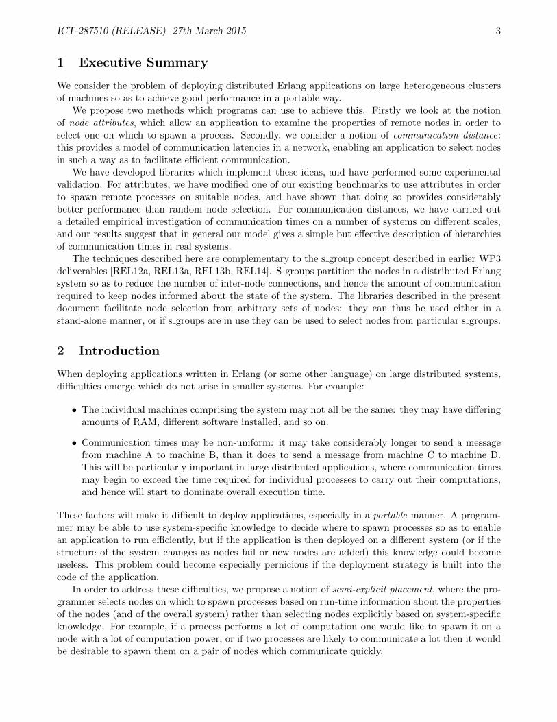
To study the hierarchical structure of our results we use a technique known as hierarchical agglomerativeclustering ([ELLS11, Chapter 4], [KR90]). This collects data points into clusters according to how closetogether they are. Furthermore, the clusters are arranged hierarchically, with small clusters groupedtogether to form larger ones, and so on.

The basic technique is as follows:

• Start off by placing every point in a cluster of its own.

• Look for the two clusters which are closest together and merge them to form a large cluster.

• Repeat the previous step until we have only a single cluster.

This process is illustrated in Figure 6.A question arises here: we know the distance between two points (that’s our basic data), but how

do we measure the distance between two clusters? Various methods can be used. For example, giventwo clusters A and B, any of the following could be used:

d(A,B) = max{d(a, b) : a ∈ A, b ∈ B}d(A,B) = mean{d(a, b) : a ∈ A, b ∈ B}d(A,B) = min{d(a, b) : a ∈ A, b ∈ B}

All of these methods (and others) are used in the clustering literature (see [ELLS11] or [KR90], forexample), and all are useful in different situations. We have chosen the first method, which is knownas the complete linkage method: d(A,B) = max{d(a, b) : a ∈ A, b ∈ B}. In terms of communicationtimes, this tells us what the worst-case communication time between a node in A and a node in B is;this is reasonable from our point of view because we wish to have upper bounds on communicationtime.

The hierarchical structure of clusters and subclusters can be displayed in a type of diagram called adendrogram. This is a tree which has one node for each cluster, with the children of a cluster being itssubclusters. Figure 7 shows the dendrogram corresponding to Figure 6. The dendrogram was obtainedusing the hclust command in the R system for statistical analysis and visualisation [R C14], usingdistances between points measured directly from Figure 6. The dendrogram describes the hierarchicalnested structure seen at the end of Figure 6, with the height of the internal nodes of the dendrogramreflecting the distances between the corresponding subclusters.


a b

c

d

e

f

g

h i

a b

c

d

e

f

g

h i

a b

c

d

e

f

g

h i

a b

c

d

e

f

g

h i

a b

c

d

e

f

g

h i

a b

c

d

e

f

g

h i

a b

c

d

e

f

g

h i

a b

c

d

e

f

g

h i

a b

c

d

e

f

g

h i

Figure 6: Hierarchical clustering


f

g

h i

e

c d

a b

050

100

150

Hei

ght

Figure 7: Corresponding dendrogram

4.4 Measurements

We ran our distance-measuring Erlang application on several systems. Firstly we used it on a smallscale to look at inter-processor communication times within a multicore system, then we used it on alarger scale to look at inter-node communication times on two sizeable networks.

Our technique was to run Erlang VMs on each of the components of the system (processing unitswithin a single SMP machine, individual physical machines within a network), and measure the averagetime taken to send several messages back and forth between each pair of VMs. More precisely, our basicunit of measurement was the time taken to send 100 messages back and forth: we chose this numberbecause the time taken for a single message can be close to the one-microsecond resolution of Erlang’stimer:tc function, so it’s difficult to get precise times for single messages.

For each pair of VMs, we actually measured the mean time over 100 such 100-message batches, andused that as our final data. This was an attempt to make sure that our figures were representative:with a smaller number of datapoints, there was a danger that (for example) one of the VMs might havebeen swapped out by the operating system when the messages arrived, adding an unusual delay. Bysending 100 batches we hoped to mitigate such effects.

We also tried two different strategies. In the first, we ran a single process on VM number 1 whichbroadcast messages to all other VMs in parallel; once this had finished, we ran a similar process onVM number 2, and then on VM number 3, and so on. In our second strategy, we ran such processeson all VMs concurrently, so that all pairs of VMs were communicating simultaneously. We found thatthis gave more interesting results, because high traffic densities made irregularities in communicationtimes more apparent.

It should be pointed out that running multiple VMs on the same physical machine is not obviouslya sensible thing to do: within a single VM, inter-process messages are transmitted directly within theVM, by copying data between VM data-structures. This is something like 40 times faster than TCP/IPcommunication between two VMs on the same physical machine, and hence having more than one VM


would appear to lead to inefficiency. However, this is not necessarily the case. If a VM doesn’t requiretoo many resources, then pinning it to some subset of the cores (on a single socket, for example) mightenable it to benefit from the same locality effects that we have seen above, and hence to operate moreefficiently than if it is using all of the cores. Whether or not this is desirable would depend on theapplication being run.

4.4.1 Eight core machine

Firstly, we ran our experiment on an 8-core SMP machine, with one Erlang VM pinned to each core.The CPU was an Intel Xeon E5504, whose structure is shown in Figure 8. A dendrogram obtainedfrom our measurements is shown in Figure 9.

Figure 8: Eight-core machine (two sockets like this)

4 5 6 7

0 1

2 3

6.8

7.0

7.2

7.4

7.6

7.8

Hei

ght

Figure 9: Dendrogram for eight-core machine

The structure of the dendrogram (and hence the communication times from which it was derived)


reflects the NUMA structure of the machine very closely. Erlang uses TCP/IP for inter-VM communi-cations, and when the VMs are on the same host, this will take place via the Application layer of theTCP/IP protocol [Bra89], where messages are transmitted within memory by the OS. This means thatthere will be very little overhead, so communication times are strongly affected by the cache structureof the machine.

4.4.2 Forty-eight core machine

We also ran our experiment on a machine with 48 AMD Opteron 6348 processors. The structure of themachine is shown in Figure 10 and a dendrogram of our results in Figure 11. Once again, we see thatthe communication times have a strongly hierarchical structure corresponding to the NUMA structureof the physical machine.

Figure 10: Forty-eight-core machine (four sockets like this)


42 43 44 45 46 47 36 3738 39 40 41 28 29 24 25 30 31 20 21 32 33

18 1922 23 10 11 6 7 34 35 2 3 8 9 4 5

16 170 1

26 27 12 1314 15

45

67

89

10

Hei

ght

Figure 11: Dendrogram for forty-eight-core machine


4.4.3 Departmental network

We also ran our tests on some machines in a departmental network at Heriot-Watt University. We used39 machines, including a 34-node Beowulf cluster. The results are shown in Figure 12.

bwlf15

bwlf18

bwlf05

bwlf34

bwlf03

bwlf14

bwlf30

bwlf24

bwlf29

bwlf02

bwlf09

bwlf22

bwlf23

bwlf28

bwlf17

bwlf26

bwlf04

bwlf07

bwlf06

bwlf12

bwlf08

bwlf16

bwlf32

bwlf25

bwlf27

bwlf31

bwlf01

bwlf11

bwlf13

bwlf20

bwlf33

bwlf10

bwlf19

bwlf21

amaterasu

persephone

oberon

cantor

osiris

10 15 20 25 30

Height

Figure 12: Dendrogram for departmental network

The results are less clear-cut here. The dendrogram picks out the Beowulf cluster, but it’s not obviouswhat is happening with the other machines.


4.4.4 EDF’s Athos cluster

Our final test-case was EDF’s Athos cluster. Athos has 776 compute nodes, called atcn001–atcn776:each of these has 64GB of RAM and 24 Intel Xeon E5-2697 v2 processors. In the RELEASE project wehave a simultaneous access to up to 256 nodes (6144 cores) for up to 8 hours at a time. Users interactwith the cluster via a front-end node and initially have no access to any of the compute nodes. Access tothe compute nodes is obtained via the SLURM workload manager (see http://slurm.schedmd.com/),either interactively or via a batch script which specifies how many nodes are required, and for how long.Jobs wait in a queue until sufficient resources are available, and then SLURM allocates a number ofcompute nodes, which then become accessible (via ssh, for example). The user has exclusive access tothese machines, and no-one else’s code will be running at the same time. Fragmentation issues meanthat jobs are not usually allocated a single contiguous block of machines, but rather some subset scat-tered through the cluster: for example atcn[127-144,163-180,217-288,487-504,537-648,667-684].These will be interspersed with machines allocated to other users: see Figure 13, which shows a screen-shot from SLURM’s smap command at a time when the Athos cluster was fairly busy.

Figure 13: SLURM allocation

The area at the top contains a string of characters, one for each machine in the cluster (wrapping roundat the end of lines in the usual way). Dots represent unallocated machines, and coloured alphanumericcharacters correspond to the jobs running on the machines; information about some of the jobs is shownin the lower part of the figure, with usernames and job names obscured. Note for example how the jobslabelled S and V are fragmented.

Users can request specific (and perhaps contiguous) node allocations, but it may take a long timebefore the desired nodes are all free at once, leading to a very long wait in the SLURM queue.

Athos was somewhat problematic. As we shall see shortly, communication times were highly non-uniform. We hypothesise that Athos communication takes place via a hierarchy of routers, but theprecise structure of the cluster is not publicly available. Furthermore, SLURM tends to allocate a


different set of nodes to each job, so it is difficult to get repeatable results.The next few figures illustrate the complicated communication structure that we have observed.

Figure 14 shows a dendrogram for communication times in a 256-node SLURM allocation on theAthos cluster (the names of the machines are omitted because they are illegibly small). We can seenine or ten distinct subclusters with fast intra-cluster communication, but with substantially slowercommunication between the subclusters. However, it’s difficult to determine exactly what’s going ondue to the denseness of the diagram.

..

..

..............................

.

..

..

..

...............................

..

..

..

..............................

..

.

..

...

............................

..

..

........................

.

..

..

..

.

.

.

................

..................

........................................

0 200 400 600 800

Height

Figure 14: Dendrogram for Athos cluster

In an effort to make the data more comprehensible, Figure 15 show four views from a three-dimensional plot of the communication times. The x- and y- axes show the source and target nodes(ie, the nodes which are sending and receiving messages, respectively), and there is one point for each


pair of machines, whose z-coordinate represents the mean communication time observed between thosemachines. These points are coloured according to the source machine, in an attempt to make theperspective views easier to interpret. It is clear that communication times are highly quantised: forsome pairs of machines, the mean time taken to exchange 100 messages is on the order of 25ms, whereasfor others, it is over 800ms. This is a 32-fold difference.

Figure 15: Athos communication times


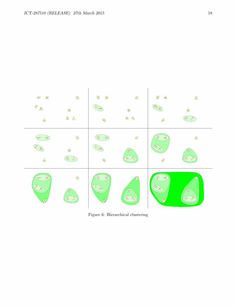
Another plot of these times is shown in Figure 16. This is a heatmap, which is rather like an over-head view of Figure 15, with points coloured according to communication times: red represents fastcommunication, yellow and white slower communication.

50 100 150 200 250

5010

015

020

025

0

Source

Targ

et

Figure 16: Heatmap for Athos communication times

Recall that SLURM usually allocates nodes in fragmented blocks: in this case, the allocation wasatcn[019-036,073-126,145-216,451-468,487-522,541-594,750-753]. It is tempting to suspectthat the block structure seen in Figure 16 corresponds to the blocks within the allocation, but thisis not quite the case. In Figure 17 we have added dotted lines to show where the breaks in theallocation occur. We see that the breaks in the allocation correspond to some of the discontinuities inthe communication times, but not all of them. Furthermore, there are areas where nodes in differentblocks of the allocation communicate very quickly, for example the small red block at approximately(250,70).


50 100 150 200 250

5010

015

020

025

0

Source

Targ

et

Figure 17: Heatmap for Athos communication times (2)

There is certainly some dependence on the SLURM allocation. Plots obtained with different allocationsdiffer in detail, but are qualitatively very similar to the ones above.

Remark. It is worth noting that communication times vary with the amount of network traffic.We also ran our test program with a different strategy, where one machine at a time would exchangemessages with all of the others, then the next machine would do the same thing, and so on; this involvesmuch less network traffic. Figure 18 shows a plot of some data obtained with this strategy during thesame SLURM job as above. The distribution is clearly much smoother, and all communication betweendifferent machines takes between about 50ms and 60ms for 100 exchanges. This contrasts strongly withthe situation in Figure 15, where the mean communication time is much slower (585ms, as opposedto 58ms); Oddly, some of the communication is actually faster in Figure 15, where about 10% of theexchanges take between 20ms and 40ms.


Figure 18: Athos communication times (low network traffic)

Discussion. The earlier figures show that Athos does have a very hierarchical communication struc-ture (at least when there is a lot of network traffic), but we have been unable to determine exactlywhat that structure is. Information about the construction of the network is not available to us, but wehypothesise that there is some tree-shaped hierarchy of routers. When there’s a lot of network traffic(as there was in these experiments, where all nodes were talking to all others simultaneously) this wouldmean that some messages would have to travel up and back down through several layers of routers,and some of the routers would become congested. There appears to be an extra complication thatnode names don’t correspond cleanly to the hierarchical structure of the network; this would explainthe off-diagonal areas of fast communication in the heatmaps above. The situation is made even worseby the fact that we can’t observe the whole network at once: we can only look through the 256-nodewindows supplied by SLURM.

This is somewhat problematic. There are clearly different levels of communication times, and thisis exactly what our model is supposed to deal with. Our planned strategy is to look at the structure ofthe network, use it to write down a tree, and then use the ultrametric structure on the tree to aid inprocess placement; unfortunately, in this case we aren’t able to write down the required tree becausethe structure of the network is difficult to observe.

4.5 Determining cluster structure automatically

We have a plan to deal with these difficulties. At the start of a SLURM job on Athos, we could run ourtest program to gather timing data, then perform cluster analysis to obtain a dendrogram. This couldthen be used as input to our metric space method, which could then be used for process placement.Standard cluster analysis is not quite suitable for this, because it always creates binary trees: lookingagain at the Athos dendrogram in Figure 14, it can be seen that the clusters at the bottom of thediagram consist of cascades of binary branches. Clearly, single clusters with multiple elements are whatis required.

We have implemented an algorithm which does this. This involves a slight modification of thestandard clustering algorithm described at the beginning of §4.3.2. Our algorithm involves a user-defined threshold α ≥ 1, and proceeds as follows:


• Start off by placing every point in a cluster of its own.

• Look for the two clusters which are closest together and merge them to form a larger cluster K.

• Let δ = diam(K) = max{d(a, b) : a, b ∈ K}.

• Expand K by adding points x with d(x,K) ≤ αδ. This forms a cluster of roughly equidistantpoints, the degree of roughness being determined by α.

• Repeat this process until we have only a single cluster. At each step, δ should be equal to thediameter of the current version of K.

This produces a non-binary dendrogram of the type we require. This is a fairly simple extension of thestandard clustering algorithm, and one would expect that it would be well-known; however, we havenot yet been able to find a reference in the clustering literature (but see [BTH11], where considerablymore sophisticated methods are used to tackle problems of this type).

We have applied this method with various values of α to the Athos data in the previous section,and the results are shown in Figures 19–25.

Unfortunately, R cannot render non-binary dendrograms of the type we have constructed here, sowe have had to resort to yet another visualisation, this time obtained by getting our clustering programto produce output for the dot tool of the Graphviz package [GN00]. Elliptical nodes represent clustersat the lowest levels, and contain the numbers of the relevant machines, together with the size of thecluster and its diameter (ie, the maximum communication time between two nodes in the cluster).Square nodes indicate higher level clusters (themselves formed from smaller clusters) and contain thecluster’s diameter.

When α = 1.0 we are essentially reproducing the standard binary clustering algorithm, and weobtain a dendrogram with one node for each machine (this corresponds to Figure 14).

880ms

45ms 842ms

54 44ms

28 40ms

32 37ms

[25,50]2 nodes37ms

36ms

37 32ms

38 29ms

29ms 28ms

30[43,53]2 nodes27ms

28ms 28ms

[33,51]2 nodes27ms

28ms

[41,44]2 nodes26ms

27ms

[20,23]2 nodes25ms

27ms

[29,35]2 nodes26ms

27ms

40 26ms

24[27,36]2 nodes25ms

28ms 28ms

[22,34]2 nodes26ms

27ms

48[31,46]2 nodes26ms

28ms[49,52]2 nodes26ms

26 27ms

[21,39]2 nodes27ms

27ms

[19,47]2 nodes26ms

[42,45]2 nodes26ms

69ms 835ms

222 44ms

216 38ms

206 33ms

220 29ms

225 27ms

27ms 27ms

205 26ms

[213,215]2 nodes26ms

26ms

221[202,228]2 nodes26ms

27ms 27ms

[199,224]2 nodes26ms

27ms

218 27ms

26ms 26ms

229[201,230]2 nodes26ms

[203,223]2 nodes26ms

26ms

25ms[231,233]2 nodes25ms

214[207,217]2 nodes25ms

26ms 27ms

26ms 26ms

210[204,208]2 nodes25ms

232[200,211]2 nodes25ms

26ms[226,234]2 nodes26ms

212 26ms

227[209,219]2 nodes25ms

74ms 755ms

81 66ms

103 44ms

82 37ms

77 33ms

96 29ms

108 28ms

28ms 28ms

104 27ms

[78,99]2 nodes27ms

[83,92]2 nodes27ms

27ms 27ms

98[91,101]2 nodes27ms

27ms 27ms

[84,87]2 nodes26ms

[95,107]2 nodes26ms

26ms 27ms

97[74,80]2 nodes26ms

27ms 27ms

79 27ms

26ms[102,106]2 nodes25ms

75[73,90]2 nodes25ms

27ms 27ms

88[89,105]2 nodes26ms

[86,93]2 nodes26ms

27ms

[76,100]2 nodes25ms

[85,94]2 nodes26ms

74ms 546ms

143 67ms

136 47ms

144 47ms

132 44ms

137 41ms

138 39ms

131 38ms

112 33ms

133 28ms

142 27ms

110 27ms

27ms 27ms

134 27ms

130[111,118]2 nodes26ms

27ms 27ms

26ms 27ms

120[127,139]2 nodes26ms

121 27ms

27ms 26ms

113 26ms

[114,116]2 nodes26ms

26ms

141[117,126]2 nodes26ms

123 26ms

129[115,122]2 nodes26ms

26ms 26ms

125 26ms

135[109,124]2 nodes26ms

140[119,128]2 nodes26ms

42ms 350ms

56 38ms

6 36ms

1 32ms

57 28ms

26ms 27ms

63 25ms

5[3,11]

2 nodes25ms

27ms 27ms

18[7,10]

2 nodes25ms

27ms 27ms

26ms 26ms

4[9,12]

2 nodes26ms

[2,15]2 nodes25ms

[62,66]2 nodes25ms

26ms 27ms

[13,16]2 nodes25ms

[59,65]2 nodes25ms

[17,55]2 nodes26ms

27ms

26ms 25ms

8[14,60]2 nodes26ms

61[58,64]2 nodes24ms

85ms 218ms

145 58ms

196 39ms

153 33ms

160 28ms

195 26ms

[147,156]2 nodes25ms

25ms

25ms[159,198]2 nodes25ms

149 25ms

[150,197]2 nodes25ms

25ms

[146,194]2 nodes24ms

25ms

24ms 25ms

161[155,158]2 nodes24ms

24ms[151,154]2 nodes24ms

148 24ms

157 23ms

193[152,162]2 nodes23ms

34ms 169ms

179 25ms

170 25ms

165 25ms

25ms 25ms

171 24ms

169 24ms

172[168,173]2 nodes23ms

24ms 25ms

164 24ms

175 24ms

176 24ms

[163,167]2 nodes24ms

[166,178]2 nodes24ms

174[177,180]2 nodes24ms

33ms 60ms

245 26ms

241 25ms

239 24ms

244 24ms

248 24ms

242 24ms

24ms 24ms

251 24ms

240 24ms

237[238,250]2 nodes23ms

24ms[243,246]2 nodes24ms

235 23ms

252 23ms

247[236,249]2 nodes23ms

26ms 28ms

191 25ms

183 25ms

182 25ms

192 25ms

24ms 24ms

189[186,190]2 nodes24ms

24ms[187-188]2 nodes24ms

184[181,185]2 nodes24ms

26ms 25ms

70 25ms

25ms[68,72]2 nodes24ms

67[69,71]2 nodes24ms

256 24ms

254[253,255]2 nodes23ms

Figure 19: α = 1.0


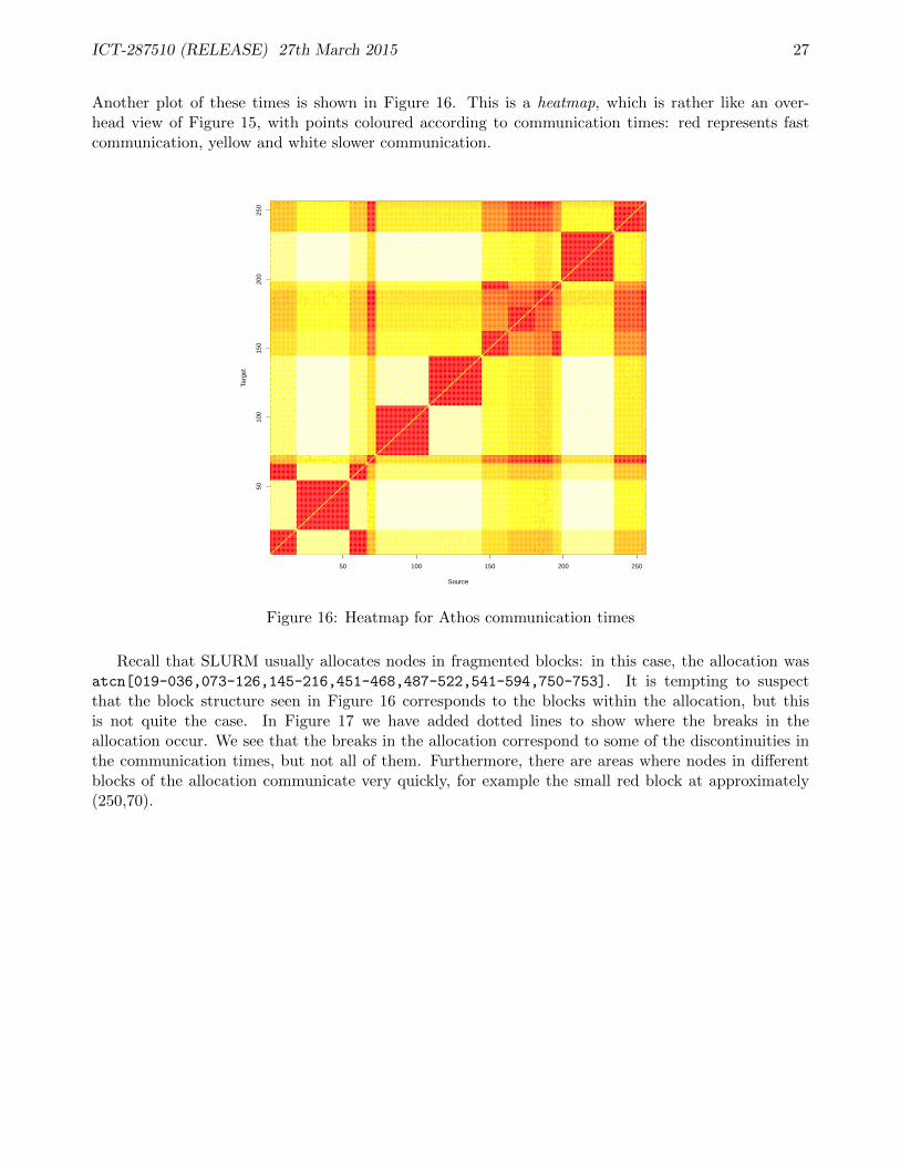
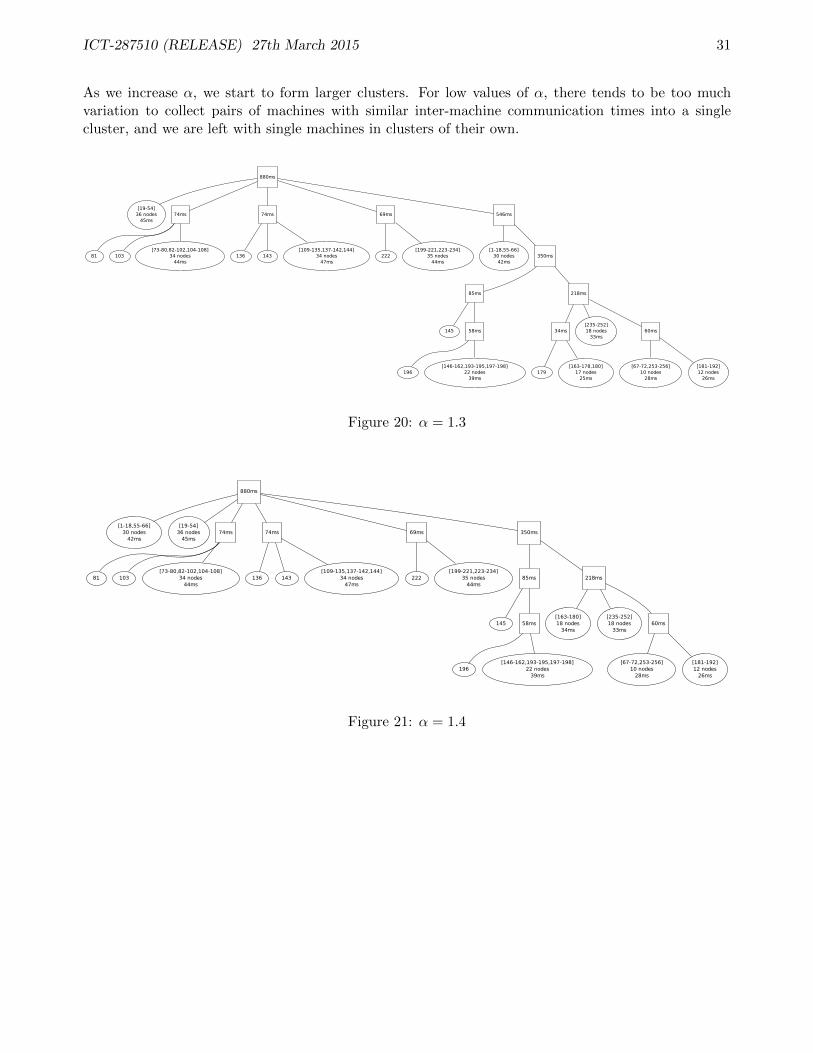
As we increase α, we start to form larger clusters. For low values of α, there tends to be too muchvariation to collect pairs of machines with similar inter-machine communication times into a singlecluster, and we are left with single machines in clusters of their own.

880ms

[19-54]36 nodes

45ms74ms 74ms 69ms 546ms

81 103[73-80,82-102,104-108]

34 nodes44ms

136 143[109-135,137-142,144]

34 nodes47ms

222[199-221,223-234]

35 nodes44ms

[1-18,55-66]30 nodes

42ms350ms

85ms 218ms

145 58ms

196[146-162,193-195,197-198]

22 nodes39ms

34ms[235-252]18 nodes

33ms60ms

179[163-178,180]

17 nodes25ms

[67-72,253-256]10 nodes

28ms

[181-192]12 nodes

26ms

Figure 20: α = 1.3

880ms

[1-18,55-66]30 nodes

42ms

[19-54]36 nodes

45ms74ms 74ms 69ms 350ms

81 103[73-80,82-102,104-108]

34 nodes44ms

136 143[109-135,137-142,144]

34 nodes47ms

222[199-221,223-234]

35 nodes44ms

85ms 218ms

145 58ms

196[146-162,193-195,197-198]

22 nodes39ms

[163-180]18 nodes

34ms

[235-252]18 nodes

33ms60ms

[67-72,253-256]10 nodes

28ms

[181-192]12 nodes

26ms

Figure 21: α = 1.4


880ms

[1-18,55-66]30 nodes

42ms

[19-54]36 nodes

45ms74ms

[109-144]36 nodes

74ms69ms 350ms

81 103[73-80,82-102,104-108]

34 nodes44ms

222[199-221,223-234]

35 nodes44ms

[145-162,193-198]24 nodes

85ms218ms

[163-180]18 nodes

34ms

[235-252]18 nodes

33ms60ms

[67-72,253-256]10 nodes

28ms

[181-192]12 nodes

26ms

Figure 22: α = 1.5

When we reach α = 1.6, we obtain what may be thought of as the “real” cluster structure, with 10small clusters corresponding to those seen in Figure 14. Increasing α still further, we start to losethe higher-level subclusters, until at α = 2.5 we only have the low-level clusters, and have lost all ofthe higher-level structure. For even bigger values of α, the algorithm becomes completely unable todistinguish between the individual machines, and we end up with a graph consisting of a single largecluster (Figure 26).

880ms

[1-18,55-66]30 nodes

42ms

[19-54]36 nodes

45ms

[73-108]36 nodes

74ms

[109-144]36 nodes

74ms

[145-162,193-198]24 nodes

85ms

[199-234]36 nodes

69ms218ms

[163-180]18 nodes

34ms

[235-252]18 nodes

33ms60ms

[67-72,253-256]10 nodes

28ms

[181-192]12 nodes

26ms

Figure 23: α = 1.6


880ms

[1-18,55-66]30 nodes

42ms

[19-54]36 nodes

45ms

[73-108]36 nodes

74ms

[109-144]36 nodes

74ms

[145-162,193-198]24 nodes

85ms

[163-180]18 nodes

34ms

[199-234]36 nodes

69ms

[235-252]18 nodes

33ms60ms

[67-72,253-256]10 nodes

28ms

[181-192]12 nodes

26ms

Figure 24: α = 2.0

880ms

[1-18,55-66]30 nodes

42ms

[19-54]36 nodes

45ms

[67-72,181-192,253-256]22 nodes

60ms

[73-108]36 nodes

74ms

[109-144]36 nodes

74ms

[145-162,193-198]24 nodes

85ms

[163-180]18 nodes

34ms

[199-234]36 nodes

69ms

[235-252]18 nodes

33ms

Figure 25: α = 2.5

[1-256]256 nodes

880ms

Figure 26: α = 3.0

This algorithm is still not perfect: we have to make a subjective choice of a value of α which gives usa satisfactory structure; furthermore, a single value of α may not be appropriate at all scales. There isquite a lot of variation in communication times in the small clusters, so we need a largish value of α inorder to detect the clusters. However, variations at larger scales are more subtle, so there is a danger oflosing higher-level hierarchical structures with large values of α, as in Figures 24 and 25. The Bayesianmethods of [BTH11] might be helpful here, but we do not have an implementation of this.

Nonetheless, our algorithm (with, say, α ∈ [1.5, 2.0]) is able to detect the low-level clusters withfast inter-machine communication times. Furthermore, our implementation has an alternative outputformat (in the form of an Erlang term) which is suitable for use by our communication-distance library.

4.6 Experimental evaluation

We had hoped to perform experiments to test the validity of our methods, but lack of time has preventedus from doing this. However, we will describe the experiment we had planned to carry out.

Consider the multi-level ACO application (ML-ACO) again (see §3.4.1). Recall that here we havea tree of submaster nodes collecting results from colonies. Each submaster calculates the best resultfrom the subtree which it is managing, then passes this up the hierarchy, where another submasterwill compare it with results from other subtrees. Eventually all of these pass up the tree to the master


node, which selects the globally-best solution. This is then propagated back down the tree to the colonynodes.

Now different pairs of nodes can have different communication times, as we have seen above. If wehave a descending path through the tree where several submasters are a long way from their childrenin communication terms, then a communication delay will be incurred at several points as messagestravel up and down the tree, leading to a slowdown in the overall execution times: see Figure 27, wherered edges represent slow communication.

M

S S S

S S S

C C C C C C C C C

Figure 27: Bad placement

Clearly we wish to avoid this situation. It may not be possible to avoid some slow communication,but we should try to avoid this happening more than once in each path through the tree: see Fig-ure 28. With sufficient knowledge of communication distances, it should be possible to arrange processplacement so as to avoid long chains of slow communication.

M

S S S

S S S

C C C C C C C C C

Figure 28: Good placement

Having implemented this, our plan was to run a SLURM job on Athos which would run ourcommunication-time-measuring program, then feed the output to our clustering algorithm to gener-ate a description of the subnetwork allocated by SLURM, then use this as input to our distance-awareML-ACO program. The first two steps here are only required because we do not have a static descrip-tion of the Athos network. We could also try this on a system of whose structure we do have a staticdescription, but we have as yet been unable to find a suitable candidate.

Postscript. We have in fact succeeded in getting some preliminary results from this experiment onthe Athos cluster. Unfortunately our results are both incomplete and inconclusive, and we will notreport the details here. We hope to continue with this work after the end of the project.


5 Discussion

We have described two concepts which we believe will be useful for producing performance-portableErlang applications: node attributes and communication distances. Both of these can be used to helpin making a sensible choice of nodes to spawn processes on, and we have described libraries which makeit possible for applications to use these concepts without requiring system-specific information to beembedded in their source code.

5.1 Practical issues

The libraries for attributes and communication distances described above are prototypes, and ourexperience so far suggests several factors which it would be helpful to modify in libraries intended forgeneral use.

5.1.1 Concrete and abstract bounds

In practice it may be somewhat difficult to know what concrete bounds to use to make a choice ofnodes. For instance, at a particular time there may be no nodes satisfying {loadavg5, lt, 0.1} butseveral satisfying {loadavg5, lt, 0.3}. For practical use it might be worth having predicates like{loadavg5, low} and {cpu_speed, high} which would examine an entire list of candidate nodes andselect the ones whose attributes are relatively “good” in comparison with the majority.

Similarly, programmers should not have to know about explicit distances. Note that distances varywith the depth of a network hierarchy: in a shallow network, the nearest node to a specified nodemight be at a distance of 1

4 , whereas in a deeper network it could be at a distance of 132 . In order

to avoid this, we should provide the programmer with some abstractions such as {very_near, near,

far, very_far, anywhere}.

5.1.2 Conflicting constraints

Another issue is that a programmer may supply conflicting constraints. For example, one might askfor a node which has a large number of cores and has a particular library installed, but it may not bepossible to satisfy both requirements at once. One could overcome this to some extent by (for example)giving priority to the earlier constraints in a list. For debugging purposes, it could be useful to includea mode in which such conflicts are reported at runtime.

5.1.3 Avoiding clashes when spawning processes

There may be some danger in using attributes to select nodes. If a large number of processes arespawning other processes, there is a possibility that many of them may select the same node, and thenperformance will suffer. This could be mitigated to some extent by making a random choice from a listof suitable candidates, but there could be problems if there is a unique node which has some particularlydesirable properties. At some point it may be necessary to spawn processes on a suboptimal node, butit’s not entirely clear how to do this in a portable manner.

5.1.4 Fault-tolerance

Our attribute scheme is highly-fault tolerant as long as no applications dynamically modify the at-tributes of a node. Suppose that only static and built-in attributes are used: in the event of theattribute server crashing, it can simply be restarted and all of the node attributes will be restored;similarly, if an application process crashes then it can be restarted and the node attributes will be thesame as they were before the crash. However, if an application modifies the attributes (for example, to


register the fact that it’s running on the node), then if the attribute server crashes, this information willbe lost; if the application crashes then the attribute server could be left with stale attributes belongingto a defunct process. This suggests that allowing applications to modify node attributes may be a badidea.

5.1.5 Dynamic changes to network structure

Our current distance scheme depends on a static description of the network structure. In a long-running system, it is likely that nodes will leave the system, or that new ones may join. We have somepreliminary ideas as to how to deal with this problem, but this will require further work.

6 Conclusions

Our experimental validation has been less comprehensive than we would have liked, but we believe thatwe have demonstrated that attributes and communication distances can be useful in practice. We haveshown that the use of attributes can have substantial performance benefits in a realistic application.Ideally we would like to validate our methods by applying them to a large real-world Erlang applicationrunning on a number of different distributed systems.

Despite the fact that we haven’t validated the distance methods in the context of running Erlangapplications, we believe that our work shows the the ideas will be useful in distributed systems withnon-uniform communication times. Our examination of the Athos system and SMP machines showsthat hierarchical communication structures do appear in practice, and that communication times canvary significantly according to the relative positions of nodes in the hierarchy. Our abstract modelclearly captures this type of structure, and hence should be well suited for deploying processes in sucha way as to take account of communication times. The benefit of the model is that it captures thehierarchical structure while disregarding precise details of timing, and can be constructed from a fairlyhigh-level view of the system (assuming such a view is available).

We intend to carry on investigating these ideas beyond the end of the RELEASE project. Commu-nication distances in particular are a promising idea, and may have general applicability in the area ofdistributed systems.

A Appendix: Querying attributes in a real system

This section contains a demonstration of the attr library in action, with the aim of giving the readera feel for its behaviour.

We ran Erlang VMs on a number of machines at Heriot-Watt University. The machines werecalled bwlf01, bwlf02, bwlf03, bwlf04, bwlf10, bwlf15, bwlf16, bwlf17, bwlf18, bwlf19, bwlf20,bwlf32, bwlf32, bwlf33, bwlf34, amaterasu, osiris, persephone, cantor, oberon, and jove (withthe exception of jove, these are the same machines considered in §4.4.3). The bwlfNN machines arepart of a Beowulf cluster, and the others are non-Beowulf machines connected to the departmentalnetwork.

There was one Erlang VM called vm1 on all of the machines except for bwlf10, which had threeVMs pinned to subsets of its 8 processors (vm1 on core 0, vm2 on cores 1 and 2, and vm3 on cores 3–8).

There’s an extract from an Erlang session querying the attributes of these VMs below. Some lineshave been omitted because of typing errors or uninteresting results. The VMs were started without aconfiguration file, so all of the queries below use only built-in attributes.


(m@localhost)1> Nodes = nodes:nodes().

% This is just a function which returns a fixed list, to make it

% easy to get the node names into the Erlang shell.

[vm1@bwlf01,vm1@bwlf02,vm1@bwlf03,vm1@bwlf04,vm1@bwlf15,

vm1@bwlf16,vm1@bwlf17,vm1@bwlf18,vm1@bwlf19,vm1@bwlf20,

vm1@bwlf32,vm1@bwlf32,vm1@bwlf33,vm1@bwlf34,vm1@amaterasu,

vm1@osiris,vm1@persephone,vm1@cantor,vm1@oberon,

vm1@localhost,vm1@bwlf10,vm2@bwlf10,vm3@bwlf10]

...

(m@localhost)4> attr:request_attrs(Nodes, [cpu_speed,mem_free]).

[{vm1@bwlf01,[{cpu_speed,1596.0},{mem_free,6845956}]},

{vm1@bwlf02,[{cpu_speed,1596.0},{mem_free,9690156}]},









{vm1@bwlf33,[{cpu_speed,1998.0},{mem_free,13948024}]}, % bwlf33 and bwlf34 are


{vm1@bwlf34,[{cpu_speed,1998.0},{mem_free,9832688}]}, % faster than the others

{vm1@osiris,[{cpu_speed,2666.0},{mem_free,217452}]},


{vm1@amaterasu,[{cpu_speed,1.6e3},{mem_free,13878268}]},

{vm1@persephone,[{cpu_speed,1998.0},{mem_free,754432}]},

{vm1@cantor,[{cpu_speed,2.8e3},{mem_free,435815476}]},

{vm1@oberon,[{cpu_speed,1.2e3},{mem_free,25687204}]},

{vm1@localhost,[{cpu_speed,1.6e3},{mem_free,8517844}]},



{vm3@bwlf10,[{cpu_speed,1596.0},{mem_free,10481680}]}]

(m@localhost)5> attr:request_attrs(Nodes, [loadavg5, vm_num_processors]).

[{vm1@bwlf01,[{loadavg5,0.04},{vm_num_processors,8}]},

{vm1@bwlf02,[{loadavg5,0.0},{vm_num_processors,8}]},













{vm1@amaterasu,[{loadavg5,0.0},{vm_num_processors,8}]},

{vm1@osiris,[{loadavg5,7.93},{vm_num_processors,24}]},

{vm1@persephone,[{loadavg5,0.0},{vm_num_processors,2}]},

{vm1@cantor,[{loadavg5,5.05},{vm_num_processors,48}]},

{vm1@oberon,[{loadavg5,0.0},{vm_num_processors,6}]},

{vm1@localhost,[{loadavg5,0.27},{vm_num_processors,24}]},


{vm1@bwlf10,[{loadavg5,0.01},{vm_num_processors,1}]}, % The VMs on bwlf10 are

{vm2@bwlf10,[{loadavg5,0.01},{vm_num_processors,2}]}, % running on subsets of

{vm3@bwlf10,[{loadavg5,0.01},{vm_num_processors,5}]}] % the full set of cores.

...

(m@localhost)8> attr:choose_nodes(Nodes, [{vm_num_processors, lt, 8}]).

[vm1@persephone,vm1@oberon,vm1@bwlf10,vm2@bwlf10,vm3@bwlf10]

(m@localhost)9> attr:choose_nodes(Nodes, [{vm_num_processors, ge, 8},{loadavg5, lt, 1}]).



vm1@bwlf32,vm1@bwlf33,vm1@bwlf32,vm1@bwlf34,vm1@amaterasu,

vm1@localhost]

(m@localhost)10> attr:choose_nodes(Nodes, [{vm_num_processors, ge, 8},{loadavg5, lt, 0.5}]).



vm1@bwlf33,vm1@bwlf34,vm1@amaterasu,vm1@localhost]

(m@localhost)11> attr:choose_nodes(Nodes, [{vm_num_processors, ge, 8},{loadavg5, lt, 0.1}]).


vm1@bwlf33,vm1@amaterasu]

(m@localhost)12> attr:choose_nodes(Nodes, [{loadavg5, lt, 0.1}, {cpu_speed, gt, 2000}]).

[]

...

(m@localhost)14> attr:choose_nodes(Nodes, [{loadavg5, lt, 0.1}, {cpu_speed, gt, 1600}]).

[vm1@bwlf01,vm1@bwlf33,vm1@persephone]

(m@localhost)15> q().

ok

Change Log

Version Date Comments

0.1 11/03/2015 First Version Submitted to Internal Reviewer.

0.2 21/03/2015 Revised version based on comments from S. Thompson

0.3 23/03/2015 Final version submitted to the Commission Services

0.4 27/03/2015 Minor corrections

References

[Bou] Boundary. Folsom. https://github.com/boundary/folsom.

[Bra89] R. Braden. RFC 1122 Requirements for Internet Hosts - Communication Layers. InternetEngineering Task Force, October 1989.


[BTH11] C. Blundell, Y. W. Teh, and K. A. Heller. Discovering non-binary hierarchical structureswith Bayesian rose trees. In K. Mengersen, C. P. Robert, and M. Titterington, editors,Mixture Estimation and Applications. John Wiley & Sons, 2011.

[ELLS11] Brian Everitt, Sabine Landau, Morven Leese, and Daniel Stahl. Cluster analysis. Wiley, 5thedition, 2011.

[Feu] Feuerlabs. Exometer. https://github.com/Feuerlabs/exometer.

[GN00] Emden R. Gansner and Stephen C. North. An open graph visualization system and itsapplications to software engineering. SOFTWARE - PRACTICE AND EXPERIENCE,30(11):1203–1233, 2000. See www.graphviz.org.

[HS65] Edwin Hewitt and Karl Stromberg. Real and abstract analysis. A modern treatment of thetheory of functions of a real variable, volume 25 of Graduate Texts in Mathematics. Springer-Verlag, New York, 1965.

[KR90] L. Kaufman and P. J. Rousseeuw. Finding groups in data: an introduction to cluster analysis.John Wiley and Sons, New York, 1990.

[Kra44] Marc Krasner. Nombres Semi-Reels et Espaces Ultrametriques. Comptes Rendus del’Academie des Sciences, Tome II, 219:433–435, 1944.

[MST14] P. Maier, R. Stewart, and P.W. Trinder. Reliable scalable symbolic computation: Thedesign of SymGridPar2. Computer Languages, Systems & Structures, 40(1):19 – 35, 2014.Special issue on the Programming Languages track at the 28th ACM Symposium on AppliedComputing.

[R C14] R Core Team. R: A Language and Environment for Statistical Computing. R Foundationfor Statistical Computing, Vienna, Austria, 2014.

[REL12a] RELEASE Project. Deliverable D3.1: Scalable Reliable SD Erlang Design, June 2012.

[REL12b] RELEASE Project. Deliverable D4.3: Heterogeneous super-cluster infrastructure, December2012.

[REL13a] RELEASE Project. Deliverable D3.2: Scalable SD Erlang Computation Model, July 2013.

[REL13b] RELEASE Project. Deliverable D3.3: Scalable SD Erlang Reliability Model, September2013.

[REL13c] RELEASE Project. Deliverable D4.4: Capability-driven Deployment, May 2013.

[REL14] RELEASE Project. Deliverable D3.4: Scalable Reliable OTP Library Release, September2014.

[REL15a] RELEASE Project. Deliverable D4.5: Scalable Infrastructure Performance Evaluation re-port, February 2015.

[REL15b] RELEASE Project. Deliverable D5.4: Interactive SD Erlang Debugging, February 2015.

[REL15c] RELEASE Project. Deliverable D6.2. Scalability Case Studies: Scalable Sim-Diasca for theBlueGene, March 2015.

[Rud76] W. Rudin. Principles of Mathematical Analysis. International series in pure and appliedmathematics. McGraw-Hill, 1976.

d3.5 (wp3): sd erlang performance portability · pdf filesd erlang performance portability...

Documents