daniel gros - thinking ahead for europe economy in 2030_small_0.pdf · the global economy in 2030...
TRANSCRIPT

THE GLOBAL ECONOMY IN 2030
TRENDS AND STRATEGIES FOR EUROPE
DANIEL GROS AND
CINZIA ALCIDI
WITH CONTRIBUTIONS BY
ARNO BEHRENS, CEPS
STEVEN BLOCKMANS, CEPS
MATTHIAS BUSSE, CEPS
CHRISTIAN EGENHOFER, CEPS
LIONEL FONTAGNÉ, CIREM
ARNAUD FOUGEYROLLAS, SEURECO
GILLES KOLEDA, SEURECO
ILARIA MASELLI, CEPS
MARIA PRISCILA RAMOS, CIREM
CARLO SESSA, ISIS
PAUL ZAGAMÉ, SEURECO
CENTRE FOR EUROPEAN POLICY STUDIES (CEPS)
BRUSSELS

The Centre for European Policy Studies (CEPS) is an independent policy research institute in Brussels.
Its mission is to produce sound policy research leading to constructive solutions to the challenges facing
Europe. The views expressed in this book are entirely those of the authors and should not be attributed
to CEPS or any other institution with which they are associated or to the European Union.
This CEPS report was commissioned by the European Strategy and Policy Analysis System (ESPAS) – an
inter-institutional initiative of the European Commission, European Parliament, Council of the European
Union and the European External Action Service – with full respect for the intellectual independence
of CEPS. The preparation of the study was closely monitored by an ad-hoc inter-institutional Steering
Group (backed up by a dedicated Working Group), which guided the process and gave appropriate
feedback at regular intervals.
The findings of this report are the responsibility of the Centre for European Policy Studies (CEPS), and
do not necessarily express the opinions of the EU institutions or any of the other organisations with
which the contributors are affiliated.
© European Union, 2013.
Reproduction is authorised provided the source is acknowledged.
ISBN: 978-92-7929-721-2 / Catalogue number: NJ-30-13-614-EN-C
All rights reserved. No part of this publication may be reproduced, stored in a retrieval system or
transmitted in any form or by any means – electronic, mechanical, photocopying, recording or otherwise
– without the prior permission of the European Union.
Centre for European Policy Studies Place du Congrès 1, B-1000 Brussels
Tel: (32.2) 229.39.11 Fax: (32.2) 219.41.51 E-mail: [email protected] Internet: www.ceps.eu

Contents
Preface ............................................................................................................................................................................ i
Executive Summary ..................................................................................................................................................... 1
1. Introduction ......................................................................................................................................................... 5
Part I. Global Drivers of Growth ...................................................................................................... 8
2. Population and human capital ........................................................................................................................... 8
2.1 World population dynamics................................................................................................................... 8 2.2 Working age population and labour force ......................................................................................... 12 2.3 Quantity versus quality ......................................................................................................................... 13 2.4 Migration ................................................................................................................................................ 15 2.5 Urbanisation ........................................................................................................................................... 16
3. Capital and capital markets .............................................................................................................................. 19
3.1 Investment and capital accumulation as drivers of growth ............................................................ 19 3.2 The longer-term effects of high investment rates ............................................................................ 20 3.3 Savings versus investment.................................................................................................................... 21 3.4 Finance: A roadblock to recovery or a necessary ingredient of development? ........................... 22 3.5 Conclusions ............................................................................................................................................ 23
4. Globalisation ...................................................................................................................................................... 23
4.1 Trade ....................................................................................................................................................... 23 4.2 Global value-added chains: A revolution of trade patterns? .......................................................... 28 4.3 Investment flows ................................................................................................................................... 33 4.4 Longer-term trends in trade and financial globalisation ................................................................. 36 4.5 Conclusions ............................................................................................................................................ 38
5. Technology and innovation ............................................................................................................................. 39
5.1 Total factor productivity ...................................................................................................................... 39 5.2 Our predictions ...................................................................................................................................... 41 5.3 The impact of breakthrough technologies ........................................................................................ 43 5.4 Advanced technologies will not destroy jobs ................................................................................... 45
6. Natural resources: Energy and metals ........................................................................................................... 47
6.1 Energy ..................................................................................................................................................... 50 6.2 Metals ...................................................................................................................................................... 50 6.3 Water ....................................................................................................................................................... 51 6.4 The predictions of the model .............................................................................................................. 53 6.5 Shale gas and 2030 horizons for natural gas in Europe and the world ........................................ 54 6.6 Shale gas bonanza: Re-industrialisation or de-industrialisation? .................................................... 58 6.7 Energy resources: The sky (or rather the atmosphere) is the limit! .............................................. 60 6.8 Conclusions ............................................................................................................................................ 61
Part II. Economic Growth and Prosperity in 2030 ........................................................................ 62
7. The state of the global economy in 2030 ...................................................................................................... 62
7.1 Sensitivity analysis of the model ......................................................................................................... 66 7.2 Conclusions ............................................................................................................................................ 71
8. The impact of growth on affluence and poverty ......................................................................................... 73
9. The impact of growth on climate change ..................................................................................................... 75
9.1 The predictions of the model on climate change ............................................................................. 76 9.2 Conclusion .............................................................................................................................................. 77

Part III. The EU’s Transition towards 2030 .................................................................................. 79
10. The outcome of the NEMESIS model: Introduction................................................................................. 80
11. Europe as whole ................................................................................................................................................ 80
11.1 The first phase (2011-14): External balance the main driver for GDP ........................................ 81 11.2 The second phase (2014-18): The rebound in productivity ........................................................... 83 11.3 Third phase (2019-30): Losses in competitiveness .......................................................................... 83 11.4 The labour market ................................................................................................................................. 83 11.5 Sectoral employment ............................................................................................................................ 84 11.6 Public finances ....................................................................................................................................... 84
12. A more detailed approach ................................................................................................................................ 85
12.1 Characteristics of the three types of country .................................................................................... 85 12.2 The convergence ................................................................................................................................... 86 12.3 Slow and incomplete adjustments for unemployment and deleveraging ..................................... 88
13. The consequence of higher productivity gains ............................................................................................. 89
13.1 Calibration, allocation and implementation of the shock ............................................................... 89 13.2 Results for the whole of Europe ......................................................................................................... 90
14. Conclusions ........................................................................................................................................................ 90
Part IV. Policy Challenges and Game Changers for the EU .......................................................... 92
15. A smaller EU in the world economy ............................................................................................................. 92
16. Facing an ageing world ..................................................................................................................................... 96
16.1 Excess savings and productivity shortage in Europe ...................................................................... 96
17. The EU needs to focus its trade policy: TTIP versus the BRICs ............................................................. 97
18. Centrifugal forces in Europe ........................................................................................................................... 99
18.1 The global dimension of the re-nationalisation of financial markets in the euro area ............. 100
19. Climate change challenge ............................................................................................................................... 101
19.1 Adaptation and adaptation policy ..................................................................................................... 104
20. Demographic cooling down in the Euro-Mediterranean ......................................................................... 105
20.1 Enhancing cooperation with the Mediterranean region ............................................................... 106
21. Is the world economy becoming less democratic? .................................................................................... 107
22. A global game changer from China: Falling investment without rebalancing ...................................... 109
23. The economic emergence of sub-Saharan Africa ...................................................................................... 111
24. Hydraulic fracking: An unlikely game changer but a persistent policy challenge for Europe ............ 111
24.1 The Euro-Mediterranean energy challenge and opportunity ....................................................... 112
25. Conclusions ...................................................................................................................................................... 113
References ................................................................................................................................................................. 115
Annex A. MaGE and MIRAGE Central and Alternative Scenarios ............................................................... 125
Annex B. Capital Accumulation in China: Is overinvestment an issue? ........................................................ 132
Annex C. What to expect from TTIP or free trade with a BRIC nation: The example of India ............... 135
Annex D. The Results of the NEMESIS Model: Europe moving towards 2030 ........................................ 138
About the Partners in the Consortium ................................................................................................................. 187

List of Figures
Figure 1.1 Economic growth and prosperity: Inputs and impact ........................................................................ 6
Figure 2.1 Three scenarios for global population growth to 2050 (millions) ..................................................... 9
Figure 2.2 Fertility rates across continents (2012) ................................................................................................ 10
Figure 2.3 Population by continent and median age, projections for 2030 (mil.) ........................................... 10
Figure 2.4 Total support ratio (working age population per total dependents) of boom to bust ................. 11
Figure 2.5 Working age population – China and India ........................................................................................ 12
Figure 2.6 Changes in the global labour force (1980-2030) ................................................................................ 13
Figure 2.7 Paths of tertiary education expansion: MaGE Central scenario ..................................................... 15
Figure 2.8 Paths of tertiary education expansion: MaGE alternative scenario ................................................ 15
Figure 2.9 Income differentials in 2030: Average GDP per worker as % of EU average in selected regions ................................................................................................... 16
Figure 2.10 Level of urbanisation by region, 2011 and 2030 .............................................................................. 17
Figure 2.11 Urbanisation and income (change between 1985 and 2010) ......................................................... 18
Figure 3.1 Regional investment (% of GDP) ........................................................................................................ 19
Figure 3.2 Capital stocks ($ billion, 2005 dollars) ................................................................................................. 21
Figure 3.3 Capital intensity per capita (thousands of 2005 US dollars)............................................................. 21
Figure 4.1 Global exports as percentage of world GDP (1980-2014) .............................................................. 24
Figure 4.2 Comparison of exports in goods as a percentage of value-added in manufacturing and GDP, Japan, US and EU27 (1998-2011) ......................................................................................... 25
Figure 4.3 Comparison of exports in goods relative to value-added in manufacturing and GDP, China vs average of Japan, EU and US (1998-2011)............................................................................. 25
Figure 4.4 World growth of output and exports................................................................................................... 27
Figure 4.5 EU27 trading partners, 2012 vs 2030 .................................................................................................. 28
Figure 4.6 Domestic value-added in exports (1995-2009) .................................................................................. 31
Figure 4.7 Overall trade in goods and trade in manufacturing products (% of GDP) ................................... 33
Figure 4.8 Global current account transactions by type, 2011 ($ billion and % of total) .............................. 34
Figure 4.9 FDI intensity liabilities position, G7 vs BRICs .................................................................................. 35
Figure 4.10 Net FDI position in % of GDP, G7 and BRICs ............................................................................ 35
Figure 4.11 Trade and financial flows across economic development .............................................................. 37
Figure 5.1 Projections of total factor productivity (1980-2030) ......................................................................... 41
Figure 5.2 R&D spending scenarios, 2010-30 (current billion USD) ................................................................ 42
Figure 6.1 Real commodity prices in the very long run, 1900-2010 .................................................................. 48
Figure 6.2 Two scenarios for resource use ............................................................................................................ 49
Figure 6.3 Energy productivity (2005, USD per barrel) ...................................................................................... 53
Figure 6.4 Projections in oil price (2005, USD per barrel) .................................................................................. 54
Figure 6.5 Natural gas prices in the US, Europe and Japan, 1993-2012 ........................................................... 55
Figure 6.6 US production of natural gas ................................................................................................................ 57
Figure 6.7 Forecast of US net energy import ........................................................................................................ 57
Figure 6.8 Balance of trade in manufacturing and services against mineral fuels: US vs. EU ($ bn) ........... 59
Figure 7.1 GDP (at PPP) growth compared, 2010-30 ......................................................................................... 62
Figure 7.2 GDP growth PPP in 2030 (blue shading) and GDP per capita PPP ($ thousands) .................... 63
Figure 7.3 Regional GDP shares (current USD) .................................................................................................. 64
Figure 7.4 Regional GDP shares (at PPP) ............................................................................................................. 64
Figure 7.5 Shares in world GDP growth (PPP decade averages) ....................................................................... 65
Figure 7.6 Contribution to cumulated world GDP, by region (over decades, at constant prices) ............... 65
Figure 7.7 Contribution of individual variables to GDP levels .......................................................................... 69
Figure 7.8 Comparing growth under central and alternative scenarios ............................................................. 70

Figure 7.9 Global GDP share in 2030 (PPP) ........................................................................................................ 70
Figure 8.1 Middle class population by region, in 2012 and 2030 (millions) ..................................................... 74
Figure 8.2 Number of people in poverty (mn) ...................................................................................................... 75
Figure 11.1 Contribution of main components to the growth of GDP for EU27 (2010-30) ....................... 81
Figure 11.2 Labour productivity and real wage growth rates for the EU27 .................................................... 82
Figure 11.3 Public finance in the EU27 ................................................................................................................. 85
Figure 12.1 GDP per capita (2010) and average annual growth rate of GDP per capita (2010-30) ............ 86
Figure 12.2 GDP per capita in 2010 and average annual growth rate of GDP per capita (2010-20) .......... 87
Figure 12.3 GDP per capita in 2020 and average annual growth rate of GDP per capita (2020-30) .......... 87
Figure 12.4 Average annual growth rate of labour productivity and real wages (2010-30) ........................... 88
Figure 12.5 Public debt as percentage of GDP and unemployment rate in EU27 (2030)............................. 89
Figure 13.1 Deviation of EU27 employment and labour productivity from the reference scenario ........... 90
Figure 15.1 Bilateral trade flows and GDP share of the G3 power triangle .................................................... 93
Figure 15.2 IMF quotas based on economic fundamentals of 2013 and projected for 2030 ........................ 94
Figure 18.1 Quasi-risk-free securities in the euro area, 2012 (in billions of USD equivalent) .................... 101
Figure 20.1 Different demographic transitions: Youth ratio (15-29 year-olds as % of total population) . 106
Figure 21.1 Share in global GDP (in PPP) among Freedom House groups .................................................. 108
Figure 21.2 World average: Rule of law deficiency (%) ..................................................................................... 109
Figure A.A1 Energy price projections, 2004=1, 2004-35.................................................................................. 130
Figure A.D1 Labour productivity and real wage growth rates for the EU27, 2010-30 ................................ 140
Figure A.D2 GDP growth rate and contribution of main components to this growth for the EU27, 2010-30 ....................................................................................................................................................... 141
Figure A.D3 Growth rates of GDP, employment and labour productivity for the EU27, 2010-30 ......... 143
Figure A.D4 Employment and the labour force in the EU27 (in thousands) ............................................... 144
Figure A.D5 Public finance in the EU27, 2010-30 ............................................................................................ 145
Figure A.D6 GDP per capita in 2010 and average annual growth rate of GDP per capita, 2010-30 ........ 146
Figure A.D7 GDP per capita in 2010 and average annual growth rate of GDP per capita, 2010-20 ........ 147
Figure A.D8 GDP per capita in 2020 and average annual growth rate of GDP per capita, 2020-30 ........ 148
Figure A.D9 Average annual growth rates of GDP and population, 2010-30 .............................................. 149
Figure A.D10 Average annual growth rate of labour productivity and real wages, 2010-30 ....................... 150
Figure A.D11 Unemployment rate and public debt as percentage of GDP in 2010 .................................... 151
Figure A.D12 Unemployment rate and public debt as percentage of GDP in 2030 .................................... 151
Figure A.D13 Growth rates of labour productivity and real wage for Germany .......................................... 152
Figure A.D14 GDP growth rate and contributions of main components to the growth of GDP for Germany, 2010-30 .............................................................................................................................. 153
Figure A.D15 Employment and labour force in Germany, 2010-30 .............................................................. 154
Figure A.D16 General government gross debt and public balance for Germany (% of GDP) ................. 155
Figure A.D17 Growth rates of labour productivity and real wage for Spain ................................................. 156
Figure A.D18 GDP growth rate for Spain and contributions of main components to the growth of GDP, 2010-30 ................................................................................................................................. 157
Figure A.D19 Employment and labour force in Spain, 2010-30 ..................................................................... 158
Figure A.D20 General government gross debt and public balance for Spain (% of GDP), 2010-30 ....... 159
Figure A.D21 Growth rates of labour productivity and real wage for Poland, 2010-30 .............................. 160
Figure A.D22 GDP growth rate for Poland and contributions of main components to the growth of GDP, 2010-30 ............................................................................................................. 161
Figure A.D23 Employment and labour force in Poland, 2010-30 ................................................................... 162
Figure A.D24 General government gross debt and public balance for Poland (% of GDP), 2010-30 ..... 163
Figure A.D25 Contributions to GDP growth, in % deviation from reference scenario, EU27 ................. 165

Figure A.D26 Results for employment and labour productivity, in % deviation from reference scenario, EU27 ......................................................................................................................... 165
Figure A.D27 Contributions to GDP increase, in % deviation from reference scenario, Germany ......... 166
Figure A.D28 Contributions to GDP increase, in % deviation from reference scenario, Spain ................ 167
Figure A.D29 Contributions to GDP increase, in % deviation from reference scenario, Poland ............. 168
Figure A.D30 Growth rates of labour productivity and real wage for France .............................................. 175
Figure A.D31 GDP growth rate and contributions of main components to the growth of GDP for France ............................................................................................................... 176
Figure A.D32 Employment and labour force in France (thousands) ............................................................. 176
Figure A.D33 General government balance as % of GDP for France ........................................................... 177
Figure A.D34 General government gross debt as % of GDP for France ...................................................... 178
Figure A.D35 Growth rates of labour productivity and real wage for Italy ................................................... 178
Figure A.D36 GDP growth rate and contributions of main components to the growth of GDP for Italy ....................................................................................................................................................... 179
Figure A.D37 Employment and Labour Force in Italy ..................................................................................... 179
Figure A.D38 General government balance as % of GDP for Italy ............................................................... 180
Figure A.D39 General government gross debt as % of GDP for Italy .......................................................... 181
Figure A.D40 Growth rates of labour productivity and real wage for the UK ............................................. 181
Figure A.D41 GDP growth rate and contributions of main components to GDP growth for the UK ... 182
Figure A.D42 Employment and labour force in the UK .................................................................................. 182
Figure A.D43 General government balance as % of GDP for the UK ......................................................... 183
Figure A.D44 General government gross debt as % of GDP for the UK .................................................... 184
List of Tables
Table 4.1 Value-added and gross exports compared for larger EU economies .............................................. 30
Table 4.2 Global flows of green field FDI ($ bn, average 2010-12) .................................................................. 36
Table 5.1 Average annual TFP growth rate (%) ................................................................................................... 40
Table 5.2 R&D intensity, 1995-2011 (% of GDP) ............................................................................................... 42
Table 7.1 Global growth rates (%) .......................................................................................................................... 62
Table 11.1 GDP and components: Level in 2010 (€ bn in 2005 dollars) and average annual growth rates............................................................................................................... 82
Table 11.2 Contribution to GDP growth (annual average point of GDP growth rate) ................................ 82
Table 11.3 Evolution of labour in the EU27 (thousands) ................................................................................... 84
Table 11.4 Share of total employment of main sectors in the EU27 ................................................................ 84
Table 17.1 Major potential FTA partners, TTIP vs the BRICs ......................................................................... 98
Table 19.1 The implicit CO2 price of renewable energy incentives in selected EU member states ........... 103
Table 21.1 Freedom House indicators, weighted by GDP ............................................................................... 108
Table A.A1 Data aggregation at the region and sector levels ........................................................................... 127
Table A.A2 Central and alternative scenario assumptions in MaGE and MIRAGE ................................... 128
Table A.A3 Average productivity growth in crops and livestock (percentage point, geometrical means 2010-50) ................................................................................... 130
Table A.D1 GDP and components: Level in 2010 and average annual growth rates .................................. 141
Table A.D2 Contributions to GDP growth (in annual average point of GDP growth rate) ...................... 141
Table A.D3 Evolution of labour in the EU27 .................................................................................................... 144
Table A.D4 Shares of total employment by main sectors in EU27................................................................. 145
Table A.D5 GDP and components: Level in 2010 (billion € 2005) and average annual growth rates for Germany ..................................................................................................................................................... 152
Table A.D6 GDP growth and contributions to GDP growth (annual average point of GDP growth rate) ................................................................................................................................................ 153

Table A.D7 Employment (in thousands) in Germany ...................................................................................... 154
Table A.D8 Shares of total employment by main sectors in Germany .......................................................... 154
Table A.D9 Public finances in Germany (in billion € 2005 and % of GDP) ................................................ 155
Table A.D10 GDP for Spain and its components: Level in 2010 (in € billion 2005) and average annual growth rates .................................................................................................................... 156
Table A.D11 Contribution to GDP growth for Spain in annual average point of GDP growth rate ....... 157
Table A.D12 Employment in Spain (in thousands) ........................................................................................... 158
Table A.D13 Shares of total employment by main sectors in Spain ............................................................... 158
Table A.D14 Public finances in Spain (in billion € 2005 and in % of GDP)................................................. 159
Table A.D15 GDP and components for Poland: Level in 2010 (in billion € 2005) and average annual growth rates .................................................................................................................... 160
Table A.D16 GDP growth and contribution to GDP growth (annual average point of GDP growth rate) ................................................................................................................................................ 161
Table A.D17 Employment in Poland (in thousands) ........................................................................................ 162
Table A.D18 Shares of total employment in Poland by main sectors ............................................................ 162
Table A.D19 Public finances in Poland (in billion € 2005 and % of GDP) .................................................. 163
Table A.D20 R&D intensity in 2010 in European countries ........................................................................... 164
Table A.D21 GDP growth and contribution of main components to GDP growth for France ............... 175
Table A.D22 Employment, labour force and unemployment in France ........................................................ 176
Table A.D23 Shares of total employment by main sectors in France ............................................................. 177
Table A.D24 Public finance in France ................................................................................................................. 177
Table A.D25 GDP growth and contributions of main components to GDP growth for Italy ................. 178
Table A.D26 Employment, labour force and unemployment rate in Italy (in thousands) .......................... 179
Table A.D27 Shares of total employment by main sectors in Italy ................................................................. 180
Table A.D28 Public finance in Italy (€ bn or % of GDP) ................................................................................ 180
Table A.D29 GDP growth and contribution of main components to GDP growth for the UK ............. 181
Table A.D30 Employment, labour force and unemployment rate in the UK (thousands) ......................... 182
Table A.D31 Shares of total employment by main sectors in the UK............................................................ 183
Table A.D32 Public finance in the UK (€ bn and % of GDP) ........................................................................ 183
List of Boxes
Box 1.1 GDP growth versus quality of life ............................................................................................................. 7
Box 4.1 Transport costs ............................................................................................................................................ 30
Box 7.1 Comparing GDP at constant and current prices ................................................................................... 64
Box 7.2 IMF quotas ................................................................................................................................................... 66
Box 7.3 The hypotheses behind the alternative scenario .................................................................................... 71
Box 7.4 Heterogeneity within regions .................................................................................................................... 72
Box 15.1 Military spending ....................................................................................................................................... 95
Box 19.1 A new Arctic Sea route .......................................................................................................................... 104

List of Abbreviations
BRIC Brazil, Russia, India and China
CCS carbon capture and storage
CDM Clean Development Mechanism
EA euro area
EIP European Innovation Partnership
EMEs emerging economies
ETS emissions trading system
EU27 27 member countries of the European Union
FDI foreign direct investment
FTA free trade agreement
GCC Gulf Cooperation Council
GHG greenhouse gases
GVC global value chain
ICT information and communications technologies
IPR intellectual property rights
JRC Joint Research Centre
K/L capital to labour ratio
LNG liquefied natural gas
MaGE Macroeconomic General Equilibrium
MDGs Millennium Development Goals
MENA Middle East and North Africa
MFN most-favoured nation
MIRAGE Modelling International Relationships in Applied General Equilibrium
NAF North Atlantic Factory
SEMCs southern and eastern Mediterranean countries
SMEs small- and medium-sized enterprises
SSA sub-Saharan Africa
TFP total factor productivity
TTIP Transatlantic Trade and Investment Partnership


i
Preface
This report presents the findings of the research conducted for the European Strategy and Policy Analysis
System (ESPAS) on global economic trends up to the horizon of 2030 and how they matter for Europe.
The report builds on extensive analytical research, a wide-ranging review of the literature and simulations
with three macroeconomic models, two of global scale and one for the EU, providing new perspectives
on issues that are relevant for today’s policy debate.
The study concentrates on a set of critical economic factors that will shape future growth at global level
and attempts to project the possible evolution of their reach and scope. Our goal in pursuing this research
is not to make exact predictions about growth rates and country sizes, but to provide a guide for policy-
makers by presenting an assessment of the possible implications of such trends for the global economy
and the policy challenges they pose for Europe.
The focus of the report is on economic growth, in particular traditional drivers of growth such as capital,
education, technology and trade, but also the potential role that newer drivers, like intangible capital and
social innovation, can play in the future.
We offer no hypothesis in this report about future enlargements of the EU. We recognise, however, that
the EU is likely to have a higher number of members by 2030, but the accession of the present candidates
from the Balkans would not appreciably change any economic aggregate for the EU. The accession of
Turkey, with its economic mass of about 10% of EU GDP, would make a difference for Europe, but
only marginally for the global economy. For this reason no speculation on this topic is put forward.
Moreover, given that the recent accession of Croatia is not yet reflected in many statistics, we refer
throughout the report to the collective body of EU member states as EU27.
This report is the result of a collaborative effort that drew on the expertise of the CEPS’ research team
across multiple disciplines. Significant contributions were also made by teams of researchers from
CIREM (Centre International de Recherches et d'Etudes Monétaires), ISIS (Institute of Studies for the
Integration of Systems) and SEURECO (Société EURopéenne d'ECOnomie), led respectively by Lionel
Fontagné, Carlo Sessa and Paul Zagamé.
We gratefully acknowledge the contributions of Arno Behrens, Steven Blockmans, Matthias Busse,
Christian Egenhofer, Lionel Fontagné, Arnaud Fougeyrollas, Gilles Koleda, Ilaria Maselli, Maria Priscila
Ramos, Carlo Sessa and Paul Zagamé to this report.
This document also benefited from the views of academic, policy and industry experts who participated
in three special workshops held over the course of this research project.
Daniel Gros, CEPS Director
Cinzia Alcidi, LUISS Fellow, CEPS
Brussels

1
“The best way to predict your future is to create it.” Abraham Lincoln
Executive Summary
There is widespread consensus that the world will be richer and older by the year 2030, and there will be
somewhat smaller differences in GDP per capita across countries. There is also no doubt that the relative
weights of today’s advanced economies will diminish as the emerging market economies continue to
catch-up.
This study confirms this consensus and argues that the catch-up of emerging economies is not just a
temporary phenomenon, but one based on solid fundamentals that will continue to operate, even beyond
2030. It also provides some new insights, which in some cases deviate from the conventional wisdom.
Global trends
The global population might peak soon. One trend that has been regularly underestimated so far is
that population growth is declining everywhere. The year 2030 might mark an historical point in human
demography: the global population might reach a plateau and start to decline. This demographic turning
point is likely to have profound implications. The long-term outlook for the availability of natural
resources changes radically when the pressure of population growth disappears. The emergence of a
global middle class will of course lead to increased pressure on resources for some time to come; but if
the global population ceases to increase, the end of growth in resource use will be in sight.
A first corollary is that the availability of natural resources should not be a major concern. This
applies in particular to energy. There is actually too much carbon (in the form of coal and hydrocarbons)
available than could actually be used if the increase in global temperatures is to be kept to a manageable
level (usually assumed to be 2 degrees).
Trade globalisation might have also peaked. The importance of trade in goods relative to GDP has
expanded considerably in the last 20 years, resulting in the perception that unstoppable globalisation will
make all countries increasingly open to trade. Part of this phenomenon, however, has been due to the rise
of emerging economies, whose growth tends to be ‘intensive’ in trade of goods at the beginning of their
development. This is likely to change as these economies mature. Moreover, higher commodity prices
have forced industrial countries to export more to pay for their higher import costs. This factor is in
future less likely to foster globalisation as natural resources prices do not increase and further and high oil
prices weight on transport costs.
A related phenomenon, the process of cutting up the value chain, seems to have been
overestimated in its importance since it is operating mainly at the regional level. There is an
intensive web of exchanges in intermediate products within Europe, North America and among the
countries around the East China Sea. These three regions have formed highly integrated regional value-
added chains or ‘factories’. But the transcontinental exchanges between these clusters show much less of
an integration in value chains. Moreover, China in particular, which has so far mainly provided a location
for cheap offshore production, is less likely to operate as a low-wage platform for off-shoring processes
as its economy matures.
Financial globalisation might have peaked among developed economies, but it will take off in
the emerging world. Financial integration is usually correlated with the level of GDP per capita. The
rapid growth of income in the emerging economies will thus have a proportionately greater impact on
their participation in global financial markets, especially their tendency to invest abroad. Global financial

The Global Economy in 2030: Trends and Strategies for Europe
2
markets will no longer be dominated by the mature economies. Here again, China stands out as a
potential source country for outward foreign direct investment (FDI) – comparable in importance to the
US or the EU. This prospect should be taken into account when the existing bilateral national investment
protection treaties are renegotiated at the EU level.
A multipolar world?
The rapid economic growth of the emerging world will not necessarily lead to a proliferation of
‘poles’. The three biggest ‘poles’ will remain the same in 2030 as they are today, namely the EU, the US
and China. The main difference is the shift within this G3, with China moving from being the smallest to
becoming the largest. The concentration of economic mass in these three poles will not change: they will
continue to account for slightly more than one-half of global output.
Transatlantic trends
Economic weights will be shifting gradually, but continuously across the Atlantic, in favour of
the US. The main difference is demographic, with the US working age population growing at about 1 full
percent per annum more than that of Europe. On current trend, productivity growth might also remain
substantially higher in the US, which could bring the total increase in the relative size of the US to about
25-30% over a 15-20 year horizon.
We do not concur with the widespread assumption that the US boom in unconventional oil and
gas will lead to a re-industrialisation of the country. The shale-gas bonanza is likely to increase
income per capita in the US by a few percentage points, but we argue that abundant domestic sources of
energy will also lower the propensity to export manufactured goods. The relative decline of the US as an
exporter of (non-energy-intensive) manufactured goods is likely to be reinforced by the comparative
advantage the US has in agriculture and the growing global demand for food resulting not from
population growth, but from higher incomes in emerging economies. As consequence, the EU might
have no choice but to rely even more on its comparative advantage as an exporter of
manufactured goods and high-value services.
China
The country will account for an increasing part of the global economy and even of the emerging world.
Its growth is qualitatively different from growth elsewhere in that it is more than fully financed from
domestic sources and is based on a rapid upgrading of the educational levels of its population – both in
terms of quantity and quality. The other emerging economies – such as Brazil, India or, closer to the EU,
Russia and Turkey – do not have the same combination of strengths. These economies will also outgrow
the EU, but lose out in importance relative to China. The country still has ample opportunities for
extensive growth (i.e. by accumulating human and physical capital) to allow it to become the largest
economy in the world before 2030, not only in terms of GDP but also of trade and possibly foreign direct
investment. Nevertheless, its growth rate is bound to decline, and by 2030 it might no longer be the
fastest-growing large economy. By that year, India and even sub-Saharan Africa might then exhibit higher
growth rates.
However, by 2030 China’s economy will be as large as the rest of the emerging world together
(three times the size of India) and almost as large as the US and the EU together. By 2030, China
should thus have the same weight in the global economy as Germany within the euro area today or as the
US did a few years ago.
India will soon have the largest working-age population, but its growth is held back by the low quality of
its educational system and its much lower rate of accumulation of human and physical capital.
Executive Summary
3
Beyond the next few years, however, the growth rate of China is subject to considerable structural
uncertainty as it depends on whether the country successfully masters two key policy challenges, namely:
domestic rebalancing and political and institutional reform. Without a relatively rapid rebalancing of
its economy away from investment, China might experience an over-investment cycle, which risks
lowering its growth rate for a protracted period of time and profoundly affecting the global savings-
investment balance. Without opening up its political system, China also risks a slowdown as the political
freedom needed for innovation to flourish becomes much more important for growth when the level of
GDP per capita rises to about one-third that of an advanced economy. The way its leadership manages its
domestic imbalances and development challenges will be crucial not only for the country itself, but for
the entire global economy.
Europe towards 2030
The longer-term growth outlook for the EU is influenced heavily by demographic developments. During
the early 2000s, the European working age population was still growing at 0.32% per annum, but it will
shrink (at about 0.6% per annum, like that of Japan) from 2015 onwards, resulting, ceteris paribus, in a
reduction in potential growth of one full percentage point
It appears that the negative impact of demographic decline will be compounded by lower labour
productivity growth, which had been around 1.5% from 1997 to 2007.
The combination of these factors will deliver a weak potential growth in Europe. Whereas the average
annual growth rate of GDP in the EU27 has been 2.6% during the decade before the crisis, we expect an
average annual growth rate of about only 1-1.5% until 2030.
The weakness of European growth will make the adjustment in public finances difficult and slow,
particularly in countries with a high level of public debt, which also had the lowest productivity growth
before the crisis. Public debt for the EU27 will remain above 90% of GDP for a long time even if the
current rules on deficits and debt are fully implemented.
Within the EU, three groups of countries can be identified whose future trajectories will differ
greatly during their-convergence process. We distinguish: i) the south, which has lost competitiveness
during the last decade, but is slowly regaining it while at the same time is also experiencing the sovereign
debt problems most acutely; ii) the northern countries of Europe, which have gained in competitiveness
over the past decade but will be affected by the decline in the labour force and iii) the countries of central
and eastern Europe, whose catching-up will continue, but in a less dynamic way.
The dynamic of re-convergence of European economies will be a relatively long process that will last at
least until 2020. Besides debt reduction and re-convergence, the main problem in Europe in the 2020s
will remain the weakness of its growth and the low level of its labour productivity growth.
Policy challenges
Growth will remain the key challenge. Innovation and productivity gains will need not only R&D
investments and human capital policies but also policies that can simultaneously increase other intangible
assets (organisational capital, brand equity, firm-specific training, etc.) and information and
communications technologies (ICT) development and use. These knowledge policies are necessary but
not sufficient. Structural policies (such as an increase of competition, reform of labour markets and
improvement of the efficiency of the public sector) aimed at converting innovation and productivity into
economic performance should support these knowledge policies.

The Global Economy in 2030: Trends and Strategies for Europe
4
In formulating its strategic response to the rapid and stable growth of emerging economies, Europe will
have to consider how its trade and investment relations will be affected by such changes, also taking into
account that its economic weight at global level will be smaller and hence that it will be seen as a weaker
global actor.
There is little doubt that climate change will remain a major challenge for the EU and the world at large.
Nevertheless, whatever happens before 2030 in terms of climate and emissions has largely already been
determined, so any policy change today or in the near future will predominantly impact the post-2030
period. However, the remainder of the century will be crucially affected by today’s policies because these
policies determine the pattern of investment today and thus the nature of the capital stock which exists in
2030 (and can then be changed only at great cost). Given that most investment occurs in emerging
markets and European emissions account for a shrinking share of the global total, the EU cannot hope to
influence the course of climate change by action at home.
Our demographic projections imply that the political challenges from the Mediterranean area should
diminish over time, as the ‘youth bulge’ there declines rather rapidly towards 2030. This might make it
easier to grasp the opportunities for energy as well as for other forms of economic cooperation this area
offers.
Other policy areas will see challenges as well. One key aim of the Union’s foreign policy is to spread core
values like democracy and the rule of law. This will become more difficult as the economic weight of
non-democratic states increases and the economic levers that constitute the main policy tools for
the EU start to weaken. By 2030, the EU will no longer provide the largest market in the world and will
no longer be the largest trading partner for as many countries as it is today.
Moreover, rapid advances in tertiary education and R&D in emerging economies risk transforming the
quantitative aspect of the decline in GDP weights into a qualitative one in terms of the location of
cutting-edge R&D – further diminishing Europe’s global influence. This will happen unless the quality of
European research and tertiary education improves radically and technological progress is converted into
commercial reality.
The ability of Europe to influence global events will depend even more than it does today on the
willingness of member states to allow the EU to consolidate the resources of the continent and to speak
with one voice. The crisis surrounding the Russian annexation of Crimea in early 2014 has illustrated
vividly the importance of these trends: Russia is not dependent on the EU in economic terms or in terms
of technology.
Formulating common EU policy might be made more difficult by centrifugal tendencies in the economic
field: trade and financial links, such as FDI, to emerging economies will grow more strongly than the
internal market. At present intra-EU trade is more significant than extra-EU trade for most member
countries. By 2030, this will no longer be the case and extra-EU trade is expected to account for 50% (up
from 40%) of total trade.
These trends reduce the perceived rationale for EU integration and favour decisions at the level of
member states driven by national considerations only, often resulting in divergent approaches across
countries and reducing the effectiveness of the single market. More in general, the EU must adapt to
the change in status from that of a big, but relatively closed, economy to a smaller, but more open one.

5
1. Introduction
This report aims at producing a reference scenario for the global economy and for Europe in 2030. To
this end it identifies an unfolding set of emerging trends and maps them in terms of how they will shape
the global economy and present challenges to Europe up to 2030. This is a complex exercise requiring the
formulation of hypotheses about the possible evolution of trends over the next decade and a half and the
way they are likely to interact. In so doing, we avoid simple trend extrapolation and suggest future, likely
patterns resulting from quantitative, model-based analysis combined with qualitative assessments.
The main body of this report consists of four parts.
Part I sets out the main global trends and concentrates on a number of areas where our analysis deviates
from received wisdom, namely population growth, globalisation and resource scarcity. This part is
relatively technical and is meant to provide the analytical background to the remainder of the report. For
the convenience of the busy reader, the other parts have been organised in such a way that they can be
read independently.
Part II provides a snapshot of the global economy in 2030, documenting the likely evolution of the main
trends combined with the outcome of a multi-country modelling exercise in terms of income and growth,
but also in terms of affluence and poverty. This part also stresses some of the less conventional aspects
that result from our analysis.
Part III describes the trajectory of Europe’s transition from today’s depressed economy to 2030. The part
also contains a summary of the main findings generated by an econometric modelling exercise focused on
Europe. Greater details are presented in Annex D.
Finally, Part IV discusses the policy challenges that arise for Europe from this view of the world in 2030
and the possible emergence of game changers.
The quantitative analysis is based on the findings of three large-scale models. The first two – MaGE
(Macroeconomic General Equilibrium) and MIRAGE (Modelling International Relationships in Applied
General Equilibrium) – are of global scale (see Annex A for more detailed description). The third model,
NEMESIS, focuses on Europe (see Annex D).
MaGE is a very detailed model, which is used here to generate long-run growth scenarios for 147
individual countries. Despite such level of detail, we focus our attention on the predictions for the major
economies and regional aggregates. The MIRAGE is a multi-region and multi-sector dynamic computable
general equilibrium model developed to assess trade liberalisation scenarios. It is used to generate
projections about future trade flows. The new version of this model (nicknamed MIRAGE-e) recently
developed, also includes an accurate modelling of energy uses and allows measuring environmental
consequences. The last model, NEMESIS, is an econometric model with recursive dynamics, which is
used here to generate future paths for main macroeconomic variables for each of the 27 member
countries of the European Union (EU27),1 as well as detailed developments at sectoral level. It is based
on the idea that the medium- and long-term macroeconomic path is the result of strong
interdependencies between sectoral activities that are heterogeneous from a dynamic point of view. This
feature allows for the consideration of numerous transmission mechanisms and generates very rich
dynamics.
The production of the central scenario for 2030, derived from these models, is complemented by the
recognition of a few key ‘game-changers’ – developments that could reverse, interrupt or disrupt
identified trends and outcomes and the policy challenges that both trends and game-changers entail for
Europe.
1 With Croatia’s accession in July 2013, there are now 28 member states, but it is too soon for its economic activity to be reflected in official statistics. Therefore, references to the EU in this book are confined to the EU27.

The Global Economy in 2030: Trends and Strategies for Europe
6
The first step in the exercise consists of shedding light on global trends that will work as underlying
drivers of economic growth and will determine the relative performance of different world regions. For
the purpose of this report, GDP growth constitutes the key variable (see Box 1.1 at the end of this
chapter).
Figure 1.1 diagrams the five main drivers of economic growth:
Population and human capital
Capital and capital markets
Globalisation and trade
Technology and innovation and new frontiers for productivity growth
Natural resources
Climate change is presented as a variable on which economic growth will have an impact. For each driver,
we investigate ongoing trends and make an ‘educated guess’ about future developments for 2030, paying
particular attention to acceleration or deceleration in the speed of change and relative trends across the
main regions of the world.
Figure 1.1 Economic growth and prosperity: Inputs and impact
Source: Authors’ own elaboration.
This book is organised into four main parts: Global Drivers of Economic Growth, Economic Growth
and Prosperity in 2030, The EU Transition towards 2030 and Policy Challenges and Game Changers for
the EU.
In Part I on Global Drivers of Economic Growth, starting from population and the supply of human
capital, we look at each of these drivers and how they are likely to shape or affect growth, assuming that
they are independent determinants. This is, of course, a simplification: some factors have a two-way
interaction with economic growth. Indeed, there is no agreement, even at the theoretical level, about
whether, over the long term, trade determines growth or growth boosts trade. Similarly, while resources
are an input of economic production and their availability and price affect economic growth, the demand
for resources depends on the economic cycle.

Introduction
7
Also the unidirectional impact of growth on climate change is a simplification, as we do not consider the
feedback effects that climate change may have on the economy (although this simplification at the 2030
horizon is more acceptable, as global warming scenarios are expected to produce the greater impacts after
2050, as discussed in Part II, Economic Growth and Prosperity in 2030).
In addition, most of the factors are strongly interlinked. The dotted arrows in Figure 1.1 account for
some of the possible linkages and spill-over effects across factors. Technology deserves special attention
in this respect. Starting from the 1980s, economists realised that technology and innovation could not be
considered independently of growth, but that these elements result at least in part from endogenous
forces related especially to spending on R&D and human capital. Furthermore, innovation and
technology are also linked to demographic developments and access to capital markets, which are
necessary factors for their development.
The growing importance of services and the ageing of the population imply that technology and
innovation cannot be considered only in the usual areas of manufacturing production and the
development of new ICT (information and communication technologies), but also the way in which basic
services like healthcare can be delivered in a more efficient fashion. There could thus be a new frontier
for productivity growth for traditionally non-tradable, low-productivity sectors. Innovation that improves
education and healthcare might therefore become extremely relevant, not only for society and the quality
of life, but also for output growth.
The description of the quantitative central scenario for the world economy in 2030, produced by the two
global models, is presented in Part II.
Part III, The EU Transition towards 2030, focuses on Europe and describes how Europe as aggregate
and groups of countries will move towards 2030. Part IV, Policy Challenges and Game Changers for the
EU, discusses the policy challenges this view of the world in 2030 will pose to Europe.
Box 1.1 GDP growth versus quality of life
In this report, economic growth, and in particular GDP growth (and its level), constitute the key variable. This
does not mean that we do not consider other measures of welfare or happiness as important. We
concentrate on GDP (and trade) because this is the variable that matters in order to understand where the
centres of global power and influence are situated. When the future of the world economy is discussed, the
main reference variable can therefore only be GDP, possibly complemented by trade and employment.
We are aware of the literature related to alternative and complementary measures of GDP, the so-called
‘moving beyond GDP’ literature. It constitutes an important stream of research but is also still very open.
Among other challenges is the need to estimate the contribution of households’ production of non-
marketed goods and services. Another relevant issue, especially for Europe, is the difficulty of obtaining
reliable quality-adjusted productivity measures in the healthcare and education sectors.
A similar line of reasoning can be applied to changes in work organisation. Although there is very little
scientific literature or robust evidence on this issue, there is growing support for the view that in the coming
decades, work will become more and more organised within teams and networks and on a project basis.
Unless workplace innovations also materialise in total factor productivity growth, however, economic
growth will not increase – only the quality of life, which is desirable but falls outside the scope of this report.

8
Part I. Global Drivers of Growth
This part is dedicated to the description of each of the main drivers of economic growth we have
identified in the Introduction. Each chapter contains a description of unfolding and/or emerging trends
and the predictions of the models (MaGE and MIRAGE) at the horizon 2030. Such findings are
integrated with additional issues as highlighted in the literature.
2. Population and human capital
We start with the ultimate driver of growth – demography – and the one phenomenon that poses little
uncertainty over the short term, despite considerable uncertainty about the future population of the
planet.
Three trends can be observed in almost every region of the world: population growth is slowing down
sharply because fertility is falling, life expectancy is increasing and young cohorts are better educated than
old ones. It is important to distinguish between three aggregates when discussing demographic
developments: total population, working-age population and the labour force. While demographers are
interested in total population, working-age population is the relevant variable for projecting the potential
for economic growth. For actual growth it is the degree to which this potential is actually used, namely
the resulting labour force. These three variables usually converge when economic and demographic
trends are stable. However, since this is not likely to be the case in the period between now and 2030, we
look at them separately.
2.1 World population dynamics
The most widely accepted population projections are those of the UN. According to its latest forecasts
from 2010, the global population will increase by about 1 billion by 2030, to reach 8.5 billion. It is not
widely appreciated, however, that the UN considers three possible scenarios, each implying a rather
different population evolution over a longer time period, as shown in Figure 2.1. While most attention is
usually focused on the ‘medium’ scenario, which sees the global population growing until 2050, under the
‘low’ scenario, the global population would peak just before 2030 and start declining thereafter.2 By
contrast, under the ‘high’ scenario, the global population would explode in the long run.
The factor distinguishing the different scenarios is the fertility rate in 2025-30: 2.79 children per woman
for the high-variant hypothesis, 2.29 for the medium and 1.79 for the low. This results in a difference in
total population between the two extremes of about 1 billion people for 2030, with almost 9 billion in the
high-variant scenario and about 8 billion in the low-variant scenario. Importantly, the fertility rate of the
low-variant hypothesis is below the replacement level to produce a stationary population as early as 2030,
and even under the medium-variant hypothesis, it is just above the replacement level of 2.1.3 The total
population can, of course, keep on increasing for a while despite a low fertility rate due to ageing, but low
fertility rates will make long-term population growth rates decrease to close to zero.
2 Roughly 60 years after the publication of the “Limits to Growth” (Meadows et al., 1972), the earth’s population might thus have reached its limit. The date would roughly coincide with the prediction of this landmark study published in 1972, but the reason for this peak would not be mass starvation, but the combination of advances in birth control with much more widespread education, especially of women, which has led in the meantime to a continuous fall in birth rates. 3 The ‘replacement fertility’ – the average number of children a woman must have over her childbearing years to produce a stationary population – is 2.1 children. The extra tenth of a child is needed to make up for the children who don’t survive to parenting age (see http://populationaction.org/reports/replacement-fertility-not-constant-not-2-1-but-varying-with-the-survival-of-girls-and-young-women/#sthash.P1KIyxSu.dpuf).

Part I. Global Drivers of Growth
9
Figure 2.1 Three scenarios for global population growth to 2050 (millions)
Source: Forecasts from 2010 by the UN Population Division.
Over the last few decades, the medium scenario of the UN projections proved to be, ex post, biased
upwards, i.e. actual population growth has usually been lower than predicted. According to Bongaarts &
Bulatao (2002), this holds true, on average, across countries and forecasts. The upward bias is larger the
longer the projection period, from 1% for a 5-year projection to 6% for a 30-year projection mainly due
to fertility rates declining faster than expected (demographers have a tendency to assume that they remain
stable).4 Assuming that the average bias of the past also applies to the 2010 projections, one should
expect the 2030 population to be 4% lower than in the medium-variant scenario. The difference of 4%
would be almost exactly equal to the difference between the medium and the low variant, which thus
seems much more likely to materialise.
Given this track record of the UN projections, it is possible that by 2030 the ‘population bomb’5 will have
been defused, in the sense that a stationary, perhaps even declining, global population can be expected.
This may have important political implications. The demand for resources will continue to increase as
income increases (and a much larger share of the global population would belong to the middle class). But
the pressure on natural resources would no longer appear to be rising without limit. As a consequence,
policy priorities for population are likely to change. The one-child policy in China, for example, is not
likely to survive decades of population decline.6
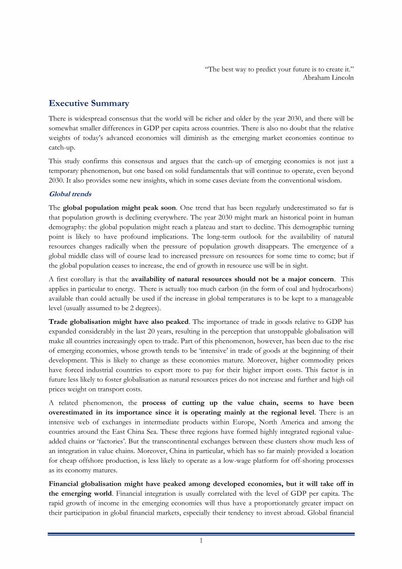
Even with a stable global population, however, some important differences across regions will remain.
The ‘fertility map’ of the world produced by the UN Population Division, shown in Figure 2.2, shows
that most continents are already close to replacement fertility, including North America and Asia. Europe
is now below that level. Only Africa has very high fertility, displaying even higher values in the sub-
Saharan region (SSA).
4 See Bongaarts & Bulatao (2002) for a more detailed discussion. 5 In The Population Bomb, Paul R. Ehrlich warned in 1968 of mass starvation in the 1970s and 1980s due to overpopulation, as well as other major societal upheavals, and advocated immediate action to limit population growth. Fears of a ‘population explosion’ were also present in the 1950s and 1960s, but this book and its author brought the idea to a wider audience. 6 The country had earlier abandoned the policy for couples in which both partners were the only child and announced in November 2013 a relaxation of this policy for couples in which only one partner was an only child.
0
2,000
4,000
6,000
8,000
10,000
12,000
19
60
19
65
19
70
19
75
19
80
19
85
19
90
19
95
20
00
20
05
20
10
20
15
20
20
20
25
20
30
20
35
20
40
20
45
20
50
Medium fertility
Low fertility
High fertility
Past
Today 2030
The Global Economy in 2030: Trends and Strategies for Europe
10
Figure 2.2 Fertility rates across continents (2012)
Source: UN Population Division.
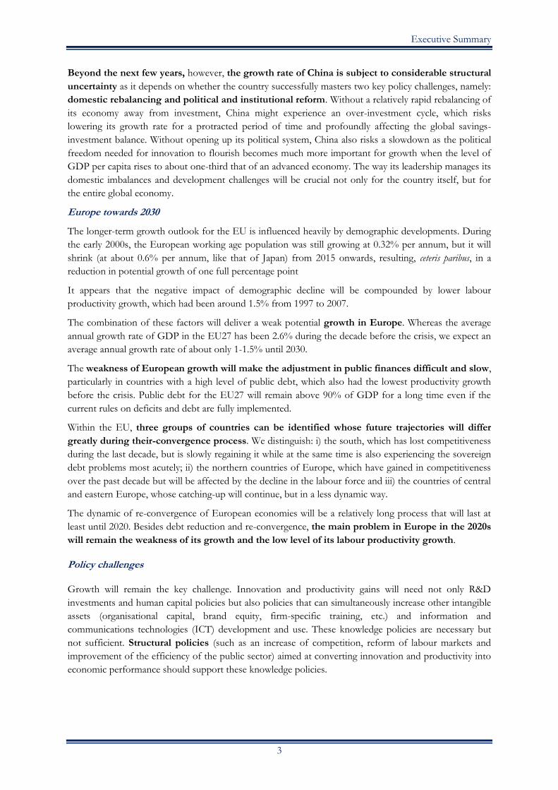
This means that most of the population growth in the future, whatever the rate, will come from
developing and emerging countries, especially SSA,7 which might be the only major region with
significant population growth by 2030. As suggested by Figure 2.3, in 2030 Asia will remain the most
populous region, but not the youngest; its median age will be well above the level of Africa but also that
of Latin America. Europe will definitely have the oldest population in the world.
Figure 2.3 Population by continent and median age, projections for 2030 (mil.)
Source: UN Population Division.
2.1.1 Demographic transitions
The transition from a regime of high mortality and fertility to one of low rates is a well-established
phenomenon observed in many empirical studies. During the first stage of the transition, the share of the
working-age population in the total population increases. This is a positive development as it improves,
ceteris paribus, per capita income. As long as output per worker, labour force participation rates and
7 This does not mean that fertility rates will remain as high as they are today. UN projections expect the rates to fall quickly from above 5 today, down to below 3.5 in 2025-30 under the low variant scenario (4.4 in the high projection). This will result in a youth bulge by around 2030.
Part I. Global Drivers of Growth
11
employment rates do not deteriorate, a rise in the share of the working-age population leads to an
increase in output per capita, which is often called the ‘demographic dividend’. Regions like SSA or India
are entering this phase, which should improve their growth prospects.
The advanced countries are in a much more advanced stage of demographic transition. They experienced
a temporary increase in fertility after the end of the Second World War, but then in the 1970s the birth
rate started to fall. This gave the advanced countries their own, temporary, demographic dividend as the
number of workers available to support the young and the very old increased. This increase in the so-
called ‘support ratio’ (or the inverse of the old dependency ratio) made gains in income per capita easier
to achieve for a time. However, a generation or two after the fall in birth rates (in the 1990s and 2000s),
the support ratio was negatively affected.
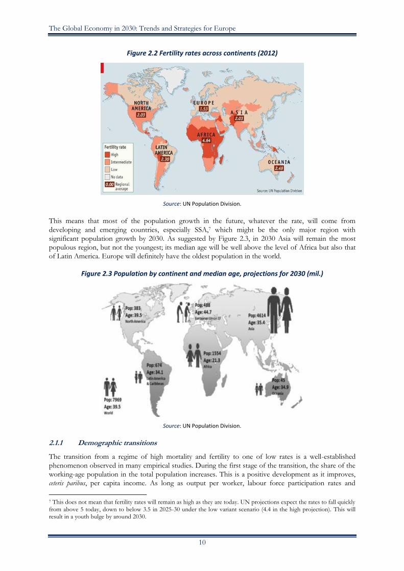
These demographic developments take decades to fully play out, but there is evidence that the turning
points can have considerable economic importance since peaks in the support ratio have often coincided
with major long-term turning points for the economy. Magnus (2013) argues that peaks of the support
ratio coincided with booms and busts in economic growth (and in asset markets). Figure 2.4 shows that
the support ratio peaked at close to 2.4 in Japan around 1990, coinciding with the peak of the Japanese
bubble. The ratio then fell continuously in Japan, but continued to increase in the US and Europe. The
peaks for the US and Europe (around 2010 and 2015, respectively) are less marked than for Japan, but the
fact that the support ratio will continuously decline implies that gains in income per capita will become
harder to achieve. A period of prolonged weakness thus becomes more likely.
Figure 2.4 Total support ratio (working age population per total dependents) of boom to bust
Note: Support ratio is defined as ratio of working age population to dependents.
Source: Authors’ own elaboration based on UN data.
As argued by Magnus (2013), one of the most significant factors in the rise of the support ratio was the
influx of women into the labour force, which, in turn, was probably connected with the decline in fertility
rates. As this factor has now most likely reached a plateau, the main impact on the support ratio comes
from the rapid ageing of the population. A decline in the European support ratio from about 2.2 in 2010
to 1.6 in 2030 would imply a fall of about 1.5% per year over the next 17 years. This implies that GDP
per capita might remain stagnant even if the productivity per worker increases by 1.5% per year. Until
(around) 2010, the demographic dividend had operated in the opposite direction as the support ratio had
been increasing by almost one percentage point per year. The negative impact from pure demographic
factors will thus be substantial in both Europe and the US. At an unchanged rate of productivity increase
per worker, the negative impact on the growth rate of GDP per capita will fall by over two percentage
points.
0.000
0.500
1.000
1.500
2.000
2.500
3.000
3.500
4.000
19
60
19
65
19
70
19
75
19
80
19
85
19
90
19
95
20
00
20
05
20
10
20
15
20
20
20
25
20
30
20
35
20
40
20
45
20
50
CHN IND JPN USA Europe SSA
Japan crisis EU & US crisis
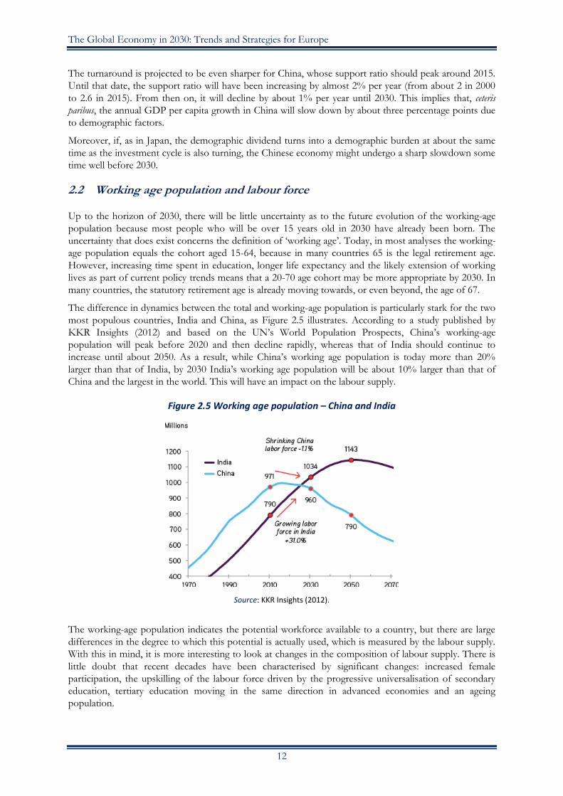
The Global Economy in 2030: Trends and Strategies for Europe
12
The turnaround is projected to be even sharper for China, whose support ratio should peak around 2015.
Until that date, the support ratio will have been increasing by almost 2% per year (from about 2 in 2000
to 2.6 in 2015). From then on, it will decline by about 1% per year until 2030. This implies that, ceteris
paribus, the annual GDP per capita growth in China will slow down by about three percentage points due
to demographic factors.
Moreover, if, as in Japan, the demographic dividend turns into a demographic burden at about the same
time as the investment cycle is also turning, the Chinese economy might undergo a sharp slowdown some
time well before 2030.
2.2 Working age population and labour force
Up to the horizon of 2030, there will be little uncertainty as to the future evolution of the working-age
population because most people who will be over 15 years old in 2030 have already been born. The
uncertainty that does exist concerns the definition of ‘working age’. Today, in most analyses the working-
age population equals the cohort aged 15-64, because in many countries 65 is the legal retirement age.
However, increasing time spent in education, longer life expectancy and the likely extension of working
lives as part of current policy trends means that a 20-70 age cohort may be more appropriate by 2030. In
many countries, the statutory retirement age is already moving towards, or even beyond, the age of 67.
The difference in dynamics between the total and working-age population is particularly stark for the two
most populous countries, India and China, as Figure 2.5 illustrates. According to a study published by
KKR Insights (2012) and based on the UN’s World Population Prospects, China’s working-age
population will peak before 2020 and then decline rapidly, whereas that of India should continue to
increase until about 2050. As a result, while China’s working age population is today more than 20%
larger than that of India, by 2030 India’s working age population will be about 10% larger than that of
China and the largest in the world. This will have an impact on the labour supply.
Figure 2.5 Working age population – China and India
Source: KKR Insights (2012).
The working-age population indicates the potential workforce available to a country, but there are large
differences in the degree to which this potential is actually used, which is measured by the labour supply.
With this in mind, it is more interesting to look at changes in the composition of labour supply. There is
little doubt that recent decades have been characterised by significant changes: increased female
participation, the upskilling of the labour force driven by the progressive universalisation of secondary
education, tertiary education moving in the same direction in advanced economies and an ageing
population.

Part I. Global Drivers of Growth
13
Figure 2.6 Changes in the global labour force (1980-2030)
(a) Total labour force (millions) (b) Female participation rates
Source: MaGE estimations and projections.
The average labour force participation of women in the US was 20% at the beginning of the 20th century
(Costa, 2000); as shown in Figure 2.6, it is now close to 60%. Currently, activity rates of women is above
50% in many advanced economies, with the exception of laggards like Italy, where the percentage is still
only 44%, and leading countries like Sweden and Denmark, which reached 67% in 2010. The increase was
the result of changes in social attitudes and fertility decisions on the one hand, and innovations that
increase the productivity of housework on the other. Wider female participation in schooling and the
tertiarisation of the economy (i.e. development of the services sector) have also played a fundamental
role, by increasing the opportunity cost of not entering the labour market and by creating housework-
friendly occupations.8
In some European countries like Poland and Italy, there is still the potential for catch-up, and these are
indeed the countries where an improvement has been observed in recent years. In the frontrunner
countries, however, progress has been modest, signalling that a plateau may have been reached.9 Future
developments up to 2030 could therefore include a convergence in Europe towards levels currently
observed in frontrunners (up to 65%), but any further increase to reach the level of male participation
(70% on average in the EU in 2010) is unlikely.
One aspect to be considered is that higher educational levels increase the opportunity costs of not entering
the labour market, and provide an argument against a decline in participation. Our global model, MaGE,
incorporates these mechanisms and, as illustrated in Figure 2.6 (panel b), predicts substantial increases in
female labour force participation for India, Korea, the Middle East and North Africa (MENA) and SSA,
whereas a slight decrease is foreseen for China and also for Europe and the US. The latter result, which
may appear counter-intuitive at first glance, is due to the fact that the positive relationship between
education and labour activation is strong for prime-age women but does not hold true for the oldest and
youngest cohorts, which are increasingly likely to still be in education.
2.3 Quantity versus quality
The potential for economic growth depends not only, or even mainly, on the number of workers in the
labour force, but on their quality (i.e. their level of education). It is widely agreed among policy-makers
8 For a review of the literature, see Cipollone et al. (2012) and Lewandowski et al. (2013). 9 Fortin (2009).
30%
35%
40%
45%
50%
55%
60%
65%
70%
75%
1980 1990 2000 2010 2020 2030
(% o
f to
tal f
em
ale
po
pu
lati
on
)
US CHN IND
JPN EU SSA
0
100
200
300
400
500
600
700
800
900
1980 1990 2000 2010 2020 2030
US CHN IND
JPN EU27 SSA

The Global Economy in 2030: Trends and Strategies for Europe
14
and experts that education plays a fundamental role as an engine of economic growth, with important
spillovers beyond the pure economic sphere. Sustained educational expansion has characterised advanced
economies’ policies since the post-war period. While national systems initially focused on primary and
secondary education, upskilling today concerns an ever-greater portion of high-school graduates enrolling
in university.
For many years the US had been the leader in this development, but the data show that there has been a
process of convergence between Europe and the US, especially in the last decade. Many European
countries are likely to achieve, and even exceed, the EU2020 target of 40% of the cohorts aged 30 to 34
completing tertiary education.
Economic theory and empirical studies emphasise the importance of tertiary educational attainment in
advanced economies. As argued by Aghion et al. (2006), a highly skilled labour force (meaning with
tertiary education attainment) enhances productivity growth more significantly for countries that are
closer to the technological frontier. This happens because high-skilled labour is better equipped to
generate innovation at the frontier, whereas lower-skilled labour is better suited to imitation. University
education is, in this sense, fundamental to the creation and implementation of innovation. The model we
used is consistent with this theory: the growth in total factor productivity (TFP) is expressed as a function
of the share of working-age population that completed secondary and tertiary education. Secondary
education is also considered important for its role in technology diffusion. The assumption is that an
increase in tertiary education of 10% raises TFP growth by 0.5%.
In principle, one should thus just need to look at the data on tertiary education to be able to gauge the
potential of a country to innovate and to experience TFP growth. In reality, however, different sources
provide quite different numbers, in some cases so different that they would lead to quite different
conclusions. This applies in particular to Europe and China. For both areas, the most widely used
international dataset paints a quite different picture if compared to the official statistics of the two
regions. In this case, data consistency is not just a bone of contention between experts, since a clearer
picture of the true state of affairs has important implications for economic-policy strategy.
As far as the EU is concerned, Eurostat reports that the five biggest economies (the Big 5) – Germany,
France, the United Kingdom, Italy and Spain – have graduation rates of around 25%, but the standard
global source, namely Barro & Lee (forthcoming), has only 12% for the same countries, less than half as
much. Moreover, according to the Barro & Lee figures, the share of the total population with a tertiary
degree is almost three times higher in the US than in Europe, whereas the gap is much narrower
according to European figures (which also imply that the difference between the graduation rates of the
younger cohorts in the US and the EU’s Big 5 is now very small).
These differences in data concerning tertiary education are significant when assessing whether Europe
can catch up with the per capita income of the US. Eurostat data would suggest that the difference in
education levels is narrowing rather quickly, which should allow the EU to reach US levels of income per
capita, provided, of course, that the potential human capital is used efficiently in Europe.
Regarding China, the data discrepancies are even starker. For example, a 2010 Chinese government plan
for medium- and long-term education reform implies a total number of people with a higher education of
98 million in 2009, which would be approximately three times the estimates of Barro & Lee. The official
objective is to double that amount by 2020; the share of those who received higher education would then
amount to over 20% of the population aged 20-59. The Chinese Ministry of Education reported that
already in 2013 approximately 7 million new graduates entered the labour market. This would correspond
to a tertiary graduation rate of about 30%, given an annual cohort size of slightly above 20 million.
One view of China would be that even by 2030, the country will still have an ‘elite’ tertiary education
system, limiting the ability of the country to become an important centre of innovation. The alternative
view (consistent with the plans of the political leadership) would be that by the same time horizon,
tertiary education will have been extended to the masses to provide the country with the necessary
conditions to become an innovator on its own.

Part I. Global Drivers of Growth
15
We do not accept this optimistic view of China in our analysis, but given the central role of tertiary
education for growth, an alternative scenario was run in order to quantitatively evaluate the impact of a
faster educational expansion. In this alternative scenario, the speed of the catch-up with the global leader
(the US) has been doubled relative to the rather slow adjustment path that can be expected based on past
data. As shown in Figure 2.8, this would imply that the share of the working-age population with a
completed tertiary degree increases much faster than in the central scenario and by 2030 reaches 40%
(instead of 31%) for Europe, 17% (instead of 12%) for China and India, but remains below 10% in SSA.
In this scenario, the catch-up of all major emerging markets would be stronger and the EU would also
experience a higher growth of about 0.5% per year due mainly to faster productivity growth.
Figure 2.7 Paths of tertiary education
expansion: MaGE Central scenario
Figure 2.8 Paths of tertiary education expansion:
MaGE alternative scenario
Source: MaGE estimations and projections.
2.4 Migration
Migration is a complex part of regional population forecasts, even though it obviously does not change
the global population. Migration is a particularly important issue for Europe but very difficult to forecast
with accuracy; hence it might be more useful to understand how the traditional factors that determine
migration are likely to evolve.
The three main push factors of migration are well known: i) income differentials between the country of
destination and the country of origin, ii) the level of education of the potential migrant and iii) his/her
age.10 Most empirical studies focus on the first two, taking the younger cohorts as the potential migrants.
Income in the destination country compared to the one of origin (combined with the probability of
employment) remains then the key element, together with the cost of migration. Mansoor & Quillin
(2007) estimate that for migration to be economically attractive, a wage differential of at least 30-40% is
necessary between the country of origin and the destination country.11 This provides a useful reference to
gauge future migratory pressure. The model we used predicts that the income distance between Europe
and the developing economies, in terms of GDP per worker (PPP), will shrink considerably. In Figure 2.9
we consider some important sending regions.
10 Age and education are individual features that influence the decision to emigrate. Young, educated people are generally more mobile. As the fertility rate is falling significantly in the MENA region, the North-African ‘youth bulge’ may vanish and the flows of migrants from that region into Europe may decline substantially. 11 According to Mayda (2005), a 10% increase in the level of GDP per-worker in the destination country increases emigration on the order of 2.6 per 100,000 individuals in the origin country.
0%
10%
20%
30%
40%
50%
60%
70%
1980 1990 2000 2010 2020 2030
(% o
f to
tal p
op
ula
tio
n)
US CHN IND
JPN EU SSA
0%
10%
20%
30%
40%
50%
60%
70%
1980 1990 2000 2010 2020 2030
(% o
f to
tal p
op
ula
tio
n)
US CHN IND
JPN EU SSA

The Global Economy in 2030: Trends and Strategies for Europe
16
The key result is that even by 2030, output per worker will be only 10% of the European level in SSA,
30% in North Africa (NAF), 22% in India, 40% in South America (SAM) and 81% in Turkey. As a
consequence, if only the economic aspect is taken into account as a push factor, much less immigration
can be expected from Turkey and South America, and more from the remaining areas, especially sub-
Saharan Africa.
Figure 2.9 Income differentials in 2030: Average GDP per worker
as % of EU average in selected regions
Note: SAM = South America, SSA = Sub-Saharan Africa, NAF = North Africa, IND = India and RoA = Rest of Asia.
Source: MaGE estimations and projections.
The OECD (2009) has a similar result, predicting that by 2030 income convergence across countries will
have reduced the relative attractiveness of today’s advanced economies. The flows that seem most
important today (e.g. from Turkey to Germany, or Mexico to the US) might no longer be as important as
those to new poles of attraction in Asia, such as Japan or Korea.
The migratory pressure from North Africa should remain, but diminish somewhat. Indeed, this future
seems to be with us already. According to Eurostat, Africa already provides one-quarter of the total
citizens of non-EU countries resident in the EU – a percentage that is likely to increase. To assess the
potential impact of increased migration, the alternative scenario we analysed assumes the entry of an
additional 2 million migrants (compared to the central scenario) between 2010 and 2030, adding to the
stock of approximately 20 million of today’s non-European foreign residents.12 It turns out that this
increase in migration would not substantially alter the path of the European economy.
2.5 Urbanisation
For the first time in history, more than 50% of the world's population live in urban areas.13
Demographers estimate that even in Africa, half the population will live in cities by 203014 and Asia will
be home to more than 50% of the world’s urban population in a long-term horizon (2050). By contrast,
Europe's urban population as a percentage of the global total is likely to have shrunk considerably. Figure
12 According to the latest Eurostat figures on statistics, the foreign population (people residing in an EU27 member state with citizenship of a non-EU27 member state) on 1 January 2012 was 20.7 million, representing 4.1% of the EU27 population. To this one should add 13.6 million persons living in one of the EU27 member states with citizenship of another EU27 member state on 1 January 2012. 13 Defining ‘urban’ has been a difficult task and there is no commonly agreed definition. Each country defines urban in its own way and this can refer to cities, towns, villages, conurbations or localities. There are a number of approaches in which criteria are used to determine what an urban area is. 14 McKinsey Global Institute (2010).
0%
10%
20%
30%
40%
50%
60%
70%
80%
90%
SAM SSA NAF IND RoA Turkey
2012
2030
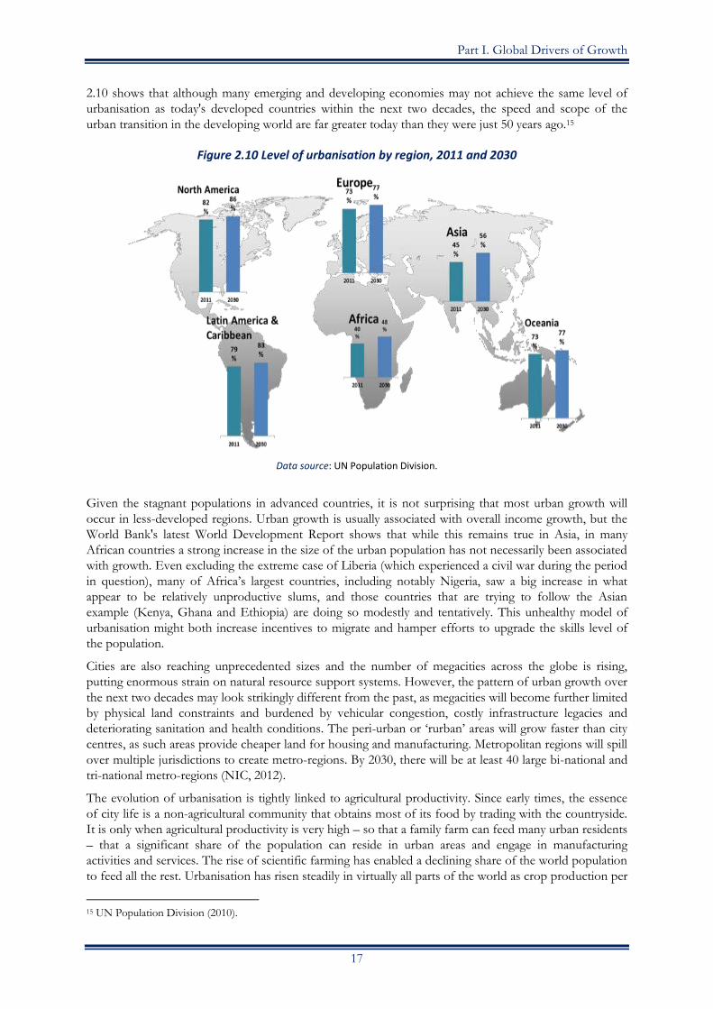
Part I. Global Drivers of Growth
17
2.10 shows that although many emerging and developing economies may not achieve the same level of
urbanisation as today's developed countries within the next two decades, the speed and scope of the
urban transition in the developing world are far greater today than they were just 50 years ago.15
Figure 2.10 Level of urbanisation by region, 2011 and 2030
Data source: UN Population Division.
Given the stagnant populations in advanced countries, it is not surprising that most urban growth will
occur in less-developed regions. Urban growth is usually associated with overall income growth, but the
World Bank's latest World Development Report shows that while this remains true in Asia, in many
African countries a strong increase in the size of the urban population has not necessarily been associated
with growth. Even excluding the extreme case of Liberia (which experienced a civil war during the period
in question), many of Africa’s largest countries, including notably Nigeria, saw a big increase in what
appear to be relatively unproductive slums, and those countries that are trying to follow the Asian
example (Kenya, Ghana and Ethiopia) are doing so modestly and tentatively. This unhealthy model of
urbanisation might both increase incentives to migrate and hamper efforts to upgrade the skills level of
the population.
Cities are also reaching unprecedented sizes and the number of megacities across the globe is rising,
putting enormous strain on natural resource support systems. However, the pattern of urban growth over
the next two decades may look strikingly different from the past, as megacities will become further limited
by physical land constraints and burdened by vehicular congestion, costly infrastructure legacies and
deteriorating sanitation and health conditions. The peri-urban or ‘rurban’ areas will grow faster than city
centres, as such areas provide cheaper land for housing and manufacturing. Metropolitan regions will spill
over multiple jurisdictions to create metro-regions. By 2030, there will be at least 40 large bi-national and
tri-national metro-regions (NIC, 2012).
The evolution of urbanisation is tightly linked to agricultural productivity. Since early times, the essence
of city life is a non-agricultural community that obtains most of its food by trading with the countryside.
It is only when agricultural productivity is very high – so that a family farm can feed many urban residents
– that a significant share of the population can reside in urban areas and engage in manufacturing
activities and services. The rise of scientific farming has enabled a declining share of the world population
to feed all the rest. Urbanisation has risen steadily in virtually all parts of the world as crop production per
15 UN Population Division (2010).

The Global Economy in 2030: Trends and Strategies for Europe
18
hectare, and more importantly, crop production per family has continued to rise over time. For instance,
in the US, with its enormous output per farmer (due to both high productivity per land area and large area
per farm), farming families constitute just 1% of the population but are able to feed the other 99%.
Urbanisation is closely linked to the driver of rural-urban migration. One important driver is high fertility
rates in many rural areas, combined with limited employment opportunities, particularly from the
marginalisation of small farmers. Urban areas offer better jobs and educational opportunities. These
conditions represent an incentive for rural residents to seek a better life and a higher income in urban
areas.
Last but not least, there is an important cause-and-effect nexus between urbanisation and economic
growth, as the largest share of infrastructure investments – especially in China and other emerging
countries – is concentrated in cities. Urbanisation has worked as one of the main sources of domestic
demand in emerging countries, through higher consumption of a growing affluent middle class and very
high spending in infrastructure. This process is expected to continue in the future.16
Figure 2.11 Urbanisation and income (change between 1985 and 2010)
Source: World Bank.
The World Bank’s World Development Report 2012 shows the processes at work in Asian countries in
1985 to 2010. But general rules are made to be broken. As the right half of Figure 2.11 shows, in many
African countries an increase in the size of the urban population has not necessarily been associated with
growth. Excluding the extreme case of Liberia (which had a civil war during the period in question), many
of Africa’s largest countries, notably Nigeria, saw a big increase in what appear to be relatively
unproductive slums, and those countries that are following the Asian example (Kenya, Ghana and
Ethiopia) are doing so modestly and tentatively. The report examines the role of job creation in
development, and suggests that while policies to encourage jobs and to foster growth are similar, they are
not identical.
16 The target of the Chinese government is to transform 60% of the population of almost 1.4 billion into urban residents by 2020. Plans to build homes, roads, hospitals and schools for them are already in place.

Part I. Global Drivers of Growth
19
3. Capital and capital markets
A high rate of investment in physical capital is one of the key conditions for growth. Over the last two
decades, a clear-cut global trend has been the increase in the rate of capital accumulation, which has been
accompanied by the expansion of the financial system in general.
The expansion of finance appeared to have worked as an additional factor of growth, but the crisis of
2008-09 suggests that this was an illusion created by the credit boom. While the key function of finance is
to channel savings into the best investment projects, events since 2007-08 reveal that the financial system
has not always been able to find the best investment opportunities.
In advanced economies, more finance has been flowing, but alongside less investment. It is difficult to say
whether this combination can and will continue until 2030. Experience of aftermaths of systemic financial
and debt crises suggests that deleveraging might have a prolonged negative impact on growth and
investment. Uncertainty in this area remains high, however, because a relapse of the euro crisis could
reinforce this tendency, whereas a quick return of confidence and a strengthening of the euro area’s
banking system might result in investment recovering more strongly. The model we use assumes that
these problems will be overcome rapidly and that investment and savings will soon be determined again
by fundamental factors, such as ageing.
3.1 Investment and capital accumulation as drivers of growth
The global average investment rate in physical capital has increased considerably over the last decade to
reach about 28% of GDP, whereas it was only 21-22% of GDP during the early 2000s. But investment
rates have diverged across major regions, increasing considerably in the emerging economies and
stagnating or even falling in the advanced countries. The investment rate in emerging countries now
stands at about 33% of GDP, while the great financial crisis has led to a sharp fall in investment in
advanced economies, reinforcing its longer-term trend. The result is that investment in the EU and the
US is substantially below 20% of GDP, heading towards 15%. The projections of the model used here
suggest that investment in advanced countries should recover to a level somewhat below that observed
before the crisis, but then resume its decline. Much larger falls in investment rates (as a share of GDP) are
expected in two key emerging economies, namely China and India. See Figure 3.1.
Figure 3.1 Regional investment (% of GDP)
Source: MaGE projections.
10%
20%
30%
40%
50%
1980 1990 2000 2010 2020 2030
US CHN IND JPN EU27 SSA

The Global Economy in 2030: Trends and Strategies for Europe
20
Such predictions about emerging markets contrast with the more short-run projections of the IMF,
according to which the investment rate for China should remain above 45% of GDP until the end of the
current decade, instead of the 35% predicted by the model. The model thus assumes that the re-balancing
of the Chinese economy away from consumption (and exports) will take place rather rapidly. This is not
only the Chinese government’s official goal; putting the Chinese economy on a sustainable basis is also
widely seen as necessary. The model calculates such a sustainable path and in this it differs from mere
trend extrapolation, which in this case would lead to huge imbalances.
Given the rising weight of the emerging market economies, an increasing part of global investment will
take place there and their capital stock will be newer than that of advanced economies. The World Bank
(2013a) calculates that in a few years total investment in developing countries should exceed that of
(today’s) high-income countries and that by 2030, the share of developing countries in the global total
should go above 60%. This prediction stands in stark contrast to the situation until about 2000, when
developing countries accounted for a little over 20% of total global investment.17
3.2 The longer-term effects of high investment rates
Standard economic theory holds that investment can be a key driver of growth, but that this effect is only
temporary. An increase in the rate of investment will thus lead initially to a higher growth rate, both
because investment itself is part of aggregate demand and because a higher capital stock increases
potential output. However, once a higher capital stock has been reached, output will stop growing. In the
long run, a higher investment rate will thus result mainly in a higher stock of capital and a higher level of
output per capita, but not in a permanently higher growth rate.
Moreover, the available empirical evidence indicates that increasing the capital stock per worker leads to
rapidly decreasing returns, implying that after a certain level even a much higher investment effort will not
result in a much higher level of output per worker once the transition period has ended. The transition
period during which higher investment still has a strong impact on growth can be rather long – easily a
decade or more – depending on the starting point.
These two indications, namely that higher investment leads only temporarily to higher growth and that
the transition period can last a long time, constitute a key to understanding global growth dynamics and
the potential dangers of overinvestment cycles for financial stability, as the experience of Japan has
shown. We will argue that a similar over-investment cycle might well arise in China – with potentially
significant consequences for global capital markets.
One key difference between emerging and advanced economies today is the amount of capital available
for each worker. The speed of convergence in this key variable is determined by the difference in the
investment rate (population growth differences are minor, except for sub-Saharan Africa).
As explained above, the model predicts that emerging countries can be expected to maintain a rather high
rate of capital accumulation, even if markedly lower than their present rates. The global capital stock will
thus continue to increase. China exhibits an exponential increase of capital stock, which will reach the
level of the US or the EU by around 2030, even if the investment rate declines considerably from today’s
level. This larger total capital stock is, of course, distributed over a much larger workforce. For most other
countries, the capital stock will increase only moderately, as a large part of investment is needed just to
offset depreciation on the existing stock. The EU’s capital stock will remain above the US levels as its
investment rate is also projected to remain higher. Japan is a special case, with an almost-flat path for
capital stock.
17 The World Bank (2013) report also shows that China alone accounts for well over half of all global investments in manufacturing, implying that a dominant share of the global capital stock will be in this country by 2030.

Part I. Global Drivers of Growth
21
Figure 3.2 Capital stocks
($ billion, 2005 dollars)
Figure 3.3 Capital intensity per capita
(thousands of 2005 US dollars)
Source: MaGE estimations and projections. Source: MaGE estimations and projections.
In terms of distribution of capital, according to World Bank (2013a) estimates, over one-half of the total
capital stock will be in developing economies by 2030.
The key variable for productivity (not growth), however, is not the total capital stock, but the stock per
worker (economists call this ‘capital intensity’, or the capital to labour ratio (K/L). The projections of the
model, shown in Figure 3.3, suggest that the distance in capital/labour ratios between the ‘leaders’ (Japan,
the EU and the US) and the rest cannot be overcome until 2030, given the size of the gulf today. Despite
investment rates of above 30% of GDP, the ratio of China’s capital-to-labour will reach only one-quarter
of the US or EU level in 2030, although, as shown above, the total capital stock of the country will be
approximately as large as that of the US or the EU. This is because the labour force of China is about
three to four times larger than that of the EU.18
Japan is also a special case with respect to its capital intensity, which is not only high, but continues to
increase because the workforce is declining so rapidly. The leading position of Japan for capital intensity
therefore remains unchallenged. However, the implication of this primacy is higher wage rates and not a
higher growth rate.
The considerable narrowing of the gap in capital-to-labour ratios should go hand-in-hand with a
narrowing in the gap in wages, as the capital labour ratio is a key determinant of labour productivity. A
clear difference in wage rates between emerging and advanced economies will thus remain until 2030, but
it will be much less significant than it is today.
3.3 Savings versus investment
In the end, all investment has to be financed by savings. This is by definition true at the global level: ex
post the global investment rate has to equal the global savings rate. However, this does not hold true at
the level of each individual country or economy, as the difference between savings and investment is
equal to the current account balance of the country.
18 It is clear that China’s capital-to-labour ratio would get much closer to that of the EU if the country were to maintain its current investment rate of over 45% of GDP.
0
10,000
20,000
30,000
40,000
50,000
60,000
1980 1985 1990 1995 2000 2005 2010 2015 2020 2025 2030
US CHN IND
JPN EU SSA
0
50
100
150
200
250
300
350
1980 1985 1990 1995 2000 2005 2010 2015 2020 2025 2030
US CHN IND
JPN EU SSA

The Global Economy in 2030: Trends and Strategies for Europe
22
A simplistic view of the global economy would suggest that the rich and ageing advanced countries
should finance the build-up of the capital stock in the poorer parts of the world. The reality is different,
however. The emerging economies have increased their savings rates even more than their investment
rates with the result that over the last decade emerging markets have, on average, run current-account
surpluses.
In the MaGE model, large current-account imbalances are gradually eliminated over time, based on the
idea that large current-account deficits are not sustainable. In the longer run, this implies that savings and
investment rates follow a similar path at the national level. Figure 3.1 above, to a first order of
approximation, depicts not only investment but also the evolution of savings, which are expected to
remain much higher in emerging economies. This is consistent with projections of the World Bank
indicating that an increasing share of global savings (over 60%) will be generated in emerging countries.19
3.4 Finance: A roadblock to recovery or a necessary ingredient of development?
The role of the financial sector is to connect savers to investment opportunities. In this sense finance per
se does not constitute a driver of longer-term growth, but when the financial system fails to work it can
constitute an obstacle to growth. Nevertheless, an efficient financial system that selects the best
investment projects can sustain growth for some time.
The great financial crisis has led to a new wave of empirical research that re-examines the link between
finance and growth (which previously has been believed in general to be positive). Some of these studies
find evidence of a non-linear relationship between finance and growth, implying that that there is a
threshold, typically of around 100% of credit-to-GDP, beyond which a larger financial sector no longer
fosters economic growth.20 However, the reasons why a very large financial sector might dampen
economic growth are poorly understood.
We do not take a stance on this issue, but we observe that there is a strong relationship between the level
of development as measured by GDP per capita and the size of the financial system. This is related to the
regularity, observed in the chapter on globalisation, with which the size of outward financial investments,
especially FDI, is also positively related to GDP per capita. Both trends are also carefully documented by
the World Bank (2013a).
The combination of rapid growth and the tendency of a financial sector to expand relative to income as
GDP per capita increases imply that the financial sector in emerging economies must be expected to
grow by much more than nominal GDP in these countries. Given that the financial sector is retrenching
in most advanced countries, it follows that one can expect a very rapid shift in the locus of financial
activity towards emerging economies.
Here again, one has to distinguish between stocks and flows. The rate of growth of finance will be vastly
greater in emerging economies and they will soon account for a majority of the flow of savings. But
today’s advanced countries still account for the vast majority of the stock of global financial wealth. It will
take some time before similarly-sized stocks will be built up in many emerging economies.
Rapid growth of financial activity rarely materialises without eventual financial crisis. This danger is
especially acute in emerging countries, whose financial markets are often opaque and dominated by banks,
complemented by other intermediaries that perform bank-like activities. One should thus expect a
number of financial crises over the next decade. Experience has shown that financial crises are more
virulent in countries that depend on foreign capital inflows. This is not to say that countries with strong
external balance sheets cannot experience financial crises (Japan is a major case in point). But these crises
tend to be less acute in the short run and the country in question does not usually need external support.
Emerging economies might thus increasingly fall into one of two different categories:
19 And about two-thirds of this will be generated in China. 20 See e.g. Cecchetti & Kharroubi (2012) and Panizza et al. (2012).

Part I. Global Drivers of Growth
23
i) Those with weak external balance sheets might suffer from a number of boom-bust cycles in
capital inflows, potentially requiring assistance from the IMF or the new, still untested, regional
financing arrangements, such as the Chiang Mai Initiative in Asia.21
ii) Those with strong external balance sheets (e.g. China) might also experience financial crises, but
they would not need external assistance and would, so to speak ‘suffer in silence’.
In the short run, Europe is facing the opposite problem, in that its financial system is in a deleveraging
phase. It is widely assumed that the reluctance of banks to extend credit will hamper the recovery. In
reality this hypothesis is not always supported by experience. Some new evidence22 suggests that declining
bank credit will not necessarily constrain recovery after output has bottomed out after a financial crisis.
3.5 Conclusions
Investment and capital markets are key determinants of the global economy. We find that investment will
definitely not act as a brake on growth. On the contrary, some emerging countries should reduce their
investment rates to avoid an excessive build-up of capital. But, even with strong investment in emerging
economies, this will only lead to a considerable narrowing, not a closure, of the huge gap that persists in
terms of capital-to-labour ratios today. Investment and savings will increasingly originate in emerging
economies and financial activity should expand more than proportionally to income in emerging markets.
It is thus the allocation of capital via financial markets that might constitute a problem. The extremely
rapid expansion of financial activity in emerging markets brings with it the potential for financial crisis,
which could become virulent in countries with weak external balances.
4. Globalisation
Globalisation can be described as “a widening, deepening and speeding up of worldwide
interconnectedness in all aspects of contemporary social life, from the cultural to the criminal, the
financial to the spiritual”.23 More specifically, economic globalisation refers to the greater global
connectedness of the production of goods and services (i.e. trade), as well as increasing flows of
investment (i.e. FDI). Globalisation has been the subject of intense debate over the last two decades
among experts and the general public alike, and it is widely considered a key driver of growth. Its
evolution is therefore of central importance to understanding the outlook for the global economy by
2030. This chapter presents evidence of past and emerging trends, stressing less conventional aspects of
both trade, in goods and services, and investment flows, FDI in particular. We then explore possible
future developments.
4.1 Trade
Undeniably, the importance of trade increased massively over the last two decades. The dotted line in
Figure 4.1 shows that the ratio of global exports to global GDP increased from just below 20% in the
early 1990s to over 30% at the peak of the global credit boom in 2007-08.
21
The Chiang Mai Initiative (CMI) is a multilateral currency swap arrangement among the ten members of the Association
of Southeast Asian Nations (ASEAN), the People's Republic of China (including Hong Kong), Japan, and South Korea. 22 See Takáts & Upper (2013). 23 Held et al. (1999, p. 2).

The Global Economy in 2030: Trends and Strategies for Europe
24
Figure 4.1 Global exports as percentage of world GDP (1980-2014)
Data source: IMF, World Economic Outlook.
The ensuing recession led to a sharp drop, followed by a partial recovery. IMF projections24 suggest that
this ratio should peak again by about 2018, although it is hard to tell whether the global recession of 2009
represented a real watershed or just a temporary interruption of a longer-term trend.
The dotted line in Figure 4.1 includes intra-EU trade which, in the context of the Single Market, can be
considered as internal trade, as can trade within the North Atlantic Free Trade Area (NAFTA). To isolate
regional integration, both components have been taken out. The result suggests that significant
integration has been taking place particularly at the regional level and for EU member states; the two
processes of economic ‘globalisation’ and ‘Europeanisation’ have proceeded in parallel.25
The impression of a rapidly integrating and globalising world economy partially derives from the fact that
trade strongly and directly affects manufactured goods, the most visible part of the economy, but one that
is declining. Figure 4.2 shows the ratio of exports of goods relative to manufacturing output for the three
largest mature economies: the US, the EU and Japan.26 This ratio, which has strongly increased over the
last two decades and is now close to 80%, is much higher than the ratio of goods exports relative to
GDP. This means that the importance of trade in the manufacturing sector has increased, while the
overall importance of the manufacturing sector in the economy has decreased, limiting the increase in the
share of trade in overall GDP.
By contrast, a comparison of exports as a percentage of GDP for the large economies and for the world
as a whole shows that trade is much less important in the former (around 10% of GDP compared with
over 20% for the world).
24 World Economic Outlook (WEO) database, April 2013. 25 We will document below that the integration within the EU has been complementary, leading to the emergence of what has been termed ‘factory Europe’. 26 Only extra-EU trade is considered in this case.
0%
5%
10%
15%
20%
25%
30%
35%
1980 1982 1984 1986 1988 1990 1992 1994 1996 1998 2000 2002 2004 2006 2008 2010 2012 2014
World exports as % of GDP
World exports minus intra-EU trade
World exports minus intra-EU & intra-NAFTA trade

Part I. Global Drivers of Growth
25
Figure 4.2 Comparison of exports in goods as a percentage of value-added in manufacturing and
GDP, Japan, US and EU27 (1998-2011)
(a) As % of value-added in manufacturing (b) As % of GDP
Note: For EU27: intra- and extra-EU exports.
Data sources: OECD and World Bank databases.
Figure 4.3 compares similar statistics for China with the average of the three big mature exporters (the
EU, the US and Japan). The two charts suggest that China stands out in terms of the share of exports of
goods in manufacturing (panel b), but is close to the mature economies in its exports relative to
manufacturing output (panel a). This is because the Chinese economy depends on manufacturing more
than other countries: its manufacturing sector represents over one-third of its total economy, compared
with less than one-sixth in the US and less than one-fifth in Europe.
Figure 4.3 Comparison of exports in goods relative to value-added in manufacturing and GDP,
China vs average of Japan, EU and US (1998-2011)
(a) As % of value-added in manufacturing (b) As % of GDP
Data sources: OECD and World Bank databases.
0%
10%
20%
30%
40%
50%
60%
70%
80%
90%
19
98
19
99
20
00
20
01
20
02
20
03
20
04
20
05
20
06
20
07
20
08
20
09
20
10
20
11
Japan USA EU27
0%
10%
20%
30%
40%
50%
60%
70%
80%
90%
19
98
19
99
20
00
20
01
20
02
20
03
20
04
20
05
20
06
20
07
20
08
20
09
20
10
20
11
Japan USA EU
0%
20%
40%
60%
80%
100%
120%
19
98
19
99
20
00
20
01
20
02
20
03
20
04
20
05
20
06
20
07
20
08
20
09
20
10
20
11
China Average JP, EU & US
0%
5%
10%
15%
20%
25%
30%
35%
40%
19
98
19
99
20
00
20
01
20
02
20
03
20
04
20
05
20
06
20
07
20
08
20
09
20
10
20
11
China Average JP, EU & US

The Global Economy in 2030: Trends and Strategies for Europe
26
4.1.1 Globalisation of services?
So far there is little evidence of globalisation in the services sector. The ratio of services exports to the
value of services output in the US, the EU and Japan is 5%, compared with almost 80% for
manufacturing. This suggests that while for industry ‘the world is flat’, it is certainly not yet the case for
services.
Overall, there is little doubt that the ratio of total trade (goods and services) to GDP has increased in the
past and it is tempting to assume that the trend observed between 1990 and 2007-08 will continue. Yet it
seems likely that the potential for goods trade has been at least partially exhausted.
When it comes to services, data suggest their direct trade is still relatively small: services trade is still worth
still only about 30% of goods trade for most countries, including within the EU. It should be recognised
however, that trade in goods incorporates to a large extent the value-added created by services sectors
such as business services and transport. It is therefore likely that trade in services will continue to increase
faster than trade in goods, thanks also to the liberalisation of the sector and the fact that services make up
an ever-increasing part of GDP. Moreover, progress in ICT has made it easier to exchange certain
services across borders, notably in the area of business. But this growth will be from a relatively small
base.
4.1.2 The predictions of the model
We used the MIRAGE model to simulate the size and direction of future trade flows based on the
evolution of GDP and its main components, such as industry, manufacturing and services. The main
conclusion from the simulation is that while trade will continue to play a very important role in the global
economy, its importance is unlikely to increase at the same pace as it has up to now, although services
offer the potential for important developments.
The advantage of using a fully-specified model is that it elucidates a general phenomenon that has
contributed to the overestimation of the extent of globalisation. It is often asserted, correctly, that over
the last 30 to 40 years the growth of the volume of international trade has always outpaced the growth of
real GDP. This is correct, but this observation is less relevant than it appears at first sight because the
relative price of the (still mainly) goods that are traded has fallen continuously, thus offsetting the
economic impact of the increase in the quantities exchanged. The model replicates this empirical
regularity and predicts that growth of trade will remain higher than GDP growth, but the difference is
expected to lessen over time towards 2030 (Figure 4.4). Moreover, given that the relative price of tradable
goods will continue to fall, the ratio of trade to GDP will not increase much, certainly much less than in
the past. The model thus suggests that the globalisation process, understood as a continuous rise in world
flows, is unlikely to continue at its previous pace.
The one economy that should be ‘de-globalising’ is China, whose export growth is set to decelerate
sharply, from 10.5% per year in value terms before the crisis to less than half of this value (4.1%) on
average for the period until 2030. Moreover, the difference between the growth rate of Chinese exports
and that of the world will shrink from 6.6 percentage points to 1.2 percentage points, meaning that the
share of Chinese exports in global trade will not increase much over the period up to 2030.27 The world in
27 By the year 2030, the growth rates of Chinese exports and world exports are projected to be exactly equal (in value terms). The difference between China and the rest of the world in terms of output growth rates will remain much higher (double at 2.6%) than the difference in export growth rates. This implies that there will be a sharp difference in the evolution of the share of Chinese GDP in world GDP (which is projected to increase considerably) and the share of China’s exports in world trade (which is projected to increase only marginally). At present, China’s share in global exports stands at around 9-10%, close to its share in global GDP. By 2030, the latter should have approximately doubled (in value

Part I. Global Drivers of Growth
27
2030 might thus be quite different from today in terms of GDP shares, but trade should not be more
dynamic than GDP and the dominant trading blocs should be the same as today: the EU, the US and
China.
Figure 4.4 World growth of output and exports
Note: Exports adjusted for intra-trade.
Source: MIRAGE results.
From an EU perspective, one should therefore ask which is more important: the increasing share of
China and other EMEs (emerging economies) in global GDP, or the fact that the trade of these new
powers is expanding much more slowly than before? Given that most of the external environment’s
influence on the EU will come via trade flows, one could argue that the challenges posed by the global
economy for the EU might be not very different from those of today.
It is thus not surprising that the model predicts that the shares of different trading partners will change
only moderately between now and 2013. As shown in Figure 4.5, under the central scenario, extra-EU
trade is projected to increase in importance relative to intra-EU trade, for the simple reason that the rest
of the world is growing more rapidly than the EU. On average, intra-EU trade today represents about
60% of all trade (and extra-EU trade, about 40%). These proportions are projected to reach an
approximate ratio of 50-50 by 2030.
The relative weights of the non-EU partners will shift in the expected direction, but not by very large
amounts, as the charts below show. However, one potentially important shift concerns the US and China.
The US is currently (2012 data), just the EU’s most important single trading partner (by decimal points
ahead of China). This will change by 2030 when China will be clearly the largest trading partner given that
its share in EU external trade will continue to increase, albeit at a slower pace than over the last decade.
Little change is expected for most other trading partners, except the ‘Rest of Europe’, which will decline
in importance given that it is also expected to grow more slowly than the rest of the world.
terms, i.e. including expected real appreciation), while China’s share of global exports should have increased by only about one-fifth, to roughly 12%.
3.70%
2.80% 2.80%
5.10%
3.80% 3.80%
0.0%
1.0%
2.0%
3.0%
4.0%
5.0%
6.0%
2005-07 2013-30 2030
GDP growth Export growth

The Global Economy in 2030: Trends and Strategies for Europe
28
Figure 4.5 EU27 trading partners, 2012 vs 2030
Note: RoW: Rest of World, CHN: China, JPN: Japan, KOR+TAI: Korea & Taiwan, IND: India, LA: Latin America,
RoE: Rest of Europe, RUS: Russia, TR: Turkey.
Date sources: Mirage results and EU TRADE statistics (Eurostat).
4.2 Global value-added chains: A revolution of trade patterns?
The discussion in the previous section concentrated on the most traditional indicator of trade, namely
that of trade in goods and services measured by the amount a country sells to or buys from abroad.
However, trade measured this way represents a gross, or ‘sales’, concept and is thus not directly
comparable to GDP, which quantifies the value-added created by an economy.
The empirical evidence for the supply chain phenomenon was until recently rather patchy. Recent work
by the WTO/OECD28 has, for the first time, provided reliable evidence at the macroeconomic and
industry level for a number of countries. These data confirm that the global supply chain (GVC)
phenomenon seems to be particularly strong in some industries (e.g. electronic). The best-known example
is Apple products, which appear to contain very little local Chinese value-added.29 This example might
not be characteristic of Chinese exports in general, however. Indeed, it is possible that the importance of
the global value chain (GVC) could be overrated and that the role of China in the chain is not limited to
the assembly of intermediate products. According to WTO/OECD research, the local value-added for
Chinese exports is actually around 70%, which is remarkably high for a country that is thought to provide
mainly assembly services (and an order of magnitude higher than the proportion suggested by the
example of Apple).
According to these recent statistics, it is true on the one hand that, for each individual EU member state,
a high proportion of foreign inputs are used in exports. On the other hand, most of this trade in
intermediate products takes place within the EU, which is seen as a ‘champion’ in the trade in
intermediates.30 If one considers the EU as a whole, the proportion of foreign (non-EU) inputs
incorporated into EU exports (to the rest of the world) is around 12%, which is a relatively small amount.
In this respect, EU industry is not unlike that of the US or Japan, implying that the GVC phenomenon
28 See OECD-WTO Trade in Value Added (TiVA) indicators. 29 See http://pcic.merage.uci.edu/papers/2011/Value_iPad_iPhone.pdf. 30 As reported in a WTO/JETRO (2010) report, with 41% of 2009 world exports in intermediates, followed by Asia with 35%.
RoW 25%
CHN 14%
JPN 4% KOR + TAI
3%
ASEAN 5%
IND 2%
CAN 2%
US [PERCENTAGE
]
LA 6%
RoE 11%
RUS 10%
TUR 4%
2012
RoW 27%
CHN 16%
JPN 3% KOR + TAI
4%
ASEAN 5%
IND 3%
CAN 1%
US [PERCENTAGE]
LA 5%
RoE 10%
RUS 10%
TUR 4%
2030

Part I. Global Drivers of Growth
29
currently affects only a relatively limited part of exports.31 The key question is whether the process of
cutting up the value added will continue over the next few decades. This is obviously a difficult question
to answer, not only because of data limitations and uncertainties, but also because of the complexity of
the phenomenon. Yet, given its growing proportions, it is worth exploring three specific aspects: the
geographical dimension (global versus regional), the time dimension (can it be expected to continue?) and
a caveat (the value chain versus raw material imports).
4.2.1 Global versus regional
The available data show that for intra-EU trade, the component of domestic value-added incorporated in
exports is much lower than for exports going to the rest of the world, meaning that the low value-added
segment of production remained mostly in Europe. The reason for this difference is easy to understand:
transactions and transport costs are much lower for trade within the EU than for trade with the rest of
the world. In other words, it is much easier to transport a semi-finished product from Germany to
somewhere in low-wage central or eastern Europe and to have the labour-intensive tasks performed
there. Goods can be transported back and forth within Europe in a matter of days using inexpensive rail
or road transport. This is not possible with China from Europe. Interestingly, a similar regional hub
seems to exist within East Asia, fed by sea transport used to move intermediate goods between China,
Japan, Korea, Taiwan and other countries. A similar dynamic also exists between the US and Mexico.
This regional concentration of the value chain has also been observed by Baldwin & Lopez-Gonzales
(2013), who have identified three regions: ‘factory Asia’, ‘factory North America’ and ‘factory Europe’.32
The question is, therefore: What matters more for European countries – intra-EU or extra-EU trade? If
one looks at the issue in terms of ‘gross exports’, the answer is intra-EU trade, since on average it
accounts for over 60% of total exports for most member countries. Data on value-added, however, call
this certainty into question by showing that the share of the domestic value-added contained in intra-EU
exports (in 2009) was just above 50% for France, below 50% for both Germany and Italy, and only 40%
for the UK (Table 4.1). Given that it is the generation of value-added that creates domestic employment
and income, it is important to observe that intra-EU trade has already become less important in this
regard than extra-EU trade for Europe’s larger member states.
If for national policy-makers it is crucial to understand how their own countries position themselves
within ‘factory Europe’, for European policy-makers it is more important to understand to what extent
factory Europe is integrated into the global supply chain. At present, available statistics show that the
latter phenomenon is still quite limited.
The important question is whether the future integration of the value chain will proceed mainly at the
regional level, with more and more trade within the three big ‘factory’ regions (Asia, North America and
Europe) but little trade between the factories, or whether the three factories will eventually merge into a
single global factory. For instance, could the Transatlantic Trade and Investment Partnership (TTIP) lead
to a merger of the two Atlantic factories and the formation of a Northern Atlantic Factory (NAF).
31 It should be noted that all the data on the value-added content of trade have to be considered as an approximation because they are based on input-output tables, which in turn are based on national aggregates. This makes it difficult to measure the imported value-added coming from abroad across products, especially if one considers that imports from third countries might contain national value-added, which cannot be measured precisely either. These difficulties are compounded when one tries to measure the European value-added contained in the extra-EU exports of member states. 32 In related studies, Baldwin & Taglioni (2007 and 2012) emphasise that value chains are transforming world trade patterns. This has implications for the way economists predict the geographical distribution of trade. The authors argue that the standard gravity formulation (under which bilateral trade volumes are predicted on the basis of relative GDP levels) cannot be applied to trade flows where parts and components are important. This is because GDP in origin and destination countries is a poor proxy for supply and demand for parts and components. They show that the standard model performs poorly on such flows and suggest an alternative specification that might be more useful.

The Global Economy in 2030: Trends and Strategies for Europe
30
Table 4.1 Value-added and gross exports compared for larger EU economies
Share of value-added in exports to EU27 in total exports added value,
2009 (OECD)
Exports to EU27, 2009 (Eurostat) as a share of total gross exports*
France 50.5% 62.5%
Germany 49.1% 62.4%
Italy 48.4% 57.6%
United Kingdom 41.2% 55.0%
* According to the OECD’s TiVA database, the share of intra-EU exports (gross concept) is considerably lower than that in
the Eurostat numbers, but still above the value-added shares.
Source: Authors’ own calculation based on the TiVA (Trade in Value Added) database of the OECD and Eurostat.
Box 4.1 Transport costs
It is commonplace to assert that transport costs have fallen and continue to fall rapidly. This is certainly true if
one looks at particular modes of transport, like containers, air freight and, even more so, telecommunications
costs. However, the evidence that this is a continuing trend is much less strong if one looks at an overall
indicator of transport costs, namely the ratio of the value of imports including transport cost (‘CIF’ or Cost,
Insurance and Freight) relative to the value of imports without transport costs (FoB, or Free on Board). The
ratio of these two values gives an indication of the importance of overall costs (direct shipping costs, insurance
and other services) of bringing in goods from abroad. The chart below shows the implicit overall transport
costs over the last 60 years and indicates that since the 1950s transport costs have tended to fall sharply from
around 10% to less than 3% around the mid-1990s. Since then transport costs have actually slightly increased,
on average, probably because of higher fuel prices. With fuel prices expected to increase further, a broad
measure of transport costs is unlikely to fall much, even if technological progress continues.
World transport costs: Difference between world imports (CIF) and world exports (FoB), as percent of world exports (FoB)
Source: IFS database of IMF.
4.2.2 Trend in value-added chains over time
It has been argued in the previous sections that the world is less flat than the discourse on globalisation
suggested in previous years. Distance still matters; most production is still for the domestic market and
foreign value-added accounts for a small fraction of exports in most cases. The real question is thus
whether a process has recently started that could make the earth flatter in the foreseeable future. In other
0%
2%
4%
6%
8%
10%
12%
19
55
19
60
19
65
19
70
19
75
19
80
19
85
19
90
19
95
20
00
20
05
20
10

Part I. Global Drivers of Growth
31
words, will the ‘global supply chain’ phenomenon still be of limited importance in the coming years or
will it prevail in the future?
Unfortunately, it is very difficult to document the trend of this phenomenon, particularly due to
limitations of the data, which cover only four years spanning one and a half decades: 1995, 2000, 2005
and 2009.
Most of the literature has focused on the difference between the first and the last data points (1995 and
2009), which shows an increase in the foreign value-added contained in exports for almost all the
countries for which data are available (Figure 4.6). On average, the global domestic value-added of
exports dropped from 75.9% in 1995 to 72.5% in 2009. A basic extrapolation of the trend between 1995
and 2009 would lead to an important increase in the phenomenon by 2030.
However, if one looks at the intermediate data points (2000 and 2005), a much more nuanced picture
emerges: there has been no clear trend over the last few years. The domestic value-added in exports
actually increased between 2005 and 2009 if one considers the (un-weighted) average for all 41 countries
for which data are available.33
Figure 4.6 Domestic value-added as % of total exports (1995-2009)
(a) World average (b) The big 5 exporters
Source: Authors’ own calculations based on the OECD’s TiVA (Trade in Value Added) database.
All in all, estimations suggest that the proportion of domestic value-added in exports for the big five
exporters considered here (Germany, Japan, the US, China and India) still remains above 70%. There
appears to have been a structural shift between 1995 and 2005, especially for the classic ‘factory’
economies of Germany and China, but the movement since 2005 is uneven. The domestic value-added
content of Chinese exports has increased again while that of Germany has changed very little (as has that
of the US). By contrast, India seems to increasingly participate in the global supply chain process.
For the EU, the share of foreign value-added contained in exports to non-EU countries has increased
from about 8% in 1995 to 12% in 2009. It is tempting to project this trend forward to 2030, which would
imply that the foreign value-added contained in EU exports would increase to about 20%. Under this
hypothesis, the integration of global value-added chains would continue to increase for the EU and
33 This average might be unduly influenced, however, by the many small European countries for which the year 2009 brought about an abrupt ‘re-nationalisation’ of production.
75.9
71.8
70.6
72.5
67
68
69
70
71
72
73
74
75
76
77
1995 2000 2005 2009
0
10
20
30
40
50
60
70
80
90
100
DE JP US CHN IND
1995
2000
2005
2009
The Global Economy in 2030: Trends and Strategies for Europe
32
perhaps for other advanced economies. However, there are reasons to believe that the trend is more likely
to be reversed for China.
The best way to illustrate the forces that will affect the position of China in the GVC is to consider the
difference between the ‘intra-industry’ and ‘inter-industry’ value chain. An ‘intra-industry’ value chain
exists when intermediate inputs are sourced from different countries, but these countries do not differ
greatly in capital/labour ratios or labour costs. In this case, the GVC phenomenon is best viewed as intra-
industry trade in intermediate inputs (Ethier, 1982). A large part of the trade in intermediate products
among the ‘old’ EU-15 countries (pre-dating the accession of the 10 new members from central and
eastern Europe) seems to consist of this type of trade.
Another aspect of the global value-chain phenomenon has attracted more attention – the transfer of
labour-intensive parts, or tasks, of the production process to low-wage countries. This is also called
‘offshoring’ and is part of inter-industry trade. By 2030, this part of the GVC phenomenon will certainly
become less important for China, whose wage rates will have more than doubled in the meantime.
Will there be other countries whose wage rates would make offshoring profitable even in 2030, or will
‘reshoring’ – that is, the return of these segments of production together with jobs – become an
important phenomenon? This in turn hinges on whether there will be enough countries with low wages
and a large labour force with secondary education – considered a proxy for the capacity of the economy
to exploit the know-how accumulated elsewhere – to make up for the reduction in offshoring in China.
Projections on human capital indicate that by 2030, all of south-east Asia will have a sizeable young
population with a large proportion of secondary education. However, there will simply not be enough of
them to substitute for the hundreds of millions of Chinese workers whose increasing wages will make
China a much less attractive offshoring destination. Some degree of reshoring therefore seems likely in
this scenario. This conclusion would only change (and offshoring continue to grow by 2030) if India were
to open up sufficiently to become an offshoring centre by itself, a scenario that is conditional on the
liberalisation of tariff and non-tariff barriers to trade.
Economic growth in China is likely not only to stop the growth in inter-industry trade, but also to reduce
the scope for intra-industry types of trade. However, as the Chinese economy matures rapidly, more and
more of the components that are currently imported from other countries and assembled locally34 can be
sourced from Chinese suppliers. The size of the Chinese economy is still roughly comparable to that of
the members of ‘factory Asia’ (mainly Korea, Japan and Taiwan). However, by 2030 China will tower
over the others, accounting for more than two-thirds of all of factory Asia alone. This implies that more
often than not, suppliers of parts will be in China itself. A large part of today’s trade between factory Asia
countries might in future take place between Chinese provinces and cities.
Factory Europe, by contrast, consists of units of a much more comparable size. Germany appears to
dominate the others, but the German economy accounts for only about one-quarter of the entire EU
economy and, even in terms of manufacturing output, its weight is below one-third and is unlikely to
change much by 2030. Further cutting up of the value chain would thus lead to more intra-EU trade, but
not necessarily to more trade across the external border with factory Asia.
4.2.3 The importance of raw materials
The literature on global supply chains has so far neglected one important aspect, namely that the exports
of all resource-poor industrialised countries must contain a significant proportion of foreign inputs in the
form of imported energy and raw materials, which must account for a significant proportion of the
‘foreign value-added’ contained in goods exports because goods are relatively intensive in energy and raw
34 This is partly because about one-half of all Chinese exports are produced by foreign-dominated businesses.

Part I. Global Drivers of Growth
33
materials. Imports of energy and raw materials account for about one-third of all extra-EU imports (close
to 5% of GDP). Given that manufacturing is likely to be much more resource-intensive than services, the
share of imported raw materials contained in extra-EU exports is likely to be considerably higher than the
share of overall imports of raw materials and energy in EU GDP. A large part of the observed share of
imported value-added contained in extra-EU exports might thus be due simply to the raw material
content of exports (principally steel and energy). As the trend for raw material prices has been to go up, it
is not surprising that the foreign value-added in exports has increased for the major exporters of
manufacturing goods.
The trend towards cutting up the value chain is naturally most pronounced for manufacturing products.
But trade in this product category has actually expanded much less than trade in raw materials, agricultural
commodities and similar goods, which are not made in a complex chain of many production steps.
Figure 4.7 shows that global trade in manufacturing products accounts for only less than one-half of
global trade and this part has increased the least over the last 20 years. Manufacturing trade amounted to a
little less than 10% of GDP in the 1990s, and is just over 10% of GDP today.
Figure 4.7 Overall trade in goods and trade in manufacturing products (% of GDP)
Sources: UNCTAD Merchandise trade matrix, IMF WEO database and World Bank database.
All in all, we conclude that the GVC phenomenon is certainly very relevant at the regional scale, and in
particular within Europe, but much less so if one considers trade among the major economic regions.
Moreover, there is some evidence that temporary factors that have driven this process so far might not be
as strong in the future.
4.3 Investment flows
The increasing importance of international capital markets, and in particular foreign direct investment, is a
key part of globalisation. Over the last two decades, financial transactions have increased even more
quickly than trade. The large cross-border flows of short-term capital and the increasing flows of FDI and
the huge stocks that have been accumulated in the meantime might create the impression that
international exchanges are dominated by capital markets.
However, if one looks at the relative importance of different types of international payment flows, a
different picture emerges. As shown in Figure 4.8, traditional exchanges in the form of trade in goods and
services continue to dominate. Goods trade accounts for about two-thirds of all current transactions (for
the year 2011) and services trade for another sixth, adding up to over 80% of all current account payment
flows. FDI income accounts for just 6%, only slightly more than portfolio income and other transfers.
0
5
10
15
20
25
30
1995 1997 1999 2001 2003 2005 2007 2009 2011
Total trade in goods as % of GDP
Manufacturing trade in goods as % of GDP

The Global Economy in 2030: Trends and Strategies for Europe
34
Moreover, the importance of the returns to international investment relative to trade flows has not
increased over the last decade. Since the 1980s, the importance of FDI income relative to ‘traditional’
trade has increased from around 3% to 6% of exports, but this has been relatively constant since 2004-
05.35 These data suggest that while FDI might constitute an extremely important vehicle to transfer know-
how and technology, the returns that firms earn on their FDI remain small relative to the revenues
generated by exports of goods and services (and even smaller relative to GDP).
Figure 4.8 Global current account transactions by type, 2011 ($ billion and % of total)
Source: Authors’ own calculations based on IMF data.
4.3.1 Foreign direct investment
Foreign direct investment is usually seen as the most desirable and important form of international capital
flows.36 The measured37 stocks (which are less sensitive to the state of financial markets than flows) of
inward FDI in the G7 countries (the US, the UK, France, Germany, Italy, Canada and Japan) have
increased from about 5% of GDP in the 1980s to over 25% in 2011. Figure 4.9, panel a, shows that since
2000, the level and the rate of increase have been similar for both the core group of emerging countries –
Brazil, Russia, India and China (or BRICs) – and the G7 (US, UK, France, Germany, Italy, Japan and
Canada).
Given that the stock of capital in advanced economies amounts to about two times their (annual) GDP,
an FDI position of about 25% of GDP implies that about 12.5% of the national capital stock is under
foreign control.
35 The reason for the discrepancy between the relative constancy of returns relative to trade flows and the sharp increase in the stocks of FDI (relative to both GDP and trade) is due to the fact that (measured) returns on FDI have fallen considerably over the last decades. 36 Foreign direct investment (FDI) is a category of international investment that indicates an intention to acquire a lasting interest in an enterprise operating in another economy. It covers all financial transactions between the investing enterprise and its subsidiaries abroad. It differs from portfolio investments in that the direct investor acquires at least 10% of voting power. 37 There are many different sources of data on FDI which often present quite different pictures because of varying definitions (at historical cost or at market prices), what is included (only new flows or reinvested earnings included) or different reporting patterns (e.g. the FDI of the EU reported by Eurostat is not equal to the US data for US inward FDI from the EU).
$1,402 (6%)
$1,023 (5%)
$1,121 (5%)
$795 (3%)
$14,182 (64%)
$3,732 (17%)
FDI income
Portfolio income
Other income
Secondary income
Goods
Services

Part I. Global Drivers of Growth
35
Panel b in Figure 4.9 illustrates the large difference between the G7 and the BRICs in outward FDI
undertaken by domestic firms. Figure 4.10 shows a fundamental difference in the asset position of the
two groups of countries: G7 countries hold FDI assets abroad worth on average about 35% of GDP,
compared to less than 10% for the BRICs.
Figure 4.9 FDI intensity liabilities position, G7 vs BRICs
(a) Inward FDI (b) Asset position i.e. outward FDI
Note: Data on China only available since 2004.
Sources: IMF and UNCTAD.
The result of these differences between the asset and the liability side is that the net position of the
BRICs (the difference between inward and outward FDI) has been negative and growing. But here again,
one has to keep in mind that a negative FDI position of 10% of GDP translates into about 5% of the
total national capital stock (see Figure 4.10).
Figure 4.10 Net FDI position in % of GDP, G7 and BRICs
Source: Authors’ own calculations based on OECD data.
0%
5%
10%
15%
20%
25%
30%
19
87
19
89
19
91
19
93
19
95
19
97
19
99
20
01
20
03
20
05
20
07
20
09
20
11
G7
BRICs
0%
10%
20%
30%
40%
50%
19
87
19
89
19
91
19
93
19
95
19
97
19
99
20
01
20
03
20
05
20
07
20
09
20
11
G7
BRICs
-20%
-15%
-10%
-5%
0%
5%
10%
15%
19
80
1
98
1
19
82
1
98
3
19
84
1
98
5
19
86
1
98
7
19
88
1
98
9
19
90
1
99
1
19
92
1
99
3
19
94
1
99
5
19
96
1
99
7
19
98
1
99
9
20
00
2
00
1
20
02
2
00
3
20
04
2
00
5
20
06
2
00
7
20
08
2
00
9
20
10
2
01
1
G7
BRICs
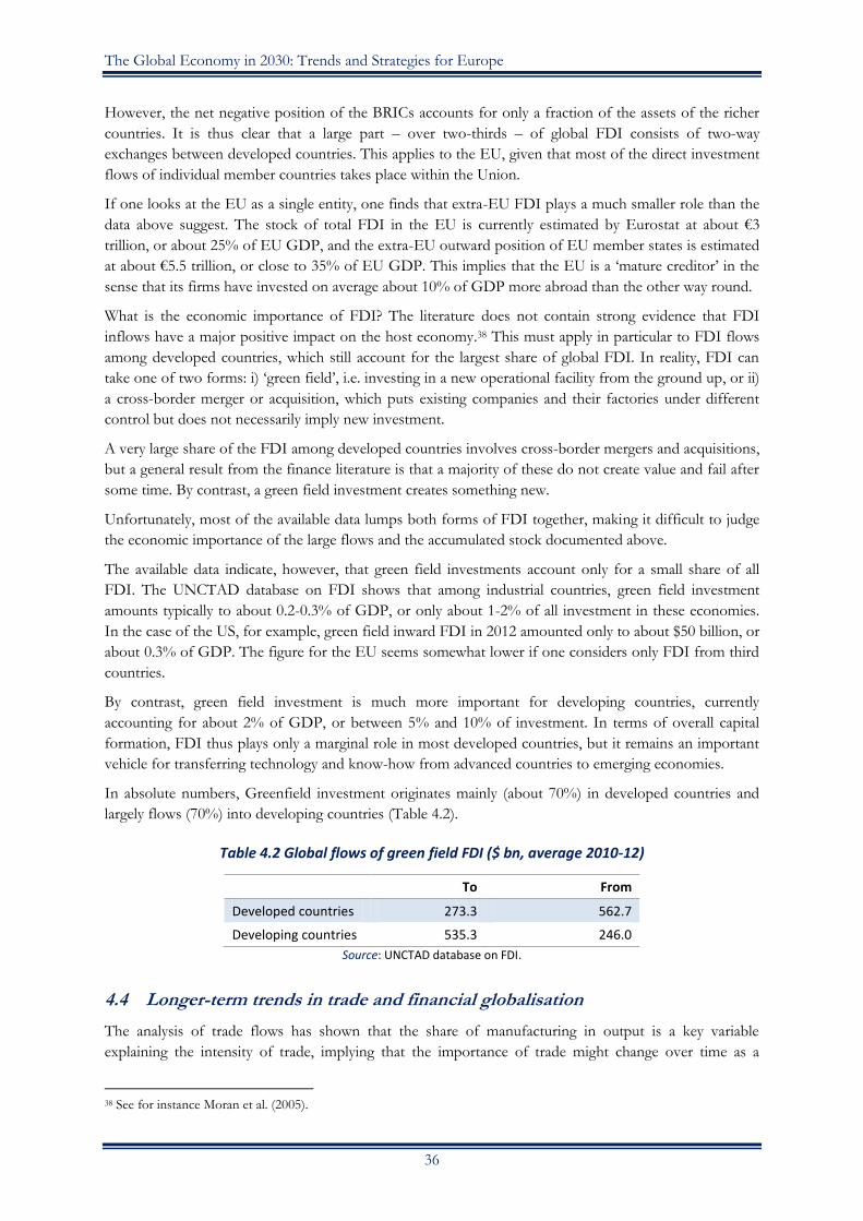
The Global Economy in 2030: Trends and Strategies for Europe
36
However, the net negative position of the BRICs accounts for only a fraction of the assets of the richer
countries. It is thus clear that a large part – over two-thirds – of global FDI consists of two-way
exchanges between developed countries. This applies to the EU, given that most of the direct investment
flows of individual member countries takes place within the Union.
If one looks at the EU as a single entity, one finds that extra-EU FDI plays a much smaller role than the
data above suggest. The stock of total FDI in the EU is currently estimated by Eurostat at about €3
trillion, or about 25% of EU GDP, and the extra-EU outward position of EU member states is estimated
at about €5.5 trillion, or close to 35% of EU GDP. This implies that the EU is a ‘mature creditor’ in the
sense that its firms have invested on average about 10% of GDP more abroad than the other way round.
What is the economic importance of FDI? The literature does not contain strong evidence that FDI
inflows have a major positive impact on the host economy.38 This must apply in particular to FDI flows
among developed countries, which still account for the largest share of global FDI. In reality, FDI can
take one of two forms: i) ‘green field’, i.e. investing in a new operational facility from the ground up, or ii)
a cross-border merger or acquisition, which puts existing companies and their factories under different
control but does not necessarily imply new investment.
A very large share of the FDI among developed countries involves cross-border mergers and acquisitions,
but a general result from the finance literature is that a majority of these do not create value and fail after
some time. By contrast, a green field investment creates something new.
Unfortunately, most of the available data lumps both forms of FDI together, making it difficult to judge
the economic importance of the large flows and the accumulated stock documented above.
The available data indicate, however, that green field investments account only for a small share of all
FDI. The UNCTAD database on FDI shows that among industrial countries, green field investment
amounts typically to about 0.2-0.3% of GDP, or only about 1-2% of all investment in these economies.
In the case of the US, for example, green field inward FDI in 2012 amounted only to about $50 billion, or
about 0.3% of GDP. The figure for the EU seems somewhat lower if one considers only FDI from third
countries.
By contrast, green field investment is much more important for developing countries, currently
accounting for about 2% of GDP, or between 5% and 10% of investment. In terms of overall capital
formation, FDI thus plays only a marginal role in most developed countries, but it remains an important
vehicle for transferring technology and know-how from advanced countries to emerging economies.
In absolute numbers, Greenfield investment originates mainly (about 70%) in developed countries and
largely flows (70%) into developing countries (Table 4.2).
Table 4.2 Global flows of green field FDI ($ bn, average 2010-12)
To From
Developed countries 273.3 562.7
Developing countries 535.3 246.0
Source: UNCTAD database on FDI.
4.4 Longer-term trends in trade and financial globalisation
The analysis of trade flows has shown that the share of manufacturing in output is a key variable
explaining the intensity of trade, implying that the importance of trade might change over time as a
38 See for instance Moran et al. (2005).

Part I. Global Drivers of Growth
37
country develops. From a long-term perspective, the share of manufacturing in total output should follow
a humped shape over the life cycle of an economy. In very poor countries, agriculture dominates and as
income increases, the share of the primary sector falls and that of manufacturing increases. Only at
medium levels of income per capita does the share of manufacturing begin to fall and that of services
begin to dominate. This view can be used to predict future developments of three major developing
regions as global economic actors:
1. China may have reached the peak of the hump in terms of the share of manufacturing (actually,
for China the hump might look more like a Himalayan peak), and manufacturing and trade
should become less important over the next two decades. The MIRAGE model confirms this
prediction and it is consistent with the rebalancing of the country towards domestic
consumption. In this scenario, services become more important than manufacturing and the
growth pattern becomes less trade-intensive.
2. India, whose income per capita is very low, still has to reach the peak of the hump. Until 2030, its
exports should be more dynamic than those of China, but given the low starting point (about
one-tenth that of China today), India in 2030 will still be a far less important trading nation than
China is today.
3. Sub-Saharan Africa (SSA) is at the very early stages of development and should follow, mutatis
mutandis, a path similar to that of India but with a time lag, given that agriculture is still very
important (and also because exports are dominated by natural resources).
Figure 4.11 Trade and financial flows across economic development
Source: Authors’ own elaboration.
This conjecture is captured by the blue hump-shaped line in Figure 4.11, which shows the development
of these major areas, measured by GDP per capita on the horizontal axis.39 The vertical axis measures
trade as a share of GDP, which first rises with growth but then diminishes as the manufacturing sector
becomes less important. By 2030, China is likely to have moved to the right, nearing but not reaching EU
or US GDP per capita. Trade should nevertheless become relatively less important. By contrast, SSA and
India, which both also move to the left, should experience a growth phase during which trade becomes
more important.
39 We assume that the EU GDP per capita level identifies a mature economy.
China (2030)
China (2013) India (2013)
India (2030)
Exports
Financial outflows
GDP capita
SSA (2013) EU, US (2013)
SSA (2030)
Exports/GDP Financial flows/GDP

The Global Economy in 2030: Trends and Strategies for Europe
38
The red line shows the relationship between financial openness and GDP per capita, which is always
sloping upwards and with an increasing slope. This implies that the involvement of China and other
emerging markets in global finance will increase much faster than one would expect from just looking at
GDP growth rates. Emerging markets must thus be expected to play a key role in global financial
markets. This outlook is confirmed by Speller et al. (Bank of England) who find that, by 2030, only 50%
of all external assets will be held by G7 countries – down from more than 80% in 2010 (and about 90%
in 2000).
4.5 Conclusions
There can be little doubt that international trade has expanded enormously in recent decades. One aspect
of this general trend towards globalisation that has attracted particular attention is the emergence of
global value chains, whereby different parts of the production process are performed in different
countries, meaning that the value-added incorporated in a finished product might not necessarily have
been created in the country where the product was finished and then finally exported.
The macroeconomic data on the value-added content of trade, which have only recently become
available, suggest that this phenomenon is important, especially for smaller and emerging economies.
However, for the larger economies (the US, Japan and the EU as a whole), exports still incorporate about
85% to 90% domestic value-added, although this is already lower than the values of over 90% recorded in
1995. It is widely assumed that this trend towards lower domestic value-added in exports will continue,
which would make the GVC phenomenon important even for the larger economies. This is a possibility,
but not a certainty as the most recent data indicate that the GVC has somewhat diminished in importance
in the wake of the global financial crisis and there are reasons to believe that at least offshoring to China
should diminish over time.
Finally, one should bear in mind that cutting up the value chain does not invalidate the classic framework
of comparative advantage according to differences in the capital-labour ratio. If labour-intensive tasks are
‘offshored’ to China, one should consider this inter-industry trade as equivalent to the exchange of
intermediate products with different capital-labour ratios. However, as Chinese wages increase, this
should become less important by 2030.
The implications of the GVC phenomenon are subtle. As exports contain less and less domestic value-
added, the growth of exports per se becomes less relevant for domestic employment and growth, at least
in the longer run. In the short run, however, economies are more interlinked as critical inputs are often
sourced from abroad and these foreign suppliers cannot be replaced quickly. Shocks are thus transmitted
more intensively across countries. Moreover, the increased movement of intermediate products across
borders must be financed, a fact that cannot always be taken for granted, as the financial crisis of 2008
showed. The aftermath of the crisis confirms this pattern – the immediate impact of the shock was global,
hitting trade in particular, and thus the economies that are especially dependent on exports. However, the
fundamental factors driving differences in potential growth were not affected and the differences in
growth rates remained intact once the recovery started. If the GVC phenomenon increases in importance
up to 2030, one should expect a world that is more interconnected, in the sense that local shocks might
have more global repercussions, but the basic determinants of growth will remain local.
Perhaps the most important finding of the research on the value-added incorporated in exports is that a
surprisingly large proportion of exports of manufacturing goods consists of services. For most countries,
manufacturing exports incorporate up to about 40% of the value-added created by services (business
services, transport, etc.). If one adds to this the direct exports of services, the result is that roughly one-
half of all international trade consists in reality of the exchange of services.
This finding implies that productivity in services is a key factor for the competitiveness of nations, even
for the export of goods. One significant and immediate implication for the EU is that the completion of

Part I. Global Drivers of Growth
39
the internal market for services is not only necessary to liberate domestic growth potential, but also to
maintain the competiveness of the European economy on a global scale. Moreover, the extent to which
the European economy can benefit from trade liberalisation, even if it is formally only for goods, depends
to a large extent on the productivity of its services, or at least those services most directly used as inputs
for goods that can be traded (mainly business services).
5. Technology and innovation
Technology represents new ways of doing things and, once mastered, creates lasting change that business
and cultures do not ‘unlearn’. Adopted technology becomes embodied in capital, whether physical or
human, and it allows economies to create more value with less input, in particular less labour input. New
technologies are mostly aimed at saving costs, but they can also improve the quality and user convenience
of the goods and services. At the same time, however, technology is often disruptive, supplanting
previous ways of doing things and rendering old skills and organisational approaches irrelevant.
Besides considerations on improvements in the quality of life and work, in purely economic terms
technological change matters enormously for the creation and distribution of wealth. Following Krugman
(1997), the sources of growth can be classified as ‘perspiration’ and ‘inspiration’.40 ‘Perspiration’ refers to
the standard factors of production, essentially labour combined with physical and human capital, whereas
‘inspiration’ refers to the ability of an economy to generate new products and processes. The relative
importance of perspiration and inspiration changes with the level of development. At low levels of
income per capita, the returns to investment in physical capital and education will be very high; a
minimum level of infrastructure and of education in the work force is a necessary condition for a
manufacturing base. Once this requirement has been fulfilled, other factors become more important in
determining how the accumulated capital can be put to the most productive use. At an intermediate stage
of development, investment in education and new capital accelerate the absorption of existing knowledge.
As an economy gets closer to the technological frontier, however, it must innovate on its own, and
inspiration then becomes the main driver of growth.
5.1 Total factor productivity
Economic theory suggests that R&D combined with human capital (essentially talented and educated
individuals), a systemic approach to innovation and the generation of knowledge spillovers play a key
role in increasing total factor productivity (TFP), which is what brings about technological change.
However, thinking of technology exclusively in terms of TFP can be limiting in the real world. A
generation of economists who were brought up to identify increases in total factor productivity indexes
with ‘technical progress’ has found it quite paradoxical that the wave of innovations based on the
microprocessor and memory chip has apparently failed to elicit a surge of growth in productivity from the
sectors of the US economy that had been investing heavily in electronic data-processing equipment.41
Nowadays, we continue to observe estimates of TFP (which is not an observable variable) that point
towards a decreasing trend in advanced economies. As shown in Table 5.1, Europe’s performance has
been particularly disappointing since 2000, with negative growth rates after 2007 for both the EU27 and
the (now 17) member states of the euro area (EA). The US, which is usually considered a technological
leader, is also on a path of clearly declining TFP growth. Only Japan seems to have been able to contain
the drop.
40 There is widespread agreement among economists about the ultimate sources of growth, but their relative importance is the subject of heated debate. “I Just Ran Four Million Regressions” (Sala-i-Martin, 1997) is a well-known work about the difficulty of understanding the determinants of growth. 41 This ‘productivity paradox’ attained popular currency in the succinct formulation attributed to Robert Solow: “We see the computers everywhere but in the productivity statistics.”

The Global Economy in 2030: Trends and Strategies for Europe
40
Table 5.1 Average annual TFP growth rate (%)
EU27 Euro area US Japan
1995-2000 NA 0.94 1.74 0.41
2000-2007 0.88
0.45 0.80 1.13
2007-2012 -0.54 -0.47 0.63 0.24
2000-2012 0.29
0.07 0.73 0.76
Source: Ameco database, European Commission.
There are several ways to explain this productivity paradox, which are not alternatives to each other, but
rather complementary.42
A first explanation considers the concept of a technological frontier. When an economy approaches this
frontier, it reduces the possibility of importing capital and know-how from abroad and technological
change cannot occur without inputs from education and R&D. According to many experts (e.g.
Acemoglu et al., 2006), Europe had already reached the productivity frontier in the mid-1990s. This
implies that new inputs into innovation and technological change are needed to make good use of its
capabilities to progress further, and this is a particularly challenging task.
A second explanation for the slowdown in TFP relates to the time needed to reap the benefits of
technology. It is argued that general-purpose technologies, which are the ones with the greatest impact on
the economy and society, take time to be diffused and generate growth. Before this happens, a negative
effect is often observed due to the time and investment (including institutional changes and public
acceptance) needed to adapt to the new model. This argument stems from the perspective afforded by the
economic history of the large technical characteristics of network industries; it can be applied, e.g. to
explain the productivity paradox observed in the past with the electrification of factories, stores and
homes, as well as with the recent diffusion of computers and information technologies (David, 1990).
Today, the nature of human interactions with machines and the technical problems of designing efficient
interfaces for humans and computers/smart tools are enormously more subtle and complex than those
that arose from the implementation of electric lighting and power technology. Information has special
attributes that make direct measurement of its production and allocation very difficult and reliance upon
conventional market processes very problematic. Information is different, too, in that it can give rise to
‘overload’, caused by the usually negligible costs of distribution that may encourage information
transmitters to be indiscriminate in broadcasting their output. At the user end, our cultural inheritance
continues to assign high value to (previously scarce) information, predisposing us to try to screen
whatever information becomes available. Screening is costly, however, and the growing duplicative
allocation of human resources to coping with information overload may displace activities producing
commodities that are better recorded by the national income accounts.43
Last but not least – and this is the third way to explain the productivity paradox – the problem could
simply be one of measurement of TFP, also in relation to the lack of adjustment for quality. Firms often
invest in R&D to improve the quality of their products and not the production process. Such changes are
not captured by statistical measurement. Moreover, the deficiencies of the conventional productivity
42 For an explanation, see Hulten (2001). 43 Another important analogy between the diffusion of the electric dynamos and the computers is drawn in David (1990). The information structures of firms (i.e. the type of data they collect and generate, the way they distribute and process it for interpretation) may be seen as direct counterparts of the physical layouts and materials flow patterns of production and transportation systems that had to be changed to enable electrification. In one sense they are, for they constitute a form of sunk costs, and the variable costs of utilising such a structure do not rise significantly as they age. Unlike those conventional structures and equipment stocks, however, information structures per se do not automatically undergo significant physical depreciation. While widespread opportunities to embody best-practice manufacturing applications of electric power awaited the further physical depreciation of durable factory structures, one cannot depend on the mere passage of time to create occasions to radically redesign a firm’s information structures and operating modes. Consequently, there is likely to be a strong inertial component in the evolution of information-intensive production organisations, which hinders the diffusion of new ICT technologies and slows down standard productivity measures.

Part I. Global Drivers of Growth
41
measures are especially problematic in treating the new kinds of products and process applications that
tend to be found for an emergent general-purpose technology during the initial phases of its
development. The problems are i) unmeasured quality changes associated with the introduction of new
commodities and ii) the particular bias of the new technology towards expanding the production of
categories of goods and services that previously were not being recorded in the national income accounts.
Here, too, the story of dynamo revolution holds noteworthy precedents. In the transport sector, for
instance, the contribution to the improvement in economic welfare in the form of shorter journey times
and passenger waiting times afforded by electric streetcars, and later by subways, all remained largely
outside the conventional indexes of real output and productivity.
5.2 Our predictions
Despite the statistical complexities, future estimations about TFP are shown below on the basis of the
MaGE model.44 The model predicts positive and constant TFP growth for advanced economies in the
range of 1-2% up to 2030, and higher but declining rates for China and India (panel b in Figure 5.1).
Figure 5.1 Projections of total factor productivity (1980-2030)
(a) % of US level (b) Growth rates
Source: MaGE estimations and projections.
Despite these higher rates for China and India, advanced economies will maintain their leadership. Japan
will almost completely close the gap with the leader, the US, whereas the EU will continue to lag behind
due to the gap in educational attainment. Emerging economies will continue the process of catching-up
but slowly, given the very low starting point (Figure 5.1, panel a).
Table 5.2 shows that total R&D spending, both private and public, as a percentage of GDP has slightly
increased in all advanced economies during the last two decades. Japan, where the change is more
substantive and largely driven by the private sector, is an exception.
44 The model presents two main determinants of TFP growth. The first is human capital, which is proxied by the share of people of working age in a population who have completed secondary and tertiary education, with tertiary education being important to generate the ‘inspiration’. The other is the distance from the technological frontier, which in practice means the distance from the country with the highest productivity growth, notably the US in recent decades. The greater the distance from the frontier, the higher is the expected TFP growth. It is easier for countries starting at a very low level of development to improve their productivity via the process of imitation than for more advanced economies that need to generate more and more innovation.
0%
10%
20%
30%
40%
50%
60%
70%
80%
90%
100%
1980 1990 2000 2010 2020 2030
US CHN IND JPN EU SSA
-6%
-4%
-2%
0%
2%
4%
6%
8%
1980 1990 2000 2010 2020 2030
US CHN IND JPN EU SSA

The Global Economy in 2030: Trends and Strategies for Europe
42
Table 5.2 R&D intensity, 1995-2011 (% of GDP)
(a) Total economy R&D intensity (b) Business sector R&D intensity
EU27 EA17 US Japan
1995 1.80 1.77 2.48 2.87
2000 1.86 1.84 2.69 3.00
2007 1.85 1.88 2.69 3.46
2009 2.02 2.06 2.87 3.36
2011 2.03 2.09 NA NA
EU27 EA17 US Japan
1995 1.12 1.09 1.75 1.87
2000 1.20 1.18 2.01 2.13
2007 1.18 1.20 1.92 2.70
2009 1.25 1.27 2.02 2.54
2011 1.26 1.31 : :
Source: Eurostat.
The trend towards increased R&D investment is expected to continue in all advanced economies and to
accelerate in China up to the point of challenging the west’s supremacy. Two scenarios can be envisaged:
i) Under the assumption that R&D in the US and the EU rises to 3% of GDP, while in China it
remains constant at the current rate (1.55%), the convergence in absolute terms will be achieved
between the three regions shortly after 2030 (see continuous lines in Figure 5.2).
ii) Under the assumption that R&D expenditure as a share of GDP remains at current levels in
Europe (2.2%) and in the US (2.9%) and rises to 3% in China, by 2030, the effort of the Chinese
economy will be almost double that of the EU and US (see broken lines in Figure 5.2).
Figure 5.2 R&D spending scenarios, 2010-30 (current billion USD)
Source: Authors’ elaboration based on MAGE results.
Under the second scenario, the west’s supremacy in innovation and technological progress could be at
risk by 2030. Of course, R&D spending alone is not a sufficient condition for this to happen; the quality
of such spending and whether it supports educated individuals who can convert research into progress is
of crucial importance. In this respect, there is little doubt that the importance of education has been
acknowledged at the political level. Many countries have set ambitious targets that foresee larger portions
of the younger cohorts in higher education over time, such as the EU202045 strategy for Europe
45 The EU2020 strategy recommends that member states invest at least 3% of GDP in R&D and increase the graduation rates of the 30-34 years cohort to at least 40%.
0
200
400
600
800
1000
1200
2010 2012 2014 2016 2018 2020 2022 2024 2026 2028 2030
US EU
China

Part I. Global Drivers of Growth
43
(European Commission, 2010) and the National Plan for Medium- and Long-Term Education Reform
and Development in China.46
To stimulate innovation and growth, however, it is not sufficient to simply attain a certain amount of
investment in R&D, a certain proportion of university graduates in society or a certain degree of
intangible capital. What matters is the delicate equilibrium between all of these factors and the interaction
between them. Moreover, Aghion (2013a) stresses that innovation-led growth inherently involves a
conflict between the old and the new, and the quality of institutions is not indifferent in this respect. The
conflict is often suppressed in authoritarian regimes, while democracy helps to reduce entry barriers to
innovators. In general, the positive correlation between democracy and innovation/growth tends to be
stronger in economies closer to the technological frontier. The implication of this finding is that by 2030,
China might arrive at the point (of productivity per worker at about 30% of frontier-GDP) where a lack
of democracy results in a serious impediment to growth. While a large part of global GDP today is
produced in countries that are not democracies, no country that is not a democracy has been able to
produce an economy based on innovation.
This implies that what matters for technology and growth is a delicate equilibrium between tangible and
intangible assets, the quantity and the quality of human capital, competent institutions and open societies.
Whether TFP starts growing again will not necessarily depend on single innovations, such as space
technology and cloud computing, but rather on the knowledge mix and the degree of openness of society.
5.3 The impact of breakthrough technologies
Besides being more or less accurately reflected in the evolution of TFP, specific technologies can have
profound impacts on the economy.47 We fail to appreciate that tools invented for a certain purpose in the
past have often become a game changer for other sectors, and this is likely to happen more often thanks
to easier access to information and the Internet. For this reason, it is worth trying to anticipate some new
technologies and innovations that are likely to introduce pervasive changes and improve our quality of life
in the coming years.
Work organisation and new forms of learning. A wide range of educational innovations will occur,
linked to the uptake of new learning platforms, such as mixed reality, pervasive mobile computing,
adaptive learning platforms and gamification. A very promising development is the advent of massive
open online courses (MOOCs) at the university level, which allow for large-scale online participation and
operate via the creation of networks. At the same time, ICT (information and communications
technologies) will also continue to transform work, enabling more agile workflows and reducing costs.
The idea of a fixed physical workplace will change as new technologies allow remote working with
realistic experiences. Yet, it is difficult to predict how long it will take for European citizens to move
towards new forms of learning and to adopt innovative workplace practices on a large scale. There is little
doubt that these practices are beneficial for firms as well as for workers, yet many workplaces in Europe
(in both the private and public sectors) resist change (Beblavý et al., 2012), mostly because of
implementation costs, an unclear regulatory framework or a lack of skills.
Social networks. ‘Web 2.0’, referring to websites that use technology beyond the static pages of earlier
websites, allows people to share content and collaborate online. While members of social networks evolve
from being passive consumers to active producers of content (‘prosumers’), user-generated content will
grow exponentially, creating economic value in a variety of ways. Most of this value is very difficult to
quantify, because it is realised by dispersed communities who do not pay through a monetary price for
membership but rather through the consent given to the service providers to use personal data. To give
an idea of the economic relevance of social networks, the value generated by Facebook in Europe in 2011
46 A paper version of China’s plan is available upon request to the authors. 47 See McKinsey Global Institute (2013) for an overview of the technologies that are expected to have the greatest impact up to 2030.

The Global Economy in 2030: Trends and Strategies for Europe
44
was more than €15 billion, with an average growth of €3 billion a year.48 Social networks also facilitate a
number of applications (apps) in a variety of fields, for instance gaming, recruitment and leisure. Social
networks are also being used in civic contexts to support citizens’ e-Participation, and within public
administration and business ecosystems to improve knowledge-sharing and to streamline decision
processes, as well as to foster co-creation of value and improve productivity.
Internet of Things, big data, automation of knowledge work. It is estimated that by 2015, there will
be 25 billion wireless devices globally and that this number will double to 50 billion by 2020.49 The spread
of sensors (motion and temperature detectors, level indicators, smart meters, etc.) enables the gathering
of huge amounts of data about the real world and the sharing of this data through cloud computing
services. Services around the data value chain are expected to proliferate in the coming decades,
generating new waves of productivity growth and consumer surplus. For example, a retailer using big data
has the potential to increase its operating margin by more than 60%. In the developed economies of
Europe, government administration could save more than €100 billion in operational efficiency
improvements alone by using big data (McKinsey Global Institute, 2011). Amongst several other ways to
create value, big data can be used also to improve the efficiency of infrastructures in the context of smart
cities and wider geographical scopes. For instance, it is estimated that smart grids and smart buildings can
generate about €50 billion in annual energy savings in the EU by 2020. More broadly, a trend towards
enhanced consumer surplus will continue and accelerate across all sectors as they deploy big data. For
example, the use of big data can enable improved health outcomes, higher-quality civic engagement with
government, lower prices due to price transparency and a better match between products and consumer
needs, as companies can leverage data both to design better products and to improve them as they are
used. Automation of knowledge work is another technological frontier. A confluence of advances in
computational speed, machine learning and natural use interfaces has brought computing to an important
milestone: computers are now becoming capable of doing jobs that previously were assumed only
humans could perform (Brynjolfsson & McAfee, 2011).
Cloud computing. Cloud computing is a game-changing innovation that can drastically reduce ICT and
energy costs and enhance the use of digital platforms, content and services. The global cloud computing
market will grow from $40.7 billion in 2011 to over $241 billion in 2020 (Ried & Kisker, 2011). It is
estimated that cloud computing can contribute up to €250 billion to EU GDP in 2020 and could reach a
total cumulative gain of €940 billion for the period 2015-20. The impact on SMEs (small- and medium-
sized enterprises) is expected to be particularly strong, leading to the creation of around 400,000 new
SMEs over a period of five years and permanently shifting the structure of the economy.
Additive manufacturing. Additive manufacturing is a group of technologies that allows a machine to
build an object by adding one layer of material at a time. Additive manufacturing, or ‘3D printing’, is
already in use to make models from plastics in sectors such as consumer products and the automotive and
aerospace industries. In a more or less distant future, additive manufacturing could replace some
conventional mass production, particularly for short production runs or where mass customisation has
high value. Additive manufacturing could also lead to large numbers of micro-factories akin to craft guilds
in the pre-Industrial Revolution era, but with modern manufacturing capabilities. Such local micro-
factories could manufacture significant amounts of products, especially those for which transportation
costs are traditionally high or delivery times are long, and in the process shorten and simplify supply
chains. The developing world could be a major beneficiary because additive manufacturing allows
products to be designed and printed for local consumption, reducing the reliance on expensive imports.
Additive manufacturing could also level the playing field for those countries or organisations that missed
out in previous stages of economic growth because it requires less industrial infrastructure than
conventional manufacturing. However, the key uncertainty in this sphere is the speed of evolution of
such technologies. In their current shape, additive manufacturing techniques have experienced very
limited diffusion and this is most likely to continue to be the case up to 2030.
48 See Deloitte (2012). 49 See Cisco Systems (2011).
Part I. Global Drivers of Growth
45
Resource efficiency. Technology advances will be required to accommodate the increasing demand for
resources owing to global population growth and economic advances in still under-developed countries.
Such advances can affect the food, water and energy nexus by improving agricultural productivity through
a broad range of technologies encompassing precision farming and genetically modified (GM) crops for
food and fuel. New resource technologies can also enhance water management through de-salinisation
and irrigation efficiencies. In addition, they can increase the availability of energy, not only through highly
successful enhanced oil and natural gas extractions resulting from the use of hydraulic fracturing, but also
through alternative energy sources such as solar and wind power, and biofuels.
Healthcare technologies. Disease management technologies in development promise significant
longevity gains throughout the world, while technologies that supplement humans will likely transform
everyday life, particularly for the elderly and mobility-impaired populations. Health technologies (like
specific mobile technology) could prove useful to reduce the expenditure on heathcare. Given the current
burden on public finances and the potential increase in expenditure due to ageing populations,
technologies such as personalised medicine and those that attempt to imitate the functioning of the
human brain could not only increase the productivity of the sector which, being a non-tradable one, is not
bound by international competition, but can also generate savings.
5.4 Advanced technologies will not destroy jobs
All the innovations presented above, and several others, will come together to create a new technological
regime that promises to make the ‘information overload’ problem less dramatic. Most of the knowledge
produced could be processed automatically by smart devices or by humans, assisted by knowledge work
automation tools and systems. The automation of knowledge work could bring great societal benefits –
such as improved quality of healthcare and faster drug discovery – but it may also spark complex societal
challenges, particularly in employment and the education and retraining of workers.
Indeed, it is not surprising that new technologies make certain forms of human labour unnecessary or
economically uncompetitive and create demand for new skills. This has been a common phenomenon
since the Industrial Revolution – the mechanical loom marginalised home-weaving while creating jobs for
mill workers. But this time the impact of the ‘great transformation’ promises to be different, because
today’s displaced industrial workers cannot simply move into knowledge work or services the way
displaced farmers and domestic workers moved into industrial work in the 19th and 20th centuries. The
extent to which today’s emerging technologies could affect the nature of work is unprecedented.
Automated knowledge work tools will almost certainly extend the powers of many types of workers and
help drive top-line improvements with innovations and better decision-making, but they could also
automate some jobs entirely. Advanced robotics could make more manual tasks subject to automation,
including services where automation has had little impact until now. At the very least, the benefits of new
disrupting technologies may not be evenly distributed, and could even contribute to widening income
inequality. Advanced technology, such as automation of knowledge work or advanced robotics, could
create disproportionate opportunities for some highly skilled workers and owners of capital while
replacing the labour of some less-skilled workers with machines. Recently, Brynjolfsson & McAfee (2011)
put forward the argument that technology is more radically displacing jobs in the US economy than ever
before:
The pattern is clear: as businesses generated more value from their workers, the country as a
whole became richer, which fuelled more economic activity and created even more jobs. Then,
beginning in 2000, the lines diverge; productivity continues to rise robustly, but employment
suddenly wilts. By 2011, a significant gap appears between the two lines, showing economic
growth with no parallel increase in job creation.
However, the reality is that there is no logical relationship between job growth and productivity. To see
why, imagine two nations with annual productivity growth of around 2%. Nation A has a declining
workforce because more people are retiring than are reaching prime working age. Nation B has a growing
workforce because of higher fertility rates among workers and immigration. As this example of real
nations shows – Japan as nation A and the US as nation B – an economy can have high productivity and

The Global Economy in 2030: Trends and Strategies for Europe
46
low or high employment growth. So, the reason why job growth slowed after 2000 was largely
demographic. The number of adults in the workforce (employed and unemployed) grew by 18% in the
1980s, 13% in the 1990s but just 8% in the 2000s as baby boomers got older and women’s entrance into
the workforce peaked (Atkinson, 2013).
Brynjolfsson and McAfee’s argument is wrong as it considers only first-order effects of automation where
the machine replaces the worker. But when a machine replaces a worker, there is a second-order effect:
the organisation using the machine saves money and that money flows back into the economy either
through lower prices, higher wages for the remaining workers or higher profits. In all three cases, the
money gets spent, which stimulates demand that other companies respond to by hiring more workers.
This common-sense view is borne out by almost all economic studies looking at the relationship between
productivity and jobs. While some studies have found that productivity growth does have some short-
term negative job impacts, all the studies find either no impact or a positive impact on total jobs in the
longer term.
Economic theory and government policy will have to be rethought if technology is indeed destroying jobs
faster than it is creating new ones. But technologies like the internet, artificial intelligence, big data and
improved analytics – all made possible by the ever-increasing availability of cheap computing power and
storage capacity – that are automating many routine tasks will not necessarily kill human jobs at an
unprecedented rate. First, because to do so, productivity growth rates should increase significantly, but
there is little evidence that productivity can grow in excess of 3% a year. This is in part because despite IT
advances that boost productivity in information-based functions, a growing share of jobs involves
interacting with people (e.g. nursing homes, police and fire services) or doing physical tasks that are
difficult to automate (e.g. construction or janitorial services). Second, even if the rate of productivity
miraculously increases to, say, over 5% per year, it still does not matter for jobs. For that would mean that
national income increases by 5% per year and we would all buy more meals in restaurants, holidays, cars,
houses, therapeutic massages, college educations, 3-D TVs, and so on. Workers have to produce these
goods and services, and if these are somehow automated, then we have even more money to spend and
would buy other goods and services, creating jobs in these functions.50
The reality is that, since the first Industrial Revolution, labour-saving productivity improvements have
been made at an unprecedented rate in most manufacturing activities, reducing the cost of making these
products, even as workers’ wages have risen. Meanwhile, in other sectors of the economy, notably in the
personal services industries, automation is hardly possible, and labour-saving productivity improvements
occur at a rate well below average for the economy. As a consequence, it is difficult to reduce the quantity
of labour required to produce these services, at least without reducing the quantity of services delivered at
a standard quality level. This stems from the nature of ‘personal services’, which usually require direct,
face-to-face interaction between those who provide the service and those who consume it.
Yet, despite no measurable productivity achievement, the price of these services continues to grow. This
phenomenon, known as the ‘Baumol cost disease’, asserts that the costs of healthcare, education, live
performing arts and a number of other economic activities known as ‘personal services’ are condemned
to rise at a rate significantly greater than the economy’s rate of inflation. The reason is not difficult to
identify: the items in the rising-cost group – the stagnant sector – generally have a human element not
readily replaceable by machines in their production process, which makes it difficult to reduce their labour
content. Items whose costs are falling – the progressive sector – are predominantly manufactured via
more easily automated processes. Their steadily falling real costs simply reflect their declining labour
content. According to Baumol (2012), it is possible to turn the cost disease into an opportunity for future
development of modern economies beyond the conventional GDP-based growth model. The key is to
make sure that the unprecedented productivity growth continues at the global level in the future, for this
will ensure that both wages and per capita income will continue to rise, making most products and
services cheaper relative to consumers’ buying power. This means that we can afford not merely the
50 This argument obviously holds for well-functioning democratic economies, where the benefits of technological change are widely distributed within the whole society and are not concentrated in the hands of a few affluent people and autocrats.

Part I. Global Drivers of Growth
47
survival of the stagnant services, but also ever-greater quantities and rising quality in the future, despite
their rising costs. One must understand that the source of the problem, paradoxically, is the growth of
our economy’s labour productivity – or rather the unevenness of that growth – boosted by labour-saving
technological innovation in the progressive (industry and service) sectors. This creates the problem, but
also the potential solution, provided that we become aware of the cost-disease paradox and its
implications.
In this puzzle, technological and social innovation should act as unified forces and drivers of change. The
former should boost labour productivity and produce more and better products while saving/freeing
labour in the progressive sectors of the economy, while the latter aims to enhance the quality of
environment, health, education and other personal care and social services provided to the population,
while creating new jobs in these typically labour-intensive activities (where new technologies are used
mostly to provide more quality to users – for example, through advanced healthcare technologies – rather
than reducing labour input). Together with policies to boost productivity, there will be the need to
examine systematically, for the stagnant sectors, two questions: i) What outputs cost to produce and
consequently what consumers (private or public) must pay to purchase them? ii) Which benefits will
accrue to the consumers – that is, how good is the product for the money that consumers spend? For the
latter point, it is important to note that as the stagnant services produce mostly intangibles (health and
well-being, education and knowledge, aesthetic values, etc.), the standard output measures in terms of
GDP are not appropriate to fully measure the impacts of innovation and quality improvements. In
addition to GDP measures of standard of living, we therefore need metrics that account for true value.
6. Natural resources: Energy and metals
Economic growth will remain the key driver behind an increasing demand for natural resources, especially
in Asia. However, at least until 2030, the supply of fossil fuels, minerals, metals and biomass is likely to
keep up with demand. Possible exceptions include critical metals such as rare earths, which are at risk of
supply shortage with potentially negative impacts on the economy. But increasing European production
of these critical resources, better waste management, recycling and substitution with more common
materials can help to secure supplies and keep prices down. The key challenge for the EU and the rest of
the world will therefore not be the availability of natural resources, but their price and the negative
environmental effects associated with their extraction, use and emissions.
The control, extraction and use of natural resources has been present throughout human history.
Recently, however, the demand for natural resources has accelerated to the extent that it is now a major
driver of environmental problems such as climate change, biodiversity loss, desertification and ecosystem
degradation. Over the past three decades, the global extraction of metals, fossil fuels, minerals and
biomass has increased from below 40 billion tonnes in 1980 to almost 70 billion tonnes in 2008. This
represents an increase of some 80%, or about 2.1% per year (SERI, 2011). Extraction rates are expected
to accelerate further over the next two decades. In a business-as-usual scenario, i.e. without any additional
policy measures to increase resource efficiency or decrease resource use, the annual rate of resource
extraction will increase to 2.5% between 2010 and 2030, resulting in an absolute global (used) extraction
of natural resources of over 100 billion tonnes in 2030 (SERI, 2011). This acceleration of resource
extraction is linked to the rapid rise of new consumer classes in emerging economies, where people aspire
to lifestyles comparable to those in industrialised countries.
The medium-term trend is thus towards a more rapid rate of resources use, but the long-term outlook
suggests the very opposite. Resource use might stabilise sometime after 2030 because the world’s
population is likely to stabilise then. The long-run demographic trends thus push in the opposite direction
of the short- to medium-run economic trends.
Concerns that the supply of natural resources is nearing exhaustion are not new. The most widely used
model of the pricing of natural resources (Hotelling’s rule) was actually inspired by this concern:

The Global Economy in 2030: Trends and Strategies for Europe
48
Contemplation of the world’s disappearing supplies of minerals, forests, and other exhaustible
assets had led to demands for regulation of their exploitation. The feeling that these products are
now too cheap for the good of future generations, that they are being selfishly exploited at too
rapid a rate, and that in consequence of their excessive cheapness they are being produced and
consumed wastefully has given rise to the conservation movement.
These words constitute the introduction to Hotelling’s seminal scientific paper of 1931!
The model proposed by Hotelling was designed to elucidate how to use the resources already found. But
the key issue for the long-term future is not so much how to use the reserves already known, but whether
the rate of discovery of new reserves will continue to increase at a similar pace as in the past. This in turn
depends on the rate at which the cost of extraction increases as ever-more remote regions are prospected
and ever-more difficult geological formations must be mastered. The development of offshore oil and gas
production shows that incremental technological progress can continuously make additional reserves
accessible, albeit at an increasing cost. And the example of the ‘shale gas revolution’ shows that
technological progress can sometimes even lower the cost of accessing reserves, which previously were
unknown or thought to be inaccessible.
From an economic point of view, the key issue is how rapidly the cost of extraction increases and thereby
necessitates higher prices. The run-up in raw-material prices over the past decade has fuelled the
impression that that ‘this time is different’ in that the limits have been reached. A recently published data
set on very long-term price trends shows that the perception of whether prices tend to increase is strongly
determined by the length of the period under consideration (Jacks, 2013).
Importantly, the long-term trends for the prices of reproducible goods, i.e. ‘commodities to be grown’
and exhaustible resources i.e. ‘commodities in the ground’ seem to differ fundamentally. The real price of
the former has actually trended downwards over the last century, whereas the commodities in the ground
(those that cannot be reproduced) have seen large swings and now appear, as diagrammed in Figure 6.1,
to be close to the peak of a ‘super cycle’.
Figure 6.1 Real commodity prices in the very long run, 1900-2010 (1900=100)
Source: Jacks (2013).
At the most basic level, the concern about the availability of natural resources is based on the argument
that an ever-increasing population will generate an ever-increasing demand for resources that must sooner
or later be exhausted. The observation that by 2030 the growth of the global population will probably
have come to an end (or that the end might be in sight) will have a profound implication: the end of the
growth of the demand for resources might then also be in sight. It is clear that by 2030 the demand for
material resources will continue to grow, given that large parts of the world will still have a much lower
per capita consumption rate than the richest ones. But this will be temporary. A ceiling should be reached
when most of the world’s population has caught up with the leader in terms of technology and standard

Part I. Global Drivers of Growth
49
of living. That ‘ceiling’ is still far from being reached. The material consumption per capita in Europe
today is around 20 tonnes; about twice the world average of 10 tonnes. This implies that global resources
consumption of all commodities would increase by about 100%, from somewhat above 70 billion tonnes
to 160-170 billion tonnes annually – if the entire world were to achieve European levels (of material
consumption). But it could well stabilise from that point onwards.
Figure 6.2 shows global total material consumption under the assumption that the entire world will
achieve European levels by 2050 and that after that point material consumption per capita will continue
to increase, but at a much slower rate because the whole world will then have a mature economy. Under
the low population variant (which we hold most likely), these assumptions imply that global material
consumption could stabilise by around 2050 and perhaps even decline slightly, even if economic growth
continues. By contrast, under the high population variant (which corresponds roughly to an extrapolation
of past population growth rates), material consumption would never stabilise.
Figure 6.2 Two scenarios for resource use (billions of metric tonnes per year)
Data source: Authors’ own calculations based on UN population data and F. Krausmann, S. Gingrich, N. Eisenmenger,
K.H. Erb, H. Haberl and M. Fischer-Kowalski, “Growth in global materials use, GDP and population during the 20th
century”, Ecological Economics 2009.
All in all, material consumption is a function of three variables – population growth, prosperity and
technology – the first two of which tend to increase the use of resources and the latter with an ambiguous
effect. Between now and 2030, because of rapid output growth, resources consumption is likely to
increase and to converge towards current European levels (around 20 tonnes per capita). But conceptually
the situation changes fundamentally once population growth has ended. From that point onwards, the
demand for material resources grows only with income and once the global average income level has
converged to that of today’s leading economies, material consumption should grow only if technological
progress is biased against resource savings. General increases in productivity should lead to higher income
per capita, which increases the demand for material resources, but the increase in productivity should also
reduce the need for material inputs per unit of GDP. If technological progress is not biased, the two
forces should approximately cancel each other out.
The key argument about resource availability is thus no longer that a never-ending growth of material use
must sooner or later reach the limit of resource availability, but rather whether a rate of resource
extraction of approximately twice today’s level is sustainable. Given the long history of failed predictions
about the supply of natural resources being about to run out, we believe that the problem will not be
‘below ground’ in the sense that this rate of resource extraction will not lead to acute scarcities, at least
not in a 2030 perspective. However, there might be problems ‘above ground’, in particular with the global
climate, as discussed in more detail below.
0
50
100
150
200
250
300
350
400
450
20
15
20
20
20
25
20
30
20
35
20
40
20
45
20
50
20
55
20
60
20
65
20
70
20
75
20
80
20
85
20
90
20
95
21
00
High population growth Low population growth

The Global Economy in 2030: Trends and Strategies for Europe
50
The ‘carbon budget’ of the earth, i.e. the amount of CO2 from fossil fuels that can be released into the
atmosphere, might actually be more constraining than the known reserves of fossil fuels. The problem in
this case is thus not resource scarcity, but the use of the vast amount of resources that we know today will
lead to a potentially devastating and unprecedented rise in global temperatures.
6.1 Energy
Europe will feel the environmental effects of the global expansion in material use, probably both in the
form of climate change and price swings in the raw materials that Europe needs for its economy. But
resource scarcity per se seems less of an issue, certainly before 2030. For example, the reserves-to-
production ratios of oil, gas and coal are just over 50, 60 and 100 years, respectively (BP, 2012). This
means that there are enough known reserves to meet global demand, at least until the 2060s (at current
production levels). However, the use of carbon-intensive fossil fuels, and in particular of coal, might be
subject to carbon pricing, which should lead to rising fossil fuel prices relative to low-carbon fuels, such
as natural gas.51
Relative price changes and policy measures are likely to underpin an ever-increasing share of renewables
in world primary energy demand, which is projected to grow from 13% in 2010 to almost 17% in 2030
(IEA, 2012).
The trend towards renewables will also have an impact on the demand for metals, especially for high-tech
metals that are crucial for EU high-tech and eco-industries in energy (e.g. for wind turbines, solar panels
and energy-efficient light bulbs), transport (e.g. electric car batteries) and electronics manufacturing (e.g.
computers). In fact, the transition to a low-carbon economy as planned for the EU depends to a large
extent on these resources.
6.2 Metals
While the EU is self-sufficient in construction minerals and a major producer of industrial minerals, it is
highly dependent on imports of high-tech metals (European Commission, 2008). In terms of primary rare
earths, for example, the EU has no domestic production activities at all and is thus entirely dependent on
imports (European Commission, 2013a). Supply risks stem from the fact that production is concentrated
in a few countries, while substitution and recycling rates are low. Although supply is likely to adjust over
time, there may be temporary bottlenecks causing price hikes and supply disruptions with potential
negative effects on European industry and economic performance.
The Joint Research Centre (JRC) (2011) has undertaken a risk analysis for metals required for the
technologies contained in the SET-Plan – nuclear, solar, wind, bioenergy, carbon capture and storage
(CCS) and electricity grids. Its study shows that 14 out of the 60 metals analysed face supply risks in the
short- to-medium term (i.e. over the next five to ten years). These critical metals include dysprosium,
tellurium, gallium, indium, niobium, neodymium, vanadium, tin, selenium, silver, molybdenum, hafnium,
nickel and cadmium. Five of these metals were assessed as having high overall supply risks, including the
two rare earths dysprosium and tellurium, as well as three by-products from the processing of the other
metals tellurium, gallium and indium. In fact, the risk level of the two rare earths has also been validated
by the huge swings in their prices, with an increase of 535% and 385%, respectively, between 2010 and
2011.
51 Another important development that will intensify by 2030 is the increasing intersection of food, water and energy, with much scope for negative trade-offs. For example, agriculture is highly dependent on the accessibility of adequate sources of water as well as on energy-rich fertilisers. Hydropower is a significant source of energy for some regions while new sources of energy – such as biofuels – further threaten the availability of food shortages. In addition, economic growth in developing countries will continue to lead to greater demands for a meat-based diet, putting further pressure on grain markets and water resources. Given the limited availability of new agricultural land, improving crop efficiency will become especially important in meeting global food needs.

Part I. Global Drivers of Growth
51
For all the metals, the largest risk factors are rapid demand growth and political risks, followed by supply
concentration and limits to production expansion.
In dealing with these risks, the EU is best advised to follow a multi-pronged strategy, which includes
energy and resource efficiency, increasing domestic production of critical resources where possible, better
waste management and recycling, as well as the substitution of these resources with more common
materials. This requires action from various policy areas and related Directorates General from the
European Commission (e.g. Trade, Enterprise, Energy, Climate change, Environment, Transportation,
Research, Technology & Development, etc.). The European Innovation Partnership (EIP) is an example
of a broad initiative involving various European Commission departments, aimed at making “Europe a
world leader in raw materials exploration, extraction, processing, recycling and substitution by 2020”
(European Commission, 2013b).
6.3 Water
Access to fresh water in sufficient quantity and quality is becoming a major challenge almost everywhere,
as a result of population growth, urbanisation, wasteful consumption, pollution and climate change.
Accordingly, the achievements under the Millennium Development Goals (MDGs)52 now seem
threatened. According to the UN, 1.2 billion people live in countries with physical water scarcity, and
growing water stress could soon affect a further 500 million people. In addition to physical water scarcity,
1.6 billion people are facing an economic water shortage and lack the means for adequate access.53
The situation is expected to worsen: the FAO has estimated that by 2025, 1.9 billion people will be living
in countries suffering from ‘absolute water scarcity’.54 Population growth will affect the demand for food,
and thus irrigation, as well as water for industry. In poorer countries where many people depend on semi-
subsistence agriculture, access to water is vital.
Climate change is expected to cause and aggravate the virulence of water-related extreme events – both
droughts and floods – with the ensuing socio-economic disruptions (IPCC, 2007d; World Bank, 2013b).
The IPCC 4th Assessment Report (2007d) estimates that by 2020 yields from rain-dependent agriculture
could decrease by 50% due to climate change, which would mean that the share of irrigated land would
need to increase very significantly.
The underlying global trend is that over the last century water demand outstripped population growth by
two.55 Moreover, higher income usually also leads to higher water consumption.
Need for water for food production and energy
The availability of water is obviously a major pre-condition for any increase in food production. The
FAO (2012) estimates that the world’s growing population will require about 50% more food by 2030
compared to 1998.56 This will require increased irrigation. Water for irrigation and food production
already accounts for an estimated 70% of freshwater withdrawal globally, and constitutes one of the
greatest pressures on water resources. In some emerging economies, such as China, water withdrawal for
agriculture can reach as much as 90%, according to the 2012 UN World Water Development Report
52 The Millennium Development Goals (MDGs) include a specific target (No 7c) for water and sanitation, which is to halve by 2015 (based on 1990 levels) the proportion of people without sustainable access to safe drinking water and basic sanitation. While the drinking water objective has been achieved, the sanitation objective has not. 53 World Water Development Report 4. World Water Assessment Programme (WWAP), March 2012. 54 FAO Hot issues: Water scarcity (www.fao.org/nr/water/issues/scarcity.html); The UN defines "water scarcity" as water supply levels below 1,000 cubic metres per person per year, and “absolute water scarcity” as levels below 500 cubic meters. 55 See http://ec.europa.eu/europeaid/what/environment/water-energy/.
56 In the last 30 years, food production has increased by more than 100%.

The Global Economy in 2030: Trends and Strategies for Europe
52
(WWDR).57 Even countries that were traditionally rich in water (e.g. those in northern Europe)
increasingly rely on irrigation due to recurring episodes of drought (Egenhofer et al., 2012).
Ensuring a reliable supply for agriculture requires huge public-sector investments, which today are rarely
in place, thus rendering poorer countries vulnerable to the negative effects of longer dry spells. However,
given that investment rates are generally not much higher in emerging economies than in developed
countries, one can expect that by 2030 most countries should have the necessary infrastructure in place to
ensure that crops no longer fail because of a drought.
In 2012, over 1 billion people lacked access to electricity and other sources of energy. Meeting these
needs will require a surge in energy production, especially in non-OECD countries (UNESCO, 2012).
Energy in general and electricity in particular require water for various production processes (e.g.
extraction of raw materials, cooling processes, cleaning, powering turbines and irrigation for biofuel
crops). Globally, energy presently accounts for 15% of total freshwater withdrawal. In the EU, i.e. in
developed countries, this share is over 40%.58 This suggests that the rapid pace of industrialisation across
emerging economies will lead to a huge increase in water demand. It should be noted, however, that a
large part (sometimes one-half) of the water abstracted for energy production is returned, although
sometimes causing environmental impacts, by affecting the physical and chemical properties of the water.
The net demand for water through the quickly growing energy sector should thus be manageable.
Water demand and supply
It is generally acknowledged that there is significant scope for technological improvement and better
water management. The latter holds high potential: typically, water pricing is applied only to households
and covers only the costs of the water supply network, barely covering the full capital costs, even in the
EU. The source, i.e. water, is normally not priced at all (throughout the EU and globally). Even in the
EU, water use for agriculture is often not even measured, let alone priced. In many emerging economies
this is also the case, even if water is officially scarce. The agricultural sector thus suffers from poor
infrastructure, waste and overconsumption (Egenhofer et al., 2012). The appropriate policy response
would be adequate metering and pricing.
From an economic point of view, warnings of impending water scarcity do not take into account that
both the supply and demand of water should react to the price. This is the key issue since even in dry
regions there is usually enough rainfall, on average, to satisfy a huge demand.
The main areas where water shortages are predicted are in the poorer and less dynamic, emerging
economies where there is usually no water metering, let alone pricing.
Official statistics imply that 90% of water extraction in China is for food production. This probably
means that there is no price. Even a modest price could have a substantial impact since water usage does
respond to price signals, even in agriculture. The experience with irrigation districts in Spain indicates that
a price of 0.1 to .015 euro per cubic meter can lead to a reduction in water usage by one-half.
It is unlikely that water scarcity will be a major economic factor in 2030. As population growth comes to a
halt, already one factor driving the growth of water consumption will slowly disappear. However, demand
for water is still likely to increase as incomes increase and the two major users of water increase their
demand, namely food production and energy. As water scarcity increases, governments will need to
address this either through pricing (including the source) or regulation (including rationing). Given the
57 UNESCO (2012). 58 The structure of water consumption in the EU is dominated by the energy sector (45%), agriculture (25%) and households (20%).
The few available studies suggest that for France the cost of collecting rain water (in a new plant!) is 13% of the price from water from the tap, the cost of recycling treated industrial water is 37% percent of the price of tap water. The water price per cubic meter in France is around €1.00 (for tap water delivered to households); this would imply costs in the order of €0.13 to €0.37 per cubic meter.

Part I. Global Drivers of Growth
53
high price elasticity of water, once pricing (explicit or implicit) is gradually introduced, water will be used
far more efficiently with very significant technological improvements.
Water and crises and the prospect of war?
Due to their trans-boundary nature, water basins and aquifers59 tend to be shared between countries.
Increasing water scarcity is often seen as an important source of conflict.60 Historically, however, water
scarcity has led to increased cooperation rather than conflict (see review of global conflicts and
agreements in international river basins in Stucki, 2005).. Most of the conflicts over the perceived
excessive use of upstream nations should be manageable if one looks only at their economic impact. For
example, the annual average flow of water through the Euphrates at the Turkish border with Iraq varies
between 15 and 45 billion cubic meters.61 In the conflict between Iraq and Turkey, the Iraqi side claimed
that it had been deprived of about 10 billion cubic meters annually. Applying a price of around €0.1/bcm
to this water, which seems appropriate since it would be untreated and suitable mainly for agriculture,
would imply a dispute worth about €1 billion. This must be seen in comparison to two economies whose
annual GDP is worth about €150 billion for Iraq and over €700 billion for Turkey. This dispute, which is
a key example of cross-border tensions over water is thus not primarily about the economic impact of a
higher availability of water.
6.4 The predictions of the model
The MaGE model also has a resource-use component. In the central scenario, the global trend towards
greater resource use continues, but with a different intensity and speed in the developed and the emerging
economies. At the global level, the extraction of economically used resources is expected to continue at a
relatively constant pace until 2030. However, the absolute increase is expected to be higher and is
projected to increase further after 2030. It remains to be seen whether the continuing growth in the use of
exhaustible resources will lead to scarcities and/or price increases. Both would of course have a negative
feedback on growth.
Figure 6.3 Energy productivity (2005, USD per barrel)
Source: MaGE estimations and projections.
59 For a map of trans-boundary aquifers, see Wolf et al. (1999). 60 For a list of water-related conflicts, visit the website of World Water (www.worldwater.org/conflict/list/). 61 See http://en.wikipedia.org/wiki/Euphrates.
0
500
1000
1500
2000
2500
1980 1985 1990 1995 2000 2005 2010 2015 2020 2025 2030
US CHN IND JPN EU SSA
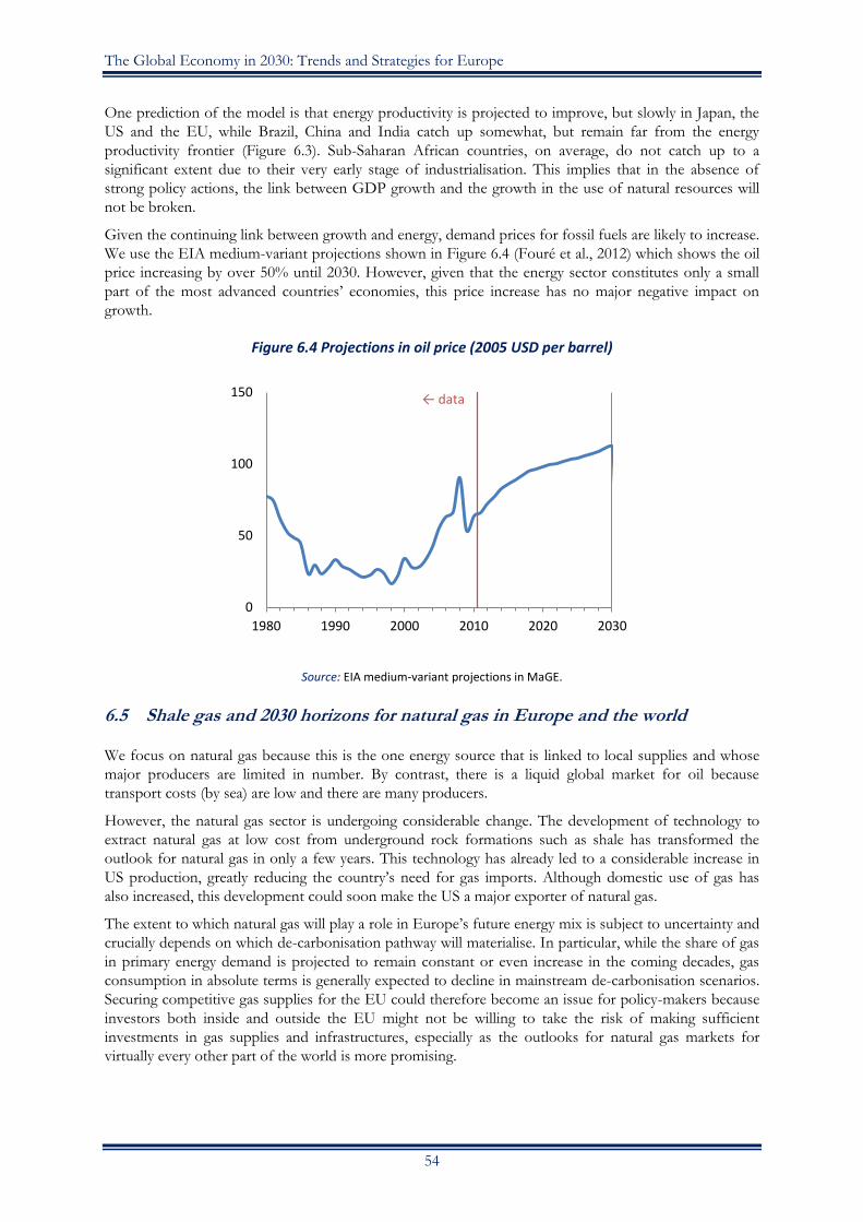
The Global Economy in 2030: Trends and Strategies for Europe
54
One prediction of the model is that energy productivity is projected to improve, but slowly in Japan, the
US and the EU, while Brazil, China and India catch up somewhat, but remain far from the energy
productivity frontier (Figure 6.3). Sub-Saharan African countries, on average, do not catch up to a
significant extent due to their very early stage of industrialisation. This implies that in the absence of
strong policy actions, the link between GDP growth and the growth in the use of natural resources will
not be broken.
Given the continuing link between growth and energy, demand prices for fossil fuels are likely to increase.
We use the EIA medium-variant projections shown in Figure 6.4 (Fouré et al., 2012) which shows the oil
price increasing by over 50% until 2030. However, given that the energy sector constitutes only a small
part of the most advanced countries’ economies, this price increase has no major negative impact on
growth.
Figure 6.4 Projections in oil price (2005 USD per barrel)
Source: EIA medium-variant projections in MaGE.
6.5 Shale gas and 2030 horizons for natural gas in Europe and the world
We focus on natural gas because this is the one energy source that is linked to local supplies and whose
major producers are limited in number. By contrast, there is a liquid global market for oil because
transport costs (by sea) are low and there are many producers.
However, the natural gas sector is undergoing considerable change. The development of technology to
extract natural gas at low cost from underground rock formations such as shale has transformed the
outlook for natural gas in only a few years. This technology has already led to a considerable increase in
US production, greatly reducing the country’s need for gas imports. Although domestic use of gas has
also increased, this development could soon make the US a major exporter of natural gas.
The extent to which natural gas will play a role in Europe’s future energy mix is subject to uncertainty and
crucially depends on which de-carbonisation pathway will materialise. In particular, while the share of gas
in primary energy demand is projected to remain constant or even increase in the coming decades, gas
consumption in absolute terms is generally expected to decline in mainstream de-carbonisation scenarios.
Securing competitive gas supplies for the EU could therefore become an issue for policy-makers because
investors both inside and outside the EU might not be willing to take the risk of making sufficient
investments in gas supplies and infrastructures, especially as the outlooks for natural gas markets for
virtually every other part of the world is more promising.
← data
0
50
100
150
1980 1990 2000 2010 2020 2030

Part I. Global Drivers of Growth
55
The status quo
Natural gas plays a major role in the world’s energy supply, representing some 22% of world energy
demand. It is the second-biggest commodity market in the world (after oil) by value of production (over
$1 trillion in 2011).62 While sectoral gas use varies by region, power generation is generally the largest
consumer of natural gas. But natural gas is also used in buildings (mainly for space and water heating), in
industry (e.g. steel, glass, paper, fabrics and brick), in energy sectors other than power generation (oil and
gas industry operations), for non-energy use as a raw material (e.g. paints, fertilisers and plastics) as well as
in transport (natural gas vehicles). The price of natural gas, therefore, does have a significant impact on
various sectors of the economy.
Figure 6.5 Natural gas prices in the US, Europe and Japan, 1993-2012
Source: World Bank commodity price data.
At present there is no such thing as a global price for natural gas.63 In fact, there are high price
differentials between regions stemming from the relatively high transport and storage costs (compared to
oil, for example). Figure 6.6 shows natural gas price developments from 1993 to 2012, in comparison with
the oil price. From the 1990s to 2007-08, prices for natural gas in the US, the EU and Japanese were
increasing almost in parallel, and also in line with the oil price.64 But as a result of the unexpected shale
gas revolution in the US, American natural gas prices have since fallen to 1990 levels65 – decoupling from
the oil price. In Europe, by contrast, gas prices are now three to four times as high as in the US (departing
from US prices as of 2009), and are not yet fully decoupled from the oil price. Japanese LNG import
prices are even higher than in Europe and still linked to the oil price.
Looking ahead towards 2030
Technically, recoverable natural gas resources seem to be abundant. According to IEA estimates, at 2011
levels of gas consumption, these resources would meet world gas demand for some 230 years. Eastern
62 See Valiante (2013). 63 As a consequence, each region has one or several price benchmarks that are only partly linked to one another. For North America, Henry-Hub (a distribution hub located in Louisiana) prices are generally taken as a benchmark. When talking about European gas prices, one usually distinguishes at least between BAFA CFI (average German border import prices as reported by BAFA - Federal Office of Economics and Export Control) and NBP (National Balancing Point: the British virtual gas hub operated by TSO National Grid, covering all entry and exit points in mainland Britain. For Asia, Platt’s JKM (Japan Korea Marker) may serve as a proxy. 64 As prices are reported in nominal US dollars, the general increasing trend is partly due to inflation. 65 Note that these figures are in nominal terms, and thus in real terms, US gas prices are even lower than 20 years ago.
0
20
40
60
80
100
120
0
2
4
6
8
10
12
14
16
18
19
93
19
94
19
95
19
96
19
97
19
98
19
99
20
00
20
01
20
02
20
03
20
04
20
05
20
06
20
07
20
08
20
09
20
10
20
11
20
12
Cru
de
oil
in n
om
inal
$/b
bl
Nat
ura
l gas
in n
om
inal
$/m
mb
tu
Natural gas, US Natural gas, Europe
Liquefied natural gas, Japan Crude oil, average

The Global Economy in 2030: Trends and Strategies for Europe
56
Europe/Eurasia (mainly Russia) and the Middle East together hold 58% of the remaining (technically
recoverable) conventional gas resources, but only 17% of the remaining unconventional gas resources.
So-called ‘unconventional resources’ have radically changed the picture, mainly in the US (shale gas),
Canada and Australia (coal bed methane), but in the future potentially also in China (huge potential shale
gas resources) and India. Europe also has some shale gas resources (e.g. in Poland, the UK and Ukraine),
but it remains to be seen to what extent their extraction will be commercially (and environmentally)
viable.
The fall in the cost of transporting LNG (liquefied natural gas) by sea represents another important
development as it creates a global market and global gas price linkages. This trend may continue as
traditional regional gas markets are being increasingly globalised. As a result, Europe will have more
choice in attracting competitive gas supplies. Against this background, while the world might be entering
a golden age of gas,66 the EU may be drifting along a different course. In several mainstream
decarbonisation scenarios, the EU’s demand for natural gas is expected to decline in absolute terms,67
although its relative share in the energy could remain roughly as at today’s levels.68 Natural gas is already
under pressure at the moment as the low price of CO2, in connection with low coal prices, means that
coal is effectively pushing out natural gas from Europe’s power mix, possibly leading to a dark age of gas
in Europe.
The future of gas infrastructure is linked to the role of gas in the European energy transition. As long as
the industry has no certainty about the future role of gas in EU, investments will be hampered. Without
new investment, the diversification of gas supply routes might not materialise; investment is needed not
only to upgrade the existing ageing network (i.e. to build new interconnectors and reversed flow stations),
but also to build new infrastructure (i.e. the completion of the Southern Gas Corridor and LNG
terminals).
As discussed above, the pricing of natural gas is currently undergoing major changes. The traditional oil
product-linked gas is increasingly being questioned in the EU and the price of oil as a competing source
of energy no longer plays a role in many major European gas markets. It may be reasonable to expect that
hub-based pricing will gradually take over. This development will challenge existing long-term contracts,
some of which may become untenable and might be renegotiated. The period up to 2014-15 is often
considered as a transitional one that may result in a new pricing and contractual gas framework, hinging
upon as yet unknown economic and legal fundamentals. Here, the outcome of the antitrust case that the
European Commission has brought against Gazprom, which questions the practice of oil-indexed gas
pricing, could help to reduce uncertainty.
With a view to 2030, scenario analyses that are based on the expectation that gas prices will mimic oil
price developments may be misleading. It seems more likely that natural gas prices could be decoupled
from oil prices, even in Europe.
The shale gas revolution: What advantage for the US?
The US and many European economies have the highest rates of per capita resource use in the world. In
the long term, they thus face similar challenges, both in terms of securing their supplies of energy and
natural resources and reducing their consumption levels to sustainable levels. However, there are also
considerable differences between the US and the EU, in particular with regard to resource endowment
66 International Energy Agency (2011). 67 For example, in the IEA’s ‘450 Scenario’ (International Energy Agency, 2012), the compound annual growth rate for gas between 2010 and 2035 is negative (-0.9%). Partly due to optimistic assumptions about energy efficiency improvements, the decline in absolute levels of gas consumption is even more pronounced in the Commission’s (2011) Energy Roadmap 2050. Additional uncertainty is related to the fact that, if carbon capture and sequestration (CCS) technologies should not be commercially viable by the 2030s, natural gas would need to be gradually phased out to reach the EU’s goal of decreasing CO2 emissions by 80-95% (reference year: 1990). 68 In the European Commission’s (2011b), “Energy Roadmap 2050”, the share of natural gas in total energy demand in 2050 varies between 19 and 26%, depending on the decarbonisation scenario.

Part I. Global Drivers of Growth
57
and the related import dependence. In terms of fossil fuels, for example, the US is much less dependent
on imports and the increasing domestic production of oil (i.e. tight oil and offshore reserves in the Gulf
of Mexico) and gas (i.e. shale gas) will further decrease import dependence.
As shown in Figures 6.6 and 6.7, the production of gas is expected to increase significantly in the US and
to reduce net energy imports by half by 2030, compared to the level of 2006. In fact, the IEA (2012)
estimates that the US will be almost self-sufficient in terms of energy (including oil and coal) by 2030. In
the EU, by contrast, declining domestic production will lead to increased import dependence from
around 55% in 2010 to about 58% in 2035, further raising the EU energy import bill from $402 billion in
2010 to $626 billion in 2035 (IEA, 2012).
It is often argued that the consequences of the shale or ‘unconventional’ gas revolution is that a large
supply of cheap gas will lead to a renaissance of the US manufacturing industry (at the expense of
European and other suppliers). The wider availability of cheap natural gas constitutes an advantage for
the US economy and will benefit both US business and consumers.69 But the assumption that natural gas
and other energy costs to industry (as opposed to households) will remain much lower in the US than in
the EU thanks to the ‘shale gas revolution’ needs to be questioned.
Figure 6.6 US production of natural gas (mboe/d)
Figure 6.7 US net energy import (mboe/d)
Source: International Energy Agency (IEA), Paris.
Natural gas prices in Europe are currently on the order of three-to-four times higher, on average, than in
the US. As this is largely due to temporary ‘over-production’ in the context of an investment cycle, the
current price level cannot be sustained for much longer: further shale gas production would become
uneconomic. This implies that there is a need for correction, either by fewer production activities or by
US exports of LNG. Once this adjustment happens, US gas prices could still remain about half as high as
in Europe, given mainstream cost estimates of US gas production and transatlantic LNG trade. The shale
gas revolution is thus likely to lead to a longer-term price advantage for US industry, but much lower than
the present one.70
69 According to Deutsche Bank (2013), the extent to which US consumers have benefited directly from falling natural gas prices has so far been limited, given the still-high reliance on gasoline and the share of income spending it represents for households. 70 Within Europe, in reality, prices vary greatly. At the wholesale level (midstream), gas-to-gas competition is increasing in north-west Europe, while the rest of Europe still lives in the old oil-indexed gas world. Retail prices are further distorted because of special clauses for industry all across the EU. In general terms, natural gas pricing has remained opaque, given the lack of an integrated internal gas market to date and the predominance of Gazprom. However, this might be about to change under the pressure brought by the European Commission on antitrust grounds, the wider availability of other sources of gas, including LNG and, sometime after 2030, the energy transition that is underway, most visibly in Germany but also in other countries.
0
5
10
15
20
25
30
35
19
30
19
40
19
50
19
60
19
70
19
80
19
90
20
00
20
10
20
20
20
30
0
5
10
15
20
25
30
35
2000 2005 2010 2015 2020 2025 2030
The Global Economy in 2030: Trends and Strategies for Europe
58
Transatlantic differences in the cost of natural gas to industry might therefore be much smaller in the
future than widely assumed and might decline rapidly from present levels, because of independent
changes happening on both sides of the Atlantic. Moreover, natural gas can in many cases be readily
substituted by other fuels (oil, coal, nuclear or renewables, for example) whose price and availability are
rather similar on both sides of the Atlantic.
A similar caveat applies to the cost of electrical power for industry. The difference might be much smaller
than widely assumed, given that governments in Europe tend to subsidise the price of electrical power for
industries, while such a price might be affected in the US only marginally by lower natural gas prices.
Furthermore, gas is difficult to trade internationally and coal is a close substitute for it in electricity
generation. This helps to explain the increase in coal imports of the EU from the US in recent years as
gas prices fell in the US, but remained high in the EU. World energy markets are in reality better
integrated than one might surmise by looking only at gas. This implies that the difference in energy costs
between the US and the EU should not be as large as is often assumed.
Renewable energy technologies do not seem to offer the prospect of strengthening the relative position of
EU industry on the global scene. One of the leading technologies, PV solar, is very capital intensive and
easily lends itself to mass production. Both elements favour Asian, especially Chinese suppliers, which
combine scale economies with a very low de facto cost of capital. Whether this would also apply to wind
should be the subject of further analysis.
More generally it appears that the capital intensity of the future low-carbon sources of energy (and energy
savings) will be high. This suggests that the state of capital markets, which determine the availability and
the cost of capital, will play an increasingly important role.
6.6 Shale gas bonanza: Re-industrialisation or de-industrialisation?
The application of standard economic analysis to the scenario of much lower gas and energy prices in the
US (with all the caveats mentioned above) would suggest three consequences: the renaissance of energy-
intensive industry, a relative decline of other US manufacturing industries and an appreciation of the US
dollar.
The first element is clear: a lower energy price should lead to a relocation of energy-intensive industries to
the US. In fact, however, such relocation should remain limited as the most energy-intensive industries
tend to be less trade-intensive than other industries – nevertheless, some will take place.
However, simple general equilibrium considerations suggest that the resources needed to extract shale gas
and expand the energy-intensive sector will not be available elsewhere. This immediately implies that
some other sectors of the US economy will have to shrink. As consumption is unlikely to fall in the US, it
follows that the exporting manufacturing sector is most likely to shrink. 71
The evolution of the past US external trade account (compared to that of the EU) can help us to make
projections about future developments. The fracking boom could simply be considered as the
continuation of the trend evidenced during the last decade of rising energy prices.
The trend-wise increase in energy (and other raw materials) prices led of course to an increase in the
energy ‘import bill’ or the net balance on energy and raw materials for the US, of about $250 billion (from
$80 billion in 2000 to $330 billion in 2011).
As shown in Figure 6.8, the increase in the energy import bill over the last decade was larger for the EU,
which has fewer domestic sources of energy and raw materials than the US. The EU now has to pay over
$500 billion each year for its energy import bill, much more the US. The shale gas revolution will
accentuate this difference as it is estimated that the US energy bill will essentially go to zero, whereas that
of the EU might increase even further given the expected further increases in the price of oil.
71 The insight that a shale gas revolution is unlikely to benefit all US industries is related to, but somewhat different from, the phenomenon that economists call the ‘Dutch disease’. We have avoided this term as it might be thought that this phenomenon would not apply to a large and diversified economy like the US.

Part I. Global Drivers of Growth
59
Over the last decade, the US has basically paid for its higher energy import bills by selling its debt to the
rest of the world. Its overall trade balance (even taking into account a small, but growing surplus in
services) has deteriorated even more than would be warranted by the increased energy import bill (the
balance on manufacturing has declined to a deficit of $470 billion, offset only partially by a surplus on
services of $170 billion). The key question is whether the expected reduction in energy imports will
become an occasion to reduce the US external deficit. At present this seems unlikely. Fracking itself is
costly and will absorb domestic resources almost equal to its price (shale gas is not a free lunch!). These
extraction costs constitute revenues and incomes for US firms and workers, which, if the past is any
guide, are likely to be spent quickly.
Figure 6.8 Balance of trade in manufacturing and services against mineral fuels: US vs. EU ($ bn)
Source: UNCTAD, Merchandise trade matrix.
Moreover, the higher growth rates that might result from the growing extraction of shale gas and oil
might make the US even more attractive in the eyes of global investors, leading to an increase in capital
inflows. This will tend to strengthen the exchange rate of the USD, making imports cheaper and exports
less attractive. If this happens, the US trade deficit might actually increase over the next decade or so.
But this implies that it is the US trade deficit on non-energy goods and services that will actually increase
considerably, with exports of manufacturing at least growing less than imports, possibly even declining in
real terms. The magnitude of the phenomenon depends of course on the size of the fracking dividend. If
energy imports go from the present $330 billion to about zero in 2030, the change would not be as large
relative to US GDP (equivalent to about 2% of US GDP today). However, a savings of $330 billion
would be large relative to US trade (equivalent to over 30% of the US exports of manufactures, which
amount to less than $1,000 billion) and relative to manufacturing value added, which accounts for only
about 10% of the US GDP. A positive shock, which is small relative to the overall size of the US
economy, might thus still have a relatively large impact on trade and on the mix of products within the
small US manufacturing sector. It is possible that the US manufacturing sector expands as fracking needs
a substantial amount of machinery and other hardware, but the mix will shift decisively towards ‘heavy’
industry, with other industries at least in relative decline.
If the trade balance in non-energy goods and services shifts even more into deficit, as argued above, those
industries most exposed to international competition might even experience an absolute decline. This
1995 1996 1997
1998 1999
2000 2001 2002
2003 2004
2005
2006 2007
2008
2009
2010
2011
1995 1996 1999
1998 1997
2000 2001 2002 2003
2004
2005 2006
2007
2008
2009
2010 2011
-1000
-900
-800
-700
-600
-500
-400
-300
-200
-100
0
-1000 -800 -600 -400 -200 0 200 400 600 800 1000
bala
nce o
f tr
ade i
n m
inera
l fu
els
Balance of trade in manufacturing and services

The Global Economy in 2030: Trends and Strategies for Europe
60
shift in capital and labour from exporting industry to domestic extraction might come about through a
combination of increasing industrial wages and a stronger dollar exchange rate.
In Europe, manufacturing is still relatively important (accounting for about 15% of GDP). Moreover, also
in contrast to the US, the EU has not started to run large trade deficits. This implies that the higher
European energy import bill has to be paid by a larger European trade surplus in manufacturing goods
(and services). This is indeed what happened in the past as the EU has been running increasing trade
surpluses in manufacturing goods that mirror almost one-to-one the growing deficit on energy (the
surplus on manufacturing goods now runs at close to $600 billion – and that on services at $200 billion).
6.7 Energy resources: The sky (or rather the atmosphere) is the limit!
The concern that the ‘natural’ limit to the availability of natural resources will soon limit growth must be
turned on its head if one considers fossil fuels. The key issue is quite simple: the known reserves of fossil
fuels are so large that the target of limiting the expected increase in temperature to below 2°C can be
reached only if a substantial part of the known reserves remains in the ground. This applies in particular
to coal, whose known reserves would last, at current rates of exploitation, for more than a century.
There are two way to state this problem: looking at stocks (reserves) or flows (rates of use).
The latest IPCC report estimates that the global ‘carbon budget’ (i.e. the amount of CO2 that can be
emitted if the temperature increase is to be limited to about 2°C) corresponds to 1,000 pentagrams (GT
C). About one-half of this budget has already been used. This implies that the amount that can still be
emitted corresponds to about 1,350 to 1,985 billion tonnes of CO2. However, the known recoverable
reserves today of fossils fuels correspond to over 2,500 tonnes of CO2. This implies that a considerable
part of the reserves of fossil fuels must be left in the ground.
Achieving the 2° target would require emissions not only not to increase, but to start falling very soon.
Even the less-ambitious scenario of limiting the expected temperature increase to between 2° and 3°
would require a rapid fall in emissions following a period of stabilisation between 2030 and 2040. The
known reserves of fossil fuels correspond (on average) to about 100 years at the current rate of
exploitation,72 which implies that if the reserves known today were to be extracted and burned, the target
of limiting warming to 2-3° would no longer be attainable.
If, by 2030, the ratios of known reserves to production levels were to remain close to today’s (and to
historical levels), the paradox would become even more acute at that time. Achieving the emissions path
required to keep global climate change in check would then imply that an even-larger part of the known
reserves could no longer be exploited and probably a significant part of the production capacity would
have to be shut down. The consequence of the required slowdown in the rate of extraction of fossil fuels
would be a sharp fall in the price of fossil fuel. The price would not fall to zero as the lower limit would
be determined by the marginal cost of extraction, but lower prices would tend to stimulate consumption
of fossil fuels. This in turn would mean higher explicit or implicit carbon prices. The trend at present is
shifting away from introducing explicit carbon prices to imposing caps on specific sectors. By 2030, a
large part of the economies of the G3 (EU, US and China) will probably operate under such caps to
achieve the planned reductions in emissions, but explicit carbon prices might either be absent or remain
low. Examples of such caps are mandatory energy-efficiency standards for buildings or for cars.
The only way out of this paradox (that the availability of hydrocarbons exceeds the carbon budget of the
earth) would be the wide deployment of carbon capture and storage (CCS). However, the cost of CCS
72 Oil: 1,668.9 billion barrels (BP, 2013) at 0.43 tonnes CO2 per barrel (EPA) = ca. 700 billion tonnes of CO2,.
Gas: 6,614.1 tr ft3 (BP, 2013) at 0.005 tonnes CO2 per “therm” (100 ft3=1 therm) (EPA) = ca 350 billion tonnes of CO2. Coal (Anthracite): 404,762 mio tonnes (BP, 2013) at 2,655 t of CO2 per t tonne (EIA) = ca. 1,100 billion tonnes of CO2.
Coal (Lignite): 456,176 mio tonnes (BP, 2013) at 1.63 tonnes of CO2 per tonne (EIA) = ca. 750 billion tonnes of CO2.
Total = ca. 3,000 billion tonnes of CO2.
Annual CO2 emissions from fossil fuel combustion in 2012 of 32 billion tonnes (IEA, 2013).

Part I. Global Drivers of Growth
61
has remained stubbornly high so that it is unlikely that CCS would cut the link between consumption of
fossil fuels and emissions of CO2. It is possible that CCS will be deployed more widely after 2030, but the
stock of installation that will not be economical to retrofit will by then be so large that the most one could
expect from an improved hypothetical ‘CCS 2.0’ deployed after 2030 would be a lowering of the rate of
increase in emissions.
6.8 Conclusions
The use of natural resources is determined foremost by population growth and by economic growth, but
also by technological change. On the one hand, population and economic growth historically lead to
higher levels of resource consumption and thus also to higher levels of waste and emissions. This trend
will be exacerbated by the global middle class growing from 1.8 billion people in 2009 to almost 4.9
billion people in 2030 (Brookings, 2011). On the other hand, population growth might stop around 2030.
This implies that there is a chance for resource use to stabilise, albeit at a much higher level than today.
Moreover, technological change can increase efficiency and lead to a decoupling of resource use from
economic growth. The fast development and deployment of clean energy technologies and more efficient
production techniques will thus be a precondition to limit the negative consequences of rising resource
consumption, including greenhouse gas emissions.
Secure access to resources is crucial for the European economy. Europe is relatively poor in resources
and needs to import much of what it requires. This is especially true for the energy sector and the
resources needed for advanced environmental technology solutions. The supply of fossil fuel seems to be
adequate at the global level, at least until well beyond 2030, except maybe particular specific minerals. The
security of supply of natural gas should be enhanced by the increased supply from shale gas in the US,
coupled with advances in LPG transport technology.
In particular, environmental concerns and legislation will accelerate efforts to shift to other energy
sources that can also be found domestically, in particular renewables. This will be the basis of a new
socio-ecological transition away from fossil fuels, which will need to start before 2030. This transition will
be dependent on the availability of sufficient resources such as rare earths to enable the development and
deployment of technologies, such as smart grids, storage technologies, grid reinforcement, back-up and
flexible capacity, as well as demand-side measures, etc.
One specific sector, natural gas, has recently attracted much attention, as the ‘shale gas revolution’ in the
US has led to a marked increase in production and much lower prices. So far, the shale gas revolution has
been confined to the US. It is often feared that this provides US industry with a strong competitive
advantage, especially relative to EU competitors, which often have similar labour costs and technologies.
We would argue that the shale gas revolution will certainly increase the US GDP and the disposable
income for American consumers. Energy-intensive industries in the US might also benefit, but simple
general equilibrium considerations imply that other industries in the US might have to shrink. Shale gas
might thus lead to a re-industrialisation of heavy industry in the US, but a de-industrialisation of many
other sectors.

62
Part II. Economic Growth and Prosperity in 2030
We have so far discussed, in some detail, the main drivers of growth and their likely evolution up to the
2030 horizon. We now offer a snapshot of the global economy in 2030 as it is likely to evolve as a result
of these drivers. This description is based on the output of two large and complementary economic
models: ‘MaGE and ‘MIRAGE,’ which were used to generate a quantitative central scenario (see Annex
A).
In order to characterise the global economy in 2030, the focus will be on GDP and its growth rate in the
different regions, but also on their relative weight and size. The main result of the modelling exercise
confirms that the ‘great convergence’ is likely to continue in the sense that emerging economies will have
higher growth rates than developed economies. But we also detect important differences within the group
of emerging economies, with some advancing more quickly than others.
7. The state of the global economy in 2030
A first result of the modelling exercise is that the average growth rate of the global economy is projected
to remain roughly constant over the forecast horizon. As indicated in Table 7.1, the weighted average of
the global GDP at PPP (purchasing power parity) is expected to remain unchanged at 3.8% until about
2030. Taking into account the real appreciation of emerging markets, the measured growth rate may
currently be slightly higher at 4.1%, but this is also not expected to increase significantly. Such a growth
rate implies, as shown in Figure 7.1, that the world GDP will double by 2030 and that other economies
like China and India will be three times larger than they are today.
Table 7.1 Global growth rates (%)
Today 2030
GDP growth rate in PPP (2005 USD) 3.8 3.8
GDP growth rate (current USD) 4.1 4.4
Source: MaGE estimations and projections.
Figure 7.1 GDP (at PPP) growth compared, 2010-30
The relatively constant growth rates lead to a substantial increase in global output when cumulated until
2030. Global GDP is expected to increase by somewhat less than 100% when measured in PPP, but
somewhat more than 100% if one includes the real appreciation in emerging economies. Measured at
0
50
100
150
200
250
300
350
400
20
10
20
11
20
12
20
13
20
14
20
15
20
16
20
17
20
18
20
19
20
20
20
21
20
22
20
23
20
24
20
25
20
26
20
27
20
28
20
29
20
30
China India
Japan US
EU SSA
World

Part II. Economic Growth and Prosperity in 2030
63
constant prices, global output should thus increase from around $65 trillion to somewhat more than $130
trillion.
As shown in the map in Figure 7.2, average GDP growth rates for 2030 (in PPP) are projected to be 6.7%
in China and 6.2% in India. Sub-Saharan Africa (SSA) will achieve a growth rate of 5.4%. As a result,
between 2010 and 2030 India will almost triple its GDP per capita. North Africa and SSA will double
their GDP per capita over the next 20 years, while remaining at a comparatively low level. The developed
world will experience the opposite. Japan, the US and the EU will barely grow by 2%, while Australia and
Canada will perform only slightly better with 3.1% and 2.4% growth, respectively. However, while the
predicted growth rates for the EU and US might appear low in comparison with those of the emerging
markets, they are still assumed to remain much higher than over the last decade (and certainly much
higher than those achieved by the EU over the last five years).
In terms of wealth, however, emerging markets will remain far behind more mature ones. The English-
speaking regions and Japan, for instance, will reach a GDP per capita of $50,000, which is also true for
several EU countries although not on aggregate (which will go up to $37,000), whereas in India it will not
go much above $8,000, and even China will remain at about one-half the level of the English-speaking
world (with a GDP per capita of about $24,000).
Figure 7.2 GDP growth PPP in 2030 (blue shading) and GDP per capita PPP in thousands of USD
(green bar charts)
Source: Authors’ own elaboration based on MAGE results.
If one looks at current prices, instead of GDP in PPP, the picture is slightly different in that the growth
rate of emerging economies appears to be higher.
The model (and common sense) implies that the real growth rates of China will decline over the next
decade and a half. In the model, the real growth rate falls from 8% (about the most recent value) to about
5-6% per annum after 2030. However, even this declining path for the growth rate still compounds over
the forecast horizon to a considerable increase in the level of real GDP. Scenarios that see a stronger
decline in China’s growth rate (e.g. to only 3% in 2030) do not change the result decisively as long as this
decline is gradual.

The Global Economy in 2030: Trends and Strategies for Europe
64
Figures 7.3 and 7.4 show the expected evolution of the shares of the major world regions in global GDP
according to the model’s predictions. The evolution is roughly the same whether one measures GDP in
current USD terms or in PPP.
Figure 7.3 Regional GDP shares (current USD) Figure 7.4 Regional GDP shares (at PPP)
Source: MaGE estimations, central scenario.
Box 7.1 Comparing GDP at constant and current prices
The difference in growth rates between GDP evaluated at constant relative (2005) prices and at current prices
in our scenarios is not just a specific property of the model. This Balassa-Samuelson effect, as it is called,
reflects the fact that productivity in the tradable sector is much higher than in the non-tradable sector. In
terms of GDP growth at current prices, it acts as a ‘multiplier’ – if, for example, an emerging economy’s real
growth rate increases by 1%, its growth rate in nominal (say, the US dollar) terms tends to increase by more
than 1%. Over the last 20 years, one observes a substantial difference in growth rates between the ‘advanced’
and the ‘emerging’ economies. But this difference has been much larger in current US dollar terms than in real
terms. The observation that GDP in emerging nations tends to grow much more in current value than in real
terms holds for most sub-periods and across most countries.
The ‘multiplier’ from the Balassa-Samuelson effect implies that a real growth rate for China, for example, of
6% per annum – about four points above that of the advanced countries – tends to translate into a much
larger difference in nominal GDP growth (typically about 40-50% higher). In other words, a real growth rate
differential of six percentage points translates into a difference in nominal GDP growth of almost 9%, and a
growth rate differential in real terms of four percentage points leads to a differential in terms of nominal
growth of about 5.6-6% (all per annum). Indeed, over the last few decades, the difference in the growth rates
of nominal GDP (China minus advanced countries) has typically been well above six points per annum. For
example, between 2000 and 2013, the real growth of China was eight percentage points higher than that of
the US (or Europe), but in nominal (current US dollar) terms, China’s GDP grew by 12 percentage points more
than that of the US. For the future, one must therefore expect that the GDP of China will continue to increase
much faster in nominal terms than in real terms.
0%
5%
10%
15%
20%
25%
30%
35%
40%
19
80
19
85
19
90
19
95
20
00
20
05
20
10
20
15
20
20
20
25
20
30
USA CHN IND JPN EU SSA
0%
5%
10%
15%
20%
25%
30%
35%
19
80
19
85
19
90
19
95
20
00
20
05
20
10
20
15
20
20
20
25
20
30
USA CHN IND JPN EU SSA

Part II. Economic Growth and Prosperity in 2030
65
Another measure of the relative weight of different economies is the share each region contributes to
global growth. On this measure, the EU and US will become quite marginal elements since they both
would contribute less than 10% of global growth – less than India and much less than China, which
would alone contribute about 30% of global GDP growth.
We have discussed some reasons why the predictions of the model might be optimistic on the growth
rate for China, and a lower growth path might materialise in reality. But under any scenario with a gradual
decline in its growth rate, China is poised to overtake the EU in terms of sheer economic size. The only
scenario under which the Chinese economy would not overtake that of the EU by 2030 in current value
terms would be if growth stops almost immediately.
Figure 7.5 Shares in world GDP growth (PPP decade averages)
Source: Authors’ own calculations based on IMF data and MAGE estimations.
The picture appears rather different, however, if one considers the cumulated world output by decade and
how different regions contribute to it. As shown in Figure 7.6, the EU remains the largest contributor
despite a falling share over time.
Figure 7.6 Contribution to cumulated world GDP, by region (over decades, at constant prices)
The size of the Chinese (and other emerging market) economies in current GDP has few direct
implications for the EU as such, but it matters, for example, for the share in international institutions, like
the IMF (see Box 7.2 for details). The current formula for quotas in the IMF gives one-half of the weight
to GDP (measured both at PPP and in current US dollar terms) and the remainder to external variables,
such as trade and financial transactions. The alternative scenario of a quicker convergence in education
0
0.05
0.1
0.15
0.2
0.25
0.3
0.35
0.4
EU US Japan China India SSA
2000-10
2010-20
2020-30
0.00
0.05
0.10
0.15
0.20
0.25
0.30
China India Japan US EU SSA
2010
2020
2030

The Global Economy in 2030: Trends and Strategies for Europe
66
levels and a quicker catch-up in terms of productivity would lead to higher growth rates, but not any large
difference in the evolution of the shares of major regions in the global economy.
The main result of the alternative scenario is that by 2030 the (per capita) GDP of all regions would be
considerably higher. For example, that of the EU would be higher by about 18% and that of both China
and India would increase by a similar percentage. Only the US would benefit less from the alternative
scenario, given that it is already the technological leader.
Box 7.2 IMF quotas
One immediate implication of the quick growth of the GDP of emerging economies in nominal terms is that their
quotas in the IMF would increase much more quickly than commonly realised. Today’s quotas are based mainly on
data from 2005-07 and the quota of China is set at 4% – smaller than that of individual member states like
Germany, France or the UK. However, in the meantime the GDP of China and its trade have doubled. This implies
that if one simulates the quotas based on 2012 data, one would already have very different results. With China’s
GDP at PPP already now a multiple of that of Germany, China’s quota would naturally be much larger. This implies
that if the IMF quotas were to be calculated according to today’s formula and with today’s data, China would
already have a quota that would be almost twice as large as the largest individual member state. By 2030 (if the
quota formula remains similar to the current one), China is thus likely to have a quota that will be larger than that of
the US or the entire euro area (if member states were to agree to a joint IMF quota). The table below provides some
of the basic data.
IMF quotas today versus today’s economic fundamentals
Quotas today Theoretical using 2012 data
US 17.6 16.8
Euro area / 14.4
China 4.0 8.5
Germany 6.1 4.7
Source: Authors’ own calculations based on IMF and ECB data.
7.1 Sensitivity analysis of the model
The ongoing shift of economic weights towards today’s emerging economies is not set in stone. Yet,
while there is considerable uncertainty about its pace, it is unlikely to stop entirely. Sensitivity analysis
shows that it would take a major economic disruption and an abrupt fall of productivity growth at
unprecedented levels to reduce growth rates of countries like China (or India) to the levels one could
hope to see in advanced countries, even under the most favourable hypothesis.
The model we use in our projections reproduces the main drivers of the global economy over the last 20-
30 years, in order to make estimations about the future. One could argue that the rise of emerging
markets would look different and may not be so unstoppable, if one were to take a somewhat longer
perspective of the global economy, say, starting in 1950. During the decades after World War II,
advanced countries grew rapidly while today’s ‘emerging’ economies were then called ‘underdeveloped
countries’73 (a term implying that the countries in this category are stuck in it) and expected to lag behind
Western economies – possibly forever.
However, there are reasons to believe that ‘this time is different’. One major, and presumably irreversible
difference is political, namely the fall of Communism, the economic reforms in China and the (so-far
incomplete) liberalisation of the Indian economy. These changes have allowed both China and India to
integrate into the global economy. A major consequence has been a massive transfer of technology,
mainly via FDI, which has naturally led to large productivity gains. But the transfer of technology would
73 For example, India was considered by many to be held back from a rapid increase in per capita income by its ‘Hindu’ rate of growth, which was approximately equal to its (fast) rate of population growth.

Part II. Economic Growth and Prosperity in 2030
67
not have been possible without two other changes that are also unlikely to be reversed any time soon;
namely, a rapid upgrading of the level of education of the population and a sharp increase in domestic
savings rates.
Indeed, one defining difference between ‘developed’ and ‘underdeveloped’ countries used to be the level
of education of the population (but not necessarily of the elite). In developed countries, secondary
education was almost universal and a significant part of the population went to university, whereas in
most developed countries a large part of the population was still without basic reading and writing skills
and only a narrow elite enjoyed tertiary education.
This has now changed completely, as documented above. With the exception of sub-Saharan Africa,
secondary education is universal for the younger cohorts, and in the so-called BRIC countries, even
tertiary education is now almost as widespread as it is in advanced countries. This upgrading of human
capital is crucial because it allows emerging economies to absorb massive transfers of technology. The
main open question for the future is whether the hundreds of millions of new graduates who are being
formed by thousands of new universities in India and China will be as capable of producing innovation as
their colleagues from advanced countries.
But for the time being there can be no doubt that the emerging economies will be able to continue their
catch-up growth for quite some time. Their ability to generate innovations on their own will of course
become more important over time, but until 2030, it seems that catch-up and imitation will remain more
important for growth than innovation, even for China.
A related source of continuing growth is the high savings rates now prevalent in most of the world’s
emerging economies. High domestic savings rates have allowed many of these countries, in only a few
decades, to build the physical infrastructure thought necessary for a modern urbanised economy. In
China, the pace of investment is so intense that an excess of capital might soon arise. In other emerging
markets the infrastructure is more incomplete, but progress is continuing and unlikely to be interrupted,
except in the event of a major disruption.74
The three pillars that sustain convergence today (openness, human capital and high savings) seem solid
enough to allow the process to continue, for at least a decade or two. Whether it can continue for long
enough to allow today’s emerging countries to ‘graduate’ to the status of ‘advanced economy’ is a
different question, however, which arises much more in a perspective of 2050 than 2030.
While the overall convergence process seems solid for the time horizon of this study, its speed is clearly
subject to considerable uncertainty and varies vastly across countries. Formal sensitivity analysis with
models, as performed in Fontagné, Fouré & Ramos (2013), shows that the major source of uncertainty
for growth is productivity growth. This applies to all countries, but the range of uncertainty for developed
economies is small, typically in the 1-2% (per annum) range. For emerging economies, and in particular
China, this range of uncertainty is much larger. The two extreme hypotheses considered by Fontagné,
Fouré & Ramos (2013) imply a productivity growth rate of either 2.3% in a low reference scenario and
close to 6% in the high case. The difference between these two extremes is thus over 3.5% per annum,
which compounds to a difference of over 80% until 2030. By contrast, the range for advanced countries
is more in the 15-25% range, even up to 2030. For the next decade or so, the major source of uncertainty
and surprise is thus likely to be the pace of productivity growth in emerging economies.
Compared to productivity growth, changes in investment rates are unlikely to have a major impact on
growth. The capital-to-output ratio in many emerging economies (and in particular in China) is already
high.75 The marginal contribution of capital-to-growth capital is thus rather small.
Changes in schooling patterns can also have a strong impact on growth in the long run through their
impact on the ability to absorb technology and thus productivity. But the impact of improved schooling
74 Gros (2013) argues that poor countries save so much that it makes sense for many of them to export capital. 75 Gros (2013) explains why the capital output ratio, rather than the capital-to-labour ratio, is the main indicator of the marginal productivity of capital. Feenstra et al. (2013) show that only about one-third of variations in GDP per capita can be directly attributed to the accumulation of capital.

The Global Economy in 2030: Trends and Strategies for Europe
68
takes a very long time to become significant for the simple reason that it takes a generation to replace
even one-half of the existing work force.
Formal sensitivity analysis
In principle, all three major pillars of the catch-up process driving emerging markets’ growth are subject
to policy influence. This is particularly true of openness and market-based reforms. But it seems that the
fundamental decisions to abandon detailed state control over the economy, taken to various degrees in
the countries of the (former) Soviet Union, China and India, are irreversible. The real issue today is no
longer a return to socialism, but marginal advances (or retreats) in opening up to the global economy. In
our alternative scenario we therefore do not simulate a return to state control or autarchy in any major
economy. Instead, we investigate the consequence of an incremental further opening of the world
economy in the form of a generalised reduction in transport costs (any movement in the opposite
direction should have the same order of magnitude, but with the opposite sign).
Schooling represents another factor that policy can influence directly (and schooling figures prominently
in the EU’s own growth strategy). We thus investigate the impact of an increase in the speed of
improvement of education levels (for all countries, except the leader in this category). One key reason for
doing so was that, as illustrated above, there are large discrepancies among different data sources on both
the level of education and the speed of change over time. These data discrepancies apply, in particular, to
comparisons between the US and Europe and China. The hypothesis of faster progress in schooling for
China could thus be seen as investigating what one should expect in terms of economic growth if the
official Chinese data and plans are closer to reality than what one can deduce from (at least some) widely
used international sources on schooling.
Figure 7.7 summarises the contribution, and hence the relative importance, of the different factors to
growth. Against these considerations, we will show the main outcome of an alternative scenario (to the
central scenario presented throughout this report). This alternative scenario assumes several shocks
materialising at the same time in the form of changes in: educational attainment; energy pricing and
energy efficiency applied homogenously across countries; total factor productivity (TFP) and migration
assumptions affecting high-income countries and low- and middle-income countries. Box 7.3 explains
these changes in detail.
Figure 7.8 displays the outcome in terms of the path for overall PPP for the main regions of the world,
comparing the two scenarios. What stands out is not only that the EU performs better under the
alternative scenario, but that it does so more than other advanced economies, most notably US and Japan.
Indeed, under the alternative scenario the EU is about 20% larger than in the central scenario. In terms of
per capita income, the gains are much smaller. At the EU level, per capita GDP (at PPP) is only 6%
higher in the alternative scenario than in the central one.
A fundamental question relates to the main changes and mechanisms behind these differences. Due to
the intrinsic link between all drivers subjected to shocks, it is difficult to disentangle the relative impact of
each of them. However, as mentioned above, following the work on individual shocks carried out by
(Fontagné, Fouré & Ramos, 2013) we can infer that TFP is the main contributor to GDP changes in the
alternative scenario. When it comes to the relative performance of the EU, two factors play an important
role: education and migration. Since the EU is behind the US and Japan due to the differentiated levels of
(tertiary) education across EU members, the impact of the assumed shock in education convergence will
be mainly through more innovation and thus technological progress. Other regions gain more in terms of
secondary education (e.g. some African countries). For these countries the improvement in schooling
allows for the faster absorption of foreign technology. However, in most countries the impact of a faster
pace of adjustment in educational attainments remains limited until 2030 for the simple reason that by
then only about one-fourth of the entire workforce will be changed and the improvement in educational
attainment for the very near-term cohorts (e.g. those aged 15–20 years today) will be modest because the
change affects only the speed of adjustment towards the leader and does not imply an immediate jump in
educational attainment. Of course, the gains from a quicker pace of adjustment in education will continue

Part II. Economic Growth and Prosperity in 2030
69
beyond 2030. In this sense education remains a key factor for the very long run, and the continuous
nature of the changes considered here show up in higher growth rates in 2030 (and beyond).
Figure 7.7 Contribution of individual variables to GDP levels
Source: MaGE.
Immigration accounts for an important part of the improvement in GDP growth for the EU alone, but
does not result in higher GDP per capita.
The small gain for the US is interesting because that country benefits only from the reduction in trade
costs (and the increase in energy prices). This shows once more that trade policy and even quite
important changes in the global trading system have only a marginal impact on growth.
It is interesting to observe that the large changes in overall GDP noted above seem to be of less relevance
when one compares global shares of GDP under the two scenarios. The share of the EU in global GDP
is basically the same under the central and the alternative scenario. This is a natural result that stems from
the fact that almost all countries are better off under the alternative scenario, but the emerging economies
gain relative to advanced countries, which are already technological leaders (such as the US). Under the
alternative scenario, Europe has the additional advantage of higher immigration. This is why under the
alternative scenario Europe would do better than Japan and the US, whose shares in global GDP are
declining. But, as mentioned above, the gain of the EU in terms of GDP per capita would be rather
modest, since about one-half of the higher level of GDP reached by 2030 would be due to immigration.

The Global Economy in 2030: Trends and Strategies for Europe
70
Figure 7.8 Comparing growth under central and alternative scenarios (2010=100)
Note: CS = Central scenario. AS = Alternative scenario.
Source: MaGE projections.
All in all, it seems that the broad trend of an increasing share of the emerging economies in the global
economy would not be affected much, even under the alternative scenario investigated here. In particular,
the share of the EU in the global economy would not be greatly affected, even under the hypothesis of a
relatively radical change in migration strategy to offset the predictable decline in population. Of course,
this scenario could also be considered in reverse: a decline in immigration into the EU, combined with a
slowing down of the speed of improvement in education levels. If this were to affect only the EU, its
overall GDP growth would be much lower (although GDP per capita would not be affected much until
2030) and its share in the global economy would decline even faster.
Figure 7.9 Global GDP share in 2030 (PPP)
Source: MaGE projections.
0
50
100
150
200
2010 2015 2020 2025 2030
EU
CS
AS
0
20
40
60
80
100
120
140
160
2010 2015 2020 2025 2030
US
CS
AS
0
50
100
150
200
2010 2015 2020 2025 2030
JPN
CS
AS
0
50
100
150
200
250
300
350
400
450
2010 2015 2020 2025 2030
CHN
CS
AS
0
100
200
300
400
500
2010 2015 2020 2025 2030
IND
CS
AS
0
100
200
300
400
500
2010 2015 2020 2025 2030
SSA
CS
AS
13.9%
23.6%
9.2%
4.1%
13.9%
3.4%
13.8%
24.4%
9.5%
3.8%
12.7%
3.2%
0%
5%
10%
15%
20%
25%
30%
EU CHN IND JPN US SSA
Central Scenario
Alternative Scenario
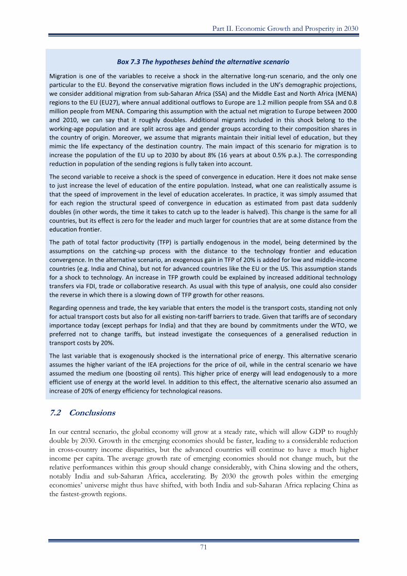
Part II. Economic Growth and Prosperity in 2030
71
Box 7.3 The hypotheses behind the alternative scenario
Migration is one of the variables to receive a shock in the alternative long-run scenario, and the only one
particular to the EU. Beyond the conservative migration flows included in the UN’s demographic projections,
we consider additional migration from sub-Saharan Africa (SSA) and the Middle East and North Africa (MENA)
regions to the EU (EU27), where annual additional outflows to Europe are 1.2 million people from SSA and 0.8
million people from MENA. Comparing this assumption with the actual net migration to Europe between 2000
and 2010, we can say that it roughly doubles. Additional migrants included in this shock belong to the
working-age population and are split across age and gender groups according to their composition shares in
the country of origin. Moreover, we assume that migrants maintain their initial level of education, but they
mimic the life expectancy of the destination country. The main impact of this scenario for migration is to
increase the population of the EU up to 2030 by about 8% (16 years at about 0.5% p.a.). The corresponding
reduction in population of the sending regions is fully taken into account.
The second variable to receive a shock is the speed of convergence in education. Here it does not make sense
to just increase the level of education of the entire population. Instead, what one can realistically assume is
that the speed of improvement in the level of education accelerates. In practice, it was simply assumed that
for each region the structural speed of convergence in education as estimated from past data suddenly
doubles (in other words, the time it takes to catch up to the leader is halved). This change is the same for all
countries, but its effect is zero for the leader and much larger for countries that are at some distance from the
education frontier.
The path of total factor productivity (TFP) is partially endogenous in the model, being determined by the
assumptions on the catching-up process with the distance to the technology frontier and education
convergence. In the alternative scenario, an exogenous gain in TFP of 20% is added for low and middle-income
countries (e.g. India and China), but not for advanced countries like the EU or the US. This assumption stands
for a shock to technology. An increase in TFP growth could be explained by increased additional technology
transfers via FDI, trade or collaborative research. As usual with this type of analysis, one could also consider
the reverse in which there is a slowing down of TFP growth for other reasons.
Regarding openness and trade, the key variable that enters the model is the transport costs, standing not only
for actual transport costs but also for all existing non-tariff barriers to trade. Given that tariffs are of secondary
importance today (except perhaps for India) and that they are bound by commitments under the WTO, we
preferred not to change tariffs, but instead investigate the consequences of a generalised reduction in
transport costs by 20%.
The last variable that is exogenously shocked is the international price of energy. This alternative scenario
assumes the higher variant of the IEA projections for the price of oil, while in the central scenario we have
assumed the medium one (boosting oil rents). This higher price of energy will lead endogenously to a more
efficient use of energy at the world level. In addition to this effect, the alternative scenario also assumed an
increase of 20% of energy efficiency for technological reasons.
7.2 Conclusions
In our central scenario, the global economy will grow at a steady rate, which will allow GDP to roughly
double by 2030. Growth in the emerging economies should be faster, leading to a considerable reduction
in cross-country income disparities, but the advanced countries will continue to have a much higher
income per capita. The average growth rate of emerging economies should not change much, but the
relative performances within this group should change considerably, with China slowing and the others,
notably India and sub-Saharan Africa, accelerating. By 2030 the growth poles within the emerging
economies’ universe might thus have shifted, with both India and sub-Saharan Africa replacing China as
the fastest-growth regions.

The Global Economy in 2030: Trends and Strategies for Europe
72
The three largest economies in the world will remain the same as today: the US, the EU and China.
However, the relative weights will shift within this ‘troika’, with China changing from the smallest to
becoming the largest (while the EU’s weight will remain close to that of the US).
A large part of the world should shift from low to middle-income levels, which should lead to an
explosion of the middle class in these countries. The expectations of this jump in the middle class, leading
to a consumption boom, are probably not likely to be fulfilled, but a world with a much larger middle
class and lower cross-country income differentials should experience fewer tensions, both economically
and politically.
Box 7.4 Heterogeneity within regions
We have reported only the averages for the major regions, like the EU, China and the US. But these large
economies obviously do not constitute homogenous units. Our study cannot deal with the details of the
differences within China, the US or Europe. The table below can give an impression of the degree of diversity
across major regional sub-units within these major economies.
We present two measures of the inter-regional variability within the three largest global economic units based
on the available data for GDP per capita. The most relevant one might be the standard deviation of income per
capita relative to the national average weighted by population. A second measure of regional heterogeneity is
simply the ratio of the region with the highest GDP per capita to the one with the lowest.
The table below suggests that the US is the least heterogeneous of these three large economies. Despite the
rather small average size of the sub-unit considered here (the average population per state is only about 6
million) the (weighted) standard deviation of relative income per capita is only about 15% and the richest state
has an income per capita that is ‘only’ twice as high of that of the poorest (excluding the special case of the
District of Columbia). By contrast, for the EU of 2010, the richest member state has an income per capita about
nine times higher than that of the poorest, even if one excludes an outlier like Luxembourg. This higher ratio is
significant, also because the average size of a member state is about three times that of a US state and a larger
unit is likely to provide for some averaging within its borders. The weighted standard deviation of relative
income per capita in the EU is at 36% (for 2010) – more than twice as high as the value for the US.
The diversity of income per capita across Chinese provinces seems to be (for the 2010 data) at a similar level to
the diversity across EU member states, although the average size of a Chinese province is over 40 million
inhabitants – about twice that of an average member state. The richest province has an income per capital
about six times higher than the poorest (which is less than the same ratio for the EU). But the weighted
standard deviation across provinces is, at 44%, somewhat higher than the corresponding value for 2010 for the
EU.
Heterogeneity within the major global economies
Country Weighted standard deviation in % of
average
High/Low Number of observations Average population (mn)
US 2010 15.0 2.2 50 states 6.2
China 2000 48.0 9.5 31 provinces 40.1
China 2010 43.9 5.8 31 provinces 43.0
India 2010 49.6 11.8 32 states 37.8
EU 2010 36.4 8.9 26 member states 19.3
EU 2030 27.5 4.8 23 member states 22.2
Note: Standard deviation is weighted by population. Luxembourg excluded for EU and Washington, D.C. excluded for the US.
Data on Slovenia, Cyprus and Malta are not available for the EU in 2030.
India seems to be the most heterogeneous of the continental-sized economies, given that it has the worst
indicator on both accounts.

Part II. Economic Growth and Prosperity in 2030
73
It is also interesting to note that in China both regional cohesion indicators have actually improved in the
decade up to 2010. Contrary to the widespread impression, the gap between the richest and the poorest
province has actually narrowed and the weighted standard deviation has fallen.
For the EU we have country-by-country projections of growth from the model. As expected, the model predicts
that the next decades should be characterised by convergence within the EU, reducing disparities in income
per capita. By 2030, the richest-to-poorest ratio should have halved to about 4.8 and the standard deviation
should be considerably lower.
8. The impact of growth on affluence and poverty
One element that emerges from the model simulations is that by 2030, differences in economic
performance should be much reduced. This applies both to levels of GDP per capita (however measured)
and growth rates. Convergence in (per capita) income levels is a simple result of the fact that advanced
economies will grow much more slowly than the poorer, emerging ones.
The most widely used measure of inequality is the Gini coefficient, which measures the shares that
different parts of the population have in overall income. If one limits one’s attention to the members of
the G20, which account for most of world’s income, one finds that the Gini coefficient in terms of GDP
per capita has already fallen from close to 0.6 to 0.5. Under the central scenario, this coefficient would by
2030 have fallen further to about 0.35, which is comparable to the level of inequality that one observes
within many countries. Income will thus be distributed much more equally across nations than it is today,
and the degree of cross-country inequality would no longer be much higher than the degree of inter-
personal inequality one observes today within many countries.76
The model also implies that growth in the more advanced EMEs will decelerate. This implies that by
2030 the differences in growth rates might also start to narrow, both within the emerging world and
between the group of emerging countries and the more advanced ones. This will particularly be the case
for China, where the growth rate is expected to fall to 6%, down from 8-10% recently, while other
countries like India and Indonesia are likely to experience an acceleration of growth.
Affluence will be more widely spread. This is not surprising given robust growth in the emerging
economies. One particular measure of the spread of affluence is the size of the ‘middle class’. This is of
particular interest both to political scientists and producers of consumer goods. The former are interested
in the size of the middle class because it is widely assumed that democracy is more likely to be stable in
countries with a large middle class. The latter are interested in the size of the middle class because of the
demand for consumer goods that is expected to follow.
The middle classes almost everywhere in the developing world are poised to expand substantially, in
terms of both absolute numbers and the percentage of the population that can claim middle-class status.
Even the more conservative models see a rise in the global total of those in the middle class from the
current one billion or so to over two billion people. Others see even more substantial rises with, for
example, the global middle class reaching three billion people by 2030. According to the definition
offered by Kharas & Gertz (2010) of the middle class – persons who spend between $10 and $100 a day
in PPP terms – the middle class will increase to 3.2 billion by 2020 and to 4.9 billion by 2030, almost one
half the world’s total population of 8.3 billion (Figure 8.1 shows the projected distribution across
76 The decrease in cross-country inequality may go hand-in-hand with a continued increase in inequality within each country. The US constitutes the best-known, but not the only case: data clearly indicate that income inequality has increased in most European countries compared to the 1970s and 1980s, a trend mirrored in a great majority of OECD countries over the past three decades, independent of their starting points. But the future evolution of income inequality within countries is extremely difficult to forecast. We have therefore not attempted to provide forecasts for this factor.

The Global Economy in 2030: Trends and Strategies for Europe
74
regions).77 Most of the studies reviewed agree that the most-rapid growth of the middle classes will occur
in Asia, with India somewhat ahead of China over the long term.
Figure 8.1 Middle class population by region, in 2012 and 2030 (millions)
Source: Kharas & Gertz (2010).
The very rapid increase in the middle class is a natural consequence of a threshold effect. If one takes a
country in which GDP per capita is just high enough so that 90% of the population has just enough
income to pay for basic food and shelter, one would find a very small middle class, probably less than 5%
of the population (the rest is the elite). If in such a country average income per capita doubles (without
any increase in inequality), a very large proportion of the population (possibly one-half) might attain
middle-class status because they would now have a substantial proportion of their income left (after basic
food and shelter). This implies that a doubling of income per capita can result in a middle class that is ten
times larger.
However, the economic impact of a growing middle class in EMEs on the advanced economies is likely
to be highly overrated in the current debate. Even if more than half of the world’s population becomes
middle class, their income will be far too low in most emerging economies to be a source of foreign
demand for expensive European or US goods. The economic impact of the ‘rise of the middle class’ will
remain confined to the domestic economy. Demand for consumer goods, including cars, of course rises
sharply with the growth of the middle class. In terms of consumption expenditure, by 2030 China and
India will have by far the biggest middle classes in the world, while the US middle class will be ranked
third in terms of consumption power, followed by Indonesia, which does not even rank among the top
ten today (NIC, 2012). Europe and North America’s share of global middle-class consumption is
expected to decrease from 64% in 2009 to 30% in 2030. By contrast, the share in consumption of the
Asia-Pacific middle class is estimated to increase from 23% to 59% over the same period. Some estimates
see middle-class consumption in North America and Europe rising by only 0.6% a year over the next
couple of decades.
One should keep in mind, however, that the middle class can expand only if productivity increases
enough to justify higher wages and salaries. While the consumption demand of the middle class in the
emerging Asian economies might grow very quickly, so will the productivity of the workers in these
countries. In many of them the middle class has actually tended to save a growing part of their higher
incomes. It is thus not certain that the growth of the middle class will automatically lead to a consumption
boom.
The acceleration of growth in emerging economies is not only creating a huge middle class – it is also
having a dramatic impact on poverty. In 1990, 43% of the population of developing countries lived in
77 Belonging to the middle class is usually associated with meeting “basic needs and affording a few extras” (Wheary, 2009). Relative approaches define the middle class as a middle segment within the income distribution scale of a given country. Absolute approaches, however, are better suited for international comparisons.

Part II. Economic Growth and Prosperity in 2030
75
extreme poverty (then defined as subsisting on $1 a day); that percentage has fallen to about 20% today.
The reduction in the absolute numbers is of course smaller because of population growth. The number of
persons categorised as ‘extreme’ poor has fallen from 1.9 billion in 1990 to 1.2 billion today.
As long as growth in the developing countries continues, poverty will also continue to fall, but it is
difficult to forecast by how much. Some estimates suggest that every 1% increase in GDP per head
reduces poverty by around 1.7%. This would be compatible with the experience of China, where the
poverty rate fell from 84% in 1980 to about 10% today. Other countries have lower growth rates and
could thus expect to benefit from a similar relationship between income growth and poverty reduction.
However, once income per capita goes beyond the point at which average income is just above the
poverty line, income distribution begins to matter.
Figure 8.2 Number of people in poverty (mn)
Source: Chandy et al. (2013, pp. 11-12).
A recent Brookings study (Chandy, Ledlie & Penciakova, 2013) provides an in-depth analysis of this
phenomenon by looking at the proportions of households that have an income close to the poverty line
(now defined as $1.25 in 2005 prices). They show that in many countries the most numerous group was,
in 1990, below the poverty line (and then a long tail of less numerous households with much higher
income). This has now changed with the most numerous group in some countries being those with an
income just above the poverty line. China constitutes the best example of this case, as shown in Figure
8.2. This shift has accounted for the rapid fall in poverty rates over the last two decades. There are also
still some countries, however (mainly in SSA) where the most numerous group is still below, but close to
the poverty line, with India being the most important case in point. This is where the strongest reduction
in poverty can be expected by 2030, as can be seen by the line depicting the 2030 forecast for India in the
figure below. Finally, there are those countries where even in 2030 the most numerous group will have an
income below the poverty line. This will be the case in most of SSA. By 2030 it thus likely that poverty
will be concentrated, with much of it in SSA and a large part of the remainder in parts of India.
Official development policy will have to be redesigned if the fall in levels of poverty proceeds as one can
expect. By 2030, most of the world’s poor (maybe about two-thirds) will live in ‘fragile’ states, i.e.
countries where there is no government that could effectively constitute a counterpart for foreign aid
agencies. There will of course also still be a substantial number of poor in countries whose average
income per capita is substantially above the poverty line. This might be the case in those states of India
where the basic education system is not functioning properly. But the entire country (in this case India)
would have enough resources to look after its own poor and it is unlikely that foreign aid agencies will
succeed in reforming basic education in those parts of the country where the federal government has not
been able to do so for decades.
9. The impact of growth on climate change
Climate change is a slow-moving process, driven by the accumulation of greenhouse gases (GHG) in the
atmosphere that – according to most models – will ultimately lead to major disruptions to long-term
weather patterns.

The Global Economy in 2030: Trends and Strategies for Europe
76
Global GHG emissions continue to increase at a fast rate. In May 2013, carbon-dioxide (CO2) levels in
the atmosphere exceeded 400 parts per million (ppm) for the first time in several hundred millennia and
are up from about 280 ppm in pre-industrial times (IEA, 2013a).
The average global air temperature has risen steadily – about 0.8°C since 1880, according to the latest
NASA analysis.78 In 2012 the average global temperature was about 0.6°C warmer than the mid-20th
century baseline. The 2007 report by the International Panel on Climate Change (IPCC, 2007a) suggested
that global mean temperatures could rise by as much as 1.8-4.0°C over the course of this century if global
action to limit GHG emissions fails. The IEA (2013a) estimates that the world is currently on a trajectory
towards an average temperature increase of between 3.6°C and 5.3°C by the end of this century.
Human-induced climate change is driven mostly by GHG emissions. These are largely due to the use of
fossil fuels, although deforestation, land-use change and agriculture also provide significant but smaller
contributions. The major drivers therefore are global population growth, increases in demand for food,
water and energy and agricultural practices.
The range between 1.8°C and 4°C (IPCC, 2007a) or 3.6°C and 5.3°C (IEA, 2013a) suggests that there is
great uncertainty about the projections. Major uncertainties also remain about the impact on human
society, including long-term health effects, regional conflicts, migration and political instability.
Irrespective of these uncertainties, there is little doubt that climate change is a major challenge for the EU
and the world at large. Nevertheless, whatever happens before 2030 in terms of climate and emissions has
largely already been determined, so any policy change today or in the near future will mainly have an
impact in the post-2030 period. The capital stock until 2030 both in the EU and globally is largely
deployed, meaning that major changes in the emissions trajectories are most likely to take effect only after
2030. This seems to be also the conclusion of the IEA (2013a), which sees that reductions of GHG
emissions would mainly come from specific add-on policies, i.e. regulation rather than long-term
structural change of the capital stock79 in a 2035 perspective.
It is also unlikely that major climate changes will have taken place by 2030. The latest IPCC report (IPCC
2013) writes that that the mean global mean surface air temperature for the period until 2035 will ‘very
unlikely’ be more than 1.5°C80 above the 1850-1900 mean. This prediction is below the threshold where
major climate change impacts are expected and is in line with previous studies on impacts and adaption,
which almost exclusively focus on and therefore identify impacts after the 2030 period.81 Economically,
most analyses conclude that climate change impacts at these warming levels are manageable. This might
change with increasing warming, but such changes will in all likelihood only take effect beyond 2030.
9.1 The predictions of the model on climate change
The model we employ can also be used to calculate a time path for global emissions, but this yields
different results from most other studies. The reason is a fundamental difference in approach – in essence
a clash between ‘engineers’, ‘scientists’ and ‘economists’.
The approach used by the MaGE model is a purely economic one. It starts from the basic proposition
that energy and CO2 emissions will continue to grow proportionally to GDP unless relative prices change
considerably. The latter is not the case because oil prices are projected to increase only moderately and
the likelihood that there will be substantial carbon pricing outside the EU is at present rather low. There
78 NASA Goddard Institute for Space Studies (see http://data.giss.nasa.gov/gistemp/). 79 Half of the identified reduction potential would be achieved by adopting specific energy-efficiency measures. Other measures limit the construction and use of the least-efficient coal-red power plants by a further 20%, while minimising methane emissions from upstream oil and gas production, e.g. stopping flaring and phasing-out of subsidies to fossil-fuel consumption would account for the rest (IEA 2013a).
80 The projected change in global mean surface air temperature will likely be in the range 0.3–0.7°C (IPCC, 2013).
81 For a literature overview, see Egenofer et al. (2010).
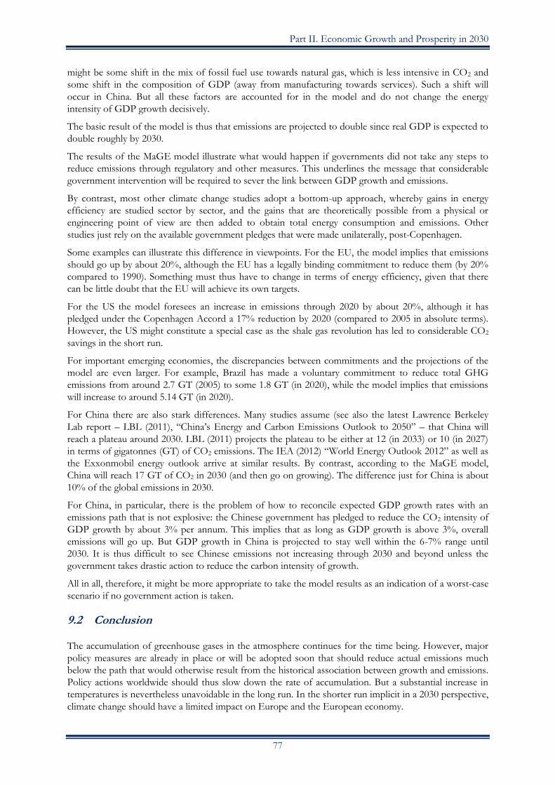
Part II. Economic Growth and Prosperity in 2030
77
might be some shift in the mix of fossil fuel use towards natural gas, which is less intensive in CO2 and
some shift in the composition of GDP (away from manufacturing towards services). Such a shift will
occur in China. But all these factors are accounted for in the model and do not change the energy
intensity of GDP growth decisively.
The basic result of the model is thus that emissions are projected to double since real GDP is expected to
double roughly by 2030.
The results of the MaGE model illustrate what would happen if governments did not take any steps to
reduce emissions through regulatory and other measures. This underlines the message that considerable
government intervention will be required to sever the link between GDP growth and emissions.
By contrast, most other climate change studies adopt a bottom-up approach, whereby gains in energy
efficiency are studied sector by sector, and the gains that are theoretically possible from a physical or
engineering point of view are then added to obtain total energy consumption and emissions. Other
studies just rely on the available government pledges that were made unilaterally, post-Copenhagen.
Some examples can illustrate this difference in viewpoints. For the EU, the model implies that emissions
should go up by about 20%, although the EU has a legally binding commitment to reduce them (by 20%
compared to 1990). Something must thus have to change in terms of energy efficiency, given that there
can be little doubt that the EU will achieve its own targets.
For the US the model foresees an increase in emissions through 2020 by about 20%, although it has
pledged under the Copenhagen Accord a 17% reduction by 2020 (compared to 2005 in absolute terms).
However, the US might constitute a special case as the shale gas revolution has led to considerable CO2
savings in the short run.
For important emerging economies, the discrepancies between commitments and the projections of the
model are even larger. For example, Brazil has made a voluntary commitment to reduce total GHG
emissions from around 2.7 GT (2005) to some 1.8 GT (in 2020), while the model implies that emissions
will increase to around 5.14 GT (in 2020).
For China there are also stark differences. Many studies assume (see also the latest Lawrence Berkeley
Lab report – LBL (2011), “China’s Energy and Carbon Emissions Outlook to 2050” – that China will
reach a plateau around 2030. LBL (2011) projects the plateau to be either at 12 (in 2033) or 10 (in 2027)
in terms of gigatonnes (GT) of CO2 emissions. The IEA (2012) “World Energy Outlook 2012” as well as
the Exxonmobil energy outlook arrive at similar results. By contrast, according to the MaGE model,
China will reach 17 GT of CO2 in 2030 (and then go on growing). The difference just for China is about
10% of the global emissions in 2030.
For China, in particular, there is the problem of how to reconcile expected GDP growth rates with an
emissions path that is not explosive: the Chinese government has pledged to reduce the CO2 intensity of
GDP growth by about 3% per annum. This implies that as long as GDP growth is above 3%, overall
emissions will go up. But GDP growth in China is projected to stay well within the 6-7% range until
2030. It is thus difficult to see Chinese emissions not increasing through 2030 and beyond unless the
government takes drastic action to reduce the carbon intensity of growth.
All in all, therefore, it might be more appropriate to take the model results as an indication of a worst-case
scenario if no government action is taken.
9.2 Conclusion
The accumulation of greenhouse gases in the atmosphere continues for the time being. However, major
policy measures are already in place or will be adopted soon that should reduce actual emissions much
below the path that would otherwise result from the historical association between growth and emissions.
Policy actions worldwide should thus slow down the rate of accumulation. But a substantial increase in
temperatures is nevertheless unavoidable in the long run. In the shorter run implicit in a 2030 perspective,
climate change should have a limited impact on Europe and the European economy.

The Global Economy in 2030: Trends and Strategies for Europe
78
The biggest burden for Europe might result from the very high cost of avoiding emissions in today’s
main sources of renewable energy, namely wind and photovoltaic solar. However, as other key
technologies (CCS, storage, offshore wind) remain very much uncertain, it is difficult to determine the
economic cost of a decarbonisation of growth and the extent to which it will differ across the major
global economies.
Cost is one element. An even more important element in the policy debate that is likely to continue up to
2030 will of course be the evolution of the climate itself. Policy action is much more likely to be taken
everywhere if climate patterns change as predicted or if extreme events bear witness to the warnings that
climate change carries large potential risks.

79
Part III. The EU’s Transition towards 2030
The horizon up to 2030 is sufficiently far away to warrant a long-term view in which markets are in
equilibrium and no major disequilibria persist. However, 2030 is also sufficiently close to make the
transition to the long-term equilibrium a relevant issue. This is relevant for Europe and for the eurozone.
By 2030 the euro crisis should only be a distant memory, but much of the time until 2030 might be
marked by the adjustment process in the peripheral countries of the euro area.
We used the NEMESIS model (see Annex D) to provide insights into how the European economy can
transit from the present situation of high unemployment and exploding government debt to (hopefully) a
more stable combination of ‘normal’ levels of employment and stable government finances in 2030.
A first lesson from taking this medium-term view is that the demographic decline of Europe acquires a
slightly different angle. The working-age population of Europe will soon start to decline, as documented
earlier in this report, but given the very high unemployment rates in Europe today it is likely that overall
employment will increase between now and 2030. For some time the main factor holding back growth in
Europe might thus be demand rather than supply, given that significant underutilised resources exist in
terms of high unemployment (and, in some countries, low labour-force participation) rates.
It is also apparent that the economic path must be very different for the countries in the euro-area
periphery struggling with an adjustment to a sudden stop in the capital flows, which until recently had
financed domestic consumption and investment. In these countries the non-tradable sector must shrink
and the tradable sector must expand. But shifting factors of production – especially labour – between the
two requires time. Countries like Spain are thus likely to have high unemployment for quite some time.
Until now the adjustment process within the euro area has been asymmetric, with contraction of demand
in the periphery, but no corresponding expansion of demand in the core countries, notably Germany.
For these reasons we present the results for three types of countries:
1) The northern countries, represented by Germany, which starts with a positive external balance
and relatively low unemployment rates.
2) The peripheral southern group of countries, where the external balance was in deficit and
unemployment is now very high, as represented by Spain.
3) Finally, the newer member states from the east (illustrated here by Poland) for which productivity
growth remains fast, due to a structural and a catching-up effect.
As we will see, the path for all groups is mainly driven by world demand, demography and the
relationship between productivity and real wages. Productivity is thus at the core of the competitiveness,
growth and employment triangle.
The spirit of this baseline is not that of a ‘forecast’ but a coherent scenario based on a model of how the
European economy works. Details of the NEMESIS simulations are presented in Annex D. They reveal
some interesting predictions, which might appear unconventional at first sight. For example, a
considerable fall in the share of employment in industry in Germany might be expected. The public debt
and fiscal deficits of southern countries are likely to remain higher and longer over the period than

The Global Economy in 2030: Trends and Strategies for Europe
80
officially planned (and permitted under the Fiscal Compact).82 More in general, these results reveal the
difficulties of emerging from crisis in a context of low growth and weak productivity in the EU.
The next sections are based on the main results of the model.
10. The outcome of the NEMESIS model: Introduction
We present the results of an exercise based on a simulation using the NEMESIS model for the 27
member states of the European Union. To ensure consistency between findings at global and European
level, the exogenous variables of the model are set in accordance with the findings of the MaGE model.
The main added value of this exercise is its coherency within a detailed accounting framework which links
together every European country and every economic sector with econometric behavioural equations.
The time path shown below runs from the global crisis that started in 2008 with the beginning of the
labour force decline and sources of major shocks, through to the sovereign debt crisis, with its
consequences for interest rates and economic growth, and labour market disequilibrium and its
implications for wages. One major concern, when looking to the past, is the evolution of labour
productivity: the countries hardest hit by the crisis were those with the lowest productivity gains prior to
2007. Productivity will therefore be at the core of our analysis, all the more so because productivity gains
after the crisis will not rebound to pre-crisis levels. A second concern is ageing and the decline of the
labour force in the second phase of the period. How can the transition towards this demographic stress
be managed when the effects of the crisis fade, leaving weak unemployment rates for certain countries?
Europe as a whole is made up of very heterogeneous countries in terms of structure, demography,
productivity, economic growth and other criteria. The diagnosis on Europe must therefore be completed
by a more detailed approach to the different countries, which will allow us to classify them into one of
three categories: the northern European countries with high productivity, the southern European
countries hardest hit by crisis, and the eastern European countries. Regarding finance, the level of
sovereign debt is a crucial issue in almost all countries, except in some eastern ones, but with relevant
differences. This implies a high level of debt burden, despite the objective of decreasing public deficits
that weighs on public expenditure. Deleveraging is difficult for some countries that are in a debt trap
(high interest rates, less public expenditure, less growth, less taxation revenues, etc.). Furthermore, the
main cause of the disease in the scenario is linked to productivity gains: after the crisis, the rebound (to
1.2%) will be insufficient to reach the level of productivity gains before the crisis (1.5-1.6%).
We end our exercise with what we might call a ‘normative’ experiment. How would the scenario change if
we could revert to the 1.6% level, that is to say, if the productivity gains were higher by 0.4% every year?
It is a normative exercise since we do not describe the measures to be taken in order to reach this level of
productivity growth, and the productivity shock introduced in the model is exogenous. Nevertheless, we
did allocate these extra productivity gains proportionally to the innovation capacities of the different
countries.
11. Europe as whole
We concentrate here on the results for the EU. The average growth rate for the EU is expected to
rebound after the present recession, but only to about 1.5%. Medium-term growth might then drop to
about 1.2%. More important than this headline figure, however, are the components shown in the figure
below. The key driver of growth is initially the foreign (trade) balance, whose contribution remains
positive until about 2020, whereas consumption is predicted to remain weak in the near term, but should
82
Fiscal Compact (formally known as the Treaty on Stability, Coordination and Governance in the Economic and
Monetary Union; also referred to as TSCG), is an intergovernmental treaty introduced as a new, stricter version of the previous Stability and Growth Pact of 2012.

Part III. The EU’s Transition towards 2030
81
become stronger over time. In essence, the EU will experience a ‘rebalancing’ similar to that occurring in
China today. The problem for Europe is that the levers to foster consumption growth are much weaker
than in China, where, at least a priori, there should be a huge potential of unmet demand for many
consumer goods that are already universal in Europe.
Under this scenario, unemployment in the EU would fall slowly but steadily and roughly by half by 2030.
This would then allow employment to be higher, by about 5 million units, although the population in
working age will have fallen.
Figure 11.1 Contribution of main components to the growth of GDP for EU27 (2010-30)
All in all, these results suggest that the EU economy should be able to reach a longer-term equilibrium,
which forms the basis of the central scenario used here. But the transition might be rather long.
We first present the results for Europe as a whole. We will emphasise the macro-dynamics, and then give
some insights on the sectoral aspects. What we can see, at a first glance, is that the macro-dynamics of the
period are mainly the result of the interaction between real wage growth and productivity growth, which
explains the evolution of GDP components and growth. Three consecutive phases follow: the
competitiveness, the rebound in productivity and the slowing down of competitiveness.
11.1 The first phase (2011-14): External balance the main driver for GDP
During the first phase, GDP falls and then labour productivity slows down, but after three years of crisis,
unemployment is high and wage growth is very low under the productivity gains. Europe then increases
its price competitiveness and benefits fully from the resumption in global demand in 2011. We can see in
Figure 11.2 that, in spite of the slowing down of labour productivity gains, wage growth stays below
productivity growth. In fact, when we look at GDP growth for the period, we can see that it is the
external balance that prevents GDP growth from collapsing and that up to 2014-15, external surpluses are
the main drivers for GDP growth (Figure 11.2). The share of consumption in GDP decreases and is
replaced by external surpluses. This is a consequence of wage decreases and of rises in unemployment
that reach a peak of 10.6% in 2013, while the inflation rate is at its lowest level.
-0.5%
0.0%
0.5%
1.0%
1.5%
2.0%
20
10
20
12
20
14
20
16
20
18
20
20
20
22
20
24
20
26
20
28
20
30
GDP
Private consumption
Investment
Public consumption
Trade Balance

The Global Economy in 2030: Trends and Strategies for Europe
82
Figure 11.2 Labour productivity and real wage growth rates for the EU27
Table 11.1 GDP and components: Level in 2010 (€ bn in 2005 dollars)
and average annual growth rates
2010* 2010-15 2015-20 2020-25 2025-30
GDP 11,504.3 0.85 1.55 1.46 1.39
Private consumption 6,582.1 0.25 1.15 1.47 1.72
Public consumption 2,517.1 0.06 1.03 1.22 1.21
Gross fixed capital formation 2,218.6 0.99 2.82 2.12 1.88
Exports 4,149.0 4.01 3.61 2.61 1.92
Imports 3,885.7 2.93 3.69 2.99 2.51
GDP per capita (K€/cap)** 23,045 23,747 25,379 27,137 28,908
* Level in billions of 2005 euros.
** At the end of the period.
During the first period, government deficits are reduced. However, the debt burden is such that sovereign
debt increases by a significant proportion, as it is a period of low nominal growth (inflation and growth
are very weak). These dynamics of productivity are all explained here by the ‘productivity cycle’; the
second phase starts with the end of this cycle.
Table 11.2 Contribution to GDP growth (annual average point of GDP growth rate)
Contribution to GDP growth* 2010-15 2015-20 2020-25 2025-30
GDP growth 0.85 1.55 1.46 1.39
Private consumption 0.14 0.63 0.80 0.94
Public consumption 0.01 0.21 0.25 0.25
Gross fixed capital formation 0.19 0.56 0.44 0.41
Trade balance 0.51 0.14 -0.04 -0.20
* In annual average point of GDP growth rate.
-0.5%
0.0%
0.5%
1.0%
1.5%
2.0%
20
10
20
11
20
12
20
13
20
14
20
15
20
16
20
17
20
18
20
19
20
20
20
21
20
22
20
23
20
24
20
25
20
26
20
27
20
28
20
29
20
30
labour productivity
real wage

Part III. The EU’s Transition towards 2030
83
11.2 The second phase (2014-18): The rebound in productivity
The second period starts with rebounds in productivity and in wages. The productivity rebound is
insufficient to reach the labour productivity growth rate that prevailed before 2007 (1.3% versus 1.7%),
but unemployment is such that wage growth is lower than productivity gains.
This lower productivity growth may be due to two phenomena that result from the crisis and the low
GDP growth since 2008: a substitution effect due to weak wages, and a slowing down of R&D volume
(although R&D effort as a proportion of GDP is not decreasing) due to GDP stagnation. The low wage
is due to the augmented Phillips curve of the NEMESIS model. The mechanisms linking labour
productivity to factor substitutions, R&D and human capital (skills) are of course reductive, as with all
modelling exercises. Moreover, we assumed that the crisis did not affect the structure of human capital.
Nevertheless, we believe that R&D variations are a major determinant of productivity gains in the long
term. Throughout the second phase, the growth rate of labour productivity being above the wage curve
allows for the accumulation of price competitiveness gains. With the world demand hypothesis, the
external balance will therefore increase, but at a slower pace than in the preceding phase.
GDP growth is then driven simultaneously by internal demand resulting from a rebound in wages and an
investment catching-up process, and by the external balance. GDP growth reaches its highest level
(around +1.62% in 2016) in the first part of this period, despite a slight increase in productivity growth,
and when real wages increase. One possible explanation for this is that unemployment falls continuously
over the period. For these reasons, the contribution of external balances to GDP growth decreases and
then growth falls at the end of the period. Nevertheless, the share of consumption’s contribution to GDP
decreases in favour of external balances throughout the period in question. The inflation rate also
rebounds, the public deficit decreases and the sovereign debt-to-GDP ratio starts to decrease very slowly.
11.3 Third phase (2019-30): Losses in competitiveness
The third phase starts when the real wage growth overtakes productivity gains (in 2019). Europe is then
losing price competitiveness, despite slow productivity gains. Falling unemployment increases real wages.
We can make two main remarks here. The first is on the wage curve used in the model: although the
labour market is far from representing a positive demand excess, wages increase. There has been much
debate on the credibility of this description of the labour market, around the concepts of structural
unemployment or of mismatching between supply and demand. Nevertheless, we believe that this
mechanism can provide a good description of the consequences of a stagnant active population in an
economic area.
The dynamic in the third phase is very different from that of the two first. Although the trade balance still
represents an important part of GDP, its contribution to GDP growth (Table 11.2) soon becomes
negative, and GDP growth in volume then declines until it reaches 1.4% in 2030. This decline is
accompanied by slight inflationary pressures, and consequently the GDP growth in value is increasing
faster. For this reason, and also because the deficit reduction policy bears fruit, the debt-to-GDP ratio is
declining faster.
11.4 The labour market
The significant disequilibrium present at the beginning is progressively reduced and the unemployment
rate reaches 6% at the end of the period (2030). We can see that the fall in unemployment at the end
comes from a reduction in the labour force; growth cannot create new jobs in 2030.
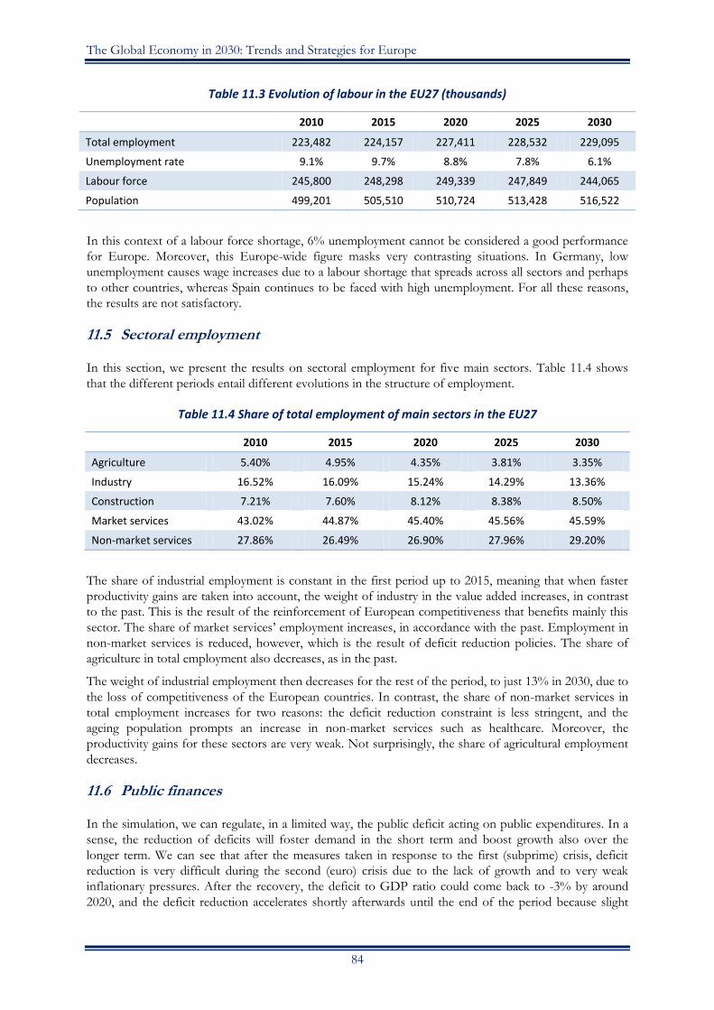
The Global Economy in 2030: Trends and Strategies for Europe
84
Table 11.3 Evolution of labour in the EU27 (thousands)
2010 2015 2020 2025 2030
Total employment 223,482 224,157 227,411 228,532 229,095
Unemployment rate 9.1% 9.7% 8.8% 7.8% 6.1%
Labour force 245,800 248,298 249,339 247,849 244,065
Population 499,201 505,510 510,724 513,428 516,522
In this context of a labour force shortage, 6% unemployment cannot be considered a good performance
for Europe. Moreover, this Europe-wide figure masks very contrasting situations. In Germany, low
unemployment causes wage increases due to a labour shortage that spreads across all sectors and perhaps
to other countries, whereas Spain continues to be faced with high unemployment. For all these reasons,
the results are not satisfactory.
11.5 Sectoral employment
In this section, we present the results on sectoral employment for five main sectors. Table 11.4 shows
that the different periods entail different evolutions in the structure of employment.
Table 11.4 Share of total employment of main sectors in the EU27
2010 2015 2020 2025 2030
Agriculture 5.40% 4.95% 4.35% 3.81% 3.35%
Industry 16.52% 16.09% 15.24% 14.29% 13.36%
Construction 7.21% 7.60% 8.12% 8.38% 8.50%
Market services 43.02% 44.87% 45.40% 45.56% 45.59%
Non-market services 27.86% 26.49% 26.90% 27.96% 29.20%
The share of industrial employment is constant in the first period up to 2015, meaning that when faster
productivity gains are taken into account, the weight of industry in the value added increases, in contrast
to the past. This is the result of the reinforcement of European competitiveness that benefits mainly this
sector. The share of market services’ employment increases, in accordance with the past. Employment in
non-market services is reduced, however, which is the result of deficit reduction policies. The share of
agriculture in total employment also decreases, as in the past.
The weight of industrial employment then decreases for the rest of the period, to just 13% in 2030, due to
the loss of competitiveness of the European countries. In contrast, the share of non-market services in
total employment increases for two reasons: the deficit reduction constraint is less stringent, and the
ageing population prompts an increase in non-market services such as healthcare. Moreover, the
productivity gains for these sectors are very weak. Not surprisingly, the share of agricultural employment
decreases.
11.6 Public finances
In the simulation, we can regulate, in a limited way, the public deficit acting on public expenditures. In a
sense, the reduction of deficits will foster demand in the short term and boost growth also over the
longer term. We can see that after the measures taken in response to the first (subprime) crisis, deficit
reduction is very difficult during the second (euro) crisis due to the lack of growth and to very weak
inflationary pressures. After the recovery, the deficit to GDP ratio could come back to -3% by around
2020, and the deficit reduction accelerates shortly afterwards until the end of the period because slight

Part III. The EU’s Transition towards 2030
85
inflationary pressures compensate for the slowdown in growth. Indeed, this reveals the difficulty of
decreasing the debt to GDP ratio in the first part of the period. This global diagnosis also covers very
heterogeneous evolutions; as we said in the Introduction, some countries could fall into a ‘debt trap’.
Figure 11.3 Public finance in the EU27
12. A more detailed approach
If Europe as a whole consists of very heterogeneous countries, we can look for criteria to categorise these
countries and to present the results in a synthetic way. The first and simplest idea is to use GDP per
capita at the beginning (2010). We will see that this is a relevant criterion as it can explain the future
dynamic of countries (perhaps because it is guided by a certain convergence, as we will see).
12.1 Characteristics of the three types of country
Figure 12.1 shows that in 2010 there was a group of northern European countries with the highest GDP
per capita levels, followed by the southern European countries, and finally the eastern European
countries.
Northern Europe (e.g. Germany) was in a better position in terms of competitiveness before the crisis. Its
public balance was less degraded and its trade balance was positive. Northern European economies had
experienced a moderate increase in wages in the years before the crisis, so labour productivity increased at
a higher rate than wages, leading to the gain in competitiveness. Although they experienced a severe
recession in 2009, the situation of the Nordic countries is the least dramatic among European countries,
as they do not suffer from a situation of twin deficits (i.e. public accounts and trade balance both in
deficit).
In the decade preceding the crisis, southern Europe (e.g. Spain) had experienced a huge increase in wages,
which was not compensated for by a similar increase in labour productivity. These economies have thus
lost competiveness and seen deterioration in their external balance. The dynamism of consumption in
these countries also weighed negatively on their external accounts. Before the crisis, growth relied mainly
on strong consumption and investment in the housing sector financed by debt. Their public accounts
were vulnerable and the magnitude of the crisis in these countries was high because of the large existing
debt that weakened these fragile public accounts. The debt burden in these countries has greatly
increased, as also has unemployment. These countries were the most heavily affected by the crisis,
provoking fear that the euro area would collapse.
74%
76%
78%
80%
82%
84%
86%
88%
90%
92%
20
10
20
12
20
14
20
16
20
18
20
20
20
22
20
24
20
26
20
28
20
30
General government gross debt (% of GDP)
-7%
-6%
-5%
-4%
-3%
-2%
-1%
0%
20
10
20
12
20
14
20
16
20
18
20
20
20
22
20
24
20
26
20
28
20
30
General government balance (% of GDP)

The Global Economy in 2030: Trends and Strategies for Europe
86
Figure 12.1 GDP per capita (2010) and average annual growth rate of GDP per capita (2010-30)
Eastern European countries (e.g. Poland) are in economic catch-up phase with the rest of Europe. In the
years prior to the crisis, they were a desirable location for industrial activity due to lower wages than in
western Europe. These countries had initially low levels of public debt. Even if their wages rose sharply,
they remained highly competitive due to the very low initial levels of labour costs. The economic
catching-up of these countries takes the form of a sustained labour productivity growth rate, and their
handicap is a declining labour force due to an ageing population.
12.2 The convergence
Figure 12.2 shows the initial levels of GDP per capita (in 2010) for the EU27 countries and their growth
rate over the period 2010-30. We observe that over the period, there is a clear convergence phenomenon
at work regarding the countries of northern Europe (illustrated in blue in our figure) and the countries of
eastern Europe (illustrated in green). Eastern European countries originally had lower levels of GDP per
head, but higher rates of GDP per capita growth. In contrast, the countries of southern Europe
(illustrated in orange) are in a situation of divergence with the rest of Europe. Starting off from a situation
of lower GDP per capita than the EU27 average in 2010, they also experience GDP per head growth
rates that are lower than the EU27 average.
It should nevertheless be noted that the beginning of the period is marked by the sovereign debt crisis in
the southern European countries, so it may be useful to distinguish two sub-periods in our scenario: the
‘end-of-crisis’ period with deleveraging until 2020 and a more regular period from 2020-30 during which
the usual forms of behaviour that characterised European economies before the crisis are at work (higher
growth and higher wage growth in the south, a trade deficit re-appearing in the south, and so on). That
said, we believe that the impact of the crisis is felt throughout the entire period of the scenario.
Figures 12.2 and 12.3 show the relationship between the level of initial GDP per capita and the growth
rate over the period for the two sub-periods of 2010-20 and 2020-30. We see that after a decade of
adjustment, deleveraging and deteriorating growth, the southern countries experience more significant
growth rates during the second period (2020-30), providing a relatively complete convergence
phenomenon for the EU27. To be more precise, the economic growth literature distinguishes two types
of convergence: ‘sigma-convergence’ is a reduction in the dispersion of GDP per capita or income levels
across economies, while ‘beta-convergence’ occurs when the economies with an initial low level of
income or GDP per capita grow faster. We can test for sigma-convergence by calculating the relative
0.0%
0.5%
1.0%
1.5%
2.0%
2.5%
3.0%
3.5%
4.0%
4.5%
0 5,000 10,000 15,000 20,000 25,000 30,000 35,000 40,000 ave
rage
an
nu
al g
row
th r
ate
of
GD
P p
er
cap
ita
fr
om
20
10
to
20
30
GDP per capita in 2010 (in euro per capita)
Lithuania
Latvia
Estonia
Bulgaria Slovakia
Romania Malta
Poland Czech Rep.
Hungary
Sweden Austria
Spain Greece United Kingdom
Denmark Germany
Belgium Finland
France
Cyprus Portugal
Italy
Slovenia
Ireland
Netherlands EU27

Part III. The EU’s Transition towards 2030
87
standard deviation of all GDP per capita in 2010, 2020 and 2030 (the ratio of the standard deviation to
the average of a data set). We find that there is indeed reduced dispersal of GDP per capita over the
entire period. In contrast, beta-convergence is only observed during the second sub-period (2020-30), as
during the first period necessary adjustments in the public accounts of the southern European countries
affect negatively their growth.
Figure 12.2 GDP per capita in 2010 and average annual growth rate of GDP per capita (2010-20)
Figure 12.3 GDP per capita in 2020 and average annual growth rate of GDP per capita (2020-30)
-1.5%
0.0%
1.5%
3.0%
4.5%
6.0%
0 5,000 10,000 15,000 20,000 25,000 30,000 35,000 40,000 ave
rage
an
nu
al g
row
th r
ate
of
GD
P p
er
cap
ita
fro
m 2
01
0 t
o 2
02
0
GDP per capita in 2010 (in euro per capita)
Lithuania
Latvia Estonia
Bulgaria
Slovakia Romania
Malta Poland
Czech Rep.
Hungary
Sweden Austria
Spain
Greece
UK
Denmark Germany
Belgium Finland
France
Cyprus
Portugal Italy
Slovenia
Ireland
Netherlands EU27
0.0%
0.5%
1.0%
1.5%
2.0%
2.5%
3.0%
3.5%
0 5,000 10,000 15,000 20,000 25,000 30,000 35,000 40,000 45,000 ave
rage
an
nu
al g
row
th r
ate
of
GD
P p
er
cap
ita
fr
om
20
20
to
20
30
GDP per capita in 2020 (in euro per capita)
Lithuania
Latvia Estonia
Bulgaria
Slovakia Romania
Malta
Poland Czech Rep.
Hungary
Sweden Austria
Spain
Greece
United Kingdom
Denmark
Germany
Belgium
Finland
France
Cyprus Portugal
Italy
Slovenia
Ireland
Netherlands EU27

The Global Economy in 2030: Trends and Strategies for Europe
88
12.3 Slow and incomplete adjustments for unemployment and deleveraging
Figure 12.4 summarises the dynamic adjustment at work in our scenario. The x-axis shows the growth
rate of real wages and the y-axis the growth rate of labour productivity. The 45° dotted line shows where
the growth rates of labour productivity and real wages are equal. Countries above this line experience
higher labour productivity growth than real wage growth, and thus enjoy increased competitiveness. This
is the case for the countries of southern Europe such as Spain. Countries below this line experience a loss
of competitiveness, as real wage growth is higher than that of labour productivity.
Figure 12.4 Average annual growth rate of labour productivity and real wages (2010-30)
This is the case for the countries of northern Europe such as Germany. Eastern European countries are
experiencing strong growth in labour productivity (catching-up), which offsets the dynamic growth in real
wages over the period.
One of the most striking elements of our scenario is that the unemployment rate and public debt (relative
to GDP) will not be able to reach the pre-crisis levels, not even by the end of the period.
Starting from an initial situation in which some of the eastern European countries have high levels of
unemployment and some of the countries of southern Europe have high levels of public debt (the
countries of northern Europe being in an intermediate situation), we find that the eastern European
countries are able to reduce their levels of unemployment, while the northern European countries reduce
both their level of unemployment (sometimes helped by the reduction of their labour force) and the
weight of their debt (see Figure 12.5). Southern European countries, however, reduce their
unemployment by very little over the period and the weight of their debt stabilises at best, but does not
fall.
Having roughly characterised the main features of the three groups of countries, Annex D presents a
deeper case analysis of each of the three groups: Germany for the northern European countries, Spain for
the southern European countries and Poland for the eastern European countries. In each presentation,
we explain the components of growth through a gap between productivity and real wages, then examine
the adjustments on the labour market and finally address the public finance situation.
0.0%
0.5%
1.0%
1.5%
2.0%
2.5%
3.0%
3.5%
4.0%
-0.5% 0.0% 0.5% 1.0% 1.5% 2.0% 2.5% 3.0% 3.5% 4.0%
Ave
rage
an
nu
al g
row
th r
ate
of
lab
ou
r p
rod
uct
ivit
y fr
om
20
10
to
20
30
Average annual growth rate of real wage from 2010 to 2030
Lithuania Latvia
Estonia
Bulgaria
Slovakia Romania
Malta Poland
Czech Rep.
Hungary
Sweden Austria
Spain Greece
United Kingdom
Denmark
Germany
Belgium
Finland
France
Cyprus
Portugal
Italy
Slovenia
Ireland Netherlands EU27
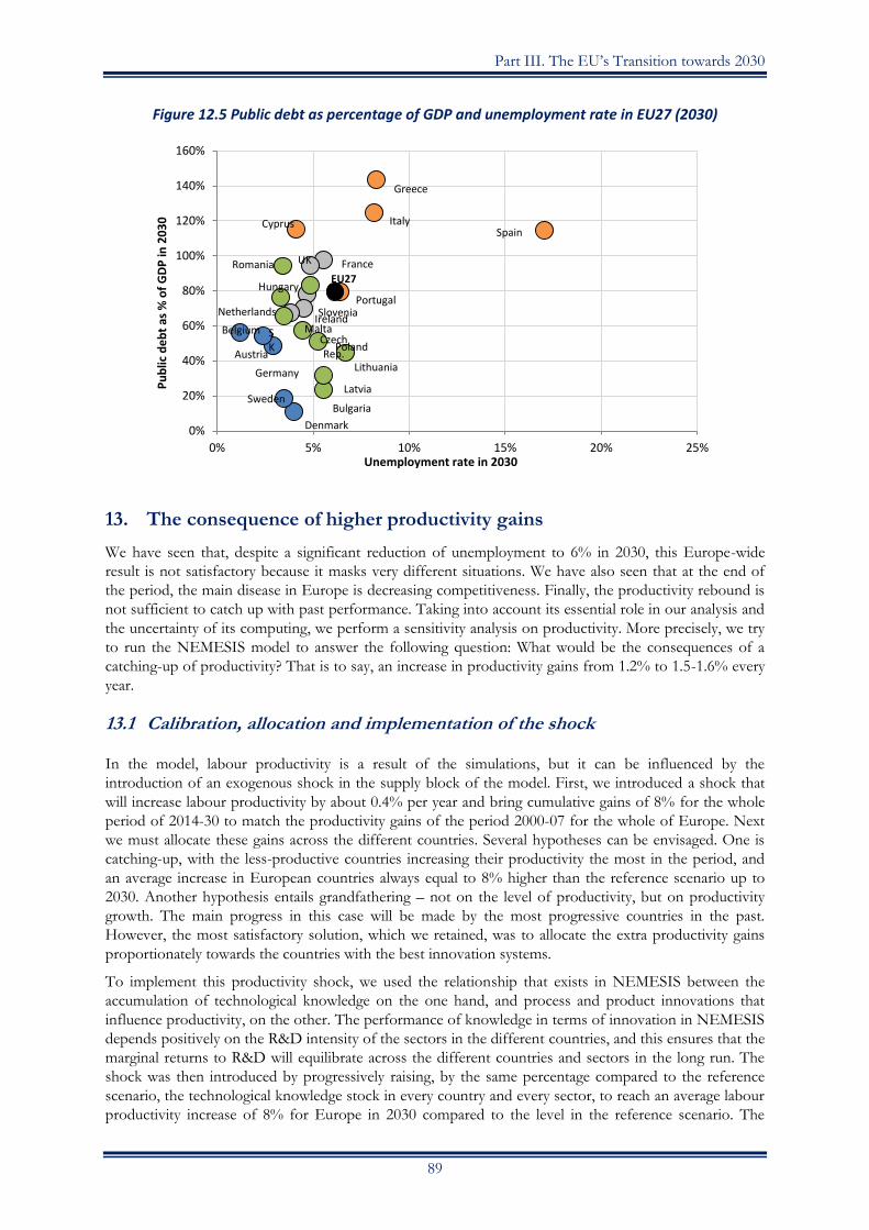
Part III. The EU’s Transition towards 2030
89
Figure 12.5 Public debt as percentage of GDP and unemployment rate in EU27 (2030)
13. The consequence of higher productivity gains
We have seen that, despite a significant reduction of unemployment to 6% in 2030, this Europe-wide
result is not satisfactory because it masks very different situations. We have also seen that at the end of
the period, the main disease in Europe is decreasing competitiveness. Finally, the productivity rebound is
not sufficient to catch up with past performance. Taking into account its essential role in our analysis and
the uncertainty of its computing, we perform a sensitivity analysis on productivity. More precisely, we try
to run the NEMESIS model to answer the following question: What would be the consequences of a
catching-up of productivity? That is to say, an increase in productivity gains from 1.2% to 1.5-1.6% every
year.
13.1 Calibration, allocation and implementation of the shock
In the model, labour productivity is a result of the simulations, but it can be influenced by the
introduction of an exogenous shock in the supply block of the model. First, we introduced a shock that
will increase labour productivity by about 0.4% per year and bring cumulative gains of 8% for the whole
period of 2014-30 to match the productivity gains of the period 2000-07 for the whole of Europe. Next
we must allocate these gains across the different countries. Several hypotheses can be envisaged. One is
catching-up, with the less-productive countries increasing their productivity the most in the period, and
an average increase in European countries always equal to 8% higher than the reference scenario up to
2030. Another hypothesis entails grandfathering – not on the level of productivity, but on productivity
growth. The main progress in this case will be made by the most progressive countries in the past.
However, the most satisfactory solution, which we retained, was to allocate the extra productivity gains
proportionately towards the countries with the best innovation systems.
To implement this productivity shock, we used the relationship that exists in NEMESIS between the
accumulation of technological knowledge on the one hand, and process and product innovations that
influence productivity, on the other. The performance of knowledge in terms of innovation in NEMESIS
depends positively on the R&D intensity of the sectors in the different countries, and this ensures that the
marginal returns to R&D will equilibrate across the different countries and sectors in the long run. The
shock was then introduced by progressively raising, by the same percentage compared to the reference
scenario, the technological knowledge stock in every country and every sector, to reach an average labour
productivity increase of 8% for Europe in 2030 compared to the level in the reference scenario. The
0%
20%
40%
60%
80%
100%
120%
140%
160%
0% 5% 10% 15% 20% 25%
Pu
blic
de
bt
as %
of
GD
P in
20
30
Unemployment rate in 2030
Greece
Cyprus
Portugal
Italy
Ireland Belgium
Germany
Hungary
Denmark
Sweden Bulgaria
Netherlands
Czech Rep.
SK
Slovenia
Latvia
Lithuania
Romania
Poland Austria
EU27
UK France
Malta
Spain

The Global Economy in 2030: Trends and Strategies for Europe
90
increasing ability of countries and sectors in NEMESIS to transform gains in technological knowledge
into increases in productivity, with the level of their investments in R&D and human capital, concentrated
the productivity shock as expected on the countries with the best innovation systems (e.g. Sweden,
Finland and Germany) and had proportionally less impact on the southern and eastern countries with
lower R&D-to-GDP ratios.
13.2 Results for the whole of Europe
The impact of the productivity shock for the whole of Europe is easy to understand: innovation and
productivity enhance competitiveness simultaneously through a price and a quality effect, so external
trade is the first driver of the extra GDP that results from the increase in productivity. However, the price
moderation due to productivity gains and wage increases raises internal demand and, thus, final
consumption. Investment increases, but by less than GDP; employment also increases to a lesser extent
than GDP because of the productivity gains (Figure 13.1). In 2030, we reach an ex-post GDP increase of
7.8% for the whole of Europe, and a 2.5% increase in employment that will contribute to reducing
unemployment by 2 percentage points. This effect on GDP is due to the combined increase of the
external balance by 3.4 percentage points, consumption by 3.3 points and investment by 1.1 GDP points.
All these figures represent percentage deviations from the reference scenario.
On average over the period 2014-30, the rate of growth for the European economy increases by 0.5% per
year and that enhances the European annual rate of growth of productivity up to 1.9% and reduces the
unemployment rate to 4% in 2030.
Detailed results for an example of the each of the three categories of country we have presented in the
previous section are available in Annex D.
Figure 13.1 Deviation of EU27 employment and labour productivity from the reference scenario
14. Conclusions
Unemployment at 6% and an annual GDP growth rate of 1.4% for the European economy as a whole in
2030 would be not such a poor performance compared to the present situation. However, at the end of
the period, losses in competitiveness erode GDP growth and do not allow for the creation of jobs; the
unemployment reduction is due to the declining labour force.
Labour productivity growth is limited to 1.3% over the period, compared with a mean of 1.6% before the
onset of the crisis in 2007. Several explanations can be found for this: the GDP gap due to the arrival of
the crisis and its consequences for profit margins, investment, R&D expenditure, innovation, etc.
Moreover, this European-wide average masks very different situations: some countries have high
-1%
0%
1%
2%
3%
4%
5%
6%
20
10
20
11
20
12
20
13
20
14
20
15
20
16
20
17
20
18
20
19
20
20
20
21
20
22
20
23
20
24
20
25
20
26
20
27
20
28
20
29
20
30
Labour Productivity
Employment

Part III. The EU’s Transition towards 2030
91
unemployment, while others are already faced with a labour decline and the attendant consequences for
wages and competitiveness.
The sensitivity analysis we have performed shows that if productivity growth in Europe could reach its
former level (1.6%), the unemployment rate would be at 4% and GDP growth would gain 0.5 percentage
points to reach 1.9% per year in 2030. These figures are taken from a favourable case in which the
productivity shock is allocated in proportion to the innovation system capabilities of the different sectors
and countries. In this case, knowledge spillovers are the most important, and even countries that lose in
terms of their relative competitiveness (within Europe) will be driven by the best-performing countries
that see gains in their absolute (i.e. global) and relative (within Europe) competitiveness.
Our results (the baseline scenario and the sensitivity analysis) call for the implementation of policies that
enhance productivity. Two types of economic policy are necessary: knowledge policies and structural
policies.
With regard to knowledge policies, we highlight that the innovation and productivity gains will require not
only R&D and human-capital policies, but also policies that can simultaneously increase other intangible
assets (organisational capital, brand equity, firm-specific formation, etc.) and ICT development and use.
Recent studies in new growth accounting show the complementarities of these assets, and the policies
must therefore reflect this.
These knowledge policies are necessary, but they will not be sufficient. Structural policies (increases in
competition, labour market reform, improved public sector efficiency, etc.) aimed at converting
innovation and productivity into economic performance should support these knowledge policies so that
they become more attractive to and more efficient for firms.

92
Part IV. Policy Challenges and Game Changers for the EU
Our central scenario predicts moderate growth at the global level for the next two decades and a
diminishing role for advanced countries in the world economy, in particular for the EU.
Against this background, Part IV focuses on the main policy challenges this scenario implies for Europe
as a whole, and on some events that could radically change the game at the global level and thus, the
prospects for Europe.
The definition of what constitutes a ‘game changer’ depends on the game being considered. For advanced
economies like the EU or the US, anything that increases (or reduces) growth by as little as 0.5% per year
can qualify as a game changer. In a recent McKinsey study83 for the US, game changers were defined as
“catalysts that can reignite growth and re-establish a higher potential trajectory for the US economy”, and
they would presumably have an impact on growth of this order of magnitude. However, a 0.5% increase
or fall in growth rates in advanced countries would not fundamentally change the outlook for the world
economy as it would only affect the pace of their relative decline. It would take a much larger change in
the growth rate of advanced countries to change the game for emerging countries.
It is of course possible that some new technology would radically disrupt established patterns and
transform growth prospects, but this is purely speculative. Moreover, it is difficult to think of any new
technology that would affect only advanced economies, given that the emerging economies are strongly
engaged in closing the gap in human capital. Their higher rates of investment and newer capital stock
imply that the more advanced emerging economies are well disposed to a quicker take-up of any new
technology that needs to be incorporated in physical capital.
In the next sections, we address specific challenges for European policy-makers arising from the analysis
presented in first three parts of this report, and a few game changers.
15. A smaller EU in the world economy
Issue: How can the EU maintain its role as international actor at the same time that its economic weight falls?
In Part II, we described how the rise of China and other emerging market economies will change the way
in which the global economy works by 2030. We showed that the EU will remain among the big three
global economic powers (the EU, the US and China), but that the relative importance among them will
change.
Figure 15.1 provides a snapshot of the economic size (share of global total GDP) and trade flows among
these key players, both for today and for 2030. The ‘G3’ will still account for about 55% of the world’s
GDP in 2030 – almost exactly the same proportion as today. In this strict economic sense, the world will
not become multipolar; at least no more so than it already is today (and if one considers the EU as one
unified actor).
The main difference is that China will go from being the smallest to the largest of the G3. As a
consequence, the trade channels among these three pillars of the global economy, which today are all of
roughly equal magnitude, will also centre on China. For both the EU and the US, transatlantic trade will
become less important than trade with China.
83 The catalysts identified by McKinsey (2013) comprise shale gas, oil and better selection of immigration among others.

Part IV. Policy Challenges and Game Changers for the EU
93
Figure 15.1 Bilateral trade flows and GDP share of the G3 power triangle
Data sources: MIRAGE, MaGE, IMF and Eurostat.
The EU economy will thus remain an important element of the world economy, but not those of its
individual member countries. By 2030, there will probably be only one European country left among the
seven largest economies in the world. Today’s G7, which comprises four EU member states, would either
have become irrelevant or have seen its membership radically revamped. In purely economic terms, a G3
would remain relevant, however, and Europe would still have an important role within such a grouping.
The policy challenge is well known: today it is mainly the member countries and not the European
institutions that represent Europe in terms of global economic governance. This applies to the Bretton
Woods institutions, in particular, among which one would expect the World Bank to become less
important as more of today’s developing countries graduate to middle-income status. They already have
less need of official financing today. High-savings rates in the EMEs, coupled with the increased
availability of private capital, imply that official development assistance will remain important for only a
few states, mainly in SSA. The leverage of national development assistance will thus decline even more,
reinforcing the case for bundling at the EU level.
However, the role of the institutions dealing with financial matters, such as the IMF and the BIS, might
increase with the integration of emerging economies into the global financial system and the greater
potential for international financial crisis this brings with it, as argued above.
It is in this area that the ongoing shift in economic weight will have concrete consequences. In Box 7.2
we demonstrated that if one were to apply current economic data to the current formula for voting rights
in the IMF, one would find the weight of China to be considerably higher than that of the largest EU
member state (Germany). Figure 15.2 shows projected IMF quotas for the US, the euro area, China and
the other main world regions up to 2030.84
84 For the computation of the quotas, one needs projections of only a few key indicators, most notably GDP at current USD and at purchasing power parity, a degree of openness based both on trade and financial flows, the international reserves and the variability of current receipts and capital flows. We use the results of our central scenario for GDP (at global level) and trade. It is of course likely that the formula for calculating quotas in the IMF will be changed again once it becomes apparent that the large weight on GDP will lead to a very large weight for China.
2030
EU
15.5%
USA
14.3%
CHN
25.1%
GDP world
shares
s
Trade flow
€892bn
€ €670bn
€841bn
2012
EU
23.1%
USA
21.9% CHN
11.5%
GDP world shares
€498bn €478bn
€466bn
Trade flow

The Global Economy in 2030: Trends and Strategies for Europe
94
Figure 15.2 IMF quotas based on economic fundamentals of 2013 and projected for 2030
Data sources: Own calculations based on MaGE and MiRAGE projections for growth (both GDP at PPP and current USD)
and trade openness, while assuming that reserves and variability measures will not change relative to past averages.
More details are available upon request.
In this exercise, we focus on the euro area (in its current composition) because of its common
institutions, like the European Central Bank and the European Stabilisation Mechanism (ESM), and well-
defined financial interests, which are not present at the EU level.85 Overall, the sum of (current) euro area
countries would fall from 18% to about 10%. The weight of a hypothetical euro area constituency (which
would be smaller than the sum of the weights of individual member countries because intra-euro area
trade does not count for the quota) would also decline, but the difference is minor and the euro area
aggregate would remain relevant.86 Any expansion of the euro area would of course increase the weight of
its quota, but this would only reinforce the conclusion that a G3 (comprising China, the euro area and
US) would command the same majority in the IMF in 2030 as today. In this sense, the world will not
become more multilateral, at least if Europe becomes a unified actor. At present, European
representation in the international financial institutions is subject to a double dynamic: on the one hand,
the pressure to give more room to the voices of rising economic powers and, on the other hand, the case
for shifting the intra-European representational roles from member states to the euro area or the EU.
Taken together, these two dynamics are a source of dual pressure on individual member states to cede
space in favour of a single European representation as well as in favour of other countries. This explains
why the process is so sensitive and causes much procrastination.
If member states continue to insist on their seats, other consequences might follow earlier. In particular,
the agreement that the heads of the IMF and the World Bank are European and American,87 respectively,
will no longer be tenable if the quota of even the largest EU member is below 3% and the weight of
Europe (even the entire EU) becomes smaller than that of China. The strategic aim of the EU should
instead be to remain relevant as a member of the G3.
85 It is interesting to note that the blueprint for a “‘genuine’ economic and monetary union” does not mention this aspect. On the issue of a single external representation of the euro area at the IMF, see Giovannini et al. (2012). 86 It is uncertain whether all of this change will have taken place by 2030; quotas will probably be adjusted considerably relative to the actual data. But even assuming a five-to-seven-year lag, it is clear that by 2030 China’s share will be much greater than that of any unified euro area and a multiple of any individual EU member state. 87 See Steil (2013) on the genesis of this gentlemen’s agreement.
Euro Area
United States
China
Other developed
Other developing
2013
G3=53%
Euro Area
United States
China Other developed
Other developing
2030
G3=53%

Part IV. Policy Challenges and Game Changers for the EU
95
It might be largely of symbolic importance, but by 2030 it seems inevitable that the IMF will be relocated
to Beijing, given that its own rules state that the headquarters have to be located in the country with the
largest quota.88
Box 15.1 Military spending
The projections for GDP in 2030 can also be used to calculate the potential for military spending, under the
assumption that the share of military spending in GDP remains constant in 2030.
It is clear that a comparison of dollar amounts spent on the military does not translate one for one into
relative military power, but the numbers nevertheless give an indication of the broad trend.
In the following, we limit the comparison to the G20, which comprises the vast majority of the economic
potential in the world economy. At present (the latest available data refer to 2012), the US is by far the biggest
spender on the military at close to $700 billion, accounting for almost half of the G20 total. One would have
to group the next 11 G20 nationals together to arrive at the same amount as the US. The share of the US is so
high because it spends a higher proportion of its GDP (more than 4%) on the military than most other G20
nationals. China, the next largest economy, spends only about 2% of its GDP on the military and many EU
countries spend even less (all member states combined would add up to about one-third of US spending).
The projections imply that by 2030, the US would still remain the biggest military spender, not because it has
the highest GDP (China will have overtaken the US in terms of overall GDP by the mid-2020s) but because it
spends a higher share of its GDP. However, the US share of the G20 total will have fallen to less than 40% and
a combination of the next four (comprising Russia, China, India and the UK) would spend as much. The US will
thus continue to outspend China by a wide margin (almost twice as much), but the difference will be much
smaller than today’s ratio of about 4:1.
Military spending, 2012 and 2030
2012 Share G20 2030 Share G20
United States 682 47 United States 845 38
China 166 11 China 465 21
Russia 91 6 Russia 176 8
UK 61 4 India 129 6
Japan 59 4 UK 78 4
EU (p.m.)* 14 EU (p.m.)* 11
Note: P.m. stands for potential military.
Source: Own calculations based on SIPRI and MAGE data and projections.
In terms of potential military spending, the world will thus be less dominated by a single ‘hyper power’.
However, it would also not be correct to speak of a more polycentric world as the first two powers will
continue to account for close to 60% of global spending on the military (and the top three for more than two-
thirds of the global total). The remaining 17 ‘smaller’ members of the G20 will continue to account for less
than one-third of the total. The relative decline of the individual member states of the EU continues, of
course. A hypothetical entity comprised of the EU’s larger states would today still account for 15% of the G20
total and thus place second. By 2030, even a combined EU would place third, behind China (which spends only
a slightly larger percentage of GDP on the military, but which would by then have a higher GDP).
88 Article XIII: Offices and Depositories, Section 1. Location of offices: "The principal office of the Fund shall be located in the territory of the member having the largest quota, and agencies or branch offices may be established in the territories of other members."

The Global Economy in 2030: Trends and Strategies for Europe
96
16. Facing an ageing world
Issue: In a world where the populations in largest regions (except SSA and India) are all ageing, resources for future
generations can only come from domestic investment.
The impact that ageing will have on public finances, particularly on healthcare and pensions, has been
extensively studied. What is less understood (and less investigated) is the link between growth, ageing and
savings in an international macroeconomic perspective. Based on the experience of Japan, the fact that
advanced economies, together with China, are entering a phase of demographic transition could lead to a
global savings glut followed (most likely after 2030) by a fall in savings.
The demographic transition in Japan started in the 1990s when the support ratio (working-age population
over dependents) reached its peak. Since then, savings have declined but at a slower pace than
investments, resulting in high current account surpluses throughout the period. These surpluses resulted
in a net external position that is now worth about 60% of GDP and yields an income worth 2-3% of
GDP. Japan was thus able to finance part of the cost of maintaining the living standards of its elderly
population by investing abroad. This was also made possible by the fact that it was the only major
economy entering this stage of demographic transition. Its excess savings could easily be absorbed by the
rest of the world and generate a comfortable return, given the broad set of investment opportunities
available at the time and the higher returns.
As documented in Part I of this report, the support ratios for the US and Europe89 peaked only recently
and China’s will reach its peak by 2015. This means that between now and 2030, major world economies
will be in demographic transition simultaneously and during this phase excess savings might arise. The
difference between Japan’s first 20 years after its demographic peak and that of the EU for the first 20
years after its peak (i.e. the period 2010-30) will be that the EU (but not exclusively) is unlikely to find
comparable opportunities for investment abroad – either in terms of magnitude or return. A single
country, accounting for less than one-tenth of global GDP, can achieve a net external position worth
60% of its own GDP if the rest of the world has a negative position of only around 6% of GDP. But if all
the major economies, accounting together for one-half of global GDP, want to invest a similar
proportion abroad and achieve a positive external position, the rest of the world would have to assume
huge liabilities. Europe’s future retiree generation will thus have to be maintained with the region’s own
productive resources. Defined contribution, rather than defined benefits, will have to become the norm.
Moreover, global financial markets may remain under considerable stress. Between now and 2030, the
opportunities for investment abroad will multiply in the emerging world, but they are likely to be
insufficient to meet the high supply of excess savings from Europe and China given that the remaining
potential savings-deficit economies – mostly SSA and India – are not large enough to absorb excess
savings flows. Authorities will have to be vigilant that the desperate search for yield does not translate
into excessive risk-taking. International financial markets will likely become larger, but also less stable.
16.1 Excess savings and productivity shortage in Europe
Issue: Europe needs to invest its savings better.
Europe is likely to face a long period of excess savings coupled with low productivity growth. Given the
limited opportunities for investment that the outside world is likely to provide, a key challenge at the EU
level will be to render investment at home more productive. In the existing constellation characterised by
an ageing population, an existing large capital stock, low returns and a weak financial sector, it will be a
challenge to obtain high returns from the savings that are available (rather than increasing savings
themselves).
89 In Europe, migration, mostly from Middle East and North Africa countries, is one of the factors working against this ageing mechanism, but immigration would have to increase by an order of magnitude to change the fundamental trend. In the US, immigration is at a higher level and has so far been high enough to keep the population growing, with no excess supply of savings evident.
Part IV. Policy Challenges and Game Changers for the EU
97
In this respect, two sets of major reforms are necessary: structural reforms and financial sector reforms.
The former must make sure that both labour and product markets work properly and that sources of
productivity growth are unlocked. The latter, in particular banking-sector reforms, will be crucial to
ensure that the substantial savings that are available domestically are channelled into productive
investment. Increasing the availability of resources for investment will not be sufficient to affect the
growth outlook if the structure is not improved fundamentally. And the financial system is part of it. A
comparison with the US where investment rates are lower in Europe, suggests that quantity is not the
only issue.
In this framework the importance and the limits of R&D and education in boosting productivity should
be kept in mind. The assumption that R&D expenditure is crucial to maintaining a technology lead, and
thus growth, permeates the EU 2020 strategy with its explicit goal of increasing R&D spending to 3% of
GDP. Over the last few decades, expenditure on R&D has increased in Europe, albeit very slowly, but
this has not led to more productivity growth. Moreover, the upgrading of the labour force skill level that
has taken place over the last few years in the EU has (so far, at least) not led to the increase in total factor
productivity that one would have expected. Growth can resume in Europe only if the quality, rather than
the quantity, of efforts in this area becomes the focus of attention. The fact that Japan has not been
growing strongly although it has already attained the EU 2020 goals does not bode well for the ability of
Europe to become more dynamic merely by following this route.
Policy-makers need to keep in mind that the innovation and productivity gains will require not only R&D
and human capital policies, but also policies that can simultaneously increase other intangible assets
(organisational capital, brand equity, firm-specific formation, etc.) and ICT development and use.
17. The EU needs to focus its trade policy: TTIP versus the BRICs
Issue: With global economic weights shifting, the EU must make strategic choices in its trade policy.
The fact that the EU economy is becoming a smaller part of the world economy implies, in principle, that
the advantages of a multilateral approach to trade liberalisation become more evident. Moreover, the
trade of countries with still substantial tariff rates (emerging countries in general, and the BRICs in
particular) will expand faster than the trade of countries with low tariff rates (advanced countries). This
implies that tariffs will again become an important element of the global trading system and the WTO
should become more important as a venue to reduce them.
However, it is possible that the multilateral approach via the WTO will remain blocked. Negotiations in
the Doha Round have not led to any concrete results, despite several high-level attempts to unblock
them. The EU is now engaged in a series of bilateral trade agreements, many of which involve issues that
are outside the scope of the WTO and provide for ‘deeper’ integration than just abolishing tariffs and
quotas.90 A number of the existing agreements cover most of Latin America. However, this web of FTAs
does not cover the most dynamic part of the emerging world, namely the BRIC nations.
At present, the EU is also negotiating an even-more ambitious agreement with the US aimed at not only
eliminating tariffs and other NTBs which arise ‘at the border’, but also eliminating, or at least reducing,
barriers beyond the border, such as differences in regulation. It is not yet clear whether this goal will be
achieved.
A key argument for giving priority to the TTIP has been that the US is the EU’s most important
economic partner. However, this is might soon no longer be true in terms of trade flows. As shown in
Part I, China is already as important a trading partner as the US and its importance will only grow over
time (even if the pace of growth is likely to slow down considerably, as argued above). If one uses strictly
economic criteria, one could thus argue that the EU’s trade policy should be more focused on the BRIC
countries than on the US.
90 A recent overview of the Commission lists 20 countries with which FTA negotiations are currently ongoing, see http://trade.ec.europa.eu/doclib/docs/2006/december/tradoc_118238.pdf

The Global Economy in 2030: Trends and Strategies for Europe
98
The European Commission91 emphasised, rightly, that “[t]he key economic criteria for new FTA partners
should be market potential (economic size and growth) and the level of protection against EU export
interests (tariffs and non-tariff barriers)”. Using these criteria, one finds that a strategy to prioritise free
trade with the BRIC countries should deliver greater economic benefits. As Table 17.1 shows, the total
volume of trade with the BRIC countries today is already about twice as high as that with the US.
Moreover, the BRIC countries clearly have a much higher growth potential, again about twice that of the
US. In the case of China, one would have to factor that in with the ice-free Arctic route (see Box 19.1),
which can be expected by 2030, transport costs should decline further, leading to an estimated increase in
EU-northeast Asia trade of about 20%.
The BRIC countries also still have much higher trade barriers. If follows that even a straight FTA
(abolishing only tariffs) with these countries should have a considerable impact on the European and
even the global economy.
Table 17.1 Major potential FTA partners, TTIP vs the BRICs
Country EU trade by partner, 2012, € bn (imports from EU in parenthesis)
GDP growth to 2030, x-fold*
MFN tariffs**
US 498 (292) 1.35 2.1
BRICs 924 (346) 3.75 n.a.
China 434 (144) 4.50 4.6
Russia 337 (123) 3.29 9.5
Brazil 77 (40) 1.70 10.2
India 76 (39) 3.73 7.2
*Based on current trade volume (DG Trade) and with growth forecasts of MaGE.
** MFN = Most-favoured nation. MFN applied 2010 based on trade-weighted average.
Higher tariffs indicate a larger potential for reduction.
Sources: IMF, WTO and MaGE estimations.
It is of course true that transatlantic ties in terms of investment and financial relations are much stronger.
But it is not clear what benefits FTAs or regulatory convergence would have for cross-border investment.
None of the impact assessments of TTIP or other planned FTAs (see Annex C) has included investment
flows as part of the gains in terms of output or employment.
In essence, it seems that by concentrating on TTIP rather than on the BRICs, the EU has made the
decision to focus on the present rather than the future. The strategic advantage of a BRIC strategy would
be that it could allow for a cumulating of certificate of origin rules and put EU industry at the heart of a
truly global value chain. In this respect, the main concern of EU policy-makers vis-à-vis China seems to
be the protection of the intellectual property rights (IPRs) of existing European FDI in the country.92
This is a legitimate concern, but our projections on investment and education in China suggest that the
present asymmetry in terms of FDI flows might soon change, with Chinese direct investment in Europe
taking off as the Chinese economy matures and produces more home-grown R&D. This implies that in
the not-too-distant future, China itself should become more interested in protecting IPRs as it will have
more of its own.
91 See European Commission (2006) and “Trade: a key source of growth and jobs” for the Commission’s contribution to the European Council of 7-8 February 2013. 92 The official figures suggest that FDI from the EU in China is relatively small, but they might underestimate the real numbers as part of European FDI in China is presumably channelled through other countries.

Part IV. Policy Challenges and Game Changers for the EU
99
18. Centrifugal forces in Europe
Issue: The emergence of centrifugal forces within the EU could reduce the rationale for integration.
When looking at the economic dynamics within Europe, it emerges that there are some forces that will
make integration at least relatively less important and maybe less interesting, thus undermining the
rationale for European integration.
Some of these forces are the result of the crisis, others simply the consequence of ongoing global trends.
We identify such centrifugal forces in four different domains: trade and inward FDI, financial markets,
sovereign debt and the energy sector.
Each represents a specific challenge for policy-makers possibly with large implications, and requires
careful consideration.
Trade and inward FDI
As emphasised in Part I, while over the past decade intra-EU trade has grown at least in line with extra-
EU trade, this might no longer be the case in the future. The main reason for this expectation is simply
the reduction in the size of the European economy relative to emerging economies, which will naturally
make extra-trade relatively more important.
We showed in the chapter dedicated to globalisation that this has already happened to some extent, but
has not received much consideration so far. Today, intra-EU trade accounts for about 60% of the total
trade of the average EU member country. As documented earlier, however, in terms of trade in value
added, the proportion is lower and already now closer to 50%. This is because it is extra-EU exports that
contain the higher proportion of value added created at home. This means that in terms of jobs, which
are correlated with the creation of added value, extra-EU trade is already now as important as intra-EU
trade.
The model used in this report suggests that the share of extra-EU trade will increase to 50% from its
current level of 40%. When one translates this into value-added shares, the result might well be that extra-
EU trade will become more important than intra-EU trade. This argument may be particularly sensitive in
countries like the UK, for which extra-EU trade already accounts for about 60% of total value added in
its exports today.
An even stronger trend reversal is likely to materialise in the area of inward FDI. At present, an
overwhelming majority of incoming FDI, for most EU members, comes from other EU members. For
the EU as whole, about 75% of incoming FDI is of European (i.e. the EU plus Switzerland) origin. This
is likely to change in the future. As argued in the chapter on globalisation, outward FDI from emerging
economies is set to increase much more than proportionally to their income. The share of international
FDI flows originating in emerging economies is thus set to explode. This implies that FDI from non-EU
countries will increase greatly in absolute terms as well as in relative terms vis-à-vis FDI of EU origin.
Member countries might thus be increasingly tempted to compete against each other to attract FDI from
the savings-rich emerging economies (China, for example).
Financial fragmentation
Since 2010, euro area financial markets have experienced a significant fragmentation along national
borders. Despite the measures undertaken by the ECB, the interbank market remains segmented,
suggesting that single-market mechanisms are not functioning properly. Financial integration, which was
considered one of most important achievements of the single market, turned out to be a great
transmission mechanism of negative shocks rather than an additional source of growth. While in terms of
stocks, cross-country exposure remains high, flows from north to south have not resumed since the
sudden stop in 2010 and developments in the two regions are very different. The banking union is
expected to play a key role in overcoming such dynamics, but for the moment integration seems unlikely
to return by itself.

The Global Economy in 2030: Trends and Strategies for Europe
100
Sovereign debt
The sovereign debt crisis, started in 2010, has highlighted a significant north-south divide in the euro area.
The NEMESIS model suggests that public debt will remain high on average, but it is the peripheral
countries that will struggle to keep it sustainable. One fundamental question relates to whether those
countries will learn to grow with a high level of debt or whether debt will have to be reduced to bring
them back to similar conditions as the core countries. In this respect, three options – with very different
implications – can be considered. First, inflation could provide relief to highly indebted countries (this
will be a significant shift given the current downside risk on inflation). The NEMESIS model shows that
debt could indeed slowly decline under the assumption of an inflation rate above the 2% target. Another
option of course is debt restructuring. While during the crisis the dominant line has been in the direction
of avoiding default, some sporadic episodes, including Greek and Cypriot private sector involvement
(PSI), suggest that this option may not be completely off the table. A third option, less drastic than
default, would consist of converting debt into hybrid forms of equity-debt. The problem is that each
adjustment option could be seen as too costly by some member states and would receive low overall
support.
Energy
In the field of energy, member states are pursuing two entirely different approaches: nuclear and
renewables.
With regard to nuclear energy, it is apparent that important member states have taken diametrically
opposed approaches. In Germany and some other countries, nuclear energy is being phased out, whereas
it is being retained, or possibly even expanded, in other member states such as France and the UK. These
differences will lead to different national energy market structures (and mixes), which will make it more
difficult to achieve a common energy policy and to complete the internal market in energy.
Concerning renewables, the differences are more subtle and depend mainly on national financial and
other conditions. Some countries (e.g. Spain) had to limit support for renewables due to fiscal constraints
after being hit by the financial crisis. A country like Germany has more fiscal room for manoeuvre, but
even here the pace of deployment has been questioned as the cost to consumers becomes more apparent.
The relative importance of renewables will vary strongly from country to country, with many national
targets probably soon out of reach. Moreover, given the intermittent nature of the supply of renewable
electricity, a significant further strengthening of the physical inter-connections would be necessary to
maintain the internal market and to limit the balancing cost due to the back-up capacity that renewables
require. Already today excess supply of renewable electricity (with negative prices) from some countries is
perceived as a threat to the stability of the grids of neighbouring countries.
18.1 The global dimension of the re-nationalisation of financial markets in the
euro area
One of the consequences of the re-nationalisation of financial markets is that the euro cannot play an
important role as an international and reserve currency. Until now, the deep crisis in the euro area seems
to have only marginally affected the preference of international investors for holding euro-denominated
assets. However, international investors, especially holders of foreign exchange reserves, are interested
only in safe and liquid assets. With the euro crisis, the supply of this type of asset in euros is very limited
since only German (and to some extent, French) debt is still considered safe. Figure 18.1 provides the
data for the supply of (potentially) risk-free assets for the US, the EA4 (France, Germany, Italy and Spain)
together, and these four largest euro area countries individually.

Part IV. Policy Challenges and Game Changers for the EU
101
Figure 18.1 Quasi-risk-free securities in the euro area, 2012 (in billions of USD equivalent)
Notes: EA4 comprises France, Germany, Italy and Spain. The total is the sum of general government securities in the form
of bonds, notes and other short-term securities, in domestic and foreign currency, as reported by national authorities
(Agence France Tresor, Bundesbank, Dipartimento del Tesoro and Direccion General de Tesoro). The EA4 accounts for
about two-thirds of the total government debt securities of the EA.
Data on covered bonds are from the European Covered Bonds Council (Provisional statistics for issuance and outstanding
covered bonds, August 2009). The EA4 accounts for almost 90% of the total euro area outstanding amount.
US government securities include federal, state and local government. US quasi-risk-free securities also include GSE and
agency- and GSE-backed mortgage pools.
Data source: Federal Reserve, Flows of funds, Table Z1.
The total amount of risk-free US dollar assets amounts to about $20,000 billion. Germany on its own can
offer only one-tenth of that amount; and even together with France, the combined total would be less
than one-fifth of that of the US. This implies that foreign central banks will have difficulties finding a
large enough pool of assets in which to diversify their holdings.
The euro crisis has thus not only been extremely costly in terms of lost output and higher unemployment,
it has also damaged, probably beyond repair, the prospect of the euro rivalling the dollar as a global
reserve currency.
The one development that could reverse the situation and change the game would be the introduction of
euro bonds. Bonds backed by all member countries jointly, and implicitly with the liquidity support of the
ECB, would be regarded in all likelihood as equivalent to US treasuries. This would greatly increase the
supply of risk-free assets in euros. As the bar with the data for the EA4 in Figure 18.1 shows, the supply
of government debt and other safe assets from the four largest euro-area countries alone amounts to over
40% of the US total, thus making the euro a much more credible reserve currency.
19. Climate change challenge
Issue: Uncertainty about the timing and magnitude of impacts.
The growth we forecast until 2030 is compatible with the official targets only if drastic action is taken to
reduce emissions, or at least the carbon content of growth. A key issue is thus the extent of the mitigation
efforts that will be undertaken between now and 2030.
The basis for current mitigation policy is the outcome of the 17th Conference of the Parties (COP-17) of
the United Nations Framework Convention on Climate Change (UNFCCC), held in Durban, South
Africa, in late 2011, which agreed on the Durban Platform for Enhanced Action. While it confirmed the
objective of keeping global average temperature increases to 1.5° to 2°C, most importantly it launched a
process to develop “a protocol, another legal instrument or an agreed outcome with legal force under the
799
1,781
2,106
1,446
6,680
14,574
516
470
82
753
1,822
7,519
0 5,000 10,000 15,000 20,000
Gov. Debt securities
Covered bonds for EA/ GSE-type of assets for US
US
France
EA-4
Germany
Italy
Spain

The Global Economy in 2030: Trends and Strategies for Europe
102
UNFCCC applicable to all Parties” to be completed by 2015 and to enter into force by 2020. This
represents an important milestone in the history of climate negotiations. It departs from the long-standing
and problematic division of the world's countries into those with serious emissions-reduction
responsibilities and the others with no such responsibilities, i.e. the distinction between industrialised (or
so-called ‘Annex I’) countries and those that were developing countries (in 1990 when the UNFCCC was
adopted). Arguably, this distinction has prevented meaningful progress for decades. The Durban Platform
has therefore opened an important new window of opportunity.
Nevertheless, there is still a daunting task ahead: to identify a new architecture for international climate
policy that is consistent with the process, pathway and principles laid out in the Durban Platform, while
still being consistent with the UNFCCC goal of “common but differentiated responsibilities and
respective capabilities”. The challenge is to find a way to include all key countries in a structure that
brings about meaningful emissions reduction on an appropriate timetable and at an acceptable cost, while
recognising the different circumstances of countries in a way that is more subtle, more sophisticated and
– most importantly – more effective than the dichotomous distinction of past years.
The Durban Platform agreement has in itself not taken the world off the 4°C path. However, it has
forced countries to admit for the first time that their current policies are inadequate and must be
strengthened by 2015. It also re-established the principle that climate change should be tackled through
international law, not national voluntarism. Finally, it makes the case for the UN to develop monitoring,
reporting and verification mechanisms to account for the various actions that parties undertake.
In such a situation, we can expect a GHG emissions reduction trajectory of around 40% by 2030
(compared to 1990) along the lines suggested by the Low-Carbon Roadmap (with a reduction of 20-25%
in 2020). Irrespective of the precise trajectory the EU will finally take, the brunt of the reductions will be
borne by the power sector, for example with a 60% reduction in 2030 according to the Low-Carbon
Roadmap. Industry is still expected to reduce by around 35-40% by 2030, despite having achieved a 20%
reduction by 2005, mainly as a result of structural change and energy efficiency improvements.
The centrepiece of the EU’s climate policy remains its emissions trading system (ETS), which is today in
disarray as prices have fallen so low that they are no longer materially relevant for investment decisions.
ETS prices have been quite volatile, but it is expected that they will remain relatively low – hardly
exceeding €15-20 per tonne of CO2 equivalent by 2020 – even if current oversupply in the ETS is
addressed. The Low-Carbon Roadmap projected a carbon price of around €50-60 per tonne of CO2
equivalent by 2030. As a result of the accumulated output losses and related emissions reduction,
however, EU carbon prices may be lower.
The level of explicit carbon prices will mainly depend on developments in the power sector, notably on
the increase of renewables and the degree to which an effective interconnection of the still mainly
national grids reduces the need for fossil fuel back-up capacity for intermittent renewables.
The oversupply of allowances which led to the collapse of the EU ETS is due partially to the economic
crisis, which has reduced power demand to below expectations. This might be only a temporary
phenomenon. Another important reason, however, is that European policy-makers were – and still are –
not willing to solely rely on the ETS to steer the transition to a low-carbon economy in Europe. Instead,
they have adopted additional measures, most notably on renewables and energy efficiency. Whereas these
complementary measures also aim to drive decarbonisation, they are interacting in sometimes undesirable
ways, undermining the visible price signal provided by the EU ETS. How these measures play out will
have a considerable impact on the competitiveness of the European economy.
Instead of having a single and explicit price for CO2 across the whole of the EU, there are now a number
of different implicit CO2 prices. For example, as stipulated by the EU Directive on the promotion of the
use of energy from renewable sources, individual EU member states have implemented national support
schemes for renewables. Each national support scheme effectively leads to a different implicit CO2 price,
varying by member state and renewable technology (Table 19.1).

Part IV. Policy Challenges and Game Changers for the EU
103
Table 19.1 The implicit CO2 price of renewable energy incentives in selected EU member states
Wind Solar Explicit ETS CO2 price (yearly averages, 2006-12)
Germany 56 574
0.74-23.03 Italy 169 972
Spain 86 539
Note: €/ t of CO2, 2006-12.
Sources: Marcantonini (2013) for implicit prices (based on several sources); European Energy Exchange for explicit prices.
The order of magnitude and the range of the estimates are striking. Even for wind, generally the ‘most
competitive’ renewable, the implicit CO2 price was more than ten times higher than the explicit CO2 price
provided by the EU ETS as of end-2013 (about €4 per tonne). Solar was over 100 times more expensive
in terms of CO2 emissions avoided than the current ETS price.
This result of the implicit CO2 price of renewable incentives exceeding by far the explicit price via the
ETS was already true in the past, when the ETS price was somewhat higher. But even at the price of
some €20/tonne as in the past, the renewable support implied a much higher carbon price.
The EU is not the only part of the world to see such a high disparity between implicit and explicit CO2
prices. Under the California Emissions Trading Scheme, the majority of emissions reductions are
achieved by complementary policies. Other US states do not have an explicit CO2 price at all, but rely
exclusively on standards and other traditional forms of regulation. Since any visible carbon price seems to
be politically unacceptable in the US, one would expect the imbalance towards implicit CO2 prices to
increase in the future.
The high implicit subsidies given to renewables contribute to the low ETS price, and the large
discrepancies between explicit and implicit CO2 prices imply large economic inefficiencies since the cost
of avoiding a given amount of emissions will be much higher if a large part is achieved through very
inefficient renewables. There are of course other justifications for subsidies to renewable (Behrens, 2010).
The first is that costs will fall over time as experience accumulates and production volumes increase. The
decline in the cost of solar panels is one example of this. Increased security of supply constitutes another
benefit of renewables. These benefits undoubtedly exist, but the cost for onshore wind seems to have
bottomed out already and since installation constitutes a significant part of the cost of solar, one cannot
neglect the fact that very large differences in the implicit price of CO2 emissions also have an economic
cost.
Given the very high implicit costs of emissions savings for both wind and solar, the effective cost to be
borne by the European economy of reducing emissions is likely to be much higher than if the ETS had
remained the main mitigation measure and the ETS price had remained in the range of €20-30/tonne.
This cost is often placed on household consumers as governments want to avoid burdening industry with
high energy costs. But the cost of doing so is already becoming politically and economically high. It is
thus likely that even long before 2030, the economic costs of the current trajectory will be questioned.
This is not to say that by 2030 climate targets will have been abandoned. Major uncertainties still persist.
For example, by 2030, we will know whether the cost reductions for large-scale renewables (offshore
wind, photovoltaic, biomass, etc.) and storage technologies (batteries as a key for de-carbonising
transport, domestic space and water heating, ‘power to gas’, etc.) that are currently anticipated can actually
be achieved.
So far it seems that the official targets will be difficult to realise. The IEA’s Energy Technology Perspectives
2012 finds that progress in almost all technologies (nuclear, clean coal, CCS in power, CCS in industry,
buildings and biofuels in industry) has not been sufficient to be able to meet global ambitions for GHG
emissions reductions. The notable exceptions are renewables and, to a certain degree, industry, vehicle
fleet economy and electric vehicles, where there is progress – but additional effort is still required to meet
targets.

The Global Economy in 2030: Trends and Strategies for Europe
104
A particular problem likely to arise in 2030 is the distribution of the remaining ‘carbon budget’ between
the ‘latecomers’, essentially China and India. According to our projections, Chinese emissions will
continue to increase. However, a new report by LBL (2011) arrive at the opposite conclusion, given that
ownership of appliances, residential and commercial floor construction, roadways and railways, fertiliser
use and urbanisation will peak around 2030. LBL’s two scenarios show a plateau (12 billion tonnes in
2033) or peak (9.7 billion tonnes in 2027) in China’s CO2 emissions trajectory.
Moreover, China is today the largest emitter of CH4, a gas with a greenhouse effect 25 times stronger
than that of CO2 (Forster et al., 2007) and is surpassing both India and the US, due to its large population
and economic activities. Its CH4 emissions are likely to increase by 2030 (Brink et al., 2013).
By 2030, China will have installed most of its capital stock. Unless a dramatic change in investment
patterns occurs, China would remain the largest emitter of GHG (more than the EU and the US, and
maybe all of OECD together). Given that most of its economy is relatively energy inefficient and GHG-
intensive, the fossil-fuel-based capital stock will overwhelm the huge increase in installed capacity of
renewables (e.g. wind and solar) that can be expected by then. Given the huge costs involved in changing
infrastructure, the Chinese rate of emissions will then be effectively set for the rest of the century.
This raises the issue of how much the rest of the world could then emit without putting the globe on a
trajectory of higher temperature increases. At present it is assumed that India will only partly follow
China’s GHG trajectory. India's GHG emissions are projected to increase from over 2 billion tonnes in
2010 to between 5 and possibly 8 billion tonnes of CO2e in 2030 (Ghosh, 2009). India's emissions are not
projected to exceed 4-6 tonnes per capita (they are currently at 1.7 tonnes). This is in marked contrast to
China, which is now at around 7 tonnes of CO2 and by 2020-25 is likely to reach around 10 tonnes (the
EU average). However, should India repeat the Chinese experience, it would become impossible to
respect the 2° trajectory.
19.1 Adaptation and adaptation policy
In the long run, projected climate change will have far-reaching impacts in Europe. It will affect the
vulnerability of European society to an array of threats to human health, almost all economic sectors, the
ecosystem, goods and services, and biodiversity. Pronounced consequences are expected in the
Mediterranean basin, north-western Europe and the Arctic. Many coastal zones, mountains and areas
prone to river floods are particularly vulnerable, as are urban areas.
But in a 2030 perspective, the initial net effects might be slightly positive in Europe; longer growing
seasons in the north might compensate for hotter and more arid summers in the south. A longer-run
benefit for Europe would be the opening up of the Arctic Sea route (Box 19.1).
Box 19.1 A new Arctic Sea route
The Arctic is an area of growing strategic importance for the EU. With the warming of the Arctic Ocean
anticipated in most studies, it is projected to see a nearly ice-free summer within the next 30-40 years.* This
phenomenon would open up new transport passages to Asia using the North Sea Route as a new commercial
shipping lane. An Arctic ocean largely free of ice would of course also open vast maritime areas for the
exploitation of both natural and mineral resources, but this is of less immediate interest for Europe.
Some estimates suggest that the North Sea Route would reduce shipping time from northeast Asia (i.e. Japan,
South Korea, China and Taiwan) to northwest Europe by as much as 20-25%, resulting in a potentially large
increase in trade flows. Within the EU, the northwest member states with ports would of course gain more
relative to the continental and southern ones.
* European Union Communication (2012), “Developing a European Union Policy towards the Arctic Region”.
Part IV. Policy Challenges and Game Changers for the EU
105
This does not apply to other parts of the world. In North America, it is projected that by 2013 the air
temperature will rise by 2°C, precipitation will increase by up to 10%, the number of heat-wave days will
increase to more than 21 (with the most in the southwest US) and warm nights will increase by up to
20%. In the early decades of the century, moderate climate change is projected to increase aggregate yields
of rain-fed agriculture between 5 and 20%, but with variability among regions (IPCC, 2007a). In Africa,
between 75 and 250 million people are projected to be exposed to increased water stress due to climate
change by 2020.93 Also by 2020, in some African countries yields from rain-fed agriculture could be
reduced by up to 50%. Agricultural production, including access to food, is projected to be severely
compromised in many African countries. This would further adversely affect food security (IPCC, 2007a).
The increasing accumulation of CO2 in the atmosphere is also important for marine ecosystems, as its
absorption in the ocean increases acidity. Organisms with shells and skeletons of calcium carbonate are
expected to be especially vulnerable. Within ten years, 10% of the Arctic Ocean may become corrosive to
aragonite, potentially damaging the skeletal structures of pteropods (free-swimming pelagic snails) and
bottom-dwelling shellfish, which are crucial to the Arctic food chain. Coral species are also under severe
threat and may disappear regionally by the end of this century (WBGU, 2006).
Although global crop production may increase initially (before 2030), global warming is projected to have
negative effects in the long run. While production at high latitudes will generally benefit from climate
change, it is projected to be severely compromised in many African countries and Latin America.94
Policy issues
What will be the economic impact of the changes in climate that can be expected by 2030? As mentioned
above, the net impact on Europe might actually be slightly positive, but some public costs might be
expected, for example, given the anticipated changes in rainfall patterns. From a policy perspective, the
biggest challenge is the uncertainty of the timing and magnitude of the impacts.
In general, the gradual changes caused by climate change can be considered manageable from the point of
view of direct budgetary costs in most parts of the world. However, there are wide differences even
between countries that are geographically close to one another. For example, the annual costs of
maintaining the necessary protective infrastructure for rivers and reacting to damages from extreme river
flood events has been calculated to exceed 1% of GDP in some member states (Núñez Ferrer et al., 2010).
20. Demographic cooling down in the Euro-Mediterranean
Issue: Political instability in the Mediterranean is partly fostered by a youth bulge that will abate over time.
The EU is faced with a very unstable situation in the southern and eastern Mediterranean countries
(SEMCs). The so-called Arab Spring has destabilised the established regimes in a number of countries
and unleashed a period of instability that is likely to last for a long time. There is very little the EU can do
to influence events directly, and a return to supporting the previous ‘false stability’ provided by the
authoritarian regimes in the region is hardly an option. However, demographic trends in the SEMCs and
in sub-Saharan Africa give reason to believe that the population growth, and hence migration, pressures
will change up to 2030.
That the EU, the SEMCs and SSA are at very different stages of demographic transition has important
consequences for future socioeconomic development challenges for these regions. The different patterns
are illustrated in Figure 20.1, using the UN projections of youth ratios (share of 15-29 year olds in total
93 However, as we discuss elsewhere, we believe that the huge increase in infrastructure investment that is expected to take place in SSA over the next decades will allow these countries to deal with the expected irregularities in rainfall. 94 Climate change also affects biodiversity. Boreal forests are projected to increase due to longer and warmer growing seasons. Vegetation change in low- to mid-latitudes is uncertain because transitions between tropical desert and woody vegetation types are difficult to forecast. A general increase of deciduous at the expense of evergreen vegetation is predicted at all latitudes.

The Global Economy in 2030: Trends and Strategies for Europe
106
population of each region) and regional shares of total world youth population for Europe, North African
countries, western Asia95 and SSA.
The youth bulge can be seen in an increase and then relatively sharp fall of the youth ratios in North
Africa and western Asia. Figure 20.1 suggests that the peak of the bulge in North Africa (at around 30%)
actually occurred some years ago. Given the strong fall in birth rates in the region, it is certain that until
2030 the share of the young cohorts will rapidly decline to less than 25%. This is still a high level, similar
to that of Europe in the late 1970s, but much lower than today.
This demographic development may thus offer the region a double opportunity in the period to 2030:
better educated cohorts represent an economic potential for these regions, while the dependency ratio is
going down, reducing the potential for political strife and upheaval.
Figure 20.1 Different demographic transitions: Youth ratio
(15-29 year-olds as % of total population)
Source: UN population forecasts.
Western Asia is on a very similar trajectory to that of North Africa, while developments in SSA are
different. The youth ratio in SSA can be expected to remain at a high level – at about 28% of the total
population up to 2030 – and will then decline only modestly in the following decades, mainly as a result
of the expected continued high rate of fertility.
The combined effects of continued high fertility in SSA, the expected pronounced increase in life
expectancy in the region and a more pronounced decline in fertility in other regions of the world will
bring about an unprecedented change in the world’s demographic structure. The rise in SSA’s share of the
world’s youth population will continue throughout the 21st century, while in North Africa, western Asia
and Europe the population may remain flat, totalling less than one-half that of SSA by the end of the
century.
20.1 Enhancing cooperation with the Mediterranean region
With Europe becoming smaller and older, it might prove highly advantageous for the EU to enhance its
cooperation with the SEMCs.96 In the SEMCs, and after the 2008 crisis also in the southern EU countries
95 According to UN terminology, the western Asia region includes Armenia, Azerbaijan, Bahrain, Georgia, Iraq, Israel, Jordan, Kuwait, Lebanon, Oman, Palestine, Qatar, Saudi Arabia, Syria, Turkey, United Arab Emirates, and Yemen.
0%
5%
10%
15%
20%
25%
30%
35%
19
60
19
65
19
70
19
75
19
80
19
85
19
90
19
95
20
00
20
05
20
10
20
15
20
20
20
25
20
30
20
35
20
40
20
45
20
50
Europe
SSA
North Africa
Western Asia
Part IV. Policy Challenges and Game Changers for the EU
107
(Portugal, Spain, Italy and Greece), employment creation has been below expectations, in particular
among the growing share of educated youth. Unemployment rates have been at two-digit levels and are
on the rise. In the absence of meaningful socio-economic reforms, the demographic dividend will turn
into a penalty in years to come. However, according to Carrera et al. (2012), there seems to be no change
in the EU policy framework on migration with the SEMCs. The so-called EU Dialogues for Migration,
Mobility and Security for the Southern Mediterranean remain predominantly based on police and an
insecurity-oriented understanding of human mobility. This approach underestimates the links between
human capital, migration, employment and economic development.
The whole demographic dividend and employability would require a fundamental change of approach
towards designing new human capital development strategies and considering migration as an opportunity
for socio-economic development, not only for the sending but also for the recipient countries. This can
be done by developing commonly agreed strategies and programmes to enhance human capital
attainment, promote higher-education standards and better prepare youth and young adults, particularly
women, for the skills and quality demands of labour markets in SEMCs and EU countries. Diploma
certification and recognition, exchange of best practices and initiation of partnerships between
educational institutions and with the private sector could contribute towards building a Euro-
Mediterranean human capital space. The future needs for skilled labour in EU countries require EU and
SEMC policy-makers to modernise EU migration policies to encompass new admission rules and
regulations, and labour migration programmes that better manage the flow of labour migration from
SEMCs to the EU and back to home countries.97
21. Is the world economy becoming less democratic?
Issue: Can the EU continue to foster human rights and democracy if most of the growth takes place in non-democratic
countries?
The centre of gravity of the global economy is shifting towards countries/regions that do not share
fundamental values of democracy and human rights (including the rule of law). The countries that now
contribute the most to global growth are the least democratic ones. China constitutes the biggest single
example of this trend, but it is far from an isolated case. The ‘old’ democratic West (the EU, the US,
Japan and the rest of the OECD member countries) is still important, but its weight is declining and it
contributes little to growth. By contrast, key emerging economic powers (such as the Gulf States and
countries in central Asia), which are on average growing much faster, have only limited democratic
credentials (the biggest exception being India).
This trend can be measured quantitatively. Using the Freedom House indicator, which ranks countries
from 1 (free, with the highest standard of political rights) to 7 (not free, no rights), one can calculate an
average indicator for the world economy by weighting the indicator for each country with the economic
weight of the country concerned. Using current value GDP (first row in Table 21.1), this average ‘global
freedom house indicator’ improved after the fall of the Soviet Union to a value of about 1.5 in the early
1990s, indicating that the centre of gravity of the global economy was in countries classified as ‘free’ and
with generally high standards of political rights. Since then, however, the global indicator has deteriorated
to about 1.8 in 2000 and then to about 2.2 in 2010, indicating that that on average the economy is still
mostly ‘free’, but no longer with the highest standard of political rights.
96 The policy implications for the countries bordering the Mediterranean have been extensively analysed in the MEDPRO FP7 project coordinated by CEPS and involving partner institutes from throughout the region (see www.medpro-foresight.eu). 97 These and other issues should be framed and agreed upon between EU and its neighbouring countries, within “A Euro-Mediterranean Strategy for Human Capital Development and Mobility” – as recommended by the MEDPRO project, an FP7 project coordinated by CEPS, March 2010-February 2013 (www.medpro-foresight.eu).

The Global Economy in 2030: Trends and Strategies for Europe
108
Looking forward, we use the projections of the model to calculate the 2030 indicator, which deteriorates
to about 3.2, indicating that the centre of gravity of the global economy will shift to countries that are no
longer judged to be free.
Using GDP at PPP leads to a similar conclusion. With PPP weights, the pace of change is somewhat
slower, but the eventual outcome (a global average of 3.35) is even worse.
Table 21.1 Freedom House indicators, weighted by GDP
2000 2010 2030
GDP current 1.83 2.18 3.16
GDP PPP 2.37 2.66 3.35
Notes: Higher = less free. For 2030 FH score kept at 2010 level.
Data sources: Own calculations based on Freedom House and IMF data and MaGE estimations.
A closer inspection of the data reveals that while the average is deteriorating, the centre remains extremely
weak. The weight of countries in the intermediate range of ‘partially free’ is already low and is falling
further. Figure 21.1 shows the share of global GDP accounted for by countries with the various Freedom
House rankings. It is clear that the countries with the highest standards (those ranked 1, mainly OECD
countries) still account for the largest share of the global economy, but this share is now slipping below
50% for the first time and will shrink to below 40%. The second largest group lies at the other extreme,
with a rank of 7 (not free), which in 2030 will account for over 25% of the global economy.
Figure 21.1 Share in global GDP (in PPP) among Freedom House groups
Note: Category 1 includes countries with the highest standard of political rights and Category 7 the lowest.
Projections for 2030 apply under the assumption that countries’ FH ranking remains unchanged.
Data sources: Freedom House indicators and MaGE results.
If we use growth rates to weight countries, the picture becomes even starker. Over the next few years,
both the best (ranking 1) and the worst (ranking 7) will account for over 40% of global growth, leaving
less than one-fifth for the rest in between. This suggests that the world might become more ‘brittle’ in
political terms since smooth transitions from 7 (not free) to even partial freedom seem more difficult than
a smooth transition from an intermediate value of partial (a ranking of, say, 3-4) to full freedom.
This situation will strain the EU’s constitutional aim of spreading democracy, since it is much easier to
insist on partial improvements where there is at least a certain degree of freedom compared with totally
unfree societies, where even the slightest concession on human rights is unacceptable because it would
expose a chink in the armour of the current regime.
0%
10%
20%
30%
40%
50%
60%
1 2 3 4 5 6 7
Shar
e in
glo
bal
GD
P (
in P
PP
)
Freedom House Rank
1980
2011
2030
declining freedom

Part IV. Policy Challenges and Game Changers for the EU
109
It remains true, of course, that ceteris paribus, democracy remains attractive, but it will be become more and
more difficult for EU policy-makers to leverage this inherent attractiveness and the rule of law with the
EU’s own soft power.
Moreover, it might also become more difficult for Europe to forge a consensus on linking the EU’s
economic power to the promotion of human rights and democracy. At present, the EU usually insists on
a ‘human rights’ clause in its trade or partnership agreements. However, this might become increasingly
difficult as the EU’s importance as a trading partner diminishes. It will also become more difficult
internally as the proportion of EU exports going to undemocratic countries increases.
This can be illustrated by using a related indicator, namely that of the ‘rule of law’. Democracy and human
rights require not only formal procedures, but also a culture of the rule of law. Since the mid-1990s, the
World Bank has published a comprehensive set of ‘world governance indicators’ (WGI), one of which
measures the degree of adherence to the rule of law.
Figure 21.2 shows a global average using both current value GDP and GDP at PPP as weights; a lower
value indicates worse adherence to the rule of law. The fall in the average rule of law (RoL) indicator
between 2010 and 2030 indicates that, for the foreseeable future, most growth will take place in countries
with a rather sub-par record in this area. If one looks at the world through the lenses of EU exporters, the
situation is even worse, since the rule of law deficiency weighted by EU exports is even greater and is
expected to deteriorate further by 2030.98
Figure 21.2 World average: Rule of law deficiency* (%)
*Deficiency defined as deviation from highest level in percent.
Note: In the projections for 2030, the rule of law performance is assumed constant at 2010 level.
Data sources: Own calculations based on WGI dataset of World Bank and MaGE estimations.
22. A global game changer from China: Falling investment without
rebalancing
One key uncertainty about the ‘rise of China’ relates to the future evolution of its domestic
investment/savings balance. An abrupt end to an overinvestment cycle could have consequences at the
global level, in particular for Europe.
A key characteristic of the Chinese economy today is the combination of both extremely high national
savings and investment rates. The political leadership of the country is trying to reassure the world that it
is aware of these internal ‘imbalances’ and is committed to redirecting the growth model from internal
98 The calculations assume the rating of each country remains unchanged. A game changer in this respect would be a wave of democratisation across the emerging world. But this looks unlikely at present.
-100%
-90%
-80%
-70%
-60%
-50%
-40%
-30%
-20%
-10%
0%
2000 2010 2030
Weighted by GDP current
Weighted by GDP PPP
EU, weighted by GDP PPP
EU, weighted by GDP current

The Global Economy in 2030: Trends and Strategies for Europe
110
investment and exports towards consumption and imports. But so far there is little sign that the switch
from investment to consumption is materialising and the projections of international institutions, such as
the IMF, indicate that investment is likely to remain at a rate that is unsustainable in the long run (above
45% of GDP).
The experience of Japan provides a useful example. The investment boom in the country lasted for most
of the 1980s, and then ended gradually after the stock market peaked in 1990, pushing the Japanese
economy into a period of prolonged weakness. The end of the investment boom in Japan had
international consequences as domestic savings fell much more slowly than domestic investment, thus
resulting in continuous current account surpluses. However, the impact on the rest of the world was
limited since Japan never accounted for more than one-tenth of global GDP and the savings investment
balance remained limited to a few percentage points.
In the case of China, the shock for the rest of the world might well be an order of magnitude larger given
that the savings and investment rates of China – at close to 50% of GDP – are much higher than those of
Japan in the 1980s. Investment only needs to fall from the present ‘extremely’ high levels of 45% of GDP
to just ‘very’ high levels of 30% of GDP to generate a fall in domestic demand of 15% of GDP.
Investment demand is not likely to fall by this amount within a year, but over a period of 5-10 years this
might happen. If savings rates remain sticky in China, such a fall in investment might well lead to an ex
ante current account surplus of more than 10% of GDP.
At this point, it matters how large the Chinese economy is in nominal terms. If the shock arises when the
GDP of China (evaluated at current prices and exchange rates) represents about 20% of total global
GDP, as suggested by our projections, it would be equivalent to a fall in demand of around 3% of GDP
for the rest of the world.
Moreover, given that savings (and investment) rates are so much higher in China, the country would
actually account for an even larger part of global savings (and investment). For example, with China
accounting for about 20% of the global economy, and its savings rate representing 40% of GDP while
that of the rest of the world is only 20%, its savings would amount to about one-third of global savings.99
A fall in Chinese investment as described above (from 45% of GDP to 30%) without a concomitant
increase in consumption demand could thus result in an ex-ante shock to global savings/investment of
about one-tenth of global savings. The fallout from a mismanaged overinvestment cycle in China could
therefore have very significant repercussions for the global economy, global financial markets and thus
for European policy-makers. Interest rates are likely to fall and the lack of demand from China would
have a strong deflationary impact on the global economy in general. This could lead to substantially lower
growth rates for the entire world, but in particular in Asia where many economies depend on China for
their growth.
The fall in global growth is also likely to lead to lower commodity prices, which in turn might reduce
growth in the resource-rich part of the emerging markets, although lower commodity prices should also
result in a gain for European consumers.
It is of course unlikely that China will again run current account surpluses equivalent to 10% of its GDP,
as interest rates and exchange rates are likely to react strongly, offsetting at least some of the ex-ante
pressure in this direction. But this implies that an overinvestment cycle in China is also likely to lead to
tensions in exchange-rate management and financial markets. This would make the role of the IMF and
other global forums more important and strengthen the case for a unified EU, or at least euro area
representation at this level.
The way such a cycle could affect Europe would be first a period of relatively strong demand from China,
followed by a period of protracted weakness in external demand for European goods. Europe might then
face an even more important demand problem, with unemployment potentially increasing, unless
somehow consumption increases to offset the lower demand from China. Moreover, there might be an
99 In this case China’s savings would amount to 8% of global GDP while those of the rest of the world would be roughly 16%, resulting in a global average savings rate of 24% of world GDP.

Part IV. Policy Challenges and Game Changers for the EU
111
important change in the ‘growth poles’ within Europe as the countries that benefit most from today’s
investment boom would lose once the boom turns to bust.
All in all, a protracted failure to rebalance the Chinese economy could constitute one of the major
characteristics of the global economy in 2030, and one of the major challenges for European policy-
makers.
23. The economic emergence of sub-Saharan Africa
Sub-Saharan Africa constitutes the only major region of the world with continuing high population
growth. By 2030 its working-age population will exceed 500 million and will continue to grow at a rapid
pace, whereas even that of India will have stabilised by this point (and that of the EU and China will be
declining).
Based on high population growth and improving human capital formation, SSA might be one of the most
dynamic regions by 2030 (together with India). But being the region with the fastest growth rate in 2030
will not be enough to give SSA important influence at the global level.
The reason is simply that by 2030, the GDP of SSA (with a population closing in on one billion) will still
be too small to have a global influence; in fact, it will remain below that of Brazil.
The GDP per capita of SSA will increase in real terms, but it will actually fall further behind that of China
or even India. At present, Indian GDP per capita (at PPP) is about 50% higher than that of SSA. By 2030
it could be over 100% higher (and that of China will be more than five times higher).
Moreover, SSA remains the one major region where education continues to lag; even by 2030, secondary
education will still not have reached half of the population, hampering growth prospects. It is thus likely
that SSA will remain a source of unskilled immigrants to the EU (while the real wage differences between
the EU and North Africa should diminish, reducing the incentive to migrate).
24. Hydraulic fracking: An unlikely game changer but a persistent policy
challenge for Europe
An issue that seems destined to remain open in Europe for quite some time is that of exploring and
exploiting European reserves of shale gas.
For the time being, the policy consensus is that the potential environmental costs of the process used to
produce shale gas, called ‘fracking’, are too high.
However, the reserves will not go away. Over time, knowledge of the size of these reserves will increase
and the cost of accessing them should fall. Moreover, more evidence of the environmental costs of the
vast fracking activity in the US will accumulate. It is therefore likely that the issue will be re-examined
again and again. At this point, it is not possible to predict how quickly costs will fall and whether the
experience in the US will prove reassuring from an environmental point of view. Additionally, by 2030
the gas market might be much more integrated at the global level, as argued above, and European
demand should fall given the ambitious targets for renewables (IEA, 2013).
Little is currently known about the scale of the ‘recoverable’ reserves in Europe. There is a huge
difference between potential deposits hidden somewhere in large shale formations and recoverable
reserves that can actually be produced economically. Today’s estimates by the International Energy
Agency (IEA) suggest that the really significant recoverable reserves of shale gas are in the US and China,
not Europe. But even these estimates are really not much more than educated guesses because shale
formations have only been subject to intense exploration for decades in the US (Gao, 2012); the process
is only now starting in Europe. The country in Europe with a priori the most-favourable geology seems to

The Global Economy in 2030: Trends and Strategies for Europe
112
be Poland. By 2030, however, the scale of the reserves that could be recovered should be much better
known and surprises cannot be ruled out (IEA, 2013).
If recoverable reserves turn out to be much larger than estimated, the policy issue might be whether there
are administrative and political obstacles to their exploitation (assuming the environmental costs have
been assessed and found to be low).
A key obstacle in Europe might be the ‘nimby’ (not in my back yard) phenomenon, not just arising from
rational and irrational environmental concerns, but also because of a lack of financial incentives. In
Europe the ownership rights over natural resources typically belong to the state, not the individual owner
of the piece of land under which they lie, as in the US. This means that in Europe local residents have a
tendency to oppose fracking, the environmental consequences of which they fear and the benefits of
which they will not see because they are going to the government. By contrast, the local residents in the
US benefit handsomely from being able to sell their ownership rights to the gas companies, providing a
strong counter-balance to any fears over environmental costs (Rogers, 2013).
Ultimately, the future of shale gas will depend on its economics, i.e. whether it is able to compete with
other sources of gas. Many pipelines are being or have already been built so that the marginal cost of
bringing this ‘conventional’ gas to Europe is rather low. Looking forward to 2030, there are plenty of
potential suppliers for the European market, including LNG (Riley, 2012). This might put additional
pressure on gas prices, rendering fracking less attractive.
Fracking is currently being looked at in each member state separately, which is partially due to the fact
that the environmental costs would be local, but also because de facto national gas markets remain
separated. The discussion about fracking will become much more ‘European’ only when there is an
integrated European market for gas.
24.1 The Euro-Mediterranean energy challenge and opportunity
It is often argued that the Mediterranean area also offers opportunities in the context of the EU’s energy
transition challenge.
There are certainly opportunities for cooperation, as the southern and eastern Mediterranean countries
(SEMCs) are characterised by a rapid increase of energy demand, low energy efficiency and low domestic
energy prices, due to extensive and universal consumption subsidies. The latter act as strong disincentives
to a more rational and efficient use of energy and investment in the energy sector, including renewable
energy. In short, the current energy situation does not appear to be sustainable and poses several risks for
the prospects of the socio-economic development of the region. However, the SEMCs are endowed with
a huge potential for renewable energy and energy efficiency gains through demand-side management.
While in the past only hydropower potential was exploited (mainly in Turkey, Egypt and Morocco), all
countries are now developing plans for other renewable sources, such as solar, wind and biomass. These
sources can be developed for both domestic and export markets. Physically exporting electricity generated
in the SEMCs to the EU represents both a technological and a financial challenge. To limit transmission
losses, high-voltage direct current transmission lines are needed, which are very capital intensive and
therefore only viable if their utilisation is sufficiently high. But the supply of both solar and wind energy is
inherently intermittent, which limits the economic feasibility of physical exports of renewable energy from
the southern shore of the Mediterranean.
The Clean Development Mechanism (CDM) is a potential source of additional revenue streams for
investments in energy efficiency and renewable energy, and SEMCs are endowed with significant carbon
market opportunities. But to date the SEMCs have not tapped into this potential, as several barriers to the
development of CDM projects in the region persist.
The Mediterranean region thus offers an interesting opportunity for an integrated approach to carbon
markets. The EU could also play an important role in facilitating investments by the Gulf Cooperation
Council (GCC) in the SEMCs. The EU should facilitate the implementation of this process by providing
Part IV. Policy Challenges and Game Changers for the EU
113
institutional support (in terms of both regulation and public finance) and technological know-how. But
given the limited economic potential of this region, even a very successful triangular partnership to foster
the energy transition will not constitute a game changer for the EU or for the global economy.
25. Conclusions
This report provides further evidence that the tectonic plates underpinning the global economy will
continue to shift. If anything, there are indications that the ‘continental drift’ might even accelerate and
involve new territories. A key finding of the report is that the rapid growth of today’s emerging markets is
not only an extrapolation of recent years into the indefinite future. Sustained rapid growth becomes
possible in countries that are relatively open, save enough to finance most of their investment needs and
whose workforce will have the necessary skills to compete globally.
This broad trend suggests that in the formulation of its strategic approach Europe will have to consider
how the potential for trade and investment relations will be affected by such changes, also taking into
account that its economic weight at global level will be smaller and hence it will be seen as weaker global
actor.
The ability of the EU to spread its values of democracy and the rule of law will be much diminished as its
economic weight falls in a global economy in which non-democratic countries constitute the main growth
poles.
The specific findings of the report suggests that Europe should take a more pro-active approach vis-à-vis
China, which is bound to become not only the largest world economy but also the most important trade
partner for Europe.
Similar conclusion holds also for the approach vis-à-vis its neighbourhood. Demographic projections
imply that the political challenges from the Mediterranean area should diminish over time as the ‘youth
bulge’ there declines rather rapidly towards 2030. This might make it easier to grasp the opportunities for
energy as well as for other forms of economic cooperation this area offers.
The EU will be particularly affected by the general challenge that all mature economies will face, namely
the combination of a fall in the available labour force due to demographic developments, which reduces
potential growth, and an increase in life expectancy, which puts pressure on public finances. European
policy-makers need to react to this challenge in the knowledge that a large part of the global economy,
including China, will be facing a similar problem. This concomitance of circumstances implies that
Europe as a whole cannot count on following the Japanese example of investment abroad as a way to
finance the retirement of its bulging numbers of retirees.
The good news is that until 2030, the decline in the labour force in Europe can be offset by higher
employment rates (including those of elderly people) and higher productivity growth resulting from
better-qualified younger cohorts. In the short run, this will of course depend on the ability of policy-
makers to revive demand throughout the EU.
It might therefore be a challenge for the euro area, in particular, to do as well as Japan did in recent
decades. A declining labour force, combined with a relatively high savings rate, could lead to stagnant
internal demand and pressures for sizeable current account surpluses. The combination of ageing and
stagnant demand would keep the pressure on public finances and thus make it difficult to reduce the
debt-to-GDP ratio. Moreover, the European banking system is burdened, as in Japan, with potentially
large non-performing loans that weigh on its ability to finance new areas of growth. These problems
would be compounded if the long-awaited rebalancing of China does not materialise.
The formulation of a European strategy in the global economy will have to take into account existing
internal dynamics that go beyond the consequences of the recent euro area crisis. Centrifugal forces are
gaining room in several domains including financial markets, trade, sovereign debt and the energy sector.
They work in the direction of reducing the rationale for EU integration and favour decisions at the level

The Global Economy in 2030: Trends and Strategies for Europe
114
of member states driven by national considerations only, often resulting in divergent approaches across
countries and reducing the effectiveness of the single market.
The ability of Europe to influence global events will of course depend even more than it does today on
the willingness of member states to allow the EU to bundle the resources of the continent and to speak
with one voice.

115
References
Accenture (2008), “Multi-polar world 2: The rise of the emerging-market multinational”.
–––––––– (2009), “The rise of the multi-polar world: Business implications”.
Acemoglu, D., P. Anghion and F. Zilibotti (2006), “Distance to Frontier, Selection, and Economic Growth”, Journal of the European Economic Association, Vol. 4, No. 1, pp. 37-74.
Adalid, R. and C. Detken (2007), “Liquidity shocks and asset price boom/bust cycles”, ECB Working Paper No. 732, European Central Bank, Frankfurt, February.
Adhikari, R. and Y. Yang (2002), “What Will WTO Membership Mean for China and Its Trading Partners?”, Finance and Development, Vol. 39, No. 3 (www.imf.org/external/pubs/ft/fandd/2002/09/adhikari.htm).
Aghion, P., N. Bloom, R. Blundell, R. Griffith and P. Howitt (2002), “Competition and Innovation: An Inverted U Relationship”, NBER Working Paper No. 9269, National Bureau of Economic Research, Cambridge, MA.
Aghion, P. and P. Howitt (1992), “A Model of Growth through Creative Destruction”, Econometrica, Vol. 60, No. 2, pp. 323-351.
–––––––– (1998a) “Capital Accumulation and Innovation as Complementary Factors in Long-Run Growth”, Journal of Economic Growth, Vol. 3, No. 2, pp. 111-130.
–––––––– (1998b), “Market Structure and the Growth Process”, Review of Economic Dynamics, Vol. 1, pp. 276-305.
Aghion, P., C. Harris, P. Howitt and J. Vickers (2001), “Competition, Imitation and Growth with Step-by-Step Innovation”, Review of Economic Studies, Vol. 68, No. 3, pp. 467-492.
Aghion, P., D. Comin and P. Howitt (2009), “When Does Domestic Saving Matter for Economic Growth?”, NBER Working Paper No. 12275, National Bureau of Economic Research, Cambridge, MA.
Aghion, P., U. Akcigit and P. Howitt (2013), “What do we Learn from Schumpeterian Growth Theory?”, NBER Working Paper No. 18824, National Bureau of Economic Research, Cambridge, MA.
Alcidi, C., A. Brender, D. Gros and F. Pisani (2010), “The future of the Global Reserve System”, in Jeffrey D. Sachs, Masahiro Kawai, Jon Wha Lee and Wing Thye Woo (eds), The Future of the Global Reserve System: An Asian Perspective, ADB Report, Asian Development Bank, Philippines.
Alessandrini, P. and M. Fratianni (2009), “International monies, special drawing rights, and supranational money”, mimeo, 29 June.
Alessi, L. and C. Detken (2009), “‘Real time’ early warning indicators for costly asset price boom/bust cycles: A role for global liquidity”, ECB Working Paper No. 1039, European Central Bank, Frankfurt, March.
Allen, M.R., D.J. Frame, C. Huntingford, C.D. Jones, J.A. Lowe, M. Meinshausen and N. Meinshausen (2009), “Warming caused by cumulative carbon emissions towards the trillionth tonne”, Nature, Vol. 458, pp. 1163-1166.
Armington, Paul (1969), "A Theory of Demand for Products Distinguished by Place of Production", International Monetary Fund Staff Papers, XVI, International Monetary Fund, Washington, D.C.
Arrow, K.J. (1962), “The Economic Implications of Learning by Doing”, Review of Economic Studies, Vol. 29, No. 3, pp. 155–173.
Atkinson, R.D. (2013), “Stop Saying Robots Are Destroying Jobs – They Aren’t”, MIT Technology Review, 3 September.
Ayadi, R. and C. Sessa (2013), “Scenarios Assessment and Transitions towards a Sustainable Euro-Mediterranean in 2030”, MEDPRO Policy Brief, Mediterranean Prospects FP7 Project (www.medpro-foresight.eu).
Baldwin, R. and D. Taglioni (2007), “Gravity for dummies and dummies for gravity equations” NBER WP 12516, published as "Trade effects of the euro: A comparison of estimators”, Journal of Economic Integration, Vol. 22, No. 4, December, pp. 780–818.
–––––––– (2012), “Gravity chains: Estimating bilateral trade flows when parts and components trade is important”, Voxeu.org, 10 June (www.voxeu.org/article/gravity-model-global-value-chains).

The Global Economy in 2030: Trends and Strategies for Europe
116
Baldwin, R. and J. Lopez-Gonzalez (2013), “Supply-Chain Trade: A Portrait of Global Patterns and Several Testable Hypotheses”, NBER Working Paper No. 18957, National Bureau of Economic Research, Cambridge, MA.
Barro, R. and J.-W. Lee (forthcoming), “A New Data Set of Educational Attainment in the World, 1950-2010”, Journal of Development Economics.
Baumol, W.J. (2012), The Cost Disease: Why Computers Get Cheaper and Health Care Doesn’t, New Haven, CT and London: Yale University Press.
Bchir, M.H., Y. Decreux, J.-L. Guerin and S. Jean (2002), “MIRAGE, un modele d'equilibre general calculable pour l'evaluation des politiques commerciales”, Economie Internationale, Vol. 89-90 (1Q-2Q), pp. 109-153 (http://ideas.repec.org/a/cii/cepiei/2002-1t-2tc.html).
Beblavý, M., L. Kureková, J. Drhokoupil, M. Myant and S. Domonkos (2012), “Linking labour regime and technological innovation in Central Europe: The case of automotive and software industries”, NEUJOBS Deliverable 6.2, NEUJOBS FP7 Project (www.neujobs.eu).
Behrens, A. (2010), “The Role of Renewables in the Interaction between Climate Change Policy and Energy Security in Europe”, Renewable Energy Law and Policy Review, Vol. 1, No. 1, pp. 5-15.
Berger, R. (2011), Trend compendium 2030 (www.rolandberger.com/expertise/trend_compendium_2030/).
Bongaarts, J. and R.A. Bulatao (2002), “Beyond Six Billion. Forecasting the World's Population”, European Journal of Population/Revue européenne de Démographie, Vol. 18, No. 1, pp. 83-85.
Borio, C. and Ph. Lowe (2002), “Asset prices, financial and monetary stability: Exploring the nexus”, BIS Working Paper No. 114, Bank for International Settlements, Basel.
Bouët, A., J.-C. Bureau, Y. Decreux and S. Jean (2005), “Multilateral agricultural trade liberalisation: The contrasting fortunes of developing countries in the Doha round”, World Economy, Vol. 28, No. 9, pp. 1329-1354.
Bouët, A., S. Mevel and D. Orden (2007), “More or less ambition in the Doha round: Winners and losers from trade liberalisation with a development perspective”, World Economy, Vol. 30, No. 8, pp. 1253-1280.
Bouët, A., Y. Decreux, L. Fontagné, S. Jean and D. Laborde (2008), “Assessing applied protection across the world”, Review of International Economics, Vol. 16, No. 5, pp. 850-863.
Boston Consulting Group (2011), “Made in America, Again. Why Manufacturing will return to the U.S.”, Boston, MA.
BP (2012), BP Statistical Review of World Energy 2012, London.
Brink, S. et al. (2013), “Methane Mitigation Opportunities in China”, Woodrow Wilson School’s Graduate Policy Workshop, Princeton University, Princeton, NJ.
Brynjolfsson, E. and A. McAfee (2011), Race against the machine: How the digital revolution is accelerating innovation, driving productivity, and irreversibly transforming employment and the economy, Digital Frontier Press
Carmassi, J., D. Gros and S. Micossi (2009), “The Global Financial Crisis: Causes and Cures”, Journal of Common Market Studies, Vol. 47, No. 5, pp. 977-996.
Carrera, S., L. den Hertog and J. Parkin (2012), “EU Migration Policy in the wake of the Arab Spring; Home Affairs Diplomacy and Prospects for EU-Southern Mediterranean Relations”, MEDPRO Technical Report, MEDPRO FP7 Project, August.
Cecchetti, S. and E. Kharroubi (2012), “Reassessing the Impact of Finance on Growth”, BIS Working Paper No. 38, Bank for International Settlements, Basel.
Center for Security Studies (2011), “Strategic trends 2011”, Zurich (www.css.ethz.ch/publications/pdfs/Strategic-Trends-2011.pdf).
Centre d'Etudes Prospectives et d'Informations Internationales (CEPII) (2010), “The world economy in 2050: A tentative picture”, Paris.
CEPII-CIREM (2007), "Economic Impact of A Potential Free Trade Agreement (FTA) between The European Union and India, report prepared for the Commission of the European Union – Directorate-General for Trade, Brussels.
Chandy, L., N. Ledlie and V. Penciakova (2013), “The Final Countdown: Prospects for Ending Extreme Poverty by 2030”, Policy Paper No. 2013-04, Brookings Institution, Washington, D.C., April.

References
117
Chmelar, A. and E. Pyykkö (2013), “Household Debt and the Recession The household leverage cycle in the context of the European crisis”, ECRI Research Report No. 13, European Credit Research Institute, Brussels, May.
CIA (2001), “Long-term global demographic trends: Reshaping the geopolitical landscape”, Central Intelligence Agency, Langley, VA.
Cipollone, A., E. Patacchini and G. Vallanti (2012), “Women’s labour market performance in Europe: Trends and shaping factors”, NEUJOBS Working Paper, NEUJOBS FP7 Project (www.neujobs.eu).
Cisco (2011), “The internet of things” (www.slideshare.net/CiscoIBSG/internet-of-things-8470978).
Cline, W.R. (2007), “Global Warming and Agriculture: Impact Estimates by Country”, Center for Global Development, Washington, D.C.
Convention on Biological Diversity (CBD) (2010), “Global Biodiversity Outlook 3”, Secretariat of the CBD, Montreal.
Costa, D. (2000), “From Mill Town to Board Room: The Rise of Women’s Paid Labor”, Journal of Economic Perspectives, Vol. 14, No. 4, pp. 101-112.
Costello, D. with A. Hobza, G.J. Koopman, K. McMorrow, G. Mourre and I.P. Székely (2009), “EU reforms to increase potential output“, Voxeu.org, 15 July (www.voxeu.org/index.php?q=node/3771).
David, P.A. (1990), “The Dynamo and the Computer: An Historical Perspective on the Modern Productivity Paradox”, American Economic Review, Vol. 80, No. 2, pp. 355-361.
Decreux, Y. and H. Valin (2007), “MIRAGE, Updated version of the Model for Trade Policy Analysis Focus on Agriculture and Dynamics”, CEPII Working Paper No. 2007-15, Centre d’Etudes Prospectives et d’Informations Internationales, Paris.
De Grauwe, P. (2009), “Keynes’ savings paradox, Fisher’s Debt Deflation and the Banking Crisis”, CEPS Policy Brief No. 194, Centre for European Policy Studies, Brussels.
–––––––– (2010), “Animal spirits and monetary policy”, Economic Theory,
De Grauwe, P. and D. Gros (2009), “A New Two-Pillar Strategy for the ECB”, CESifo Working Paper No. 2818, Munich.
Deloitte (2012), “Measuring Facebook’s Economic Impact in Europe”, January.
Denison, E.F. (1962), “The Sources of Economic Growth in the United States and the Alternatives Before”, The Economic Journal, Vol. 72, No. 288, pp. 1168-1171.
Deutsche Bank (2013), “Shale shock and the US macro-economy: A case of Dutch disease?”.
DG ECFIN (2009), “The 2009 ageing report – Economic and budgetary projections for the 27 Member States (2008-2060)”, European Economy, No. 2/2009, European Commission, Brussels.
Dickson et al. (2012), “REDD+ Beyond Carbon: Supporting Decisions on Safeguards and Multiple Benefits”, UN –REDD Policy Programme, No. 2.
DRC (2008), “Demographics and climate change: Future trends and their policy implications for migration”, German Federal Institute for Development Research Centre on Migration, Globalisation and Poverty, Berlin.
ECORYS (2009), "Nontariff measures in EU-US trade and investment – An economic analysis", ECORYS, The Netherlands.
EEA (European Environment Agency) (2010a), “General support to framing the forward-looking assessment component of the European state of the environment and outlook report 2010 Part A – Background Paper on Demographics and Migration”, Contract Number 3403/B2009/EEA.53788, Copenhagen (unpublished).
–––––––– (2010b), “Global megatrends in the area of nano-, bio-, ICT and cognitive sciences and technologies”, Copenhagen (unpublished).
–––––––– (2011), “The European Environment. State and Outlook 2010: Assessment of global megatrends”, Copenhagen.
Egenhofer C., J. Núñez Ferrer, A. Löschel, B. Sturm, A. Dannenberg, A. Dannenberg, D. Osberghaus, C. Reif and J. Kremers, A. Behrens, A. Georgiev, J. Mortensen and P.S. Heller (2010), “The fiscal implications of climate change adaptation”, study for DG ECFIN, Parts I and II, European Commission, Brussels, August.

The Global Economy in 2030: Trends and Strategies for Europe
118
Egenhofer, C, M Alessi, J Teusch and J Nuñéz-Ferrer (2012), Which economic model for a water-efficient Europe?, CEPS Task Force Report, Centre for European Policy Studies, Brussels, November.
Ehrlich, P.R. (1968), The Population Bomb, New York, NY: Ballantine Books.
Ethier, W.J. (1982), “National and International Returns to Scale in the Modern Theory of International Trade”, American Economic Review, Vol. 72, No. 3, pp. 389-405.
European Commission (2006), “Global Europe: Competing in the World”, Communication from the Commission, A Contribution to the EU's Growth and Jobs Strategy, DG External Trade, Brussels, October.
________ (2008), “The raw materials initiative – Meeting our critical needs for growth and jobs in Europe”, COM(2008) 699, Brussels.
–––––––– (2009), “The world in 2025”, Bureau of Economic Policy Advisors (BEPA), Brussels.
_______ (2010), Europe 2020 – A strategy for smart, sustainable and inclusive growth Communication from the Commission, March.
–––––––– (2011a), “The 2012 Ageing Report: Underlying Assumptions and Projection Methodologies”, Brussels.
–––––––– (2011b), “Energy Roadmap 2050”, Brussels
–––––––– (2012), “Global Europe 2050”, Brussels.
––––––––(2012), “The role of water pricing and water allocation in agriculture in delivering sustainable water use in Europe”, report for the European Commission, Brussels, February (www.enorasis.eu/uploads/files/Water%20Governance/role_water_pricin.pdf).
–––––––– (2013a), “Reducing the EU’s dependency on raw materials: European Innovation Partnership launched”, Press Release, 12 February, Brussels.
European Union Institute for Security Studies (EUISS) (2006), “The new global puzzle: What world for the EU in 2025?”, study directed by Nicole Gnesotto and Giovanni Grevi, Paris.
–––––––– (2010), “Global governance at a critical juncture”, Paris, November.
Evans D. (2011), “The Internet of Things: How the Next Evolution of the Internet Is Changing Everything” CISCO white Paper
FAO (Food and Agricultural Organization) (2009a), “The state of food insecurity in the world. Economic crises – impacts and lessons learnt”, Rome.
–––––––– (2009b), “How to feed the world in 2050”, Issue brief for the High-level Expert Forum, 12-13 October, Rome.
–––––––– (2010), “Global forest resources assessment 2010 – key findings”, Rome.
–––––––– (2012), “Climate change water and food security”, FAO water report, Rome.
Feenstra, Robert C. with Robert Inklaar and Marcel Timmer (2013), “Recasting international income differences: The next-generation Penn World Table”, Voxeu.org, 2 September (www.voxeu.org/article/recasting-international-income-differences-next-generation-penn-world-table).
Fillat-Castejon, Carmen, Joseph Francois and Julia Woerz (2008), "Trade through FDI: investing in Services," IIDE Discussion Papers 20080502, Institute for International and Development Economics, Rotterdam.
Fontagné, L.G. and J. Fouré (2013), "Opening a Pandora's Box: Modelling World Trade Patterns at the 2035 Horizon", CEPII Working Paper 2013-22, Centre d’Etudes Prospectives et d’Informations Internationales, Paris.
Fontagné, L.G., G. Orefice, R. Piermartini and N. Rocha (2013), "Product Standards and Margins of Trade: Firm Level Evidence," CESifo Working Paper Series 4169, CESifo Group, Munich.
Fontagné, L., J. Gourdon and S. Jean (2013), “Transatlantic Trade: Whither Partnership, Which Economic Consequences?”, CEPII Policy Brief No. 2013-01, Centre d’Etudes Prospectives et d’Informations Internationales, Paris, September (www.cepii.fr/CEPII/fr/publications/pb/abstract.asp?NoDoc=6113).
Fontagné, L., J. Fouré and M.P. Ramos (2013), “Mirage-E: A General Equilibrium Long-term path of the World Economy”, CEPII Working Paper (forthcoming).
Forster, P., V. Ramaswamy, P., Artaxo, T. Berntsen, R. Betts, D.W. Fahey, J. Haywood, J. Lean, D.C. Lowe, G. Myhre, J. Nganga, R. Prinn, G. Raga, M. Schulz and R.. Van Dorland (2007), “Radiative Forcing of Climate

References
119
Change”, in Climate Change 2007: The Physical Science Basis, Contribution of Working Group I to the Fourth Assessment Report of the Intergovernmental Panel on Climate Change, edited by S. Solomon, D. Qin, M. Manning, Z. Chen, M. Marquis, K.B. Averyt, M. Tignor, and H.L. Miller, pp. 129–234, Cambridge and New York, NY: Cambridge University Press.
Fortin, N.M. (2009), “Gender role attitudes and women’s labor market participation: Opting out, AIDS, and the persistent appeal of housewifery”, Working Paper, University of British Columbia.
Fouré, J., A. Bénassy-Quéré and L. Fontagné (2012), “The Great Shift: Macroeconomic projections for the world economy at the 2050 horizon”, CEPII Working Paper No. 2012-03, Centre d’Etudes Prospectives et d’Informations Internationales, Paris.
Fouré, J., L. Fontagné and A. Bénassy-Quéré (2013), “Modelling the world economy at 2050 horizon: Economics of Transitions”, article first published online: 16 AUG 2013, DOI: 10.1111/ecot.12023
Francois, Joseph (2013,) “Reducing Transatlantic Barriers to Trade and Investment: An Economic Assessment”, CEPR, London.
Gao, F. (2012), “Will There be a Shale Gas Revolution in China by 2020?”, Oxford Institute for Energy Studies, Oxford (www.oxfordenergy.org/wpcms/wp-content/uploads/2012/04/NG-61.pdf).
Gauthier, A.H. (2012), “Labour force attachment of mothers in Western and Eastern Europe”, NEUJOBS Working Paper, NEUJOBS FP7 project (www.neujobs.eu).
Gereffi, G. and K. Fernandez-Stark (2011), “Global Value Chain Analysis: A Primer”, Center on Globalization, Governance and Competitiveness (CGGC), Duke University, Durham, N.C.
Ghosh, P. (2009), “Is India a solution to the problem or a problem to the solution?”, in S. Narain, P. Ghosh, N.C. Saxena, J. Parikh and P. Soni (eds), Climate change: Perspectives from India, UNDP India, New Delhi, November.
Giovanni, A., D. Gros, P. Ivan, P. Maciej Kaczyński and D. Valiante (2012), “The External Representation of the Euro Area”, CEPS study commissioned by European Parliament, Brussels.
Glania, Guido and Jürgen Matthes (2005), Multilateralism or Regionalism? Trade policy options for the EU, CEPS Paperback, CEPS, Brussels.
Gordon, R.J. (2000), “Does the ‘New Economy’ Measure Up to the Great Inventions of the Past?”, Journal of Economic Perspectives, Vol. 14, No. 4, pp. 49-74.
Gordon, R. (2012), “Is US economic growth over? Faltering innovation confronts the six headwinds”, NBER Working Paper No. 18315, National Bureau of Economic Research, Cambridge, MA.
Gros, D. (2009), “Why Europe will suffer more”, CEPS Policy Brief No. 194, Centre for European Policy Studies, Brussels, 16 July.
–––––––– (2010), “The social cost of capital and the impact of Basel III”, presentation to the Group of Experts in Banking Issues (GEBI), Brussels, 22 October (http://ec.europa.eu/internal_market/bank/docs/gebi/gros_en.pdf).
–––––––– (2013), “Why does capital flow from poor to rich countries?”, Voxeu.org, 26 August (www.voxeu.org/article/why-does-capital-flow-poor-rich-countries).
Grossman, G.M. and E. Helpman (1991), “Quality Ladders in the Theory of Growth”, Review of Economic Studies, Vol. 58, No. 1, pp. 43-61.
Haberl, H.K., K.H. Erb, F. Krausmann, V. Gaube, A. Bondeau, C. Plutzar, S. Gingrich, W. Lucht and M. Fisher-Kowalski (2007), “Quantifying and mapping the human appropriation of net primary production in earth’s terrestrial ecosystems”, Proceedings of the National Academy of Sciences, (104) 31:12 27 942-12 27 947, Washington, D.C.
Harrison, G.W., T.F. Rutherford and D.G. Tarr (1997), “Quantifying the Uruguay Round”, Economic Journal, Vol. 107, pp. 1405-1430.
Held, D., A.G. McGrew, D. Goldblatt and J. Perraton (1999), “Global Transformations: Politics, Economics, and Culture, Stanford, CA: Stanford University Press.
Held, D. and A. McGrew (2001), “Globalization”, in J. Krieger (ed.), Oxford Companion to the Politics of the World, Oxford: Oxford University Press.
Hillman, J. (2010), “Saving Multilateralism”, Brussels Forum Paper Series, German Marshall Fund, Brussels, March.

The Global Economy in 2030: Trends and Strategies for Europe
120
Hotelling, H. (1931), “The Economics of Exhaustible Resources”, Journal of Political Economy, Vol. 9, pp. 137-175.
Hulten, C.R. (2001), “Total Factor Productivity. A Short Biography”, in C. Hulten, E. Dean and M. Harper (eds), New Developments in Productivity Analysis, Chicago, IL: University of Chicago Press.
Hummels, D. and G. Schaur 2(012), "Time as a Trade Barrier," NBER Working Papers 17758, National Bureau of Economic Research, Cambridge; MA.
Hyvarinen, J. (2012), “REDD-plus”, paper presented at Climate Change Conference, Doha, FIeLD Briefing Paper, November.
IEA (International Energy Agency) (2011), “Are we entering a golden age?”, Special Report, Paris.
–––––––– (2012), “World Energy Outlook 2012”, OECD/IEA, Paris.
–––––––– (2013a), “Redrawing the Energy-Climate Map”, World Energy Outlook Special Report, IEA/OECD, Paris.
–––––––– (2013b), Medium-Term Oil and Gas Markets 2013, Paris.
IEMed (2013), “Rethinking Euromed Policies in a Changed Mediterranean: Euromed survey of experts and actors”.
IIASA (2010), “2007 update of probabilistic world population projections”, IIASA World Population Program Online Database of Results, Laxenbourg, Austria.
IMF (International Monetary Fund) (2010), World Economic Outlook 2010 database.
IPCC (Intergovernmental Panel on Climate Change) (2007a), “Climate change 2007: Synthesis report”, Contribution of Working Groups I, II and III to the Fourth Assessment Report of the IPCC, Geneva.
–––––––– (2007b), “Climate Change 2007: Impacts, Adaptation and Vulnerability”, Cambridge: Cambridge University Press.
–––––––– (2007c), “Climate change 2007: The Physical Science Basis”, Cambridge: Cambridge University Press.
–––––––– (2007d), 4th Assessment Report, Geneva, Switzerland.
–––––––– (2013,) “Summary for Policymakers”, in Climate Change 2013: The Physical Science Basis, contribution of Working Group I to the Fifth Assessment Report of the Intergovernmental Panel on Climate Change [Stocker, T.F., D. Qin, G.-K. Plattner, M. Tignor, S.K. Allen, J. Boschung, A. Nauels, Y. Xia, V. Bex and P.M. Midgley (eds)]. Cambridge and New York, NY: Cambridge University Press.
Jacks, D. (2013), “From boom to bust”, VoxEU (www.voxeu.org/article/boom-bust).
Jacksone, R. and N. Hove (2008), “The Graying of Great Powers: Demography and geopolitics in the 21st century”, Center for Strategic and International Studies, Washington, D.C.
Joint Research Centre (JRC) (2011), “Critical Metals in Strategic Energy Technologies”, JRC-IET, Petten.
Jones, C. (1995a), “Time Series Tests of Endogenous Growth Models”, Quarterly Journal of Economics, Vol. 110, No. 2, pp. 495-525.
–––––––– (1995b), “R&D-Based Models of Economic Growth”, Journal of Political Economy, Vol. 103, No. 4, pp. 759-784.
Kegley, C.W. and G. Raymond (2006), “The global future – A brief introduction to world politics”, Wadsworth, Cengage Learning, Boston.
Kharas, H. (2010), “The emerging middle-class in developing countries”, OECD Development Centre Working Paper No. 285, Organisation for Economic Co-operation and Development, Paris.
Kharas, H. and G. Gertz, (2010), “The New Global Middle Class: A Cross-Over from West to East”, in China’s Emerging Middle Class: Beyond Economic Transformation, Brookings Institution, Washington, D.C.
KKR Insights (2012), “India: Unlocking the demographic dividend” (www.kkr.com/_files/pdf/KKR_Insights_121129.pdf).
Komlev, S. (2012), “Will Pricing the ‘Invisible’ Commodity”, Discussion Paper, Gazprom Export (www.arcticgas.gov/sites/default/files/documents/2013-1-11-gazprom-paper-gas-pricing.pdf).
Krugman, P. (1979), "Increasing returns, monopolistic competition, and international trade," Journal of International Economics, Vol. 9, No. 4, pp 469-479, November.
Krugman, P. (1994), “The Myth of Asia’s Miracle”, Foreign Affairs, Vol. 73, No. 6, pp. 62-78.

References
121
–––––––– (1997), “Technology and the Life Cycle of Growth”, Journal of Economic Growth, Vol. 2, No. 4, pp. 369-383.
Kurzweil, R. (2001), “Law of Accelerating Returns”, Special Report (http://lifeboat.com/ex/law.of.accelerating.returns).
Lawrence Berkeley National Laboratory (LBL) (2011), “China’s Energy and Carbon Emissions Outlook to 2050”, April.
Leadley, P., H.M. Pereira, R. Alkemade, J.F. Fernandez-Manjarres, V. Proenca, J.P.W. Scharlemann and M.J. Walpole (2010), “Biodiversity scenarios: Projections of 21st century change in biodiversity and associated ecosystem services”, CBD Technical Series No. 50, Convention on Biological Diversity, Montreal.
Lee, R. (2011), “The Outlook for Population Growth”, Science, Vol. 333, pp. 569-573.
Lenton, T.M., H. Held, E. Kriegler, J.W. Hall, W. Lucht, S. Rahmstorf and H.J. Schellnhuber (2007), “Tipping elements in the earth’s climate system”, Proceedings of the National Academy of Sciences, Washington, D.C., Vol. 105, No. 6, pp. 1786-1793.
Lewandowski, P. et al. (2013), “Gender dimension of the labour markets over the past two decades”, NEUJOBS Working Paper, NEUJOBS FP7 project, Brussels (www.neujobs.org).
Lucas, R.E. (1988), “On the Mechanics of Economic Development”, Journal of Monetary Economics, Vol. 22, No. 1, pp. 3-42.
Lutz, W. (2009), Changing population size and distribution as a security concern, Berlin: Springer-Verlag.
Lutz, W., W. Sanderson and S. Scherbov (2008), “The coming acceleration of global population ageing”, Nature, Vol. 451, pp. 716-719.
Mabey, N. (2008), “Delivering Climate Security: International responses to a climate changed world”, Whitehall Paper 69, Royal United Service Institute, London.
Mabey, N., J. Gulledge, B. Finel and K. Silverthorne (2011), “Degrees of Risk: Defining a Risk Management Framework for Climate Security”, E3G, Brussels.
Maddison, A. (2001), “The world economy – A millennium perspective”, Development Centre Studies, Organisation for Economic Co-operation and Development, Paris.
Magnus, G. (2013), “Demographics: From dividend to drag, American women, and Abenomics”, in Economic Insights – By George, Union Bank of Switzerland (UBS), 19 June.
Mansoor, A. and B. Quillin (2007), “Migration and Remittances: Eastern Europe and the Former Soviet Union”, World Bank, Washington, D.C.
Marcantonini, C. (2013), “The Implicit Carbon Price of Renewable Energy Incentives”, webinar at the Florence School of Regulation (FSR), 16 July, based on J. Weigt, E. Delarue and A. Ellerman (2012), “CO2 Abatement from RES Injections in the German Electricity Sector: Does a CO2 Price Help?”, EUI Working Paper RSCAS 2012/18 and C. Marcantonini and A. Denny Ellerman (2013), “The abating of CO2 emissions by renewable Energy Incentives in Germany”, EUI Working Paper RSCAS 2013/05.
Mattoo, A. (2013), “Transatlantic Trade for All”, Project Syndicate, 2 October (www.projects-syndicate.org).
Mayda, A.M. (2005), “International Migration: A Panel Data Analysis of Economic and Non-Economic Determinants”, IZA Discussion Papers 1590, Institute for the Study of Labor (IZA), Bonn.
McKinsey Global Institute (2009), “Global capital markets: Entering a new era”.
–––––––– (2010), “Lions on the move: The progress and potential of African economies”.
–––––––– (2011), “Big Data: The Next Frontier for Innovation”.
–––––––– (2013), “Game changers: five opportunities for the US growth and renewal”.
Meadows, D.H., D.L. Meadows, J. Randers and W.W. Behrens III (1972), The Limits to Growth, Report for the Club of Rome’s Project on the Predicament of Mankind, New York, NY: Universe Books.
Millennium Ecosystem Assessment (2005), “Millennium ecosystem assessment 2005, ecosystems and human well-being”, Synthesis report, New York, NY: Island Press.
Minor, P. and M. Tsigas (2008), “Impacts of better trade facilitation in developing countries”, paper presented at 11th Annual Conference on Global Economic Analysis, Helsinki.

The Global Economy in 2030: Trends and Strategies for Europe
122
Minsky, H. (2008), Stabilizing an unstable economy, McGraw Hill, New York, NY.
Moran, T.H., E.M. Graham and M. Blomström (2005), “Does foreign direct investment promote development?”, Institute for International Economics, Center for Global Development, Washington, D.C.
Myers, N. (2002), “Environmental refugees: A growing phenomenon of the 21st century”, Philosophical Transactions: Biological Sciences, Vol. 357, No. 1420, pp. 609-613.
NIC (National Intelligence Council) (2008), “Global Trends 2025: A transformed world”, NIC 2008-003, Langley, VA.
–––––––– (2012), “Global Trends 2030 – Alternative Worlds”, Langley, VA.
Nightingale, P., M. Morgan, I. Rafols and P. van Zwanenberg (2008), “Nano-materials innovation systems – Their structure, dynamics and regulation”, Royal Commission on Air Pollution, SPRU, Freeman Centre, University of Sussex.
Núñez Ferrer, J. et al, “Fiscal Implications of Climate Change Adaptation”, Part I. Study for DG ECFIN, European Commission (Project leader: Christian Egenhofer).
OECD (2008), “Environmental Outlook to 2030”, Paris.
–––––––– (2009), “On migration and income difference”, Paris.
–––––––– (2010), “Reviews of regulatory reforms: Risk and regulatory policy, improving the governance risk”, Paris.
–––––––– (2011a), “Restoring Public Finances”, Special Issue of the OECD Journal on Budgeting, Vol. 2011/2, Paris: OECD Publishing.
–––––––– (2011b), “Intra-Firm Trade: Patterns, Determinants and Policy Implications”, OECD Trade Policy Working Paper No. 114, Paris.
–––––––– (2012), “International Migration Outlook 2012”, Paris: OECD Publishing.
Oliner, S.D. and D.E. Sichel (2000), “The Resurgence of Growth in the Late 1990s: Is Information Technology the Story?”, Journal of Economic Perspectives, Vol. 14, No. 4, pp. 3-22.
Panizza, U., J.-L. Arcand and E. Berkes (2012), “Too Much Finance”, IMF Working Paper No. 12/161, International Monetary Fund, Washington, D.C.
PBL (2008), Background paper to the OECD Environmental Outlook to 2030. Overviews, details, and methodology of model-based analysis, Netherlands Environmental Assessment Agency and OECD, Paris.
Pisani-Ferry, J., S. Jean, H. Hauschild, M. Kawai, H. Fan and Y.C. Park (2013), “Deleveraging and global growth”, paper based on the Asia Europe Economic Forum conference of 21-22 January, Bruegel, Brussels.
Poncet, S. (2006), “The Long Term Growth Prospects of the World Economy: Horizon 2050”, CEPII Working Paper No. 2006-16, Centres d’Etudes Prospectives et d’Informations Internationales, Paris.
PWC (2012), “Too late for two degrees?”, Low carbon economy index 2012.
RCEP (2008), “Novel materials in the environment: The case of nanotechnology”, Royal Commission on Environmental Pollution, London.
Ried, S. and H. Kisker (2011), Sizing the Cloud: Understanding and Quantifying the Future of Cloud Computing, Forrester Research.
Riley, A. (2012), “Commission v. Gazprom: The antitrust clash of the decade?”, CEPS Policy Brief No. 285, Centre for European Policy Studies, Brussels, October.
Rodrik, D. (2005), “Why We Learn Nothing from Regressing Economic Growth on Policies”, Harvard University, Cambridge, MA, March.
Rogers, H. (2013), “Will UK Shale Gas – Hype, Reality and Difficult Questions”, Oxford Energy Comment, Oxford Institute for Energy Studies, Oxford.
Romer, P.M. (1986), “Increasing Returns and Long Run Growth”, Journal of Political Economy, Vol. 94, pp. 1002–1003.
–––––––– (1990), “Endogenous Technological Change”, The Journal of Political Economy, Vol. 98, No. 5, Part 2, pp. 71-102.
Sala-i-Martin, X. (1997), “I Just Ran Two Million Regressions”, American Economic Review, Vol. 87, No 2, pp. 178-183.

References
123
Satterthwaite, D. (2007), “The transition to a predominantly urban world and its underpinnings”, Human Settlements Working Paper Series Urban Change No. 4, International Institute for Environment and Development, London.
Scientific Committee on Emerging and Newly Identified Health Risks (2009), “Risk assessment of products of nano-technologies”, DG Health and Consumers, European Commission, Brussels.
Segerstrom, P.S. (2000), “The Long-Run Growth Effects of R&D Subsidies”, Journal of Economic Growth, Vol. 5, No. 3, pp. 277-305.
SERI (2011), Samsung Economic Research Institute, Seoul (www.seriworld.org/10/wldSeasonRptL.html?sort=C§no=2&cont_type=B°
Siberglitt, R., P.S. Anton, D.R. Howell and A. Wong (2006), “The global technology revolution 2020 – In-depth analyses, bio/nano/materials/information trends, drivers, barriers and social implications”, RAND Corporation, Santa Monica, CA.
Sinn, H.-W. (2010), “Casino Capitalism: How the Financial Crisis Came About and What Needs to be Done Now”, Oxford: Oxford University Press.
Smil, V. (2008), Global Catastrophes and Trends: The Next Fifty Years, Cambridge, MA: MIT Press.
Smith, A. and A.J. Venables (1988), “Completing the Internal Market in the European Community: Some Industry Simulations, European Economic Review, Vol. 32, pp. 1501-1025.
Solow, R.M. (1956), “A Contribution to the Theory of Economic Growth”, Quarterly Journal of Economics, Vol. 70, No. 1, pp. 65-94.
–––––––– (1957), “Technical Change and the Aggregate Production Function”, Review of Economics and Statistics, Vol. 39, No. 3, pp. 312-320.
Speller, William, Gregory Thwaites and Michelle Wright (2011), “The future of international capital flows”, Bank of England, Financial Stability Paper No. 12, London, December.
Steil, B. (2013), The battle of Bretton Woods, John Maynard Keynes, Harry Dexter White, and the Making of a New World Order, Princeton, NJ: Princeton University Press.
Stockey, N.L. (1988), “Learning-by-Doing and the Introduction of New Goods”, Journal of Political Economy, Vol. 96, No. 4, pp. 701-717.
–––––––– (1991), “Human Capital, Product Quality, and Growth”, Quarterly Journal of Economics, Vol. 106, No. 2, pp. 587-616.
Stockhammer, E. (2010), “Financialization and the global economy”, in Gerald Epstein and Martin H. Wolfson (eds), The Political Economy of Financial Crises, Oxford: Oxford University Press.
Stucki, P. (2005), “Water Wars or Water Peace, Rethinking the Nexus between Water Scarcity and Armed Conflict”, PSIS Occasional Paper No. 3/2005, Programme for Strategic and International Security Studies, Graduate Institute of International Studies, Geneva.
Subramanian, V. (2009), “Active nanotechnology: What can we expect? A perspective for policy from bibliographical and bibliometrical analysis”, Georgia Institute of Technology, Atlanta, GA.
Subramanian, A. and M. Kessler (2013), “The Hyperglobalization of Trade and Its Future”, Global Citizen Foundation Working Paper No. 3, Geneva.
Takáts, E. and C. Upper (2013), “Credit and growth after financial crises”, BIS Working Paper No 416, Bank for International Settlements, Basel, July.
Talus, K. (2011), “Long-term natural gas contracts and antitrust law in the European Union and the United States”, Journal of World Energy Law and Business, Vol. 4, No. 3.
Trow, M. (1973), “Problems in the Transition from Elite to Mass Higher Education” (www.eric.ed.gov/ERICDocs/data/ericdocs2sql/content_storage_01/0000019b/80/35/2c/66).
UN Population Division (2010), “World urbanization prospects: The 2009 revision”, Department of Economics and Social Affairs of the United Nations (UNDESA), Geneva.
–––––––– (2011), “World population prospects: The 2010 revision”, Department of Economic and Social Affairs of the United Nations (UNDESA), Geneva.

The Global Economy in 2030: Trends and Strategies for Europe
124
UNDESA (United Nations Department of Economic and Social Affairs) (2010), “World Population Policies 2009”, United Nations Publication, Sales No. E.09.XIII.14, New York, NY.
UNEP (United Nations Environment Programme) (2011), “Near-term Climate Protection and Clean Air Benefits: Actions for Controlling Short-Lived Climate Forcers”, UNEP Synthesis Report, Nairobi.
–––––––– and World Meteorological Organization (WMO) (2011), “Integrated Assessment of Black Carbon and Tropospheric Ozone – Summary for Decision Makers”, Nairobi.
UNESCO (2012), United Nations World Water Development Report (UN WWDR), No. 4, Paris.
Valiante, D. (2013), Commodities Price Formation: Financialisation and Beyond, CEPS-ECMI Task Force Report, Centre for European Policy Studies, Brussels.
van Ark, B., M. O’Mahony and M.P. Timmer (2008), “The Productivity Gap between Europe and the United States: Trends and Causes”, Journal of Economic Perspectives, Vol. 22, No. 1, pp. 25-44.
Vandenbussche, J., P. Aghion and C. Meghir (2006), “Growth, distance to frontier and composition of human capital”, Journal of Economic Growth, Vol. 11, pp. 97-127.
WBCSD (World Business Council for Sustainable Development) (2004), “Mobility 2030 – Meeting the challenges to sustainability”, The Sustainable Mobility Project, Geneva.
WBGU (2006), “The future oceans – Warming up, rising high, turning sour”, Special report, German Advisory Council on Global Change, Berlin.
Wheary, J. (2009), “The Global Middle Class Is Here: Now what?”, World Policy Journal, 2009/2010 winter issue, pp. 75-83.
WHO (World Health Organization) (2008), “Our cities, our health, our future: Acting on social determinants for health equity in urban settings”, Report to the WHO Commission on Social Determinants of Health from the Knowledge Network on Urban Settings, Kobe.
WIPO (World Intellectual Property Organization) (2009), “World intellectual property indicators 2009”, Geneva.
Wolf, A. et al. (1999), “International River Basins of the World”, International Journal of Water Resources Development, December, pp. 387-427.
World Bank (2007), “Income distribution, inequality, and those left behind”, in Global Economic Prospects 2007: Managing the Next Wave of Globalization, Washington, D.C., pp. 67-100.
–––––––– (2013a), “Capital for the Future: Saving and Investment in an Interdependent World”, Global Development Horizons, Washington, D.C.
–––––––– (2013b), “Turn Down the Heat, Climate extremes, regional impacts, and the case for resilience”, A Report for the World Bank by the Potsdam Institute for Climate Impact Research and Climate Analytics, June.
Worldwatch Institute (2008), “State of the world 2007: Our urban future”, Washington, D.C.
WTO (World Trade Organisation) and JETRO (2011), Trade patterns and global value chains in East Asia: From trade in goods to trade in tasks (www.wto.org/english/res_e/booksp_e/stat_tradepat_globvalchains_e.pdf).
WWF (2008), “Living planet report 2008”, World Wide Fund for Nature (http://ftp.iza.org/dp1590.pdf).
Young, A. (1998), “Growth without Scale Effects”, Journal of Political Economy, Vol. 106, No. 1, pp. 41-63.

125
Annex A. MaGE and MIRAGE Central and Alternative Scenarios
The simulations of the central and the alternative scenarios of the long-term path of the world economy
up to 2030 have been run using two models recently developed and improved by the Centre d’Etudes
Prospectives et Information Internationale (CEPII), in Paris.
This annex provides more detailed information about the models’ assumptions, the data used to estimate
and calibrate each model and the assumptions made under each of scenarios.
MaGE: The growth model
The MaGE model proposed by Fouré et al. (2013) allows us to elaborate the projections of world
macroeconomic trends. Based on a three-factor (capital, labour, energy) and two-productivity (capital-
labour and energy-specific) production function, MaGE is a supply-side oriented macroeconomic growth
model, defined at country level for 147 countries. The model’s procedure consisted of three steps. First,
production factor and productivity data were collected for the period 1980 to 2009. Second, behavioural
relations were estimated econometrically for factor accumulation and productivity growth, based on these
data. Third, these relations were used to project the world economy. The assumptions about the active
population, education, capital and capital mobility, energy price and resources and the total factor
productivity can be altered in order to provide different possibilities for future trends.
Using World Bank, UN and International Labour Organisation data, Fouré et al. (2013) built a dataset of
production factors and economic growth for the period 1980-2009. The theoretical framework consists of
a CES (constant elasticity of substitution) production function of energy and a Cobb-Douglas bundle of
capital and labour. This specification allows the recovery of the energy-specific productivity from the
profit-maximisation programme of the representative firm, while capital and labour productivity are
obtained as a Solow residual.
Behavioural relations are econometrically estimated from this dataset for population, capital accumulation
and productivity. Population projections are given by UN population projections, split across five-year
age bins. For each of these age groups, the model estimates education and then deduces labour force
participation. Educational attainment follows a catch-up process to the leaders in secondary and tertiary
education, with region-specific convergence speeds. While male labour force participation follows the
logistic relation determined by the International Labour Organisation, female participation changes with
education level.
Capital accumulates according to a permanent inventory process with a constant depreciation rate. On the
one side, investment depends on savings with a non-unitary error-correction relationship which
differentiates long-term correlation between savings and investment and annual adjustments around this
trend. Since there are significant differences between OECD and non-OECD members, the estimations
have been conducted separately for the two country groups. On the other side, savings depend on the age
structure of the population consistent with both the life-cycle hypothesis and economic growth.
Capital-labour and energy productivity follow catch-up behaviour with the best-performing countries.
The former is conditional on the education level (tertiary education for innovation and secondary
education for imitation); the latter is modified by the level of development to reflect the organisation of
countries at the sector level.
Finally, MaGE provides GDP and factor projections given the theoretical link between energy
productivity, energy price (exogenously imposed) and energy consumption. Those outputs, as well as the
current account imbalances, then become an input for the MIRAGE-e model baseline.

The Global Economy in 2030: Trends and Strategies for Europe
126
MIRAGE-e: The computable general equilibrium model
MIRAGE is a multi-region, multi-sector dynamic computable general equilibrium (CGE) model (Bchir et
al., 2002; Decreux & Valin, 2007), developed CEPII in order to assess trade liberalisation scenarios (e.g.
Bouët et al., 2005; 2007). A new version of this model (nicknamed MIRAGE-e) was recently developed
(Fontagné et al., 2013). It relies on an accurate modelling of energy uses and allows measuring
environmental consequences (for example, CO2 emissions as an indicator of climate change mitigation).
On the supply side, the MIRAGE model assumes imperfect competition in manufacturing sectors.
Oligopolistic competition, with horizontal differentiation of products and increasing returns to scale, is
modelled in the line of Krugman’s (1979) theoretical model and of Smith and Venables’ (1988) applied
partial equilibrium model. The specification in MIRAGE is very close to that used by Harrison,
Rutherford and Tarr (1997).
In contrast, for agricultural and transport sectors, the model assumes perfect competition conditions,
where each sector is modelled as a representative firm. Their productions combine value-added and
intermediate consumption in fixed shares. Then value-added is a bundle of imperfectly substitutable
primary factors (capital, skilled and unskilled labour, land and natural resources). All primary factors are in
fixed supply and their growth rates are imposed exogenously according to projections from the MaGE
growth model (Fouré et al., 2013). Installed capital stock is sector-specific while investment, which
represents the long-run adjusting possibilities of a capital market, is assumed to be perfectly mobile across
sectors according to their capital rates of return. Skilled labour is perfectly mobile across sectors, while
unskilled labour is imperfectly mobile between agricultural and other sectors, and land between
agricultural sectors. Finally, natural resources are sector-specific. Moreover, production factors are
assumed to be fully employed. Hence, negative shocks are absorbed by changes in prices rather than in
quantities. All production factors are immobile internationally (i.e. neither migration nor foreign direct
investment are allowed).
Energy consumption of the five energy goods (electricity, coal, oil, gas and refined petroleum) by firms is
affected by a productivity improvement parameter (energy efficiency estimated and projected in the
MaGE model) and is aggregated in a single bundle that mainly substitutes with capital. The architecture of
the energy bundle defines three levels of substitution. Oil, gas and refined oil are more inter-substitutable
than with coal, and even less so with electricity. Moreover, in order to avoid unrealistic results, the
assumption of ‘constant energy technology’ in non-electricity energy production sectors (coal, oil, gas and
petroleum and coal products) was made and substitution between energy sources is not allowed
(following the Leontief formulation).
On the demand side, a representative consumer from each region maximises its intra-temporal utility
function under its budget constraint. The unique agent (households and government) saves, in each
region, a fixed part of its income and the rest is spent on commodities according to a LES-CES (linear
expenditure system – constant elasticity of substitution) function. Products are distinguished according to
their geographical sources (in line with the Armington hypothesis; see Armington, 1969) using the Global
Trade Analysis Project (GTAP) and Armington elasticities estimated in Hertel et al. (2007). Even though
the most complete version of MIRAGE allows for product differentiation across varieties, we decided to
keep simple demand trees in agriculture, energy, primary products and services to work with a tractable
model. Total demand is thus built from final consumption, intermediate consumption and investment in
capital goods.
Moreover, MIRAGE-e integrates an accounting of energy physical quantities, i.e. in million tonnes of oil
equivalent (Mtoe) such that the CO2 emissions could be computed in million tonnes of carbon dioxide
(MtCO2). CO2 emissions are finally recovered as being proportional to the quantities of energy
consumption, using energy-, sector- and country-specific factors determined by the data.
This CGE model has a sequential dynamic recursive set-up and a dynamic baseline is built based on
projections from the MaGE model. The macroeconomic closure considers the savings-driven assumption
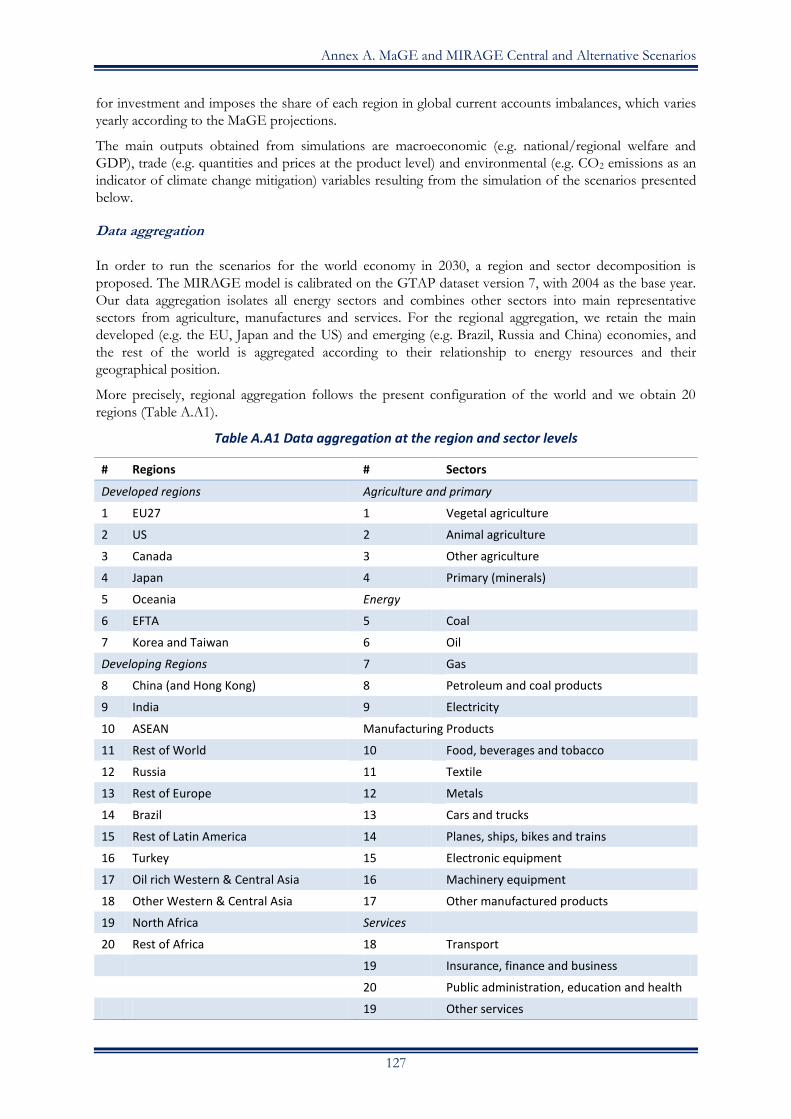
Annex A. MaGE and MIRAGE Central and Alternative Scenarios
127
for investment and imposes the share of each region in global current accounts imbalances, which varies
yearly according to the MaGE projections.
The main outputs obtained from simulations are macroeconomic (e.g. national/regional welfare and
GDP), trade (e.g. quantities and prices at the product level) and environmental (e.g. CO2 emissions as an
indicator of climate change mitigation) variables resulting from the simulation of the scenarios presented
below.
Data aggregation
In order to run the scenarios for the world economy in 2030, a region and sector decomposition is
proposed. The MIRAGE model is calibrated on the GTAP dataset version 7, with 2004 as the base year.
Our data aggregation isolates all energy sectors and combines other sectors into main representative
sectors from agriculture, manufactures and services. For the regional aggregation, we retain the main
developed (e.g. the EU, Japan and the US) and emerging (e.g. Brazil, Russia and China) economies, and
the rest of the world is aggregated according to their relationship to energy resources and their
geographical position.
More precisely, regional aggregation follows the present configuration of the world and we obtain 20
regions (Table A.A1).
Table A.A1 Data aggregation at the region and sector levels
# Regions # Sectors
Developed regions Agriculture and primary
1 EU27 1 Vegetal agriculture
2 US 2 Animal agriculture
3 Canada 3 Other agriculture
4 Japan 4 Primary (minerals)
5 Oceania Energy
6 EFTA 5 Coal
7 Korea and Taiwan 6 Oil
Developing Regions 7 Gas
8 China (and Hong Kong) 8 Petroleum and coal products
9 India 9 Electricity
10 ASEAN Manufacturing Products
11 Rest of World 10 Food, beverages and tobacco
12 Russia 11 Textile
13 Rest of Europe 12 Metals
14 Brazil 13 Cars and trucks
15 Rest of Latin America 14 Planes, ships, bikes and trains
16 Turkey 15 Electronic equipment
17 Oil rich Western & Central Asia 16 Machinery equipment
18 Other Western & Central Asia 17 Other manufactured products
19 North Africa Services
20 Rest of Africa 18 Transport
19 Insurance, finance and business
20 Public administration, education and health
19 Other services
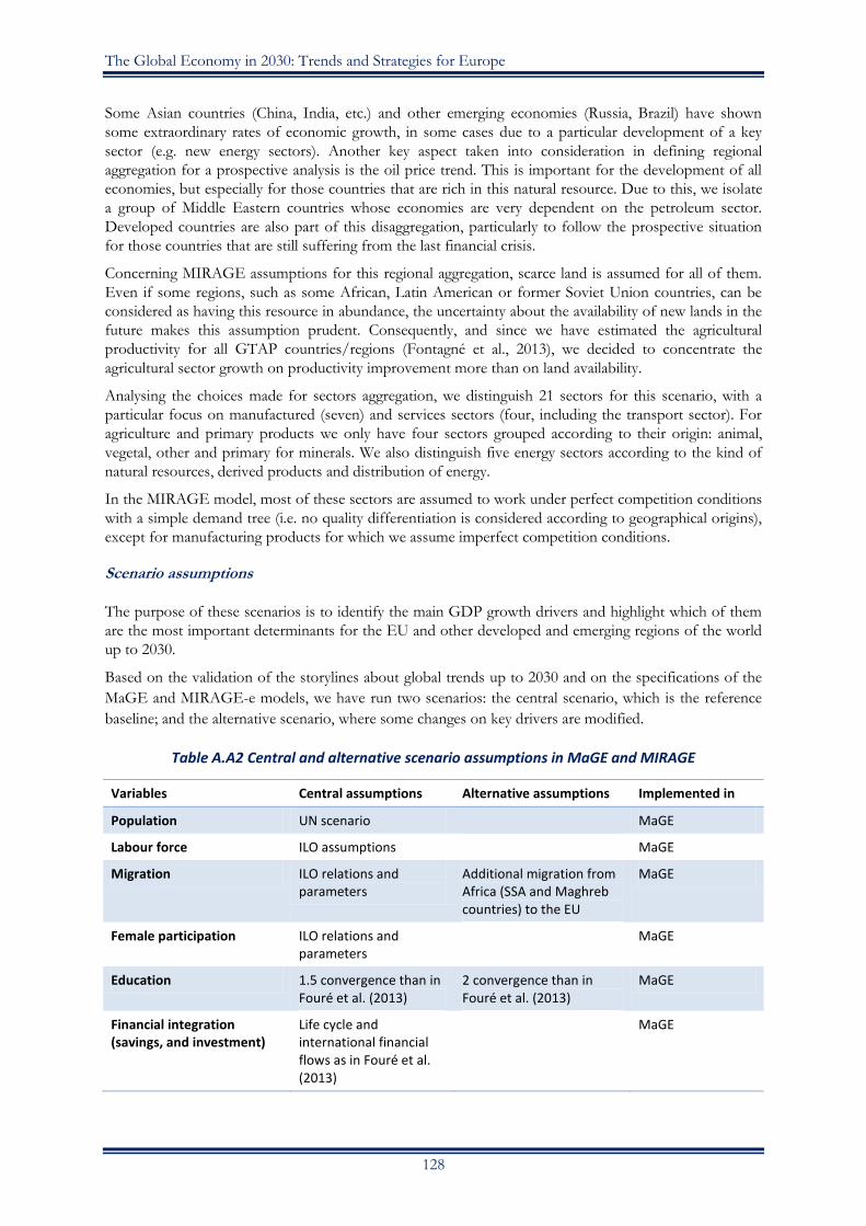
The Global Economy in 2030: Trends and Strategies for Europe
128
Some Asian countries (China, India, etc.) and other emerging economies (Russia, Brazil) have shown
some extraordinary rates of economic growth, in some cases due to a particular development of a key
sector (e.g. new energy sectors). Another key aspect taken into consideration in defining regional
aggregation for a prospective analysis is the oil price trend. This is important for the development of all
economies, but especially for those countries that are rich in this natural resource. Due to this, we isolate
a group of Middle Eastern countries whose economies are very dependent on the petroleum sector.
Developed countries are also part of this disaggregation, particularly to follow the prospective situation
for those countries that are still suffering from the last financial crisis.
Concerning MIRAGE assumptions for this regional aggregation, scarce land is assumed for all of them.
Even if some regions, such as some African, Latin American or former Soviet Union countries, can be
considered as having this resource in abundance, the uncertainty about the availability of new lands in the
future makes this assumption prudent. Consequently, and since we have estimated the agricultural
productivity for all GTAP countries/regions (Fontagné et al., 2013), we decided to concentrate the
agricultural sector growth on productivity improvement more than on land availability.
Analysing the choices made for sectors aggregation, we distinguish 21 sectors for this scenario, with a
particular focus on manufactured (seven) and services sectors (four, including the transport sector). For
agriculture and primary products we only have four sectors grouped according to their origin: animal,
vegetal, other and primary for minerals. We also distinguish five energy sectors according to the kind of
natural resources, derived products and distribution of energy.
In the MIRAGE model, most of these sectors are assumed to work under perfect competition conditions
with a simple demand tree (i.e. no quality differentiation is considered according to geographical origins),
except for manufacturing products for which we assume imperfect competition conditions.
Scenario assumptions
The purpose of these scenarios is to identify the main GDP growth drivers and highlight which of them
are the most important determinants for the EU and other developed and emerging regions of the world
up to 2030.
Based on the validation of the storylines about global trends up to 2030 and on the specifications of the
MaGE and MIRAGE-e models, we have run two scenarios: the central scenario, which is the reference
baseline; and the alternative scenario, where some changes on key drivers are modified.
Table A.A2 Central and alternative scenario assumptions in MaGE and MIRAGE
Variables Central assumptions Alternative assumptions Implemented in
Population UN scenario MaGE
Labour force ILO assumptions MaGE
Migration ILO relations and parameters
Additional migration from Africa (SSA and Maghreb countries) to the EU
MaGE
Female participation ILO relations and parameters
MaGE
Education 1.5 convergence than in Fouré et al. (2013)
2 convergence than in Fouré et al. (2013)
MaGE
Financial integration (savings, and investment)
Life cycle and international financial flows as in Fouré et al. (2013)
MaGE

Annex A. MaGE and MIRAGE Central and Alternative Scenarios
129
Current account Determined by savings and investment dynamics
MaGE
Energy efficiency Projected as in Fouré et al. (2013)
20% higher than results projected in Fouré et al. (2012)
MaGE
TFP growth Catch-up to the leader(s) as in Fouré et al. (2013)
Higher catch-up technology convergence for emerging economies
MaGE
Specific TFP in agriculture DEA on historical data and projections from Fontagné et al. (2013)
MIRAGE
Energy price Central scenario of the IEA
Higher projections MaGE/MIRAGE
Obsolescence 0.06 0.06 MaGE/MIRAGE
Market access (tariffs and NTBs)
No change since their post-Uruguay Round levels (as of 2004)
MIRAGE
Linear cut of 10% in NTBs and trade costs
Linear cut of 20% in NTBs and trade costs
Assumptions for the dynamic reference scenario are mainly implemented within the MaGE model, which
will impact on MIRAGE through the change of some exogenous parameters (GDP growth, population
growth, savings, current account, energy efficiency and female participation in the labour force). Then
CGE-specific assumptions on market access (trade costs, NTBs and tariffs) are also added to the
definition of this reference scenario. All these assumptions are summarised in the following table and
described further.
Concerning the particular assumptions introduced in the MaGE model for the central scenario, population
relies on the UN population scenario and assumes a medium variant for fertility. For labour force, we
include ILO assumptions (relations and parameters of participation), such as for female participation,
for which we extrapolate past trends according to the ILO projections up to 2020.
For the particular case of education, we assume it relies on a catch-up process with geographical country
group-specific speed. Thus, we assume that educational attainment diffuses more to developing countries,
whereas the level in developed countries remains the same. The convergence speed is such that the half-
life time is 1.5 times that of the reference scenario in Fouré et al. (2013).
Concerning financial integration (savings, investment) and current account imbalances, we rely on
the life cycle and international financial flows assumptions such as in Fouré et al. (2013). Investment rate
(as a percentage of GDP) depends on savings through a dynamic error-correction relation. Since savings
are determined by demographic variables, the investment relies on a long-term relationship with savings
to which it tends to converge. Then the savings rate and the resulting current account are imposed on
MIRAGE with a yearly step. In MIRAGE, the capital flows are limited to the compensation of the
current account imbalances.

The Global Economy in 2030: Trends and Strategies for Europe
130
Table A.A3 Average productivity growth in crops and livestock
(percentage point, geometrical means 2010-50)
Region Crops Livestock
Eff. Tech. M Eff. Tech. M
China -0.66 0.66 0.00 0.83 0.22 1.06
Developing Asia -0.80 0.63 -0.17 1.51 0.21 1.72
East and Southeast Asia 0.00 0.52 0.52 0.72 0.24 0.96
Industrial countries -0.79 1.86 1.05 0.39 1.06 1.46
Middle East and North Africa 0.72 0.15 0.87 1.06 0.27 1.33
Central and South America 0.00 0.42 0.42 1.94 0.86 2.82
Sub-Saharan Africa -2.56 1.32 -1.28 0.37 0.22 0.59
Transition economies 1.13 0.87 2.02 0.55 0.90 1.45
US 0.00 2.02 2.02 0.24 1.83 2.07
Source: Fontagné et al. (2013).
In MaGE we also assume that the TFP growth relies on a catch-up process on the leader(s), according to
Fouré et al. (2013). Moreover, since the definition of agricultural production factors is trickier than the
usual ones and technical progress in agriculture seems to be lower than national TFP growth, Fontagné et
al. (2013) estimate and project specific agricultural TFP (by crops and livestock) relying on a data
envelopment analysis (DEA) of historical data. They use the estimated relations to project efficiency
changes while the technical progress growth is set constant at its average value over the past. Table A.A3
shows the projection results including the Malmquist index (M) decomposition (efficiency and
technological changes) for all the considered country groups for the period 2010-50.
World average energy prices are imposed on the model based on the projections by the International
Energy Agency (IEA, 2011) available until 2035. Over the past few years, gas and oil prices have faced
large annual variations. These variations reflect short-term adjustments, which are not related to the
optimal situation computed by MIRAGE and thus, they cannot be handled properly. We therefore
choose to smooth these two price trajectories between 2004 and 2013 such that the model can handle the
general path.
Figure A.A1 Energy price projections, 2004=1, 2004-35
Source: International Energy Agency (2011) and Fontagné et al. (2013) calculations.

Annex A. MaGE and MIRAGE Central and Alternative Scenarios
131
Since no progress is expected in the multilateral arena, tariffs remain at their post-Uruguay Round (2004)
levels. Trade policy data for model calibration are taken from the GTAP database whose source is the
Market Access Maps (MAcMap-HS6) dataset version 2 from CEPII. This dataset assumes the reference
group weighting scheme (Bouët et al., 2008) for the calculation of ad-valorem equivalent tariffs at the
GTAP level of aggregation.
Finally for the central scenario, we assume some progress on non-tariff barriers, thus a reduction of 10%
on trade costs is assumed to be implemented with a linear cut over the whole period. Trade costs in
MIRAGE are modelled as an iceberg trade cost, and the data used to calibrate trade costs are provided by
Minor & Tsigas (2008), who follow the methodology from Hummels & Schaur (2012).
The alternative scenario will be very useful for evaluating potential deviations of main GDP growth drivers
from the central scenario. For this particular study, we thus assume the following changes based on the
initial reference.
Under the alternative scenario we introduce additional migration flows to those imbedded in ILO
scenarios. More precisely, we assume labour force migration from African (SSA and Mediterranean)
countries and the EU. The assumptions behind this are that only the active population migrates, those
migrants keep their qualification of their countries of origin but they take the life expectancy of the host
country.
Compared with the central scenario, we assume a greater speed of convergence of the catch-up process in
education in the alternative scenario. Even if the change in this assumption affects all countries, those
countries that are further from the frontier (middle and low-income countries) will experience a faster
catch-up. The convergence speed under this scenario is such that the half-life time is twice that of the
reference scenario in Fouré et al. (2013).
Another change is the introduction of an exogenous shock on the TFP growth that leads to a higher
speed for emerging economies (20% greater) such as China, justified by the technology transfers.
Remember that the assumptions in the MaGE model are at the country level and since the EU is
composed of high, middle and low-income countries, this change is thus reflected in the EU aggregate
result.
Concerning the energy price, the alternative scenario assumes the higher projection for oil prices, while
in the reference scenario we have assumed the medium projection.
Finally, market access conditions will only be improved through a greater reduction in trade costs (a 20%
reduction) linearly implemented across the period.
132
Annex B. Capital Accumulation in China:
Is overinvestment an issue?
At present, Chinese investment accounts for about 45% of its GDP and there is a significant risk that
maintaining such a high rate will soon lead to a capital overhang. If this happens, China could find itself
in a similar situation to Japan in the 1990s, when investment rates plummeted from a high level, dragging
growth rates down with them.
The fear that China might have overinvested is also based on the observation that their investment rates
over the last ten years have been even higher than those observed in Korea and Japan, at a time when
these countries were also engaged in a very rapid catch-up phase. According to World Bank data, the
investment rate never exceeded 35% of GDP in either country and usually remained close to 30% over
longer periods.
It is difficult to calculate sustainable investment rates. Of course, China is starting with a much lower
capital ratio than advanced countries. Today, the capital stock per worker is still around 13 times higher in
the US than in China (according to World Bank data). Our global model’s simulation predicts that if
China maintains an investment rate of 30% of GDP, the capital stock per worker by 2030 would still be
almost five times higher in the US than it is in China. On the basis of these calculations, therefore, one
might argue that there is little danger of China investing too much. But the capital-to-output ratio, which
measures the productivity of investment, suggests otherwise. Advanced economies typically have a
capital-to-output ratio of between 1.8 and 2.5. In China, this ratio has already reached a value of 2.5,
pointing to signs of excessive investment. Following the assumption of our model that China’s
investment ratio should rapidly fall to 30% of GDP and remain there for roughly the next decade, the
capital-to-output ratio would then rise to about 2.7 in the year 2030, which would indeed be a high value,
but potentially sustainable. If, on the other hand, China were to continue its present investment rate of
45% of GDP (as forecasted by the IMF for the next five years), the capital-to-output-ratio would rise to
above 3.0 by 2030. Under this hypothesis, an important slow-down in investment and hence growth
would thus be likely, even before the value has been reached.
Measurements of capital stock are always fraught with uncertainty, but the major trends determined by
the investment rate are telling. Assuming that the rate of depreciation of capital is 6% per annum, as in
the model, the capital-output ratio would reach an unsustainable level of 3.8 if the Chinese growth rate
were to fall to 6% (as predicted by the model) but the investment rate were to remain at the current level
of 45% of GDP (see Authors’ note, below).
One reason why overinvestment may not be recognised beforehand is that, in the short and medium run,
the dynamics of investment and growth are such that the future growth path can be distorted. The
mechanism through which this happens is the so-called ‘accelerator’: investment is part of aggregate
demand and hence GDP. A higher GDP is associated with higher investment, which also contributes to
capital accumulation and hence increases measured GDP growth. This means that a higher investment
rate seems justified when higher growth rates materialise. This short-run feedback loop makes it very
difficult to estimate the long-run equilibrium growth rate of a country. But what is certain, as suggested by
both theory and historical experience, is that higher investment rates cannot lead to permanently higher
growth rates. The ‘acceleration’ of growth cannot be permanent because once the investment rate reaches
a certain level, returns will start to fall and growth will return to its underlying rate.

Annex B. Capital Accumulation in China
133
Although the potential for this boom-bust cycle is widely recognised, in reality an overinvestment cycle
can arise if the temporary nature of the growth boost from a shock to investment is not taken on board.
This seems to have been the case in China after 2008. The boost to investment driven by government
policies in response to the global slump in demand was extraordinary, in any event. The investment rate
rose from about 41% to 48% of GDP in about three years. This yielded an increase in measured GDP of
several percentage points (as intended since the investment programme was supposed to provide a
stimulus to domestic demand). The problem is that the temporary nature of this investment boom has
not been acknowledged and that growth rates above 10% were taken as a sign that the growth rate of
China had increased, leading to the conclusion that a permanently higher investment rate was appropriate.
In other words, it is just a misperception about the underlying growth rate that seems to make the
combination of permanently higher investment and growth rates sustainable. As long as the capital-
output ratio does not increase, the rate of return on investment will not deteriorate; confirming this
perception. But this cannot go on for long. When the marginal productivity of investment eventually
starts to fall, the boom might have already turned to a bust. At that point, the same ‘accelerator’
mechanism starts to work on the way down: once the capital stock has been recognised as being too high,
a slowdown in investment leads to lower growth, which in turn would seem to make a lower investment
rate appropriate.
This might be happening at present in China, where the stimulus spending has run its course. The
observed growth rates of China in 2008-12 might have been well above the longer-term sustainable rate
and Chinese growth might now undershoot the equilibrium rate for a time until the excess capital
spending of 2009-12 has been absorbed.
The key question is: What are the implications of this behaviour for the rest of the world? To answer this
one needs to know what happens to the savings/investment balance in China, i.e. how the current
account will develop. If China’s national savings rate remains about 50% of GDP, a re-emergence of large
current account surpluses seems unavoidable once the accelerator works in reverse. Under this scenario,
Chinese investment would fall, but since savings do not necessarily follow the same pattern and the
rebalance towards more consumption might not happen, slower growth and large current account
surpluses would be the consequence for the rest of the world.
This potential desire of China to run larger current account surpluses may clash with internal dynamics
occurring within the euro area. The ongoing adjustment in peripheral countries has not been mirrored by
a fall in the surpluses of the core countries so that the euro area is now running a large current account
surplus. It is unlikely that the world economy can stand large current account surplus in two of the largest
world regions.

The Global Economy in 2030: Trends and Strategies for Europe
134
Note: Alternative steady state capital–output ratios
We present below different patterns of capital accumulation based on different hypotheses about
investment and growth rates. The law of motion of the capital-to-output ratio, which describes the
evolution of capital relative to GDP, is described by the following equation:
Where I denote gross investment, g the growth rate of GDP and, in the last part of the equation, it is
assumed that capital depreciates at a rate denoted by δ.
The change in the capital-to-output ratio can thus be written as a function of the investment rate I/Y and
the present capital output ratio:
This implies that one can compute the capital-output ratio at the steady state as a simple ratio:
Assuming δ=6% (0.06 per annum) as in the model, the table below reports the steady state capital-output
ratio for different growth rates.
I/Y
g
0.2 0.25 0.3 0.35 0.4 0.45
0.1 1.9 2.2 2.5 2.8
0.08 1.8 2.1 2.5 2.9 3.2
0.06 1.7 2.1 2.5 2.9 3.3 3.8
0.04 2.0 2.5 3.0 3.5 4.0
0.02 2.5 3.1 3.8 4.4
Source: Author’s elaboration.

135
Annex C. What to expect from TTIP or free trade with a BRIC
nation: The example of India
Transatlantic Trade and Investment Partnership (TTIP)
Trade between the EU and the US has been largely liberalised for a long time. Tariffs are low on both
sides, with a few exceptions in marginal sectors. Non-tariff barriers (NTBs) are thus more important than
the remaining tariffs. These NTBs derive mainly from differences in regulations and standards regarding
industrial products and services to protect consumers. They are more difficult to remove because the
different standards are determined by different preferences, languages and cultures (Ecorys, 2009).
The studies that have been commissioned to quantify the benefits of an agreement along the lines
envisaged in the official documents have generally concluded that the volume of trade will expand
considerably, but that the ultimate welfare gains will remain modest. These studies assume generally that a
TTIP would eliminate all remaining tariffs and non-tariff barriers to trade and that the cost of complying
with regulation would be reduced substantially (typically by about one-fourth). For example, a study by
Ecorys (2009) concludes that “[t]he ambitious scenario could push EU GDP to be 0.7% higher in 2018
compared to the baseline scenario … for the US GDP the same operation yields a 0.3% gain per year in
2018 …”. Another study (CEPR, 2009) finds similar orders of magnitude, i.e. much less than 1% of
GDP.100 Both studies conclude that about 80% of the total gain in welfare would result from the
reduction of NTBs ‘behind the border’. The extent to which these barriers can be reduced depends on
how regulation is formed and applied within both partners. Several sectoral mutual recognition
agreements already exist between the EU and the US, but they have not worked so far in practice because
the regulatory agencies on both sides of the Atlantic concentrate on the pursuit of their own agendas.
Proponents of the TTIP often argue that it would lead to a further strengthening of transatlantic
investment, in particular FDI. The basis of this argument is that the ties in terms of FDI seem to be
much stronger than those in terms of pure trade flows.
The US figures on direct investment abroad101 show that more than half of the reported stock of US FDI
in Europe of $2,300 billion represents holdings of so-called ‘holding companies’, which are often empty
shells and serve mainly to minimise taxes.102 A further 30% is in the ‘finance’ sector, which also often
contains investment vehicles that recycle dividend payments to countries with lower withholding taxes. If
one takes into account the limited relevance of these investments for the real economy, one arrives at a
different picture of the importance of transatlantic FDI. The stock of US investment in firms that
actually produce goods and services might be worth about US$1,000 billion, or 6% of the US economy,
and an even lower percentage of the EU economy. This is not to deny that transatlantic FDI is very
important, but the official figures need to be interpreted with care.
All in all, it therefore appears that even a comprehensive Transatlantic Partnership agreement per se would
not represent a game changer. It is of course possible that the TTIP becomes a template for agreements
100 There is only one other study (by the Bertelsmann Foundation) that finds a much larger impact, almost ten times higher in that the gain is estimated to amount to 9.7% for the UK, 4.7% for Germany and 2.6% for France (and for the US: 13.4%). However, these larger numbers are difficult to accept given that transatlantic trade (goods and services) accounts for about than 2% of GDP on both sides. 101 Eurostat figures give a partially different picture, but this is due to differences in definition and coverage. 102 The Dutch case is particularly illustrative of this phenomenon. It is often reported that US investment in the Netherlands alone is larger than US investment in China. However, the figures for US investment in the Netherlands comprise over 80% investments in these holding companies.
The Global Economy in 2030: Trends and Strategies for Europe
136
with other countries or that a successful TTIP would reinvigorate multilateral trade liberalisation, but
these would be indirect effects that, at present, appear highly uncertain (Mattoo, 2013).
How important would an EU-India free trade agreement be?
By 2030, the working-age population of India will be significantly larger (and younger) than that of China.
It will also be much better educated than today. Could India become the ‘next China’ by 2030? The
economy of India has so far remained rather closed, at least compared with China. One of the reasons
for this is that India still has very high trade barriers, both in terms of tariffs and other non-tariff forms of
protection. The accession of China to the WTO is widely credited as having kick-started the export-
based growth that has allowed the country to grow at double-digit rates over the last 15 years. The
question is now whether a ‘deep’ free trade agreement (FTA) between the EU and India could play a
similar role to WTO membership for China.
The available studies on this topic suggest a negative answer.
In 2007, negotiations for an FTA between the EU and India began. The initiative generated great
expectations due to the potential number of consumers involved; if successful, the agreement would
concern the lives of 1.7 billion people. For this reason the FTA, which is currently being negotiated, is
considered by many policy-makers as a possible game changer for future economic developments.
However, a careful look at the data seems to contradict this. First of all, there is a double-size effect: if it
is true that the potential size of the market is vast, its actual proportion in terms of today’s trade volume is
very limited. The sum of the import and export of goods and services from the EU to India amounted to
€98 billion in 2012,103 representing less than 1% of European aggregate output.
The second reason lies in the fundamental difference between the two economies and their export
sectors, with European manufacturers exporting capital equipment, industrial chemicals, vehicles or
luxury goods that hardly meet the Indian demand.
For these reasons, modelling exercises predict a small impact on growth in Europe should the FTA be
agreed. Using a general equilibrium model (MIRAGE), CEPII-CIREM (2007) predicts that trade
liberalisation would certainly have a positive impact on both sides, but a rather small impact on the EU.104
Along the same lines, the Institute for International and Development Economics (IIDE) (Fillat-
Castejon, 2008) predicts gains for Europe to be in the range of less than 0.1% of GDP, both in the short
and long run. Figures are slightly better on the Indian side: a moderate trade liberalisation, consisting of a
90% reduction in tariffs on goods and 25% in tariffs on services, would increase GDP by 0.1% in the
short run and by 1% in the long run.
However, one should keep in mind that the estimates from China’s WTO membership were also of a
similar order of magnitude. Even in 2002, when China had already become a WTO member, the standard
models predicted that the gains in welfare would be in the order of 0.2% for the world and around 2%
for China itself.
It is thus likely that from a dynamic medium- to long-run perspective, an EU-India FTA could be much
more important than static models based on past data predictions. This does not imply necessarily that
trade liberalisation with the EU would transform India into the next China, but it might mean a much
more dynamic Indian economy, and a large emerging economy with solid democratic traditions much
more closely allied with the EU.
103 See http://ec.europa.eu/trade/policy/countries-and-regions/countries/india/. 104 For completeness, it is necessary to mention that general equilibrium models produce conservative estimates in the sense that they do not take into account productivity and efficiency gains.
Annex C. What to expect from TTIP or free trade with a BRIC nation
137
However, the estimates of the benefits of an EU-India FTA are suggestive of the order of magnitude that
an FTA with China might offer the EU. Given that EU trade with China is about six times as important
as trade with India, the welfare benefits for the EU could well be substantial, even if tariffs are somewhat
lower in the case of China.
138
Annex D. The Results of the NEMESIS Model:
Europe moving towards 2030
Table of Contents
1. Introduction ................................................................................................................................. 139
2. Results for Europe as a whole ...................................................................................................... 140
2.1 Three different growth phases of the period ....................................................................... 140 2.2 The first phase (2011-14): External balance acts as the main driver for GDP ..................... 140 2.3 The second phase (2014-18): The rebound in productivity ................................................. 142 2.4 Third phase (2019-30): Losses in competitiveness .............................................................. 142
3. General overview of the period .................................................................................................... 142
3.1 The drivers of growth ........................................................................................................ 143 3.2 The labour market .............................................................................................................. 143 3.3 Public finances ................................................................................................................... 144 3.4 Sectoral employment .......................................................................................................... 145
4. The results for European countries from NEMESIS runs ............................................................ 146
4.1 Grouping by GDP per capita: Three types of dynamic guided by a certain convergence ..... 146 4.2 Deepening the analysis for the three categories .................................................................. 151
5. Consequences of higher productivity gains ................................................................................... 163
5.1 Calibration, allocation and implementation of the shock .................................................... 163 5.2 Results for the whole of Europe ......................................................................................... 164 5.3 Results for individual European countries .......................................................................... 166
6. Conclusions .................................................................................................................................. 168
Appendix 1. GDP per capita: Levels and average annual growth rates .................................................. 170
Appendix 2. GDP: Levels and average annual growth rates .................................................................. 171
Appendix 3. Population and average annual growth rates of population ............................................... 172
Appendix 4. Some insights on productivity growth .............................................................................. 173
Appendix 5. Results for some European countries ............................................................................... 175
Appendix 6. The NEMESIS Model ...................................................................................................... 185

Annex D. The Results of the NEMESIS Model
139
1. Introduction
This annex presents the results of an exercise based on a simulation using the NEMESIS model for the
27 European countries. Starting mainly with the exogenous variables and drivers as in the CEPII
modelling exercise, we implement model runs and look at the first results. If these are unsatisfactory, or
unrealistic, we make corrections and undertake new simulations. The end outcome is a mix of the model’s
results and corrections based on the modellers’ intuition. The model is econometric and allows for the
implementation of new mechanisms and relationships. It also allows us to describe a ‘non-equilibrium
path’ and the adjustment processes brought on by the major imbalances resulting from the crisis. The
final objective of this exercise is to provide a coherent scenario, based on past trends, for the European
countries up to 2030. It is coherent because it is founded on a detailed accounting framework and
because the main mechanisms are based on econometric work. This scenario will then reveal some
difficulties and challenges that must be faced if there is no implementation of new policies.
The path takes place between the crisis that started in 2008 and the beginning of the labour force decline,
the former bringing about major adjustments: sovereign debt with its consequences on interest rates and
economic growth, labour market disequilibrium and its consequences on wages, etc. One major concern,
when looking to the past, is the evolution of labour productivity; the countries hit hardest by the crisis
were those with the lowest productivity gains prior to 2007. Productivity will therefore be at the core of
our analysis, all the more so because productivity gains after the crisis will not rebound to pre-crisis levels
(around 1.6%). A second concern is ageing and the decline of the labour force in the second phase of the
period. How can the transition towards this demographical stress be managed when the crisis effects fade,
leaving weak unemployment rates for certain countries?
Europe as a whole is made up of very heterogeneous countries in terms of structure, demography,
productivity, economic growth and other criteria. The diagnosis on Europe must therefore be completed
by a more detailed approach to the different countries, which will allow us to classify them into three
categories: the northern European countries with high productivity, the southern European countries
most stricken by crisis and the eastern European countries. Regarding finance, the level of sovereign debt
is a crucial issue in almost all countries, except in some eastern ones, but with relevant differences. This
implies a high level of burden, despite the objective of decreasing public deficits that weigh on public
expenditure. Deleveraging is difficult for some countries that are in a debt trap (high interest rates, less
public expenditure, less growth, less taxation revenues, and so on). Furthermore, the main cause of the
disease in the scenario is linked to productivity gains: after the crisis, the rebound (to 1.3%) will be
insufficient to reach the level of productivity gains before crisis (1.7%). For this reason, we end this report
with what we might call a ‘normative’ exercise. How would the scenario change if we could revert to the
1.7% level, that is to say, if the productivity gains were higher by 0.4% every year? It is a normative
exercise, since we do not describe the measures to be taken in order to reach the 1.7% of productivity
growth, and the productivity shock introduced in the model is exogenous. Nevertheless, we did allocate
these extra productivity gains proportionally to the innovation capacities of the different countries.
The simulation system in the NEMESIS model is composed of 30 productive sectors for each European
country, which determine their macroeconomic growth paths. The aggregation over countries determines
the EU27 sectoral and macroeconomic evolution.
The results will be presented in three parts:
1. The scenario for Europe as a whole 2. The results for European countries from NEMESIS runs 3. Consequences for higher productivity gains
To simplify the presentation, we will first present the results at the EU27 level, then look at the situation
in the individual countries, and finish by presenting a contrasting scenario whereby European countries
succeed in returning to the previous level of productivity gains. Once again, we insist on the spirit of the
exercise: we aim to reflect on whether the results conform to our intuition or, on the contrary, appear
very odd or even a priori false. Most of the time, our intuition prevails in the model results, but
occasionally the opposite occurs. In all cases, we hope the results will give food for thought.

The Global Economy in 2030: Trends and Strategies for Europe
140
2. Results for Europe as a whole
We first present the results for Europe as a whole. We will focus on the macro-dynamics, then give some
insights on the sectoral aspects. What we can see, at a first glance, is that the macro-dynamics of the
period are mainly the result of the interaction between real wage growth and productivity growth, and this
explains the evolution of GDP components and growth.
2.1 Three different growth phases of the period
The three phases are: the competitiveness phase, the rebound in productivity phase and the slowing down
of competitiveness phase.
2.2 The first phase (2011-14): External balance acts as the main driver for GDP
During the first phase, GDP falls and then labour productivity slows down, but after three years of crisis,
unemployment is high and wage growth very low under the productivity gains. Then, Europe increases its
price competitiveness and benefits fully from the resumption in global demand in 2011.
We can see in Figure A.D1 that, despite the slowing down of labour productivity gains, wage growth stays
below productivity growth. In fact, when we look at GDP growth for the period, we can see that it is the
external balance that prevents GDP growth from collapsing and that up to 2014-15, external surpluses are
the main driver for GDP growth (Figure A.D2). The share of consumption in GDP decreases and is
replaced by external surpluses. This is a consequence of wage decreases and of rises in unemployment
that reach a peak of 10.6% in 2013, while the inflation rate is at its lowest level.
Figure A.D1 Labour productivity and real wage growth rates for the EU27, 2010-30
-0.5%
0.0%
0.5%
1.0%
1.5%
2.0%
20
10
20
12
20
14
20
16
20
18
20
20
20
22
20
24
20
26
20
28
20
30
labour productivity
real wage

Annex D. The Results of the NEMESIS Model
141
Figure A.D2 GDP growth rate and contribution of main components to this growth for the EU27,
2010-30
Table A.D1 GDP and components: Level in 2010 and average annual growth rates
2010 (billion € 2005)
2010-15 (%)
2015-20 (%)
2020-25 (%)
2025-30 (%)
GDP 11,504.3 0.85 1.55 1.46 1.39
Private consumption 6,582.1 0.25 1.15 1.47 1.72
Public consumption 2,517.1 0.06 1.03 1.22 1.21
Gross fixed capital formation 2,218.6 0.99 2.82 2.12 1.88
Exports 4,149.0 4.01 3.61 2.61 1.92
Imports 3,885.7 2.93 3.69 2.99 2.51
GDP per capita (K€/cap)* 23,045 23,747 25,379 27,137 28,908
* At the end of the period.
During the first period, government deficits are reduced. However, the debt burden is such that sovereign
debt increases by a significant proportion, as it is a period of low nominal growth (inflation and growth
are very weak). These dynamics of productivity are all explained here by the ‘productivity cycle’; the
second phase starts with the end of this cycle.
Table A.D2 Contributions to GDP growth (in annual average point of GDP growth rate)
Contribution to GDP growth 2010-15 2015-20 2020-25 2025-30
GDP growth 0.85 1.55 1.46 1.39
Private consumption 0.14 0.63 0.80 0.94
Public consumption 0.01 0.21 0.25 0.25
Gross fixed capital formation 0.19 0.56 0.44 0.41
Trade balance 0.51 0.14 -0.04 -0.20
-0.5%
0.0%
0.5%
1.0%
1.5%
2.0%
20
10
20
12
20
14
20
16
20
18
20
20
20
22
20
24
20
26
20
28
20
30
GDP
Private consumption
Investment

The Global Economy in 2030: Trends and Strategies for Europe
142
2.3 The second phase (2014-18): The rebound in productivity
The second period starts with rebounds in productivity and in wages. The productivity rebound is
insufficient to reach the labour productivity growth rate that prevailed before 2007 (1.3% versus 1.7%),
but unemployment is such that wage growth is lower than productivity gains (Figure A.D2).
This lower productivity growth may be due to two phenomena that result from the crisis and the low
GDP growth since 2008: a substitution effect due to weak wages and a slowing down of R&D volume
(although R&D effort – R&D/GDP – is not decreasing) due to GDP stagnation. The low wage is due to
the augmented Phillips curve of the NEMESIS model. The mechanisms linking labour productivity to
factor substitutions, R&D and human capital (skills) are of course reductive, as for all modelling exercises.
Moreover, we assumed that the crisis did not affect the structure of human capital. Nevertheless, we
believe that R&D variations are a major determinant of productivity gains in the long term (see Appendix
3). Throughout the second phase, the growth rate of labour productivity being above the wage curve
allows for the accumulation of price competitiveness gains. With the world demand hypothesis, the
external balance will therefore increase but at a slower pace than in the preceding phase.
GDP growth is then driven simultaneously by internal demand, resulting from a rebound in wages and an
investment catching-up process, as well as by the external balance. GDP growth reaches its highest level
(around +1.62% in 2016) in the first part of this period, but the slack in productivity is reducing, despite a
slight increase in productivity growth, because real wages are increasing faster. There are several possible
explanations for this. Unemployment falls continuously over the period, but we can also consider
(although the mechanism is not present in the model) a contamination of wage increases by the countries
worst hit by crisis. For these reasons, the contribution of external balances to GDP growth decreases
(Table A.D2), and then growth falls at the end of the period. Nevertheless, the share of consumption’s
contribution to GDP decreases in favour of external balances throughout the period in question. The
inflation rate also rebounds, the public deficit decreases and the sovereign debt-to-GDP ratio starts to
decrease very slowly.
2.4 Third phase (2019-30): Losses in competitiveness
The third phase starts when the real wage growth overtakes productivity gains (in 2019). Europe is then
losing price competitiveness, despite slow productivity gains. Falling unemployment increases the real
wage. We can make two main remarks here. The first is on the wage curve used in the model – although
the labour market is far from representing a positive demand excess, wages increase. Many debates have
been conducted previously on the credibility of this description of the labour market, around the
concepts of structural unemployment or of mismatching between supply and demand. Nevertheless, we
believe that this mechanism can lead to a good description of the consequences of a stagnant active
population in an economic area.
The dynamic is very different from that of the two first phases. Although the trade balance still represents
an important part of GDP, its contribution to GDP growth (Table A.D2) soon becomes negative, and
then GDP growth in volume declines until it reaches 1.4% in 2030. This declining GDP growth in
volume is accompanied by slight inflationary pressures, and consequently the GDP growth in value is
increasing faster. For this reason, and also because the deficit reduction policy bears fruit, the debt-to-
GDP ratio is declining faster.
3. General overview of the period
Throughout the period, we examine the evolution of the different disequilibria and restructuring that are
caused by the adjustments resulting from the crisis.

Annex D. The Results of the NEMESIS Model
143
3.1 The drivers of growth
The rebound in labour productivity after the crisis brings productivity growth up the level seen
previously. Several conditions can explain the reduction in R&D that is observed with the NEMESIS
model, as substitution is favourable to labour at the beginning of the period. To this we can add the
difficulties for firms in some countries (Spain, for example) to innovate in a context of weak profit
margins. However, in the countries where the unemployment rate is very high, the only sustainable way to
increase productivity is through product or quality innovation that can create outlets (process innovation
increasing unemployment in the first place). The main drivers for growth are initially external balance, and
then internal demand when real wage growth overtakes productivity gains.
Figure A.D3 Growth rates of GDP, employment and labour productivity for the EU27, 2010-30
3.2 The labour market
The significant disequilibrium at the beginning of the period is progressively reduced and the
unemployment rate reaches 6% at the end (2030). We can see that the fall in unemployment at the end
comes from a reduction in the labour force; the growth cannot create new jobs in 2030.
-1.0%
-0.5%
0.0%
0.5%
1.0%
1.5%
2.0%
20
10
20
11
20
12
20
13
20
14
20
15
20
16
20
17
20
18
20
19
20
20
20
21
20
22
20
23
20
24
20
25
20
26
20
27
20
28
20
29
20
30
GDP
Labour productivity
Employment

The Global Economy in 2030: Trends and Strategies for Europe
144
Figure A.D4 Employment and the labour force in the EU27 (in thousands)
Table A.D3 Evolution of labour in the EU27
µ 2010 2015 2020 2025 2030
Total employment 223,482 224,157 227,411 228,532 229,095
High-skilled 63,377 68,927 76,382 83,677 90,918
Low-skilled 160,106 155,230 151,030 144,855 138,178
Unemployment rate 9.1% 9.7% 8.8% 7.8% 6.1%
Labour force 245,800 248,298 249,339 247,849 244,065
Population 499,201 505,510 510,724 513,428 516,522
In this context of a labour force shortage (Figure A.D4), the figure of 6% unemployment cannot be
considered a good performance for Europe. Moreover, this Europe-wide figure masks widely contrasting
situations. In Germany, low unemployment causes wage increases due to labour shortage that spread
across all sectors and perhaps other countries, whereas Spain is always faced with high unemployment.
For all these reasons, the results are not satisfactory.
3.3 Public finances
The NEMESIS taxation system and accounting framework for agents allow us to compute, for any one
year, the government balance and the gross debt.
In the simulation, we can regulate, in a limited way, the public deficit acting on public expenditures. In a
sense, the reduction of deficits will foster demand in the short term and boost growth (with a lesser debt
burden) over the longer term. We can see that after the measures taken in response to the first (subprime)
crisis, deficit reduction is very difficult during the second (euro) crisis due to the lack of growth and to
very weak inflationary pressures. After the recovery, the deficit-to-GDP reduction could come back to -
3% by around 2020, and the reduction of the deficit is accelerating shortly after until the end of the
period because the slowdown in growth is compensated by slight inflationary pressures. Indeed, this
reveals the difficulty of decreasing the debt-to-GDP ratio in the first part of the period. This global
diagnosis also covers highly heterogeneous evolutions; as we said in the introduction, some countries
could fall in a ‘debt trap’.
205,000
210,000
215,000
220,000
225,000
230,000
235,000
240,000
245,000
250,000
255,000
20
10
20
11
20
12
20
13
20
14
20
15
20
16
20
17
20
18
20
19
20
20
20
21
20
22
20
23
20
24
20
25
20
26
20
27
20
28
20
29
20
30
Labour force
Total Employment

Annex D. The Results of the NEMESIS Model
145
Figure A.D5 Public finance in the EU27, 2010-30
3.4 Sectoral employment
Here, we present the results on sectoral employment for five main sectors. Table A.D4 shows that the
different periods entail different evolutions in the structure of employment.
In the first period up to 2015, the share of industrial employment is constant, meaning that if we take into
account faster productivity gains, the weight of industry in the value added increases, in contrast to the
past. This is the result of the reinforcement of European competitiveness that benefits mainly this sector.
The share of market services employment increases, in accordance with the past. On the other hand,
employment in non-market services is reduced, which is the result of deficit-reduction policies. The share
of agriculture in total employment also decreases, as in the past.
Table A.D4 Shares of total employment by main sectors in EU27
2010 2015 2020 2025 2030
Agriculture 5.40% 4.95% 4.35% 3.81% 3.35%
Industry 16.52% 16.09% 15.24% 14.29% 13.36%
Construction 7.21% 7.60% 8.12% 8.38% 8.50%
Market services 43.02% 44.87% 45.40% 45.56% 45.59%
Non-market services 27.86% 26.49% 26.90% 27.96% 29.20%
For the rest of the period up to 2030, the weight of industrial employment decreases again, to reach only
13% in 2030, due to the loss of competitiveness of the European countries. In contrast, the share of non-
market services in total employment increases for two reasons: the deficit reduction constraint is less
stringent and the ageing population prompts an increase in non-market services such as medical care, and
so on. Moreover, the productivity gains for these sectors are very weak. If the organisation is modified, it
may lead to a change of structural employment. Not surprisingly, the share of agricultural employment
decreases.
74%
76%
78%
80%
82%
84%
86%
88%
90%
92%
20
10
2
01
1
20
12
2
01
3
20
14
2
01
5
20
16
2
01
7
20
18
2
01
9
20
20
2
02
1
20
22
2
02
3
20
24
2
02
5
20
26
2
02
7
20
28
2
02
9
20
30
General government gross debt (% of GDP for EU-27)
-7%
-6%
-5%
-4%
-3%
-2%
-1%
0%
20
10
2
01
1
20
12
2
01
3
20
14
2
01
5
20
16
2
01
7
20
18
2
01
9
20
20
2
02
1
20
22
2
02
3
20
24
2
02
5
20
26
2
02
7
20
28
2
02
9
20
30
General government balance (% of GDP for EU-27)

The Global Economy in 2030: Trends and Strategies for Europe
146
4. The results for European countries from NEMESIS runs
If Europe as a whole encompasses a highly heterogeneous group of countries, we can look for criteria to
categorise the countries and to present all the results in a synthetic way. The first, and simplest idea, is to
use GDP per capita at the beginning (in 2010). We will see that this is a relevant criteria, as it can explain
the future dynamic of countries (perhaps because it is guided by, as we will see, a certain convergence).
4.1 Grouping by GDP per capita: Three types of dynamic guided by a certain
convergence
4.1.1 The characteristics of the three groups
If we look at Figure A.D6, we can see that in 2010, there is a group of northern European countries that
have the highest GDP per capita levels, followed by the southern European countries, and finally the
eastern European countries. Let us go deeper into the characteristics of these countries.
Figure A.D6 GDP per capita in 2010 and average annual growth rate of GDP per capita, 2010-30
Northern Europe (e.g. Germany) was in a better position in terms of competitiveness before the crisis. Its
public balance was less degraded and its trade balance was positive. Northern European economies had
experienced a moderate increase in wages in the years before the crisis, so labour productivity increased at
a higher rate than wages, hence the gain in competitiveness. Although they experienced a severe recession
in 2009, the Nordic countries are in the least dramatic situation among European countries, as they do
not suffer from twin deficits (public accounts and trade balance both in deficit).
Southern Europe (e.g. Spain) had experienced a huge increase in wages, not compensated by a similar
increase in labour productivity, in the decade preceding the crisis. These economies have thus lost
competitiveness and seen a deterioration in their external balance. The dynamism of consumption in
these countries also weighed negatively on their external accounts. Before the crisis, the growth of these
countries relied mainly on strong consumption and growth in investment in housing, and high
0.0%
0.5%
1.0%
1.5%
2.0%
2.5%
3.0%
3.5%
4.0%
4.5%
0 5,000 10,000 15,000 20,000 25,000 30,000 35,000 40,000
Ave
rage
an
nu
al g
row
th r
ate
of
GD
P
GDP per capita in 2010 (€)
Lithuania
Latvia Estonia
Bulgaria Slovakia
Romania Malta
Poland Czech Rep.
Hungary
Sweden Austria
Spain Greece
United Kingdom
Denmark Germany
Belgium
Finland
France
Cyprus Portugal
Italy
Slovenia
Ireland
Netherlands EU27
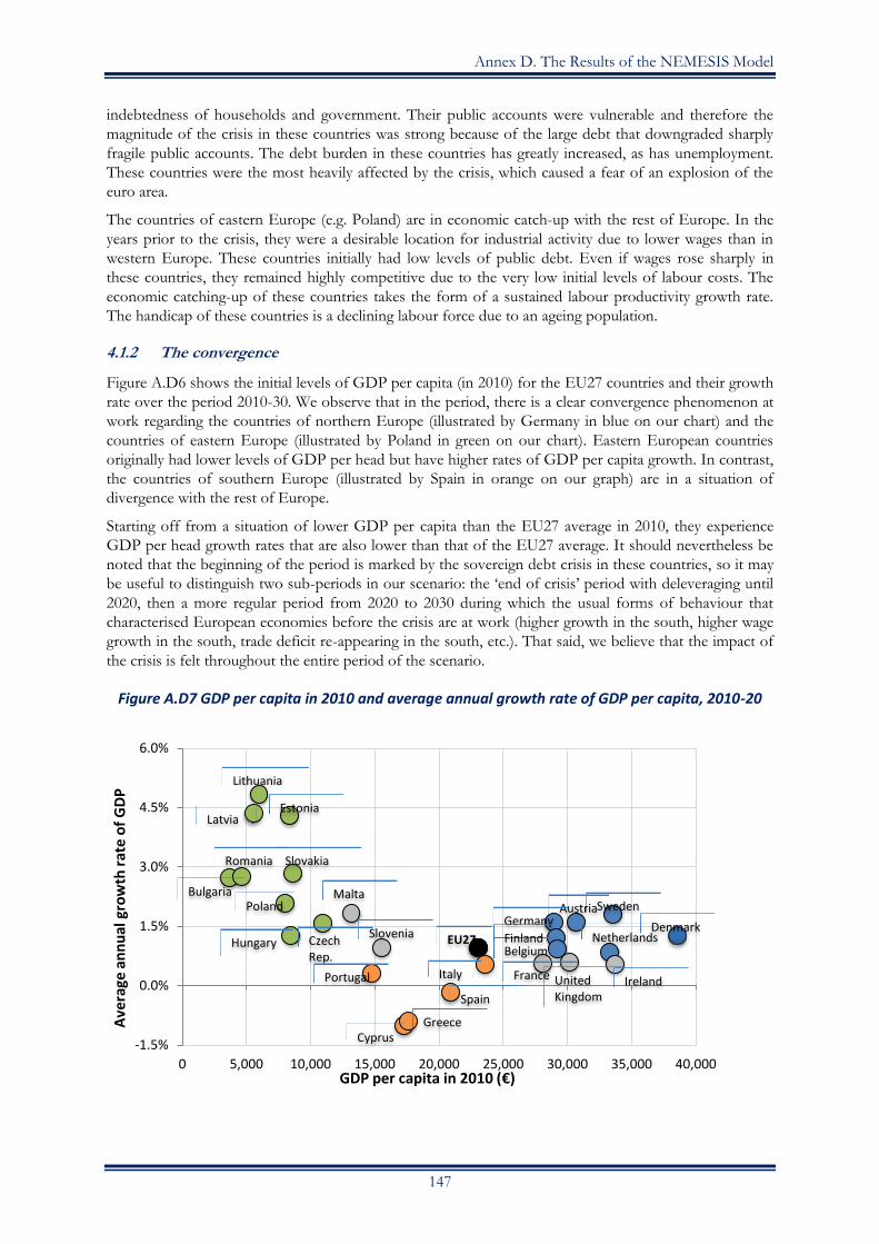
Annex D. The Results of the NEMESIS Model
147
indebtedness of households and government. Their public accounts were vulnerable and therefore the
magnitude of the crisis in these countries was strong because of the large debt that downgraded sharply
fragile public accounts. The debt burden in these countries has greatly increased, as has unemployment.
These countries were the most heavily affected by the crisis, which caused a fear of an explosion of the
euro area.
The countries of eastern Europe (e.g. Poland) are in economic catch-up with the rest of Europe. In the
years prior to the crisis, they were a desirable location for industrial activity due to lower wages than in
western Europe. These countries initially had low levels of public debt. Even if wages rose sharply in
these countries, they remained highly competitive due to the very low initial levels of labour costs. The
economic catching-up of these countries takes the form of a sustained labour productivity growth rate.
The handicap of these countries is a declining labour force due to an ageing population.
4.1.2 The convergence
Figure A.D6 shows the initial levels of GDP per capita (in 2010) for the EU27 countries and their growth
rate over the period 2010-30. We observe that in the period, there is a clear convergence phenomenon at
work regarding the countries of northern Europe (illustrated by Germany in blue on our chart) and the
countries of eastern Europe (illustrated by Poland in green on our chart). Eastern European countries
originally had lower levels of GDP per head but have higher rates of GDP per capita growth. In contrast,
the countries of southern Europe (illustrated by Spain in orange on our graph) are in a situation of
divergence with the rest of Europe.
Starting off from a situation of lower GDP per capita than the EU27 average in 2010, they experience
GDP per head growth rates that are also lower than that of the EU27 average. It should nevertheless be
noted that the beginning of the period is marked by the sovereign debt crisis in these countries, so it may
be useful to distinguish two sub-periods in our scenario: the ‘end of crisis’ period with deleveraging until
2020, then a more regular period from 2020 to 2030 during which the usual forms of behaviour that
characterised European economies before the crisis are at work (higher growth in the south, higher wage
growth in the south, trade deficit re-appearing in the south, etc.). That said, we believe that the impact of
the crisis is felt throughout the entire period of the scenario.
Figure A.D7 GDP per capita in 2010 and average annual growth rate of GDP per capita, 2010-20
-1.5%
0.0%
1.5%
3.0%
4.5%
6.0%
0 5,000 10,000 15,000 20,000 25,000 30,000 35,000 40,000
Ave
rage
an
nu
al g
row
th r
ate
of
GD
P
GDP per capita in 2010 (€)
Lithuania
Latvia Estonia
Bulgaria
Slovakia Romania
Malta Poland
Czech Rep.
Hungary
Sweden Austria
Spain
Greece
United Kingdom
Denmark Germany
Belgium Finland
France
Cyprus
Portugal Italy
Slovenia
Ireland
Netherlands EU27

The Global Economy in 2030: Trends and Strategies for Europe
148
Figure A.D8 GDP per capita in 2020 and average annual growth rate of GDP per capita, 2020-30
Figures A.D8 and A.D9 show the relationship between the level of initial GDP per capita and the growth
rate over the period for the two sub-periods of 2010-20 and 2020-30. We see that, after a decade of
adjustment, deleveraging and deteriorating growth, the southern countries experience more significant
growth rates during the second period (2020-30), providing a relatively complete convergence
phenomenon for the EU27.
To be more precise, the economic growth literature distinguishes two meanings for convergence: ‘sigma-
convergence’ is a reduction in the dispersion of GDP per capita or income levels across economies, while
‘beta-convergence’ occurs when the economies with an initial low income of GDP per capita level grow
faster.
We can test for sigma-convergence by calculating the relative standard deviation of all GDP per capita in
2010, 2020 and 2030 (the ratio of the standard deviation to the average of a data set). We find that there is
indeed a phenomenon of reduced dispersal of GDP per capita over the entire period. In contrast, the
beta-convergence is only observed during the second sub-period (2020-30), as during the first period the
countries of southern Europe have their growth slowed down by the necessary adjustments to their
public accounts.
4.1.3 Does demography explain the differences in growth?
The following graphs detail the relationship between the GDP growth rate and the population growth
rate over the period 2010-30. If we take no account of the difference between the three categories of
country in Europe (as if the colours do not exist), then we can infer from the observation of the set of
points that high population growth is a handicap for the growth of an economy, which is objectively false.
0.0%
0.5%
1.0%
1.5%
2.0%
2.5%
3.0%
3.5%
0 5,000 10,000 15,000 20,000 25,000 30,000 35,000 40,000 45,000
Ave
rage
an
nu
al g
row
th r
ate
of
GD
P
GDP per capita in 2010 (€)
Lithuania
Latvia Estonia
Bulgaria
Slovakia Romania
Malta
Poland Czech Rep.
Hungary
Sweden Austria
Spain
Greece
United Kingdom
Denmark
Germany
Belgium
Finland
France
Cyprus
Portugal
Italy
Slovenia
Ireland Netherlands
EU27

Annex D. The Results of the NEMESIS Model
149
Figure A.D9 Average annual growth rates of GDP and population, 2010-30
The first element is that the growth of the European countries, in green on the chart, is primarily driven
by the catching-up, despite negative population growth (and thus a decreasing labour force). Without the
catching-up phenomenon, these countries would experience very low GDP growth.
We can consider that in the second sub-period, the impact of the declining population begins to be felt
on the growth of these countries.
If we do not include eastern Europe countries in the data set, we instead find a positive relationship
between population growth and GDP growth rates. Of course, this relationship is not perfect, but if
countries like Spain, France or the UK experienced low growth relative to Sweden, Finland and Denmark,
despite their dynamic population, this can easily be explained by the stigma of crisis in these countries.
Demographics do not explain everything.
4.1.4 Slow and incomplete adjustments for unemployment and deleveraging
Figure A.D10 summarises the dynamic adjustment at work in our scenario. The x-axis shows the growth
rate of real wages and the y-axis, the growth rate of labour productivity. The 45° dotted line is the place
where there is a tie between the growth rate of labour productivity and the real wage. Countries above
this line experience higher labour productivity growth than real wage growth, and thus increased
competitiveness. This is the case for the countries of southern Europe, like Spain. Countries below this
line lose competitiveness as growth in real wages is higher than that in labour productivity. This is the
case of countries of northern Europe, like Germany. The countries of eastern Europe are experiencing
strong growth in labour productivity (catching-up), which offsets the dynamic growth in real wages over
the period.
0.0%
0.5%
1.0%
1.5%
2.0%
2.5%
3.0%
3.5%
4.0%
-1.0% -0.5% 0.0% 0.5% 1.0%
Ave
rage
an
nu
al g
row
th r
ate
of
GD
P
Average annual growth rate of population
Lithuania
Latvia
Estonia
Bulgaria
Slovakia
Romania
Malta
Poland
Czech Rep.
Hungary
Sweden
Austria
Spain
Greece
United Kingdom
Denmark
Germany
Belgium
Finland
France
Cyprus
Portugal Italy
Slovenia
Ireland
Netherlands EU27

The Global Economy in 2030: Trends and Strategies for Europe
150
Figure A.D10 Average annual growth rate of labour productivity and real wages, 2010-30
One of the most striking elements of our scenario is the incompleteness of the adjustment in reducing
unemployment and public debt by the end of the period.
Starting from an initial situation in which some of the eastern European countries have high levels of
unemployment and some of the countries of southern Europe have high levels of public debt (the
countries of northern Europe being in an intermediate situation), we find that the eastern European
countries are able to reduce their levels of unemployment, while the northern Europe countries both
lower their level of unemployment (sometimes helped by the reduction of their labour force) and the
weight of their debt. However, southern European countries reduce their unemployment very little over
the period and the weight of their debt stabilises at best, but does not drop.
0.0%
0.5%
1.0%
1.5%
2.0%
2.5%
3.0%
3.5%
4.0%
-0.5% 0.0% 0.5% 1.0% 1.5% 2.0% 2.5% 3.0% 3.5% 4.0%
Ave
rage
an
nu
al g
row
th r
ate
of
lab
ou
r p
rod
uct
ivit
y
Average annual growth rate of real wage
Lithuania
Latvia
Estonia
Bulgaria
Slovakia Romania
Malta Poland
Czech Rep.
Hungary
Sweden Austri
a
Spain Greece
United Kingdom
Denmark Germany
Belgium
Finland
France
Cyprus
Portugal
Italy
Slovenia
Ireland
Netherlands EU27

Annex D. The Results of the NEMESIS Model
151
Figure A.D11 Unemployment rate and public debt as percentage of GDP in 2010
Figure A.D12 Unemployment rate and public debt as percentage of GDP in 2030
4.2 Deepening the analysis for the three categories
Having roughly characterised the main features of the three groups of countries, we now want to deepen
the analysis. Instead of an exhaustive analysis of all countries, we will focus on three countries, each
seeming to us representative of one of the three groups: Germany for the northern European countries,
Spain for the southern European countries, and Poland of course for the eastern European countries. In
each presentation, we will, as for Europe, first explain the components of growth by productivity and real
0%
20%
40%
60%
80%
100%
120%
140%
160%
0% 5% 10% 15% 20% 25%
Pu
blic
deb
t as
% o
f G
DP
Unemployment rate
Greece
Cyprus
Portugal
Italy
Estonia
Ireland
Belgium
Germany
Hungary
Denmark Sweden
Bulgaria
Netherlands
Czech Rep.
Slovakia
Finland
Slovenia Latvia
Lithuania
Romania
Poland
Austria EU27 UK
France
Malta
Spain
0%
20%
40%
60%
80%
100%
120%
140%
160%
0% 5% 10% 15% 20% 25%
Pu
blic
de
bt
as %
of
GD
P
Unemployment rate
Greece
Cyprus
Portugal
Italy
Ireland Belgium
Germany
Hungary
Denmark
Sweden Bulgaria
Netherlands
Czech Rep.
SK
Slovenia
Latvia
Lithuania
Romania
Poland Austria
EU27
UK France
Malta
Spain
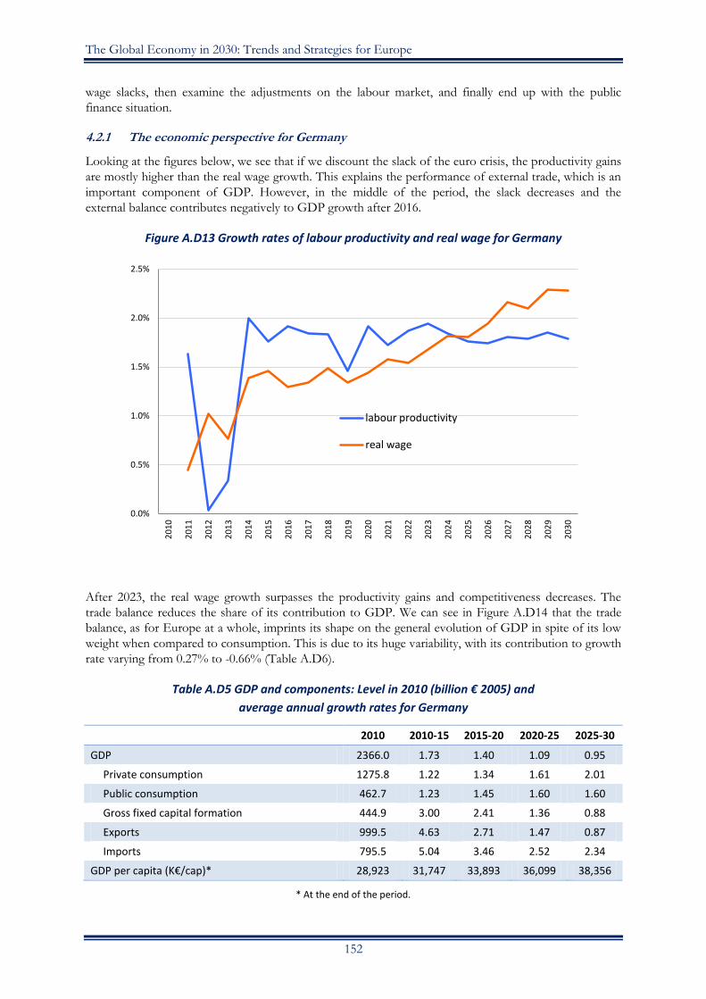
The Global Economy in 2030: Trends and Strategies for Europe
152
wage slacks, then examine the adjustments on the labour market, and finally end up with the public
finance situation.
4.2.1 The economic perspective for Germany
Looking at the figures below, we see that if we discount the slack of the euro crisis, the productivity gains
are mostly higher than the real wage growth. This explains the performance of external trade, which is an
important component of GDP. However, in the middle of the period, the slack decreases and the
external balance contributes negatively to GDP growth after 2016.
Figure A.D13 Growth rates of labour productivity and real wage for Germany
After 2023, the real wage growth surpasses the productivity gains and competitiveness decreases. The
trade balance reduces the share of its contribution to GDP. We can see in Figure A.D14 that the trade
balance, as for Europe at a whole, imprints its shape on the general evolution of GDP in spite of its low
weight when compared to consumption. This is due to its huge variability, with its contribution to growth
rate varying from 0.27% to -0.66% (Table A.D6).
Table A.D5 GDP and components: Level in 2010 (billion € 2005) and
average annual growth rates for Germany
2010 2010-15 2015-20 2020-25 2025-30
GDP 2366.0 1.73 1.40 1.09 0.95
Private consumption 1275.8 1.22 1.34 1.61 2.01
Public consumption 462.7 1.23 1.45 1.60 1.60
Gross fixed capital formation 444.9 3.00 2.41 1.36 0.88
Exports 999.5 4.63 2.71 1.47 0.87
Imports 795.5 5.04 3.46 2.52 2.34
GDP per capita (K€/cap)* 28,923 31,747 33,893 36,099 38,356
* At the end of the period.
0.0%
0.5%
1.0%
1.5%
2.0%
2.5%
20
10
20
11
20
12
20
13
20
14
20
15
20
16
20
17
20
18
20
19
20
20
20
21
20
22
20
23
20
24
20
25
20
26
20
27
20
28
20
29
20
30
labour productivity
real wage

Annex D. The Results of the NEMESIS Model
153
Figure A.D14 GDP growth rate and contributions of main components to the growth of GDP
for Germany, 2010-30
To sum up, we can say that in spite of high productivity gains in Germany – well above the mean for
Europe – real wage growth is higher because tensions appear in the labour market. Then, growth is
towards the end essentially driven by consumption, and declines to 0.97% in 2030.
Table A.D6 GDP growth and contributions to GDP growth
(annual average point of GDP growth rate)
2010-15 2015-20 2020-25 2025-30
GDP growth 1.73 1.40 1.09 0.95
Private consumption 0.65 0.70 0.85 1.11
Public consumption 0.24 0.28 0.31 0.32
Gross fixed capital formation 0.58 0.49 0.29 0.19
Trade balance 0.27 -0.07 -0.36 -0.66
We can observe on the simulation horizon the increasing contribution of final consumption to GDP
growth, and the diminishing contribution to GDP of the trade balance. Although the trade balance
remains positive until 2030, its contribution to the GDP growth decreases gradually from 2011 to 2030,
becoming negative in 2017 onwards (with an exception in 2019), provoking a gradual reduction of the
GDP growth rate over the whole period.
This increase in real wages comes from a labour scarcity and then tensions that appear progressively in
the labour market. We can see in Figure A.D15 that the labour force declines very early on in the period.
Unemployment falls to 2.9% in 2030. We can also see that if unemployment is reduced, the GDP growth
is insufficient to increase employment, taking into account the productivity gains. However, this decrease
in employment does not strike equally across all skills. High-skilled employment continues to increase,
while low-skilled is decreasing rather quickly at the end (Table A.D7).
-1.0%
-0.5%
0.0%
0.5%
1.0%
1.5%
2.0%
2.5%
3.0%
3.5% 2
01
0
20
11
20
12
20
13
20
14
20
15
20
16
20
17
20
18
20
19
20
20
20
21
20
22
20
23
20
24
20
25
20
26
20
27
20
28
20
29
20
30
GDP
Private consumption
Investment
Public consumption
Trade Balance

The Global Economy in 2030: Trends and Strategies for Europe
154
Figure A.D15 Employment and labour force in Germany, 2010-30
Table A.D7 Employment (in thousands) in Germany
2010 2015 2020 2025 2030
Total Employment 40,477 41,655 40,845 39,377 37,771
High-skilled 11,429 12,510 13,048 13,285 13,334
Low-skilled 29,048 29,145 27,797 26,092 24,437
Unemployment rate 7.0% 4.8% 4.7% 4.4% 2.9%
Labour force 43,521 43,741 42,878 41,172 38,907
Population 81,802 81,206 81,529 80,800 79,718
The evolution of employment is very different for the different sectors. The share of agriculture is
declining but what is striking is the decrease of industrial employment, at a slow pace at the beginning and
more quickly at the end. This corresponds to the competitiveness losses for Germany that increase at the
end of the period – industry manufactures relatively more traded products. The share of employment lost
by industry is compensated by that of non-market services.
Table A.D8 Shares of total employment by main sectors in Germany
2010 2015 2020 2025 2030
Agriculture 2.06% 1.81% 1.56% 1.34% 1.14%
Industry 19.41% 18.21% 16.57% 14.74% 12.82%
Construction 5.62% 6.25% 6.64% 6.75% 6.67%
Market services 44.22% 44.97% 44.23% 42.83% 41.03%
Non-market services 28.69% 28.77% 30.99% 34.34% 38.34%
Public finances seem to not be a problem for Germany. The government’s primary balance will soon be
positive (in 2015), as seen in Table A.D9. If the general government balance remains negative, its rate of
1% is lower than the rate of growth in value, then the general government gross debt as % of GDP is
decreasing. At the end, the deleveraging is accelerated because if the growth rate in volume decelerates,
inflationary pressures compensate largely the slowing down. In 2030, the debt represents 48.4% of GDP.
34,000
35,000
36,000
37,000
38,000
39,000
40,000
41,000
42,000
43,000
44,000
45,000
20
10
20
11
20
12
20
13
20
14
20
15
20
16
20
17
20
18
20
19
20
20
20
21
20
22
20
23
20
24
20
25
20
26
20
27
20
28
20
29
20
30
Labour force
Total Employment

Annex D. The Results of the NEMESIS Model
155
Table A.D9 Public finances in Germany (in billion € 2005 and % of GDP)
Public finance (in billion €) 2010 2015 2020 2025 2030
General government balance -102.4 -26.2 -23.8 -12.4 50.4
General government balance (% GDP) -4.3% -0.9% -0.7% -0.3% 1.1%
Government primary balance -42.9 43.9 58.8 80.3 145.0
Government primary balance (% GDP) -2% 1.5% 1.7% 2.0% 3.0%
General government gross debt 1976.7 2210 2317 2415 2313
General government gross debt (% GDP) 83.0% 75.6% 67.1% 59.5% 48.4%
Figure A.D16 General government gross debt and public balance for Germany (% of GDP)
4.2.2 The economic perspective for Spain
The beginning of the period (2010-13) is marked by a deep recession and negative growth in both GDP
and employment. The adjustment in employment is more significant than that of GDP, so that during the
recession years, the growth of labour productivity remains above 1%. Then a second period begins during
which the impact of the crisis (high unemployment levels) paves the way for the Spanish economy to
restart based on competitiveness gains enabled by low wages. The difference between the growth rates of
labour productivity and real wage is 2 points in 2015 and slowly decreases until 2020, when it is still 1
point. The growth of labour productivity is low enough so that the real wage growth is negative from
2015 to 2020. With Spain therefore experiencing significant competitiveness gains, the contribution of
foreign trade to growth is high. For the period 2010-15, GDP decreases 0.6% per year on average, and it
would decrease 2.2% per year without the important contribution of the current account balance to GDP
over the period: 1.6% per year. For the next period 2015-20, the contribution of external balance to GDP
stays very high, at 0.9% per year, accounting for more than 50% of the annual average GDP growth rate
of 1.4%.
0%
10%
20%
30%
40%
50%
60%
70%
80%
90%
20
10
2
01
1
20
12
2
01
3
20
14
2
01
5
20
16
2
01
7
20
18
2
01
9
20
20
2
02
1
20
22
2
02
3
20
24
2
02
5
20
26
2
02
7
20
28
2
02
9
20
30
General government gross debt
-5%
-4%
-3%
-2%
-1%
0%
1%
2%
20
10
2
01
1
20
12
2
01
3
20
14
2
01
5
20
16
2
01
7
20
18
2
01
9
20
20
2
02
1
20
22
2
02
3
20
24
2
02
5
20
26
2
02
7
20
28
2
02
9
20
30
General government balance

The Global Economy in 2030: Trends and Strategies for Europe
156
Figure A.D17 Growth rates of labour productivity and real wage for Spain
Table A.D10 GDP for Spain and its components: Level in 2010 (in € billion 2005) and
average annual growth rates
2010 2010-15 2015-20 2020-25 2025-30
GDP 960.0 -0.58 1.39 1.63 1.76
Private consumption 557.0 -1.38 0.14 1.09 1.82
Public consumption 201.1 -2.24 0.39 0.18 0.43
Gross fixed capital formation 231.8 -4.06 1.85 2.66 3.89
Exports 207.4 5.21 5.18 3.93 2.61
Imports 241.0 -1.25 2.95 3.50 3.82
GDP per capita (K€/cap)* 20,875 19,601 20,535 21,913 23,667
* At the end of the period.
Thus the growth is mainly driven by external demand addressed to Spain, which is strong given the huge
reduction of costs. This competitiveness is mainly based on prices, and the level of investments (and of
R&D) is insufficient to generate non-price competitiveness gains. At the beginning, investment is rather
low but increases throughout the period, due to a structural effect. Improving competitiveness leads to a
reversal of the trends at work earlier. The share of industry in GDP grows again so that more capital-
intensive sectors lead to an increase in the investment rate of the economy. However, given the low wage
growth, labour productivity is not growing at a pace that suggests this significant level of investment. The
capital growth will perhaps not immediately increase labour productivity, because the high unemployment
rate may prompt policy measures that weigh on productivity.
-1.5%
-1.0%
-0.5%
0.0%
0.5%
1.0%
1.5%
2.0%
2.5%
20
10
20
11
20
12
20
13
20
14
20
15
20
16
20
17
20
18
20
19
20
20
20
21
20
22
20
23
20
24
20
25
20
26
20
27
20
28
20
29
20
30
labour productivity
real wage

Annex D. The Results of the NEMESIS Model
157
Figure A.D18 GDP growth rate for Spain and contributions of main components to
the growth of GDP, 2010-30
The very low growth in public spending over the period (in order to restore public finances, which had
deteriorated at the very beginning of the period) and the loss of purchasing power of households, which
weighs on growth in private consumption, led to very low growth in domestic demand (the growth rate is
even negative until 2015). As a result, despite the gains in competitiveness and the slight increase of
growth driven by improvements in foreign trade, GDP grows by an average of only 1.39% per year
between 2015 and 2020, and by 1.7% between 2020 and 2030. However, the increase in GDP, in a
context of a strong rise in the labour force, is not sufficient to significantly reduce unemployment. We
will discuss this in the next section on the labour market.
During the latter part of the scenario (beyond 2020), private consumption is again the main driver of
GDP growth in Spain. At the very end of the period, real wage growth rises above that of labour
productivity. This allows the growth rate of GDP to continue its acceleration (1.63% on average in 2020-
25, 1.76% in 2025-30). The contribution of foreign trade becomes slightly negative.
Table A.D11 Contribution to GDP growth for Spain in annual average point of GDP growth rate
2010-15 2015-20 2020-25 2025-30
GDP -0.58 1.39 1.63 1.76
Private consumption -0.79 0.07 0.57 0.93
Public consumption -0.45 0.07 0.03 0.07
Gross fixed capital formation -0.91 0.38 0.56 0.88
Trade balance 1.58 0.87 0.47 -0.12
The dynamic in Spain throughout the period is based mainly on the trade balance up to 2020 and, after
2020, the contribution of the trade balance to GDP growth remains important. The unemployment rate
stays very high between 2020 and 2030, and this places a high pressure on wages, which explains the
durability of the external competitiveness of Spain until 2025.
-3.0%
-2.5%
-2.0%
-1.5%
-1.0%
-0.5%
0.0%
0.5%
1.0%
1.5%
2.0%
2.5% 2
01
0
20
11
20
12
20
13
20
14
20
15
20
16
20
17
20
18
20
19
20
20
20
21
20
22
20
23
20
24
20
25
20
26
20
27
20
28
20
29
20
30
GDP
Private consumption
Investment
Public consumption
Trade Balance

The Global Economy in 2030: Trends and Strategies for Europe
158
Spain is one of the countries that has been most affected by crisis. The unemployment rate rose to 25%
after 2010 and this high level continues throughout the first period of the scenario (24.6% in 2015 and
24.1% in 2020). Consequently, the growth rate of wages falls and, even if the inflationary pressure is low
(inflation rate between 1% and 1.5%), the growth rate of real wage is negative until 2020.
Figure A.D19 Employment and labour force in Spain, 2010-30
Table A.D12 Employment in Spain (in thousands)
Employment 2010 2015 2020 2025 2030
Total employment 18,674 17,328 17,927 18,841 20,196
High-skilled 6,687 6,637 7,473 8,484 9,777
Low-skilled 11,987 10,690 10,454 10,357 10,419
Unemployment rate 20.1% 24.6% 24.1% 21.9% 17.1%
Labour force 23,370 22,983 23,617 24,121 24,349
Population 45,989 47,570 48,649 49,420 49,928
This advantage in terms of labour costs could lead Spain to specialise in labour-intensive production and
could be one of the explanations for the low growth in labour productivity (structural effect). Moreover,
Spain is experiencing a sustained growth of its labour force. This explains why, despite the rather high
pace of job creation from 2014, unemployment decreases very slowly. The unemployment rate at the end
of the period (2030) stays very high, at about 17%, and it continues to exert high pressure on the hourly
wage.
Table A.D13 Shares of total employment by main sectors in Spain
2010 2015 2020 2025 2030
Agriculture 4.34% 4.19% 3.79% 3.46% 3.12%
Industry 13.80% 15.01% 15.54% 15.83% 15.65%
Construction 9.51% 9.03% 9.17% 9.41% 9.99%
Market services 41.90% 44.15% 45.19% 46.75% 48.44%
Non-market services 30.45% 27.61% 26.31% 24.55% 22.80%
15,000
16,000
17,000
18,000
19,000
20,000
21,000
22,000
23,000
24,000
25,000
20
10
20
11
20
12
20
13
20
14
20
15
20
16
20
17
20
18
20
19
20
20
20
21
20
22
20
23
20
24
20
25
20
26
20
27
20
28
20
29
20
30
Labour force
Total Employment

Annex D. The Results of the NEMESIS Model
159
If we look at the structure of employment (Table A.D13), we can see that unlike most of the other
European countries, the share of industrial employment increases over the period. This is mainly due to
the competitiveness gains resulting from the falling wages. We can see also that public finance constraints
weigh on the non-market services employment, and that unskilled employment decreases while skilled
jobs increase.
Throughout the whole scenario period, the rate of growth of public spending in real terms is almost zero.
However, with the high level of sovereign debt after the crisis and the lack of growth in GDP, the ratio of
public debt to GDP continues to grow until the mid-2020s.
Table A.D14 Public finances in Spain (in billion € 2005 and in % of GDP)
2010 2015 2020 2025 2030
General government balance -96.4 -69.7 -79.4 -65.4 -36.0
General government balance (% GDP) -9.2% -6.2% -6.2% -4.4% -2.0%
Government primary balance -76.5 -30.8 -20.7 10.1 50.8
Government primary balance (% GDP) -7% -2.7% -1.6% 0.7% 2.9%
General government gross debt 641.2 1,022 1,416 1,775 2,022
General government gross debt (% GDP) 61.2% 90.9% 111.3% 119.9% 114.9%
Figure A.D20 General government gross debt and public balance for Spain (% of GDP), 2010-30
4.2.3 The economic perspective for Poland
The main characteristic of the eastern European countries is high productivity gains due to a
redeployment of economic activities towards those with more productivity and to a catching-up effect
with western European countries. These gains allow substantial wage increases, although inferior to
productivity gains (Figure A.D21).
0%
20%
40%
60%
80%
100%
120%
140%
20
10
2
01
1
20
12
2
01
3
20
14
2
01
5
20
16
2
01
7
20
18
2
01
9
20
20
2
02
1
20
22
2
02
3
20
24
2
02
5
20
26
2
02
7
20
28
2
02
9
20
30
General government gross debt
-10%
-9%
-8%
-7%
-6%
-5%
-4%
-3%
-2%
-1%
0%
20
10
2
01
1
20
12
2
01
3
20
14
2
01
5
20
16
2
01
7
20
18
2
01
9
20
20
2
02
1
20
22
2
02
3
20
24
2
02
5
20
26
2
02
7
20
28
2
02
9
20
30
General government balance
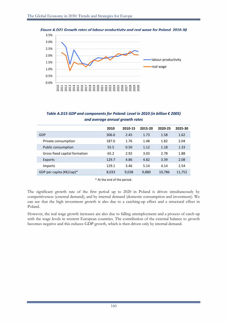
The Global Economy in 2030: Trends and Strategies for Europe
160
Figure A.D21 Growth rates of labour productivity and real wage for Poland, 2010-30
Table A.D15 GDP and components for Poland: Level in 2010 (in billion € 2005)
and average annual growth rates
2010 2010-15 2015-20 2020-25 2025-30
GDP 306.6 2.45 1.73 1.58 1.62
Private consumption 187.6 1.76 1.48 1.82 2.04
Public consumption 55.5 0.50 1.12 1.18 1.33
Gross fixed capital formation 65.2 2.92 3.03 2.78 1.88
Exports 129.7 4.86 4.82 3.39 2.08
Imports 129.1 3.46 5.14 4.14 2.54
GDP per capita (K€/cap)* 8,033 9,038 9,880 10,786 11,752
* At the end of the period.
The significant growth rate of the first period up to 2020 in Poland is driven simultaneously by
competitiveness (external demand), and by internal demand (domestic consumption and investment). We
can see that the high investment growth is also due to a catching-up effect and a structural effect in
Poland.
However, the real wage growth increases are also due to falling unemployment and a process of catch-up
with the wage levels in western European countries. The contribution of the external balance to growth
becomes negative and this reduces GDP growth, which is then driven only by internal demand.
0.0%
0.5%
1.0%
1.5%
2.0%
2.5%
3.0%
3.5%
20
10
2
01
1
20
12
2
01
3
20
14
2
01
5
20
16
2
01
7
20
18
2
01
9
20
20
2
02
1
20
22
2
02
3
20
24
2
02
5
20
26
2
02
7
20
28
2
02
9
20
30
labour productivity
real wage

Annex D. The Results of the NEMESIS Model
161
Figure A.D22 GDP growth rate for Poland and contributions of main components to
the growth of GDP, 2010-30
Table A.D16 GDP growth and contribution to GDP growth
(annual average point of GDP growth rate)
2010-15 2015-20 2020-25 2025-30
GDP growth 2.45 1.73 1.58 1.62
Private consumption 1.07 0.87 1.07 1.22
Public consumption 0.08 0.18 0.19 0.21
Gross fixed capital formation 0.64 0.68 0.66 0.47
Trade balance 0.67 0.01 -0.33 -0.26
The labour market at the beginning is impacted by the crisis, but also by a strong increase in the labour
force. The unemployment rate subsequently reaches 10% in 2015. However, soon thereafter, the labour
force reduction decreases unemployment and therefore the real wage growth will reach that of
productivity gains. We can see in Figure A.D23 how the declining labour force modifies unemployment.
We see also in Table A.D17 that it is only the low-skilled jobs that fall at the end of the period.
-1%
0%
1%
2%
3%
4%
5%
20
10
20
11
20
12
20
13
20
14
20
15
20
16
20
17
20
18
20
19
20
20
20
21
20
22
20
23
20
24
20
25
20
26
20
27
20
28
20
29
20
30
GDP
Private consumption
Investment
Public consumption
Trade Balance

The Global Economy in 2030: Trends and Strategies for Europe
162
Figure A.D23 Employment and labour force in Poland, 2010-30
Table A.D17 Employment in Poland (in thousands)
2010 2015 2020 2025 2030
Total Employment 15,867 16,001 16,168 15,937 15,488
High-skilled 4,028 4,564 5,248 5,843 6,344
Low-skilled 11,839 11,437 10,920 10,093 9,144
Unemployment rate 7.7% 9.9% 7.1% 5.6% 5.3%
Labour force 17,196 17,762 17,400 16,879 16,348
Population 38,167 38,279 38,162 37,806 37,610
When we look at the future of structural employment for Poland, we can see that the net decline of
agriculture and industry at the end of the period is the result of weakened competitiveness
Table A.D18 Shares of total employment in Poland by main sectors
2010 2015 2020 2025 2030
Agriculture 13.17% 12.07% 10.64% 9.30% 8.11%
Industry 22.00% 19.52% 17.47% 15.55% 13.95%
Construction 8.09% 8.57% 8.94% 9.01% 8.60%
Market services 33.95% 37.27% 39.74% 41.54% 42.70%
Non-market services 22.80% 22.56% 23.21% 24.60% 26.65%
Public debt in Poland increases until 2020 and then decreases slightly as the general government balance
tends to zero.
14,000
14,500
15,000
15,500
16,000
16,500
17,000
17,500
18,000
18,500
20
10
20
11
20
12
20
13
20
14
20
15
20
16
20
17
20
18
20
19
20
20
20
21
20
22
20
23
20
24
20
25
20
26
20
27
20
28
20
29
20
30
Labour force
Total Employment

Annex D. The Results of the NEMESIS Model
163
Table A.D19 Public finances in Poland (in billion € 2005 and % of GDP)
Public finance (in billion €) 2010 2015 2020 2025 2030
General government balance -23.3 -15.8 -14.1 -8.9 0.0
General government balance (% GDP) -7.9% -4.0% -2.8% -1.4% 0.0%
Government primary balance -15.4 -3.7 2.2 10.2 19.6
Government primary balance (% GDP) -5% -0.9% 0.4% 1.6% 2.5%
General government gross debt 161.9 245 321 377 396
General government gross debt (% GDP) 54.8% 61.9% 64.6% 60.9% 51.3%
Figure A.D24 General government gross debt and public balance for Poland (% of GDP), 2010-30
5. Consequences of higher productivity gains
We have seen that, despite a significant reduction of unemployment to 6% in 2030, this Europe-wide
result is not satisfactory because it covers very different situations. We saw also that at the end of the
period, the main disease in Europe is decreasing competitiveness. Finally, the rebound of productivity is
not sufficiently high to catch up with past performance. Taking into account the essential role of
productivity in our analysis and the uncertainty of its computing, we perform a sensitivity analysis on it.
More precisely, we try to run the NEMESIS model to respond to the following question: What would be
the consequences of a catching-up of productivity? That is to say, an increase in productivity gains from
1.3% to 1.6-1.7% every year.
First, we describe the methodology used to implement the shock of productivity. Then we will present
the results for Europe as a whole and for some countries of the types that we described earlier. Finally,
we will present some new views on ways of increasing productivity.
5.1 Calibration, allocation and implementation of the shock
Labour productivity is, in the model, a result of the simulations, but it can be influenced by the
introduction of an exogenous shock in the supply block of the model. At first, we introduced a shock that
will increase labour productivity by about 0.4% per year and cumulative gains of 8% for the whole period
2014-30 to reach, for the whole of Europe, the productivity gains of the period 2000-07. Now we must
allocate these gains between the different countries. Several hypotheses can be envisaged. One is
catching-up, with the less-productive countries increasing their productivity the most in the period, with
0%
10%
20%
30%
40%
50%
60%
70%
20
10
2
01
1
20
12
2
01
3
20
14
2
01
5
20
16
2
01
7
20
18
2
01
9
20
20
2
02
1
20
22
2
02
3
20
24
2
02
5
20
26
2
02
7
20
28
2
02
9
20
30
General government gross debt
-9.0%
-8.0%
-7.0%
-6.0%
-5.0%
-4.0%
-3.0%
-2.0%
-1.0%
0.0%
1.0%
20
10
20
11
2
01
2
20
13
2
01
4
20
15
20
16
2
01
7
20
18
20
19
2
02
0
20
21
2
02
2
20
23
20
24
2
02
5
20
26
20
27
2
02
8
20
29
2
03
0
General government balance

The Global Economy in 2030: Trends and Strategies for Europe
164
an average increase in European countries always equal to 8% up to 2030, in percentage difference to the
reference scenario. Another hypothesis could have been grandfathering, not on the level of productivity,
but on productivity growth; the main advances in this case will be made by the most advanced countries
in the past. The most satisfactory solution, that we retained, was to allocate the extra productivity gains
more importantly towards the countries with the best innovation systems.
Table A.D20 R&D intensity in 2010 in European countries
(Gross domestic expenditure on R&D in % share of GDP in 2010)
EU27 2.00 Lithuania 0.79
Euro area 2.06 Luxembourg 1.63
Belgium 1.99 Hungary 1.16
Bulgaria 0.60 Malta 0.63
Czech Republic 1.56 Netherlands 1.83
Denmark 3.06 Austria 2.76
Germany 2.82 Poland 0.74
Estonia 1.62 Portugal 1.59
Ireland 1.79 Romania 0.47
Spain 1.39 Slovenia 2.11
France 2.26 Slovakia 0.63
Italy 1.26 Finland 3.87
Cyprus 0.50 Sweden 3.42
Latvia 0.60 United Kingdom 1.77
Source: Eurostat (online data code t2020_20).
To implement this productivity shock, we used the relationship existing in NEMESIS between the
accumulation of technological knowledge on the one hand, and process and product innovations that
influence productivity, on the other. The performance of knowledge in terms of innovation in NEMESIS
depends positively on the intensity of R&D of the sectors in the different countries. This property
ensures that the marginal returns to R&D will equilibrate in the different countries and sectors in the long
run. Then the shock was introduced by raising progressively, by the same percentage compared to the
reference scenario, the technological knowledge stock in every country and every sector, to reach an
average increase of 8% of labour productivity in Europe in 2030, compared to the level of labour
productivity in the reference scenario. The enhanced ability of countries and sectors in NEMESIS to
transform increases in technological knowledge into increases in productivity, with the level of their
investments in R&D and human capital, as expected, concentrated the productivity shock into the
countries with the best innovation systems, such as Sweden, Finland and Germany, and proportionally
had less impact on the southern and eastern countries with a lower R&D-to-GDP ratio (see Table
A.D20).
5.2 Results for the whole of Europe
For the whole of Europe, the impact of the productivity shock is easy to understand: innovation and
productivity enhance competitiveness simultaneously by a price and a quality effect, so external trade is
the first driver of the extra GDP that results from the increase in productivity (Figure A.D25).

Annex D. The Results of the NEMESIS Model
165
Figure A.D25 Contributions to GDP growth, in % deviation from reference scenario, EU27
However, the price moderation due to productivity gains and wage increases raises internal demand and,
thus, final consumption. Investment increases, but less than GDP (Figure A.D25); employment also
increases to a lower extent than GDP, because of the productivity gains (Figure A.D26). In 2030, we
reach an ex-post increase of 7.8% for GDP for the whole of Europe, and 2.5% for employment, which will
contribute to reducing unemployment by 2 points. This effect on GDP is due respectively to an increase
of the external balance of 3.4 GDP points, consumption of 3.3 GDP points and investment of 1.1 GDP
points (Figure A.D25). All these figures represent percentage deviations from the reference scenario.
Figure A.D26 Results for employment and labour productivity,
in % deviation from reference scenario, EU27
Then, on average over the period 2014-30, the rate of growth for the European economy is increased by
0.5% per year, which enhances the European annual rate of growth to reach 1.9%, and reduces the
unemployment rate up to 4% in 2030.
-1%
0%
1%
2%
3%
4%
5%
6%
7%
8%
9%
20
14
20
15
20
16
20
17
20
18
20
19
20
20
20
21
20
22
20
23
20
24
20
25
20
26
20
27
20
28
20
29
20
30
Consumption
Gross fixed capital formation
Trade Balance
GDP
-1%
0%
1%
2%
3%
4%
5%
6%
20
10
20
11
20
12
20
13
20
14
20
15
20
16
20
17
20
18
20
19
20
20
20
21
20
22
20
23
20
24
20
25
20
26
20
27
20
28
20
29
20
30
Labour Productivity
Employment

The Global Economy in 2030: Trends and Strategies for Europe
166
5.3 Results for individual European countries
We will not present the results for all the European countries in this section, but rather continue to focus
on the countries representing the typology that we defined earlier.
5.3.1 The northern European countries: The case of Germany – growth is driven by external
trade
The northern European countries, e.g. Germany, Sweden and Finland, have the best innovation systems.
In Germany, R&D intensity in 2010 was 2.82% and the productivity shock is amongst the highest in
Europe. The extra GDP growth is significant in the period (+9.4% until 2030). Even if the productivity
gains are significant, this allows the creation of 2.4% more jobs in Germany (Figure A.D27), compared
with a reference scenario with already weak unemployment.
Figure A.D27 Contributions to GDP increase, in % deviation from reference scenario, Germany
We can also see that some northern European countries with less innovation than Germany, like the
Netherlands or Belgium, take advantage of the importance of their trade in order to achieve very good
economic performance based on competitiveness.
5.3.2 The southern European countries: The case of Spain – GDP driven by a multiplier effect
on internal demand
For Spain, with an R&D intensity of 1.39%, the innovation system produces less significant productivity
gains. The country then enhances its absolute competitiveness, but its relative competitiveness against the
other main European countries deteriorates.
Therefore, the results in terms of GDP (6% for the period until 2030) and employment (2.2% for the
period until 2030), as shown in Figure A.D28, are weaker than the European average. However, what
mainly changes when compared to the case of the northern European countries is that the main driver for
GDP growth for Spain is no longer the external trade balance but internal demand from consumption
growth.
-2%
0%
2%
4%
6%
8%
10%
20
14
20
15
20
16
20
17
20
18
20
19
20
20
20
21
20
22
20
23
20
24
20
25
20
26
20
27
20
28
20
29
20
30
Consumption
Gross fixed capital formation Trade Balance
GDP

Annex D. The Results of the NEMESIS Model
167
Figure A.D28 Contributions to GDP increase, in % deviation from reference scenario, Spain
Nevertheless, we can see that despite its loss of competitiveness relative to the other European countries,
the external trade balance is also an important driver of the extra GDP growth in Spain. This is the result
of absolute competitiveness gains compared with the rest of the world, and the relative competiveness
losses with the whole of Europe are partly compensated by the low wage increase (when compared to the
baseline), a result of the high level of unemployment that limits the wage pressures.
5.3.3 The eastern European countries: The case of Poland
Poland, like the other eastern European countries except Slovenia, has a very weak R&D intensity (0.74%
in percentage share of GDP in 2010). The ex-ante productivity gains are then low in the scenario and the
relative competitiveness (inside Europe) severely debased, although with an increasing absolute
competitiveness. If we add the relatively low unemployment level, which will boost wages with a job
creation effect, we have drawn the picture of the relatively poor performance of the country.
However, this is mitigated (Figure A.D29) by the driving force of the extra growth in the other European
countries and, more precisely, the dependence of Poland on German growth is a good remedy for the
relatively poor position of Poland in the EU innovation system.
0%
1%
2%
3%
4%
5%
6%
7%
20
14
20
15
20
16
20
17
20
18
20
19
20
20
20
21
20
22
20
23
20
24
20
25
20
26
20
27
20
28
20
29
20
30
Consumption
Gross fixed capital formation
Trade Balance
GDP

The Global Economy in 2030: Trends and Strategies for Europe
168
Figure A.D29 Contributions to GDP increase, in % deviation from reference scenario, Poland
6. Conclusions
Unemployment of 6% and 1.4% annual GDP growth for the European economy as a whole in 2030
would not be such a poor performance compared to the present situation. At the end of the period,
however, losses of competitiveness erode GDP growth and do not allow for the creation of jobs; the
unemployment reduction is due to the declining labour force.
Labour productivity growth is limited to 1.3% over the period, compared with a mean of 1.6% before the
onset of the crisis in 2007. Several explanations can be found for this: the GDP gap due to the arrival of
the crisis and its consequences on profit margins, investment, R&D expenditures, innovation, etc.
Moreover, this Europe-wide view covers very different situations: some countries have high
unemployment, whereas others are already faced with a labour decline and its consequences for wages
and competitiveness.
The sensitivity analysis we have achieved shows that if productivity growth in Europe could reach its
former level (1.6%), the unemployment rate would be at 4% and GDP growth would gain 0.5% to reach
1.9% per year in 2030. These figures are taken from a favourable case, where the productivity shock is
allocated proportionally to the innovation system capabilities of the different sectors and countries. In
this case, knowledge spillovers are the more important, and even countries that lose in terms of relative
competitiveness (inside Europe) will be driven by the best-performing countries that gain in absolute and
relative competitiveness.
At the end, our results (baseline scenario and sensitivity analysis) recommend the implementation of
policies that enhance productivity. Two kind of economic policies are necessary: knowledge policies and
structural policies.
On knowledge policies, we can highlight that the innovation and productivity gains will need not only
R&D and human capital policies but also policies that can also increase simultaneously other intangible
assets (organisational capital, brand equity, firm-specific formation, etc.) and information and
communication technologies (ICT) development and use. Recent studies in new growth accounting
shows the complementarities of these assets, and the policies must then reflect these complementarities.
-1%
0%
1%
2%
3%
4%
5%
6%
20
14
20
15
20
16
20
17
20
18
20
19
20
20
20
21
20
22
20
23
20
24
20
25
20
26
20
27
20
28
20
29
20
30
Consumption
Gross fixed capital formation
Trade Balance
GDP

Annex D. The Results of the NEMESIS Model
169
These knowledge policies are necessary but not sufficient. Structural policies (e.g. increase of competition,
reform of labour markets and improvement of the efficiency of public sector) aiming to convert
innovation and productivity into economic performance should support these knowledge policies.
Finally, we wish once again to reflect on the spirit of the exercise: the main value of all of our results,
presented here in tables and figures, is their coherency in the sense that they are supported by a detailed
accounting framework linking together every European country and every economic sector, and on
econometric behavioural equations. The exercise is not a ‘forecast’; at best, it shows a probable scenario
for European countries if their future behaviour remains the same as in the past. Where some results
seem paradoxical or counter-intuitive, it will help us to form new questions. On the other hand, the
model is better suited to aiding policy-making from a scenario used as a benchmark.

The Global Economy in 2030: Trends and Strategies for Europe
170
Appendix 1. GDP per capita: Levels and average annual growth rates
GDP Average annual growth rate
2010 2020 2030 2010 2020 2030
EU27 23,045 25,379 28,908 0.97% 1.31% 1.14%
Austria 30,679 35,973 40,652 1.60% 1.23% 1.42%
Belgium 29,117 32,850 37,607 1.21% 1.36% 1.29%
Bulgaria 3,706 4,850 6,346 2.73% 2.72% 2.73%
Cyprus 17,634 16,100 20,558 -0.91% 2.47% 0.77%
Czech Republic 10,922 12,786 15,478 1.59% 1.93% 1.76%
Germany 28,923 33,893 38,356 1.60% 1.24% 1.42%
Denmark 38,568 43,720 49,684 1.26% 1.29% 1.27%
Estonia 8,335 12,682 17,163 4.29% 3.07% 3.68%
Spain 20,875 20,535 23,667 -0.16% 1.43% 0.63%
Finland 29,243 32,082 37,106 0.93% 1.47% 1.20%
France 28,097 29,744 32,783 0.57% 0.98% 0.77%
Greece 17,237 15,580 18,724 -1.01% 1.86% 0.41%
Hungary 8,474 9,611 11,787 1.27% 2.06% 1.66%
Ireland 33,727 35,588 40,961 0.54% 1.42% 0.98%
Italy 23,576 24,896 28,226 0.55% 1.26% 0.90%
Lithuania 5,970 9,578 12,838 4.84% 2.97% 3.90%
Latvia 5,538 8,475 11,595 4.35% 3.18% 3.76%
Malta 13,160 15,772 20,779 1.83% 2.80% 2.31%
Netherlands 33,301 36,248 41,337 0.85% 1.32% 1.09%
Poland 8,033 9,880 11,752 2.09% 1.75% 1.92%
Portugal 14,756 15,228 18,882 0.31% 2.17% 1.24%
Romania 4,618 6,063 7,754 2.76% 2.49% 2.63%
Sweden 33,539 40,136 45,348 1.81% 1.23% 1.52%
Slovenia 15,533 17,094 20,812 0.96% 1.99% 1.47%
Slovakia 8,630 11,409 14,552 2.83% 2.46% 2.65%
United Kingdom 30,164 31,990 34,850 0.59% 0.86% 0.72%
Relative standard deviation
0.481 0.471 0.446

Annex D. The Results of the NEMESIS Model
171
Appendix 2. GDP: Levels and average annual growth rates
GDP Average annual growth rate
2010 2020 2010-20 2020-30 2010-30
EU27 11,504 12,962 14,932 1.20% 1.42% 1.31%
Austria 257 306 349 1.76% 1.34% 1.55%
Belgium 316 365 427 1.47% 1.57% 1.52%
Bulgaria 28 34 42 2.01% 1.95% 1.98%
Cyprus 14 14 20 0.16% 3.25% 1.69%
Czech Republic 115 137 169 1.79% 2.12% 1.96%
Germany 2,366 2,763 3,058 1.56% 1.02% 1.29%
Denmark 213 249 294 1.56% 1.68% 1.62%
Estonia 11 17 22 4.24% 2.80% 3.52%
Spain 960 999 1182 0.40% 1.69% 1.04%
Finland 156 176 210 1.19% 1.78% 1.48%
France 1,764 1,952 2,244 1.02% 1.40% 1.21%
Greece 195 181 218 -0.75% 1.89% 0.56%
Hungary 85 95 115 1.09% 1.93% 1.51%
Ireland 151 176 219 1.59% 2.20% 1.89%
Italy 1,423 1,529 1,723 0.72% 1.20% 0.96%
Lithuania 20 31 39 4.47% 2.52% 3.49%
Latvia 12 18 24 4.01% 2.69% 3.35%
Malta 5 7 9 2.13% 3.01% 2.57%
Netherlands 552 615 718 1.08% 1.56% 1.32%
Poland 307 377 442 2.09% 1.60% 1.85%
Portugal 157 162 195 0.31% 1.88% 1.09%
Romania 99 127 158 2.54% 2.15% 2.34%
Sweden 313 395 473 2.34% 1.82% 2.08%
Slovenia 32 36 43 1.17% 1.97% 1.57%
Slovakia 47 63 80 2.95% 2.50% 2.72%
United Kingdom 1,871 2,102 2,424 1.17% 1.43% 1.30%

The Global Economy in 2030: Trends and Strategies for Europe
172
Appendix 3. Population and average annual growth rates of population
Population Average annual growth rate
2010 2020 2030 2010-20 2020-30 2010-30
EU27 499 511 517 0.23% 0.11% 0.17%
Austria 8 9 9 0.15% 0.11% 0.13%
Belgium 11 11 11 0.25% 0.20% 0.23%
Bulgaria 8 7 7 -0.69% -0.75% -0.72%
Cyprus 1 1 1 1.07% 0.76% 0.91%
Czech Republic
11 11 11 0.20% 0.19% 0.19%
Germany 82 82 80 -0.03% -0.22% -0.13%
Denmark 6 6 6 0.30% 0.38% 0.34%
Estonia 1 1 1 -0.05% -0.26% -0.15%
Spain 46 49 50 0.56% 0.26% 0.41%
Finland 5 5 6 0.25% 0.31% 0.28%
France 63 66 68 0.45% 0.42% 0.43%
Greece 11 12 12 0.26% 0.04% 0.15%
Hungary 10 10 10 -0.17% -0.13% -0.15%
Ireland 4 5 5 1.04% 0.77% 0.91%
Italy 60 61 61 0.18% -0.06% 0.06%
Lithuania 3 3 3 -0.36% -0.44% -0.40%
Latvia 2 2 2 -0.33% -0.48% -0.40%
Malta 0 0 0 0.30% 0.21% 0.25%
Netherlands 17 17 17 0.23% 0.24% 0.23%
Poland 38 38 38 0.00% -0.15% -0.07%
Portugal 11 11 10 0.00% -0.29% -0.15%
Romania 21 21 20 -0.21% -0.34% -0.27%
Sweden 9 10 10 0.52% 0.59% 0.55%
Slovenia 2 2 2 0.20% -0.02% 0.09%
Slovakia 5 5 6 0.12% 0.03% 0.08%
United Kingdom
62 66 70 0.58% 0.57% 0.57%

Annex D. The Results of the NEMESIS Model
173
Appendix 4. Some insights on productivity growth
Growth of TFP
Percentage of active population with a tertiary level of education in EU27
NA
0,66
0,84
0,49
0,45
1,26
0,66
0,89
-0,31
NA
NA
NA
NA
NA
NA
23,4
-0,16
NA
NA
NA
-0,08
-1,34
NA
-0,62
-0,41
NA
Less than -1,00
-1,00 / -0,50
-0,50 / 0,00
0,00 / 0,33
0,33 / 0,66
0,66 / 0,99
More than 1,00
Percentage of active population with a tertiarylevel of education in EU27
23,0
24,1
17,0
34,7
27,9
32,8
28,7
30,1
28,6
35,0
17,0
25,1
23,0
28,8
20,7
13,6
34,7
14,8
21,5
17,0
31,3
16,8
31,8
29,6
13,8
19,0
10,0-14,9%
15,0-19,9%
20,0-24,9%
25,0-29,9%
30,0-34,9%
35,0-39,9%

The Global Economy in 2030: Trends and Strategies for Europe
174
R&D intensity in EU27
R&D intensity in UE27
0,60*
2,84
2,75
1,77
2,25
3,78
2,04
3,37
3,09
0,48
1,84
0,70
2,47
0,92
0,57
0,48
1,72
0,73
0,77
0,68
2,04
1,50
2,38
1,33
1,25
1,21
Less than 0,50%
0,50-0,99%
1,00-1,49%
1,50-1,99%
2,00-2,49%
2,50-2,99%
More than 3,0%

Annex D. The Results of the NEMESIS Model
175
Appendix 5. Results for some European countries
The economic perspective for France
Figure A.D30 Growth rates of labour productivity and real wage for France
Table A.D21 GDP growth and contribution of main components to GDP growth for France
Contribution to GDP growth* 2010-15 2015-20 2020-25 2025-30
GDP growth 0.77 1.27 1.34 1.46
Private consumption 0.24 0.36 0.59 0.78
Public consumption 0.15 0.12 0.12 0.13
Gross fixed capital formation 0.30 0.57 0.43 0.43
Trade balance 0.09 0.22 0.20 0.12
* In annual average point of GDP growth rate.
-0.6%
-0.4%
-0.2%
0.0%
0.2%
0.4%
0.6%
0.8%
1.0%
1.2%
1.4%
20
10
20
11
20
12
20
13
20
14
20
15
20
16
20
17
20
18
20
19
20
20
20
21
20
22
20
23
20
24
20
25
20
26
20
27
20
28
20
29
20
30
labour productivity
real wage

The Global Economy in 2030: Trends and Strategies for Europe
176
Figure A.D31 GDP growth rate and contributions of main components to
the growth of GDP for France
Figure A.D32 Employment and labour force in France (thousands)
Table A.D22 Employment, labour force and unemployment in France
Employment (in thousands) 2010 2015 2020 2025 2030
Total employment 25,577 26,137 27,134 27,928 28,486
High-skilled 8,637 9,668 11,000 12,340 13,607
Low-skilled 16,940 16,468 16,134 15,587 14,879
Unemployment rate 9.0% 9.9% 8.3% 7.2% 5.5%
Labour force 28,118 29,019 29,596 30,081 30,153
Population 62,791 64,375 65,642 66,778 68,447
-1.0%
-0.5%
0.0%
0.5%
1.0%
1.5%
2.0%
20
10
20
11
20
12
20
13
20
14
20
15
20
16
20
17
20
18
20
19
20
20
20
21
20
22
20
23
20
24
20
25
20
26
20
27
20
28
20
29
20
30
GDP
Private consumption
Investment
Public consumption
Trade Balance
23,000
24,000
25,000
26,000
27,000
28,000
29,000
30,000
31,000
20
10
20
11
20
12
20
13
20
14
20
15
20
16
20
17
20
18
20
19
20
20
20
21
20
22
20
23
20
24
20
25
20
26
20
27
20
28
20
29
20
30
Labour force
Total Employment

Annex D. The Results of the NEMESIS Model
177
Table A.D23 Shares of total employment by main sectors in France
2010 2015 2020 2025 2030
Agriculture 3.13% 2.85% 2.58% 2.36% 2.17%
Industry 12.92% 12.50% 12.43% 12.41% 12.35%
Construction 7.08% 7.82% 8.56% 8.84% 8.92%
Market services 44.03% 45.15% 45.75% 46.25% 46.61%
Non-market services 32.84% 31.68% 30.67% 30.14% 29.96%
Table A.D24 Public finance in France
2010 2015 2020 2025 2030
General government balance (€ bn) -130.4 -114.6 -112.6 -83.9 -21.6
General government balance (% GDP) -7.2% -5.4% -4.6% -2.9% -0.6%
Government primary balance (€ bn) -86.9 -50.8 -19.8 35.6 115.3
Government primary balance (% GDP) -5% -2.4% -0.8% 1.2% 3.3%
General government gross debt (€ bn) 1490.8 2067 2635 3123 3374
General government gross debt (% GDP) 82.3% 98.3% 106.9% 107.5% 97.7%
Figure A.D33 General government balance as % of GDP for France
-8.0%
-7.0%
-6.0%
-5.0%
-4.0%
-3.0%
-2.0%
-1.0%
0.0%
20
10
20
11
20
12
20
13
20
14
20
15
20
16
20
17
20
18
20
19
20
20
20
21
20
22
20
23
20
24
20
25
20
26
20
27
20
28
20
29
20
30

The Global Economy in 2030: Trends and Strategies for Europe
178
Figure A.D34 General government gross debt as % of GDP for France
The economic perspective for Italy
Figure A.D35 Growth rates of labour productivity and real wage for Italy
Table A.D25 GDP growth and contributions of main components to GDP growth for Italy
2010-15 2015-20 2020-25 2025-30
GDP growth 0.07 1.38 1.27 1.13
Private consumption -0.37 0.35 0.48 0.60
Public consumption -0.12 0.17 0.17 0.16
Gross fixed capital formation -0.17 0.51 0.45 0.38
Trade balance 0.74 0.35 0.17 -0.01
* In annual average point of GDP growth rate.
60%
70%
80%
90%
100%
110%
120%
20
10
20
11
20
12
20
13
20
14
20
15
20
16
20
17
20
18
20
19
20
20
20
21
20
22
20
23
20
24
20
25
20
26
20
27
20
28
20
29
20
30
-1.5%
-1.0%
-0.5%
0.0%
0.5%
1.0%
1.5%
20
10
20
11
20
12
20
13
20
14
20
15
20
16
20
17
20
18
20
19
20
20
20
21
20
22
20
23
20
24
20
25
20
26
20
27
20
28
20
29
20
30
labour productivity
real wage

Annex D. The Results of the NEMESIS Model
179
Figure A.D36 GDP growth rate and contributions of main components to
the growth of GDP for Italy
Figure A.D37 Employment and Labour Force in Italy
Table A.D26 Employment, labour force and unemployment rate in Italy (in thousands)
Employment 2010 2015 2020 2025 2030
Total Employment 24,761 24,482 25,385 25,721 25,751
High-skilled 4,316 4,791 5,650 6,534 7,443
Low-skilled 20,446 19,691 19,735 19,187 18,308
Unemployment rate 8.1% 9.2% 9.0% 9.1% 8.2%
Labour Force 26,948 26,972 27,891 28,304 28,048
Population 60,340 61,177 61,406 61,221 61,042
-2.0%
-1.5%
-1.0%
-0.5%
0.0%
0.5%
1.0%
1.5%
2.0%
20
10
20
11
20
12
20
13
20
14
20
15
20
16
20
17
20
18
20
19
20
20
20
21
20
22
20
23
20
24
20
25
20
26
20
27
20
28
20
29
20
30
GDP
Private consumption
Investment
Public consumption
Trade Balance
22,000
23,000
24,000
25,000
26,000
27,000
28,000
29,000
20
10
20
11
20
12
20
13
20
14
20
15
20
16
20
17
20
18
20
19
20
20
20
21
20
22
20
23
20
24
20
25
20
26
20
27
20
28
20
29
20
30
Labour force
Total Employment

The Global Economy in 2030: Trends and Strategies for Europe
180
Table A.D27 Shares of total employment by main sectors in Italy
2010 2015 2020 2025 2030
Agriculture 3.83% 3.52% 3.15% 2.82% 2.54%
Industry 19.93% 20.73% 20.71% 20.16% 19.29%
Construction 7.81% 7.58% 7.89% 8.08% 8.17%
Market services 45.69% 46.61% 46.92% 47.29% 47.82%
Non-market services 22.74% 21.55% 21.32% 21.65% 22.19%
Table A.D28 Public finance in Italy (€ bn or % of GDP)
2010 2015 2020 2025 2030
General government balance -63.7 -72.0 -94.9 -111.6 -111.9
General government balance (% GDP) -4.2% -4.1% -4.5% -4.4% -3.8%
Government primary balance 4.6 22.3 22.3 29.0 53.1
Government primary balance (% GDP) 0% 1.3% 1.1% 1.1% 1.8%
General government gross debt 1799.3 2202 2629 3159 3726
General government gross debt (% GDP) 118.6% 125.6% 124.4% 124.8% 125.0%
Figure A.D38 General government balance as % of GDP for Italy
-5.0%
-4.5%
-4.0%
-3.5%
-3.0%
-2.5%
-2.0%
-1.5%
-1.0%
-0.5%
0.0%
20
10
20
11
20
12
20
13
20
14
20
15
20
16
20
17
20
18
20
19
20
20
20
21
20
22
20
23
20
24
20
25
20
26
20
27
20
28
20
29
20
30

Annex D. The Results of the NEMESIS Model
181
Figure A.D39 General government gross debt as % of GDP for Italy
The economic perspective for the United Kingdom
Figure A.D40 Growth rates of labour productivity and real wage for the UK
Table A.D29 GDP growth and contribution of main components to GDP growth for the UK
2010-15 2015-20 2020-25 2025-30
GDP growth 0.96 1.38 1.34 1.52
Private consumption 0.27 0.69 0.94 1.14
Public consumption -0.02 0.09 0.21 0.23
Gross fixed capital formation 0.27 0.63 0.44 0.40
Trade balance 0.44 -0.03 -0.25 -0.24
100.0%
105.0%
110.0%
115.0%
120.0%
125.0%
130.0%
20
10
20
11
20
12
20
13
20
14
20
15
20
16
20
17
20
18
20
19
20
20
20
21
20
22
20
23
20
24
20
25
20
26
20
27
20
28
20
29
20
30
-2.0%
-1.5%
-1.0%
-0.5%
0.0%
0.5%
1.0%
1.5%
2.0%
20
10
20
11
20
12
20
13
20
14
20
15
20
16
20
17
20
18
20
19
20
20
20
21
20
22
20
23
20
24
20
25
20
26
20
27
20
28
20
29
20
30
labour productivity
real wage

The Global Economy in 2030: Trends and Strategies for Europe
182
Figure A.D41 GDP growth rate and contributions of main components to GDP growth for the UK
Figure A.D42 Employment and labour force in the UK
Table A.D30 Employment, labour force and unemployment rate in the UK (thousands)
2010 2015 2020 2025 2030
Total employment 31,020 32,016 32,792 33,429 33,957
High-skilled 11,062 12,027 13,077 14,160 15,219
Low-skilled 19,958 19,989 19,716 19,268 18,739
Unemployment rate 6.6% 7.3% 6.4% 5.6% 4.8%
Labour force 33,202 34,523 35,041 35,419 35,683
Population 62,027 63,827 65,712 67,588 69,554
-1.0%
-0.5%
0.0%
0.5%
1.0%
1.5%
2.0%
20
10
20
12
20
14
20
16
20
18
20
20
20
22
20
24
20
26
20
28
20
30
GDP
Private consumption
Investment
Public consumption
Trade Balance
28,000
29,000
30,000
31,000
32,000
33,000
34,000
35,000
36,000
37,000
20
10
20
11
20
12
20
13
20
14
20
15
20
16
20
17
20
18
20
19
20
20
20
21
20
22
20
23
20
24
20
25
20
26
20
27
20
28
20
29
20
30
Labour force
Total Employment

Annex D. The Results of the NEMESIS Model
183
Table A.D31 Shares of total employment by main sectors in the UK
2010 2015 2020 2025 2030
Agriculture 1.69% 1.80% 1.77% 1.72% 1.70%
Industry 9.55% 9.73% 9.27% 8.68% 8.22%
Construction 7.00% 8.30% 9.73% 10.66% 11.37%
Market services 50.31% 52.84% 53.54% 53.67% 53.66%
Non-market services 31.45% 27.33% 25.69% 25.27% 25.06%
Table A.D32 Public finance in the UK (€ bn and % of GDP)
2010 2015 2020 2025 2030
General government balance -143.6 -102.4 -81.2 -62.5 -24.9
General government balance (% GDP) -10.0% -5.9% -3.9% -2.6% -0.9%
Government primary balance -100.5 -40.3 5.3 47.3 97.9
Government primary balance (% GDP) -7% -2.3% 0.3% 1.9% 3.4%
General government gross debt 1143.3 1760 2196 2552 2761
General government gross debt (% GDP) 79.6% 101.4% 106.6% 104.5% 94.6%
Figure A.D43 General government balance as % of GDP for the UK
-12.0%
-10.0%
-8.0%
-6.0%
-4.0%
-2.0%
0.0%
20
10
20
11
20
12
20
13
20
14
20
15
20
16
20
17
20
18
20
19
20
20
20
21
20
22
20
23
20
24
20
25
20
26
20
27
20
28
20
29
20
30
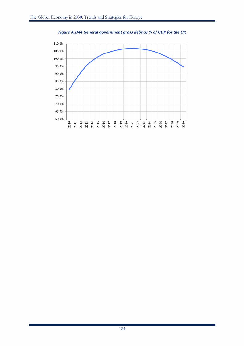
The Global Economy in 2030: Trends and Strategies for Europe
184
Figure A.D44 General government gross debt as % of GDP for the UK
60.0%
65.0%
70.0%
75.0%
80.0%
85.0%
90.0%
95.0%
100.0%
105.0%
110.0%
20
10
20
11
20
12
20
13
20
14
20
15
20
16
20
17
20
18
20
19
20
20
20
21
20
22
20
23
20
24
20
25
20
26
20
27
20
28
20
29
20
30

Annex D. The Results of the NEMESIS Model
185
Appendix 6. The NEMESIS Model
The NEMESIS model (New Econometric Model of Evaluation by Sectoral Interdependency and Supply),
has been partially funded under the fifth, sixth and seventh RTD Framework Programmes of the
European Commission General Directorate of Research.105 NEMESIS is a system of economic models
for every European country, devoted to studying issues that link economic development, competitiveness,
employment and public accounts to economic policies, and notably all structural policies involving long-
term effects: RTD, environment and energy regulation, general fiscal reform, etc. The essential purpose
of the model is to provide a framework for making forecasts, or ‘business as usual’ (BAU) scenarios, of
up to 20 or 40 years, and to assess for the implementation of all additional policies not already involved in
the BAU.
NEMESIS uses among its main data sources EUROSTAT, WIOD and specific databases for external
trade (OECD, CHELEM, New CRONOS), and for technology indicators (OECD and EPO).
The NEMESIS model is recursive dynamic, with annual steps. The main mechanisms of the model are
based on the behaviour of representative agents: enterprises, households, government and rest of the
world. These mechanisms are based on econometric work.
The main originality of the model, when compared to others used for similar policies, lies in the belief
that the medium- and long-term macroeconomic path is the result of strong interdependencies between
sectoral activities that are very heterogeneous from a dynamic point of view.
These interdependencies are exchanges of goods and services on markets, but also of external effects, as
positive technological spillovers. Another originality of NEMESIS is that it is a ‘framework model’ with
different possibilities for the several mechanisms involved in the functioning. Although econometric, the
model cannot be classified as a neo-Keynesian model, as the current version of NEMESIS builds on the
new theories of growth. It also falls outside the classification of a general equilibrium model, as it
incorporates original mechanisms that do not refer to the strict orthodoxy of the mainstream neo-classical
approach on which the general equilibrium approach was based.
Main mechanisms of the model
On the supply side, NEMESIS distinguishes 30 production sectors, including Agriculture, Forestry,
Fisheries, Transportation (4), Energy (6), Intermediate goods (5) Capital goods (5), Final consumption
goods (3), Private (5) and Public services. Each sector is modelled with a representative firm that takes its
production decisions given its addressed demand and input prices. Firms’ behaviour includes innovative
features based on new growth theories, principally endogenous R&D decisions that allow them to
improve their process productivity and product quality. Production in sectors is represented with CES
production functions (with the exception of Agriculture, which uses transcendental logarithmic functions,
and Forestry and Fisheries, where technology is represented with Leontief functions) with five production
factors: capital, unskilled labour, skilled labour, energy and intermediate consumption, where endogenous
innovations of firms can modify the efficiency of the different inputs and the quality of output. The
production function was estimated by the dual approach and estimates and calibration of links between
R&D expenditures, innovations and economic performance were picked up from the abundant literature
on the subject. Interdependencies between sectors and countries are finally captured by a collection of
convert matrices describing the exchanges of intermediary goods, of capital goods and of knowledge in
terms of technological spillovers, and the description of substitutions between consumption goods by a
very detailed consumption module enhancing these interdependencies.
On the demand side, representative households’ aggregate consumption is dependent on current income.
Total earnings are a function of regional disposable income, a measure of wealth for the households,
interest rates and inflation. Variables covering child and old-age dependency rates are also included in an
105 The core teams of the NEMESIS model are: ERASME (France - www.erasme-team.eu) as coordinator, CCIP (France - www.ccip.fr), Federal Planning Bureau (Belgium - www.plan.be), National Technical University of Athens (Greece - www.ntua.gr) and MERIT University of Maastricht.

The Global Economy in 2030: Trends and Strategies for Europe
186
attempt to capture any change in consumption patterns caused by an ageing population. The rate of
unemployment is used, in the short-term equation of consumption (only), as a proxy for the degree of
uncertainty in the economy. Consistent with the other behavioural equations, the disaggregated
consumption module is based on the assumption that there exists a long-run equilibrium, but rigidities are
present that prevent immediate adjustment to that long-term solution. Altogether, the total household
aggregated consumption is indirectly affected by 27 different consumption sub-functions through their
impact on relative prices and total income, to which demographic changes are added. Government public
final consumption and its repartition between Education, Health, Defence and Other Expenditures are
also influenced by demographic changes.
External trade is treated in NEMESIS as taking place through two channels: intra-EU and trade with the
Rest of the World (extra-EU). Data availability was an important factor in this choice – it allowed an
emphasis to be put on intra-EU trade flows, which are a large portion of the total trade in the EU. The
intra-EU and extra-EU export equations can be separated into two components, income and prices. The
income effect is captured by a variable representing economic activity in the rest of the EU for intra-EU
trade, and a variable representing economic activity in the rest of the world for extra-EU trade. Prices are
split into two sources of impacts in each of the two equations (intra-EU and extra-EU trade). For intra-
EU trade, they are the price of exports for the exporting country and the price of exports in other EU
countries. For extra-EU trade, price impacts come through the price of exports for the exporting country,
and a Rest of the World price variable. The stock of innovations in a country (which, in NEMESIS, is
taken relative to the total innovation stock in Europe in a particular sector) is also included in the export
equations in order to capture the role of innovations in trade performance and structural competitiveness.
For imports, equations are identical for both intra-EU and extra-EU trade. The income effect is captured
through domestic sales by domestic producers. The stock of innovations is again included to account for
the effects of innovations on trade performance.
The wage equations, which determine the dynamics of prices and incomes in NEMESIS, are based on a
theory of wage-setting decisions made by utility-maximising unions. The unions calculate utility from
higher levels of employment and from higher real wages (relative to wages outside the sector) in the
sector, subject to the labour demand constraint imposed by firms’ profit maximisation. The implication of
this form of wage equation is that conditions, such as productivity shocks, changes in the unemployment
rate or changes in real wages outside the sector, are important for determining wages and real wages in a
given sector.
Main inputs and outputs of the NEMESIS model
With its original characteristics and great detail-level results, NEMESIS can be used for many purposes
such as short- and medium-term economic and industrial ‘scenarios’, government and local authorities;
analysing business as usual (BAU) scenarios and economy long-term structural change, energy supply and
demand, environment and more generally sustainable development; revealing the long-term challenges of
Europe and identifying issues of central importance for all European, national, and regional structural
policies; assessing for most of Lisbon agenda-related policies and especially knowledge (RTD and human
capital) policies; emphasising the RTD aspect of structural policies that allows new assessments (founded
on endogenous technical change) for policies, and new policy design based on knowledge: education,
skills and human capital and RTD.
NEMESIS has notably been used to study BAU scenarios for the EU and to reveal the implications for
European growth, competitiveness and sustainable development of the Barcelona 3% GDP RTD
objective, of the 7th Research Framework Programme of European Commission, National RTD action
plans of European countries, European policies on greenhouse gas emission reductions, increasing oil
prices, and the European action plan for renewable energies. NEMESIS is currently being used to assess
a European action plan for environmental and energy technologies, a European financial perspective and
the Lisbon agenda, with in-depth development on the modelling of RTD, human capital and labour
markets, and European regions.

187
About the Partners in the Consortium
CENTRE FOR EUROPEAN POLICY STUDIES (CEPS) performs a unique role in the nexus
between academia, business and the public sector as an independent analyst and critic of European policy.
CEPS’ core business is the conduct of policy research on European affairs and the broad dissemination
of findings through a regular flow of publications, public events and electronic commentary. Since its
founding in 1983, CEPS has acquired a solid reputation for integrity and excellence in research and has
amply demonstrated its ability to anticipate trends and analyse policy questions well before they become
topics of general discussion. CEPS’ staff includes 45 in-house researchers and associates organised in
eight units, ensuring a high degree of specialisation and interdisciplinary focus.
Researchers: Daniel Gros, Cinzia Alcidi, Arno Behrens, Steven Blockmans, Matthias Busse, Christian
Egenhofer and Ilaria Maselli
CENTRE D'INFORMATION ET DE RECHERCHE SUR L'ECONOMIE MONDIALE
(CIREM) conducts studies and research on specific demand from private companies, French and
European administrations or international organisations. Some of these projects are conducted in
collaboration with CEPII. CIREM has 20 members (private companies, trade unions, public institutions
and administrations) and is chaired by Francis Ailhaud, Chief Executive Officer of Groupama Asset
Management. The board is mainly composed of representatives from the private sector. CIREM actively
contributes to the rapprochement between the world of research and that of private firms and public
institutions.
Researchers: Lionel Fontagné and Priscila Ramos
ISTITUTO DI STUDI PER L'INTEGRAZIONE DEI SISTEMI (ISIS) is an Italian private
research and consulting firm supporting international, national and local public bodies for the analysis,
design, implementation and evaluation of sustainable policies in the fields of energy, environment,
transport and mobility, urban planning and the knowledge society. ISIS has worked extensively in the
field of policy impact assessment, with particular reference to socio-economic impacts and through the
development and application of forward-looking analysis (FLA) methods and tools. Founded in 1971,
ISIS relies on the expertise of a multi-disciplinary team; including engineers, statisticians, experts in
information technology and economists.
Researchers: Andrea Ricci and Carlo Sessa
SOCIÉTÉ EUROPÉENNE D'ÉCONOMIE (SEURECO) is a company serving the research team
ERASME (Research Team in System Analysis and Economic Modelling) specialised in applied modelling
mainly in the building and use of large scale models for Economy, Energy, Environment and Land Use.
Its staff is composed of nine permanent researchers and three associate researchers. The company
coordinates the development of the economic model NEMESIS (New Econometric Model for
Environment Strategies Implementation for Sustainable Development), and is part of the GEM-E3
model consortium, especially for the modelling of technological change. ERASME’s main activities
consist of building applied models (general and partial equilibrium, calibrated or econometric) and then
using them to assess for European and National public policies for RTD, Energy, Environment, Land-
Use, Financial Reforms, Taxation, etc.
Researchers: Paul Zagame, Arnaud Fougeyrollas and Gilles Koléda.